the Creative Commons Attribution 4.0 License.
the Creative Commons Attribution 4.0 License.
 | 30 Nov 2022
A 1 km daily soil moisture dataset over China using in situ measurement and machine learning
Qingliang Li
Gaosong Shi
Vahid Nourani
Jianduo Li
Lu Li
Feini Huang
Ye Zhang
Chunyan Wang
Dagang Wang
Jianxiu Qiu
Xingjie Lu
Yongjiu Dai
High-quality gridded soil moisture products are essential for many Earth system science applications, while the recent reanalysis and remote sensing soil moisture data are often available at coarse resolution and remote sensing data are only for the surface soil. Here, we present a 1 km resolution long-term dataset of soil moisture derived through machine learning trained by the in situ measurements of 1789 stations over China, named SMCI1.0 (Soil Moisture of China by in situ data, version 1.0). Random forest is used as a robust machine learning approach to predict soil moisture using ERA5-Land time series, leaf area index, land cover type, topography and soil properties as predictors. SMCI1.0 provides 10-layer soil moisture with 10 cm intervals up to 100 cm deep at daily resolution over the period 2000–2020. Using in situ soil moisture as the benchmark, two independent experiments were conducted to evaluate the estimation accuracy of SMCI1.0: year-to-year (ubRMSE ranges from 0.041 to 0.052 and R ranges from 0.883 to 0.919) and station-to-station experiments (ubRMSE ranges from 0.045 to 0.051 and R ranges from 0.866 to 0.893). SMCI1.0 generally has advantages over other gridded soil moisture products, including ERA5-Land, SMAP-L4, and SoMo.ml. However, the high errors of soil moisture are often located in the North China Monsoon Region. Overall, the highly accurate estimations of both the year-to-year and station-to-station experiments ensure the applicability of SMCI1.0 to study the spatial–temporal patterns. As SMCI1.0 is based on in situ data, it can be a useful complement to existing model-based and satellite-based soil moisture datasets for various hydrological, meteorological, and ecological analyses and models. The DOI link for the dataset is http://dx.doi.org/10.11888/Terre.tpdc.272415 (Shangguan et al., 2022).
- Article
(11497 KB) - Full-text XML
-
Supplement
(5321 KB) - BibTeX
- EndNote


Soil moisture (SM) plays a key role in land–atmosphere interactions through its strong impacts on the water and carbon cycle (Entekhabi et al., 1996; Seneviratne et al., 2010; Wagner et al., 2007). The status of SM is closely related to climate and weather conditions (Dirmeyer et al., 2006). The high-quality SM data with a fine spatial–temporal scale can be valued as indispensable tools for observing the extreme weather events, e.g., droughts (e.g., Chawla et al., 2020; Mishra et al., 2017; Tijdeman and Menzel, 2021), floods (e.g., Kim et al., 2019; Norbiato et al., 2008; Parinussa et al., 2016), and carbon cycle modeling (O and Orth, 2021). Further, SM is also identified as an important component of the Essential Climate Variables by the Global Observing System for Climate (GCOS, 2016). However, high-quality SM data acquisition is a challenging task due to the complicated spatiotemporal variations of the SM (Guo and Lin, 2018; Ojha et al., 2014; Vereecken et al., 2014). Such spatiotemporal variations of SM are usually affected by the inherent heterogeneity of soils, land cover, and weather (Brocca et al., 2007; Crow et al., 2012; Vereecken et al., 2014).
At present, the methods for SM data estimation can be divided into five categories: in situ observations, satellite observations, offline land surface model simulations, Earth system model simulations, and reanalysis products. For in situ SM observations, SM data are usually measured by the probe measurement method (Orth and Seneviratne, 2014), in which as direct observations this method usually leads to lower errors than satellite observations, land surface model simulations, Earth system model simulations, and reanalysis products (Pan et al., 2019). Although a large number of stations are distributed all over the world, there are still many regions with no in situ SM observations due to financial constraints (Karthikeyan and Kumar, 2016), and field stations are too sparse to capture adequate spatial coverage (Gruber et al., 2016). For satellite observations, SM data are mainly retrieved by microwave radiometers (frequencies are less than 12 GHz) on satellites (Entekhabi et al., 2010; Fujii et al., 2009; Kerr et al., 2010), which can provide the global SM data with uniform distributions, but for the microwave-radiometer-measured SM data from the near surface, only the top-layer SM (typically ∼ 5 cm) can be retrieved and the data gaps exist in regions with dense vegetation and snow-covered or frozen soils. The SM data of the offline land surface model and Earth system model simulations span multiple soil layers and have a seamless spatial distribution (Gu et al., 2019), but they both have uncertain and different forcing factors due to the spatial sub-grid heterogeneity of soil properties and vegetation, thus leading to large differences from in situ SM observations (Dirmeyer et al., 2006; Kumar et al., 2009). Reanalysis products can also provide SM data with good temporal variations by assimilating observations into land surface models or Earth system models (Chen et al., 2021). They can also provide SM data at deeper soil depth than satellite observations, but reanalysis products usually lead to higher disagreement with in situ SM observations when the assimilated meteorological variables (e.g., precipitation) are biased (Balsamo et al., 2015).
In brief, the characteristic strong points and shortcomings both coexist in each type of SM product. Hence, we are eager to develop the high-quality SM product which comprehensively has a high-resolution seamless spatial distribution, long time periods, and low errors from the above SM products.
Recently, machine learning (ML) models have been successfully applied for predicting (Li et al., 2021; Mohamed et al., 2021; Xu et al., 2010) or downscaling (Chakrabarti et al., 2014; Srivastava et al., 2013; Wei et al., 2019; Mao et al., 2022) the SM values. They capture the complex nonlinear relationship between SM and all available predictors related to SM variation (e.g., meteorological variables, land cover, and soil data) with better accuracy. ML models provide the capacity to estimate high-quality SM data based on in situ SM measurements (Sungmin and Orth, 2020) and further to improve the generated SM product with low errors and seamless spatial distribution for long time periods. Random forest (RF) methods such as the ML method were applied by Zeng et al. (2019) to generate 0.5 km daily SM data for the period from 2010 to 2014 over Oklahoma based on in situ SM records and satellite observations. The low root mean square error (ranging from 0.038 to 0.050 m3 m−3 for the year-to-year test and from 0.044 to 0.057 for the station-to-station test) was obtained from experiments, demonstrating the accuracy of the gridded SM data. O and Orth (2021) used the long short-term memory (LSTM) model as a deep learning approach to estimate daily SM data over the whole world at 27.75 km spatial resolution for the period from 2000 to 2019, stating the superiority of their SM data over the ERA5 dataset. It was necessary to note that the above two studies both emphasized that the applied in situ SM observations could not cover all the tested regions, leading to relatively high uncertainty outside the training conditions. In other words, the more in situ SM stations in the test region, the higher the quality of gridded SM data by ML models. Additionally, Carranza et al. (2021) used the RF model to estimate root zone SM within a small catchment from 2016 to 2018 and demonstrated that the ML model had slightly higher accuracy than a process-based model combined with data assimilation for data-poor regions. Karthikeyan and Mishra (2021) applied extreme gradient boosting (XGBoost) to estimate daily SM data over the United States, with about 1 km resolution for the period from 31 March 2015 to 29 February 2019 (only 1431 d), and the results showed that the estimations can capture temporal variations of SM well.
China is one of the largest countries in the world, reaching from central to eastern Asia. The climate types are complex and diverse and span the wet, semi-humid, semi-dry, and dry climate types from southeast to northwest, and the northward extent and intensity of summer monsoon often cause significant changes in precipitation and arid–humid climate (Cong et al., 2013). Since SM and precipitation can interact with each other (Li et al., 2020), in situ data-based estimation of SM is a challenging task due to such heterogeneity and complex spatiotemporal variabilities.
Previous studies have already provided several gridded SM products covering China or the world but mainly based on remote sensing data and only for the surface layer (e.g., Chen et al., 2021; Meng et al., 2021; Wang et al., 2021 and Q. Zhang et al., 2021). However, there is still a big gap in the technical literature about daily SM data with high quality (high-resolution seamless spatial distribution, long time periods, and low errors) at multiple layers based on in situ measurements for China. Although O and Orth (2021) generated the global SM data with the ML model which includes the China region, only data from about 20 in situ SM stations have been applied for SM modeling for the whole of China. In addition, the resolution of this product is 0.25∘, which limits its use in regional applications when high-resolution SM is required.
To fill this research gap, in this study, we aimed at generating high-quality gridded SM data over China using in situ measurements and the RF model (Fig. 1). The predictors consisted of static data and time series variables, including ERA5-Land (the land component of the fifth generation of European Reanalysis, Muñoz Sabater, 2019, 2021), the USGS (United States Geological Survey) land cover type (Loveland et al., 2000), the USGS DEM (digital elevation model, Balenović et al., 2016), the reprocessed MODIS LAI (MODerate-resolution Imaging Spectroradiometer Leaf Area Index, Yuan et al., 2011), and the CSDL (China Soil Dataset for Land surface modeling, Shangguan et al., 2013). The in situ SM observations from 1648 stations were employed as the SM modeling target after quality control procedures.
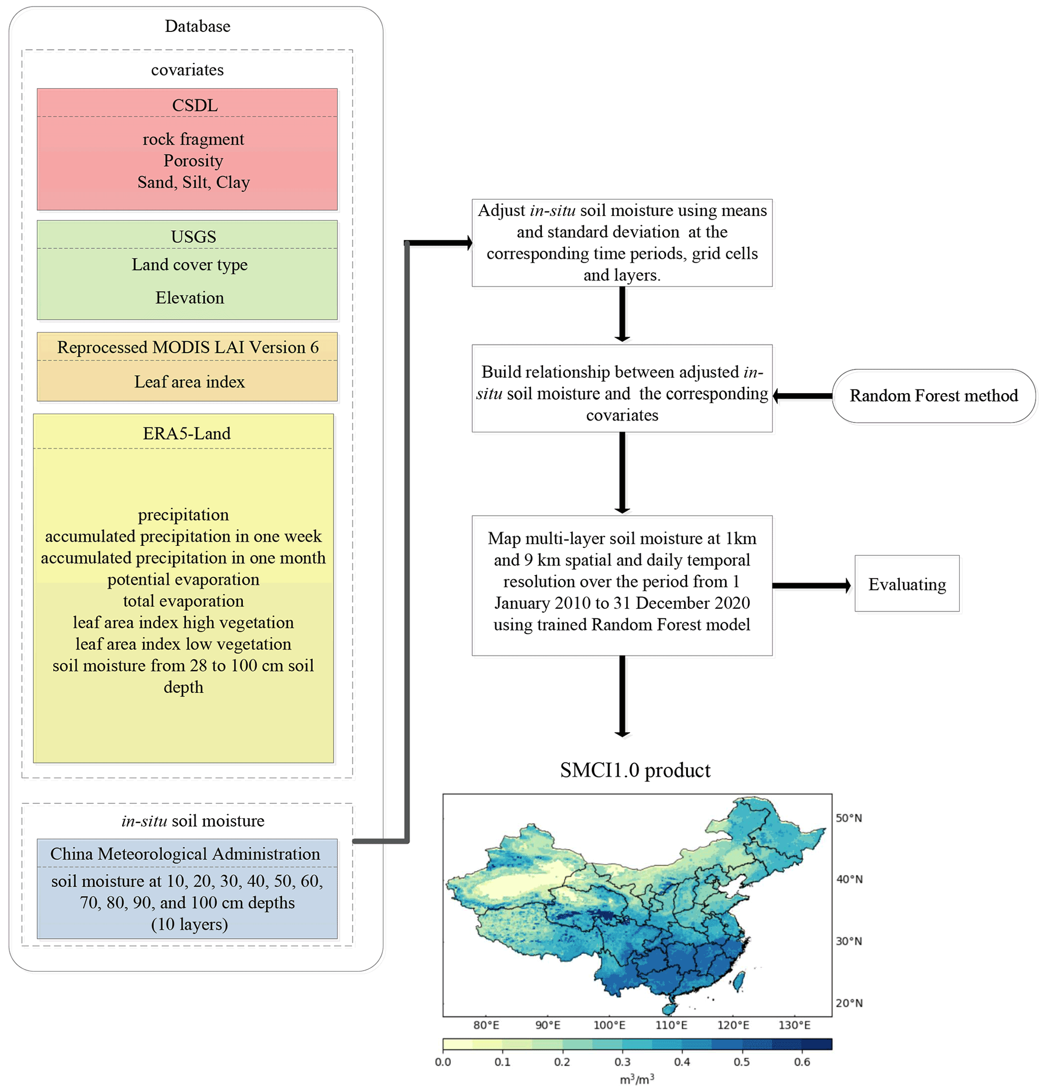
Figure 1Generation process for the SMCI1.0 product with 1 km spatial resolution and daily temporal resolution over the period from 1 January 2000 to 31 December 2020 over China.
The new Chinese gridded SM product (SMCI1.0, Soil Moisture of China by in situ data, version 1.0) provides SM data at 10 layers, which include soil depths from 10 to 100 cm with an interval of 10 cm. Meanwhile, SMCI1.0 has ∼ 1 km (30 s) spatial resolution and daily temporal resolution over the period from 1 January 2010 to 31 December 2020. For the SMCI1.0 product, we mainly considered answering the following research questions.
-
What is the sensitivity of the in situ SM data to all the predictors, including meteorological data (air temperature, precipitation, total evaporation, potential evaporation), soil data (SM and soil temperature at different soil layers, static soil properties), leaf area index, and land cover type.
-
Can the RF model successfully generate high-quality gridded SM (high-resolution seamless spatial distribution, long time periods, and low errors) at multiple layers over China based on in situ SM observations?
-
How does the RF model perform for spatiotemporal estimation of SM in the year-to-year and station-to-station scenarios?
-
What are the conditions under which SMCI1.0 SM data may lead to lower errors and higher errors against adjusted in situ SM observations?
For the above issues, we make four contributions to generating and validating multi-layer gridded SM data over China. First, we record and make a detailed analysis of the correlations between in situ SM and all predictors. Then, we apply the RF to model the complex relationship between predictors and in situ SM observations and further validate it using year-to-year and station-to-station experiments. Finally, we intuitively display and analyze the quality of SMCI1.0 under different conditions, which can help the researchers to improve the Chinese gridded SM intentionally and strategically. Section 2 describes the in situ SM data, the predicting data, the RF model, and its application in SM estimation. Section 3 gives the validation results, experimental results, a sampled map on a day, and the relative importance of the predictors. Sections 4 and 6 present the discussion and conclusions, respectively.
2.1 In situ SM observations
Target SM data for the RF model were constructed from the CMA SM observations. The dataset contains hourly data from 1789 stations over China for 1 January 2010 to 31 December 2020. The spatial distribution of the observations is shown in Fig. S1a. It should be noted that data from such a large number of in situ stations can help ML models to capture the complex nonlinear relationship between SM and predictors under various training conditions and thus to generate high-quality gridded SM data. The automated quality control of in situ SM observations was performed before training the RF model. We first removed the null values over the long period (10 d time step) and outlier/unreasonable SM values. To check the unreasonable SM values, four plausibility checks were performed, such as checking geophysical consistency using precipitation and soil temperature, spike detection, break detection, and constant value detection. The details can be found in the Global Automated Quality Control method (Dorigo et al., 2013). Finally, the removed values were replaced by the linear interpolation method according to the remaining SM values in the same time period from 5 d ahead to 5 d later. To facilitate the generation of 1 km gridded SM data at multiple layers by the RF model, the CMA SM observations were processed to daily ones, and the observations were averaged if there was more than one station within a grid at 1 km resolution. We simply averaged all the available observations on each day and all stations if there was more than one station within each grid with 1 km resolution. In this way, we got 1648 spatial points (or grids) of observations. The description of in situ SM can be found in the Supplement (Sect. S1 and Fig. S1).
After the above data processing, the correction of the deviation and variance of the in situ SM was performed, which can help the ML model to achieve the high-quality SM product. In situ SM data have been obtained by various sensor types with different calibration processes. Hence, to overcome the artifacts during the RF model training, we adjusted the observations to match the means and standard deviations of the ERA5-Land SM in the corresponding time periods, grid cells, and layers using the method proposed by Sungmin and Orth (2020). In this method, we first obtained a weight by dividing the standard deviations of the in situ SM at each station by that of the ERA5-Land SM at the corresponding grid, and then we multiplied the original in situ SM by this weight. After that, we computed the difference between the average value of the in situ SM at each station and the ERA5-Land SM at the corresponding grid and subtracted the in situ SM from the computed difference. This method made the target in situ SM resemble the mean and standard deviation of the ERA5-Land SM and retained daily temporal variations which follow the original in situ SM time series. As the soil depth of each soil layer of the ERA5-Land SM was inconsistent with that of the in situ SM, we mapped the soil layer of the ERA5-Land SM to the corresponding soil layers of the in situ SM. Hence, the in situ SM data from 10 to 30 cm were adjusted based on the gridded SM at layer2 from the ERA5-Land dataset (7–28 cm), and the in situ SM data from 30 to 100 cm were adjusted based on the gridded SM at layer3 from the ERA5-Land dataset (28–100 cm).
2.2 Datasets as predictors
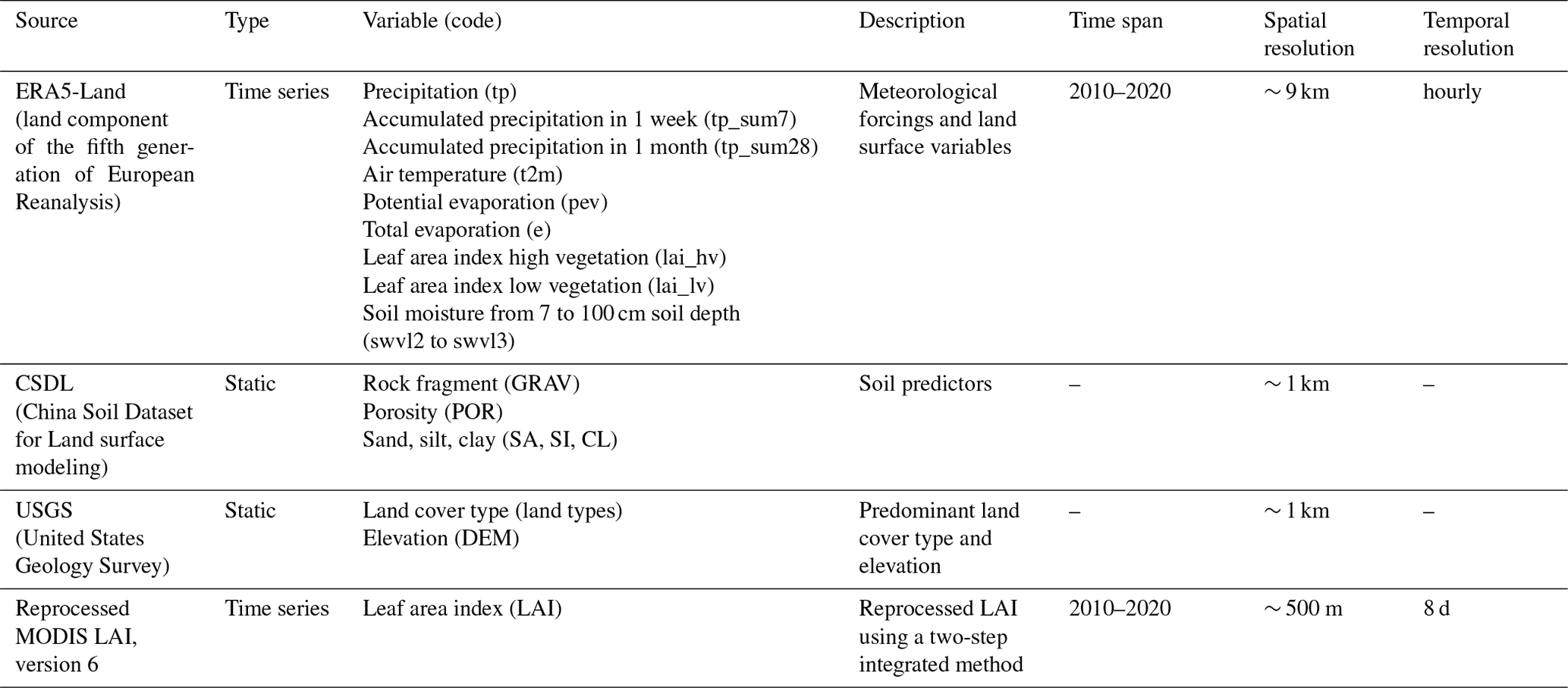
Table 1 shows the used predictors for the RF model. Most predictors were collected from the ERA5-Land reanalysis dataset, which is an enhanced version of the ERA5 land component forced by meteorological fields from ERA5. The reasons for selecting the ERA5-Land dataset as a preference were as follows. (1) It is generated under a single simulation of a land surface model using ERA5 reanalysis as the forcing data but with a series of improvements which make it more accurate for all types of land applications (Muñoz-Sabater et al., 2021). (2) ERA5-Land is currently updated with 2–3 months' latency, which allows us to update SMCI1.0 in time. (3) ERA5-Land is long-term (since 1950) data and has a seamless spatial distribution and multiple layers, which makes it possible to generate high-quality SMCI1.0. Compared with satellite observations, we can avoid the spatial–temporal gaps and limited time periods covered by using ERA5-Land reanalysis (Sungmin and Orth, 2020). The static data of predictors were collected from the USGS land cover type (Loveland et al., 2000) and the DEM (Balenović et al., 2016), the reprocessed MODIS LAI Version 6 for land surface and climate modeling (Yuan et al., 2011), and the CSDL (Shangguan et al., 2013), including sand, silt, and clay content, rock fragments, and bulk densities. The reprocessed MODIS LAI Version 6 was improved by a two-step integrated method with continuity and consistency in the space and time domains (Yuan et al., 2011). It was worth noting that the temporal resolution of the reprocessed MODIS LAI Version 6 was 8 d, and the daily LAI between the 8 d was computed by linear interpolation of the nearest two LAI values at a 8 d time step. CSDL was derived by the polygon linkage method, whose results are consistent with common knowledge of Chinese soil scientists (Shangguan et al., 2013). All the predictors were processed to the same 1 km by 1 km grid system. ERA5-Land data with 9 km resolution were resampled into 1 km by the nearest neighbor method, and the MODIS LAI with 500 m resolution was aggregated into 1 km by averaging.
Table 1Details of the predictors for training the random forest model.
2.3 RF
RF is an ensemble machine learning approach that applies the decision tree and bagging methods for the classification and regression problem (Breiman, 2001). The simple decision tree model partitions the variable space and further groups the datasets recursively based on similar instances. For the candidate variables from a set of predictors, a split is determined by the values of the desired variable that evolves into a tree structure with multiple parent and child nodes. Meanwhile, the response variance for decision regression trees is applied as the criterion to maximize the purity of each node (the response variance is applied to measure node purity) and further to find the optimal split. RF generates diverse decision trees to avoid overfitting through the bagging method, which constructs multiple training sub-datasets by resampling with replacement of the original dataset. For each training sub-dataset, a decision tree grows until the pre-assumed criterion is reached (e.g., the value for the minimum node size). When all decision trees are generated, the average of all the estimations from each decision tree is computed.
The importance of the predictors obtained by the RF model is also worth noting and can be explored with a permutation method. In the permutation method, different SM values are estimated by permuting all the predictors. Hence, the importance of the predictors can be detected by comparing the accuracy of the SM estimation. For example, if one predictor is dominant in estimating the target SM, the estimated SM value accuracy is expected to be lower using the other non-permuted predictors.
2.4 The application of the random forest model
In this study, we first determined the optimal values of hyper-parameters in the RF model based on the 10-fold cross-validation method. After calibration of the hyper-parameters, two independent experiments were conducted to investigate the estimation accuracy of the developed SMCI1.0 spatial–temporal data (year-to-year and station-to-station experiments). In the year-to-year experiments, the data from 2010 to 2017 at each station were reserved for the training set, and to evaluate the accuracy of SMCI1.0 at the temporal scale, we compared the SM generated by the RF model with the in situ SM data from 2018 to 2020. In the station-to-station experiments, the randomly selected data from two-thirds of the stations from 2010 to 2020 were applied for training, and the data of the remaining stations were used to evaluate the accuracy of SMCI1.0 at the spatial scale. Finally, the SMCI1.0 product was generated by the RF model at 1 km resolution based on the in situ SM and predictors (shown in Table 1) from all stations and all years. In addition to the 1 km resolution, we also produced a version of 9 km resolution by aggregating the higher-resolution predictors for the convenience of applications when coarser SM data are needed in broad-scale studies. In addition to the period of 2010–2020 when in situ SM data are available, we also produced the gridded SM for the period of 2000–2009 when in situ SM data are unavailable, assuming that the relationship between SM and the predictors remained the same in the last 2 decades. It is proper to suppose that the data quality during 2000–2009 is poorer than that of 2010–2020.
The number of randomly selected variables from all the predictors (max_features) and the value for the minimum node size (min_samples_leaf) are the vital hyper-parameters for the RF model, which can affect the modeling performance. Other hyper-parameters, such as the number of trees (n_estimators), were not determined based on the RF's own training. Meanwhile, to prevent an overfitting problem, we applied the 10-fold cross-validation method to tune the values of max_features and min_samples_leaf in the range [1,25] with a single interval and [5,30] with five intervals via the gridded direct search method. The accuracy of RF models with all hyper-parameters calibrated by the direct search method at 10 cm soil depth is shown in Table S1. It can be seen that the root mean square error (RMSE) obtained based on all the hyper-parameters ranged from 0.601 to 0.637, and the best accuracy (RMSE = 0.601) could be achieved when max_features and min_samples_leaf were set to 1 and 20, respectively, and they are used for the remaining modeling of this study.
The modeling performance and quality of the SMCI1.0 product were evaluated in terms of ubRMSE, MAE (mean absolute error), R (correlation coefficient), R2 (explained variation), and bias, respectively. ubRMSE and MAE were applied to test the ability to estimate volatility and fluctuation amplitude, respectively. R denotes the fluctuation pattern and R2 represents the percentage of variance explained by the RF model. Bias was used to observe whether the estimations were overestimated or underestimated. These metrics were computed as follows:
where yi and xi denoted the ith in situ SM and gridded SM for all the stations and periods, respectively. and represented the mean values of the in situ SM and gridded SM, respectively.
3.1 Validation of RF-based SM modeling
To evaluate and validate the performance of the RF model in generating SMCI1.0, we mainly discussed the modeling ability with year-to-year and station-to-station experiments, which could ensure that the SMCI1.0 product has low errors on both temporal and spatial scales against in situ SM records. Meanwhile, we also compared the results with the state-of-the-art global gridded datasets such as ERA5-Land, SMAP-L4, and SoMo.ml.
The scatter plot of the mean values of SMCI1.0 and in situ SM data for each station, the frequency distributions of all SM values in SMCI1.0 and in in situ measurements, and the violin plot for the distribution of daily SM from stations for each climate type are presented for the year-to-year experiment in Fig. 2 (from 10 to 30 cm soil depths) and Fig. S2 (from 40 to 100 cm soil depths). As shown in Fig. 2a, we can conclude that there is generally good agreement between the mean of SMCI1.0 and that of in situ SM at each station (the correlation ranges from 0.867 to 0.908), which demonstrates that the RF model can capture spatial variations in in situ SM well. The RF model showed somewhat better results at deeper soil depths, such as the RF model at 30 cm soil depth, which had a better performance than that at 10 and 20 cm soil depths as shown by Fig. 2a, which was consistent with the previous studies (e.g., Sungmin and Orth, 2020). The worst results were achieved by the RF model at 70 and 90 cm soil depths, as shown by Fig. S2a (ubRMSE = 0.053, MAE = 0.038, R=0.867, R2=0.731 at 70 cm soil depth; ubRMSE = 0.052, MAE = 0.036, R=0.883, R2=0.759 at 90 cm soil depth). Meanwhile, the best result was achieved by the RF model at 30 cm soil depth (ubRMSE = 0.043, MAE = 0.033, R=0.908, R2=0.824). As shown by Fig. 2b, although SMCI1.0 yielded less variability in the value ranges from 0 to 0.18, 0.38 to 0.43, and 0.46 to 0.6 and higher variability in other ranges, as a whole, SMCI1.0 data generally agree well with in situ SM values. The same conclusion can be drawn from the 40 to 100 cm soil depths in Fig. S2b. The SMCI1.0 data were further evaluated for each climate type in Figs. 2c and S2c. With regard to the violin plot, the RF model could estimate consistent results with in situ SM. However, the inconsistent SM was estimated in a tropical monsoon climate (Am) and desert climate (Bw). The reason could be attributed to only a few in situ SM data in these climatic regions, as presented in Fig. S1e. Finally, we concluded that the RF model can reproduce the temporal variation in in situ SM data accurately in an unseen period.
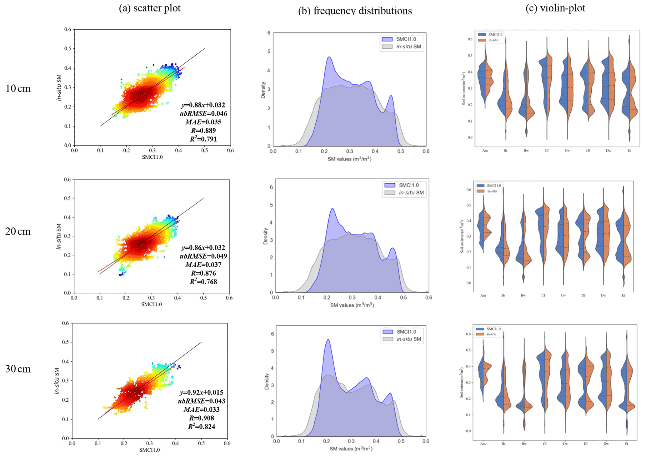
Figure 2Comparisons between SMCI1.0 and in situ SM from 10 to 30 cm soil depth in the year-to-year experiment: comparison of (a) the scatter plot between the mean of SMCI1.0 and that of in situ SM at each station, (b) the frequency distributions of all SM values in SMCI1.0 and that in in situ measurements, and (c) the violin plot for the distribution of daily SM from stations for each climate type.
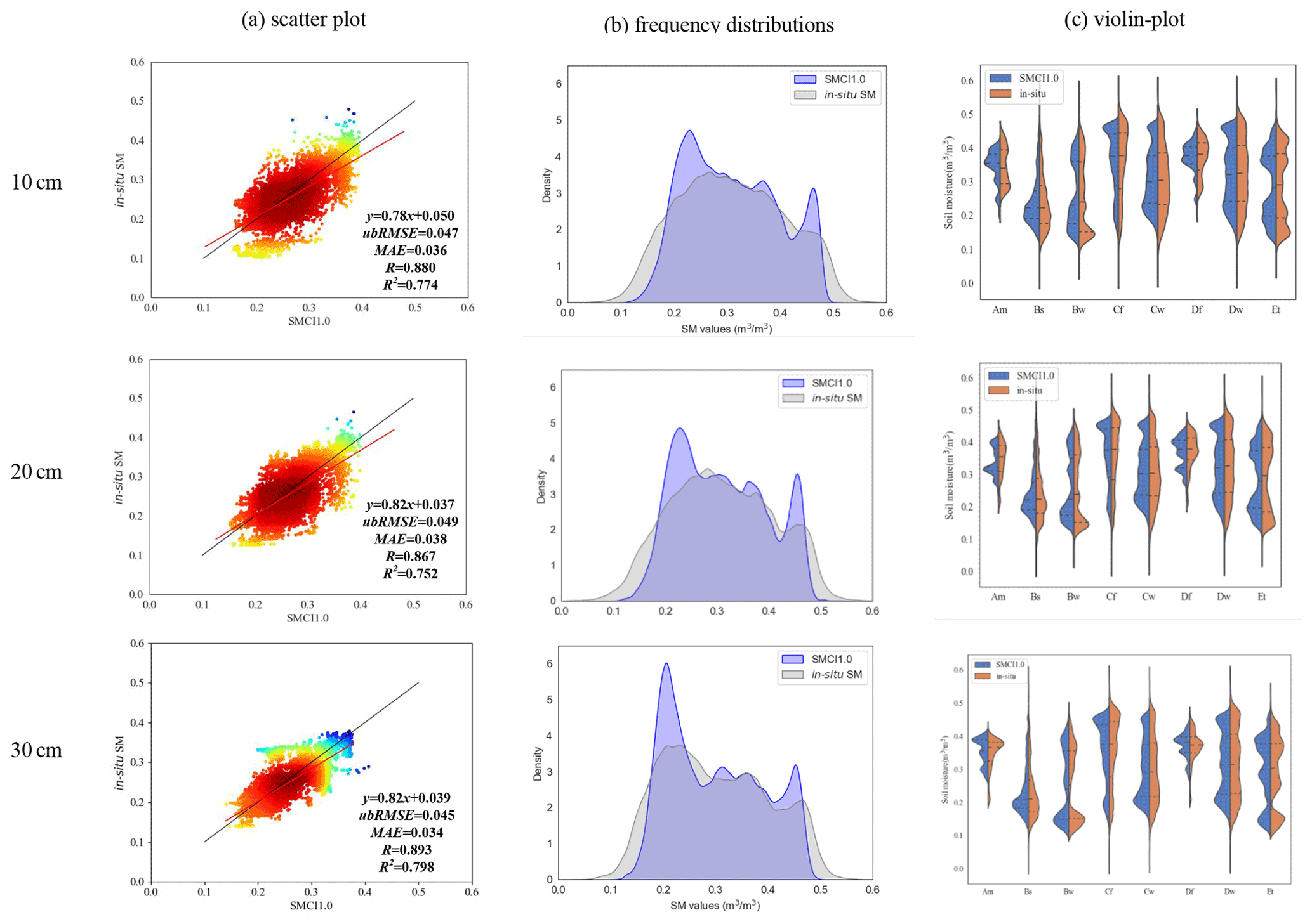
It is clear from Figs. 3 and S3 that, although the results of the station-to-station experiment were inferior to those of the year-to-year estimation, the RF model could also perform well in estimating seamless SM over China at unseen locations. Additionally, similarly to the year-to-year experiment, the RF model performed better at 30 cm soil depth than those at other soil depths in the station-to-station experiment.
Finally, we compared the SMCI1.0 product with other gridded datasets (ERA5-Land, SoMo.ml, and SMAP-L4) according to the median ubRMSE, R, bias, and MAE. According to Figs. 4 and S4, the SMCI1.0 product provides the lowest median ubRMSE and MAE values for the 10 to 100 cm soil depths. Considering the median bias between gridded SM and in situ SM observations, the SMCI1.0 product shows an almost similar accuracy to ERA5-Land datasets for all depths but a higher accuracy than the SoMo.ml and SMAP-L4 datasets. It was worth noting that the SMAP-L4 dataset has the widest spread of errors and tended to underestimate in situ measurements, which led to higher median ubRMSE and MAE values. Regarding the median R between gridded SM and in situ SM observations, the SMCI1.0 product has a slightly higher quality than the SoMo.ml dataset for 10, 20, 80, and 100 cm soil depths and obvious advantages over the ERA5-Land and SMAP-L4 datasets for all depths, while it had a lower quality than the SoMo.ml dataset for the other soil depths. Considering all the above metrics, the SMCI1.0 product provides more robust data than some other commonly used gridded datasets.

Figure 4Comparison between gridded datasets (SMCI1.0, ERA5-Land, SoMo.ml, and SMAP_L4) at soil depths of (a) 10 cm, (b) 20 cm, (c) 30 cm, and (d) 40 cm. The red lines indicate the zero value for bias and the best performance among datasets for ubRMSE, R, and MAE.
Overall, the RF model could be able to successfully generate the SM data with low errors, taking in situ SM observations as the reference in unseen periods and locations. According to the comparison analysis, the SMCI1.0 product outperforms some other SM products, including ERA5-Land, SoMo.ml, and SMAP-L4.
3.2 The spatial and temporal evaluation of SMCI1.0
Overall performance of the proposed modeling and accuracy of the SMCI1.0 dataset were evaluated in Sect. 3.1, but nothing was presented there about the variability and trend of this dataset at different temporal and spatial scales. Hence, to evaluate the temporal variation of the SMCI1.0 data, we randomly selected stations from different climate regions to evaluate the dynamics of the SM data in SMCI1.0, ERA5-Land, SMAP-L4, SoMo.ml, and in situ SM from 10 to 20 cm soil depths. On the other hand, for the spatial scale, we represented the estimation performance for each in situ SM station in terms of ubRMSE, R, and bias. Notably, a year-to-year experiment was conducted to evaluate each station as much as possible.
Figure 5 compares the temporal dynamics of the SM data from SMCI1.0, ERA5-Land, SMAP-L4, SoMo.ml, and in situ datasets at 10 cm soil depth along with local precipitation. We could see that, although the SMCI1.0 product shows a large deviation compared with the in situ SM in the snow climate and fully humid zone (Df-51431: E, N), it was almost consistent with in situ SM in other regions. It is necessary to note that the SM values in the desert climate region (Bw-W1063: E, N) show higher variability but low precipitation from the 231st to 325th days, and the SMCI1.0 product could still adequately capture their relationship (represented in the light blue rectangle). Overall, and similarly to in situ data, SMCI1.0 data reasonably follow the consistency with climate conditions as SM is increased and decreased under wet and dry conditions, respectively.
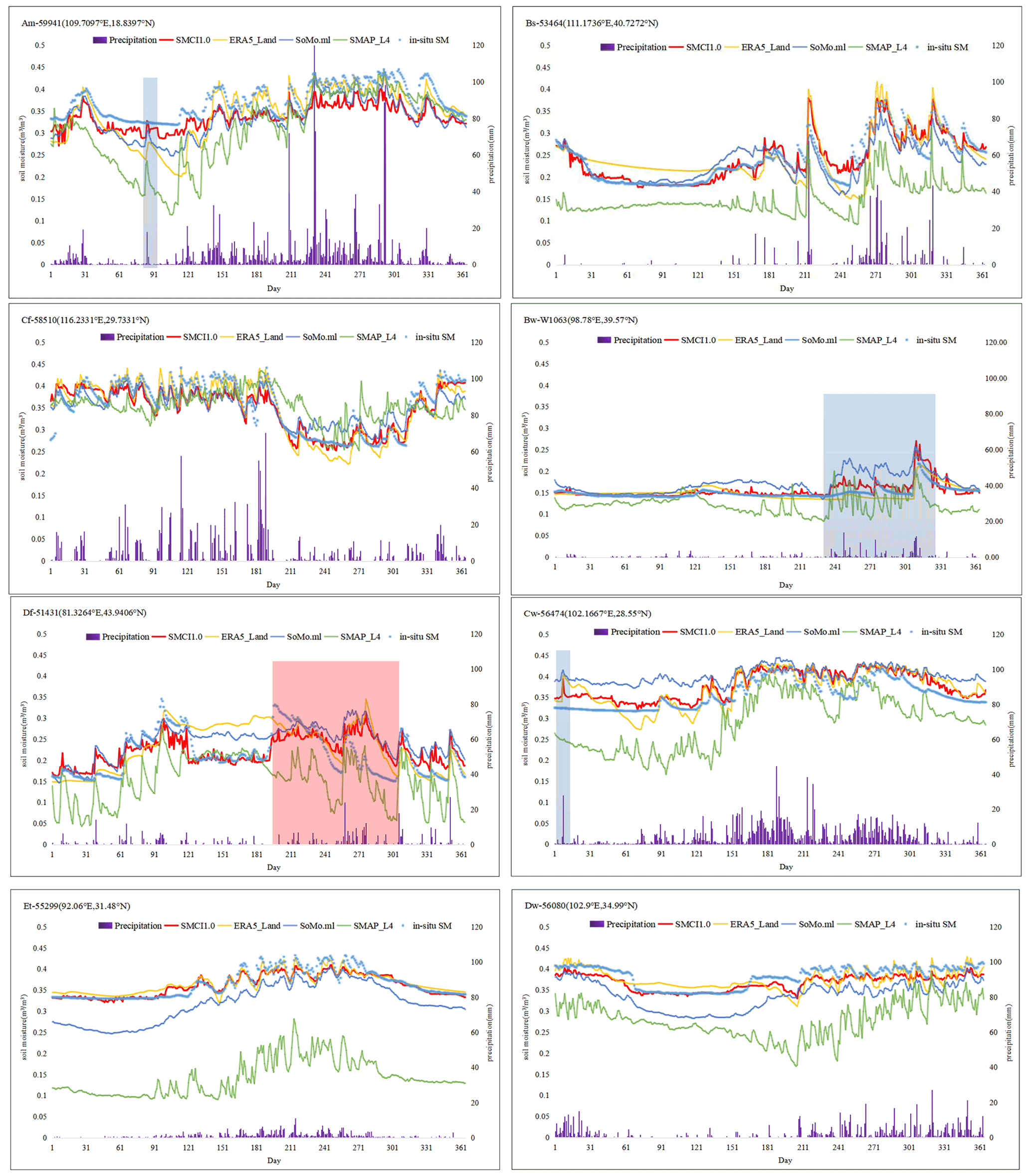
Figure 5Time series of in situ and estimated SM by the RF model at 10 cm soil depth along with daily precipitation in different climatic zones.
Figure 6 represents the in situ testing performance according to the ubRMSE, R, bias, and MAE values. We could see that the SMCI1.0 product led to relatively low ubRMSE, bias, and MAE over most regions. Additionally, Fig. 7 shows that the low errors of the SMCI1.0 product often appeared in the arid regions, which was consistent with the previous study (Zhang et al., 2019). However, the higher ubRMSE and MAE and lower R values could be seen in the North China Monsoon Region. The North China Monsoon Region has typical temperate monsoon climate characteristics, where the annual temperature is high and the rainy season is concentrated. The SM variations in the North China Monsoon Region were complex, which may present great challenges for estimating SM with the RF model. Except for the North China Monsoon Region, SMCI1.0 data mostly led to R values larger than 0.5. According to the bias in Fig. 6, we could see that the SMCI1.0 product tends to be underestimated in northeastern and southwestern China and overestimated in eastern China, which had a similar trend to the ERA5-Land dataset, which can also be confirmed by the box plot of bias in Fig. 5. The SMCI1.0 product led to lower errors than SoMo.ml in estimating in situ SM. Meanwhile, the SMCI1.0 product is often underestimated in northern China but overestimated in Sichuan Province (97∘21′ E–108∘12′ E, 26∘03′ N–34∘19′ N), in contrast to the SoMo.ml dataset. According to the R values in Fig. 6, the SMCI1.0 product led to similar results to the SoMo.ml dataset and performed better than the ERA5-Land and SMAP-L4 datasets, which could also be represented by the box plot of R in Fig. 5.

Figure 6Goodness-of-fit statistics (ubRMSE, R, bias, and MAE) at 10 cm soil depth for the RF model during the tested period.
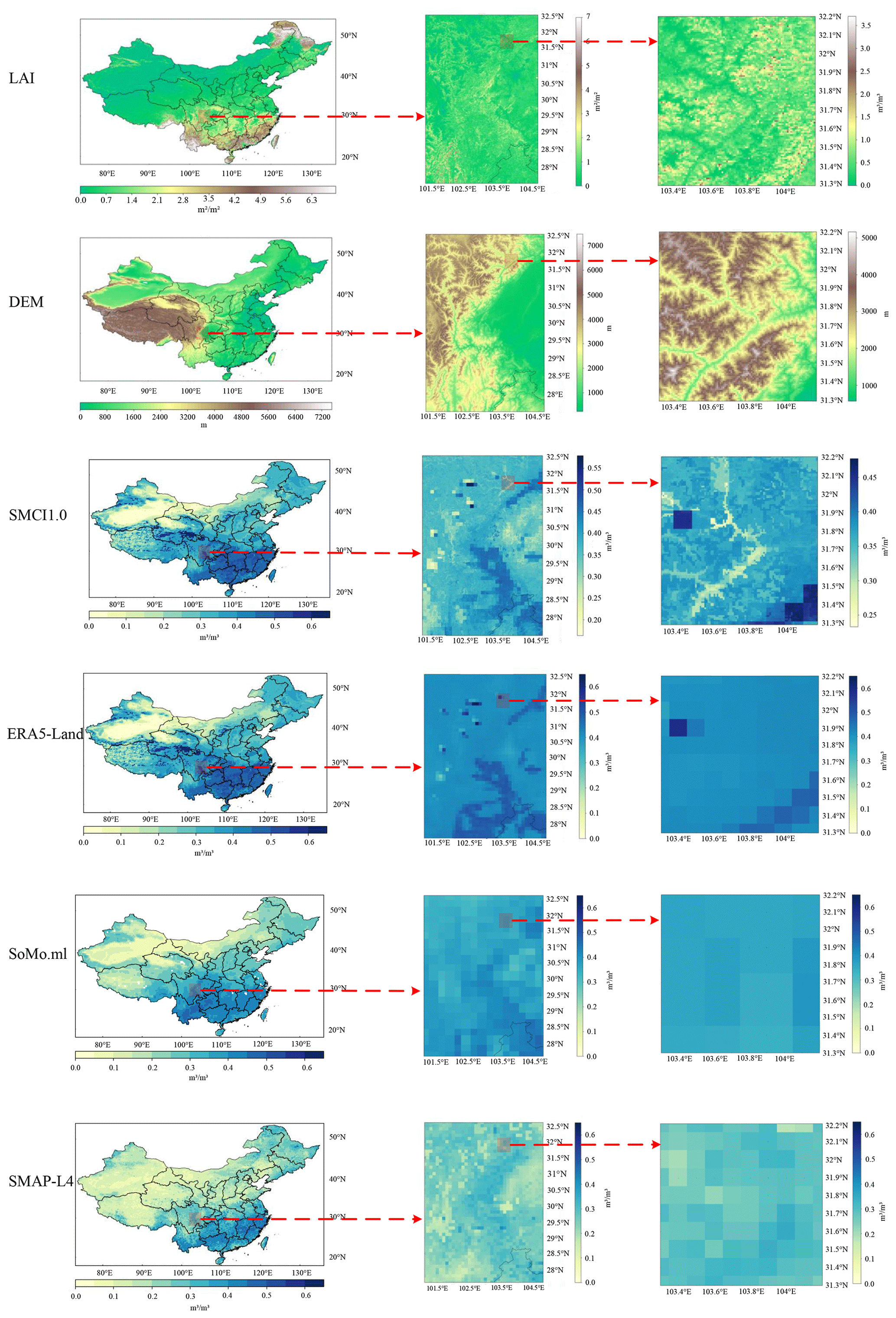
Figure 7Soil moisture maps from different products on 1 January 2016. The resolution is 1 km for SMC1.0, 9 km for ERA5-Land and SMAP-L4, and 0.25∘ for SoMo.ml.
3.3 Spatial patterns of SMCI1.0
To describe the general spatial patterns of SMCI1.0 over China, as an example, the 1 km SM maps are presented for 1 January 2016 by Fig. 7, which shows that the spatial contiguity of SM patterns for SMCI1.0 could be captured well, and most high-resolution details of SM patterns in all the climatic regions for SMCI1.0 had a more detailed “expression” than that for the other SM products. Meanwhile, the spatial pattern of SMCI1.0 was more consistent with those of high-resolution predictors such as the DEM and LAI in some regions, which indicated that SMCI1.0 could better reflect the detailed spatial distribution of SM. Southeastern China is the tropical monsoon climate zone, where the rainy season was concentrated (presented in Fig. 5). Hence, these regions are predominantly wet in the SM maps. Northwestern China is the desert climate region, with few rainfall and dry conditions (also represented in Fig. 5). Qinghai Province (89∘35′ E–103∘04′ E, 31∘09′ N–39∘19′ N) belongs to the tundra climate zone, where some soils are wet and others are dry. This is probably due to the complicated topography of Qinghai Province in that some regions with woody plants can intercept rainfall, which may decrease the overall water input into the soil (Zwieback et al., 2019), and other regions with vegetation can decrease soil temperature and evaporation from the soil surface by shading, preventing the loss of soil moisture (Kemppinen et al., 2021).
4.1 Relative importance of predictors
The relative importance of predictors at the 10 soil depths is shown in Figs. 8 and S7. Bars present the variability of the relative importance across the predictors. As presented in Fig. 8, the ERA5-Land SM is the most important one for estimating in situ SM from 10 to 100 cm soil depths. In addition to the ERA5-Land SM, evapotranspiration, DEM, clay, reprocessed MODIS LAI (Version 6), porosity, LAI low vegetation, air temperature, LAI high vegetation, and silt followed. The importance of the other predictors was less than 0.01, which was not discussed in this study. It is well known that evapotranspiration has a strong correlation with the SM dynamic under water-limited conditions (Albertson and Kiely, 2001). So, evapotranspiration is greatly associated with SM in the regression model. Clay, porosity, rock fragment, silt, and sand are soil properties that can affect SM values. Le Bissonnais et al. (1995) investigated SM for 31 soil types with different soil properties over Illinois and showed that the available SM varied with regard to soil groups. Soil properties could help the RF model to identify the variation of SM more accurately. LAI is a vital parameter on the land surface and controls many complex processes in relation to vegetation, which determined evapotranspiration and furthermore can impact the water balance (Chen et al., 2015). Air temperature and SM were closely related, so that, from the hot to the cold, SM decreases for all kinds of land covers (Feng and Liu, 2015). However, air temperature shows a significant effect on the RF-based modeling performance for the upper soil layers (at 10 and 20 cm soil depths), while it is less for the deeper soil (as presented in Fig. S7), as also stressed by Hu and Feng (2003). It is commonly known that the land cover type is closely related to the variation of SM, but it received lower importance (less than 0.01) in the current RF model than the other predictors. Notably, this rate of importance was computed at the 1 km spatial resolution, but other rates of importance for land cover types may be obtained at a higher spatial resolution. Although land cover type shows less importance to SM at a coarse spatial resolution (Gaur and Mohanty, 2016; Joshi and Mohanty, 2010), it has a strong correlation with in situ SM data (Baroni et al., 2013). Meanwhile, intuitively, precipitation and SM were also closely related (Seneviratne et al., 2010). Although the importance of precipitation (less than 0.01) was not reflected in the RF model, this did not necessarily imply that precipitation could not impact the variation of SM. This could be attributed to the relatively low frequency for daily rainfall during several years, which led to a low ranking compared with other predictors based on the RF importance ranking metrics. It should be noted that the static variables and the reprocessed LAI provide information at 1 km or 500 m resolution, while ERA5-Land is at 9 km resolution. So, the spatial details at 1 km resolution came from the static variables and the reprocessed LAI rather than ERA5-Land. This aspect cannot be reflected well by the importance of RF as RF models were established to mainly reflect the temporal variation. This is because we have many more samples of SM in the time dimension than those in the spatial dimension (1648). As a result, the importance of higher-resolution variables (especially static variables) in estimating the spatial variation of SM was essentially underestimated by the importance metric.
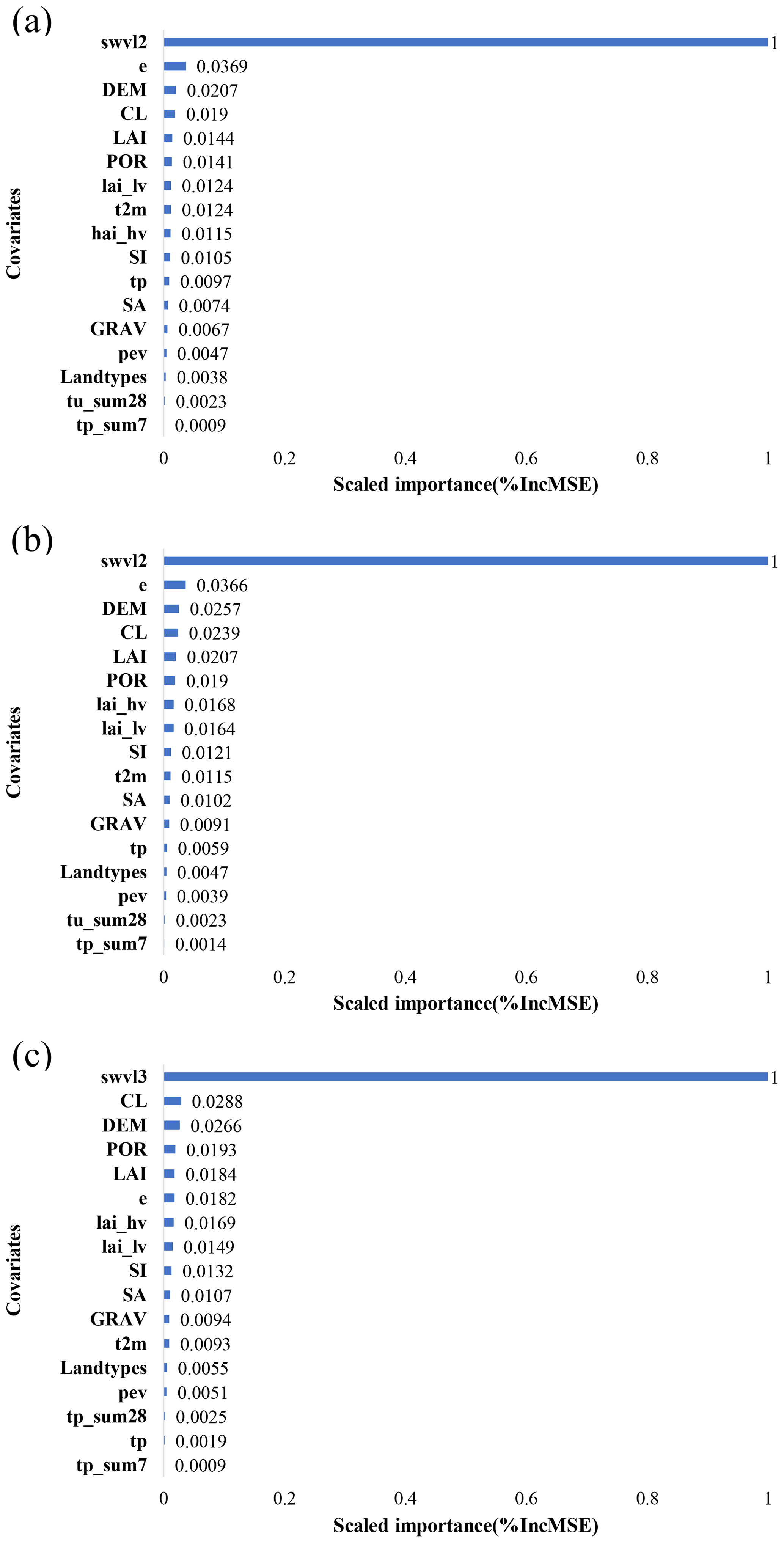
Figure 8Relative importance of predictors for the random forest (RF) model at soil depths of (a) 10 cm, (b) 20 cm, and (c) 30 cm.
4.2 Sensitivity to precipitation, air temperature, and radiation
We applied partial correlation to analyze the sensitivity between the meteorological variables (precipitation, air temperature, and radiation) and SM data. As Fig. 9 shows, precipitation had a stronger correlation with SM in SMCI1.0 and ERA5-Land data than that in the SoMo.ml product across most regions in China, presenting significant positive partial correlations. Additionally, air temperature had a significant positive partial correlation with SM in northwestern China and negative partial correlations in northern China and Liaoning Province (118∘53′ E–125∘46′ E, 38∘43′ N–43∘26′ N) for SMCI1.0. The negative partial correlation between air temperature and SM is consistent with the physics of the process that higher evaporation is caused by higher air temperatures, leading to lower SM. In some of the plateau areas (73∘19′ E–104∘47′ E, 26∘00′ N–39∘47′ N), the shortwave radiation is the dominant factor in SM variability for the SMCI1.0 product, physically sound logic that the strong radiation in the plateau area has a great impact on the land surface process. Meanwhile, we also found that the shortwave radiation has a great influence on the SM variability in tropical monsoon climate regions, which is also consistent with the previous study (Yao et al., 2011). The negative correlation between radiation and SM for the SoMo.ml product in the temperature climate region was stronger than that for the SMCI1.0 product, which could explain more negative trends in SM in the temperature climate region for the SoMo.ml product. Compared with the other SM products, the SMCI1.0 dataset shows similar spatial patterns for all the partial correlations. Overall, the SMCI1.0 product provides reasonable results in reflecting the relationship between SM and its related meteorological variables.
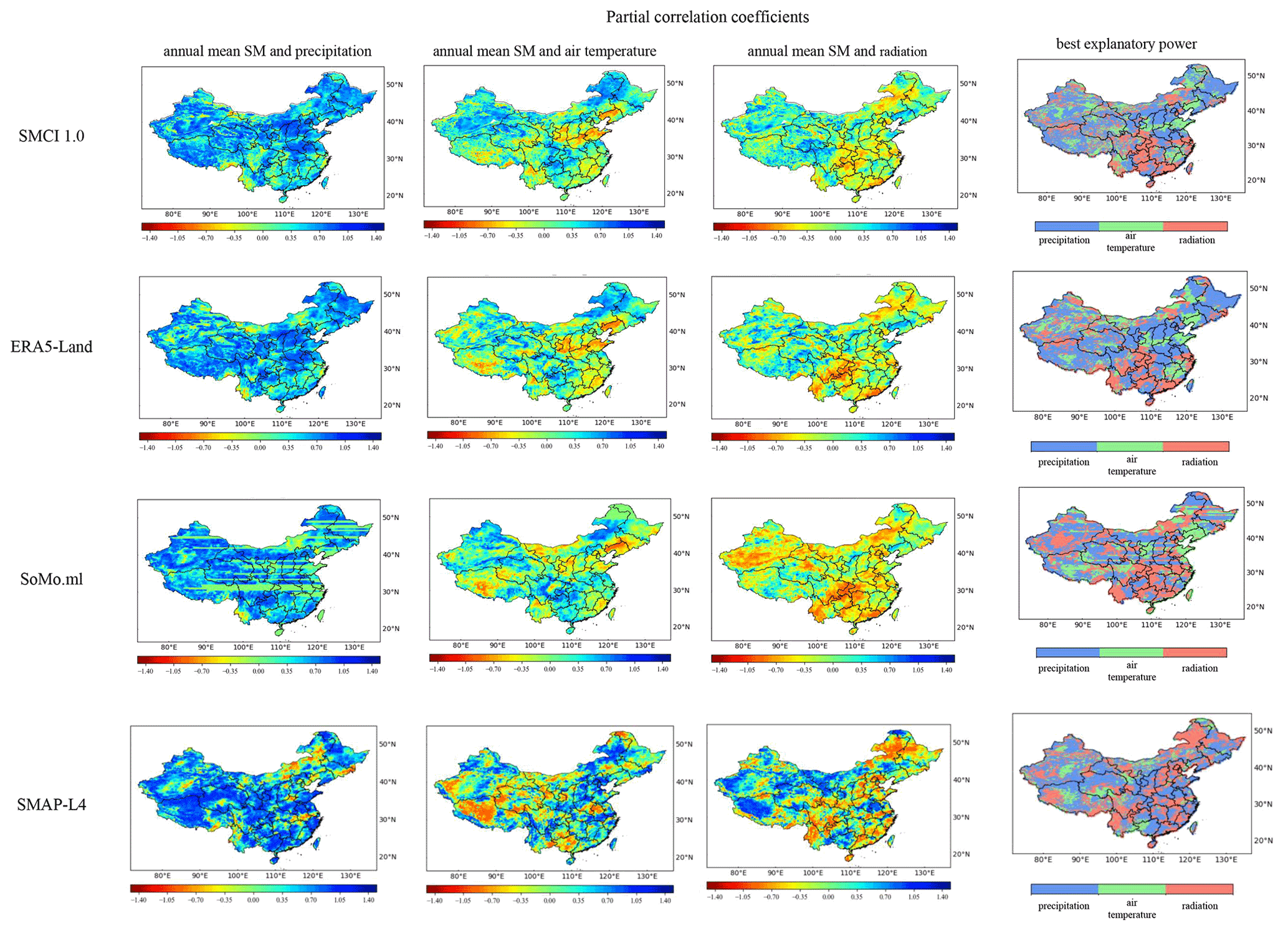
Figure 9Partial correlation coefficients between annual mean SM and precipitation (the first column), air temperature (the second column), and radiation (the third column) for the different gridded SM products. The fourth column represents the best explanatory power (highest absolute partial correlation) for the interannual variability in SM for the different gridded SM products.
4.3 Factors affecting the quality of the SMCI1.0 dataset
Figures 2 and S2 show that SM results at 70 and 90 cm were significantly worse than those at other depths. The reason may be that linked to the inability of the RF model to estimate accurate SM when data from only a few in situ SM stations are available. From Fig. S1b, we can see that the total number of data at 70 and 90 cm soil depths are quite small. In other words, more abundant data could help the RF model to “learn” relationships between predictors and in situ SM data reliably and further improve the quality of high-resolution SM estimation over China. Meanwhile, compared with the previous study of O and Orth (2021), our SMCI1.0 showed the superior quality (Figs. 4–6), because the larger numbers of in situ SM data of China were applied for the RF-based modeling.
From Fig. 5, during the rainfall near the 91st day across the tropical monsoon climate zone (Am) and near the 1st day across the snow climate with a dry winter zone (Dw), the in situ SM values did not increase due to high precipitation, but the SMCI1.0 product could capture the increase in SM (denoted in the light blue rectangle). The reason may be that the applied predictors had a bias with in situ measurements and further affected the SM estimation by the RF model. Meanwhile, we also found that the RF model could overcome much bias in dry conditions, except for those from the 196th to 305th days in the snow climate and fully humid zone (shown in the light red rectangle). In the case of 30 cm soil depth (Fig. S5), we could see an agreement between several peak events that could be attributed to the soil texture homogeneity at the 10 and 30 cm soil depths. Almost all climatic regions had lower dynamic ranges at 30 cm soil depth than that at 10 cm, and this may be attributed to the persistent behavior of SM at 30 cm soil depth. In the case of the 30 cm soil depth in Fig. S6, the SMCI1.0 product had a higher accuracy than that at 10 cm soil depth (Fig. 6), especially in terms of ubRMSE and MAE metrics. The reason may be the background aridity, which could lead to low variability of SM in the deeper layers (Karthikeyan and Mishra 2021), so that the RF model could capture the SM variation in SM straightforwardly.
In contrast, it is inconsistent for the results of R, ubRMSE, and MAE in Figs. 2 and 4, which is similar to the previous study (Sungmin and Orth, 2020) (represented in their Figs. 4 and 5). For example, the SMCI1.0 product led to the ubRMSE, MAE, and R values being 0.046, 0.035, and 0.889 at 10 cm soil depth in Fig. 2. However, in Fig. 4, the box plot shows the lowest ubRMSE and MAE and highest R values of the SMCI1.0 product as 0.03, 0.02, and 0.7, respectively. The reason may be the circumstances of computing the same metrics in different ways, so that the results of Fig. 2 are for all stations and temporal periods, whereas Fig. 4 shows the results of the temporal period at only one station.
The results obtained by the RF method were also compared with those of some other ML models, including the CatBoost (Dorogush et al., 2018), XgBoost (Chen and Guestrin, 2016), and Neural Network (Rosenblatt et al., 1958) models. We found that their performance is similar to RF models with a R2 value of around 0.79. Therefore, due to the comparable performance and wide application of RF to SM modeling (e.g., Carranza et al., 2021; Lin and Liu, 2022; Ly et al., 2021) and more importantly due to its cost-effective runtime, only the results of RF were considered to produce high-resolution SM data in this study.
4.4 Requirement of further validations and improvements
The SMCI1.0 product generally agrees well with in situ SM data over China with regard to other considered datasets in the year-to-year and station-to-station validation scenarios. However, we cannot ensure the same quality over different parts of China. The reason is that in situ SM stations are unevenly distributed over China, with higher sparsity in the west. We hope that more in situ SM stations will be evenly deployed in China, where such data could improve the quality of SM in most regions as far as possible. Triple collocation analysis (Karthikeyan and Mishra, 2021) is also an alternative method for evaluating the SMCI1.0 product. Meanwhile, there are many possible reasons for the failure of the RF model, such as a lack of sufficient data and the weak “learning” of the model itself. Hence, not only additional records from China need to be available, but more robustly estimated models may also be proposed and used for SM modeling. For instance, the deep learning models can be built and optimized for different homogeneous regions (Karthikeyan and Mishra, 2021), or the optical remote sensing can be used for the human-induced regions (Chen et al., 2021), which may lead to better estimation of SM.
It is well known that higher-resolution (<1 km) SM estimation is typically considered a complex and challenging task (Peng et al., 2021). The relatively important predictors identified in Sect. 4.1 can enhance the modeling performance and generated data quality of the higher-resolution SM product. The SMCI1.0 product may also be used as a vital predictor for improving the higher-resolution SM products. Moreover, downscaling to the higher-resolution SM product based on the lower-resolution predictors can also be considered a super-resolution task in computer science, and the advanced deep learning models can also be explored (Lei et al., 2020; H. Zhang et al., 2021; Zhu et al., 2022).
4.5 Comparison with previous products and implications for the soil moisture modeling
This section mainly described and discussed the comparison between SMCI1.0 and some other SM products and the implications for the soil moisture modeling and attribution. From the results presented in Sect. 3, we can see that SMCI1.0 generally outperforms some other SM products (e.g., ERA5-Land, SoMo.ml, and SMAP-L4) in most cases. The most important uniqueness of SMCI1.0 is its taking the in situ SM data as the training target with abundant sample size. Even though we used ERA5-Land to correct their means and standard deviation at each site, the temporal variation still came from the point observations. We have also examined the RF model training with the original SM observations and found that the performance of the model is much worse, with a R2 of 0.67 compared with the model, with a correction with a R2 of 0.79. More importantly, the resulting SM maps demonstrated an unreasonably noisy spatial distribution. This indicates that the in situ SM in China has a fundamental data inconsistency, and the correction according to ERA5-Land is necessary, which has physical consistency. Furthermore, SMCI1.0 has been provided with relatively high spatial and temporal resolutions (1 km, daily) for 10 soil depths, which makes it possible for wider applications at finer scales and deep soils for the whole of China, while reanalysis and remote sensing SM data are often at a coarser resolution, and remote sensing SM data are only for the surface soil.
As a limitation of SMCI1.0, the machine-learning-based model cannot always reflect the variation of SM well, especially for some extreme events or so-called “tipping points” (Bury et al., 2021). From Fig. 5, we can see that SMCI1.0 deviated from the in situ SM data in some cases, though this also happened to the other three SM products. For example, from the 35th day to the 61st day across the snow climate, fully humid (Df), SMCI1.0 and SoMo.ml overestimated it, while SMAP_L4 underestimated it. Tipping points denoted that a slowly changing SM sparks a sudden shift to a new one (Bury et al., 2021). This discontinuity creates a big challenge for estimating in situ SM by ML models, because tipping points simplify the dynamics of a complex system, down to the limited number of possible “normal forms” (Bury et al., 2021). ML models cannot accurately capture such extreme events. Hence, for these extreme events, we hope that ML models trained on a sufficiently diverse dataset of possible SM variation will capture the complex relationship between SM and predictors well. As a suggestion for future work, a possible solution for this limitation is to apply a land surface model, such as the Common Land Model (Dai et al., 2003), to simulate large numbers of SM data and select the local bifurcations in SM variation as supplementary samples to enhance the learning generality of the RF model.
All resources of the RF model, including the training and testing code, are publicly available at https://github.com/ljz1228/SMCI1.0_RF (last access: 22 November 2022). Data with resolutions of 1 and 9 km can be accessed at http://dx.doi.org/10.11888/Terre.tpdc.272415 (Shangguan et al., 2022).
High-resolution SM has several potential applications in flood and drought prediction and carbon cycle modeling. Currently available SM gridded products covering China or the world are often based on remote sensing data or numerical modeling. However, there is still a lack of SM data with high resolution at multiple layers based on in situ measurements for China. In this study, the gridded SM data were estimated through the RF method over China based on the ERA5-Land reanalysis, USGS land cover type and DEM, and reprocessed LAI and soil properties from the CSDL, which included soil depths from 10 to 100 cm and had a 1 km spatial and daily temporal resolution over the period from 1 January 2010 to 31 December 2020. Two independent experiments with in situ soil moisture as the benchmark were conducted to investigate the quality of SMCI1.0: year-to-year experiment (ubRMSE ranges from 0.041 to 0.052, MAE ranges from 0.03 to 0.036, R ranges from 0.883 to 0.919, and R2 ranges from 0.767 to 0.842) and station-to-station experiment (ubRMSE ranges from 0.045 to 0.051, MAE ranges from 0.035 to 0.038, R ranges from 0.866 to 0.893, and R2 ranges from 0.749 to 0.798). SMCI1.0 generally showed advantages over other gridded SM products, including ERA5-Land, SMAP-L4, and SoMo.ml. Meanwhile, with regard to the agreement statistics (ubRMSE, R, bias, and MAE), we could see that the SMCI1.0 product has relatively low ubRMSE, bias, and MAE values over most regions. However, the high errors of SM obtained were often located in the North China Monsoon Region. Moreover, SMCI1.0 has a reasonable spatial pattern and demonstrates more spatial details compared with the SM products. As a result, the SMCI1.0 product based on in situ data can be useful a complement of existing model-based and satellite-based datasets for various hydrological, meteorological, and ecological analyses and models, especially for those applications requiring high-resolution SM maps. Further works may focus on improving the SM map by using advanced deep learning methods and adding more observations, especially for the western part of China. It is also possible to update and extend the time coverage of this dataset before 2010 as long as in situ SM data become available.
The supplement related to this article is available online at: https://doi.org/10.5194/essd-14-5267-2022-supplement.
WS conceived the research and secured funding for it. QL and WS performed the analyses. QL wrote the first draft of the manuscript. GS and QL conducted the research. WS and QL reviewed and edited the manuscript before submission. WS, QL, and VN revised the manuscript. JL, LL, FH, YZ, CW, DW, JQ, XL, and YD joined the discussion of the research.
The contact author has declared that none of the authors has any competing interests.
Publisher's note: Copernicus Publications remains neutral with regard to jurisdictional claims in published maps and institutional affiliations.
The authors are grateful to all the data contributors who made it possible to complete this research.
The study was partially supported by the National Natural Science Foundation of China (grant nos. 41975122, 42105144, 4227515, 42205149, and U1811464) and the National Key Research and Development Program of China under grant no. 2017YFA0604303.
This paper was edited by Hanqin Tian and reviewed by three anonymous referees.
Albertson, J. D. and Kiely, G.: On the structure of soil moisture time series in the context of land surface models, J. Hydrol., 243, 101–119, https://doi.org/10.1016/S0022-1694(00)00405-4, 2001.
Balenović, I., Marjanović, H., Vuletić, D., Paladinić, E., and Indir, K.: Quality assessment of high density digital surface model over different land cover classes, Period. Biol., 117, 459–470, https://doi.org/10.18054/pb.2015.117.4.3452, 2016.
Balsamo, G., Albergel, C., Beljaars, A., Boussetta, S., Brun, E., Cloke, H., Dee, D., Dutra, E., Muñoz-Sabater, J., Pappenberger, F., de Rosnay, P., Stockdale, T., and Vitart, F.: ERA-Interim/Land: a global land surface reanalysis data set, Hydrol. Earth Syst. Sci., 19, 389–407, https://doi.org/10.5194/hess-19-389-2015, 2015.
Baroni, G., Ortuani, B., Facchi, A., and Gandolfi, C.: The role of vegetation and soil properties on the spatio-temporal variability of the surface soil moisture in a maize-cropped field, J. Hydrol., 489, 148–159, https://doi.org/10.1016/j.jhydrol.2013.03.007, 2013.
Breiman, L.: Random Forests, Machine Learning, 45, 5–32, https://doi.org/10.1023/A:1010933404324, 2001.
Brocca, L., Morbidelli, R., Melone, F., and Moramarco, T.: Soil moisture spatial variability in experimental areas of central Italy, J. Hydrol., 333, 356–373, https://doi.org/10.1016/j.jhydrol.2006.09.004, 2007.
Bury, T. M., Sujith, R. I., Pavithran, I., Scheffer, M., Lenton, T. M., Anand, M., and Bauch, C. T.: Deep learning for early warning signals of tipping points, P. Natl. Acad. Sci., 118, e2106140118, https://doi.org/10.1073/pnas.2106140118, 2021.
Carranza, C., Nolet, C., Pezij, M., and van der Ploeg, M.: Root zone soil moisture estimation with Random Forest, J. Hydrol., 593, 125840, https://doi.org/10.1016/j.jhydrol.2020.125840, 2021.
Chakrabarti, S., Bongiovanni, T., Judge, J., Nagarajan, K., and Principe, J. C.: Downscaling Satellite-Based Soil Moisture in Heterogeneous Regions Using High-Resolution Remote Sensing Products and Information Theory: A Synthetic Study, IEEE T. Geosci. Remote, 53, 85–101, https://doi.org/10.1109/TGRS.2014.2318699, 2015.
Chawla, I., Karthikeyan, L., and Mishra, A. K.: A review of remote sensing applications for water security: Quantity, quality, and extremes, J. Hydrol., 585, 124826, https://doi.org/10.1016/j.jhydrol.2020.124826, 2020.
Chen, M., Willgoose, G. R., and Saco, P. M.: Investigating the impact of leaf area index temporal variability on soil moisture predictions using remote sensing vegetation data, J. Hydrol., 522, 274–284, https://doi.org/10.1016/j.jhydrol.2014.12.027, 2015.
Chen, T. and Guestrin, C.: XGBoost: A Scalable Tree Boosting System, in Proceedings of the 22nd ACM SIGKDD international conference on knowledge discovery and data mining, USA, 13–17 August 2016, 785–794, https://doi.org/10.1145/2939672.2939785, 2016.
Chen, Y., Feng, X., and Fu, B.: An improved global remote-sensing-based surface soil moisture (RSSSM) dataset covering 2003–2018, Earth Syst. Sci. Data, 13, 1–31, https://doi.org/10.5194/essd-13-1-2021, 2021.
Cong, N., Wang, T., Nan, H., Ma, Y., Wang, X., Myneni, R. B., and Piao, S.: Changes in satellite-derived spring vegetation green-up date and its linkage to climate in China from 1982 to 2010: a multimethod analysis, Glob. Change Biol., 19, 881–891, https://doi.org/10.1111/gcb.12077, 2013.
Crow, W. T., Berg, A. A., Cosh, M. H., Loew, A., Mohanty, B. P., Panciera, R., de Rosnay, P., Ryu, D., and Walker, J. P.: Upscaling sparse ground-based soil moisture observations for the validation of coarse-resolution satellite soil moisture products, Rev. Geophys., 50, RG2002, https://doi.org/10.1029/2011RG000372, 2012.
Dai, Y., Zeng, X., Dickinson, R. E., Baker, I., Bonan, G. B., Bosilovich, M. G., Denning, A. S., Dirmeyer, P. A., Houser, P. R., Niu, G., Oleson, K. W., Schlosser, C. A., and Yang, Z.-L.: The Common Land Model, B. Am. Meteorol. Soc., 84, 1013–1024, https://doi.org/10.1175/BAMS-84-8-1013, 2003.
Dirmeyer, P. A., Gao, X., Zhao, M., Guo, Z., Oki, T., and Hanasaki, N.: GSWP-2: Multimodel Analysis and Implications for Our Perception of the Land Surface, B. Am. Meteorol. Soc., 87, 1381–1398, https://doi.org/10.1175/BAMS-87-10-1381, 2006.
Dorigo, W. A., Xaver, A., Vreugdenhil, M., Gruber, A., Hegyiová, A., Sanchis-Dufau, A. D., Zamojski, D., Cordes, C., Wagner, W., and Drusch, M.: Global Automated Quality Control of In Situ Soil Moisture Data from the International Soil Moisture Network, Vadose Zone J., 12, vzj2012.0097, https://doi.org/10.2136/vzj2012.0097, 2013.
Dorogush, A. V., Ershov, V., and Gulin, A.: CatBoost: gradient boosting with categorical features support, arXiv [preprint], https://doi.org/10.48550/arXiv.1810.11363, 24 October 2018.
Entekhabi, D., Rodriguez-Iturbe, I., and Castelli, F.: Mutual interaction of soil moisture state and atmospheric processes, J. Hydrol., 184, 3–17, https://doi.org/10.1016/0022-1694(95)02965-6, 1996.
Entekhabi, D., Njoku, E. G., Neill, P. E. O., Kellogg, K. H., Crow, W. T., Edelstein, W. N., Entin, J. K., Goodman, S. D., Jackson, T. J., Johnson, J., Kimball, J., Piepmeier, J. R., Koster, R. D., Martin, N., McDonald, K. C., Moghaddam, M., Moran, S., Reichle, R., Shi, J. C., Spencer, M. W., Thurman, S. W., Tsang, L., and Zyl, J. V.: The Soil Moisture Active Passive (SMAP) Mission, P. IEEE, 98, 704–716, https://doi.org/10.1109/JPROC.2010.2043918, 2010.
Feng, H. and Liu, Y.: Combined effects of precipitation and air temperature on soil moisture in different land covers in a humid basin, J. Hydrol., 531, 1129–1140, https://doi.org/10.1016/j.jhydrol.2015.11.016, 2015.
Fujii, H., Koike, T., and Imaoka, K.: Improvement of the AMSR-E Algorithm for Soil Moisture Estimation by Introducing a Fractional Vegetation Coverage Dataset Derived from MODIS Data, Journal of the Remote Sensing Society of Japan, 29, 282–292, https://doi.org/10.11440/rssj.29.282, 2009.
Gaur, N. and Mohanty, B. P.: Land-surface controls on near-surface soil moisture dynamics: Traversing remote sensing footprints, Water Resour. Res., 52, 6365–6385, https://doi.org/10.1002/2015WR018095, 2016.
Global Climate Observing System (GCOS): The Global Observing System for Climate: Implementation Needs, World Meteorological Organization, Guayaquil, Ecuador, Rep. GCOS-200, 341 pp., https://doi.org/10.13140/RG.2.2.23178.26566, 2016.
Gruber, A., Su, C. H., Crow, W. T., Zwieback, S., Dorigo, W. A., and Wagner, W.: Estimating error cross-correlations in soil moisture data sets using extended collocation analysis, J. Geophys. Res.-Atmos., 121, 1208–1219, https://doi.org/10.1002/2015JD024027, 2016.
Gu, X., Li, J., Chen, Y. D., Kong, D., and Liu, J.: Consistency and Discrepancy of Global Surface Soil Moisture Changes from Multiple Model-Based Data Sets Against Satellite Observations, J. Geophys. Res.-Atmos., 124, 1474–1495, https://doi.org/10.1029/2018JD029304, 2019.
Guo, L. and Lin, H.: Chapter Two – Addressing Two Bottlenecks to Advance the Understanding of Preferential Flow in Soils, in: Advances in Agronomy, edited by: Sparks, D. L., Academic Press, 61–117, https://doi.org/10.1016/bs.agron.2017.10.002, 2018.
Hu, Q. and Feng, S.: A Daily Soil Temperature Dataset and Soil Temperature Climatology of the Contiguous United States, J. Appl. Meteorol., 42, 1139–1156, https://doi.org/10.1175/1520-0450(2003)042<1139:ADSTDA>2.0.CO;2, 2003.
Joshi, C. and Mohanty, B. P.: Physical controls of near-surface soil moisture across varying spatial scales in an agricultural landscape during SMEX02, Water Resour. Res., 46, W12503, https://doi.org/10.1029/2010WR009152, 2010.
Karthikeyan, L. and Kumar, D. N.: A novel approach to validate satellite soil moisture retrievals using precipitation data, J. Geophys. Res.-Atmos., 121, 11516–11535, https://doi.org/10.1002/2016JD024829, 2016.
Karthikeyan, L. and Mishra, A. K.: Multi-layer high-resolution soil moisture estimation using machine learning over the United States, Remote Sens. Environ., 266, 112706, https://doi.org/10.1016/j.rse.2021.112706, 2021.
Kemppinen, J., Niittynen, P., Virkkala, A.-M., Happonen, K., Riihimäki, H., Aalto, J., and Luoto, M.: Dwarf Shrubs Impact Tundra Soils: Drier, Colder, and Less Organic Carbon, Ecosystems, 24, 1378–1392, https://doi.org/10.1007/s10021-020-00589-2, 2021.
Kerr, Y. H., Waldteufel, P., Wigneron, J., Delwart, S., Cabot, F., Boutin, J., Escorihuela, M., Font, J., Reul, N., Gruhier, C., Juglea, S. E., Drinkwater, M. R., Hahne, A., Martín-Neira, M., and Mecklenburg, S.: The SMOS Mission: New Tool for Monitoring Key Elements ofthe Global Water Cycle, P. IEEE, 98, 666–687, https://doi.org/10.1109/JPROC.2010.2043032, 2010.
Kim, S., Zhang, R., Pham, H., and Sharma, A.: A Review of Satellite-Derived Soil Moisture and Its Usage for Flood Estimation, Remote Sensing in Earth Systems Sciences, 2, 225–246, https://doi.org/10.1007/s41976-019-00025-7, 2019.
Kumar, S. V., Reichle, R. H., Koster, R. D., Crow, W. T., and Peters-Lidard, C. D.: Role of Subsurface Physics in the Assimilation of Surface Soil Moisture Observations, J. Hydrometeorol., 10, 1534–1547, https://doi.org/10.1175/2009JHM1134.1, 2009.
Le Bissonnais, Y., Renaux, B., and Delouche, H.: Interactions between soil properties and moisture content in crust formation, runoff and interrill erosion from tilled loess soils, CATENA, 25, 33–46, https://doi.org/10.1016/0341-8162(94)00040-L, 1995.
Lei, S., Shi, Z., and Zou, Z.: Coupled Adversarial Training for Remote Sensing Image Super-Resolution, IEEE T. Geosci. Remote, 58, 3633–3643, https://doi.org/10.1109/TGRS.2019.2959020, 2020.
Li, L., Shangguan, W., Deng, Y., Mao, J., Pan, J., Wei, N., Yuan, H., Zhang, S., Zhang, Y., and Dai, Y.: A Causal Inference Model Based on Random Forests to Identify the Effect of Soil Moisture on Precipitation, J. Hydrometeorol., 21, 1115–1131, https://doi.org/10.1175/JHM-D-19-0209.1, 2020.
Li, Q., Wang, Z., Shangguan, W., Li, L., Yao, Y., and Yu, F.: Improved daily SMAP satellite soil moisture prediction over China using deep learning model with transfer learning, J. Hydrol., 600, 126698, https://doi.org/10.1016/j.jhydrol.2021.126698, 2021.
Lin, L. and Liu, X.: Mixture-based weight learning improves the random forest method for hyperspectral estimation of soil total nitrogen, Comput. Electron. Agr., 192, 106634, https://doi.org/10.1016/j.compag.2021.106634, 2022.
Loveland, T. R., Reed, B. C., Brown, J. F., Ohlen, D. O., Zhu, Z., Yang, L., and Merchant, J. W.: Development of a global land cover characteristics database and IGBP DISCover from 1 km AVHRR data, Int. J. Remote Sens. 21, 1303–1330, https://doi.org/10.1080/014311600210191, 2000.
Ly, H. B., Nguyen, T. A., and Pham, B. T.: Estimation of Soil Cohesion Using Machine Learning Method: A Random Forest Approach, Advances in Civil Engineering, 2021, 8873993, https://doi.org/10.1155/2021/8873993, 2021.
Mao, T., Shangguan, W., Li, Q., Li, L., Zhang, Y., Huang, F., Li, J., Liu, W., and Zhang, R.: A Spatial Downscaling Method for Remote Sensing Soil Moisture Based on Random Forest Considering Soil Moisture Memory and Mass Conservation, Remote Sensing, 14, 3858, https://doi.org/10.3390/rs14163858, 2022.
Meng, X., Mao, K., Meng, F., Shi, J., Zeng, J., Shen, X., Cui, Y., Jiang, L., and Guo, Z.: A fine-resolution soil moisture dataset for China in 2002–2018, Earth Syst. Sci. Data, 13, 3239–3261, https://doi.org/10.5194/essd-13-3239-2021, 2021.
Mishra, A., Vu, T., Veettil, A. V., and Entekhabi, D.: Drought monitoring with soil moisture active passive (SMAP) measurements, J. Hydrol., 552, 620–632, https://doi.org/10.1016/j.jhydrol.2017.07.033, 2017.
Mohamed, E., Habib, E., Abdelhameed, A. M., and Bayoumi, M.: Assessment of a Spatiotemporal Deep Learning Approach for Soil Moisture Prediction and Filling the Gaps in Between Soil Moisture Observations, Frontiers in Artificial Intelligence, 4, 636234, https://doi.org/10.3389/frai.2021.636234, 2021.
Muñoz Sabater, J.: ERA5-Land hourly data from 1981 to present, Copernicus Climate Change Service (C3S) Climate Data Store (CDS) [data set], https://doi.org/10.24381/cds.e2161bac, 2019.
Muñoz Sabater, J.: ERA5-Land hourly data from 1950 to 1980, Copernicus Climate Change Service (C3S) Climate Data Store (CDS) [data set], https://doi.org/10.24381/cds.e2161bac, 2021.
Muñoz-Sabater, J., Dutra, E., Agustí-Panareda, A., Albergel, C., Arduini, G., Balsamo, G., Boussetta, S., Choulga, M., Harrigan, S., Hersbach, H., Martens, B., Miralles, D. G., Piles, M., Rodríguez-Fernández, N. J., Zsoter, E., Buontempo, C., and Thépaut, J.-N.: ERA5-Land: a state-of-the-art global reanalysis dataset for land applications, Earth Syst. Sci. Data, 13, 4349–4383, https://doi.org/10.5194/essd-13-4349-2021, 2021.
Norbiato, D., Borga, M., Degli Esposti, S., Gaume, E., and Anquetin, S.: Flash flood warning based on rainfall thresholds and soil moisture conditions: An assessment for gauged and ungauged basins, J. Hydrol., 362, 274–290, https://doi.org/10.1016/j.jhydrol.2008.08.023, 2008.
O, S. and Orth, R.: Global soil moisture data derived through machine learning trained with in-situ measurements, Scientific Data, 8, 170, https://doi.org/10.1038/s41597-021-00964-1, 2021.
Ojha, R., Morbidelli, R., Saltalippi, C., Flammini, A., and Govindaraju, R. S.: Scaling of surface soil moisture over heterogeneous fields subjected to a single rainfall event, J. Hydrol., 516, 21–36, https://doi.org/10.1016/j.jhydrol.2014.01.057, 2014.
Orth, R. and Seneviratne, S. I.: Using soil moisture forecasts for sub-seasonal summer temperature predictions in Europe, Clim. Dynam., 43, 3403–3418, https://doi.org/10.1007/s00382-014-2112-x, 2014.
Pan, J., Shangguan, W., Li, L., Yuan, H., Zhang, S., Lu, X., Wei, N., and Dai, Y.: Using data-driven methods to explore the predictability of surface soil moisture with FLUXNET site data, Hydrol. Process., 33, 2978–2996, https://doi.org/10.1002/hyp.13540, 2019.
Parinussa, R. M., Lakshmi, V., Johnson, F. M., and Sharma, A.: A new framework for monitoring flood inundation using readily available satellite data, Geophys. Rese. Lett., 43, 2599–2605, https://doi.org/10.1002/2016GL068192, 2016.
Peng, J., Albergel, C., Balenzano, A., Brocca, L., Cartus, O., Cosh, M. H., Crow, W. T., Dabrowska-Zielinska, K., Dadson, S., Davidson, M. W. J., de Rosnay, P., Dorigo, W., Gruber, A., Hagemann, S., Hirschi, M., Kerr, Y. H., Lovergine, F., Mahecha, M. D., Marzahn, P., Mattia, F., Musial, J. P., Preuschmann, S., Reichle, R. H., Satalino, G., Silgram, M., van Bodegom, P. M., Verhoest, N. E. C., Wagner, W., Walker, J. P., Wegmüller, U., and Loew, A.: A roadmap for high-resolution satellite soil moisture applications – confronting product characteristics with user requirements, Remote Sens. Environ., 252, 112162, https://doi.org/10.1016/j.rse.2020.112162, 2021.
Rosenblatt, F.: The perceptron: A probabilistic model for information storage and organization in the brain, Psychol. Rev., 65, 386–408, https://doi.org/10.1037/h0042519, 1958.
Seneviratne, S. I., Corti, T., Davin, E. L., Hirschi, M., Jaeger, E. B., Lehner, I., Orlowsky, B., and Teuling, A. J.: Investigating soil moisture–climate interactions in a changing climate: A review, Earth-Sci. Rev., 99, 125–161, https://doi.org/10.1016/j.earscirev.2010.02.004, 2010.
Shangguan, W., Dai, Y., Liu, B., Zhu, A., Duan, Q., Wu, L., Ji, D., Ye, A., Yuan, H., Zhang, Q., Chen, D., Chen, M., Chu, J., Dou, Y., Guo, J., Li, H., Li, J., Liang, L., Liang, X., Liu, H., Liu, S., Miao, C., and Zhang, Y.: A China data set of soil properties for land surface modeling, J. Adv. Model. Earth Sy., 5, 212–224, https://doi.org/10.1002/jame.20026, 2013.
Shangguan, W., Li, Q., and Shi, G.: A 1-km daily soil moisture dataset over China based on in-situ measurement (2000–2020), National Tibetan Plateau Data Center [data set], https://doi.org/10.11888/Terre.tpdc.272415, 2022.
Srivastava, P. K., Han, D., Ramirez, M. R., and Islam, T.: Machine Learning Techniques for Downscaling SMOS Satellite Soil Moisture Using MODIS Land Surface Temperature for Hydrological Application, Water Resour. Manag., 27, 3127–3144, https://doi.org/10.1007/s11269-013-0337-9, 2013.
Tijdeman, E. and Menzel, L.: The development and persistence of soil moisture stress during drought across southwestern Germany, Hydrol. Earth Syst. Sci., 25, 2009–2025, https://doi.org/10.5194/hess-25-2009-2021, 2021.
Vereecken, H., Huisman, J. A., Pachepsky, Y., Montzka, C., van der Kruk, J., Bogena, H., Weihermüller, L., Herbst, M., Martinez, G., and Vanderborght, J.: On the spatio-temporal dynamics of soil moisture at the field scale, J. Hydrol., 516, 76–96, https://doi.org/10.1016/j.jhydrol.2013.11.061, 2014.
Wagner, W., Blöschl, G., Pampaloni, P., Calvet, J.-C., Bizzarri, B., Wigneron, J.-P., and Kerr, Y.: Operational readiness of microwave remote sensing of soil moisture for hydrologic applications, Hydrol. Res., 38, 1–20, https://doi.org/10.2166/nh.2007.029, 2007.
Wang, Y., Mao, J., Jin, M., Hoffman, F. M., Shi, X., Wullschleger, S. D., and Dai, Y.: Development of observation-based global multilayer soil moisture products for 1970 to 2016, Earth Syst. Sci. Data, 13, 4385–4405, https://doi.org/10.5194/essd-13-4385-2021, 2021.
Wei, Z., Meng, Y., Zhang, W., Peng, J., and Meng, L.: Downscaling SMAP soil moisture estimation with gradient boosting decision tree regression over the Tibetan Plateau, Remote Sens. Environ., 225, 30–44, https://doi.org/10.1016/j.rse.2019.02.022, 2019.
Xu, J. W., Zhao, J. F., Zhang, W. C., and Xu, X. X.: A Novel Soil Moisture Predicting Method Based on Artificial Neural Network and Xinanjiang Model, Adv. Mat. Res., 121–122, 1028–1032, https://doi.org/10.4028/www.scientific.net/AMR.121-122.1028, 2010.
Yao, Y., Qin, Q., Zhao, S., and Yuan, W.: Retrieval of soil moisture based on MODIS shortwave infrared spectral feature, J. Infrared Millim. Waves, 30, 9–14, http://journal.sitp.ac.cn/hwyhmb/hwyhmben/article/abstract/100118 (last access: 25 November 2022), 2011.
Yuan, H., Dai, Y., Xiao, Z., Ji, D., and Shangguan, W.: Reprocessing the MODIS Leaf Area Index products for land surface and climate modelling, Remote Sens. Environ., 115, 1171–1187, https://doi.org/10.1016/j.rse.2011.01.001, 2011.
Zeng, L., Hu, S., Xiang, D., Zhang, X., Li, D., Li, L., and Zhang, T.: Multilayer Soil Moisture Mapping at a Regional Scale from Multisource Data via a Machine Learning Method, Remote Sensing, 11, 284, https://doi.org/10.3390/rs11030284, 2019.
Zhang, H., Wang, P., and Jiang, Z.: Nonpairwise-Trained Cycle Convolutional Neural Network for Single Remote Sensing Image Super-Resolution, IEEE T. Geosci. Remote, 59, 4250–4261, https://doi.org/10.1109/TGRS.2020.3009224, 2021.
Zhang, Q., Yuan, Q., Li, J., Wang, Y., Sun, F., and Zhang, L.: Generating seamless global daily AMSR2 soil moisture (SGD-SM) long-term products for the years 2013–2019, Earth Syst. Sci. Data, 13, 1385–1401, https://doi.org/10.5194/essd-13-1385-2021, 2021.
Zhang, R., Kim, S., and Sharma, A.: A comprehensive validation of the SMAP Enhanced Level-3 Soil Moisture product using ground measurements over varied climates and landscapes, Remote Sens. Environ., 223, 82–94, https://doi.org/10.1016/j.rse.2019.01.015, 2019.
Zhu, X., Guo, K., Ren, S., Hu, B., Hu, M., and Fang, H.: Lightweight Image Super-Resolution With Expectation-Maximization Attention Mechanism, IEEE T. Circ. Syst. Vid., 32, 1273–1284, https://doi.org/10.1109/TCSVT.2021.3078436, 2022.
Zwieback, S., Chang, Q., Marsh, P., and Berg, A.: Shrub tundra ecohydrology: rainfall interception is a major component of the water balance, Environ. Res. Lett., 14, 055005, https://doi.org/10.1088/1748-9326/ab1049, 2019.