Rescue and quality control of historical geomagnetic measurement at Sheshan observatory, China

The Sheshan Geomagnetic Observatory (International Association of Geomagnetism and Aeronomy (IAGA) code SSH), China was built in Xujiahui, Shanghai in 1874 and moved to Sheshan, Shanghai at the end of 1932. So far, the SSH has a history of nearly 150 years. It is one of the earliest geomagnetic observatories in China and one of the geomagnetic observatories with the longest history in the world. In this paper, we present the rescue and quality control (QC) of the historical data at the SSH from 1933 to 2019. The rescued data are the absolute hourly mean values (AHMVs) of declination (D), horizontal (H), and vertical (Z) components. Some of these data are paper-based records and some are stored in a floppy disk in BAS, DBF, MDB, and other file storage formats. After digitization and format transformation, we imported the data into the Toad database to achieve the unified data management. We performed statistics of completeness, visual analysis, outliers detects, and data correction on the stored data. We then conducted the consistency test of daily variation and secular variation (SV) by comparing the corrected data with the data of the reference observatory, and the computational data of the COV-OBS model, respectively. The consistency test reveals good agreement. However, the individual data should be used with caution because these data are suspicious values, but there is not any explanation or change registered in the available metadata and logbooks. Finally, we present examples of the datasets in discriminating geomagnetic jerks and study of storms. The digitized and quality-controlled AHMVs data are available at: https://doi.org/10.5281/zenodo.7005471 (Zhang et al., 2022).

1 Introduction

Geomagnetic observation data contains abundant solar–terrestrial spatial information, which is widely used in geoscience and space science research. The observation data with time resolutions of 1 s to 1 h are usually used to study various short-period magnetic events such as pulsation, geomagnetic crochet, geomagnetic bay, and magnetic storm (Zhao et al., 2019), and to monitor and predict the electromagnetic environment in solar–terrestrial space. At the same time, it also has important applications in detecting underground electrical structures and evaluating the impact of geomagnetic induced current (GIC) on underground metal pipe network, transmission network, communication cables, high-speed railway lines, and other major projects (Kappenman, 1996; Bolduc et al., 1998, 2002; Boteler et al., 1998; Liu et al., 2008, 2016; Liu et al., 2009; Guo et al., 2015). Observation data with time resolution of 1 h to hundreds of years are usually used for the study of the geomagnetic field and its secular variation (SV), such as geomagnetic jerk (Courtillot and Mouël, 1984; Xu, 2009), magnetic pole movement, dipole magnetic moment change, westward drift, etc., which are of great significance for understanding the material flow inside the core and at the core mantle boundary.

The development and application of geomagnetism depends on long-term data accumulation. The long-term operation of the geomagnetic observatory is very important for the study of the geomagnetic field (Linthe et al., 2013). It is especially valuable to study the variation characteristics of the geomagnetic field from decades to hundreds of years (Clarke et al., 2009; Zhang et al., 2008b). Using the latest scientific and technological means to analyze the continuous geomagnetic observation data as long as possible, to obtain the variation information of the geomagnetic field, has always been a method often used by scientific researchers. However, not all data can be directly provided to researchers, because some data still exist only in the form of hard copy, and even some data face the risk of serious damage and loss due to improper storage conditions. Therefore, it is very important to rescue and digitize these data as soon as possible. High-quality data are the basis of scientific research and the prerequisite for obtaining valuable results (Linthe et al., 2013). Scientists around the world have paid more and more attention to the accumulation of observation data, the rescue of historical data and the sharing of scientific data resources (Curto and Marsal., 2007; Peng et al., 2007; Chulliat et al., 2009; Korte et al., 2009; Dawson et al., 2009; Reay et al., 2013; Morozova et al., 2014, 2021; Sergeyeva et al., 2021; Dong et al., 2009; Zhao et al., 2017; Thomson, 2020).

The rescue, recovery, digitization, and the quality control (QC) of historical geomagnetic data are of extraordinary importance for the geomagnetic community (Rasson et al., 2011). This paper presents the collection, collation, digitization, quality control, and correction of the historical data of the Sheshan Geomagnetic Observatory (International Association of Geomagnetism and Aeronomy code SSH) from 1933 to 2019. The SSH Geomagnetic Observatory is the geomagnetic observatory with the longest history in China. Although many efforts have been made (Gao and Hu, 1993), the existing data are still insufficient. Our work aims at filling the lack of observation data at the SSH observatory since 1933, presenting the data of absolute hourly mean values (AHMVs) collected from 1933 to 2019.

This paper is organized as follows. Section 2 describes the data acquisition method, providing information about SSH observatory history, data sources, and the digitization method. Section 3 introduces the quality control of the digitized data. Section 4 describes the correction of the selected problem data. Section 5 describes the validation of the corrected series by comparing it with reference series and Sect. 6 presents application examples of the datasets. Concluding remarks are given in Sect. 7.

2 Data production methods

2.1 The Sheshan geomagnetic observatory

The first step of the data-rescue process was to collect resources scattered in different locations, which exist in various forms, including data and metadata that may have an influence on data rescue (observatory relocation, instrument replacement, replacement of observers, environmental change, etc.). We have carefully examined the documentation stored in the SSH, Geomagnetic Network of China (GNC), and reference room of the Institute of Geophysics, China Earthquake Administration (IGPCEA). The reference room is a resource center of the IGPCEA, used to collect books, journals, papers, monographs, unpublished reports, internal textbooks, research reports, reference documents, and scientific research achievements related to the discipline. It took us nearly 2 months to collect resources. The documentation consulted includes the Observatory Communication Journal, Geomagnetic Observation Report, Chronicles of China Geomagnetic Observatory, and postal letters. The metadata are mainly stored in the Chronicles of China Geomagnetic Observatory and the Geomagnetic Observation Report. An example of the cover of the bibliographic documents is shown in Fig. 1. The data of 1933–1954 were recorded in the Geomagnetic Observation Report. The observation was interrupted from April 1945 to December 1946 due to World War II. The data of 1955–1994 were stored in the DBF format. The data of 1995–2001 were stored in the BAS format. The data from 2002 to 2006 were stored in the Access database in the MDB format. The DBF, BAS, and MDB are all data file storage formats. The DBF is a tabular data file stored in binary and is the database format used by dBase and FoxPro databases in DOS systems. The BAS file format is written in the BASIC language, a plain-text data storage format. The MDB format is a storage format used by Microsoft Access software that can generally be opened directly with ACCESS. The data of 2007, 2008, and 2010 were lost for unknown reasons. The data from August to December 2011, and July to October 2019 were missed due to the failure of absolute observation instruments. Data for other years from 2009 to 2019 are stored in the Oracle database.

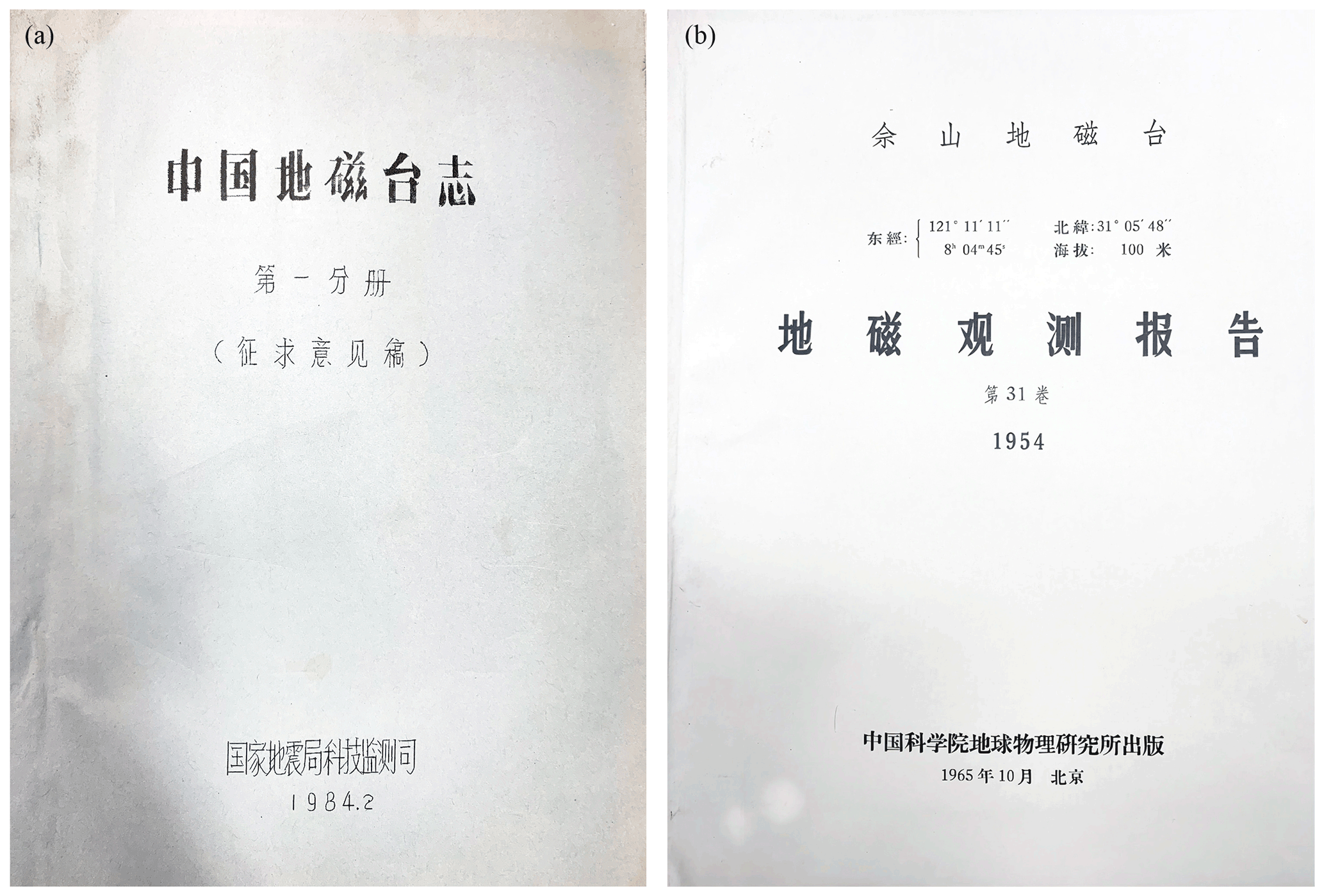
Figure 1 Cover of the (a) Chronicles of China Geomagnetic Observatory (Department of Science, Technology and Monitoring, CEA, 1984) and (b) Geomagnetic Observation Report (Institute of Geophysics, Chinese Academy of Sciences, 1965).

The Sheshan Geomagnetic Observatory (SSH) is presently run by IGPCEA and has been in operation for almost 150 years. Its predecessors are the observatory in Xujiahui, Shanghai, and that in Lujiabang, Jiangsu Province. It was established in Xujiahui in 1874 and began continuous geomagnetic observation since then. It was moved from Xujiahui to Lujiabang in 1908 and then from Lujiabang to Sheshan in December 1932. The Sheshan Geomagnetic Observatory is located in Sheshan (latitude: 31.1^∘ N, longitude: 121.2^∘ E), 20 km to the southwest of Shanghai city. The geology of the vicinity of the observatory is Upper Jurassic to Down Cretaceous Andesite. The gradient of the field is about 2–3 nT m⁻¹. The earliest absolute house and recording room were built in 1932, they are made of non-magnetic material. The regular observation began in 1933.

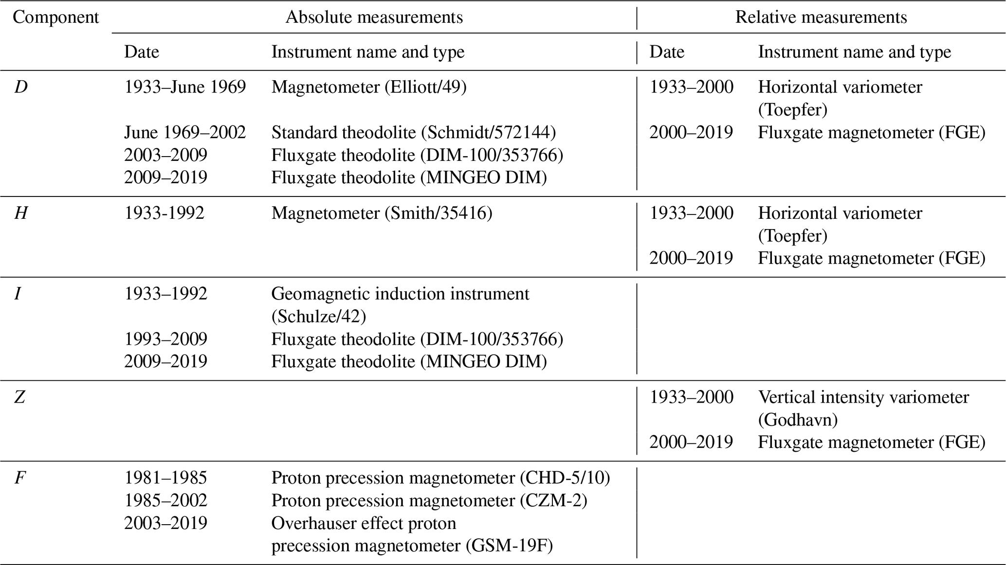
Table 1 shows the absolute and relative instruments in the SSH observatory from 1933 to 2019 and the measured geomagnetic elements at different periods. The information was retrieved from the bibliographic documents mentioned above. The first instrument set included an Elliott (D measurement), a Smith (H measurement), and a Schulze (I measurement) as absolute instruments since 1933. The continuous recordings of magnetic variations of declination (D), horizontal (H), and vertical (Z) were obtained respectively with a horizontal variometer (Toepfer) and a vertical intensity variometer (Godhavn) since 1933. Later, a few replacements of instruments took place in the SSH observatory (Table 1). During this period, many jumps were seen in the relative recorded data due to the adjustment of the variometer, the lightning stroke, earthquakes, and other reasons. These jumps have been corrected by the baseline, so that the absolute value is not affected. By 2000, the SSH observatory was equipped with digital instruments. On 1 January 2003, the Schmidt Standard Theodolite was replaced by a DIM-100/353766 Fluxgate Theodolite and an Overhauser Effect Proton Precession Magnetometer GSM-19F replaced the Proton Precession Magnetometer CZM-2.

Table 1 Summary of instruments in the period from 1933 to 2019 at SSH.

2.2 Data digitization

Because some records are handwritten or manually mimeographed, it is impossible to automate the digitization process. To facilitate the digitization and further application of these records, all the documents were photographed. It is also useful for checking the consistency of digitized data and source data in the future. It is not good for old paper copies to be carried around too much and as soon as we have a digital picture, which is fast to make, we can store the respective papers in their normal archive place again with the usual temperature, humidity, etc. Using the character-recognition program to recognize the photos and compare the consistency with the paper data, it was found that the recognition effect of the character was not ideal. It may be due to the light color of the handwriting, or some of the handwriting is fuzzy and unclear. Therefore, the digitization was mainly performed by key input. We digitized the AHMVs of the three components of declination (D), horizontal (H), and vertical (Z). We designed a set of Excel templates to unify the data-entry format. The digital templates are very similar to the original data source to keep track of our work. The input templates include three workbooks, which are used to store the AHMVs of 1 year, including the AHMVs of the D, H, and Z components. Every AHMVs workbook consists of 14 worksheets, including text description, data worksheets from January to December of every year, and automatic summary worksheets. The monthly data worksheet header includes the station code, measuring point ID, date, large value, and 24 hourly mean values. The large value is a fixed value every month. The purpose of entering a large value is to facilitate the rapid entry of each value. The 24 AHMVs can be calculated by adding the large values to the 24 hourly mean values respectively. For example, the large value in January 1985 was 33 300. For each hourly mean value of this month, we only need to input the digits after thousands' digit. If the input value of 0 h on 1 January was 146.1, we can get the AHMV at this moment by 33 300 plus 146.1, and so on. Missing values were marked as “99 999”. An example of the Excel tables with digitized data is presented in Fig. 2. The “key input” approach is slower but has the lower error rate (Capozzi et al., 2020). After each month of data entry, we cross checked the digitized data with the original source values in order to identify and remove transcription errors. Using this approach, it took us half a year to digitize the 1933–1954 data from paper records.

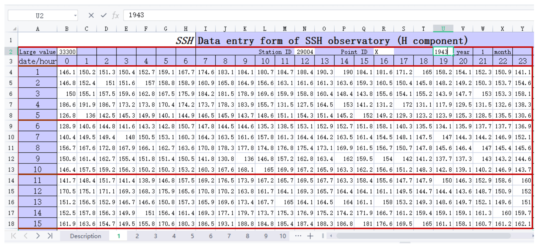
Figure 2 An example of the Excel tables with digitized data.

2.3 Import data stored in various formats into Oracle database

We developed a data convert software (Fig. 3) to import data stored in various formats (XLS, DBF, BAS, and MDB) into a unified Oracle database. In this way, all AHMVs were stored in the same database in a unified format. We call these stored data without any correction the original AHMVs data; it is convenient for the subsequent analysis and application. This allows us to examine the data using Geomagnetic Data Processing Software (GDPST) developed by the Geomagnetic Network of China (Zhang et al., 2016). The GDPST was developed based on the Oracle database. It provides a convenient way of data processing and comparative analysis. The software also has the functions of the data query, data backup, and data download, etc.

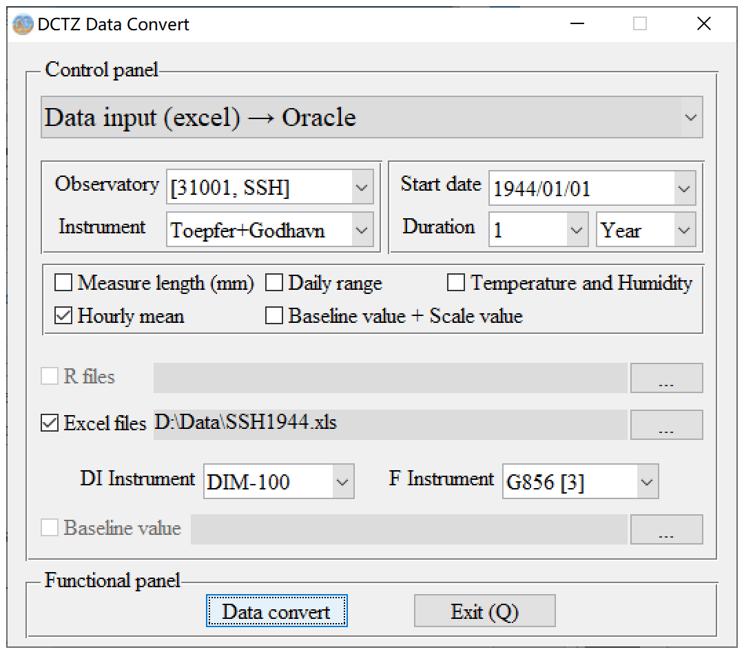
Figure 3 Data import software.

3 Quality control of digitized data of SSH observatory

The purpose of quality control (QC) is to check the completeness and reliability of geomagnetic observation data. The quality of geomagnetic data is often affected by the changes in the instrument or environmental conditions of the measurements, like the repair or re-calibration of the instrument, instrument replacement, observatory relocation, gradual changes of the observation environment, changes in observing process, etc. (Morozova et al., 2014; Zhang et al., 2016). Most such changes can lead to what we call data problems and can be defined as sudden breaks and jumps in the series of geomagnetic data, or gradual biases, or noise and change of transfer function, etc. Correction of problem data before any subsequent analyses is highly desirable (Mestre et al., 2013).

In this study, the QC was performed in order to check the quality of the rescued data. The inspection contents include evaluating the completeness of data, the accuracy of daily variation, the stability of secular variation, and analyzing the influence factors of data quality.

3.1 The completeness of data

Based on the original AHMVs, the annual completeness is calculated using the following Eq. (1):

$$\begin{array}{}\text{(1)}& C=(W_{\mathrm{e}}-W_{\mathrm{m}})/W_{\mathrm{e}},\end{array}$$

where C is the completeness of the AHMVs, W_e is the number of expected data in the chosen period, W_m is the number of missing data, see Fig. 4 for the completeness of data. The series in this study consists of data measured from 1933 to 2019. It has 5 larger gaps with a total of 66 months of data missing; the number of missing data accounts for 6.5 % of the total. All gaps were not replaced by interpolation in this study. War and instrument failure are the main reasons for the gaps of observation.

Figure 4 The completeness of the AHMVs from 1933 to 2019.

3.2 The accuracy of the rescued data

We have designed a strict quality-control procedure to ensure the accuracy of the rescued data. It consists of the following three steps:

1. Preliminary analysis of the series, detection of outliers. In order to avoid the adverse impact of extreme data on the overall trend, we filtered out clearly obvious outliers by the appropriate filtering function of Excel, such as the missing values which were marked as “99 999”, obvious input error, and so on.

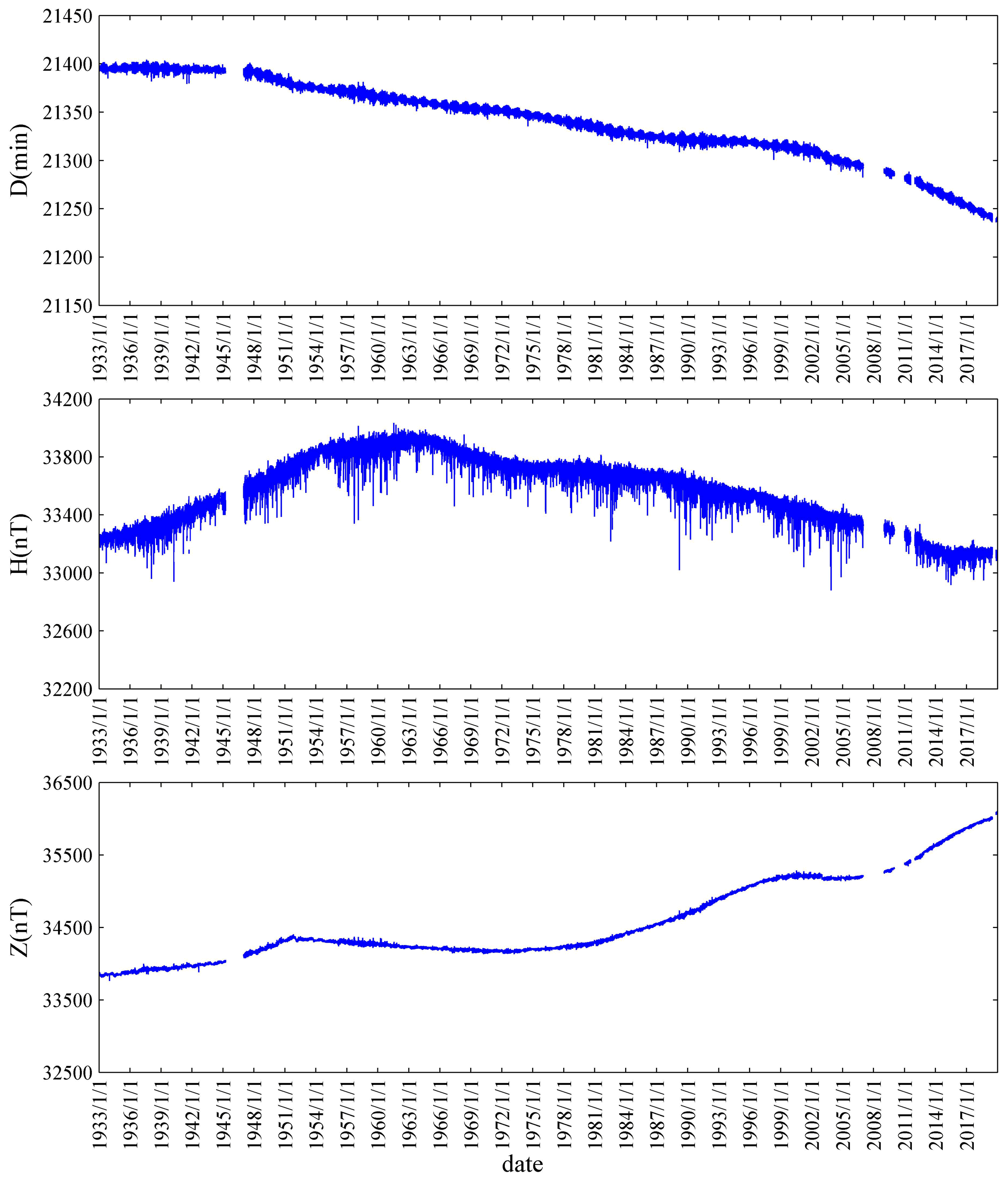
2. Visual analysis of the series and their first-time derivative (FTD) at different timescales. After removing the obvious outliers, we plotted AHMVs of the geomagnetic field components D, H, and Z for all time from 1933 to 2019 (see Fig. 5). It can be seen from the figure that the D, H, and Z components have obvious trends. It is the secular variation (SV) in geomagnetic field with time. The additional signal in the plots mainly comes from the activity of external field. The most significant influence is on both the horizontal components D and H; its influence on the vertical component is minor. In the plots, we do not see obvious step and peak interference.

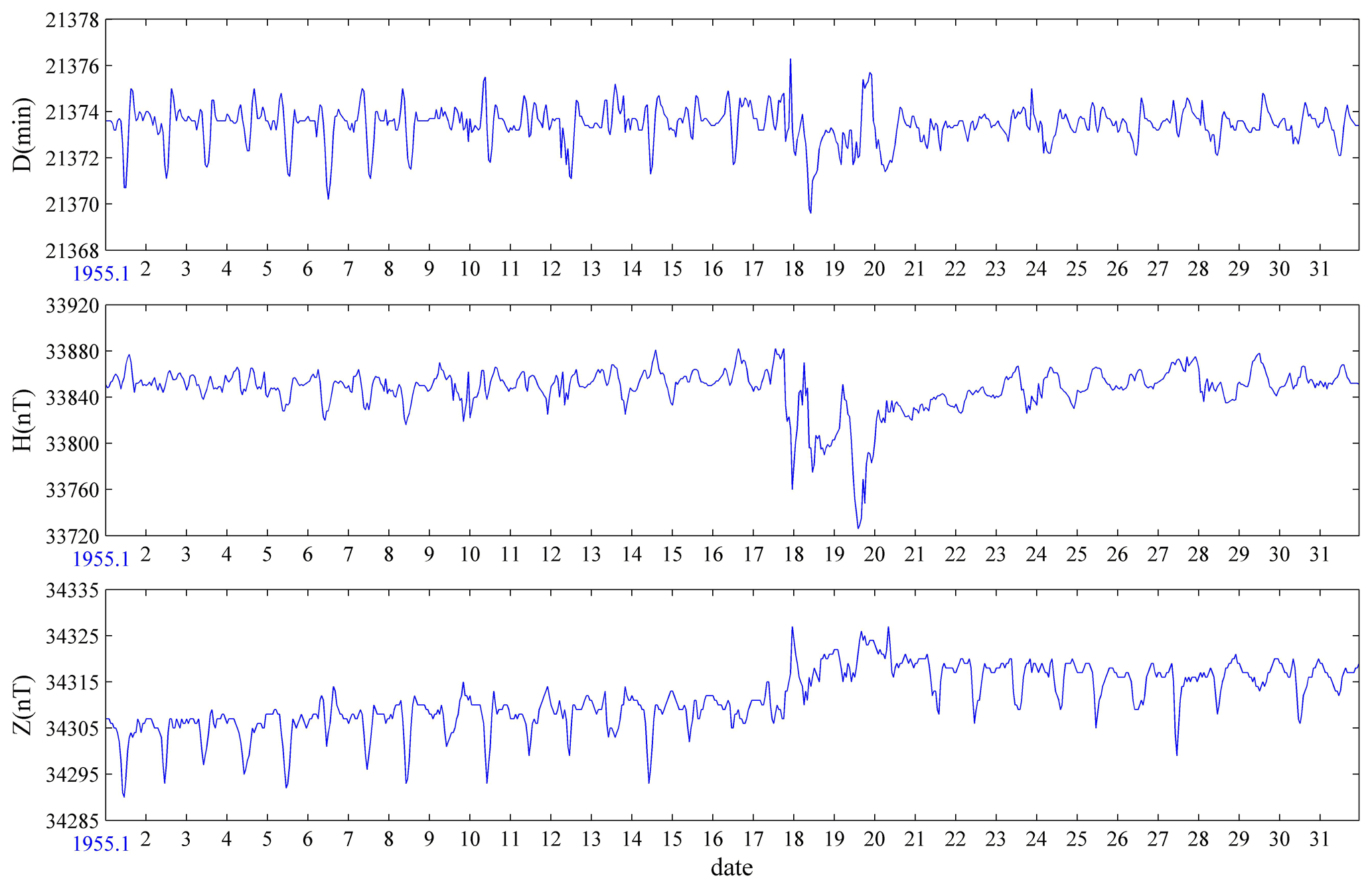
   We checked the AHMV plots of the SSH month by month and found that sometimes the geomagnetic changes were quiet and regular, sometimes violent and irregular, and most of the days the geomagnetic changes were superimposed on the regular quiet day changes with some disturbances of different shapes and amplitude. As shown in Fig. 6, taking the AHMV record of January 1955 as an example, it can be seen from the figure that the record includes both regular periodic quiet day changes and complex perturbation, and the geomagnetic storms of 18–19 January are violent disturbances.

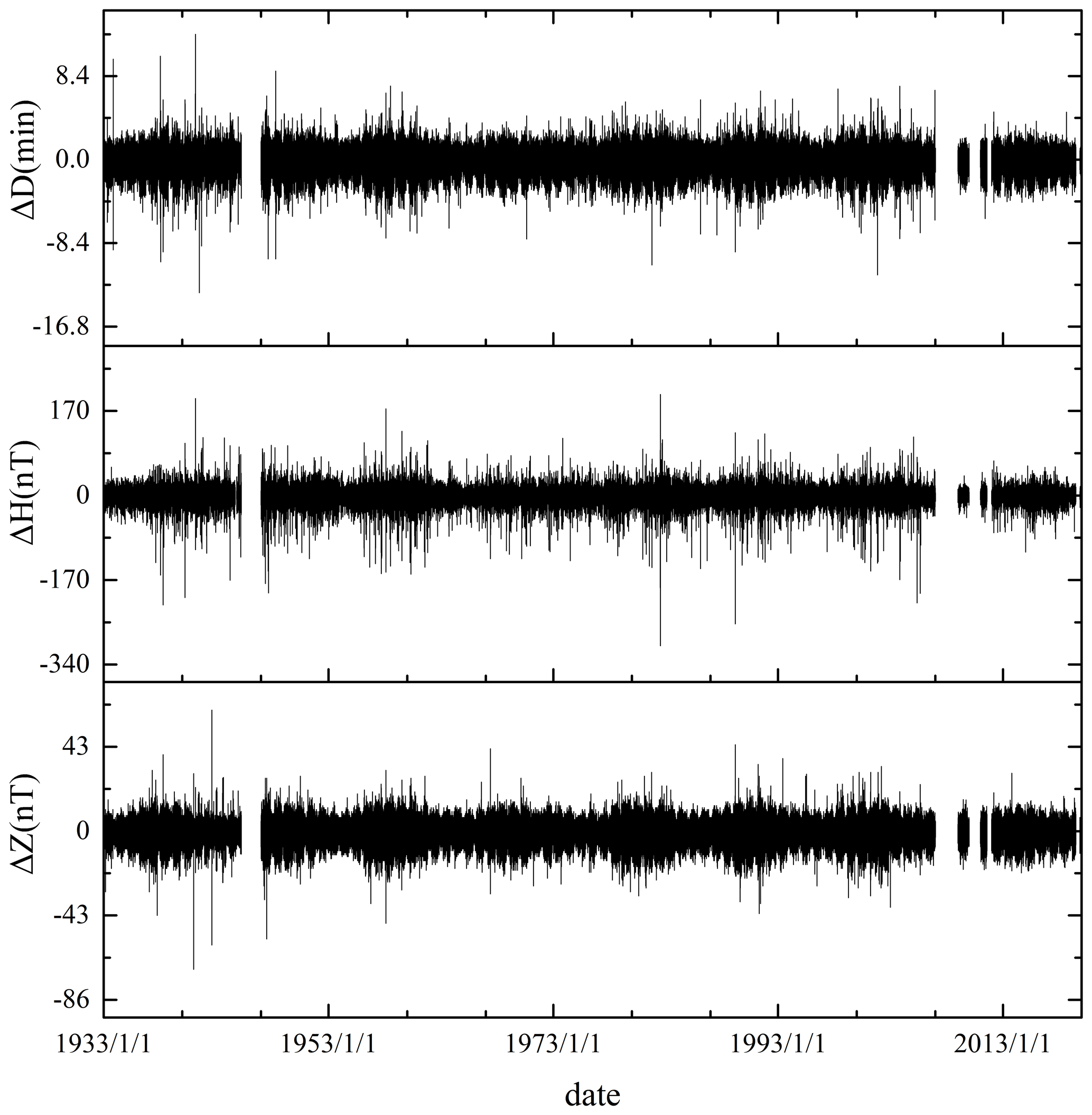
   In order to eliminate the impact of trend and detect the data problems more effectively, we plotted the first-time derivative (FTD) of AHMVs for D, H, and Z components (Fig. 7). We calculated the FTD using the consecutive values of hourly series (Morozova et al., 2014). For all geomagnetic components, the FTD is calculated as

   $$\begin{array}{}\text{(2)}& \mathrm{d}X/\mathrm{d}t\left(\mathrm{hour}\right)=\left(X\right(\mathrm{hour})-X(\mathrm{hour}-\mathrm{1}\left)\right)/\mathrm{1},\end{array}$$

   where X denotes the geomagnetic field components D, H, and Z.

   The FTD plots are also particularly useful in evaluating artificial noise, especially interference in the shape of steps or spikes (Linthe et al., 2013; Pang et al., 2013; Chen et al., 2014). It can be seen from the figure that the data after the FTD eliminates the trend change, and the data are steady, going up and down within a certain range; ΔD varies between −13.4 and 12.6 min, ΔH varies between −302 and 203 nT, and ΔZ varies between −70 and 62 nT.

3. The tolerance test detects the outliers and compare with geomagnetic indices.

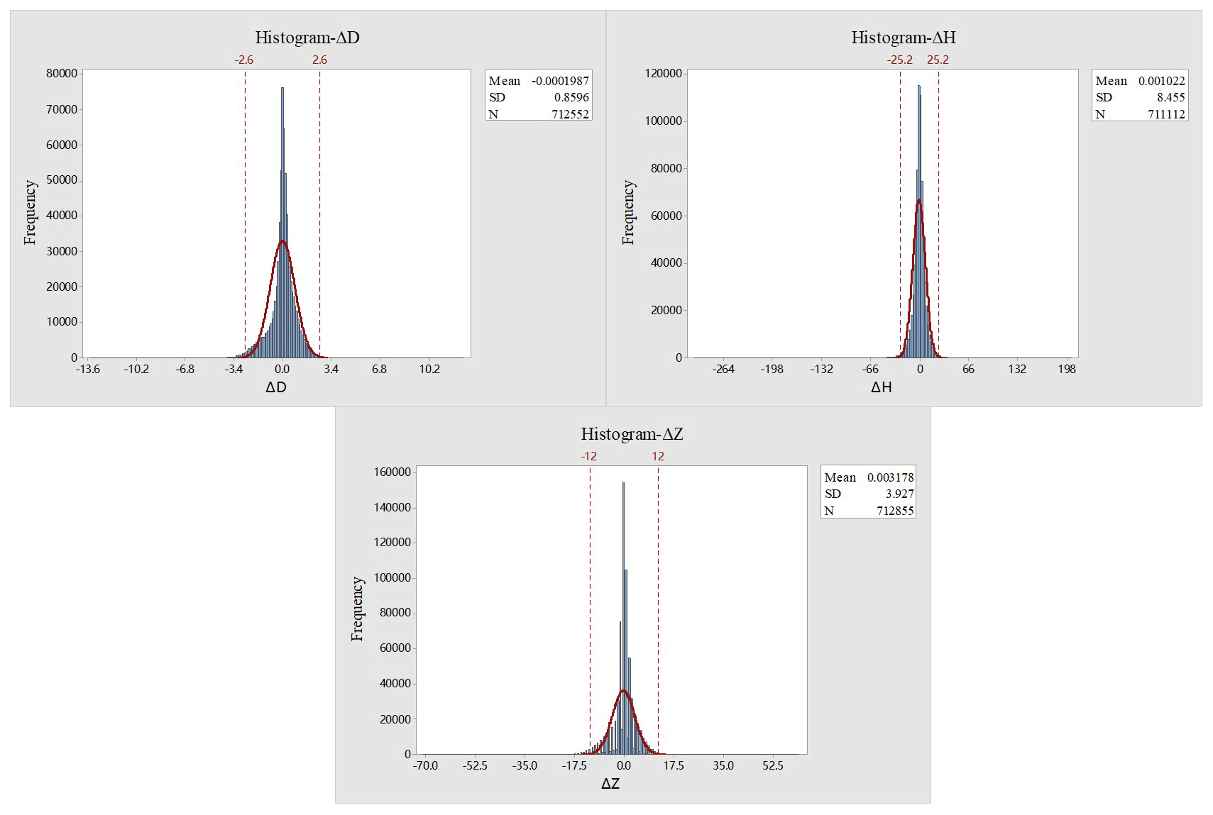
   For a large set of data with a normal or approximately normal distribution, 99.7 % of the values are distributed in the (μ−3σ, μ+3σ) interval, where σ and μ are the standard deviation and mean for all time, respectively. The values beyond this interval are generally considered as outliers. We presented the histograms of the FTD of D, H, and Z components between 1933 and 2019 in Fig. 8, which aimed at detecting the outliers further. The distribution can be well modeled by the Gaussian probability density function (solid red curve). The vertical dashed red lines indicate the lower and upper limits obtained by applying the criteria (μ−3σ) and (μ+3σ). We found that more than 98.6 % of the FTD data points fall within the range of 3 times the standard deviations.

Figure 5 The AHMV plots of D, H, and Z components for all time from 1933 to 2019.

Figure 6 The AHMV record of January 1955 at SSH.

Figure 7 The FTD plots of D, H, and Z components.

Figure 8 The histogram of the FTD of between 1933 and 2019.

For the FTD data exceeding 3 times the standard deviation, we defined them as FTD outliers. We need to confirm whether the outlier is related to geomagnetic activity. Two conventional indices to describe geomagnetic activity are Kp and Dst; Kp has no linear relationship with the geomagnetic activity, so the ap index was introduced. The ap is expressed in “ap units”: 1 ap unit equals 2 nT (Menvielle et al., 2011). Currently, Kp and ap indices are produced by the GeoForschung Zentrum (GFZ) Potsdam, Germany (Kp and ap values since 1932 are available online at https://www.gfz-potsdam.de/, last access: 18 November 2022, GeoForschung Zentrum Potsdam Website, 2022); Dst indices are currently produced by the World Data Center for Geomagnetism, Kyoto (Dst values since 1957 are available online at http://wdc.kugi.kyoto-u.ac.jp/, last access: 18 November 2022, World Data Center for Geomagnetism, Kyoto, 2022). The comparative analysis (Fig. 9) also shows that the geomagnetic components have a good correlation with Dst and ap indices, especially H and Dst. It should be noted that the H component in Fig. 9 has eliminated periodic changes such as secular variation and seasonal variation.

Figure 9 Comparative analysis of the H components with Dst and ap indices.

We compared the FTD outliers with the ap and Dst indices trying to establish the cause of the FTD out of tolerance, and took corresponding measures: (a) When the ap is greater than or equal to 24 nT, or Dst is less −30 nT, the outlier was considered to be caused by geomagnetic activity. The AHMVs at the corresponding time were not corrected. (b) When the ap is less than 24 nT and Dst is greater than −30 nT, we carefully looked for the cause of each FTD outlier by comparing the daily variation curves of multiple observatories (Sheshan, Chongming, Wuhan, Guangzhou, or Nanjing), and further consult the available documentation (Observatory Communication Journal, Geomagnetic Observation Report, Chronicles of China Geomagnetic Observatory, and postal letters). A preliminary analysis found that for the D component, 65.6 % of the outliers were related to geomagnetic disturbance; the 33.5 % showed that no abnormality was found in the daily change curve; the remaining 82 values were questionable. For the H component, 80.5 % of the outliers were related to geomagnetic disturbance; the 17.6 % showed that no abnormality was found in the daily change curve; the remaining 199 values were questionable. For the Z component, 99.6 % of the outliers were related to geomagnetic disturbance; the 0.4 % showed that no abnormality was found in the daily change curve; the remaining 112 values were questionable. A total of 393 FTD outliers were questionable and no relevant and useful information was recorded in the available documentation. The AHMVs at the corresponding time were not corrected but were marked as questionable data in the datasets, the quality flag was QC = Q. As shown in Fig. 10, taking the FTD outliers of 19 October 2013 as an example, a clear deviation was found in the data between 08:00 to 13:00 from the real geomagnetic characteristics. Due to the lack of complete documentation, the questionable data were not corrected, just made the marks in the datasets, QC = Q. (c) When the ap index is less than 24 nT and Dst is greater than −30 nT, a change is registered in the available documentation. These data can be accepted to be corrected. In Table 2, we listed the date of the data to be corrected and the reasons recorded in the daily log and annual report. It took place only on 1 January 2003, a modern absolute instrument named Fluxgate Theodolite DIM-100 replaced the geomagnetic induction instrument Schulze, and an Overhauser Effect Proton Precession Magnetometer GSM-19F replaced the Proton Precession Magnetometer CZM-2. These changes led to sudden steps in size of about 1.9^′, 8, 40, and 35 nT in D, H, Z, and F components, respectively. The log recorded the exact jumps in the measurements during the change of instruments at that time (SSH observatory, 2004).

Figure 10 The contrast curve of SSH, COM, WHN, and GZH from 15 to 24 October 2013.

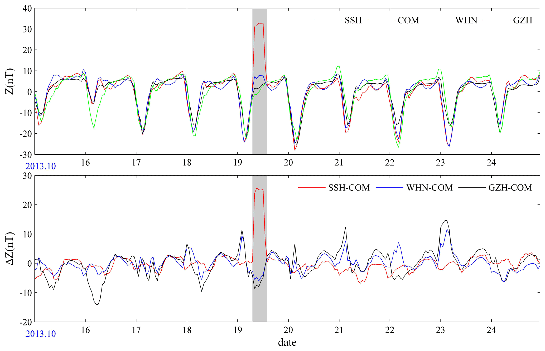
Table 2 Date and the reasons recorded of the data to be corrected.

4 Correction of the data problems

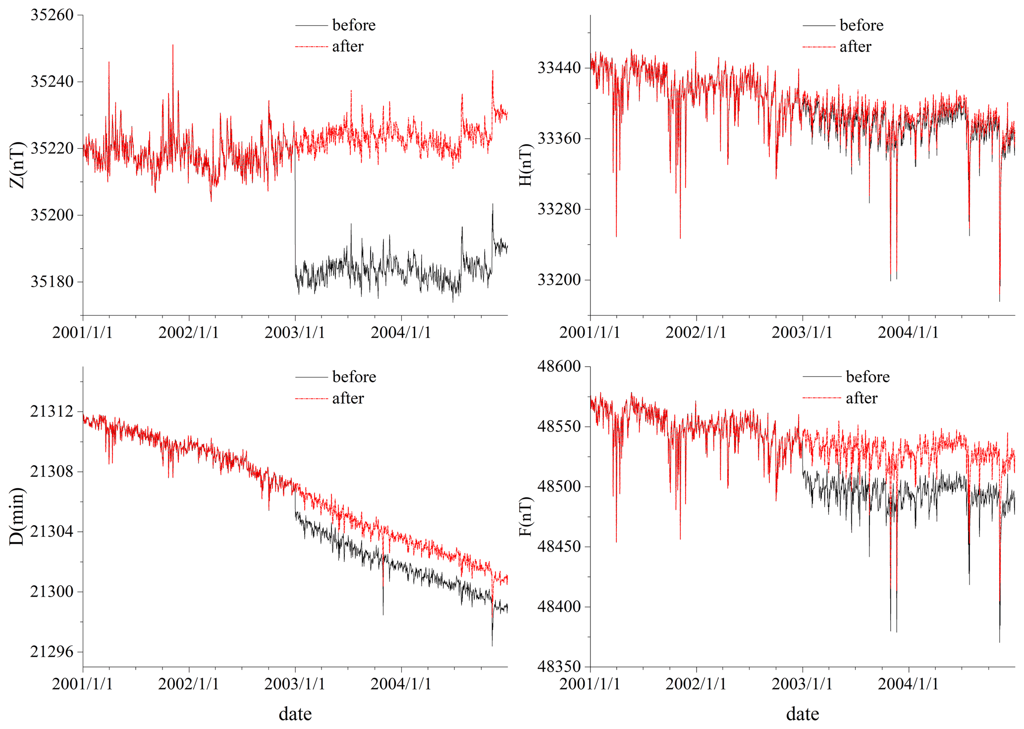
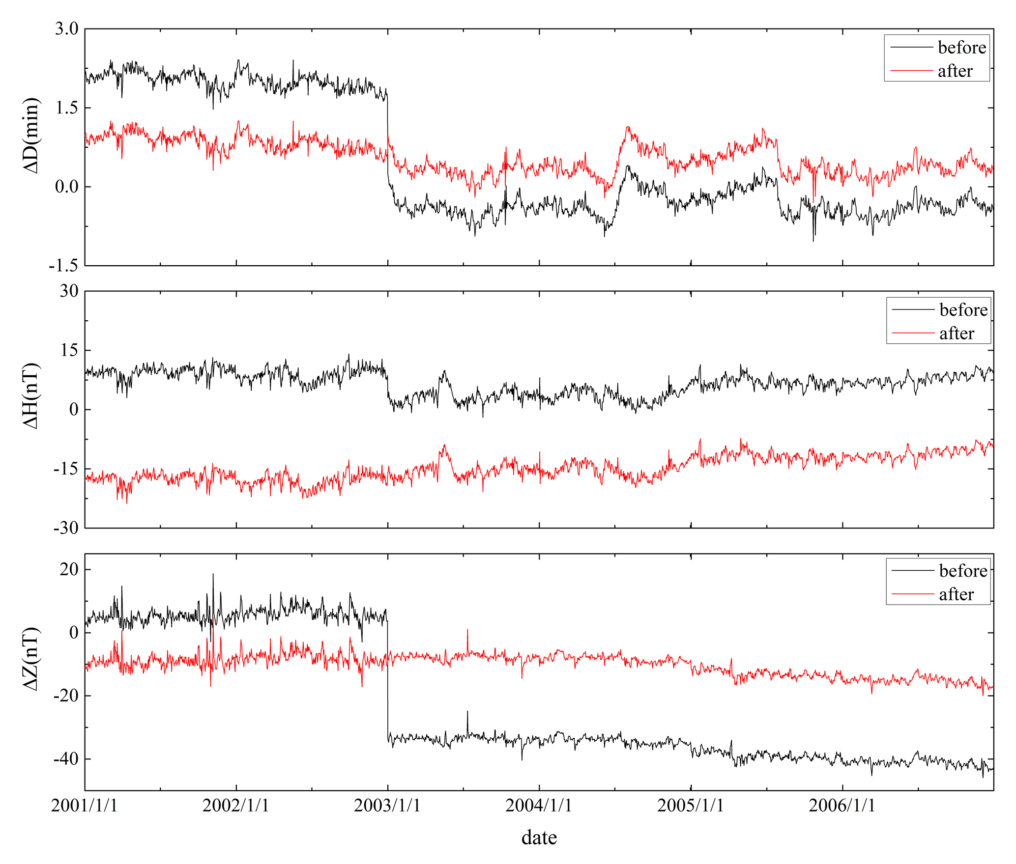
As was mentioned above, we only corrected the data of D, H, Z, and F components that occurred after 1 January 2003. The break arose due to the installation of new instruments in 1 January 2003. The corrected value is 1.9^′ for the D component, 8 nT for the H component, 40 nT for the Z component, and 35 nT for F component (see Table 2). As shown in Figs. 11 and 12, we gave the hourly and daily mean values curve of the D, H, and Z components before and after correction from 1 January 2001 to 31 December 2004. It can be seen that the quality of data has been greatly improved after correction.

The curve of the AHMVs shows obvious annual and seasonal variations. The seasonal variation shows that the variation range is large in summer and small in winter. The absolute daily mean value (ADMV) curve of the D component shows an obvious long-term trend of slow decline from 2001 to 2004. No obvious change characteristics can be seen in the Z curve.

Figure 11 Plot of hourly mean values before and after correction.

Figure 12 Plot of daily mean values before and after correction.

Mutual comparison is an important method to check data quality. In general, the difference of the same component between two stations close to each other is small and stable. We also compared the data of the SSH before and after correction with those data from the Chongming Geomagnetic Observatory (IAGA code COM), which is the nearest observatory from the SSH (Fig. 13). The differences of the three components before correction are as follows: ΔD varies between −1.0 and 2.4 min, ΔH varies between −2 and 14 nT, and ΔZ varies between −46 and 19 nT. The differences of the three components after correction are as follows: ΔD varies between −0.3 and 1.3 min, ΔH varies between −7 and 24 nT, and ΔZ varies between −20 and 4 nT. The standard deviations of the differences of the three components before correction are as follows: 1.1 min, 3 nT, and 20 nT. The standard deviations of the differences of the three components after correction are as follows: 0.3 min, 3 nT and 3.3 nT. Again, it shows that the quality of observation data is improved after correction.

Figure 13 Plot of difference between the SSH and COM before and after correction.

5 Validation of the corrected series by compare with reference series

Intercomparison of time series for geomagnetic elements from adjacent observatories or geomagnetic models is also an important method to test accuracy and stability of data (Curto and Marsal., 2007). Firstly, we compared the rescued data with those data from the reference observatory. In China, the regular observation of most geomagnetic observatories began in the 1980s. Only eight geomagnetic observatories were established during the international geophysical year (Rasson et al., 2011). Among the eight observatories, the Guangzhou observatory (GZH) is closer to the Sheshan observatory. It started observation early, and the quality of observation data was good. So, we selected the GZH as the reference observatory. The GZH is located in Guangzhou City, Guangdong Province, about 1240 km northeast of the SSH. It began geomagnetic observation in 1957. Due to the interference of Guangzhou metro operation, the new site, Gaoyao Liantang Town, was selected in 1996. The construction of the new observatory was completed at the end of 2001. The geomagnetic observation records officially began in the new place on 1 January 2002.

We used GDPST which offers very useful diagnostic procedures of the data quality to plot intercomparison of the value curve and their difference curve from the SSH and GZH observatories on hourly and daily timescales to detect data with potential quality issues year by year. As an example, we presented AHMVs, ADMVs and their difference curves of the SSH and COM observatories in Fig. 14. At Fig. 14 in the upper panel (a), the AHMV and their difference curves are depicted, while in the lower panel (b), the ADMVs and their difference curves are plotted. On hourly scales, the single components D, H, and Z of the SSH and GZH behave roughly identical, and their difference series slowly fluctuates (due to geomagnetic activity) around a certain range. Spikes are caused in most cases by external disturbances. On daily timescales, the components D, H, and Z are roughly identical, but their differences clearly coincide with the variation of the geomagnetic field. It is because the distance between the two observatories are too far to completely offset the influence of internal and external source fields in different regions.

Figure 14 AHMVs, ADMVs and their difference curves of the SSH and GZH observatories. (a) AHMVs and their difference curves. (b) ADMVs and their difference curves.

Comparing the measured values with the calculated values of the model for a long-time scale is not only an important means to check the stability of secular variation, but also an important means to evaluate the accuracy of the model (Zhang et al., 2008b; Chen et al., 2012). One of the aims of geomagnetic observatories is the monitoring of SV (Reda et al., 2011). Secondly, to monitor the SV of SSH, we compared the series curve of the annual mean values (AMVs) for the X, Y, and Z components calculated from the rescued records with these data calculated from the COV-OBS model (Gillet et al., 2013; Huder et al., 2020). The COV-OBS.x2 model covers the period from 1840 to 2020. The data source of the model is from observatory data, satellite data, and the older surveys. The model can give the field contributions from the internal and external sources.

As can be seen from the Fig. 15, the change trends of X, Y, and Z components from the SSH and COV-OBS model are very consistent. The X component increased year by year before 1962 and generally decreased after 1962; from 1933 to 2019, the Y component shows a general downward trend and the Z component shows a general upward trend. There are differences between AMVs of the SSH and these data calculated from the COV-OBS model, the X component varies from −210 to −276 nT, the Y component varies from 17 to 94 nT, and the Z component varies from 198 to 289 nT. According to the preliminary analysis, the main reasons for the large difference between the SSH and COV-OBS model may be the local magnetic anomaly in the Sheshan area, the uneven distribution of global stations, the lack of modeling data, and data-quality problems in the SSH. This fully illustrates the importance of continuous and high-quality data in magnetic field modeling.

Figure 15 The AMV and their difference curves of X, Y, Z components calculated from the rescued records and the COV-OBS model.

Figure 16 The SV of the annual Y series from the SSH and COV-OBS model.

6 Application examples of SSH datasets

We calculated the first-time derivative (FTD) using a difference between 2 consecutive years as SV and plotted the SV from the rescued data and COV-OBS model to detect possible geomagnetic jerks over the past 90 years. For all geomagnetic components, the SV is calculated as

$$\begin{array}{}\text{(3)}& \mathrm{d}X/\mathrm{d}t\left(\mathrm{year}\right)=\left(X\right(\mathrm{year})-X(\mathrm{year}-\mathrm{1}\left)\right)/\mathrm{1},\end{array}$$

where X denotes the geomagnetic field components D, H, and Z.

Table 3 List of geomagnetic storms that have occurred at the SSH since 1933.

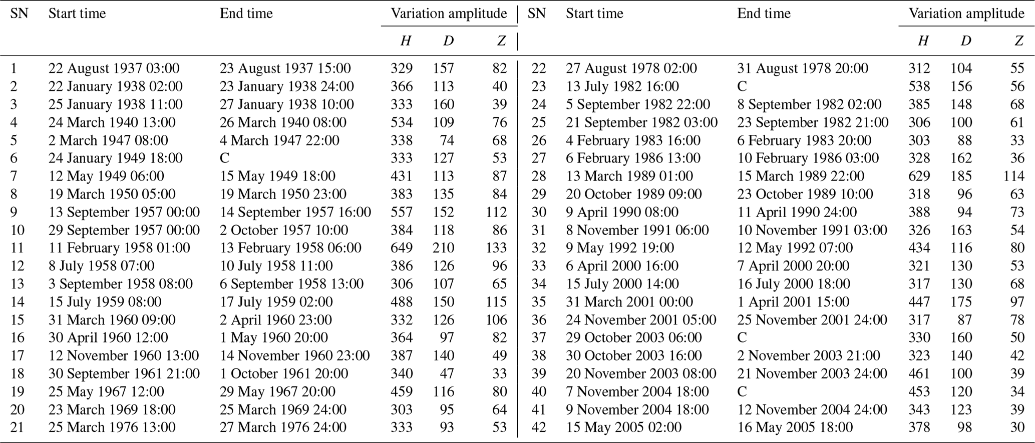
Note C in “End time”: followed by another storm.

Figure 17 The geomagnetic storm occurred on 11 February 1958.

Geomagnetic jerks are defined as V-like or Λ-like changes in the SV and occur in a time period of a few months (Courtillot and Le Mouël, 1984; Morozova et al., 2014; Kang et al., 2020). “The geomagnetic jerks are due to interactions of the core field and the rapid time-varying core flow” (Kuang and Tangborn, 2011). Since Malin and Hodder (1982), Courtillot and Le Mouël (1984) discovered the geomagnetic jerk in 1969, 10 jerks have been detected in observatories from 1933 to 2020, of which 1969, 1978 (Alexandrescu et al., 1996), 1991 (De Michelis et al., 1998), 1999 (Mandea et al., 2000; Zhang et al., 2008a), 2003 (Mandea and Olsen, 2007; Feng et al., 2018; He et al., 2019), 2007 (Kotzé, 2010; Chulliat et al., 2010), and 2014 (Brown et al., 2016; Kloss and Finlay, 2019; Finlay et al., 2016; Kang et al., 2020) were global events. In addition, there were two local events which occurred in 1949 (Mandea et al., 2000) and 2011 (Chulliat and Maus, 2014; Kotzé and Korte, 2016). In 2017, there were similar characteristics of geomagnetic jerks, which may be a new geomagnetic jerk (He et al., 2019; Pavón-Carrasco et al., 2021). The jerks are more easily seen in the eastward component (Y) of the geomagnetic secular variation. Not all jerks can be detected around the world, some seem to be seen only in limited regions (Morozova et al., 2014), and its occurrence time is not exactly the same at each observatory.

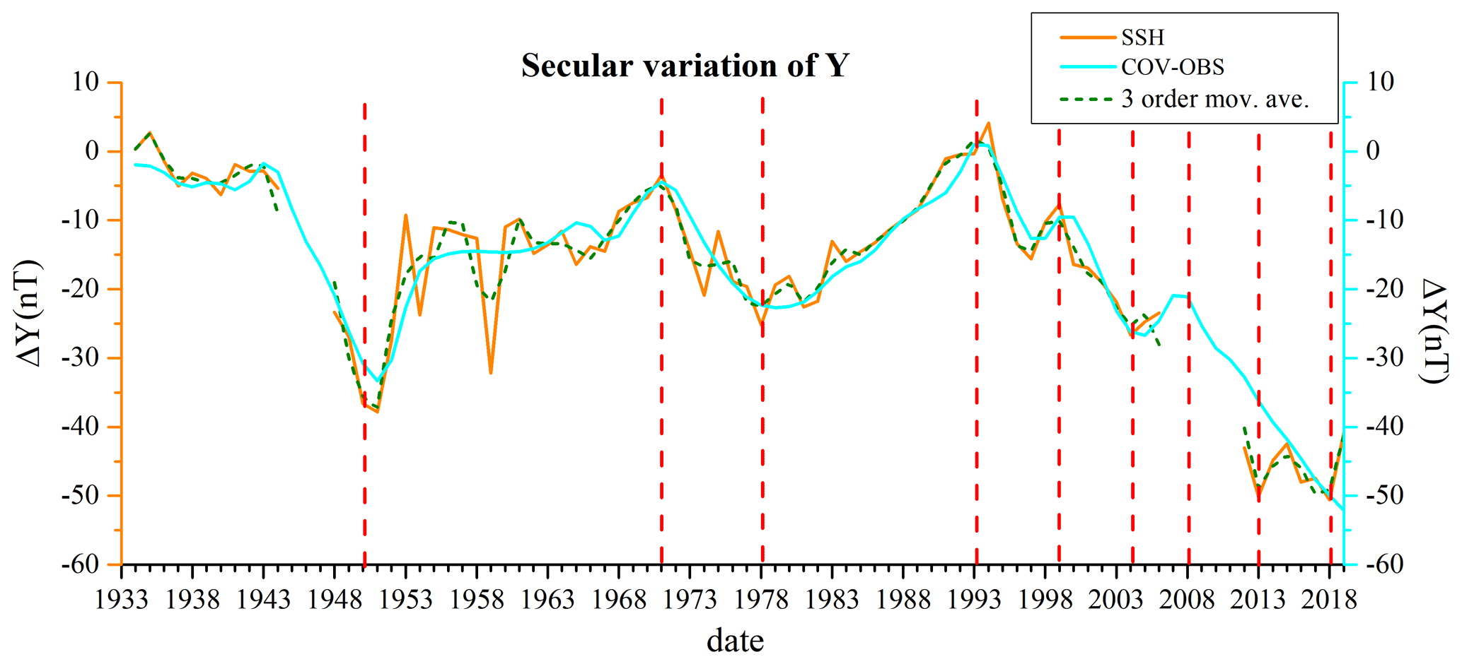
Figure 16 gives the SV of the annual Y series from the SSH and COV-OBS model, and the dotted blue line is the third-order moving average curve of the Y component SV at the SSH. Nine jerks are clearly seen in the plot. They occurred in 1950, 1971, 1978, 1993, 1999, 2004, 2008, 2013, and 2018. Except for the jerks that occurred in 1978 and 1999, other events were a little later as seen at the SSH. Between 2008 and 2017, only one jerk (in 2013) is seen at the SSH, which is inconsistent with the study of other scholars mentioned above. They observed jerk events in 2011 and 2014, respectively. We cannot see a potential jerk in 2011, maybe because of the data gap until 2011.

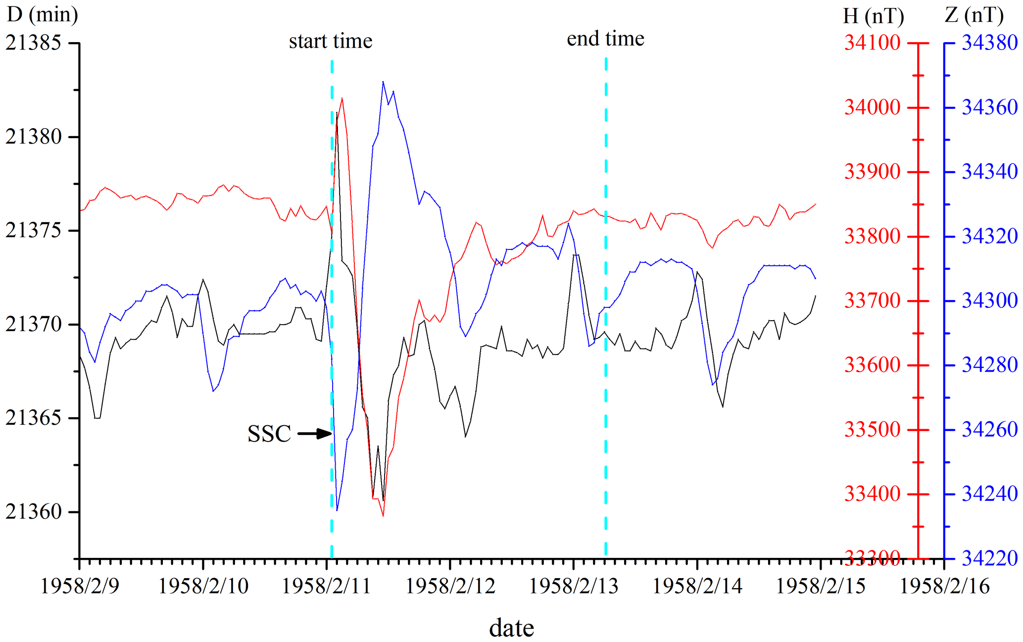
A geomagnetic storm is a global phenomenon of magnetic disturbance. At low and mid-latitudes, it mainly manifests itself as a decrease in the horizontal geomagnetic field (H) during a geomagnetic storm. According to the Kakioka Magnetic Observatory Website (2022), a total of 67 very large geomagnetic storms (variation range of the H component >300 nT) have occurred since 1933. Referring to the start and end time of the geomagnetic storm announced by the website, we studied the geomagnetic storms that were recorded in the data series of the SSH since 1933. We found a total of 42 very large geomagnetic storms (variation range of the H component >300 nT) in these data series (Table 3). Figure 17 shows an example of a very large geomagnetic storm that occurred on 11 February 1958. A sudden storm commencement (SSC) occurred at 01:00 on 11 February 1958. It is the sign of the start of the geomagnetic storm. This storm lasted about 53 h and ended at 06:00 on the 13 February 1958. The maximum variation amplitude of D, H and Z during the geomagnetic storm is 210, 649 and 133 nT respectively.

7 Data availability

The digitized and quality-controlled absolute hourly mean value (AHMV) data are available at: https://doi.org/10.5281/zenodo.7005471 (Zhang et al., 2022). The data are provided in Microsoft Excel format, including the observed AHMV files of the three components (D, H and Z) at the SSH for 1933–2019, and also the metadata files about the datasets.

8 Conclusion

This paper presents the acquisition process, quality control, data correction, quality examination, and application examples of the datasets of the SSH from 1933 to 2019. The quality examination results show that the corrected data have a good agreement with the reference observatory data and the model data. This fully indicates that the rescued data are of good quality. The datasets are valuable for studying the geomagnetic daily variation, geomagnetic field model construction, and secular variation. It should be noted that the data marked with Q (QC = Q) are used with caution for the reasons mentioned above. A few problems were found in the acquisition of geomagnetic historical datasets: (1) the rescue of paper data is a time-consuming and laborious work. For example, the font color of some reports is light, which makes automatic recognition difficult. We can only recognize and input by key. (2) Some metadata of the SSH has been missing, which brings difficulties to the identification and correction of data. Therefore, we believe that we should do our best to rescue historical data to avoid the irreparable losses over time. Our plan for the next phase is to rescue the historical data from 1874 to 1932 at SSH, as well as from other observatories, to provide more high-quality data for the geomagnetic science community.