Colombian soil texture: building a spatial ensemble model

Texture is a fundamental soil property for multiple applications in environmental and earth sciences. Knowing its spatial distribution allows a better understanding of the response of soil conditions to changes in the environment, such as land use. This paper describes the technical development of Colombia's first texture maps, obtained via a spatial ensemble of national and global digital soil mapping products. This work compiles a new database with 4203 soil profiles, which were harmonized at five standard depths (0–5, 5–15, 15–30, 30–60, and 60–100 cm) and standardized with additive log ratio (ALR) transformation. A compilation of 83 covariates was developed and harmonized at 1 km² of spatial resolution. Ensemble machine learning (EML) algorithms (MACHISPLIN and landmap) were trained to predict the distribution of soil particle size fractions (PSFs) (clay, sand, and silt), and a comparison with SoilGrids (SG) products was performed. Finally, a spatial ensemble function was created to identify the smallest prediction errors between EML and SG. Our results are the first effort to build a national texture map (clay, sand, and silt fractions) based on digital soil mapping in Colombia. The results of EML algorithms showed that their accuracies were very similar at each standard depth, and were more accurate than SG. The largest improvement with the spatial ensemble was found at the first layer (0–5 cm). EML predictions were frequently selected for each PSF and depth in the total area; however, SG predictions were better when increasing soil depth in some specific regions. The final error distribution in the study area showed that sand presented higher absolute error values than clay and silt fractions, specifically in eastern Colombia. The spatial distribution of soil texture in Colombia is a potential tool to provide information for water-related applications, ecosystem services, and agricultural and crop modeling. However, future efforts need to improve aspects such as treating abrupt changes in the texture between depths and unbalanced data. Our results and the compiled database (https://doi.org/10.6073/pasta/3f91778c2f6ad46c3cc70b61f02532db, Varón-Ramírez and Araujo-Carrillo, 2022, https://doi.org/10.6073/pasta/d6c0bf5847aa40836b42dcc3e0ea874e, Varón-Ramírez et al., 2022) provide new insights to solve some of the aforementioned issues.

1 Introduction

Soil texture is defined by the proportion of particle size fractions (PSFs), called clay, silt, and sand (Richer-de Forges et al., 2022). Soil texture is important to understand soil processes related to agriculture and the environment from the field to the continental scale (Radočaj et al., 2020; Malone et al., 2021; Bönecke et al., 2021; Caubet et al., 2019). For example, soil texture is a fundamental soil property for characterizing soil productivity and soil fertility (Patel et al., 2021; Soropa et al., 2021). Soil texture plays a fundamental role in quantifying the capacity of soils to store carbon and retain the water required for plants to grow (Dharumarajan and Hegde, 2020; Zhang and Hartemink, 2021). Additionally, the soil texture study must include two principal statements: first, it is compositional data, which means that PSF sum to 100 % (%clay+%sand+%silt), and this statement must be satisfied at each location (Amirian-Chakan et al., 2019); second, the proportion of PSF could variate between horizons depending on soil forming factors interactions (Orton et al., 2016; Poggio and Gimona, 2017).

Spatial predictions of soil properties (e.g., particle size fractions proportion) or classes (e.g., soil textural class) across areas where no soil data exist is the primary motivation of digital soil mapping (or pedometric mapping) (McBratney et al., 2003). In digital soil mapping (DSM), soil properties (continuous or categorical) for a specific soil depth and a given location in the geographical space can be predicted as a function (e.g., empirical function) of the soil forming environment (climate, organisms, topography, geology, ecology, atmosphere, and human interventions to soils) (Grunwald et al., 2011). These environmental prediction factors are commonly acquired from four primary sources: remote sensing, digital terrain analysis, climate, and thematic maps (e.g., soil type, rock type). The use of prediction algorithms or models that can account for the spatial variability of soil distribution is the basis of DSM (Wadoux et al., 2021a; Khaledian and Miller, 2020).

Predictions of quantitative soil properties (e.g., percentages of clay, silt, and sand) (Liu et al., 2020; Li et al., 2020) or the probability of presence/absence of a soil class (e.g., a soil textural class) (Ramcharan et al., 2018; Kaya and Başayiğit, 2022) are represented on digital soil maps for a given soil depth and a specific period. These predictions or probability estimates are derived from the use of supervised statistical learning (in the presence of training data for a response variable) or unsupervised statistical learning (in the absence of a response variable) (James et al., 2013). Statistical learning methods for supervised learning (e.g., for upscaling soil texture data using digital elevation models) can be applied to categorical (e.g., to solve classification problems) or numerical (to solve prediction problems) datasets (Bischl et al., 2016). There are hundreds (if not thousands) of modeling approaches for solving regression and classification problems. We could classify these methods into two modeling cultures: one assumes that a given stochastic data model generates the data, and the another uses algorithmic models and treats the data mechanism as unknown (Breiman, 2001). However, it is not easy to classify the immense diversity of modeling approaches and their possible combinations. Therefore, the problem of model or algorithm selection to perform predictions in DSM is an emergent research question.

Geostatistics and machine learning are the two principal forms of statistical learning in DSM (Hengl and MacMillan, 2019). Geostatistics is a branch of statistics that deals with the values associated with spatial or spatial–temporal datasets (Webster and Oliver, 2007). In contrast, machine learning is a computer-assisted branch of statistics that uses algorithms developed to solve prediction problems (Witten et al., 2011). Machine learning models are commonly parameterized (selection of multiple modeling parameters) using multiple resampling techniques, such as cross-validation or bootstrapping (Brenning, 2012). These resampling techniques allow the algorithm to “learn” from the data using the capacity of computers to store results from multiple data configurations following the same statistical treatment. This computer-assisted learning allows machine learning algorithms to reproduce the relationship between the response and the prediction factors in the statistical space and can be applied to soil datasets to generate digital soil maps. Machine learning algorithms can be roughly divided into four main groups: (a) conventional machine learning based on trees, kernels, linear based, or probabilistic algorithms; (b) reinforcement learning algorithms; (c) deep learning algorithms; and (d) ensemble learning algorithms. The last extracts information from multiple modeling approaches and combines them to create a better solution for a given prediction problem (Yang, 2017).

Recent developments in ensemble learning efforts have demonstrated great potential for improving the accuracy and spatial detail of current estimates of soil functional properties across scales (Hengl et al., 2021; Wadoux et al., 2020; Llamas et al., 2020). Several experiences with the mapping of soil texture at different depths have been done: France (Mulder et al., 2016), Scotland (Poggio and Gimona, 2017), Hungary (Laborczi et al., 2019), or China (Liu et al., 2020) are some examples. However, few of them have used spatial ensemble techniques. One representative case was developed by Hengl et al. (2021) for the continent of Africa at three depths (0, 20, and 50 cm) and 30 m spatial resolution. They produced predictions using two scale 3D ensemble machine learning (EML) framework and 122 200 training samples (approximately); their study utilized an improved predictive mapping framework: spatially-adjusted EML, that better accounts for spatial clustering of points. The spatial cross-validation methodology was a special point of their work, obtaining RMSE values of 9.6 %, 13.7 %, and 8.9 % for clay, sand, and silt, respectively. Their results proved to be more accurate than previous works, which was attributable to the addition of higher resolution remote sensing images and digital terrain parameters (DTMs), the adoption of methodological improvements in hyper-parameter tuning, selection of features, and implementation of ensemble models (Hengl et al., 2021).

Colombia has produced maps, either PSF or textural classes, at a national scale through conventional mapping and regional scale using DSM. On a national scale, these maps use a series of delineations based on qualitative soil characteristics, called cartographic soil units (CSUs). These studies have been produced in different periods: Cortés et al. (1982) (scale 1:5 000 000), IGAC (2003) (scale 1:500 000), and IGAC (2015) (scale 1:500 000). The map carried out by IGAC (2015) represented the PSF through four textural groups of soils (very fine, fine, medium, and coarse) in a layer from 0 to 50 cm; however, this methodology ignores the spatial variability inside the CSU. On a regional scale, Araujo-Carrillo et al. (2021) used machine learning algorithms to show the spatial distribution of clay (%) and its prediction error. However, they ignore the statement of compositional data of the soil texture, and their study just included the surface layer of the soil (0–20 cm).

In this work, first, we compared and tested two ensemble machine learning approaches applied to predict soil texture at national scales in Colombia. Second, we compared our results with the global product SoilGrids (SG). Third, we built an ensemble map developing a pixel-wise solution to identify the method with lower prediction error. We hypothesized that multiple prediction algorithms could capture the spatial variability of soil texture differently because they treat the data in different ways to solve prediction problems (e.g., using decision boundaries or probability thresholds or hypothesis of the empirical relationship between the response and the prediction factors). Understanding which prediction algorithms and approaches yield lower error levels at the pixel level could benefit model selection efforts in DSM.

2 Methodology

Our workflow contains five significant steps: harmonization and transformation of soil data, selection of covariates, spatial prediction with different algorithms, validation, and spatial ensemble. These sections will be discussed in detail below.

2.1 Dataset

A total of 4203 georeferenced (EPSG:4326) soil profiles were collected from Sistema de Información de Suelos de Latinoamérica y el Caribe – SISLAC, a soil information system developed by FAO (FAO, 2020), that all contained information about soil PSF. These PSF are classified according to the United States Department of Agriculture (USDA) system: clay (particles smaller than 0.002 mm in diameter), silt (particles sizes from 0.002 to 0.05 mm in diameter), and sand (particles sizes from 0.05 to 2.00 mm in diameter). The soil data covered five natural regions (geographic division made based on climatic, vegetation, relief, and soil class conditions) and 31 districts of the continental area of Colombia (Fig. 1) (Rangel-Ch and Aguilar, 1995). The regions were Caribbean in the north, Pacific in the west, Andean in the center (corresponding to the Andes Mountains), Orinoquia in the east, and Amazon in the south.

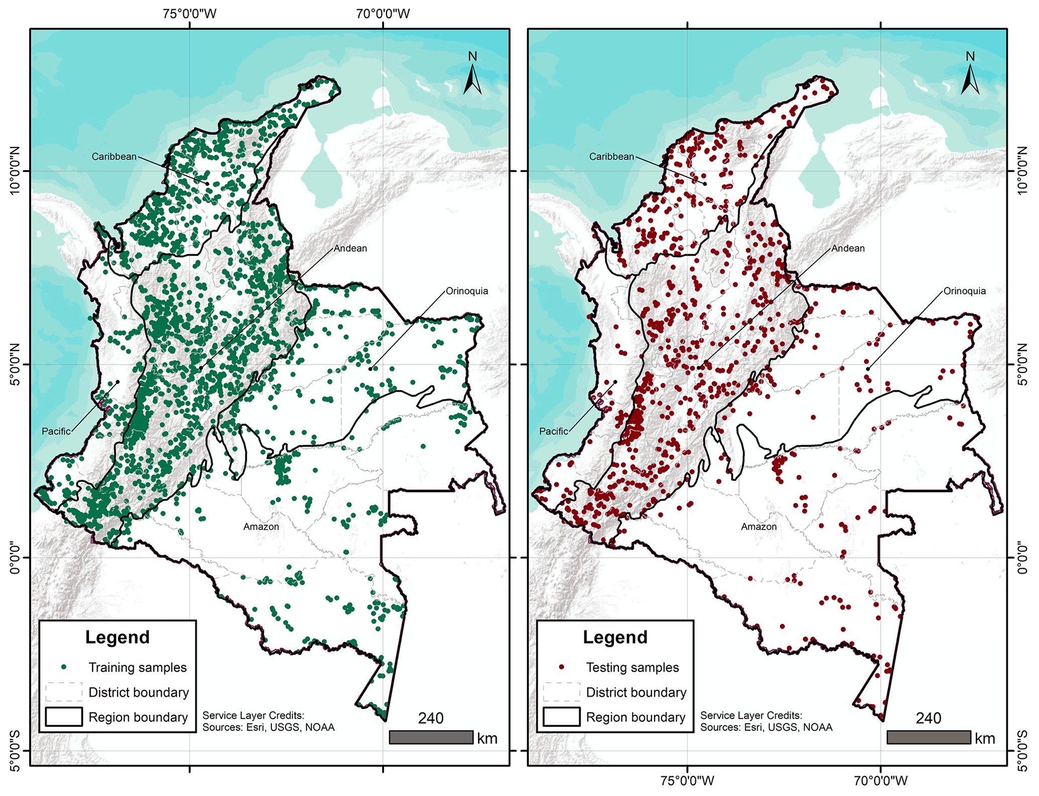
Figure 1 Soil sample points distribution at 0–5 cm depth (left: training samples, right: testing samples).

2.2 Data harmonization and transformation

Dataset quality was ensured by (i) sum of PSF equals 100 % and (ii) no overlapping sampling depth. PSF were harmonized to five standard depths (0–5, 5–15, 15–30, 30–60, and 60–100 cm), following the vertical discretization in the GlobalSoilMap specifications (Arrouays et al., 2014). The distribution of soil profiles by depth was 4203 at 0–5 cm, 4201 at 5–15 cm, 4153 at 15–30 cm, 3974 at 30–60 cm, and 3597 at 60–100 cm. The soil information for each depth was obtained using a quadratic function of depth with equal areas (spline) (Bishop et al., 1999), through the mpspline function of the aqp package (Beaudette et al., 2013) of R version 4.0.3.

A D-part composition is an element where all its components are strictly positive real numbers, they stock relative information, and these components must sum to 100 % (Amirian-Chakan et al., 2019). In this way, soil texture is a three-part composition, which means that PSF sum to 100 % (%clay+%sand+%silt), and this statement must be satisfied at each location. In order to address this statement, PSF at each profile in standard depth were transformed based on additive log ratio (ALR) transformation (Aitchison, 1986). The properties of the transformations when applied to regionalized compositions were discussed by Pawlowsky-Glahn and Olea (2004). ALR is commonly used for mapping soil PSF (Odeh et al., 2003; Poggio and Gimona, 2017; Wang et al., 2020; Li et al., 2020), preserving information about spatial correlation, showing a distribution more likely to be closer to a normal distribution (Li et al., 2020), and maintaining the compositional aspect of the variables (Lark and Bishop, 2007).

Let z_i, $i=\mathrm{1},\mathrm{2},\mathrm{3}\left(D\right)$ represent the clay, sand, and silt fractions, where D=3 is the number of soil particle size categories and $D-\mathrm{1}=\mathrm{2}$ is the number of transformations. ALR transformation is defined in Eq. (1), and the inverse transformation to obtain the original values of clay, sand, and silt is defined in Eq. (2):

$$\begin{array}{}\text{(1)}& {\displaystyle }\mathrm{Trans}\mathit{\_}i=\ln \left({\displaystyle \frac{z_i}{z_D}}\right),i=\mathrm{1},\mathrm{2},\mathrm{\dots },D-\mathrm{1}\text{(2)}& {\displaystyle }{z}_i=\left\{{\displaystyle \frac{\frac{\exp \left(\mathrm{Trans}\mathit{\_}i\right)}{\mathrm{1}+{\sum }_{j=\mathrm{1}}^{D-\mathrm{1}}\exp \left(\mathrm{Trans}\mathit{\_}j\right)},i=\mathrm{1},\mathrm{2},\mathrm{\dots },D-\mathrm{1}}{\frac{\mathrm{1}}{\mathrm{1}+{\sum }_{j=\mathrm{1}}^{D-\mathrm{1}}\exp \left(\mathrm{Trans}\mathit{\_}j\right)},i=D}}\right.,\end{array}$$

where Trans_i is the transformed value and z_i is the original value. According to Poggio and Gimona (2017) and after verifying the possible selection of denominators (normality), this study used clay as the denominator variable. In this way, Trans$\mathit{\_}\mathrm{1}=\ln \left(\frac{\mathrm{sand}}{\mathrm{clay}}\right)$ and Trans$\mathit{\_}\mathrm{2}=\ln \left(\frac{\mathrm{silt}}{\mathrm{clay}}\right)$. The ALR transformation was implemented using the alr function in Compositional package (Tsagris et al., 2022). The predicted results were back-transformed to the original PSF values (clay, sand, and silt) using alrinv function.

2.3 Soil covariates

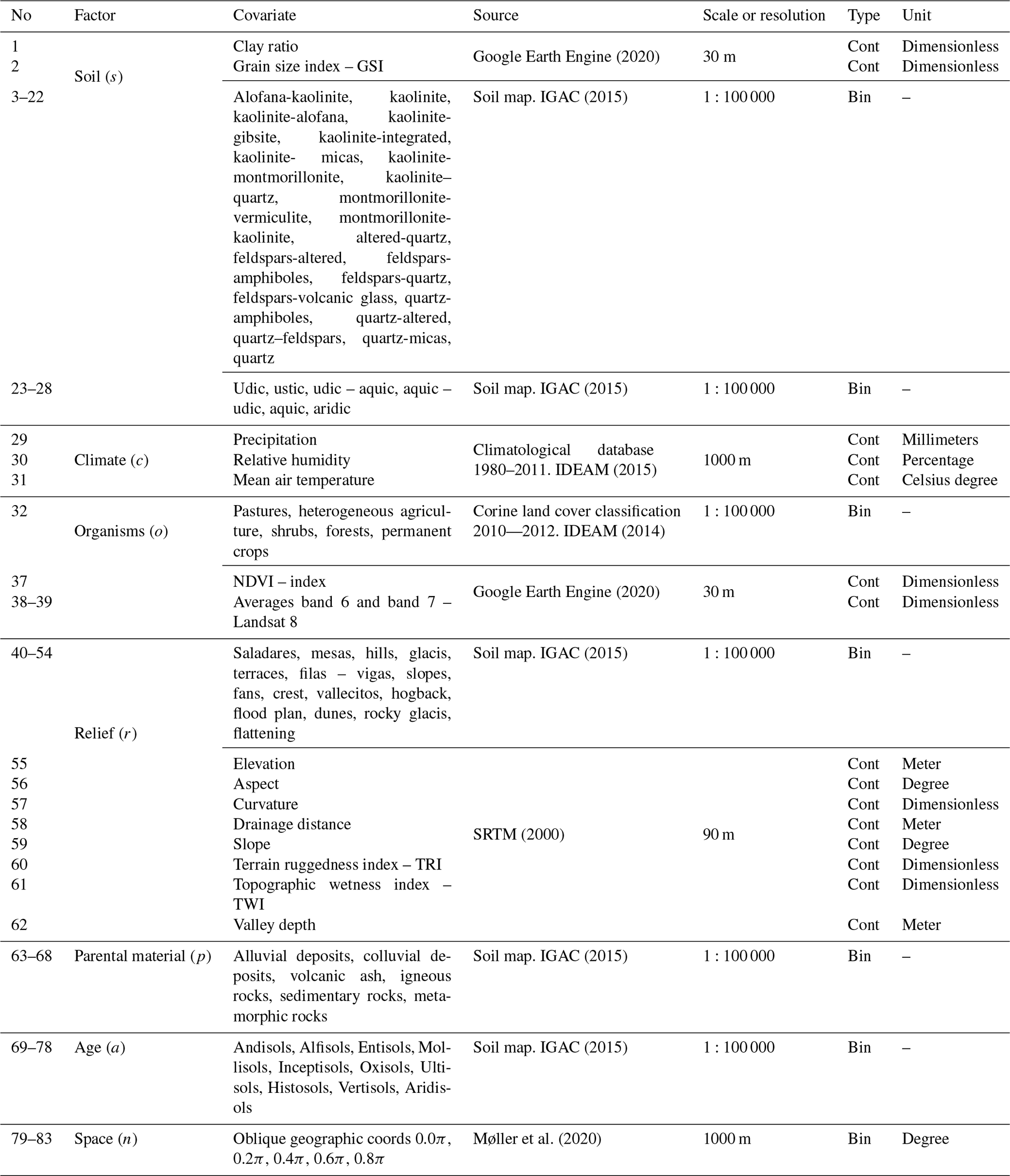
Using ESRI^® ArcGIS™ version 10.3, a total of 83 environmental covariates were selected to broadly reflect soil forming factors, as described by McBratney et al. (2003):

$$\begin{array}{}\text{(3)}& S_{\mathrm{a}}=f(s,c,o,r,p,a,n),\end{array}$$

where a soil attribute (S_a) is a function of other properties of the soil at a point (s), the climate (c), organisms (o), relief (r), parent material (p), age (a), and space (s) (Table 1). The pixel size of the environmental covariates was adjusted to 1 km² using two methods: nearest neighbor and bilinear interpolation. Then, a stack of covariates (collection of rasters) was compiled for Colombia.

IGAC (2015)IGAC (2015)IDEAM (2015)IDEAM (2014)IGAC (2015)IGAC (2015)Møller et al. (2020)

Table 1 Environmental covariates by soil forming factor. Cont: continuous; Bin: binary.

A recursive feature elimination (RFE) was run for each depth and transformation, using the function rfe of the caret package (Kuhn, 2022). The RFE is an algorithm that implements a backward selection of covariates based on predictor importance ranking (Kuhn, 2022). The goal was to find a subset of covariates used to produce the most accurate model possible. A regression matrix for each depth and transformation was built with the selected covariates, and this allowed extraction of the covariate values at the coordinates of each soil sample. With the regression matrix the dataset was divided using the function createDataPartition of the caret package (Kuhn, 2022). This function generates a stratified random split of the data and aims to create balanced splits of the data: a part for model training (75 %) (training samples in Fig. 1) and another independent part for validation purposes (25 %) (testing samples in Fig. 1) (Guevara et al., 2018).

2.4 Prediction models

The spatial distribution of the PSF at each of the five standard depths was modeled through ensemble machine learning (EML) algorithms in two R packages: MACHISPLIN (Brown, 2021) and landmap (Hengl, 2021). EML consists of various approaches based on different methodologies, including stacking methods, averaging methods, bagging, and boosting approaches (Zounemat-Kermani et al., 2021).

MACHISPLIN evaluates different combinations to predict the input data, weighing and evaluating the fit. MACHISPLIN algorithm interpolates multivariate data through EML using six algorithms: boosted regression trees (BRTs), neural networks (NNs), generalized additive model (GAM), multivariate adaptive regression splines (MARS), support vector machines (SVMs), and random forest (RF). This approach evaluates (via k-fold cross validation, where k=10) a method’s ability to predict the input data and ensembles of all combinations of the six algorithms weighting each from 0 to 1. The best model will have the lowest Akaike information criterion with a correction for small sizes. After the best model is determined, the function runs the ensemble on the full dataset. Then, residuals are calculated and interpolated using a thin plate smoothing spline; this creates a continuous error surface and is used to correct most of the residual errors in the final ensemble model (Brown, 2021).

The landmap algorithm applies the stacking ensemble type. Stacking (sometimes called stacked generalization or committee machine approach) learns in parallel and fits a meta-model to predict ensemble estimates (Zhang and Ma, 2012). The “meta-model” is an additional model that combines all individual or “base learners” (Hengl, 2021). The landmap approach ensembles different machine learning algorithms, a fast implementation of RF (ranger), extreme gradient boosting (xgboost), support vector machines (ksvm), neural networks (nnet), and generalized linear models (GLMs) (with Lasso or elastic net regularization). The landmap package extends the functionality of the deprecated mlr “meta-package” (now mlr3) (Lang et al., 2019) and is based on super learner. It is a prediction method designed to find the optimal combination of a collection of prediction algorithms, and its framework is built on the theory of cross-validation and allows for a general class of prediction algorithms to be considered for the ensemble (Polley and Van der Laan, 2010).

The main difference between these two algorithms is the cross-validation. MACHISPLIN randomly makes cross-validation, while landmap makes spatial cross-validation. In the random process, the testing and training dataset would not be independent in this scenario, with the consequence that cross-validation fails to detect a possible overfitting (Lovelace et al., 2019). That situation is performed by landmap, due to it blocking some training points based on spatial dependence (it makes a semivariogram model) to prevent it from producing biased estimations predictions (Hengl, 2021). However, Wadoux et al. (2021b) indicate that spatial cross-validation methods may provide biased estimates of map accuracy, but standard cross-validation is deficient in the case of clustered data. Additionally, MACHISPLIN constructs the best linear model, systematically assigning a weight for each algorithm and evaluating the fit of the ensemble algorithm. In contrast, landmap constructs the meta-model with the predictions of the cross-validation (indicated in the method of ensemble).

2.5 Validation

The validation process had three steps: (i) inclusion of SG layers, (ii) calculation of map quality measures, and (iii) identification of the spatial distribution of the prediction error.

In the first step, one aim of the work was to compare the spatial prediction of techniques mentioned in Sect. 2.4 against the products from SG Version 2.0 (Poggio et al., 2021). In this step, SG layers (250 m pixel size) of the PSF at each standard depth were downloaded.

In the second step, the prediction errors, which is the difference between the predicted value and observed value (Brus et al., 2011), were calculated for each testing sample. After that, were calculated some quantitative statistics: mean error (ME), root mean square error (RMSE), amount of variance explained (AVE), and concordance correlation coefficient (CCC). ME measures bias in the prediction and is defined as the population mean of the prediction errors (Yigini et al., 2018), values close to 0 indicate that the predictions are unbiased. RMSE is a measure of prediction accuracy, and a perfect model would have a value ≈ 0 (Kempen et al., 2012). The AVE measures the fraction of the overall dispersion of the observed values that the model explains, and this measure has an optimal value of 1 (Samuel-Rosa et al., 2015). Finally, the CCC measures the agreement of predicted values with observed values (relationship 1:1), where 1 is a perfect concordance and 0 is no correlation (Lawrence and Lin, 1989).

In the third step, the prediction errors were interpolated using ordinary kriging (OK), a widely used geostatistical technique that assumes intrinsic stationarity (Webster and Oliver, 2007). This process was done for prediction errors of the three approaches (MACHISPLIN, landmap, and SG) in the five standard depths and each PSF. The layers obtained in this step were harmonized according to this study's resolution and extent framework.

2.6 Spatial ensemble

The spatial ensemble maps and their ensemble errors were generated for each depth and PSF (Fig. 2). First, with the error prediction maps for each PSF, a mean absolute error (MAE) was calculated for each EML and SG. After, a spatial ensemble function was created to perform a conditional evaluation using the prediction maps and their respective MAE; at each pixel, the function identified which model (EML or SG) had the minimum MAE and selected the predictions for clay, sand, and silt of it. At last, an ensemble prediction error map was built for each PSF doing a mask by model selected and assigning their respective prediction error (calculated in Sect. 2.5). After, the map quality measures statistics were newly calculated.

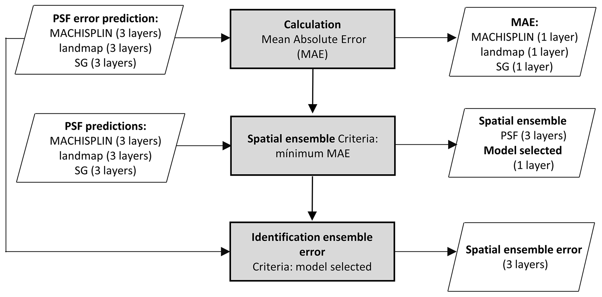
Figure 2 Framework used for generating ensemble maps. PSF means inputs or outputs for clay, sand, and silt.

3 Results

This study represents the first effort to provide a national map of soil texture using a digital soil mapping framework in Colombia. This work used EML algorithms to improve the accuracy of national soil texture predictions, with a fully independent dataset, concerning the global product (SG). Also, it provided new insights for assessing the quality and accuracy of global soil texture predictions. The main results are going to be shown in the following subsections.

3.1 Soil texture characterization and dataset

The textural classes for each sample point at five standard depths are shown in Fig. 3. In most USDA textural classes, the dataset has soil samples. Sandy loam, loam, clay loam, sandy clay loam, and clay were the most frequent textural classes in all standard depths, and silty and silty loam textural classes were less frequent. Also, it is easy to identify that, in the dataset, there are not many soil samples with high content of clay and silt, while extreme contents of sand fraction are frequent.

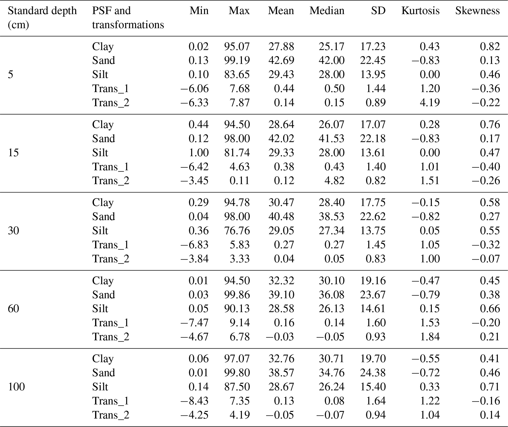
Descriptive statistics are shown in Table 2 for PSF and its transformations (Trans_1 and Trans_2). The PSF covers the entire range of measures (0 % to 100 %), which is expected for national-scale analysis. The mean and median for sand fraction was higher than clay and silt fractions in all standard depths, indicating that sand is the dominant PSF in Colombian soils. The standard deviation grew for all fractions in the deepest layers; sand content was the fraction with the highest variation in all depths. These results suggest that sand fraction has the highest variability in the PSF for Colombian soils, which rises with increasing depth. The skewness coefficients were positive and less than 1 for all textural fraction dataset, and the sand fraction showed less deviation from the normal distribution, except for 60–100 cm layer. Regarding transformations, the ranges took values from negatives to positives with means around zero; this signifies that ALR transformation improved the sand and silt distribution for all depths, except the sand in the first three layers.

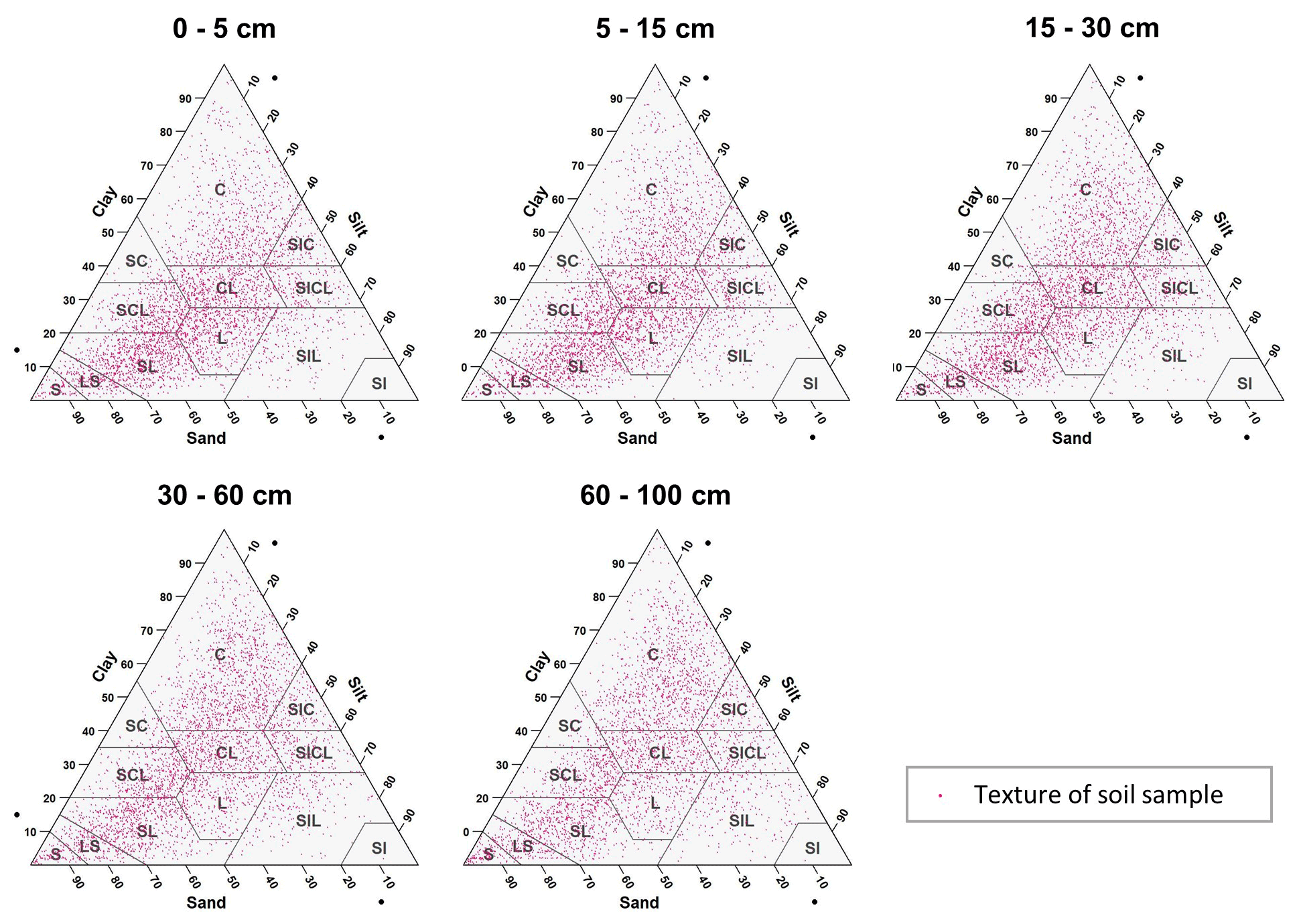
Figure 3 Particle size soil samples representation in a textural diagram for each standard depth. C: clay, SC: sandy clay, SCL: sandy clay loam, CL: clay loam, SIC: silt clay, SICL: silt clay loam, L: loam, SIL: silt loam, SI: silt, SL: sandy loam, LS: loamy sand, and S: sand.

Table 2 Descriptive statistics of PSF and its transformations for each standard depth. Min: minimum; Max: maximum; SD: standard deviation.

3.2 Covariate selection

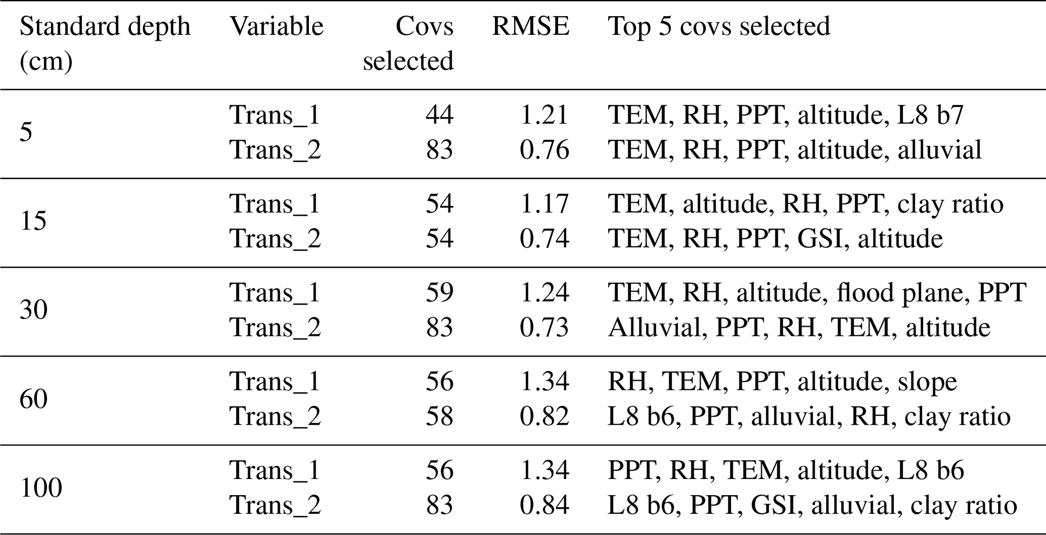
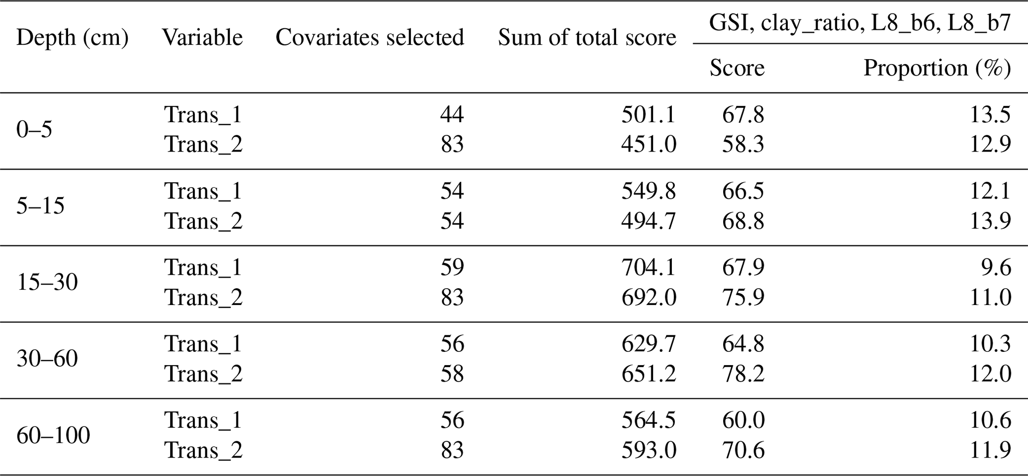
Ten recursive feature elimination models were obtained, and individual covariate stacks were built for each transformation in all standard depths. For each layer, covariates were selected for Trans_1 and Trans_2, respectively: 44 and 83 (0–5 cm), 54 and 54 (5–15 cm), 59 and 83 (15–30 cm), 56 and 58 (30–60 cm), and 56 and 83 (60–100 cm) (Table 3). The top 5 covariates (Table 3) included soil forming factors: climatic (temperature, relative humidity, and precipitation), topographic (altitude, slope, and presence of flood planes), parent material (presence of alluvial deposits), activity of organisms (bands 6 and 7 of Landsat 8) and previous soil index information (clay ratio and grain size index). It is important to highlight that the covariates selection had only two binary covariates (alluvial and flood plains).

3.3 Soil texture predictions and SG products validation

Map quality measures are given in Table 4. Referring to ME, silt fraction was overestimated (positive ME), and clay and sand fractions were underestimated (negative ME); this happened for all depths and EML algorithms, except clay in 60–100 cm layer. For sand fraction, the bias values of landmap predictions were fewer than MACHISPLIN predictions. The ME values closets to zero were found for clay in the deepest layer, suggesting unbiased predictions for both MACHISPLIN and landmap algorithms. Comparing MACHISPLIN and landmap, the RMSE values were similar for each PSF and depth. However, comparing RMSE values between PSF, RMSE values for sand were always higher than clay and silt.

The AVE values were under 0.35. For all standard depths and algorithms, sand fraction had higher AVE values than clay and silt, except in the 60–100 cm layer, where AVE values for clay were higher. In general, for MACHISPLIN and landmap, the capacity of each model to explain the variance decreased when increasing depth; however, it is important to highlight the AVE values for silt fraction in 0–5 and 5–15 cm layers, which were so close to zero. On the other hand, the CCC values were from 0.32 to 0.54. The CCC values for sand were higher than clay and silt in all cases. Also, the lowest CCC value between standard depths was found in the deepest layer (60–100 cm), where the data set had fewer sample points than the superficial layers. These results suggest that, for sand, the predicted and observed values agree more than the clay and silt fraction.

An evaluation of SG products with the dataset validation (the same used for EML validation) is shown in Table 4. About ME, the highest bias values were found for sand fraction, followed by clay and silt. For sand fraction, the estimations were underestimated (negative ME) in all standard depths; in contrast, for clay and silt fractions, the estimations were overestimated (positive ME), except by silt in 30–60 cm layer. These ME values were higher than EML predictions. Concerning RMSE values, the sand fraction had higher values than the clay and silt fraction, and the RMSE increased with increasing depth. For AVE, negative and close to zero values were found in all standard depths and fractions (−0.27 to −0.08). Similarly, the CCC values were close to zero (0.04 to 0.16), and the highest values were obtained for sand and silt fraction in the three most superficial layers.

In Fig. 4 there is a visual comparison of our results and SG products. In this representation, we can see some aspects: first, the ranges of the predicted values are wider for MACHISPLIN and landmap than SG (low contrast of colors). Second, the general pattern of PSF distribution is different between our results and SG products. Principally, in the Andean and Caribbean regions, our results suggest that these areas have higher values of sand (blue colors) than clay and silt fractions, while SG suggests soils with more content of clay and silt (orange and green colors); also, in Orinoquia region, our results show soils with high content of silt (green colors) and SG displays soils with more content of clay and sand (purple colors). Third, in the southern and eastern areas, the SG products do not have artifacts generated for the prediction of the algorithms; this is an advantage of SG products.

Table 3 Top five covariates selection for each transformation and standard depth. TEM: temperature, RH: relative humidity, PPT: precipitation, L8 b7: Landsat 8 band 7, L8 b6: Landsat 8 band 6, GSI: grain size index.

3.4 Spatial ensemble

Figures 5 to 9 display the final spatial ensemble maps for each PSF, which contain their final error and the model selected for each pixel at each standard depth. The spatial ensemble, which, as described above, is a collection of best-fit data from three different algorithms (MACHISPLIN, landmap, and SG), contained common elements/features in most standard depths.

In all standard depths, predictions of MACHISPLIN (yellow color) and landmap (green color) represented the PSF distribution more than SG (gray color). The SG selection increased with depth, especially in 60–100 cm layer. The most significant areas where SG had the fewest prediction errors were in Orinoquia and Amazon regions. Similar to SG, the landmap predictions were frequently selected in the deepest layers overall in the southern areas of Colombia. MACHISPLIN predictions were most chosen in the areas with the lowest sample density (Orinoquia and Amazon regions).

Concerning PSF distribution, sand fraction had the highest variation in the geographical space in all depths. The highest mountains in the central areas, the Sierra Nevada in the northern, and the hills in the eastern areas had a significant content of sand; in contrast, the finest fractions (clay and silt) were found mainly in valley landscapes between mountain chains in central areas of Colombia and hill landscape in the eastern areas.

The external validation for the spatial ensemble maps showed an improvement in their metrics vs. the maps using EML algorithm or SG product (Table 5). The ME values were closer to zero, showing an improvement in the prediction; however, in this ensemble model, predictions of silt fraction had the highest bias, which is a different behavior of EML algorithms (MACHISPLIN and landmap), where sand fraction had the most biased predictions. RMSE values decreased for all PSF and standard depths, which means a raising in the precision of the map. On the other hand, AVE values increased with the spatial ensemble model; interesting that the AVE values for silt fraction at 0–5 and 5–15 cm were higher compared to landmap predictions (Table 4); also the sand fraction had the most betterment respect to clay and silt fraction. Concerning CCC values, these are still equal to or higher than individual algorithms.

Table 4 Map quality measures of each algorithm for PSF in five standard depths. ME: mean error; RMSE: root square mean error; AVE: amount of variance explained; CCC: concordance correlation coefficient. These map quality measures are based on the validation dataset.

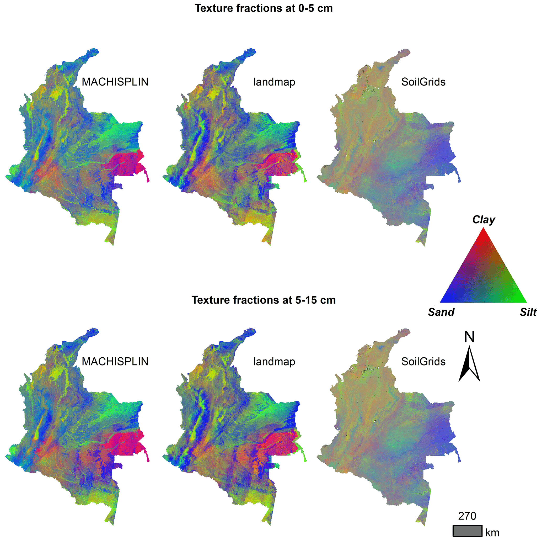
Figure 4 Color composite map of soil texture fractions predictions at two depths: 0–5 and 5–15 cm.

Table 5 Summary of map quality measures for spatial ensemble model for PSF in five standard depths. ME: mean error; RMSE: root mean square error; AVE: amount of variance explained; CCC: concordance correlation coefficient. These map quality measures are based on the validation dataset.

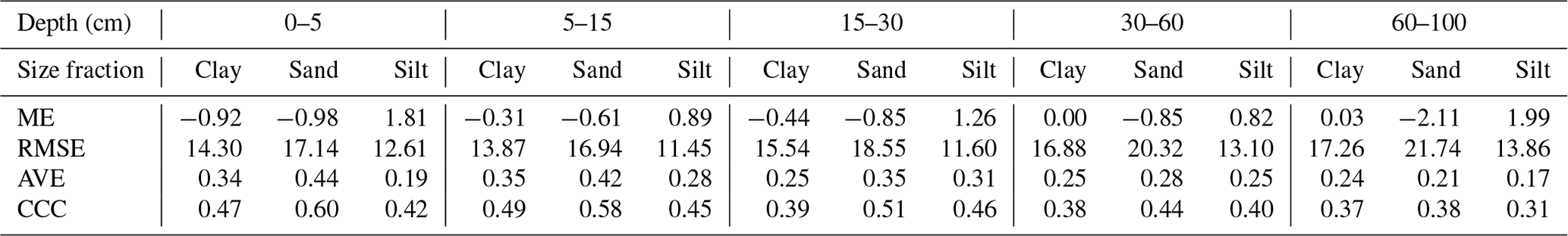
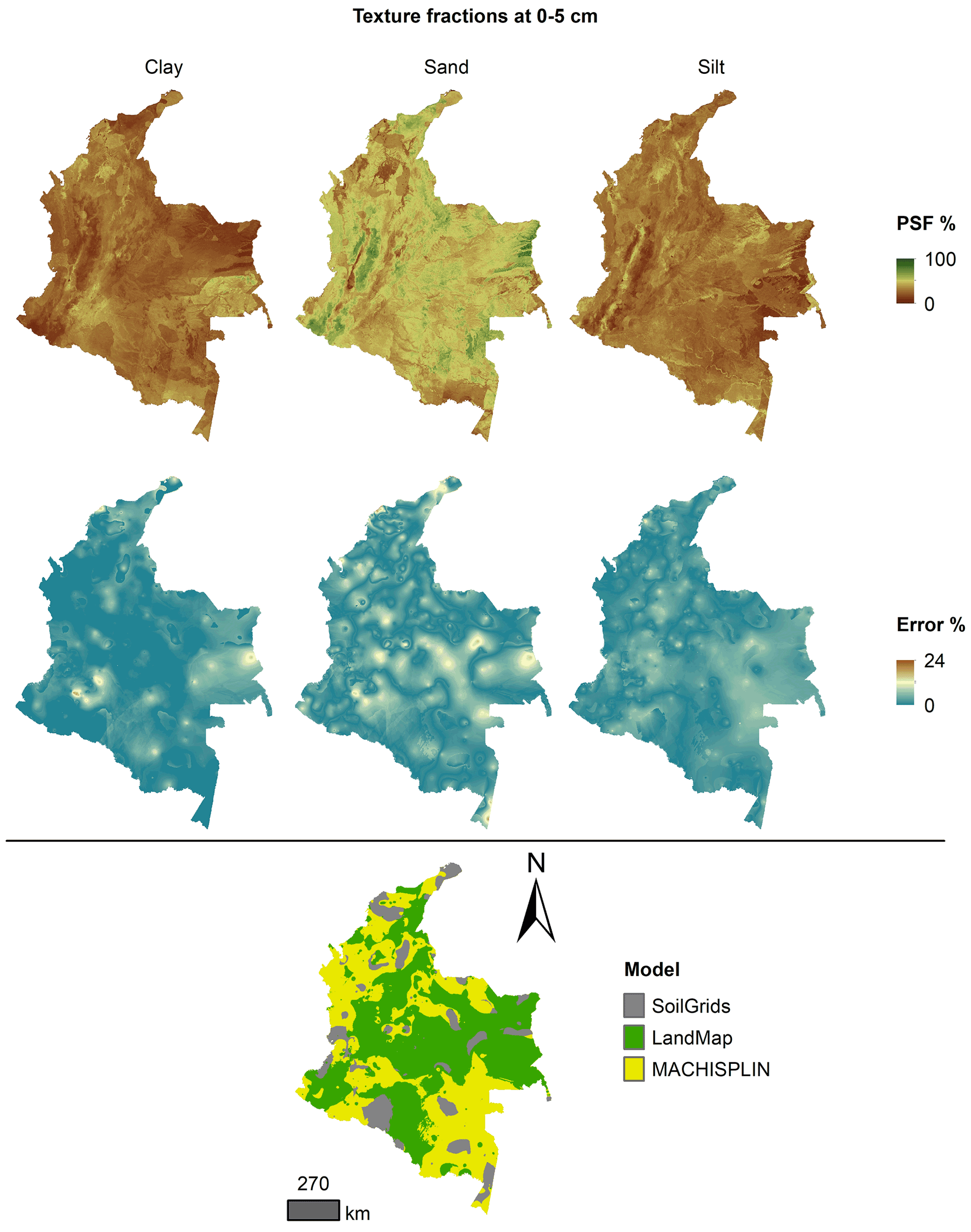
Figure 5 Ensemble model, percentage error distribution, and best model selected at 0–5 cm.

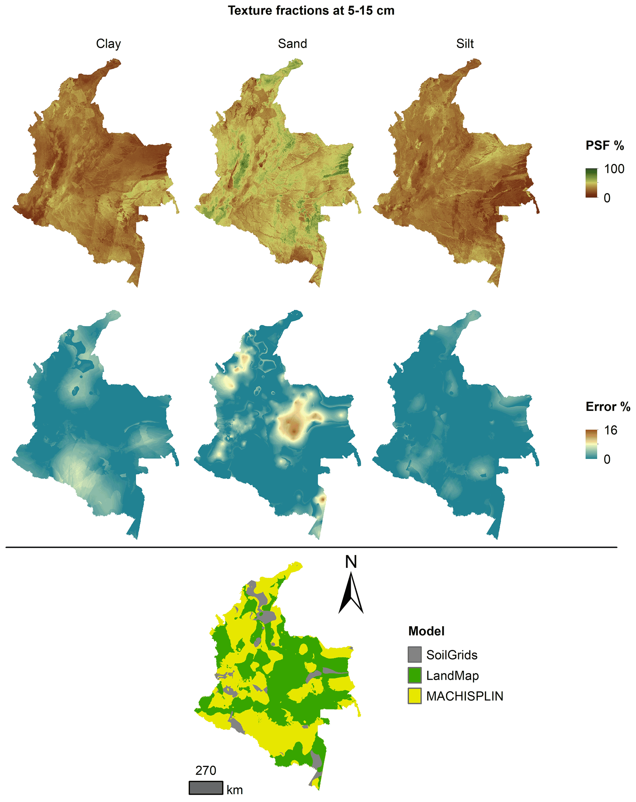
Figure 6 Ensemble model, percentage error distribution, and best model selected at 5–15 cm.

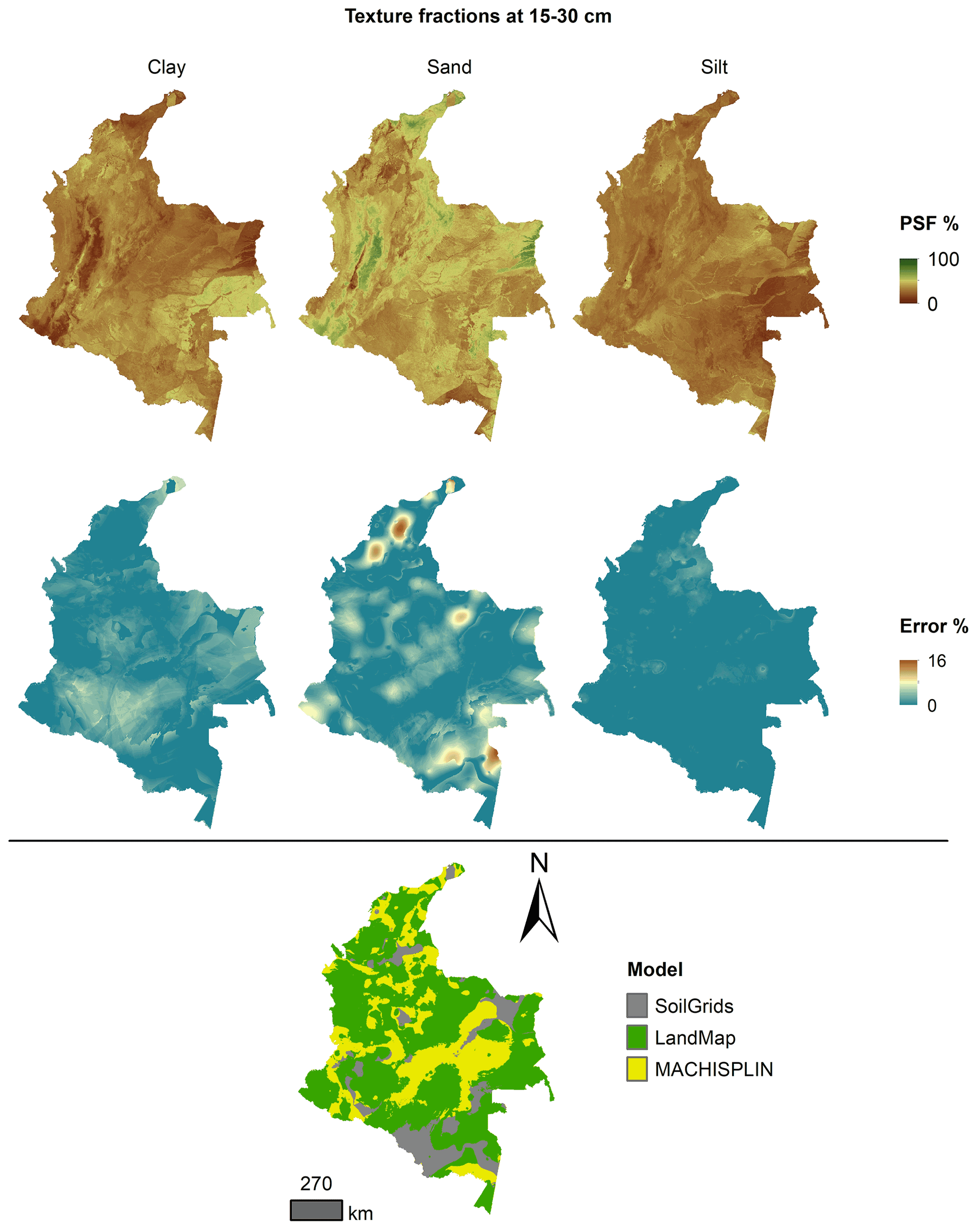
Figure 7 Ensemble model, percentage error distribution, and best model selected at 15–30 cm.

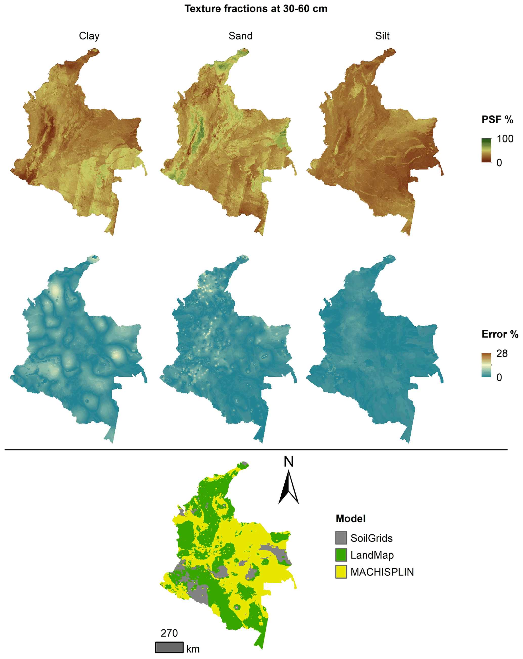
Figure 8 Ensemble model, percentage error distribution, and best model selected at 30–60 cm.

Figure 9 Ensemble model, percentage error distribution, and best model selected at 60–100 cm.

4 Discussion

In this paper, we developed a new digital soil texture dataset that contains legacy soil data, environmental covariates, and the first digital soil texture maps across Colombia. Colombia's literature on machine learning applied to soil texture mapping is limited. We improved the accuracy and spatial resolution of previous conventional maps. While many studies focus on mapping soil properties such as pH and organic matter, fewer studies focus on comparing and testing global approaches, such as SoilGrids, for maximizing accuracy. Our results contribute to a national benchmark of the reliability of global predictions compared to national predictions. We first discuss the general geography of soil texture across the country and compare and discuss our findings with previous work.

Colombia has a great diversity of soils, and their properties change with depth. In the five standard depths, soil texture in Colombia has representation in all textural classes defined by Soil Survey Staff (2014). As depth increases, the soil texture is finer, and the proportion of clay and silt rises. On the other hand, coarse soils are in central and northern areas, and these soil textures hold with increasing depth. This high diversity of soil texture is due to the high number of interactions between soil forming factors, particularly the great diversity of parent materials within Colombia (IGAC, 2015; Araujo et al., 2017).

Some topography and parent material covariates were the principal drivers in texture modeling. The focal areas with fine and medium textures are found in the northwest (floodplain and land depressions), in central areas (Magdalena River valley), in the west (Cauca River valley), in the south (Amazon region), and the east (Orinoquia region). All these regions have specific soil forming factors, such as alluvial parent material deposited by one or many rivers, which are soil fine-size fractions driver, Flórez, 2003). On the other hand, medium and coarse textures are principally in the hillsides of mountain landscapes in central, southern, and southwestern regions. Mainly, these coarse soil textures are due to the presence of sandstone, conglomerate sandstone, granites, and gneisses, among others, that have siliceous and quartz rocks (Catoni et al., 2016), volcanic materials, and glacial clast (IGAC, 2015) that are in these areas. Despite the relationship between soil texture distribution, relief, and parent material covariates, only altitude (quantitative), slope (quantitative), alluvial (binary), and flood plane (binary) covariates were present in the top five predictors for each standard depth.

Although parental material is critical in the soil texture spatial distribution, the covariates selection identified that the climatic covariates were more important (i.e., temperature, relative humidity, and precipitation). The covariates used to describe the parental material were binary class variables; maybe the following exercises should include quantitative variables to identify this soil forming factor, for example, using radar remote sensing (Niang et al., 2014) or based on the spectral response in the visible and near-infrared spectrum (Vis-NIR), medium infrared (MIR), and Vis-NIR-MIR (Campbell et al., 2019). In the PSF predictions (in specific, the ALR components), the importance of the climatic covariates did not have apparent changes with depth. The country's climate conditions have led to relatively strong physical weathering in the soil forming process (Osman, 2013). Due to the country's location, it is influenced climatologically by the atmospheric circulation of the Caribbean Sea, Pacific Ocean, the Amazon Basin, and the orographic barrier of the three branches of the Andes Mountains (Poveda, 2004). Furthermore, in this study, the variables were chosen to maximize the predictive power of the models, not their explanatory capabilities.

Colombia has not produced maps on PSF at a national scale with DSM products, but Colombia has developed soil surveys through conventional mapping (IGAC, 2015); then, the textural soil distribution of Colombia presented in this study is not directly comparable with previous national textural soil maps. Due to the methodology used in IGAC (2015), the depth studied is different, the polygons delineated (CSU) have a unique value for an entire area, and CSUs are not an uncertainty value associated. These last two reasons are the primary use limitations in traditional soil surveys (Angelini et al., 2016). Despite that, the maps produced by this study and those of the IGAC project show two significant areas with similar attributes. In the northwest (Caribbean region) and south (Amazon region), the IGAC study presents a fine group texture (clay between 40 % and 60 %), and this current result shows that levels of clay percentages are in that clay range. However, there is a principal region in the west (Orinoquia region), where the two results are very different. The previous result shows these areas with a coarse textural group, and this current result displays low percentages of sand fractions for 5–15, 15–30, and 30–60 cm depths. These differences are due to the low soil sampling density, where there is just one observation, and in this current study, its nearest predictions are driven by soil data.

Regarding map quality measures, RMSE had the highest values for the sand fraction. This is the same behavior found by other studies that implemented different algorithms (geostatistics and machine learning) (Poggio and Gimona, 2017; Laborczi et al., 2019; Liu et al., 2020); however, the joint statement in those studies was that, for sand fraction, the ranges were wider and the SD was higher compared with clay and silt fraction. The CCC values for sand were higher than clay and silt in all cases, and this is the same behavior found by Mulder et al. (2016) in France. Additionally, for all PSF, they found that the predictions were less reliable for deepest layers; this is the same statement found in this work. Their map quality measures are better than ours; however, the soil samples used in that work were between 28 000 and 3000, decreasing with increasing depth.

The qualitative evaluation for SG at a global scale showed that coarse-scale patterns are well reproduced (Poggio et al., 2021). Nevertheless, in a quantitative evaluation with Colombian soils, SG products cannot explain the variance (AVE values negative), their predictions are not according with our validation dataset (CCC is not close to zero), and their RMSE values are significantly higher than ours. Liu et al. (2020) built a national map of silt in China, and they compared their results with SG products through RMSE values. They found that their RMSE values were higher than the RMSE of SG, and in many specific areas, SG did not represent the local behavior of the PSF. In this way, we suggest, for applications that need textural soil information at a national scale, to use our results obtained with individual algorithms (MACHISPLIN and landmap) and the ensemble maps. However, it is important to point out that in some areas of Orinoquia and Amazon region, the SG had the fewest prediction error; these regions had a low soil sampling density in common.

This work could identify the PSF's better models, error trends, and prediction layers. However, in many areas, depths, and textural fractions, the map quality measurements are low; for example, we desire to increase AVE and CCC values. The causes can be many: the relations between some soil properties and landscape attributes are nonlinear, complex, or unknown, a concept defined by Minasny and McBratney (2010). Linked to the aforementioned is the distribution of the soil samples. The study had an unbalanced representation and spatial clustering; for example, the central zone (Andean region) was the most represented (bias towards potentially productive areas), while the east and southeast zones were the least represented, so many predictions were largely controlled by point data, then, some large artifacts (e.g., lines and blocky outputs) are shown in these areas, a similar case to that reported by Hengl et al. (2014). These artifacts are derived mainly from covariates related to satellite images, such as bands 6 and 7 from Landsat 8, and its derivatives (clay ratio and grain size index). These four covariates were obtained from Google Earth Engine with seam carving and had a significant importance in the RFE model, and their score importance (overall in RFE model) is between 10 % and 14 % with respect to the best subset of covariates (Appendix A1). Additionally, for agricultural studies, the use of these results will be straitened to the agricultural limit defined in Colombia, places where the results do not have artifacts (Appendix A2).

In Colombia, DSM has great challenges to attend map-user's requirements, such as soil texture predictions with uncertainty improvements and soil maps with better spatial resolution. There are three principal strategies to improve predictions: treatment of unbalanced soil data, management of PSF transformations, and incorporation of new environmental covariates related to soil texture drivers. Attending to the first strategy is necessary to raise the soil database with available soil information from other sources such as detailed soil surveys, soil degradation, and soil management studies made by national and governmental institutions (e.g., IGAC, IDEAM, or UPRA); or obtaining the amount of each fraction from other kinds of soil analysis, such as visible near infrared short of soil minerals (Lagacherie et al., 2020). Also, model-building processes by soil groups (Kempen et al., 2009) or homosoil (Mallavan et al., 2010; Angelini et al., 2020; Malone et al., 2016) have been used to get pedologically plausible predictions in areas without high soil sampling density. Other log ratio transformations could be applied as a second strategy to improve ALR transformation issues. For example, Wang and Shi (2017) indicated that in some datasets, the changes in the denominator selection in additive log ratio transformation could represent different predictions and decrease the accuracy of the estimates. Then, using centered log ratio transformation, this issue could be avoided (Amirian-Chakan et al., 2019). Also, data sets with zero values must be threatened with symmetry and isometric log ratio transformation (Li et al., 2020). Finally, as a third strategy, some qualitative and quantitative environmental covariates could buttress the predictors' stack, such as depth to bedrock and soil horizons designations and thickness. Also, to improve the visual quality of the results, a previous covariate analysis could be used, such as principal components (Hengl et al., 2014), or a smoothed strategy.

5 Code and data availability

Training and testing data are available at https://doi.org/10.6073/pasta/3f91778c2f6ad46c3cc70b61f02532db (Varón-Ramírez and Araujo-Carrillo, 2022). This repository contains the data set for each standard depth. For each sample point, PSF and ALR transformations are shown (Trans_1 and Trans_2).

Textural soil maps are available at https://doi.org/10.6073/pasta/d6c0bf5847aa40836b42dcc3e0ea874e (Varón-Ramírez et al., 2022). In this repository, the users are going to find nine raster stacks: PSF obtained with landmap and MACHISPLIN algorithms (two stacks); PSF obtained from SG (one stack); residual of the PSF predictions for landmap and MACHISPLIN algorithms and SG (three stacks); PSF predictions obtained through a spatial ensemble technique (three stacks). All stacks contain information at five standard depths.

Rproject scripts to reproduce the spatial ensemble procedure and models validation area are available at https://doi.org/10.5281/zenodo.7185675 (VimiVaron, 2022).

6 Conclusions

We provided the first comparison of the PSF across Colombia between EML models (MACHISPLIN and landmap) and SG's existing soil texture maps. The study shows that the spatial distribution of soil texture prediction with national datasets was, on average, 17 % better (in terms of RMSE) using EML models than the SG products. Between MACHISPLIN and landmap, there was no better EML model because the quantitative statistics were very similar. In function of the PSF, the spatial distributions did not exhibit a fraction with better results. However, layers of 0–5, 5–15, and 15–30 cm obtained the best results, which indicate the effectiveness in the depths closest to the soil surface.

Another valuable contribution developed in this study was the implementation of the spatial ensemble of soil texture fractions on a national scale and at different depths. This implementation identified the best result for each depth and each pixel. Although the SG products had the worst quantitative statistics, in some areas of the country, these products performed well, mainly in the south. However, with the spatial ensembles, the best composition of the models was possible.

The spatial distribution of soil particle size fractions can provide soil information for water-related applications, ecosystem services, and agricultural and crop modeling. However, the results had limitations, especially with some artifacts in the southern and eastern areas. Treatment of unbalanced soil data and incorporation of more appropriate environmental covariates are crucial to improving accuracy in the future.

Appendix A

A1 Importance of covariates in recursive feature elimination for Trans_1 and Trans_2 prediction

Table A1 Representation of importance scores for satellite-derived covariates. GSI: grain size index, L8 b7: Landsat 8 band 7, L8 b6: Landsat 8 band 6.

Appendix B

B1 Agricultural frontier in Colombia

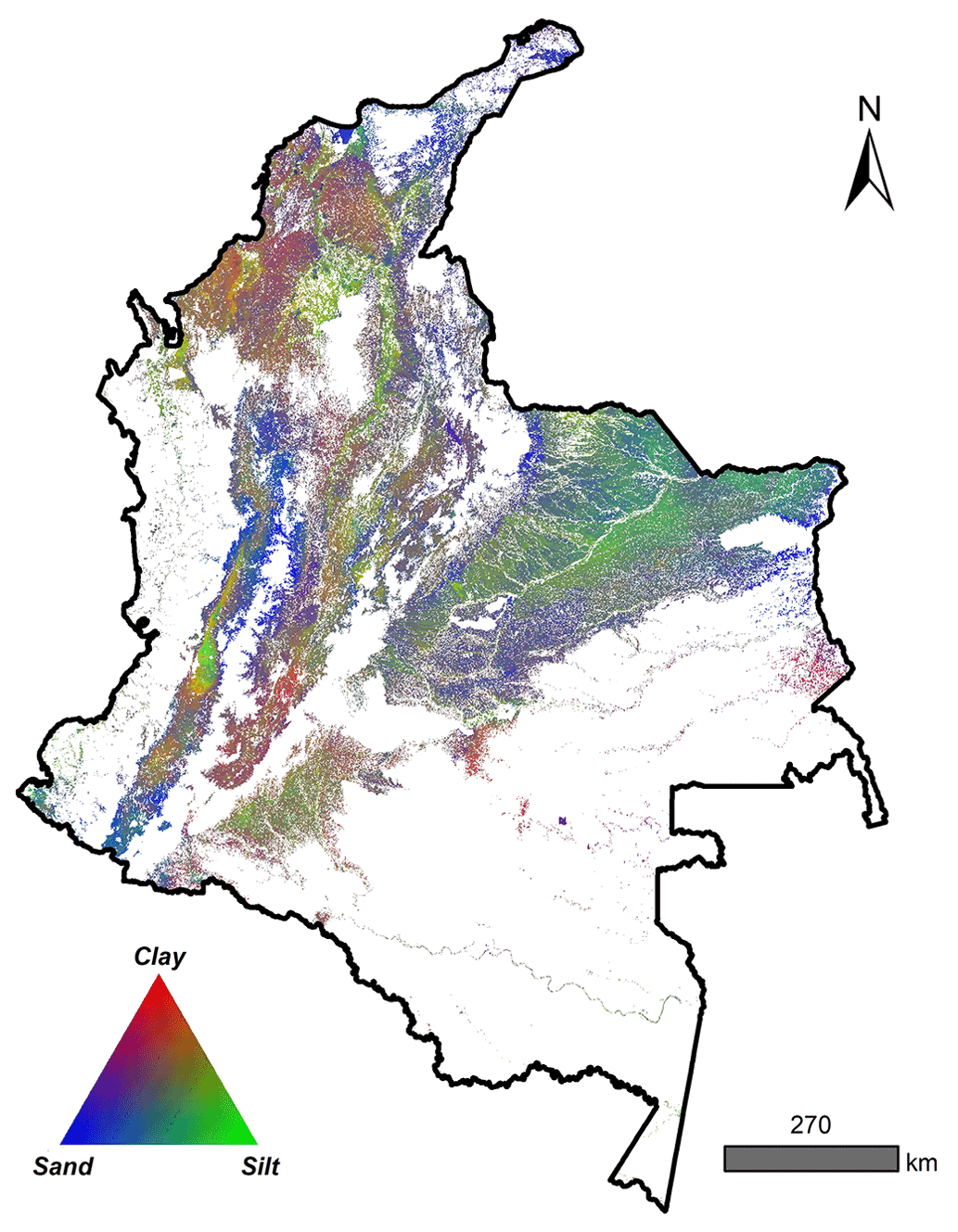
Figure B1 Compositional texture map (clay, sand, and silt), integrated from 0 to 100 cm, in the agricultural frontier in Colombia.