the Creative Commons Attribution 4.0 License.
the Creative Commons Attribution 4.0 License.
 | 21 Oct 2022
Quality control and correction method for air temperature data from a citizen science weather station network in Leuven, Belgium
Maarten Reyniers
Raf Aerts
Ben Somers
The growing trend toward urbanisation and the increasingly frequent occurrence of extreme weather events emphasise the need for further monitoring and understanding of weather in cities. In order to gain information on these intra-urban weather patterns, dense high-quality atmospheric measurements are needed. Crowdsourced weather stations (CWSs) could be a promising solution to realise such monitoring networks in a cost-efficient way. However, due to their nontraditional measuring equipment and installation settings, the quality of datasets from these networks remains an issue. This paper presents crowdsourced data from the “Leuven.cool” network, a citizen science network of around 100 low-cost weather stations (Fine Offset WH2600) distributed across Leuven, Belgium ( N, E). The dataset is accompanied by a newly developed station-specific temperature quality control (QC) and correction procedure. The procedure consists of three levels that remove implausible measurements while also correcting for inter-station (between-station) and intra-station (station-specific) temperature biases by means of a random forest approach. The QC method is evaluated using data from four WH2600 stations installed next to official weather stations belonging to the Royal Meteorological Institute of Belgium (RMI). A positive temperature bias with a strong relation to the incoming solar radiation was found between the CWS data and the official data. The QC method is able to reduce this bias from 0.15 ± 0.56 to 0.00 ± 0.28 K. After evaluation, the QC method is applied to the data of the Leuven.cool network, making it a very suitable dataset to study local weather phenomena, such as the urban heat island (UHI) effect, in detail. (https://doi.org/10.48804/SSRN3F, Beele et al., 2022).
- Article
(30570 KB) - Full-text XML
- BibTeX
- EndNote


More than 50 % of the world's population currently lives in urban areas, and this number is expected to grow to 70 % by 2050 (UN, 2019). Keeping this growing urbanisation trend in mind and knowing that both the frequency and intensity of extreme weather events will increase (IPCC, 2021), it becomes clear that both cities and their citizens are vulnerable to climate change. To plan efficient mitigation and adaptation measures and, hence, mitigate future risks, information on intra-urban weather patterns is needed (Kousis et al., 2021). Therefore, dense high-quality atmospheric measurements are becoming increasingly important to investigate the heterogeneous urban climate. However, due to their high installation and maintenance costs as well as their strict siting instructions (WMO, 2018), official weather station networks are sparse. As a result, most cities only have one official station, or they may even lack an official station (Muller et al., 2015). Belgium only counts around 30 official weather stations distributed across a surface area of 30 689 km2; a total of 18 of these weather stations (Sotelino et al., 2018) are owned and operated by the Royal Meteorological Institute of Belgium (RMI). These classical observation networks operate at a synoptic scale and are, thus, not suitable to observe city-specific or intra-urban weather phenomena such as the urban heat island (UHI) effect (Chapman et al., 2017).
The UHI can be measured using a number of methods. Fixed pairs of stations (e.g. Bassani et al., 2022; Oke, 1973) or mobile transect approaches (e.g. Kousis et al., 2021) have traditionally been used to quantify this phenomenon. However, both methods are not ideal: pairs of stations lack detailed spatial information, whereas transects often miss a temporal component (Chapman et al., 2017; Heaviside et al., 2017). Other studies have quantified the UHI using remote sensing data derived from thermal sensors. Such methods can provide spatially continuous data over large geographical extents but are limited to land surface temperatures (LSTs) (Arnfield, 2003; Qian et al., 2018). As opposed to LSTs, the canopy air temperature (Tair) is more closely related to human health and comfort (Arnfield, 2003). Nevertheless, finding the relationship between LST and Tair is known to be rather difficult, and results have been inconsistent (Yang et al., 2021). Numerical simulation models (e.g. UrbClim, De Ridder et al., 2015; SURFEX, Masson et al., 2013) in which air temperature is continuously modelled over space and time could be a possible solution. However, these models still have some drawbacks: due to the computational power capacity, these models only take a limited number of variables into account, making them less suitable for real-life applications (Rizwan et al., 2008); additionally, they often lack observational data to train and validate their simulations (Heaviside et al., 2017).
The rise of crowdsourced air temperature data, especially in urban areas, could be a promising solution to bridge this knowledge gap (Muller et al., 2015). Such data are obtained via a large number of nontraditional sensors, mostly set up by citizens (i.e. citizen science) (Muller et al., 2015; Bell et al., 2015). Crowdsourced datasets have already been successfully used for monitoring air temperature (Chapman et al., 2017; de Vos et al., 2020; Fenner et al., 2017; Napoly et al., 2018; Meier et al., 2017; Hammerberg et al., 2018; Feichtinger et al., 2020), rainfall (de Vos et al., 2019, 2020, 2017), wind speed (Chen et al., 2021; de Vos et al., 2020) and air pollution (EEA, 2019; Castell et al., 2017) within complex urban settings. However, due to their nontraditional measuring equipment and installation settings, the quality of datasets from these networks remains an issue (Bell et al., 2015; Napoly et al., 2018; Chapman et al., 2017; Meier et al., 2017; Muller et al., 2015; Cornes et al., 2020; Nipen et al., 2020). Quality uncertainty arises due to several issues: (1) calibration issues in which the sensor could be biased either before the installation or due to drift over time, (2) design flaws in which the design of the station makes it susceptible to inaccurate observations, (3) communication and software errors leading to incorrect or missing data, (4) incomplete metadata (Bell et al., 2015), and (5) unsuitable installation locations (Feichtinger et al., 2020; Cornes et al., 2020).
Recent studies have, therefore, highlighted the importance of performing data quality control in data processing applications (Båserud et al., 2020; Longman et al., 2018), especially before analysing crowdsourced air temperature data (Bell et al., 2015; Jenkins, 2014; Chapman et al., 2017; Meier et al., 2017; Napoly et al., 2018; Cornes et al., 2020; Nipen et al., 2020; Feichtinger et al., 2020). Jenkin (2014) and Bell et al. (2015) both conducted a field comparison in which multiple crowdsourced weather stations (CWSs) were compared with official (and thus professional) observation networks. Both found a profound positive instrument temperature bias during daytime with a strong relation to the incoming solar radiation. Thus, the use of crowdsourced data requires quality assurance and quality control (QA/QC) in order to both remove gross errors and correct station-specific instrument biases (Bell et al., 2015). Using the findings of Bell et al. (2015) as a basis, Cornes et al. (2020) corrected crowdsourced air temperature data across the Netherlands using radiation from satellite imagery and background temperature data from official stations belonging to the Royal Netherlands Meteorological Institute (KNMI). To investigate the UHI in London, UK, Chapman et al. (2017) used Netatmo weather stations and removed crowdsourced observations that deviated from the mean of all stations by more than 3 standard deviations. Meier et al. (2017) developed a detailed QC procedure for Netatmo stations using reference data from two official observation networks in Berlin, Germany. The QC consists of four steps, each identifying and removing suspicious temperature data. Their methods highlight the need for standard, calibrated and quality-checked sensors in order to assess the quality of crowdsourced data (Cornes et al., 2020; Chapman et al., 2017; Meier et al., 2017). Such official sensors are, however, not present in most cities, hindering the transferability of these QC methods. To this end, Napoly et al. (2018) developed a statistically based QC method for Netatmo stations that was independent of official networks (the CrowdQC R package). The QC method was developed on data from Berlin (Germany) and Toulouse (France), and it was later applied to Paris (France) to demonstrate the transferability of this method. The procedure consists of four main and three optional QC levels, removing suspicious values, correcting for elevation differences and interpolating single missing values. As the CrowdQC-filtered dataset still contained some radiative errors, Feichtinger et al. (2020) combined the methods of Napoly et al. (2018) and Meier et al. (2017) to study a high-temperature period in Vienna in August 2018. Most recently, Fenner et al. (2021) presented the CrowdQC+ QC R package, which is a further development of the existing CrowdQC package developed by Napoly et al. (2018). The core enhancements deal with radiative errors and sensor response time issues (Fenner et al., 2021).
Current QC studies mostly identify and remove implausible temperature measurements (Chapman et al., 2017; Meier et al., 2017; Napoly et al., 2018), instead of correcting for known temperature biases (Cornes et al., 2020). We do, however, know that both the siting and the design of CWSs can introduce such a bias. By parameterising this bias, it can be learned and corrected for, thereby limiting the number of observations that is eliminated (Bell et al., 2015). Additionally, most QC procedures require data from official networks (Cornes et al., 2020; Chapman et al., 2017; Meier et al., 2017), although most cities do not have such measurements available (Muller et al., 2015). Lastly, previous research has also noted that biases can be station-specific; this is because the design of a CWS is an important uncertainty source (Bell et al., 2015), and it indicates the need for station-specific quality control methods. Thus, there is a need for station-specific quality control and correction methods, independent of official weather station networks.
Here, we report on a statistically based QC method for the crowdsourced air temperature data of the “Leuven.cool” network, a citizens science network of around 100 weather stations distributed across private gardens and (semi-) public locations in Leuven, Belgium. The Leuven.cool network is a uniform network in the sense that only one weather station type (Fine Offset WH2600) is used for the entire network. To our knowledge, no quality control method has been developed for this sensor type. The stations were installed following a strict protocol, lots of metadata are available, and both the dataflow and station siting are continuously controlled. This novel QC method removes implausible measurements, while also correcting for inter-station (between-station) and intra-station (station-specific) temperature biases. The QC method only needs an official network during its development and evaluation stage. Afterwards, the method can be applied independently of the official network that was used in the development phase. Transferring the method to other networks or regions would require the recalibration of the QC parameters. After applying this quality control and correction method, the crowdsourced Leuven.cool dataset becomes suitable to monitor local weather phenomena such as the urban heat island (UHI) effect.
The paper is organised as follows. Section 2 describes materials and methods, providing information on the study area, the crowdsourced (Leuven.cool) dataset and the official reference dataset. The development of the quality control method is explained in Sect. 3. In Sect. 4 the newly developed QC method is first tested on four crowdsourced stations installed next to three official stations from the Royal Meteorological Institute of Belgium (RMI). This allows us to quantify the data quality improvement after every QC level. In Sect. 5 the QC method is applied to a network of CWSs in Leuven, Belgium. Section 6 briefly focusses on the application potential of the dataset. Concluding remarks are summarised in Sect. 7.
2.1 Study area
The QC method is developed for a citizens science weather station network, Leuven.cool, based in Leuven, Belgium ( N, E; 65 m a.s.l.). The Leuven.cool project is a close collaboration between the University of Leuven (KU Leuven), the city of Leuven and the RMI that aims to measure the microclimate in Leuven and gain knowledge on the mitigating effects of green and blue infrastructures (Leuven.cool, 2020). Leuven has a warm temperate climate with no dry season and a warm summer (Cfb), no influence from mountains or seas, and overall weak topography (Kottek et al., 2006). It is the capital and largest city of the province of Flemish Brabant and is situated in the Flemish region of Belgium, 25 km east of Brussels, the capital of Belgium. The city comprises the districts of Leuven, Heverlee, Kessel-Lo, Wilsele and Wijgmaal, covering an area of 56.63 km2. The main characteristics of the study area are summarised in Table 1.

2.2 Leuven.cool dataset
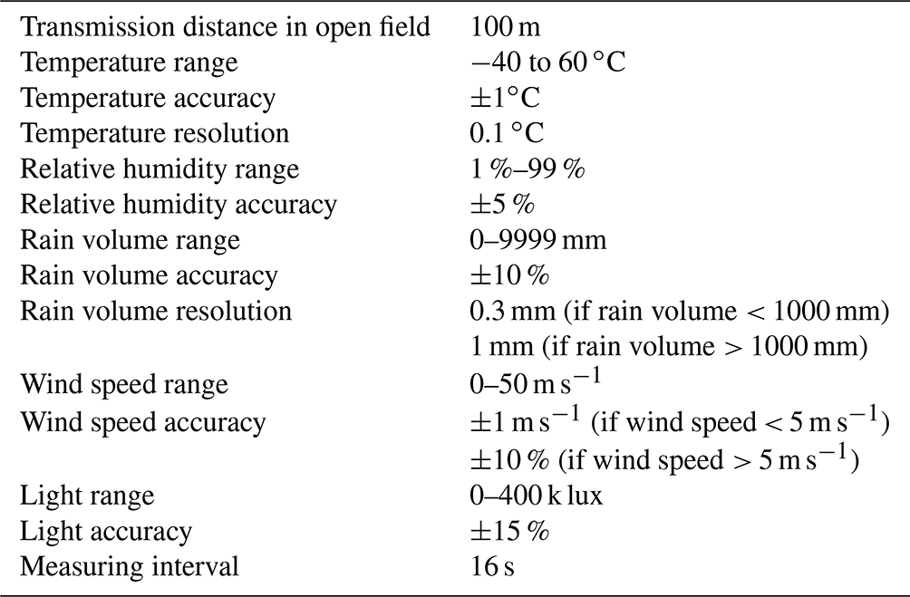
Data from the Leuven.cool citizens science network are presented in this paper. The crowdsourced weather station network consists of 106 weather stations distributed across Leuven and surroundings. The meteorological variables are measured by low-cost WH2600 wireless digital consumer weather stations produced by the manufacturer Fine Offset (Fig. 1). The station specifications, as defined by the manufacturer, are summarised in Appendix A1. The weather station consists of an outdoor unit (sensor array) and a base station. The outdoor sensor array measures temperature (in ∘C, add 273.15 for K), humidity (%), precipitation (mm), wind speed (m s−1), wind direction (∘), solar radiation (W m−2) and UV (–) every 16 s. This outdoor sensor array transmits its measurements wirelessly, via the 868 MHz radiofrequency, to the base station. This base station needs both power and internet (via a LAN connection) in order to send the data to a server. The data are forwarded to the Weather Observations Website (Kirk et al., 2020), a crowdsourcing platform initiated and managed by the UK Met Office. RMI participates in this initiative and operates its own WOW portal (Weather Observations Website – Belgium, 2022). The outdoor unit is powered by three rechargeable batteries which are recharged by a small built-in solar panel. A radiation shield protects both the temperature and humidity sensors from extreme weather conditions and direct exposure to solar radiation.

Figure 1The WH2600 wireless digital weather station outdoor unit (a) at Mathieu de Layensplein in Leuven (LC-105) and (b) next to the official AWS equipment in Humain (LC-R05) (photograph credit: Maarten Reyniers).
From July 2019 onwards, the weather stations were distributed along an urban gradient, from green (private) gardens to public grey locations, following a sampling design based on the concept of local climate zones (LCZs) (Fig. 2) (Stewart and Oke, 2012). This LCZ scheme was originally developed as an objective tool for classifying urban–rural gradients, thereby capturing important urban morphological characteristics (Verdonck et al., 2018). Stewart and Oke (2012) formally define these zones as “regions of uniform surface cover, structure, material, and human activity that span hundreds of meters to several kilometres in horizontal scale”.
Stewart and Oke (2012) define 17 LCZ classes, divided into 10 urban LCZs (1–10) and 7 natural LCZs (A–G). A LCZ map for Leuven was developed using a supervised random forest classification approach based on fine-scale land use, building height, building density and green ratio data. Details on this LCZ map are available in Appendix B. Table 2 summarises the LCZs present in Leuven and the number of weather stations in each LCZ class.
Table 2LCZs present in Leuven and the number of weather stations in each LCZ class.

It can be noted that the weather stations are not evenly distributed across the different LCZ classes, and the number of weather station within a LCZ class also does not represent the spatial coverage of this LCZ class. Due to the complex urban settings in which the network is deployed, practical limitations apply to the eligible locations for installation. We rely on citizens, private companies and government institutions giving permission to install a weather station on their property. Further, the middle-sized city of Leuven does not contain all available LCZ classes. In the urban context, compact high-rise, lightweight low-rise and heavy industry are missing. In the natural context, brush or shrub vegetation and bare soil or sand are not present in sufficiently large areas (Table 2). Furthermore, the number of stations within more natural settings is restricted due to the technical limitations of the weather stations; as previously stated, each outdoor unit needs a base station (with both power and LAN connection) within 50–100 m in order to transmit its data. Lastly, the network was implemented with the intention of gaining knowledge on the mitigating effect of green and blue infrastructures within urban settings. Thus, the weather station network mostly focusses on urban classes.
The weather stations were installed according to a strict protocol. In private gardens, the weather stations were installed at 2 m height using a steel pole with a length of 2.70 m. Dry concrete was used to anchor the pole into the soil at a depth of 70 cm. Following the station's guidelines, stations were installed in an open location within the garden, at least 1 m from interfering objects, such as nearby buildings and trees. In order to maximise the absorption of solar radiation by the solar panel and to ensure correct measurements of wind direction and precipitation, the weather station was levelled horizontally and the solar panel of the weather station was directed towards the south. Weather stations located on public impervious surfaces were installed on available light poles using specially designed L-structures to avoid direct contact with the pole. For security reasons, an installation height between 3 and 4 m was used.
The data are currently available from July 2019 (2019Q3) until December 2021 (2021Q4) (https://doi.org/10.48804/SSRN3F, Beele et al., 2022). The dataset can be downloaded in periods of 3 months and is, thus, available for each quarter. The raw 16 s measurements are aggregated (temporally averaged) to 10 min observations. This is done for three reasons: (1) an extremely high temporal resolution of 16 s is too high for most meteorological analyses, (2) the aggregation to 10 min observations is necessary to exclude the natural small-scale variability and noise in the observations, and, most importantly, (3) the reference dataset of official measurement is only available at a 10 min resolution. After resampling the data, some basic data manipulation steps are performed to obtain the correct units and resolution for every meteorological variable. The final dataset contains air temperature with the three quality level stages (see the following sections), relative humidity, dew point temperature, solar radiation, rain intensity, daily rain sum, wind direction and wind speed. We must stress that only the air temperature measurements undergo a quality check and correction procedure, as further explained in the next sections. The variables other than temperature are, however, used in the correction procedure. A qualitative assessment of the data quality of these variables is in included in Appendix C.
The maintenance of the network is controlled by PhD students and the technical staff at the Division of Forest, Nature and Landscape at KU Leuven with support from the RMI. As most of the weather stations are installed in private gardens, volunteers also keep an eye out for generic problems (e.g. leaves in the rain gauge).
Table 3Specifics of the Leuven.cool low-cost reference stations.
2.3 Reference dataset
Standard, calibrated and quality-controlled reference measurements are used to develop the QC method and evaluate its performance. As no official measurements are available in Leuven, we used data from three official RMI stations in Uccle (6447–50.80∘ N, 04.26∘ E; altitude 100 m), Diepenbeek (6477–50.92∘ N, 5.45∘ E; altitude 39 m) and Humain (6472–50.19∘ N, 5.26∘ E; altitude 295 m) (Fig. 2).
Table 4Terminology of datasets and stations used in this paper.
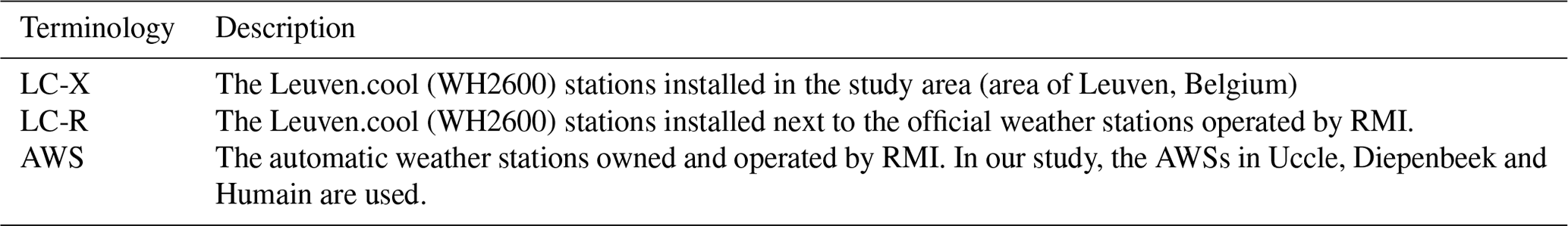
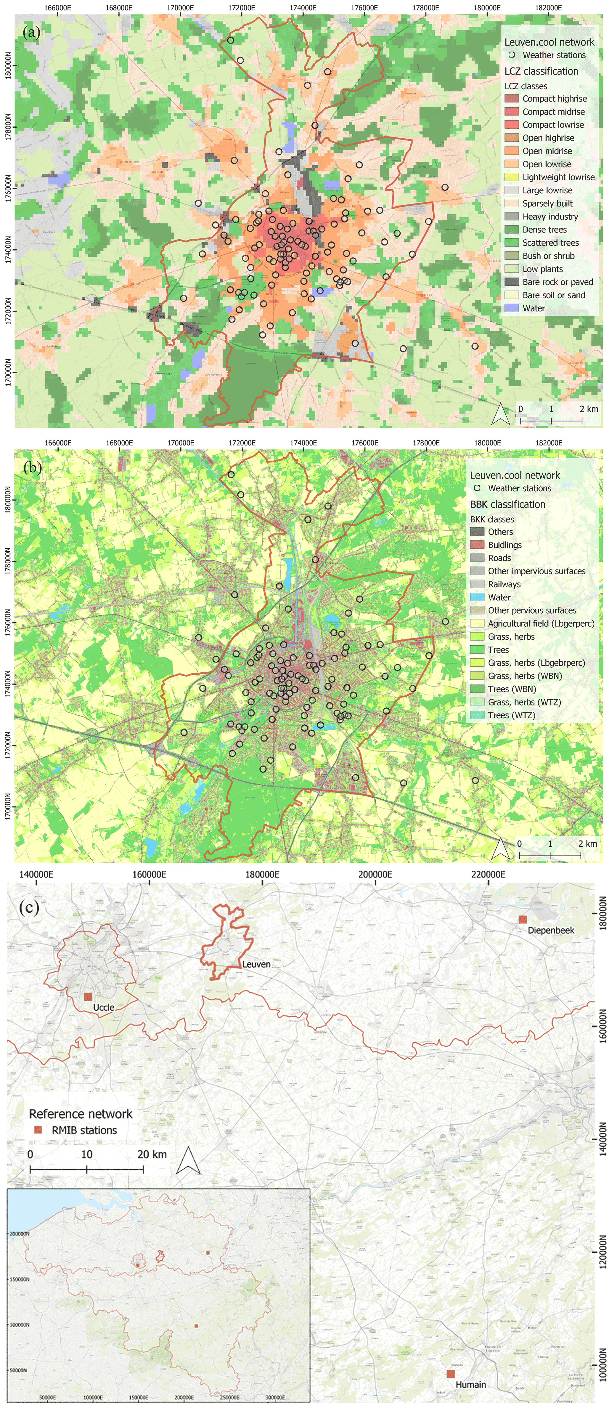
Figure 2The Leuven.cool network (LC-X) with (a) LCZ classification and (b) BBK (Bodembedekkingskaart; land use map) classification. (c) Belgium delineated by the three official regions (Flanders, Wallonia and Brussels) with the location of Leuven and the three RMI stations (AWSs) used in this study. The background map is from Esri (ESRI World Topographic Map, 2022).
The meteorological observation network of the RMI consists of 18 automatic weather stations (AWS), ensuring continuous data collection and limiting human error. These weather stations report meteorological parameters, such as air pressure, temperature, relative humidity, precipitation (quantity and duration), wind (speed, gust and direction), sunshine duration, short-wave solar radiation and infrared radiation, every 10 min. The AWS network is set up according to the World Meteorological Organization (WMO) guidelines (WMO, 2018).
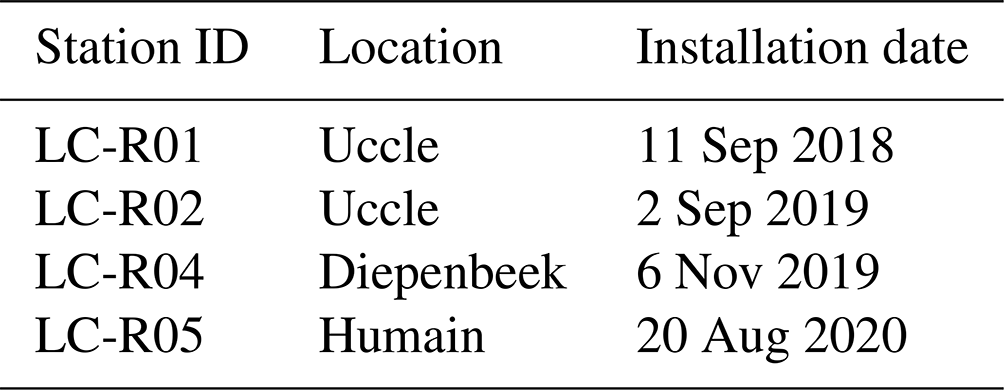
As there is no AWS available in the region of Leuven, four low-cost WH2600 weather stations were installed next to the official and more professional equipment of the RMI in Uccle, Diepenbeek and Humain. Because these stations will serve as a reference, they have been defined as LC-R01, LC-R02, LC-R04 and LC-R05 (Table 3). LC-R03 was installed for a short time in Diepenbeek, but it has been removed due to communication problems and is not taken into account in further analysis. Since January 2020, the oldest reference station LC-R01 is no longer active. This set-up enables us to calculate the temperature difference or bias between the low-cost reference stations and the official RMI stations in Uccle, Diepenbeek and Humain.
In the rest of the paper, the terminology given in Table 4 is used to refer to the different datasets and stations.
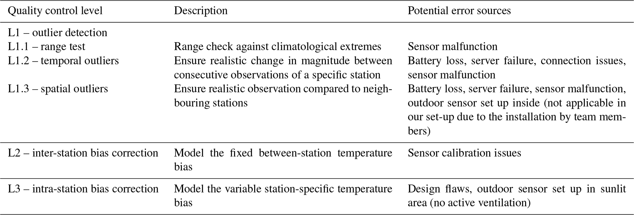
The newly developed QC control method consists of three levels (Table 5), mostly focussing on eliminating calibration issues, design flaws, and communication or software errors. Due to the strict installation protocol used for the Leuven.cool station network, some of the typical uncertainty sources are discarded a priori. Both the location and metadata of each station were controlled by experts, eliminating incomplete metadata or unsuitable installation locations. We further know that the low-cost station used in this study has some design flaws (e.g. under clear-sky and low-sun conditions, both the radiation and thermometer sensors experience shadow from the anemometer). Our correction method, however, is designed in such a way that these errors will be accounted for.
The first QC level removes implausible values mostly caused by software or communication errors. The second and third level correct for temperature biases. Both fixed inter-station (between-station) biases due to sensor calibration uncertainties and variable intra-station (station-specific) biases due to the station's design and siting are parameterised and corrected for.
Table 5Quality control levels, criteria for data filtering and potential error sources for crowdsourced air temperature measurements.
3.1 Quality control level 1 – outlier detection
The outlier detection algorithm uses a flag system in which every 10 min observation is assigned flag of 0, 1 or −1, referring to “no outlier”, “outlier” or “not enough information to determine whether observation is an outlier” respectively. The outlier detection method consists of three steps: a range test, a temporal outlier test and a spatial outlier test. The thresholds of the parameter settings used during each of these steps are explained in Table 6. We used an iterative procedure for threshold optimisation. Observations that received a flag of 1 and are, thus, defined as outliers are set to NA in the quality-controlled (QC) level 1 dataset; therefore, they are not considered during the following QC levels.

3.1.1 QC level 1.1 – range outliers
During QC L1.1, a range test based on climatology is performed. Range outliers can occur when a station is malfunctioning or is installed in an incorrect location. However, the latter has been largely eliminated by the installation protocol described in Sect. 2. Observations are flagged as 1 whenever they exceed the maxima or minima climate thresholds, plus or minus an allowed deviation ( dev). In this study, these thresholds are based on historical data from nearby official weather stations, whereas the allowed deviations from the climate thresholds are based on local knowledge on environmental phenomena. The thresholds are calculated as the maximum and minimum temperature from the official AWS in Uccle within the 3-month period that is currently undergoing QC. Observations receive a flag equal to −1 when no temperature observation is available.
3.1.2 QC level 1.2 – temporal outliers
In QC L1.2, temporal outliers are detected using both (a) a step test and (b) a persistence test. Temporal outliers occur when an observation of a specific station is not in line with the surrounding observations of this station. The step test ensures that the change in magnitude between two consecutive observations lies within a certain interval; the test checks the rate of change and flags unrealistic jumps in consecutive values. Flags are set to 1 when observations increase more than 2.5 ∘C (TOaThresMax) or decrease more than 3 ∘C (TOaThresMin) in 10 min. Such steep increases or decreases in temperature are found when a station reconnects with its receiver after a period of hitches. The values of TOaThresMin and TOaThresMax differ for meteorological reasons. The cooling down of air temperatures will, from a meteorological point of view, occur faster (e.g. through the passing of a cold front or thunderstorm) compared with the heating up of air temperatures (Ahrens, 2009). Observations are assigned a flag equal to −1 when the difference between sequential observations cannot be calculated.
The persistence test, on the other hand, makes sure that observations change minimally with time. Here, we detect stations with connection issues, such as those transmitting the same observation repeatedly. Observations changing less than 0.05 ∘C (TObThresMin) within 3 h (TObTimespan) are flagged as 1. Whenever the difference between sequential observations cannot be calculated, an observation gets a flag equal to −1.
3.1.3 QC level 1.3 – spatial outliers
QC L1.3 detects spatial outliers in the dataset. Spatial outliers occur when the observation of a specific station is too different compared with the observations from neighbouring stations. First, neighbouring stations are defined as stations located within a 2.5 km radius (range). Next, the Z score or standard score is calculated for each observation as follows:
where x is the observed value, μ is the mean value and σ is the standard deviation across all neighbours. This standard score can be explained as the number of standard deviations by which the observed value is above or below the mean value of what is being observed. Whenever the Z score is lower than −3 (SOThresMin) or higher than 3 (SOThresMax), the observation is seen as a spatial outlier and receives a flag equal to 1. When there are no neighbours available within the predefined range or the Z score cannot be calculated, each observation is flagged with −1.
3.2 Quality control level 2 – inter-station bias correction
The second quality control level corrects the data for the fixed offset or inter-station temperature bias between the weather stations. This step is necessary because the temperature sensors are only calibrated by the manufacturer, and small calibration differences are expected for this consumer-grade weather sensor. Moreover, the Leuven.cool stations originate from different production batches, with possible hardware changes in the electronics. Calibration tests between multiple LC-X stations in the same controlled environment were both technically and logistically infeasible. Simultaneous measurements are only available for two LC-R stations (LC-R01 and LC-R02 at the Uccle AWS) for a period of 4 months, showing that sensor differences indeed exist and are non-negligible. A temperature difference of 0.2 ∘C was found, which cannot be explained by the resolution of the temperature sensor (0.1 ∘C).
In order to quantify this inter-station temperature bias, a rather pragmatic approach was followed to mimic a controlled environment: we selected episodes for which a similar temperature across the study area is expected. Such episodes occur under breezy cloudy conditions with no rainfall (Arnfield, 2003; Kidder and Essenwanger, 1995). We search the database for suitable episodes every 6 months. Data are currently available from July 2019 until December 2021. As a consequence, we have looked for episodes during five 6-month periods: 2019S2 (July–December 2019), 2020S1 (January–June 2020), 2020S2 (July–December 2020), 2021S1 (January–June 2021) and 2021S2 (July–December 2021). All 10 min observations are resampled to 2 h observations, and the mean temperature, wind speed, radiation and rainfall are calculated across all weather stations. Next, suitable episodes are found by selecting episodes during which the average rainfall intensity equals 0 mm h−1 and the average radiation lies below 100 W m−2. The selected episodes are ordered by average wind speed and are limited to the top 10 results.
For these episodes, one can assume that the temperature is very uniform over the study area and is solely controlled by altitude (Aigang et al., 2009). In reality, only episodes with a high correlation between temperature and altitude (> 0.7) are retained. By regressing temperature versus altitude for every episode and calculating the residuals (i.e. the difference between the observed and predicted temperature), a fixed offset for each station and every episode is obtained. Finally, the median offset across all episodes is considered to be the true offset for each station. These offsets are subtracted from the QC level 1 temperature data in order to obtain the corrected QC level 2 temperature data.
3.3 Quality control level 3 – intra-station bias correction
During the third quality control level, the QC level 2 temperature data are further corrected for the variable intra-station temperature biases. This bias is present in the data because the measurements are made with nonstandard equipment, in contrast to the AWS measurements (e.g. passive instead of active ventilation and the dimension of the Stevenson screen). These biases change during day- and night-time as well as according to their local environment (e.g. radiation and wind speed patterns) (Bell et al., 2015).
By identifying the climatic variables mostly correlated with the temperature bias between the low-cost reference stations (LC-R stations) and the official RMI stations in Uccle, Diepenbeek and Humain (AWSs), a predictor for temperature bias is created. To produce a robust model, data from all low-cost reference stations (LC-R01, LC-R02, LC-R04 and LC-R05), ranging from their installation date until December 2021, were used simultaneously to create a predictor for the intra-station temperature bias.
For the construction of a predictor model, the dataset was randomly split in training (0.60) and validation (0.40) data. The training data were used to train simple regression models, multiple regression models, random forest (RF) models and boosted regression trees (BRTs). As previous research (Bell et al., 2015; Jenkins, 2014; Cornes et al., 2020) has shown that both radiation and wind speed highly influence the temperature bias, the simple and multiple regression models are mostly based on these variables. A previous study by Bell et al. (2015) also suggested that past radiation measurements, using an exponential weighting, are an even better prediction of the temperature bias, resulting in an advanced correction model (Bell et al., 2015). The potential predictor models are validated using the validation data, ensuring a fair evaluation of the model. The coefficient of determination (R2) and root-mean-square error (RMSE) are calculated to identify the optimal prediction model for the temperature bias. After validation, the prediction model can be applied to the weather station network in Leuven (LC-X), thereby providing a temperature bias for each observation of every station as a function of its local climatic conditions. The predicted temperature bias is subtracted from the QC level 2 temperature data to obtain the QC level 3 corrected temperature dataset.
3.3.1 The intra-station temperature bias
The overall temperature bias (i.e. all LC-R stations together) between the LC-R and the AWS data has a mean value of 0.10 ∘C and a standard deviation of 0.55 ∘C (Fig. 3). By splitting up the temperature bias for day (radiation > 0 W m−2) and night (radiation = 0 W m−2), a positive mean temperature bias during daytime (0.32 ∘C) and a negative mean temperature bias during night-time (−0.10 ∘C) is obtained. Figure 3 further suggests a higher standard deviation during daytime (0.61 ∘C) compared with night-time (0.37 ∘C), both with a remarkably skewed (and opposite) distribution.

Figure 3Histograms of the temperature bias between the low-cost reference stations (LC-R stations) and the official RMI stations (AWSs) for day and night (a), with daytime defined by radiation > 0 W m−2 (b) and night-time defined by radiation = 0 W m−2 (c). Mean biases and their standard deviations are given above the graphs. Note that the ranges on the y axis differ for the different subplots. The temperature bias was calculated for all measurements between the installation date of each LC-R and December 2021.
To get a better understanding of the monthly and daily patterns of this temperature bias, Fig. 4a shows the mean temperature bias as a function of month and hour of the day. The stations show clear diurnal and seasonal patterns, confirming the positive temperature bias during daytime and the negative temperature bias during night-time previously observed in Fig. 3. In general, we see a positive bias that is high around midday and is more pronounced during the summer months, lasting for several hours during the day. The night-time temperature bias is low for all months. A temperature bias of 0 ∘C is reached for every month at a certain time of the day; however, the specific time at which this minimal temperature bias occurs depends on the season.
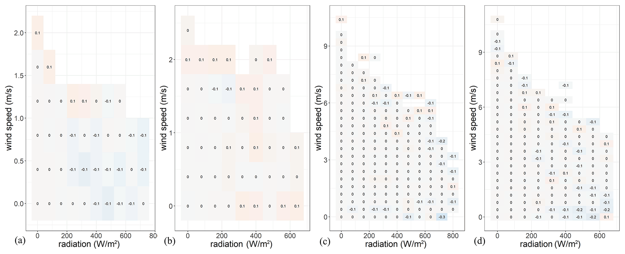
Figure 4b shows the mean temperature bias as a function of wind speed and radiation. As expected, a positive temperature bias is noticed for high-solar-radiation and low-wind-speed conditions. The rather strange high values at low radiation and high wind speed can be explained as outliers (Fig. 4c). Figure 4c shows the sample size of each cell. After removing cells with a sample size lower than 10, the final graph is obtained (Fig. 4d). The shallow local minimum seen around noon during the summer months (Fig. 4a) and the fact that the largest biases are found in the middle of the radiation range rather than at the top (Fig. 4d) are probably related to the station design itself. Two effects are at play here: (1) the placement of the radiation sensor and (2) the placement of the temperature sensor. With respect to effect (1), certainly for lower solar elevations (during winter), the wind vane casts its shadow on the radiation sensor for a short time during the day. With respect to effect (2), which we might consider more important, the temperature sensor is more shaded by the body of the station (during all seasons) around midday (highest radiation).
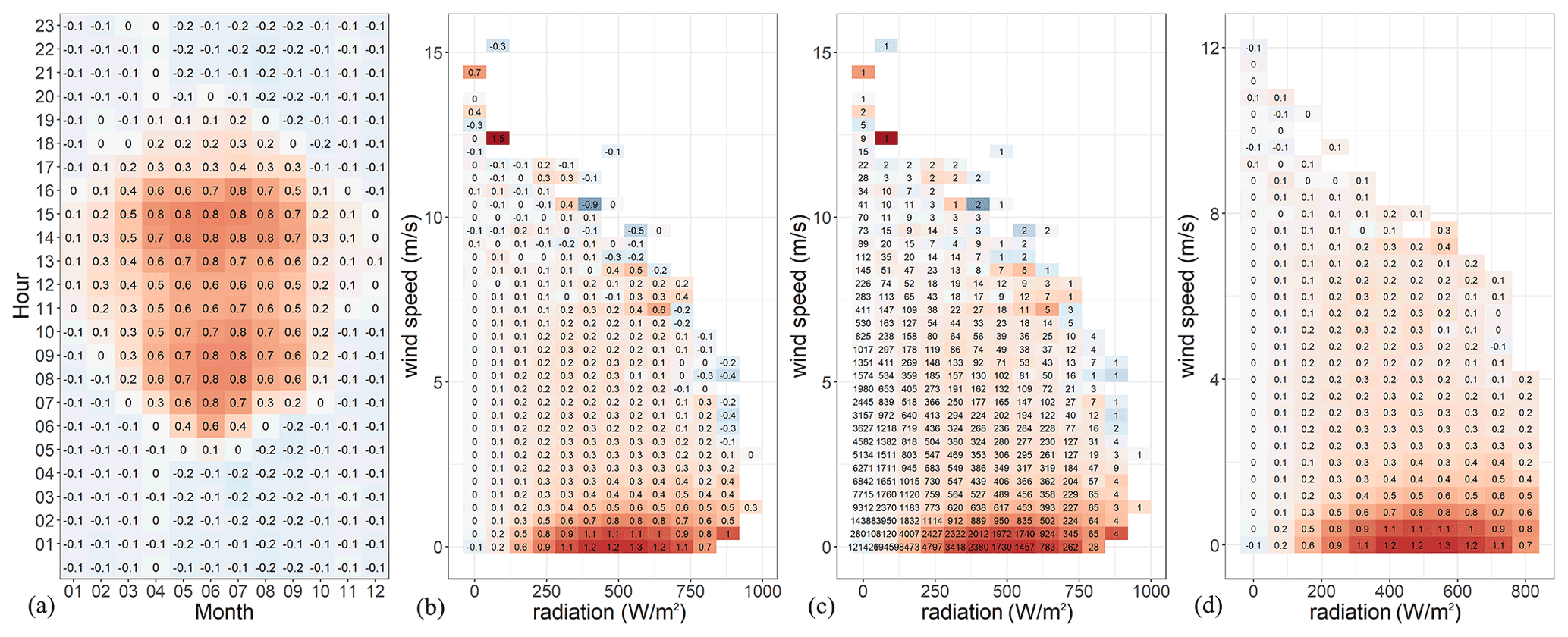
Figure 4Temperature bias (∘C) as a function of hour of the day and month of the year for all LC-R stations (a); temperature bias (∘C) as a function of radiation and wind speed for all LC-R stations (b); temperature bias (∘C) as a function of radiation and wind speed for all LC-R stations, where the values written in each cell signify the sample size (c); and temperature bias (∘C) as a function of radiation and wind speed for all LC-R stations, where cells with a sample size lower than 10 are not shown in the graph (d). Note that the ranges on the y axis differ for the different subplots. Background colours, ranging from blue (−1.7 ∘C) to red (1.7 ∘C), represent the temperature bias. The temperature bias was calculated for all measurements between the installation date of each LC-R station and December 2021.
3.3.2 Building a predictor for the intra-station temperature bias
A correlation matrix between the temperature bias and other meteorological variables, measured by the low-cost weather station, is calculated (Table 7). The values indicate how the temperature bias will change under different meteorological conditions.
Table 7The Pearson correlation matrix of temperature bias with other meteorological variables measured by the low-cost station.

The most correlated variable is radiation (0.49) directly followed by humidity (−0.48), temperature (0.41), dew point temperature (0.18) and wind speed (−0.01). As expected, taking the past radiation measurements into account further improves the correlation, reaching a maximum value when considering the last 60 min (0.56). An exponential weighting, giving higher importance to the radiation measurements closer to the temperature measurement, was used. This variable is further denoted as radiation60 (Rad60).
The variables listed in Table 7 were used to build a predictor for the temperature bias. For this purpose, multiple models were calibrated in which the temperature bias is described as a function of only one or multiple meteorological variables. In the following (Table 8 and Fig. 5), only the models with the best performance are shown. Figure 5 shows the uncorrected temperature bias (panel a) as well as the corrected temperature biases after validation with six different models: a simple linear regression with the past radiation (panel b); a multiple linear regression with the past radiation and wind speed (panel c); a multiple linear regression with the past radiation and humidity (panel d); a multiple linear regression with the past radiation, wind speed and humidity (panel e); and a random forest model (panel f) and a boosted regression trees model (panel g) including temperature, dew point temperature, humidity, radiation, radiation60, wind speed, altitude, month and hour.
Table 8The coefficient of determination (R2) and root-mean-square error (RMSE) of the different models.
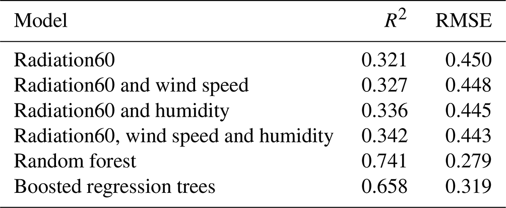
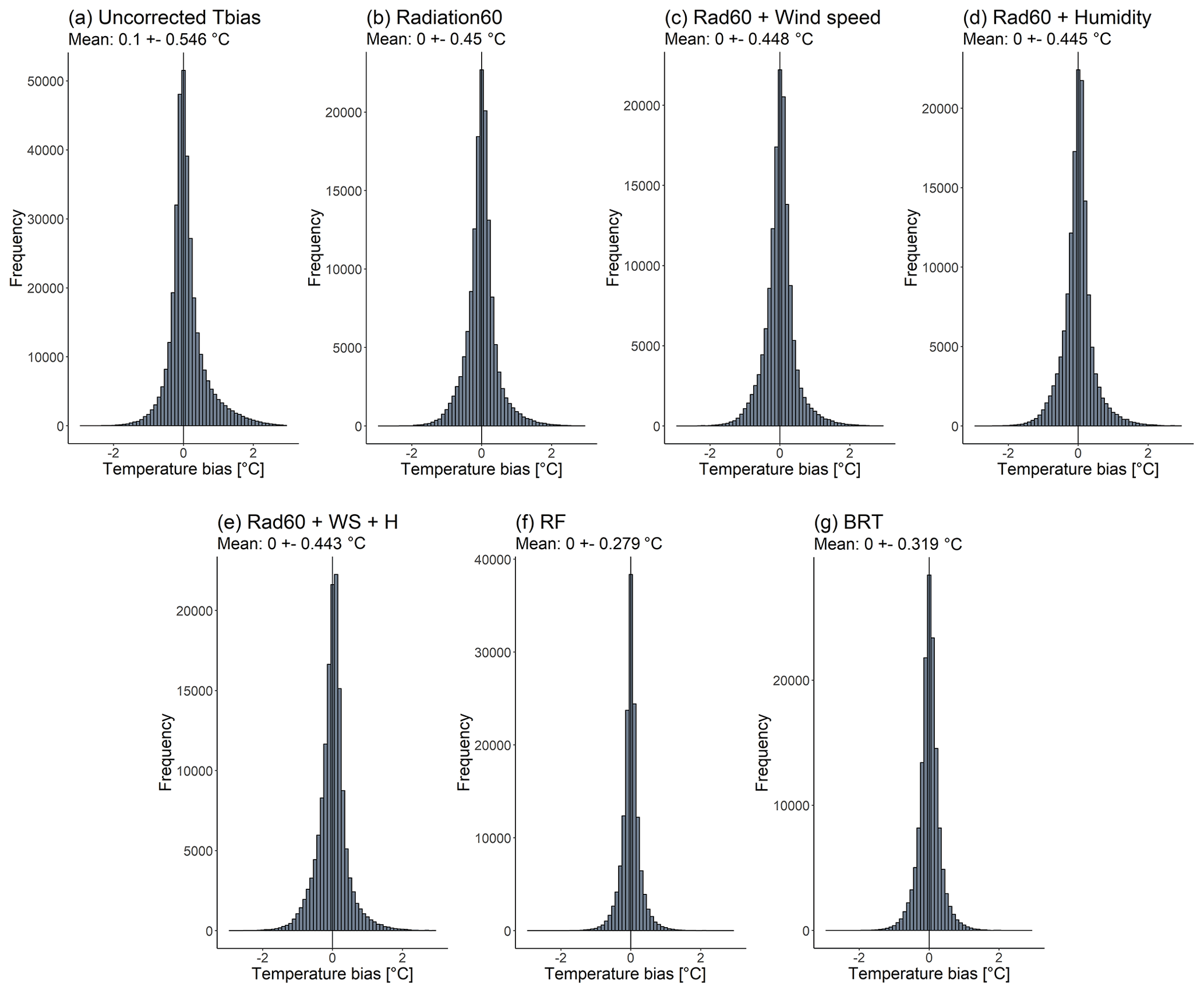
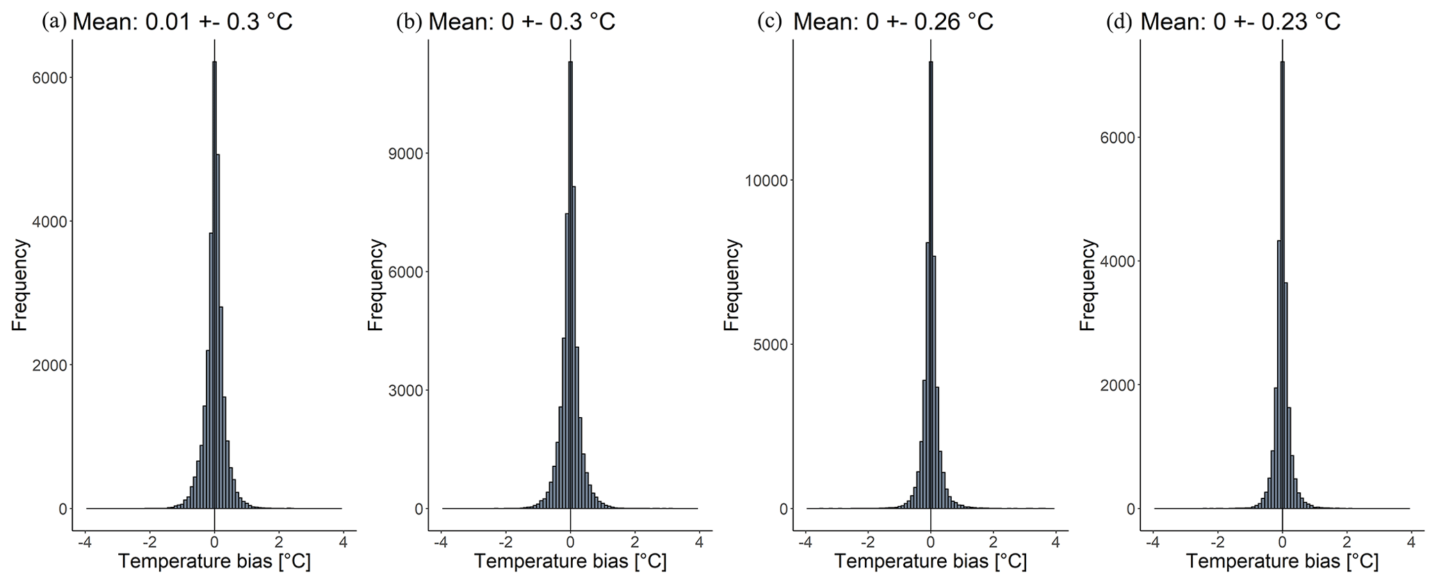
Figure 5The uncorrected temperature bias (a) and the corrected temperature bias after validation with a simple linear regression with the past radiation (b); a multiple linear regression with the past radiation and wind speed (c); a multiple linear regression with the past radiation and humidity (d); a multiple linear regression with the past radiation, humidity and wind speed (e); and a random forest model (f) and a boosted regression trees model (g) including temperature, dew point temperature, humidity, radiation, radiation60, wind speed, altitude, month and hour. Mean biases and their standard deviations are given above the graphs. Note that the ranges on the y axis differ for the different subplots.
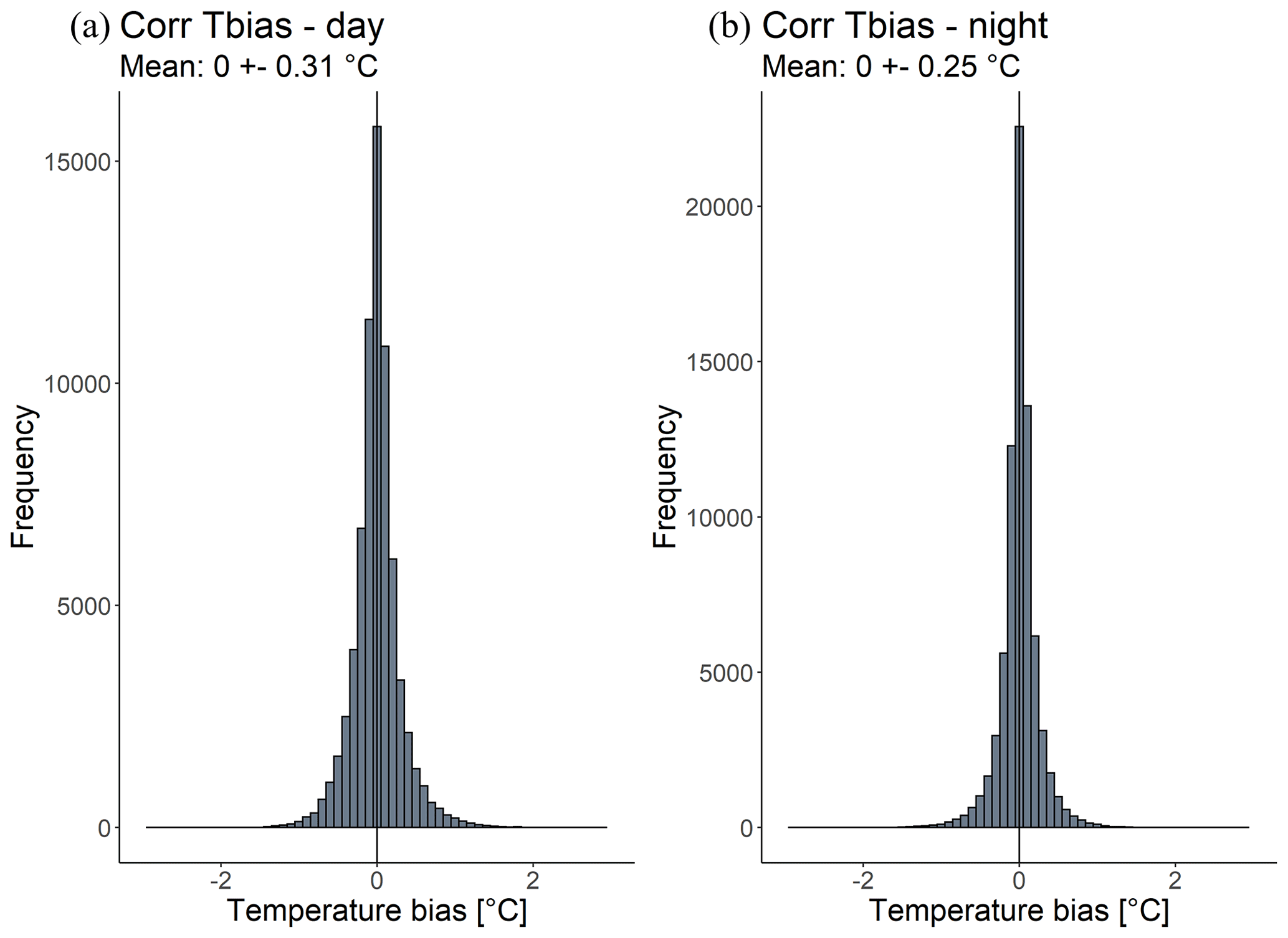
Figure 6The corrected Tbias after validation with the RF model for daytime (a) and night-time (b). Mean biases and their standard deviations are given above the graphs. Note that the ranges on the y axis differ for the different subplots.
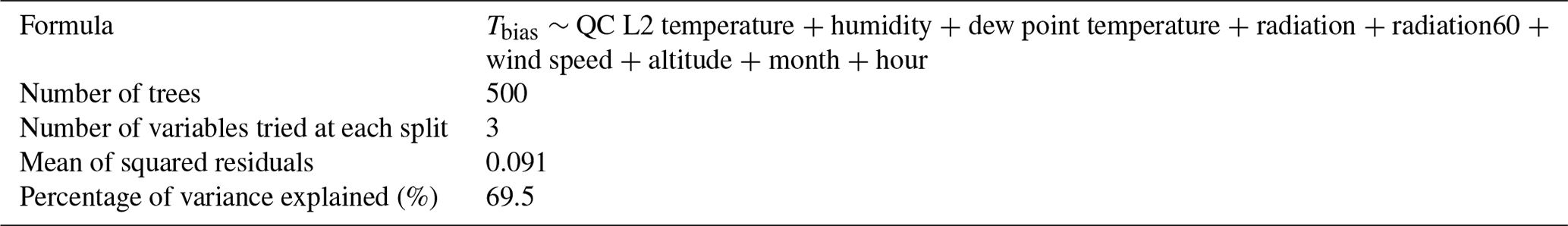
Table 9Statistical details of the RF temperature bias prediction model.
A simple linear regression based on the past radiation is already sufficient to suppress the mean temperature bias. Adding additional variables to the model, such as wind speed, humidity or both is statistically significant but only further decreases the RMSE by 0.003–0.008 ∘C. The RF and BRT models result in an RMSE of 0.279 and 0.319 and an R2 value of 0.741 and 0.658 respectively, indicating a better precision and more robust models.
The RF prediction of temperature bias showed the best results. By splitting the results up for day (radiation > 0 W m−2) and night (radiation = 0 W m−2) (Fig. 6), a smaller standard deviation of the bias during night-time (0.25) compared with daytime (0.31) is obtained. This differentiation between night and day is only for illustrative purposes; only one RF was built for both day and night. The statistical details of the RF model are further summarised in Table 9.
To evaluate the quality of the developed QC method, it is first applied to the four low-cost WH2600 stations (LC-R stations) (Table 3) installed next to the official measuring equipment in Uccle, Diepenbeek and Humain (AWSs). Comparing this LC-R dataset with the AWS dataset allows us to investigate the improvement or deterioration of the data quality after each QC level.
4.1 Quality control level 1 – outlier detection
For QC L1.1, the range outliers are detected by comparing the temperature of each LC-R station with the climatic thresholds set by its nearby official AWS ( dev_reference). As can be seen from Table 6, the deviation allowed from the climatic thresholds is smaller for the LC-R stations compared with the LC-X stations in the study area. This is due to the fact that the LC-R stations are installed next to the official AWSs; thus, no environmental factors should be taken into account. The temporal outliers are detected in QC L1.2 by comparing the rate of change between consecutive observations with the thresholds defined in Table 6. In QC L1.3, spatial outliers are detected using the Z score. We should, however, stress that this analysis is not ideal because every reference station only has one neighbour – the official AWS station. Only LC-R01 and LC-R02, located in Uccle, have two neighbours during a period of 4 months, when both stations were active simultaneously.
The results show no spatial outliers for the LC-R stations. Some observations are, however, highlighted as range or temporal outliers. Table 10 summarises the number and percentage of observations flagged as 1. These observations are set to NA, resulting in the temperature dataset with quality level 1. The temperature profiles of the LC-R stations versus the official AWS temperature (Fig. 7; solid versus dashed grey line) highlight observations defined as range or temporal outliers using circles or squares respectively. Scatterplots in which the temperature of the LC-R stations is compared to the temperature of the AWSs (Fig. 8) use the same layout. The temperature difference between the LC-R stations and the AWSs () is calculated as an effective quality measure.
Table 10Number and percentage of observations flagged as outliers during QC level 1.
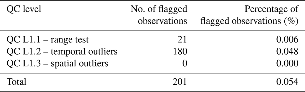
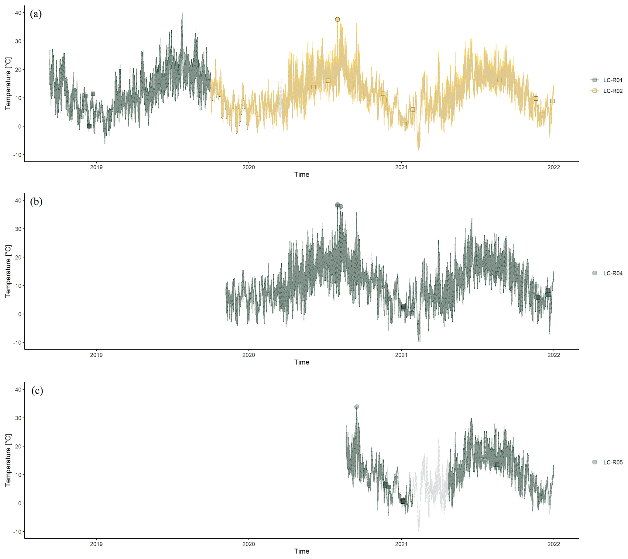
Figure 7Temperature profile of LC-R stations in (a) Uccle (LC-R01 and LC-R02), (b) Diepenbeek (LC-R04) and (c) Humain (LC-R05). The grey dashed line represents the official AWS temperature of a specific location. Observations defined as range outliers are symbolised by a circle, and temporal outliers are symbolised by a square. The temperature profiles include all measurements between the installation date of each LC-R and December 2021.
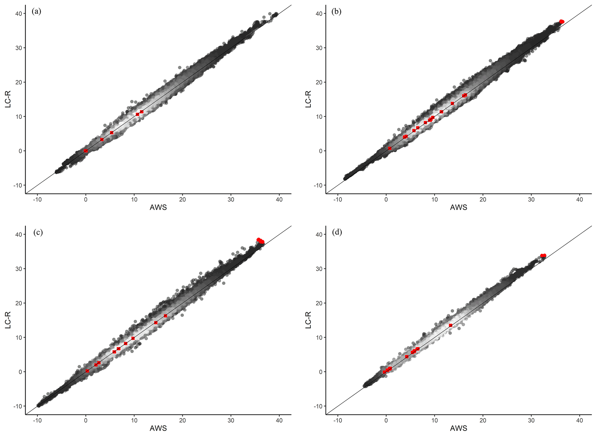
Figure 8Scatterplots of LC-R versus AWS temperature for each reference station, (a) LC-R01, (b) LC-R02, (c) LC-R04 and (d) LC-R05, at QC level 0. Observations defined as range outliers are symbolised by a red circle, and temporal outliers are symbolised by a red square. The identity line is shown in black. The colour scale indicates the density of observations, with white indicating the highest and black indicating the lowest. The scatterplots include all measurements between the installation date of each LC-R and December 2021.
The results show only a few range outlier and even no spatial outliers for the LC-R stations. The procedure does, however, highlight 180 observations as temporal outliers (Table 10). These observations were highlighted during the persistence test: 180 observations change less than 0.05 ∘C within 2 h. With only 0.054 % of the observations flagged as outliers, we can conclude that the LC-R dataset does not contain a lot of outliers. Because of their importance in this QC method, especially in QC L3, these reference stations are indeed closely monitored, thereby preventing and minimising the occurrence of outliers. As only 0.054 % of the data were set to NA, no difference in the ΔT statistics occurred. Thus, the histograms in Fig. 9 represent the data with both QC level 0 and QC level 1. The mean temperature difference ± standard deviation for all reference stations is 0.15 ± 0.56 ∘C.
Reference station LC-R01 only has a small positive mean ΔT, whereas the mean ΔT values of LC-R02 and especially LC-R05 are remarkably higher. The mean ΔT of LC-R04 equals zero. The standard deviations of LC-R04 and L-R05 are noticeably smaller than those of LC-R01 and LC-R02 (Fig. 9). As expected, the temperature difference between the LC-R stations and the AWSs is not constant and is correlated with other variables. A higher difference is obtained during the summer months (Fig. 10) under low-cloud and low-wind-speed conditions (Fig. 11).

Figure 9Histograms of temperature difference () for each reference station, (a) LC-R01, (b) LC-R02, (c) LC-R04 (d) and LC-R05, at QC level 0 and QC level 1. The mean differences and their standard deviations are given above the graphs. Note that the ranges on the y axis differ for the different subplots. The temperature difference was calculated for all measurements between the installation date of each LC-R and December 2021.

Figure 10Temperature difference () as a function of hour of the day and month of the year for each reference station, (a) LC-R01, (b) LC-R02, (c) LC-R04 and (d) LC-R05, at QC level 1. Background colours, ranging from blue (−1.7 ∘C) to red (1.7 ∘C), represent the ΔT. The temperature difference was calculated for all measurements between the installation date of each LC-R and December 2021.
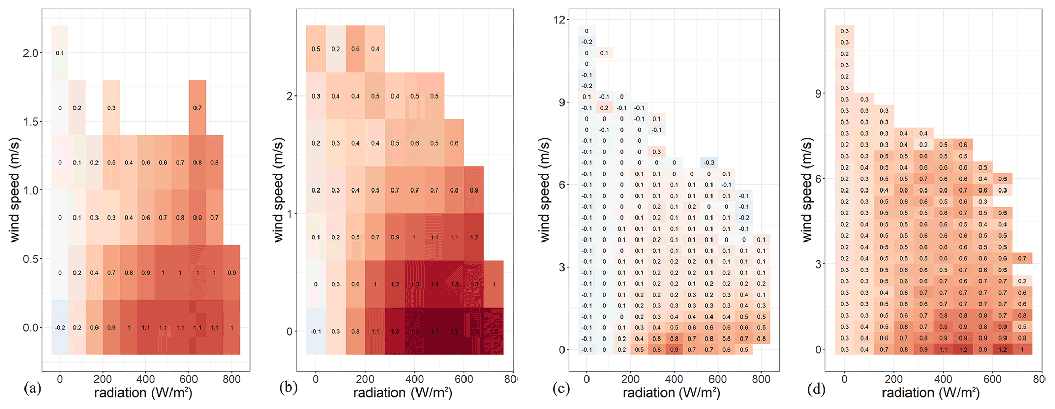
Figure 11Temperature difference () as a function of radiation and wind speed for each reference station, (a) LC-R01, (b) LC-R02, (c) LC-R04 and (d) LC-R05, at QC level 1. Cells with a sample size lower than 10 are not shown in the graph. Note that the ranges on the y axis differ for the different subplots. Background colours, ranging from blue (−1.7 ∘C) to red (1.7 ∘C), represent the ΔT. The temperature difference was calculated for all measurements between the installation date of each LC-R and December 2021.

Figure 12Offsets during the selected episodes (dots), showing the median offset (diamond) and its error bar (mean ± standard deviation) for each reference station (LC-R). For reference, the zero line is plotted in red.
4.2 Quality control level 2 – inter-station bias correction
During QC level 2, temperatures are corrected for the fixed offset between stations or the inter-station bias, due to intrinsic sensor differences at the level of the electronics. The proposed methodology of searching for episodes with a very uniform temperature field over the study area (see Sect. 3) cannot be applied here due to the large distance between the three locations with LC-R stations.
Here, we selected episodes for which we expect a similar temperature between the LC-R stations and the AWSs. This occurs again under breezy cloudy conditions with no rainfall (Fig. 11). For each reference station, all 10 min observations are resampled to 2 h observations, and the mean temperature, wind speed, radiation and rainfall are calculated. Next, suitable episodes are found by selecting episodes in which the average rainfall intensity equals 0 mm h−1 and the average radiation lies below 100 W m−2. The selected episodes are ordered by average wind speed and are limited to the top 10 results. The mean LC-R and AWS temperature is calculated for each episode, and an offset between both is then calculated. Finally, the median offset across all episodes is considered to be the true offset for each station. These offsets are subtracted from the QC L1 temperature data in order to obtain a corrected temperature: the QC level 2 dataset.
Reference stations LC-R01 and LC-R04 have a small negative offset, equal to −0.029 and −0.072 ∘C respectively. Stations LC-R02 and LC-R05 have positive and notably larger offsets, equal to 0.113 and 0.243 ∘C respectively (Fig. 12).
To check the quality improvement of QC level 2, the temperature difference () between the LC-R stations and the AWSs is again calculated for every station (Fig. 13). Reference stations LC-R01 and LC-R04 show a small increase in their mean ΔT; however, the mean ΔT of LC-R02 and LC-R05 decreases. As a result, the ΔT of all stations becomes more equal. As QC level 2 only added a fixed temperature offset, the standard deviations of all ΔT values remain the same. The inter-station bias correction further highlights the seasonal and daily pattern of the ΔT, especially for reference station LC-R05 (Fig. 14).

4.3 Quality control level 3 – intra-station bias correction
From Sect. 3, we recall that the random forest prediction of temperature bias showed the best results After applying this prediction model on the reference dataset (LC-R), a level 3 corrected temperature is obtained for each LC-R station. These results could be biased because the RF model is trained on 60 % of the LC-R dataset and then applied to the complete LC-R dataset. To account for this, we applied the prediction model to both the complete dataset and the test dataset (which was not used for training the model). The outcome for each LC-R is listed in Appendix D. It can be noted that mean T difference remains equal for both datasets, and the standard deviation does slightly increase by 0.5 to 0.7 ∘C when using the test dataset. The results below are based on the test dataset only.
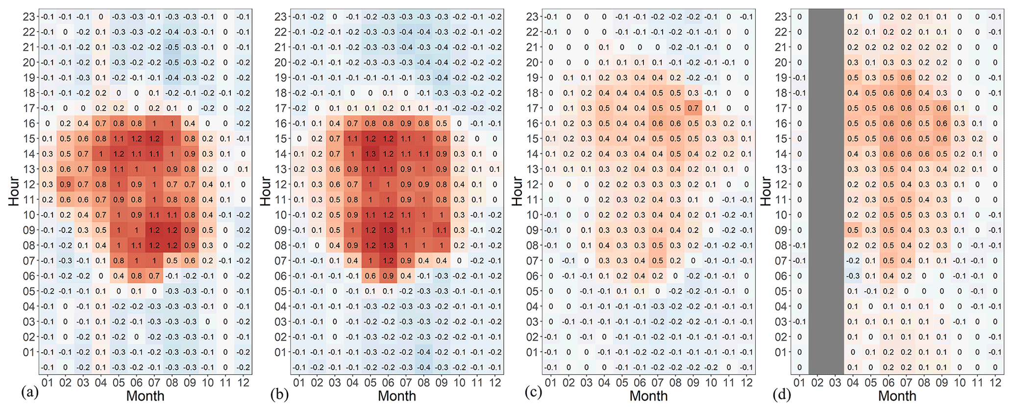
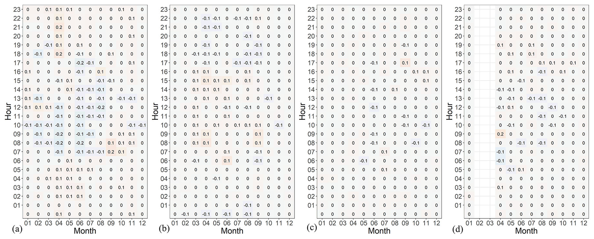
To evaluate the quality improvement of QC level 3, the temperature difference () between the LC-R stations and the AWSs is again calculated for every station (Fig. 15). Histograms of the temperature show a mean ΔT of almost 0 ∘C for each reference station, and the standard deviation clearly decreased compared with QC level 2 (Fig. 13). When the ΔT is plotted as a function of each month and hour of the day, one can notice that the diurnal and seasonal pattern is completely corrected for (Fig. 16). Moreover, the effects of wind speed and radiation are effectively eliminated (Fig. 17). The mean temperature difference ± standard deviation for all LC-R stations is 0.00 ± 0.28 ∘C.
In this section, the newly developed QC method is applied to the low-cost stations of the Leuven.cool network (LC-X). The Leuven.cool dataset currently ranges from July 2019 (2019Q3) until December 2021 (2021Q4). The QC method is performed four times per year, each time for a period of 3 months.
5.1 Quality control level 1 – outlier detection
During QC level 1, range, temporal and spatial outliers are removed using climatological thresholds from Uccle, neighbouring observations (i.e. circumjacent/surrounding observations from the same station) and neighbouring stations (i.e. simultaneous observations from neighbouring stations) respectively. If no official weather station is available, thresholds can be based on existing climate classification maps. Table 11 summarises the number of observations flagged as outliers in each step. For each year, only between 0.5 % and 1 % of the data are defined as outliers and thus eliminated, indicating that the raw data quality is rather good compared with other citizens science networks.
Table 11Number and percentage of observations flagged as outliers during QC level 1 for 2019 Q3–Q4, 2020 Q1–Q4 and 2021 Q1–Q4 for all LC-X measurements.
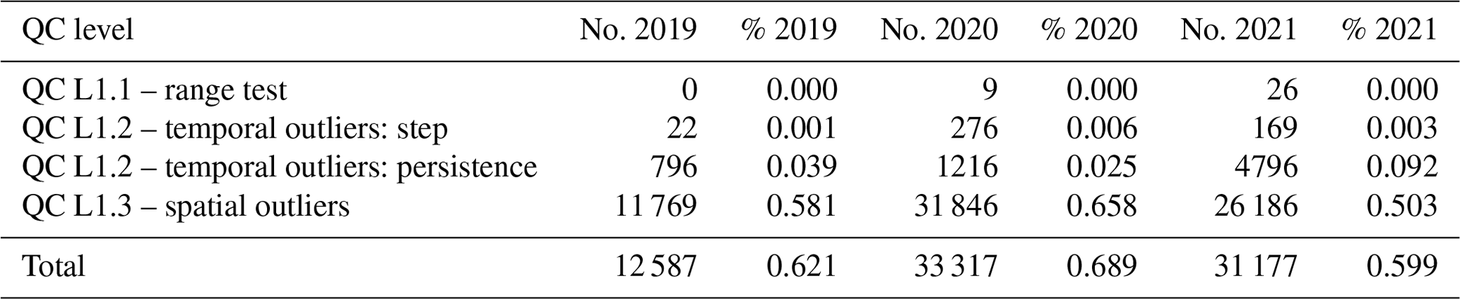
The simple spatial outliers test performed by Chapman et al. (2017) yielded comparable results: 1.5 % of the data were omitted in this study. Other studies have reported a much higher fraction of eliminated data: Meier et al. (2017) only kept 47 % of the raw data after conducting their four-step QC analysis, and Napoly et al. (2018) and Feichtinger et al. (2020) kept 58 % and 55 % of the data respectively. CrowdQC+, as a further development of CrowdQC, results in an even lower data availability: only 30 % of the raw data remain after the QC (Fenner et al., 2021). These high numbers of omitted data can, however, be explained by (1) a great number of CWSs being installed indoors (not applicable in our set-up) and, thus, lacking the typical diurnal temperature patterns, and (2) radiative errors due to solar radiation exposure of poorly designed devices, resulting in very high temperature observations (Napoly et al., 2018; Fenner et al., 2021). In the QC method presented in this paper, calibration and radiative errors are, however, corrected for during QC level 2 and 3, rather than being omitted.
5.2 Quality control level 2 – inter-station bias correction
In QC level 2, a fixed offset for each weather station is obtained. These offsets, induced by the intrinsic differences in the level of the sensors' electronics, are subtracted from the station's temperature, thereby accounting for calibration errors. The obtained offsets, the median offset and its error bar (mean ± standard deviation) are plotted in Fig. 18 for each station. The mean offset of all stations equals 0.010 ∘C. Station LC-102 has the highest offset (0.349 ∘C), whereas station LC-074 has the lowest offset (−0.220 ∘C). It can be noticed that the error bars of most stations are rather small, which reinforces our confidence in a valid determination of the fixed calibration offset.
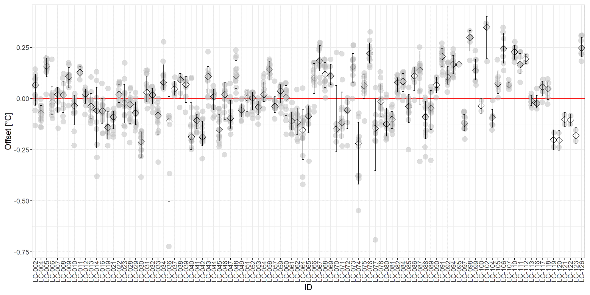
Figure 18Offsets during the selected episodes (grey dots), the median offset (black diamond) and its error bar (mean ± standard deviation) for each LC-X station active during at least one episode. For reference, the zero line is plotted in red.
For stations that were not active during one of the selected timeframes, we were not able to determine their calibration offset (stations LC-003, LC-096, LC-108, LC-109, LC-114, LC-124, LC-125, LC-127 and LC-128). As a consequence, no corrected temperature could be calculated, meaning that those stations are not considered during the following QC level (QC level 3). The search for episodes should be extended with upcoming periods of 6 months in order to resolve this problem.
5.3 Quality control level 3 – intra-station bias correction
In QC level 3, the random forest model is applied to each temperature observation of all LC-X stations in order to obtain a site- and time-specific prediction of its temperature bias. As expected, this prediction shows the same pattern as seen for the LC-R stations: generally, we see a positive bias that peaks around midday and is more pronounced during both summer months and low-cloud and low-wind-speed conditions (Fig. 19). Note that the actual bias calculation in QC level 3 is performed for every timestamp and every LC-X station separately using the other weather variables measured by the station, as input for the RF model. After subtracting this temperature bias from the observed temperature, the corrected temperature for each station is obtained.

Figure 19(a) Prediction of the temperature bias (∘C) as a function of hour of the day and month of the year for all LC-X stations and (b) prediction of the temperature bias (∘C) as a function of radiation and wind speed for all LC-X stations, although cells with a sample size lower than 10 are not shown in the latter graph. Background colours, ranging from blue (−1.7 ∘C) to red (1.7 ∘C), represent the temperature bias. The prediction of the temperature bias was calculated for all LC-X measurements from July 2019 to December 2021.
These results are in line with the findings of Jenkins (2014) and Bell et al. (2015): both found a significant positive instrument temperature bias during daytime with a strong relation to the incoming solar radiation for multiple types of crowdsourced weather stations. To our knowledge, prior to our study, only Cornes et al. (2020) had used the findings of Bell et al. (2015) to actually correct crowdsourced air temperature data. Radiation from satellite imagery and background temperature data from official stations were used to parameterise the short-wave radiation bias; as a consequence, no correction was performed for night-time. The data correction has reduced the error from ±0.2–0.8 to ±0.2–0.4 ∘C. These results are comparable with our results, although slightly smaller errors of only ±0.23–0.30 ∘C are obtained here (Fig. 15). Cornes et al. (2020) did suggest the incorporation of wind speed as an additional covariate in order to incorporate the effect of passive ventilation. The random forest model described in this study does include additional covariates, including wind speed, but most importantly only needs data from the weather station itself. No satellite imagery nor official stations are needed once the random forest model is built. Cornes et al. (2020) further highlighted the need for station-specific quality controls in order to remove the confounding effect of different instrument types. With the use of a unique station type, we aimed at minimising such effects in our dataset. QC level 2 (Sect. 5.2) showed that these effects were indeed limited.
5.4 Overall impact of the QC method on the dataset
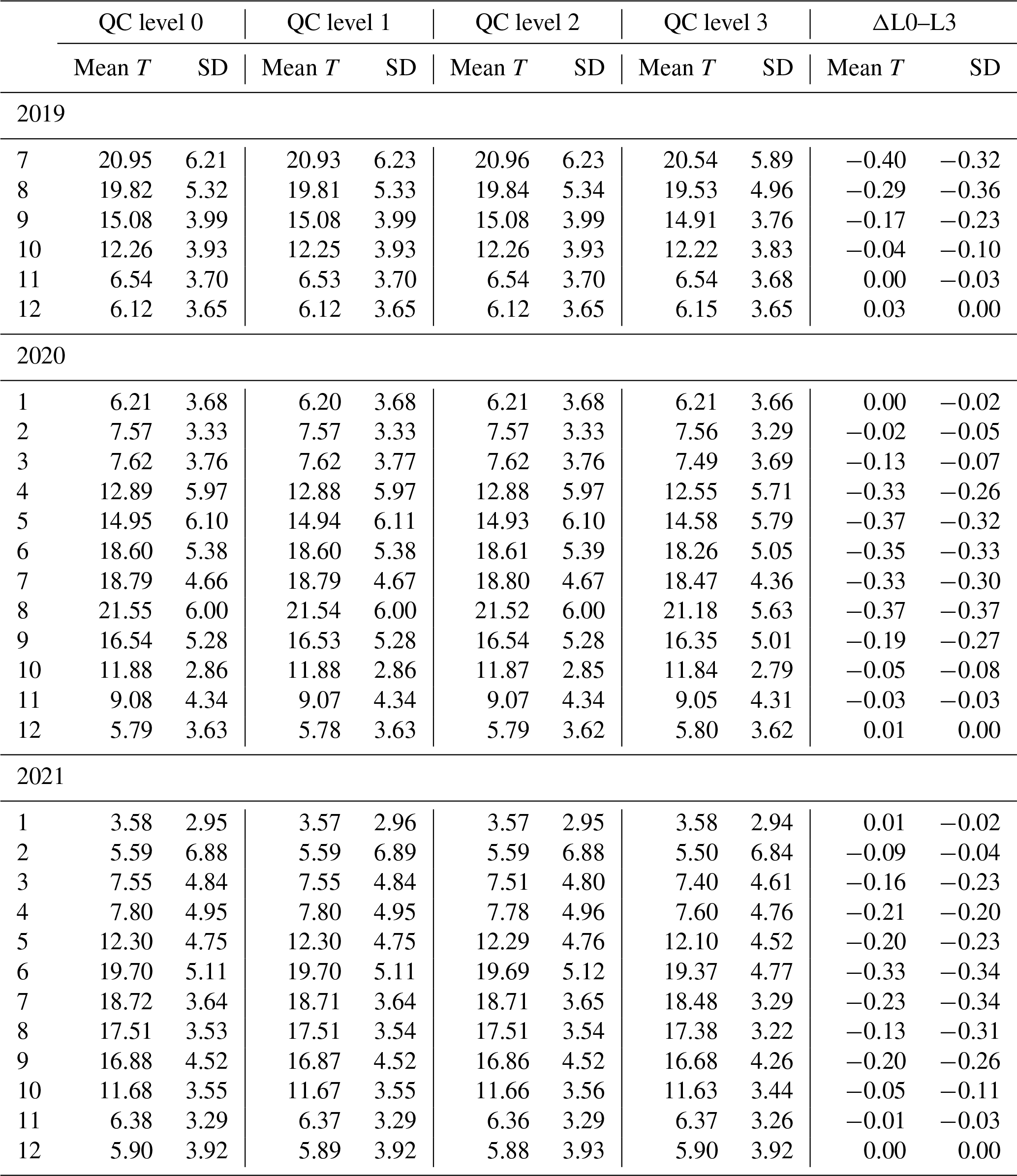
To assess the impact of the different QC stages on the global dataset, several violin boxplots were created on both a monthly and yearly base. Figure 20 illustrates the monthly violin plots for 2019, 2020 and 2021 at each quality control level. Table 12 summarises the mean monthly temperature and its standard deviation for each quality control level.
The violin plots and the accompanying mean temperature and standard deviation do not change much over the different QC levels. As QC level 1 removes outliers from the dataset, we would expect a lower standard deviation for QC level 1 compared with QC level 0. Figure 20 does indicate the removal of some outliers, but Table 12 does not confirm the expected decrease in the standard deviation. This can be explained by the low percentage of observations defined as outliers: for each year, only 0.5 % to 1 % of the data were defined as outlier. Due to the strict installation protocol, most errors were already eliminated upfront. If errors do occur as the result of a station malfunction, they are quickly resolved because the dataflow and station siting are continuously controlled.
During QC level 2, each station is corrected for its inter-station temperature bias. As both positive and negative biases, ranging from 0.349 to −0.220 ∘C, are possible, no clear change in the mean temperature is expected between QC level 1 and QC level 2. Because this QC level corrects each station with a fixed offset, the standard deviation should stay the same. Both of these assumptions are confirmed by Fig. 20 and Table 12.
During the QC level 3, we do see a clear change in mean temperature and standard deviation. For the summer months, a reduction in the mean temperature and standard deviation of up to −0.40 and −0.36 ∘C is noted respectively. The change in the standard deviation shows a monthly pattern with a higher reduction during the summer months and almost no change during winter. The change in mean temperature is not as consistent and seems dependent on the observed temperatures. A higher reduction in mean temperature is noted for the hot summers of 2019 and 2020 compared with the rather cold summer of 2021. These results can easily be explained by the daily and seasonal patterns of the predicted temperature bias (Fig. 19).
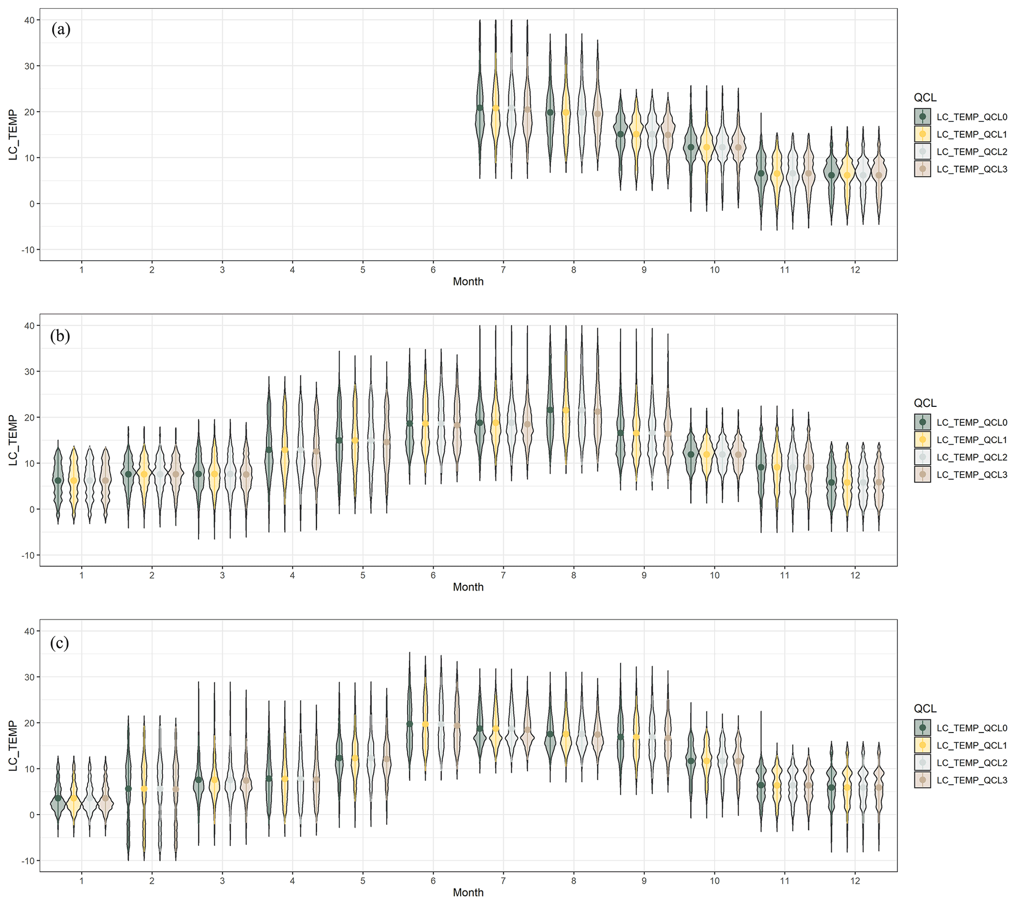
Figure 20Monthly violin plots of temperature data (∘C) of all LC-X stations at quality control level 0 (raw data), level 1 (outliers removed), level 2 (inter-station bias correction) and level 3 (intra-station bias correction) for 2019 Q3–Q4 (a), 2020 Q1–Q4 (b) and 2021 Q1–Q4 (c).
Table 12The mean monthly temperature (∘C) and its standard deviation (SD) for all LC-X stations at quality control level 0 (raw data), level 1 (outliers removed), level 2 (inter-station bias correction) and level 3 (intra-station bias correction).
A validation of the proposed QC method showed that it can reduce the mean temperature difference and standard deviation from 0.15 ± 0.56 to 0.00 ± 0.28 ∘C. The QC method can correct the temperature difference equally across different hours of the day and months of the year (Fig. 16) as well as under different radiation and wind speed conditions (Fig. 17).
The quality-controlled Leuven.cool dataset enables a detailed comparison with other crowdsourced datasets for which less or even no metadata are available. As such, the Leuven.cool stations can serve as gatekeepers for other crowdsourced observations. In the past, this role has been limited to standard weather station networks which mostly only have a limited number of observations available (Chapman et al., 2017).
Numerous studies have shown that the UHI effect causes night-time temperature differences of up 6 to 9 ∘C during clear nights (Chapman et al., 2017; Venter et al., 2021; Stewart, 2011; Napoly et al., 2018; Feichtinger et al., 2020). These thresholds are much higher than the mean bias obtained after correction. Thus, the dense quality-controlled Leuven.cool dataset allows for microscale modelling of urban weather patterns, including the UHI (Chapman et al., 2017; de Vos et al., 2020; Napoly et al., 2018; Feichtinger et al., 2020). As such high-quality datasets contain measurements with both high spatial and temporal resolution, they can easily be used to obtain spatially continuous temperature patterns across a region (e.g. Napoly et al., 2018; Feichtinger et al., 2020). Interpolation methods based on single pairs of stations or mobile transect methods are much less trustworthy (Napoly et al., 2018). Dense weather station networks can be used to investigate the inter- and intra-LCZ variability within a city (Fenner et al., 2017; Verdonck et al., 2018). The dataset can further help investigate the relation between temperature and human and ecosystem health (e.g. Demoury et al., 2022; De Troeyer et al., 2020) as well as their effect on evolutionary processes (e.g. Brans et al., 2022).
The dataset can also help refine existing weather forecast models which are currently mostly based on official rural observations (Sgoff et al., 2022). Nipen et al. (2020) showed that the inclusion of citizen observations improves the accuracy of short-term temperature forecasts in regions where official stations are sparse. Mandement and Caumont (2020) used crowdsourced weather stations to improve the observation and prediction of convection patterns near the ground. After quality control and correction, the wind (Chen et al., 2021) and precipitation measurements (de Vos et al., 2019) can also be useful to improve detection and forecasting. Further, the Leuven.cool dataset could be a useful input in air pollution prediction models (e.g. Immission Frequency Distribution, IFD, model, Lefebvre et al., 2011).
All data described in this paper and the scripts used to design, evaluate and apply the QC method are stored in RDR, the KU Leuven Research Data Repository, and are accessible via the following DOI: https://doi.org/10.48804/SSRN3F (Beele et al., 2022). The dataset is accompanied by an extensive README file explaining the content of the dataset. The dataset includes a metadata file (01_Metadata.csv), the actual observations for every 3 months/quarter (LC_YYYYQX.csv), and the R scripts needed to build and apply the QC method (LC-R_QCL1-2-3.Rmd and LC-X_QCL1-2-3.Rmd). The metadata file contains information on weather station coordinates, altitude above sea level, installation height, LCZ class, dominant land cover, mean sky view factor (SVF) and mean building height in a buffer of 10 m around each weather station. Coordinates have been rounded to three significant figures for privacy reasons. The actual observations are given as 10 min aggregates and include relative humidity [%], dew point temperature [∘C], number of 16 s observations in 10 min aggregate, solar radiation [W m−2], rain intensity [mm h−1], daily rain sum [mm], wind direction [∘], wind speed [m s−1], date [YYYY-MM-DD], year [YYYY], month [MM], day [DD], hour [HH], minute [MM], weighted radiation during last the 60 min [W m−2], temperature at QC level 0 [∘C], temperature at QC level 1 [∘C], temperature at QC level 2 [∘C] and temperature at QC level 3 [∘C].
This study presents the data from the citizen science weather station network Leuven.cool, which consists of around 100 weather stations in the city of Leuven, Belgium. The crowdsourced weather stations (Fine Offset WH2600) are distributed across Leuven and surroundings, and they have been measuring the local climate since July 2019. The dataset is accompanied by a newly developed station-specific temperature quality control procedure. The quality control method consists of three levels that remove implausible measurements while also correcting for inter-station (between-station) and intra-station (station-specific) temperature biases. This QC method combines the suggestions of previously developed methods but improves them by correcting aberrant temperature observations rather than removing them. As a result, more data can be retained, allowing researchers to study the highly heterogeneous urban climate in all its detail. Moreover, the QC method uses information from the crowdsourced data itself and only requires reference data from official stations during its development and evaluation stage. Afterwards, the method can be applied independently of the official network that was used in the development phase. Transferring the method to other networks or regions would require the recalibration of the QC parameters. Specifically, for QC L1.1, some indication of climate thresholds is needed. QC L1.3 and QC L2 require a dense weather station network; thus, the QC method is less suitable for single or few stations. For QC L3, a large amount of other data (e.g. radiation and wind speed) are needed. The random forest model is, however, easily adaptable to the parameters that are available.
A validation of the proposed QC method was carried out on four Leuven.cool stations installed next to official equipment, and it showed that the QC method is able to reduce the mean temperature difference ± standard deviation from 0.15 ± 0.56 to 0.00 ± 0.28 ∘C. The quality-controlled Leuven.cool dataset enables a detailed comparison with other crowdsourced datasets for which less or even no metadata is available. The dense dataset further allows for microscale modelling of urban weather patterns, such as the UHI, and can help identify the relation between temperature and human and ecosystem health as well as their effect on evolutionary processes. Lastly, the dataset could be used to refine existing forecast models, which are currently mostly based on official rural observations. Knowing that both the frequency and intensity of heat waves will only increase during the upcoming years, dense high-quality datasets such as Leuven.cool will become highly valuable for studying local climate phenomena, planning efficient mitigation and adaptation measures, and mitigating future risks.
The technical specifications of the Fine Offset WH2600 weather station are given in Table A1.
Table A1Technical specifications of the Fine Offset WH2600 weather station, as given by the manufacturer.
The LCZ map was created using a supervised random forest classification approach based on fine-scale land use, building height, building density and green ratio data within R. The input data used for the creation of the LCZ map are listed in Table B1. All input datasets were rasterised and cropped to a spatial resolution of 100 m.
A 15 km × 15 km grid area was drawn around the city centre of Leuven. Within this grid area, training polygons for 12 LCZ types (7 urban LCZs and 5 natural LCZs) were drawn. The delineation of the urban training areas was based on the same input data layers. The threshold values used during this process are further described in Fig. B1. The training areas are plotted in Fig. B2.
The training polygons were randomly split in training (0.7) and validation (0.3) data. Subsequently, a random forest model was trained and validated using both datasets. A majority filter with a 3×3 matrix (3×3 moving window) was applied using the focal function in R to obtain a more realistic and clustered LCZ map (Demuzere et al., 2020). The LCZ map was projected to ESPG:31370 – Belge Lambert 72 using the projectRaster function and nearest-neighbour method in R.
The resulting LCZ map has an overall accuracy of 0.79 and a kappa coefficient (κ) equal to 0.76. The confusion matrix is presented in Table B2.
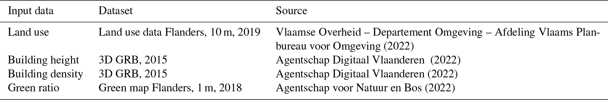
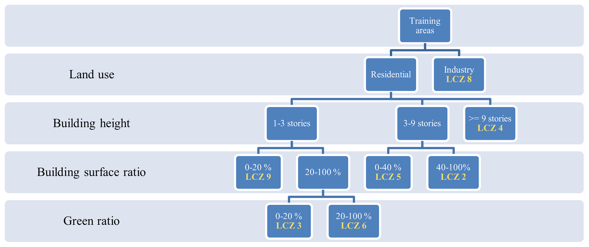

Figure B2Training areas used for the creation of the LCZ map. Delineation is based on land use, building height, building density and green ratio data. The background map is from Esri (ESRI World Topographic Map, 2022).
Table B2Confusion matrix LCZ map. The matrix summarises the number of cells wrongly or correctly classified for each LCZ class. The user accuracy (UA) and producer accuracy (PA) for each LCZ class and the overall accuracy are also included. For each LCZ, the number of cells correctly classified are shown in bold.

A qualitative assessment of the data quality was performed by making scatterplots of these variables for the LC-R stations compared to the AWSs (Fig. C1).
Overall, the measured parameters are within the accuracy given by the manufacturer. There are, however, deviations in the wind and radiation measurement that are attributable to the small location differences (of the order of metres) between the LC-R stations and the official sensors. For wind, we compared the LC-R data with professional 2 m wind measurements, but this height is in fact not the standard measurement height for wind because too many ground effects are still in play at this height. With respect to radiation, we previously mentioned the design flaw regarding the wind vane casting a shadow, but high nearby trees can also influence the measurements for low solar elevations (in the case of LC-R01 and LC-R02).

Figure C1Scatterplots of LC-R versus AWS dew point temperature, humidity, radiation and wind speed for each reference station: LC-R01, LC-R02, LC-R04 and LC-R05. The identity line is shown in black. The colour scale indicates the density of observations, with yellow indicating the highest and purple indicating the lowest. The scatterplots include all measurements between the installation date of each LC-R and December 2021. For each variable, the same ranges are used on the x and y axes.
In Sect. 5, the RF model is applied to the LC-R dataset to obtain a corrected temperature for each observation. These results could be biased because the RF model is trained on 60 % of the LC-R dataset and then applied to the complete LC-R dataset. To account for this, we applied the prediction model to both the complete dataset and the test dataset (which was not used for training the model). The outcome for each LC-R is listed in Table D1. It can be noted that mean T difference remains equal for both datasets, and the standard deviation does slightly increase by 0.5 to 0.7 ∘C when using the test dataset only. The mean temperature difference ± standard deviation for all LC-R stations increases from 0.00 ± 0.22 to 0.00 ± 0.28 ∘C.
For comparison, the histograms and heat maps of the temperature difference () using the complete and test dataset only have been added in Figs. D1, D2 and D3. Only slight differences (smaller than 0.1 ∘C) exist between the ΔT for the complete dataset and ΔT for the test dataset. The diurnal and seasonal pattern is still corrected for (Fig. D2). Moreover, the effects of wind speed and radiation are effectively eliminated (Fig. D3).
Table D1Comparison of the obtained T difference () when using the test LC-R dataset and the complete LC-R dataset.
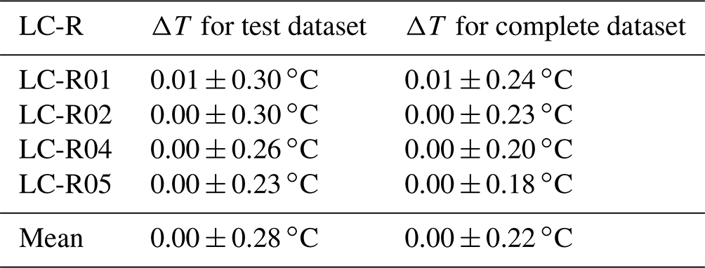
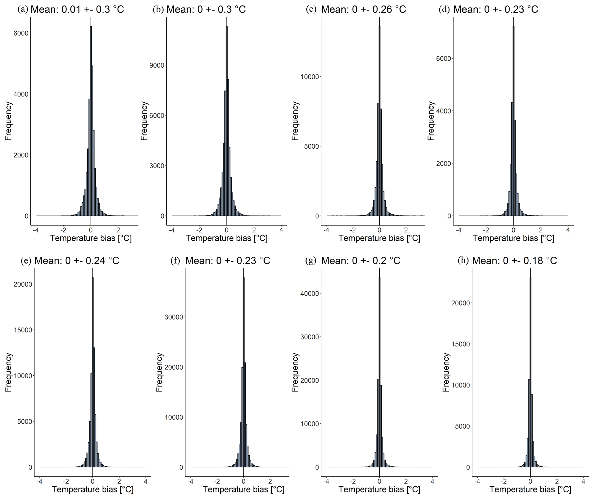
Figure D1Same as Fig. 9 but for QC level 3. Comparison between ΔT for the test dataset (a–d) and ΔT for the complete dataset (e–h).
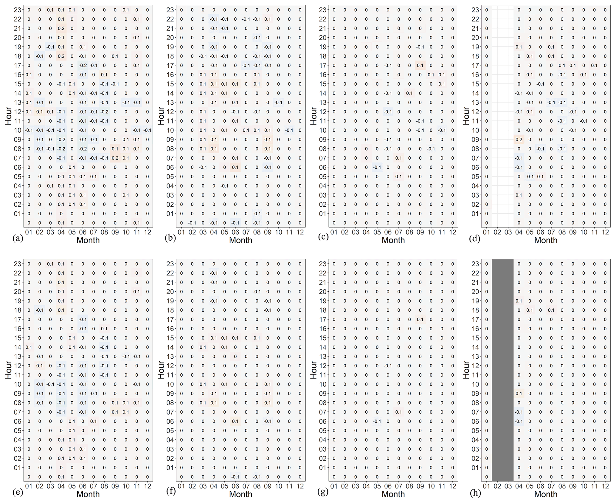
Figure D2Same as Fig. 10 but for QC level 3. Comparison between ΔT for the test dataset (a–d) and ΔT for the complete dataset (e–h).
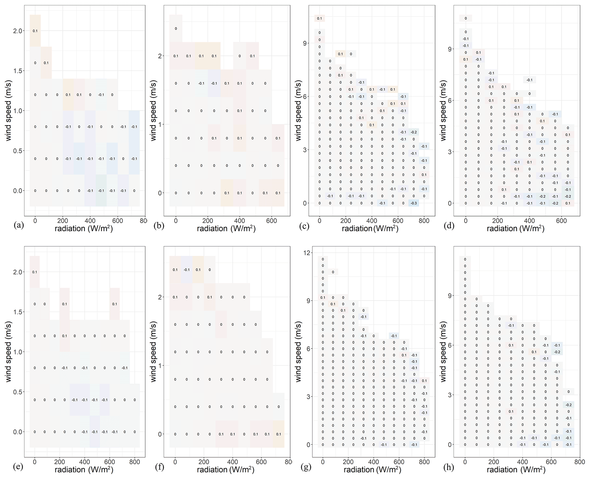
Figure D3Same as Fig. 11 but for QC level 3. Comparison between ΔT for the test dataset (a–d) and ΔT for the complete dataset (e–h).
All authors contributed to the design of the weather station network. EB and MR practically implemented the design and collected the CWS data, MR assembled AWS data, and EB processed all of the data used. All authors contributed to the design of the QC method; EB did the programming for the QC. EB carried out all analyses and primarily wrote the manuscript. All authors discussed the results and contributed to writing the manuscript.
The contact author has declared that none of the authors has any competing interests.
Publisher's note: Copernicus Publications remains neutral with regard to jurisdictional claims in published maps and institutional affiliations.
The authors thank the many people who have contributed to the establishment and maintenance of the Leuven.cool project. In particular, we are grateful to all citizens and private companies of/within Leuven who voluntary made their garden/terrain available for our research. We also wish to thank Tim Guily (city of Leuven) and Hanne Wouters (Leuven 2030) for their logistic support as well as Margot Verhulst, Jordan Rodriguez Milis, Remi Chevalier, Jingli Yan, Floris Abrams, Jonas Verellen and Lennert Destadsbader (KU Leuven) for their technical support during the realisation of the network. We further thank Clémence Dereux, who developed a basis for the random forest correction model as a RMI job student in 2019. Lastly, we are grateful to Rafail Varonos (Leuven 2030) for ICT support. The protocol of this study was approved by the Social and Societal Ethics Committee of KU Leuven (G-2019 06 1674). The weather stations used in this study were sponsored by both the city of Leuven and KU Leuven. Eva Beele holds an SB doctoral fellowship from the Research Foundation – Flanders (FWO; grant no. 1SE0621N).
This research has been supported by the Research Foundation – Flanders (FWO; grant no. 1SE0621N).
This paper was edited by David Carlson and reviewed by Daniel Fenner and one anonymous referee.
Agentschap Digitaal Vlaanderen: 3D GRB, Geopunt [data set], https://www.geopunt.be/catalogus/datasetfolder/42ac31a7-afe6-44c4-a534-243814fe5b58, last access: 1 March 2022.
Agentschap voor Natuur en Bos: Groenkaart Vlaanderen 2018, Geopunt [data set], https://www.geopunt.be/catalogus/datasetfolder/2c64ca0c-5053-4a66-afac-24d69b1a09e7, last access: 1 March 2022.
Aigang, L., Tianming, W., Shichang, K., and Deqian, P.: On the Relationship between Latitude and Altitude Temperature Effects, in: 2009 International Conference on Environmental Science and Information Application Technology, 55–58, https://doi.org/10.1109/ESIAT.2009.335, 2009.
Ahrens, C. D.: Meteorology Today: An Introduction to Weather, Climate, and the Environment, 9th Edn., Brooks/Cole, 549 pp., 2009.
Arnfield, A. J.: Two decades of urban climate research: A review of turbulence, exchanges of energy and water, and the urban heat island, Int. J. Climatol., 23, 1–26, https://doi.org/10.1002/joc.859, 2003.
Båserud, L., Lussana, C., Nipen, T. N., Seierstad, I. A., Oram, L., and Aspelien, T.: TITAN automatic spatial quality control of meteorological in-situ observations, Adv. Sci. Res., 17, 153–163, https://doi.org/10.5194/asr-17-153-2020, 2020.
Bassani, F., Garbero, V., Poggi, D., Ridolfi, L., Von Hardenberg, J., and Milelli, M.: Urban Climate An innovative approach to select urban-rural sites for Urban Heat Island analysis: the case of Turin (Italy), Urban Clim., 42, 101099, https://doi.org/10.1016/j.uclim.2022.101099, 2022.
Beele, E., Reyniers, M., Aerts, R., and Somers, B.: Replication Data for: Quality control and correction method for air temperature data from a citizen science weather station network in Leuven, Belgium, KU Leuven RDR [data set], https://doi.org/10.48804/SSRN3F, 2022.
Bell, S., Cornford, D., and Bastin, L.: How good are citizen weather stations? Addressing a biased opinion, Weather, 70, 75–84, https://doi.org/10.1002/wea.2316, 2015.
Brans, K. I., Tüzün, N., Sentis, A., De Meester, L., and Stoks, R.: Cryptic eco-evolutionary feedback in the city: Urban evolution of prey dampens the effect of urban evolution of the predator, J. Anim. Ecol., 91, 514–526, https://doi.org/10.1111/1365-2656.13601, 2022.
Castell, N., Dauge, F. R., Schneider, P., Vogt, M., Lerner, U., Fishbain, B., Broday, D., and Bartonova, A.: Can commercial low-cost sensor platforms contribute to air quality monitoring and exposure estimates?, Environ. Int., 99, 293–302, https://doi.org/10.1016/j.envint.2016.12.007, 2017.
Chapman, L., Bell, C., and Bell, S.: Can the crowdsourcing data paradigm take atmospheric science to a new level? A case study of the urban heat island of London quantified using Netatmo weather stations, Int. J. Climatol., 37, 3597–3605, https://doi.org/10.1002/joc.4940, 2017.
Chen, J., Saunders, K., and Whan, K.: Quality control and bias adjustment of crowdsourced wind speed observations, Q. J. Roy. Meteor. Soc., 147, 3647–3664, https://doi.org/10.1002/qj.4146, 2021.
Cornes, R. C., Dirksen, M., and Sluiter, R.: Correcting citizen-science air temperature measurements across the Netherlands for short wave radiation bias, Meteorol. Appl., 27, 1–16, https://doi.org/10.1002/met.1814, 2020.
Demografie: https://leuven.incijfers.be/dashboard/dashboard/demografie, last access: 15 December 2021.
Demoury, C., Aerts, R., Vandeninden, B., Van Schaeybroeck, B., and De Clercq, E. M.: Impact of Short-Term Exposure to Extreme Temperatures on Mortality: A Multi-City Study in Belgium, Int. J. Env. Res. Pub. He., 19, 3763, https://doi.org/10.3390/ijerph19073763, 2022.
Demuzere, M., Hankey, S., Mills, G., Zhang, W., Lu, T., and Bechtel, B.: Combining expert and crowd-sourced training data to map urban form and functions for the continental US, Sci. Data, 7, 1–13, https://doi.org/10.1038/s41597-020-00605-z, 2020.
De Ridder, K., Lauwaet, D., and Maiheu, B.: UrbClim – A fast urban boundary layer climate model, Urban Clim., 12, 21–48, https://doi.org/10.1016/j.uclim.2015.01.001, 2015.
De Troeyer, K., Bauwelinck, M., Aerts, R., Profer, D., Berckmans, J., Delcloo, A., Hamdi, R., Van Schaeybroeck, B., Hooyberghs, H., Lauwaet, D., Demoury, C., and Van Nieuwenhuyse, A.: Heat related mortality in the two largest Belgian urban areas: A time series analysis, Environ. Res., 188, 109848, https://doi.org/10.1016/j.envres.2020.109848, 2020.
de Vos, L., Leijnse, H., Overeem, A., and Uijlenhoet, R.: The potential of urban rainfall monitoring with crowdsourced automatic weather stations in Amsterdam, Hydrol. Earth Syst. Sci., 21, 765–777, https://doi.org/10.5194/hess-21-765-2017, 2017.
de Vos, L., Leijnse, H., Overeem, A., and Uijlenhoet, R.: Quality Control for Crowdsourced Personal Weather Stations to Enable Operational Rainfall Monitoring, Geophys. Res. Lett., 46, 8820–8829, https://doi.org/10.1029/2019GL083731, 2019.
de Vos, L., Droste, A. M., Zander, M. J., Overeem, A., Leijnse, H., Heusinkveld, B. G., Steeneveld, G. J., and Uijlenhoet, R.: Hydrometeorological monitoring using opportunistic sensing networks in the Amsterdam metropolitan area, B. Am. Meteorol. Soc., 101, E167–E185, https://doi.org/10.1175/BAMS-D-19-0091.1, 2020.
EEA: Assessing air quality through citizen science, Copenkagen, 63 pp., https://doi.org/10.2800/619, 2019.
ESRI World Topographic Map: http://www.arcgis.com/home/item.html?id=30e5fe3149c34df1ba922e6f5bbf808f, last access: 1 March 2022.
Feichtinger, M., Wit, R. De, Goldenits, G., Kolejka, T., and Hollósi, B.: Urban Climate Case-study of neighborhood-scale summertime urban air temperature for the City of Vienna using crowd-sourced data, Urban Clim., 32, 1–12, https://doi.org/10.1016/j.uclim.2020.100597, 2020.
Fenner, D., Meier, F., Bechtel, B., Otto, M., and Scherer, D.: Intra and inter “local climate zone” variability of air temperature as observed by crowdsourced citizen weather stations in Berlin, Germany, Meteorol. Z., 26, 525–547, https://doi.org/10.1127/metz/2017/0861, 2017.
Fenner, D., Bechtel, B., Demuzere, M., Kittner, J., and Meier, F.: CrowdQC + – A Quality-Control for Crowdsourced Air-Temperature Observations Enabling World-Wide Urban Climate Applications, Front. Environ. Sci., 9, 1–21, https://doi.org/10.3389/fenvs.2021.720747, 2021.
Hammerberg, K., Brousse, O., Martilli, A., and Mahdavi, A.: Implications of employing detailed urban canopy parameters for mesoscale climate modelling: a comparison between WUDAPT and GIS databases over Vienna, Austria, Int. J. Climatol., 38, e1241–e1257, https://doi.org/10.1002/joc.5447, 2018.
Heaviside, C., Macintyre, H., and Vardoulakis, S.: The Urban Heat Island: Implications for Health in a Changing Environment, Curr. Environ. Heal. Rep., 4, 296–305, https://doi.org/10.1007/s40572-017-0150-3, 2017.
IPCC: Climate Change 2021: The Physical Science Basis. Contribution of Working Group I to the Sixth Assessment Report of the Intergovernmental Panel on Climate Change, edited by: Masson-Delmotte, V., Zhai, P., Pirani, A., Connors, S. L., Péan, C., Berger, S., Caud, N., Chen, Y., Goldfarb, L., Gomis, M. I., Huang, M., Leitzell, K., Lonnoy, E., Matthews, J. B. R., Maycock, T. K., Waterfield, T., Yelekçi, O., Yu, R., and Zhou, B., Cambridge University Press, Cambridge, United Kingdom and New York, NY, USA, in press, https://doi.org/10.1017/9781009157896, 2021.
Jenkins, G.: A comparison between two types of widely used weather stations, Weather, 69, 105–110, https://doi.org/10.1002/wea.2158, 2014.
Kidder, S. Q. and Essenwanger, O. M.: The Effect of Clouds and Wind on the Difference in Nocturnal Cooling Rates between Urban and Rural Areas, J. Appl. Meteorol., 34, 2440–2448, https://doi.org/10.1175/1520-0450(1995)034<2440:TEOCAW>2.0.CO;2, 1995.
Kirk, P. J., Clark, M. R., and Creed, E.: Weather Observations Website, Weather, 76, 47–49, https://doi.org/10.1002/wea.3856, 2020.
Kottek, M., Grieser, J., Beck, C., Rudolf, B., and Rubel, F.: World map of the Köppen-Geiger climate classification updated, Meteorol. Z., 15, 259–263, https://doi.org/10.1127/0941-2948/2006/0130, 2006.
Kousis, I., Pigliautile, I., and Pisello, A. L.: Intra-urban microclimate investigation in urban heat island through a novel mobile monitoring system, Sci. Rep., 11, 1–17, https://doi.org/10.1038/s41598-021-88344-y, 2021.
Lefebvre, W., Vercauteren, J., Schrooten, L., Janssen, S., Degraeuwe, B., Maenhaut, W., de Vlieger, I., Vankerkom, J., Cosemans, G., Mensink, C., Veldeman, N., Deutsch, F., Van Looy, S., Peelaerts, W., and Lefebre, F.: Validation of the MIMOSA-AURORA-IFDM model chain for policy support: Modeling concentrations of elemental carbon in Flanders, Atmos. Environ., 45, 6705–6713, https://doi.org/10.1016/j.atmosenv.2011.08.033, 2011.
Leuven.cool: https://www.leuven.cool/, last access: 15 December 2020.
Longman, R. J., Giambelluca, T. W., Nullet, M. A., Frazier, A. G., Kodama, K., Crausbay, S. D., Krushelnycky, P. D., Cordell, S., Clark, M. P., Newman, A. J., and Arnold, J. R.: Compilation of climate data from heterogeneous networks across the Hawaiian Islands, Sci. Data, 5, 180012, https://doi.org/10.1038/sdata.2018.12, 2018.
Mandement, M. and Caumont, O.: Contribution of personal weather stations to the observation of deep-convection features near the ground, Nat. Hazards Earth Syst. Sci., 20, 299–322, https://doi.org/10.5194/nhess-20-299-2020, 2020.
Masson, V., Le Moigne, P., Martin, E., Faroux, S., Alias, A., Alkama, R., Belamari, S., Barbu, A., Boone, A., Bouyssel, F., Brousseau, P., Brun, E., Calvet, J.-C., Carrer, D., Decharme, B., Delire, C., Donier, S., Essaouini, K., Gibelin, A.-L., Giordani, H., Habets, F., Jidane, M., Kerdraon, G., Kourzeneva, E., Lafaysse, M., Lafont, S., Lebeaupin Brossier, C., Lemonsu, A., Mahfouf, J.-F., Marguinaud, P., Mokhtari, M., Morin, S., Pigeon, G., Salgado, R., Seity, Y., Taillefer, F., Tanguy, G., Tulet, P., Vincendon, B., Vionnet, V., and Voldoire, A.: The SURFEXv7.2 land and ocean surface platform for coupled or offline simulation of earth surface variables and fluxes, Geosci. Model Dev., 6, 929–960, https://doi.org/10.5194/gmd-6-929-2013, 2013.
Meier, F., Fenner, D., Grassmann, T., Otto, M., and Scherer, D.: Crowdsourcing air temperature from citizen weather stations for urban climate research, Urban Clim., 19, 170–191, https://doi.org/10.1016/j.uclim.2017.01.006, 2017.
Muller, C. L., Chapman, L., Johnston, S., Kidd, C., Illingworth, S., Foody, G., Overeem, A., and Leigh, R. R.: Crowdsourcing for climate and atmospheric sciences: Current status and future potential, Int. J. Climatol., 35, 3185–3203, https://doi.org/10.1002/joc.4210, 2015.
Napoly, A., Grassmann, T., Meier, F., and Fenner, D.: Development and Application of a Statistically-Based Quality Control for Crowdsourced Air Temperature Data, Front. Earth Sci., 6, 1–16, https://doi.org/10.3389/feart.2018.00118, 2018.
Nipen, T. N., Seierstad, I. A., Lussana, C., Kristiansen, J., and Hov, Ø.: Adopting citizen observations in operational weather prediction, B. Am. Meteorol. Soc., 101, E43–E57, https://doi.org/10.1175/BAMS-D-18-0237.1, 2020.
Oke, T. R.: City size and the urban heat island, Atmos. Environ., 7, 769–779, 1973.
Qian, Y., Zhou, W., Hu, X., and Fu, F.: The Heterogeneity of Air Temperature in Urban Residential Neighborhoods and Its Relationship with the Surrounding Greenspace, Remote Sens., 10, 965, https://doi.org/10.3390/rs10060965, 2018.
Rizwan, A. M., Dennis, L. Y. C., and Lia, C.: A review on the generation, determination and mitigation of Urban Heat Island, J. Environ. Sci., 20, 120–128, https://doi.org/10.1016/S1001-0742(08)60019-4, 2008.
RMI: Klimaatstatistieken van de Belgische gemeenten: Leuven, Royal Meteorological Institute of Belgium, Leuven, 5 pp., https://www.meteo.be/resources/climatology/climateCity/pdf/climate_INS24062_9120_nl.pdf (last access: 14 October 2022), 2020.
Sgoff, C., Acevedo, W., Paschalidi, Z., Ulbrich, S., Bauernschubert, E., Kratzsch, T., and Potthast, R.: Assimilation of crowd-sourced surface observations over Germany in a regional weather prediction system, Q. J. Roy. Meteor. Soc., 148, 1752–1767, https://doi.org/10.1002/qj.4276, 2022.
Sotelino, L. G., De Coster, N., Beirinckx, P., and Peeters, P.: Intercomparison of Shelters in the RMI AWS Network, WMO-CIMO, P1_26, Geneva, Switzerland, https://www.wmocimo.net/wp-content/uploads/P1_26_Sotelino_teco_2018_lgs.pdf (last access: 14 October 2022), 2018.
Stewart, I. D.: A systematic review and scientific critique of methodology in modern urban heat island literature, Int. J. Climatol., 31, 200–217, https://doi.org/10.1002/joc.2141, 2011.
Stewart, I. D. and Oke, T. R.: Local climate zones for urban temperature studies, B. Am. Meteorol. Soc., 93, 1879–1900, https://doi.org/10.1175/BAMS-D-11-00019.1, 2012.
UN, Population Division: World Urbanization Prospects: The 2018 Revision (ST/ESA/SER.A/420), New York, United Nations, 126 pp., https://population.un.org/wup/publications/Files/WUP2018-Report.pdf (last access: 14 October 2022), 2019
Venter, Z. S., Chakraborty, T., and Lee, X.: Crowdsourced air temperatures contrast satellite measures of the urban heat island and its mechanisms, Sci. Adv., 7, 1–9, https://doi.org/10.1126/sciadv.abb9569, 2021.
Verdonck, M. L., Demuzere, M., Hooyberghs, H., Beck, C., Cyrys, J., Schneider, A., Dewulf, R., and Van Coillie, F.: The potential of local climate zones maps as a heat stress assessment tool, supported by simulated air temperature data, Landscape Urban Plan., 178, 183–197, https://doi.org/10.1016/j.landurbplan.2018.06.004, 2018.
Vlaamse Overheid – Departement Omgeving – Afdeling Vlaams Planbureau voor Omgeving: Landgebruik – Vlaanderen – toestand 2019: https://www.geopunt.be/catalogus/datasetfolder/fe979929-a2b5-4353-94c5-608c4b109dc6, last access: 1 March 2022.
Weather Observations Website – Belgium: https://wow.meteo.be/nl/, last access: 1 March 2022.
WMO: Guide to meteorological instruments and methods of observation, Volume I – Measurement of Meteorological Variables, Geneva, 573 pp., https://library.wmo.int/doc_num.php?explnum_id=10616 (last access: 14 October 2022), 2018.
Yang, Q., Huang, X., Yang, J., and Liu, Y.: The relationship between land surface temperature and artificial impervious surface fraction in 682 global cities: Spatiotemporal variations and drivers, Environ. Res. Lett., 16, 024032, https://doi.org/10.1088/1748-9326/abdaed, 2021.
- Abstract
- Introduction
- Materials and methods
- Description of the quality control and correction method
- Evaluation of the quality control and correction method
- Application of the QC method to the stations in the study area
- Application potential of the quality-controlled and corrected Leuven.cool dataset
- Code and data availability
- Conclusions
- Appendix A: Specifications of the WH2600 digital weather station
- Appendix B: Specifications of the LCZ map
- Appendix C: Quality control of other Leuven.cool variables
- Appendix D: Application of the RF model on the LC-R dataset
- Author contributions
- Competing interests
- Disclaimer
- Acknowledgements
- Financial support
- Review statement
- References