GLOBMAP SWF: a global annual surface water cover frequency dataset during 2000–2020

The extent of surface water has been changing significantly due to climatic change and human activities. However, it is challenging to capture the interannual changes of inland water bodies due to their high seasonal variation and abrupt change. In this paper, a global annual surface water cover frequency dataset (GLOBMAP SWF) was generated from the MODIS land surface reflectance products during 2000–2020 to describe the seasonal and interannual dynamics of surface water. Surface water cover frequency (SWF) was proposed as the percentage of the time period when a pixel is covered by water in a year. Instead of determination of the water directly, the SWF was estimated indirectly by identifying land observations among annual clear-sky observations to reduce the influence of clouds and variability of water bodies and surface background characteristics, which helps to improve the applicability of the algorithm for different regions across the globe. The generated dataset shows better performances for frozen water, saline lakes, bright surfaces and regions with frequent cloud cover compared with the two high-frequency surface water datasets derived from MODIS data, and it captures more intermittent surface water but may underestimate small water bodies when compared with two high-resolution datasets derived from Landsat data. Compared with the high-resolution SWF maps extracted from Sentinel-1 data in eight regions that cover lakes, rivers and wetlands, the R² reaches 0.46 to 0.97, RMSE ranges from 7.24 % to 22.62 %, and MAE is between 2.07 % and 7.15 %. In 2020, the area of global maximum surface water extent is 3.38×10⁶ km², of which the permanent surface water accounts for approximately 54 % (1.83×10⁶ km²), and the other 46 % is intermittent surface water (1.55×10⁶ km²). The area of global maximum and permanent surface water has been shrinking since 2001, with a change rate of −7577 and −4315 km² yr⁻¹ (p<0.05), respectively, while the intermittent surface water with the SWF above 50 % has been expanding (1368 km² yr⁻¹, p<0.01). This dataset can be used to analyze the interannual variation and change trend of highly dynamic inland waters extent with consideration of its seasonal variation. The GLOBMAP SWF data are available at https://doi.org/10.5281/zenodo.6462883 (Liu and Liu, 2022).

1 Introduction

Surface water, comprised of natural lakes, rivers, reservoirs and seasonally flooded waters, supplies water resources for maintenance of the functions of terrestrial ecosystem and livelihoods of human society. It plays a vital role in the global hydrological cycle, carbon cycle and climate system (Karlsson et al., 2021) and also provides habitats for aquatic animals and plants. Inland waters usually show significant interannual and seasonal variations due to seasonality and changes of precipitation and evaporation as well as human activities (Konapala et al., 2020). The extent of surface water is suggested to be a sensitive indicator of climatic change and also responds to human activities (Zhang et al., 2019). And the changes of surface water extent impact global hydrological and carbon cycles and the availability of water resources, which would affect human society and ecosystems' sustainability (Padron et al., 2020; Miara et al., 2017; Ran et al., 2021).

Surface water has been monitored using repeated satellite observations of the Earth's surface. The extent of inland water bodies has been mapped with active and passive microwave observations, which can penetrate clouds and vegetation to a certain extent. Several global surface water datasets have been generated from microwave observations and provide monthly or weekly water cover maps at a spatial resolution of dozens of kilometers. For example, the Global Inundation Extent from Multi-Satellites (GIEMS) datasets were created by fusing multiple satellite observations of passive and active microwaves along with visible and near-infrared imagery, which describe the monthly distribution of global surface water extent at 0.25^∘ resolution (Prigent et al., 2007; Papa et al., 2010; Prigent et al., 2020). A weekly inland water fraction dataset (Global-SWAF) was produced at a spatial resolution of 25 km based on L-band multi-angle and dual-polarization microwave satellite data from the Soil Moisture Ocean Salinity (SMOS) mission over the period of 2010 to 2019 (Al Bitar et al., 2020). In recent years, with the availability of the Sentinel-1 C-band Synthetic Aperture Radar (SAR) data, a few regional 10 m resolution water body datasets have been developed, such as the High Spatial-Temporal Water Body dataset in China (HSWDC) during 2016–2018 (Li et al., 2020). But these high-resolution datasets can only cover the period since the launch of Sentinel-1.

Surface water was also mapped with optical satellite data, which can provide long-term observations of the Earth's surface at tens to hundreds of meters' resolution. Several global 30 m resolution surface water datasets have been generated from optical high-resolution satellite data, such as Landsat (e.g., Liao et al., 2014; Pekel et al., 2016; Feng et al., 2016; Pickens et al., 2020). These datasets can describe the detailed spatial distribution of inland water bodies, usually the maximum surface water extent during the observing period. Surface water generally shows remarkable seasonal and interannual variations and may fluctuate abruptly during a short period due to rainfall or reservoir constructions (Berghuijs et al., 2014; Lutz et al., 2014; Pickens et al., 2020). The approaches based on high-spatial-resolution optical images only provide a limited number of the snapshots of water cover and their average change rate of area over a specific period of several years. The sparse temporal sampling of these satellites makes it difficult for them to capture interannual and seasonal variations of inland waters, even misrepresented by the abrupt fluctuation of water cover.

The Moderate Resolution Imaging Spectroradiometer (MODIS) carried on the Terra and Aqua satellites, with its daily revisiting period, provides a powerful tool to capture the dynamics of surface water. Several global and regional high-frequency surface water products have been generated using MODIS data. Daily global datasets of inland water bodies were generated at 250–500 m resolution (Klein et al., 2017; Ji et al., 2018), and 8 d datasets were also created at 250 m resolution at global (Han and Niu, 2020) and regional (Lu et al., 2019b) scales. Several datasets for reservoirs and large lakes were also produced from MODIS observations at 8 d temporal and 250–500 m spatial resolution (Khandelwal et al., 2017; Tortini et al., 2020; Li et al., 2021). These high-frequency datasets generally directly identify water pixels for each daily or multi-day composite satellite scene using the following steps. The satellite observation is usually preprocessed to exclude the effects of cloud, ice/snow and shadow. Then, the water pixels are identified for clear-sky observations using threshold or classification methods based on reflectance on the visible, near-infrared (NIR), and shortwave infrared (SWIR) bands and spectral indices. Finally, the missing data from clouds and other contaminations are usually filled using temporal interpolation to generate a gap-free time series of inland waters. The high-frequency datasets can capture the seasonal variation and short-term fluctuation of surface water extent with their daily or 8 d time-series maps. However, since the timing of precipitation and human activity (such as reservoir impoundment and drainage) may shift among years, it would be incomparable for the snapshot of surface water even acquired on the same day of the year (DOY), which would conceal the real change trend when directly using these high-frequency datasets. Additionally, clouds and variable characteristics of the water body and surface background may affect the performance of the water mapping algorithm, making it challenging to accurately extract surface water cover at a global scale. For example, special water bodies, such as frozen water and saline lakes, may show different spectral characteristics compared with those of pure water and reduce the applicability of the algorithm, and it is difficult to accurately identify all clouds and snow/ice pixels, which would introduce uncertainties to the estimation results.

In this paper, a global annual surface water cover frequency dataset (GLOBMAP SWF) was generated from MODIS land surface reflectance data with a resolution of 500 m from 2000 to 2020. The seasonal variation of surface water was simplified to the percentage of the time period when a pixel is covered by water in a year (surface water cover frequency, SWF) to characterize the seasonal and interannual dynamics of surface water. The SWF transforms a discrete variable (water or land) into a continuous variable that can describe the distribution and life cycle of intermittent surface water. It can help to avoid the interannual mismatch issue mentioned above by excluding the influence of different occurrence periods of water cover. The SWF was estimated from MODIS observations annually. The estimation results were compared with two high-frequency surface water products derived from MODIS and two high-spatial-resolution products derived from Landsat and validated with the SWF maps derived from Sentinel-1 SAR data. Several examples were also provided to demonstrate its application for the characterization of seasonal and interannual dynamics of inland water bodies.

2 Datasets

2.1 MODIS land surface reflectance products for surface water extraction

The MOD09A1 land surface reflectance product (Version 6) (https://search.earthdata.nasa.gov/, last access: 20 November 2021) was used to generate the SWF dataset. This product contains the atmospherically corrected surface spectral reflectance of MODIS 1–7 bands, including three visible bands (red, blue and green), one NIR band and three SWIR bands (1.2, 1.6 and 2.1 µm) (Vermote, 2015). The 8 d composited surface reflectance with low view angle and absence of clouds or cloud shadows and aerosol loading if available are provided at 500 m resolution in the sinusoidal projection. The red, NIR and SWIR bands are sensitive to the boundaries and properties of water, land, cloud and aerosols. Here, the reflectance of MODIS Band 1 (red, 0.620–0.670 µm), Band 2 (NIR, 0.841–0.876 µm) and Band 7 (SWIR, 2.105–2.155 µm) bands was utilized to estimate the SWF. Among them, the red and SWIR bands were used to determine land observations, and the NIR band was used to extract the annual maximum surface water extent and distinguish water from cloud and ice/snow.

2.2 Digital elevation model for mountain shadow exclusion

The digital elevation model (DEM) of the U.S. Geological Survey (USGS) Global 30-Arc-Second Elevation (GTOPO30) (https://earthexplorer.usgs.gov/, last access: 20 October 2021) was used to exclude mountain shadow in the extraction of the annual maximum surface water extent. This product provides a DEM of the entire Earth's surface with geographic coordinates and horizontal datum of WGS84 in a resolution of 30 arcsec (approximately 900 m). The elevation data were derived from eight sources of topographic information, including Digital Terrain Elevation Data, Digital Chart of the World, USGS 1^∘ DEMs, Army Map Service 1:1 000 000-scale maps, International Map of the World 1:1 000 000-scale maps, Peru 1:1 000 000-scale map, New Zealand DEM and Antarctic Digital Database. The elevation data were transferred to the sinusoidal projection to be consistent with that of MODIS land surface reflectance data and used to calculate the terrain slope for mountain shadow exclusion.

2.3 Surface water datasets for comparison

Two high-frequency surface water datasets derived from MODIS data and two high-resolution datasets derived from Landsat data were employed for comparison purposes, including the global surface water change database from Ji et al. (2018) (hereafter referred to as GSWCD) and Inland Surface Water Dataset in China (ISWDC) (Lu et al., 2019b), Global Surface Water dataset (GSW) from Pekel et al. (2016) and the global inland water dataset derived by the Global Land Analysis and Discovery laboratory (hereafter referred to as GLAD) (Pickens et al., 2020).

The GSWCD provides global daily water maps at 500 m resolution during 2001–2016 derived from the MODIS daily reflectance time series (http://data.ess.tsinghua.edu.cn/modis_500_2001_2016_waterbody.html, last access: 12 January 2022). Water was identified on each single-date reflectance image with the assumption that reflectance of water at the visible bands should be higher than at the SWIR bands, as well as thresholds of reflectance in visible and SWIR bands. For those pixels with low reflectance in visible bands, the spectral property assumption may not be exhibited, thresholds of visible and SWIR bands reflectance were used to identify water pixels and normalized difference vegetation index (NDVI) was used to reduce the confusion between water and dense vegetation. The shadow effects caused by mountains and clouds were reduced with a terrain slope derived from ASTER DEM data and cloud shadow flag of MODIS state quality assurance (QA) layer, respectively. The cloud, ice/snow and no valid data were labeled with MODIS state QA layer and land surface temperature data, and cloud and no valid data were filled with temporal–spatial interpolation to produce a gap-free time series. The producer's accuracy and user's accuracy of the GSWCD product were reported better than 90 % when compared with classification results derived from Landsat images and manually interpreted samples.

The ISWDC product maps water bodies larger than 0.0625 km² within the land mass of China for the period 2000–2016 with 8 d temporal and 250 m spatial resolution (https://doi.org/10.5281/zenodo.2616035; Lu et al., 2019a). The surface water boundary was extracted based on the modified Otsu threshold method with reflectance of MODIS NIR band. The threshold value was determined for four seasons with 423 selected samples of lakes and rivers. The interferences were removed with a terrain slope derived from SRTM DEM data. The producer's accuracy and user's accuracy of the ISWDC product were reported to be 88.95 % and 91.13 % when compared with samples from lakes and rivers derived from the China national 30 m land cover dataset (Liu et al., 2014).

The GSW product provides global surface water maps for the period 1984–2020 with 30 m resolution (https://global-surface-water.appspot.com/download, last access: 10 August 2022). The pixels in Landsat 5, 7 and 8 data were classified as open water, land or non-valid observation using the combination of expert systems, visual analytics and evidential reasoning. The classifier produces less than 1 % of false water detections and misses less than 5 % of water when measured using over 40 000 reference points. A seasonality dataset is contained in the GSW products to describe the intra-annual distribution of water and used to compare with our estimation results. A permanent water surface is underwater throughout 12 months of the year (with a seasonality value of 12), while a seasonal water surface has a value less than 12. For lakes that freeze for part of the year, the dataset treats ice as a non-valid observation, and the observation period corresponds only to the unfrozen months.

The GLAD product maps global inland water for the period 1999–2020 with 30 m resolution (https://www.glad.umd.edu/dataset/global-surface-water-dynamics, last access: 10 August 2022). The land and water were classified in all Landsat 5, 7 and 8 scenes and performed a time-series analysis to produce maps that characterize interannual and intra-annual open surface water dynamics. Each Landsat scene was classified into land, water, cloud, shadow, haze and snow/ice with ensembles of classification trees. The producer's accuracy and user's accuracy of the GLAD monthly mapped water class were reported to be 96.0 % and 93.7 % when compared with reference sample data. The annual water percent dataset is contained in the GLAD products to characterize the seasonality of the water cover and used to compare with our results. The land and water observations of a given pixel were summed per month and aggregated into water presence frequency, measured by the percent of clear observations flagged as water.

2.4 Datasets for validation

The estimation results were validated with the SWF maps extracted from Sentinel-1 data. To evaluate the performance of our dataset for different surface water types, permanent and seasonal waters, and different latitudes, as well as the presence of frequent cloud cover, eight regions were selected for validation, including Lake Albert in the Democratic Republic of the Congo and Uganda (30.98^∘ E, 1.74^∘ N), Lake Mai-Ndombe in the Democratic Republic of the Congo in the southwestern part of Congo Basin (18.32^∘ E, 2.07^∘ S), the Amazon River and Taparus River in western Amazon in Brazil (54.87^∘ W, 2.16^∘ S), wetlands in western Bangladesh (91.12^∘ E, 24.65^∘ N), Lake Winnipegosis in Canada (99.91^∘ W, 52.61^∘ N), lakes in western Russia (31.00^∘ E, 64.10^∘ N), Lake Maggiore in Italy (8.65^∘ E, 45.90^∘ N) and Lake Wakatipu in New Zealand (168.55^∘ E, 45.10^∘ S). These areas cover major types of inland water bodies, including lakes, rivers and wetlands. Among them, the six lake regions and the Taparus River are dominated by permanent surface water, the Amazon River has seasonal water cover and wetlands in western Bangladesh are dominated by seasonal surface water. Lake Albert, Lake Mai-Ndombe, the Amazon River, the Taparus River and wetlands in western Bangladesh are in the tropics and subtropics. Cloud and rain should frequently occur in these four regions, especially for the Amazon River, Taparus River, and Lake Mai-Ndombe in the Amazon and Congo Basin respectively, which helps to evaluate the performance in frequently cloud-covered areas. Lake Maggiore and Lake Wakatipu are in the middle latitudes of the Northern and Southern Hemisphere, respectively. The former is surrounded by mountains in the Alps in northern Italy, which shows an example of the performance in mountainous regions. Lake Winnipegosis and lakes in western Russia are in high latitudes of the Northern Hemisphere, where a large number of small water bodies are concentrated.

The Sentinel-1 mission images the entire Earth every 6 d with a constellation of two satellites orbiting 180^∘ apart, and the repeat frequency is just 3 d at the Equator and less than 1 d over the Arctic. The C-band Synthetic Aperture Radar (SAR) it carries can penetrate cloud and rain to provide an all-weather supply of imagery of the Earth's surface, which helps to accurately characterize the inundation frequency. All available vertical transmission and vertical reception (VV) polarization data of Sentinel-1A and Sentinel-1B in 2020 were used to extract the surface water extent of the eight regions at 10 m resolution utilizing Google Earth Engine (GEE). A median filter method was used to reduce speckle noise in SAR images (Bioresita et al., 2018). The water pixels were identified for each available image based on the Otsu algorithm, which maps the surface water extent with an unsupervised histogram-based thresholding approach that automatically selects the optimal threshold of water and non-water by maximizing the variance between classes (Otsu, 1979). The Sentinel-1 SWF was mapped by calculating the percentage of the count of water observations to the total count of observations for each pixel. For regions at high and middle latitudes, the observations covered with snow and ice were excluded, and the SWF was calculated with Sentinel-1 observations during the unfrozen period.

3 Methodology

3.1 Extraction of surface water cover frequency

Clouds and ice/snow may affect accurate detection of inland surface water based on optical remote sensing, especially for water bodies with high reflectivity. To reduce the interferences of clouds and ice/snow, this paper does not directly detect water pixels but extracted surface water through identifying land observations in annual MODIS observation series. We found high reliability distinguishing features for the separation of land, water, cloud and ice/snow. The former usually has a lower reflectivity in the visible band than in the SWIR band, while the latter three are the opposite. And the cloud and ice/snow can be excluded with higher reflectance in NIR band compared to water and land. Based on these spectral characteristics, the SWF was estimated using four steps from MOD09A1 land surface reflectance data (Fig. 1), including counting the number of clear-sky land observations, determining the maximum surface water extent, estimating the total number of clear-sky observations over the maximum surface water extent and calculating the SWF.

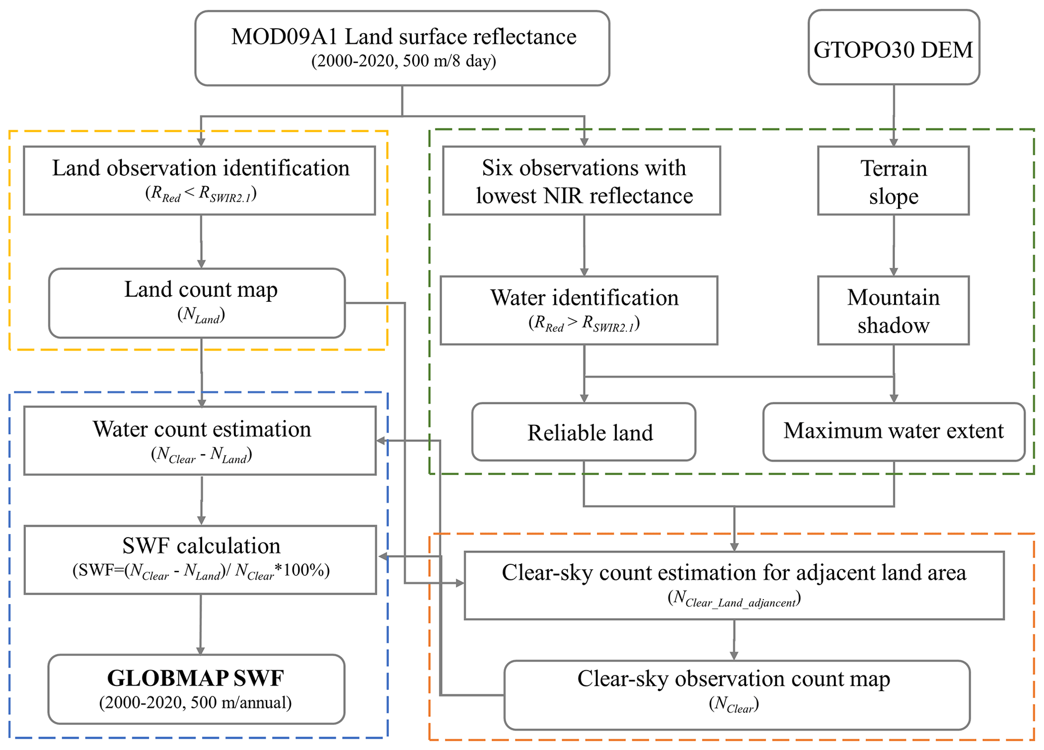
Figure 1 Workflow of the method for generating the GLOBMAP surface water cover frequency dataset.

Firstly, the number of clear-sky land observations during a whole year (N_Land) was counted for each pixel from the MOD09A1 annual land surface reflectance series. The land observations were separated from water and cloud using the reflectance in the red band (R_Red) and SWIR band with a wavelength of 2.1 µm (R_SWIR2.1). Those pixels with R_Red<R_SWIR2.1 were labeled as land. Since R_Red is generally higher than R_SWIR2.1 for water, cloud and snow/ice, the land observations can be reliably identified without the help of cloud masks.

Then, the annual maximum surface water extent was determined from the six observations with the lowest NIR reflectance during a specific year. Water generally has low reflectance in the NIR band (R_NIR), while the presence of cloud and ice/snow would significantly increase the R_NIR. Thus, observations with the lowest R_NIR should be inclined to the clear-sky inundated observation, while the cloud and ice/snow pixels could be excluded reliably. Here, six observations with the lowest R_NIR in a year were selected by weighing available valid observations and possible noise observations, such as shadows, burned areas and occasional water cover. These six observations were assumed to be clear-sky observations, and water observations among them were determined using the criterion of R_Red>R_SWIR2.1. Those pixels with water count ≤1 were identified as reliable land. To exclude possible residual shadows, burned areas and occasional water cover, all pixels with water count ≥3 were used to create the maximum surface water extent map for the specific year. The mountain shadow was excluded using the criterion that the terrain slope derived from DEM >30^∘.

The number of clear-sky observations over the maximum surface water extent (N_Clear) was estimated from the count of clear-sky observations of its adjacent reliable land pixels. Here, clear-sky observation refers to the valid MOD09A1 observation that is not covered with clouds and snow/ice. The coverage of clouds is usually similar for land and water bodies in a small area. This study assumes that the number of clear-sky observations over the water bodies (N_Clear) is the same as that over adjacent land areas (N_{Clear_Land_adjacent}). Here, for each pixel in the maximum surface water extent, 100 spatial nearest reliable land pixels were selected. The count of clear-sky observations for those reliable land pixels is equal to N_Land since all clear-sky observations should be land for reliable land pixels. Then, the N_{Clear_Land_adjacent} was estimated by averaging the N_Land values for the selected 100 nearest reliable land pixels, and the N_Clear was set to equal to the estimated N_{Clear_Land_adjacent}.

Finally, the number of water observations (N_Water) was calculated for the pixels within the range of the maximum surface water extent by subtracting the land observation count (N_Land) from the count of all clear-sky observations (N_Clear). And the SWF was calculated by the water count divided by the count of all clear-sky observations within a year (Eq. 1). Those pixels with N_Land of zero should be covered by water during the whole year, and their SWF values were equal to 100 %, while those pixels with N_Land equal to N_Clear should be permanent land, and their SWF values were equal to 0 %. For large inland water bodies, the adjacent reliable land pixels that were used to estimate N_Clear over the maximum surface water extent may be far away from the water pixels, which may result in uncertainties in N_Clear estimation of water pixels and the SWF consequently. Here, the SWF was set to 100 % for those pixels with N_Land less than a count of 15 for the global largest 100 inland water bodies excluding rivers and water bodies with great seasonal variation in water extent to reduce the influences of uncertainty in N_Clear on the SWF dataset.

$$\begin{array}{}\text{(1)}& \text{SWF}={\displaystyle \frac{N_{\mathrm{Clear}}-N_{\mathrm{Land}}}{N_{\mathrm{Clear}}}}\times \mathrm{100}\mathit{\%}\end{array}$$

Several post-processing procedures were then implemented to the generated SWF maps. The water bodies with an area less than 2×2 pixels were removed to reduce the influence of noise. The oceans were delineated using the ocean label in the state QA flags of MOD09A1 products. The flag of MOD09A1 was used as the initial ocean flag. Those pixels detected as land by the proposed method were labeled as land, and those water pixels between the land and the ocean flagged by MOD09A1 were labeled as ocean. For water bodies that were not marked as oceans in the state flag of MOD09A1, we extended the land boundary toward the water. If the extended land boundaries meet with each other, the water bodies were labeled as inland waters; if the extended land boundaries meet the ocean pixels, the adjacent water pixels were labeled as ocean.

3.2 Validation and inter-comparison with other products

The estimation results were validated with the SWF maps extracted from Sentinel-1 SAR observations in the eight regions (Sect. 2.4). The spatial distribution of our results was compared with the Sentinel-1 results. And the Sentinel-1 SWF maps were resampled to 500 m resolution by averaging the valid SWF estimations from Sentinel-1 data within the MODIS 500 m grid and then compared with GLOBMAP SWF maps pixel by pixel. The root mean standard error (RMSE), absolute mean difference (MAE) and coefficient of determination (R²) were estimated to evaluate the accuracy of GLOBMAP SWF maps.

The estimation results were also compared with the GSWCD and ISWDC products that derived from MODIS observations as well as GSW and GLAD products that derived from Landsat data for characterizing the seasonal variation of surface water. The surface water maps of the five datasets were demonstrated in three lake regions as examples to evaluate their performance in unfrozen water, frozen water and saline lakes, as well as the presence of clouds and bright surfaces. These include Taihu Lake in eastern China (30.62–31.78^∘ N, 119.66–120.82^∘ E), lakes in the northeastern Tibetan Plateau (34.48–36.10^∘ N, 89.71–91.53^∘ E) and Qarhan Salt Lake in the southern Qaidam Basin in northwestern China (36.56–37.24^∘ N, 94.48–96.08^∘ E).

4 Results

4.1 Distribution of global surface water cover frequency

The estimated global SWF map in 2020 is illustrated in Fig. 2a to describe the temporal coverage of inland surface water. The maximum extent, minimum extent (permanent surface water) and intermittent surface water extent are also shown in Fig. 2b–d to characterize the different status of inland water bodies. The intermittent surface water refers to the areas covered by water for part of a year. Some lakes freeze for part of the year. Since snow and ice observations are excluded in estimation of the SWF in the proposed method, the observations in unfrozen periods are used to estimate the surface water cover frequency for the year. If area is underwater for part of the observation period (i.e., the unfrozen period), it is considered to be the intermittent surface water, while if water is present throughout the unfrozen period, the water body is considered to be a permanent surface water. Considering possible uncertainty of the algorithm and quality of satellite observations, here we use SWF ≥10 % for identification of the maximum water extent, SWF ≥90 % for the minimum water extent identification and 10 % ≤ SWF < 90 % for intermittent water identification. For visualization, the SWF was aggregated to 10×10 km grids by averaging all valid SWF values in each grid.

In 2020, the area of the maximum extent of global surface water is 3.38×10⁶ km², of which the permanent surface water (the minimum extent) is 1.83×10⁶ km², and the intermittent surface water is 1.55×10⁶ km². About 46 % of the global total surface water cover (the maximum extent) is intermittent water, which demonstrates the remarkable seasonal dynamics of inland water cover. Compared with the global high-resolution surface water datasets of GSW (Pekel et al., 2016), GLAD (Pickens et al., 2020) and the Global 3 arc-second Water Body Map (G3WBM) (Yamazaki et al., 2015) derived from multi-temporal Landsat images, our estimation results extract less permanent surface water (2.78, 2.93 and 3.25×10⁶ km² for GSW, GLAD and G3WBM respectively) and the maximum surface water (4.46 and 4.82×10⁶ km² for GSW and GLAD respectively). This may be related to the limited spatial resolution of MODIS and post-processing of the dataset, which makes GLOBMAP SWF dataset able to detect inland water body larger than 1 km × 1 km open to the sky, including fresh and salt water. More intermittent surface water is captured compared with the three high-resolution datasets (0.81, 0.74 and 0.49×10⁶ km² for GSW, GLAD and G3WBM respectively) with the aid of frequent MODIS observations to separate the seasonal and permanent water bodies. The inland water bodies are widely distributed across the globe except for the deserts and permanent snow-/ice-covered areas. They are mainly concentrated in midlatitudes to high latitudes of the Northern Hemisphere, such as the northeast of North America, northwest of Europe, north of Russia and the Tibetan Plateau. About 67 % of the maximum surface water is distributed above 35^∘ N, and this percentage reaches 79 % and 54 % for the permanent surface water and intermittent surface water, respectively. The permanent surface water cover is concentrated in the lake areas, such as the Great Lakes in North America, Arctic lakes and lakes in the Tibetan Plateau. The intermittent surface water is widely distributed across the globe, especially in the high latitudes of the Northern Hemisphere, which may be related to the seasonal melting of permafrost. It is also scattered in Africa, Australia, the Pacific Islands and south parts of Eurasia and North America, which may be related to the notable seasonal variations in precipitation.

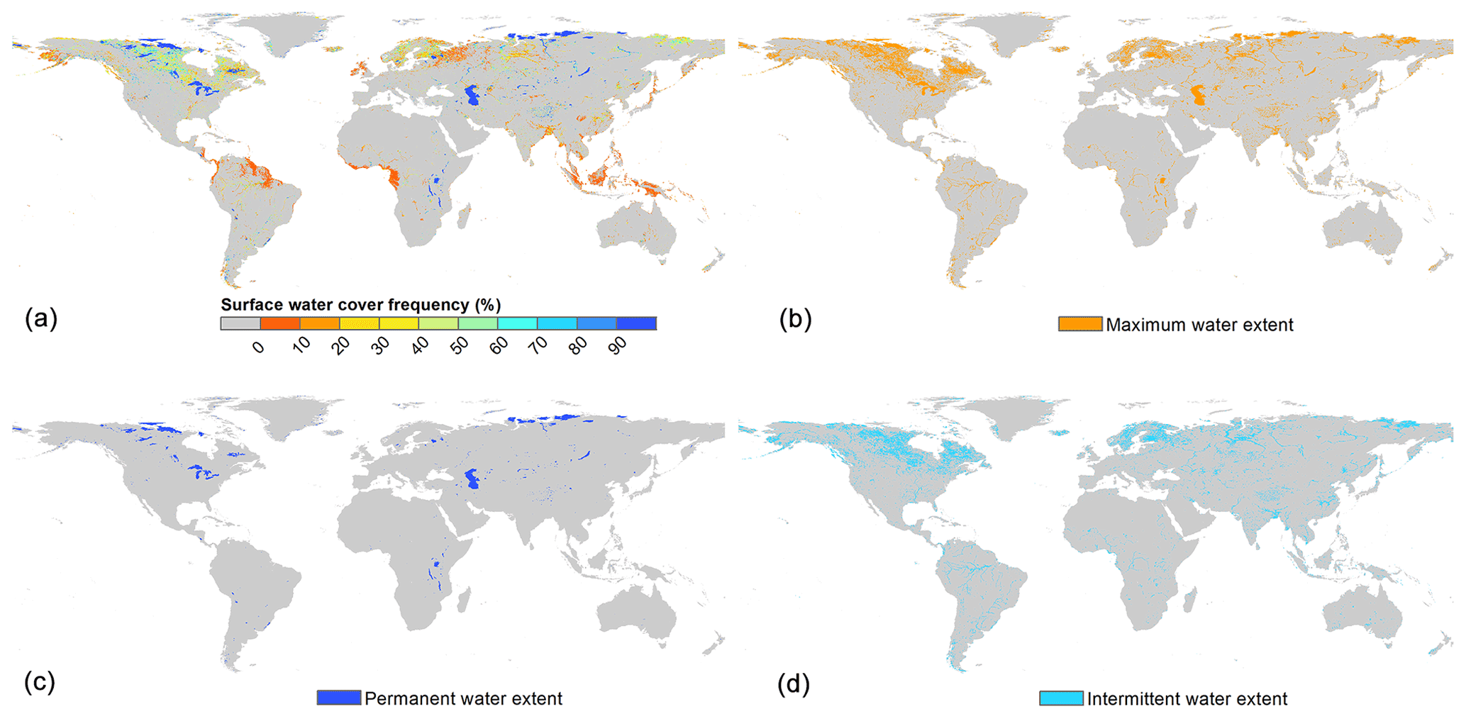
Figure 2 Global distribution of surface water cover frequency in 2020. (a) Global SWF map, (b) the maximum surface water extent, (c) the permanent surface water extent and (d) the intermittent surface water extent. The SWF was aggregated to 10×10 km grids by averaging the valid SWF in each grid for visualization.

4.2 Comparison with existing surface water datasets

The performance of our estimates was evaluated for unfrozen water, frozen water and saline lakes and compared with the surface water datasets of GLAD, GSW, GSWCD and ISWDC. The effects of clouds and bright surfaces were also evaluated. The comparison was performed in three regions as examples, including Taihu Lake in eastern China, lakes in the northeastern Tibetan Plateau and Qarhan Salt Lake in the southern Qaidam Basin.

The performance of unfrozen water and the effects of clouds were evaluated in the Taihu Lake region, the third largest freshwater lake in China. It is located in the subtropical East Asian monsoon region, where clouds frequently occur in summer. Since the average water temperature of Taihu Lake in January is 4 ^∘C, water rarely freezes in winter, with only a little thin ice with a thickness of 1–2 cm in the bay or lee shore. Figure 3 shows the distribution of GLOBMAP SWF, annual water percent dataset of GLAD, seasonality dataset of GSW and the surface water extent map of GSWCD and ISDWC products in January (DOY001) and July (DOY200) in 2015. A Google Earth high-resolution image is presented for reference (Fig. 3a). The results show that the spatial pattern of our estimates is in good agreement with that of the GLAD and GSW. The GLOBMAP SWF reaches 100 % in Taihu Lake and surrounding lakes, indicating that our algorithm successfully extracts the distribution of unfrozen water and reduces the influence of clouds in this region (Fig. 3b). The two Landsat-based products capture more small lakes and narrow rivers with their fine spatial resolution, but the water occurrence of some areas in the northwest part of the Taihu Lake is underestimated, which is probably due to frequent clouds. The surface water maps of GSWCD are generally consistent with our estimation results, GLAD and GSW, suggesting that the interpolation algorithm of GSWCD successfully reconstructs the water cover series in this area. Many lake areas are not identified in the ISDWC maps especially for July (Fig. 3h), which indicates that surface water cover may be underestimated in this dataset due to clouds. Seasonal water cover is observed in our estimates with SWF lower than 30 % in the south and east of Taihu Lake. These intermittent water cover may be related to the seasonal irrigation of paddy rice that is widely planted in this area.

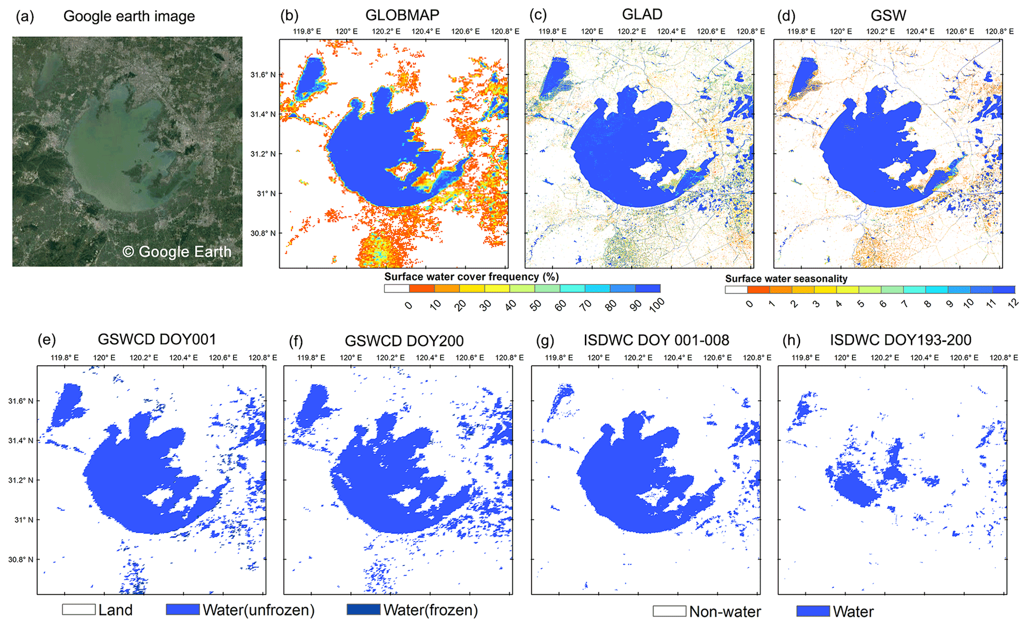
Figure 3 Comparison of surface water map of GLOBMAP SWF, GLAD, GSW, GSWCD and ISDWC in frequently cloud-covered areas around Taihu Lake in eastern China (30.62–31.78^∘ N, 119.66–120.82^∘ E) in 2015. (a) Google Earth high-resolution image (from Google Earth), (b) GLOBMAP surface water cover frequency, (c) GLAD annual water percent and (d) GSW seasonality (source: EC JRC/Google). Surface water extent of GSWCD in (e) DOY001 and (f) DOY200 in 2015 and surface water extent of ISDWC in (g) DOY001–008 and (h) DOY193–200 in 2015.

The performance of frozen water and impact of bright surfaces were compared in lakes in the northeast part of the Tibetan Plateau (Fig. 4). Several lakes are located in this barren area. The altitude reaches around 5000 m, and these lakes are frozen in winter due to extreme cold weather. The GLOBMAP SWF map captures the distribution of lakes in Google Earth images, with the SWF reaching 100 % in the lake areas (Fig. 4b). GLAD and GSW show similar spatial extent of lakes with GLOBMAP, but GLAD seems to underestimate the water occurrence in this region. The surface water cover maps of GSWCD and ISDWC products in July are consistent with our estimation results and Google Earth imagery (Fig. 4f and h). But when it comes to winter in January, some frozen water cover is undetected for the GSWCD product (red circles in Fig. 4e), and many barren land pixels are confused with frozen water. This may be related to the similar high reflectivity in the visible band and low land surface temperature for frozen water and barren land in winter. The ISDWC product fails to detect the lakes in this area in DOY001–008 in 2015 due to cloud contamination (Fig. 4g).

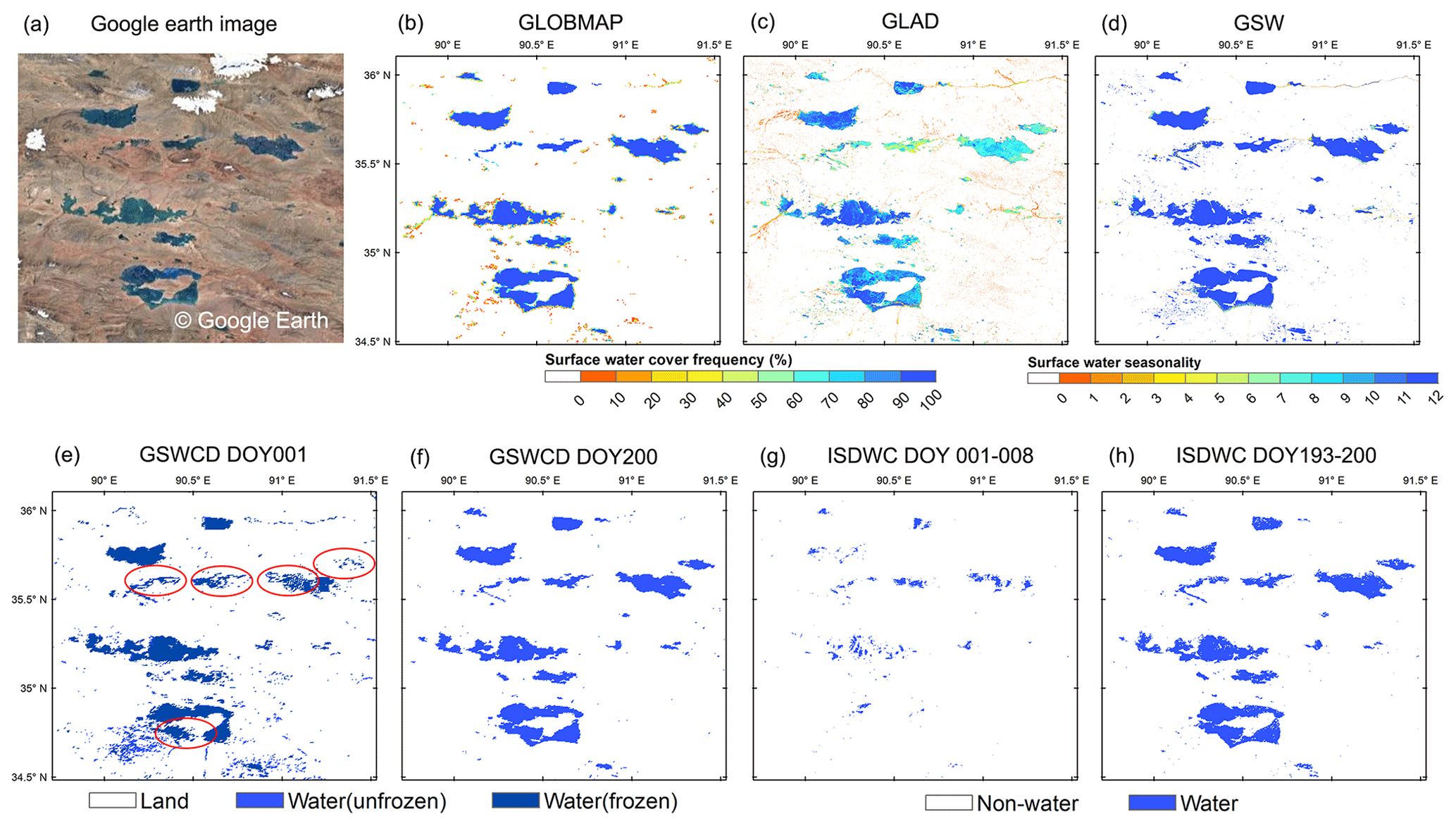
Figure 4 Comparison of surface water map of GLOBMAP SWF, GLAD, GSW, GSWCD and ISDWC for frozen lakes over bright surface in the northeastern Tibetan Plateau (34.48–36.10^∘ N, 89.71–91.53^∘ E) in 2015. (a) Google Earth high-resolution image (from Google Earth), (b) GLOBMAP surface water cover frequency map; (c) GLAD annual water percent and (d) GSW seasonality (source: EC JRC/Google). Surface water extent of GSWCD in (e) DOY001 and (f) DOY200 in 2015 and surface water extent of ISDWC in (g) DOY001–008 and (h) DOY193–200 in 2015.

Figure 5 shows the comparison results of Qarhan Salt Lake, which is located in the Qaidam Basin on the northwestern part of the Tibetan Plateau. As the largest saline lake in China, the lake is rich in inorganic salts such as sodium chloride, potassium chloride and magnesium chloride. Corresponding to the high-resolution image of Google Earth (Fig. 5a), our estimation results, GLAD and GSW successfully extract the distribution of the saline lake. The estimated SWF is approximately 100 % in the lake areas (Fig. 5b), and the derived saline lake map agrees well with the high-resolution images for the four subregions shown by the red rectangles in Fig. 5a (the third row in Fig. 5). GLAD and GSW show more spatial details of the salt lakes. The GSWCD product identifies the majority of the lake, but some lake areas in southern and western parts are missed (red circles in Fig. 5f). Although clear-sky observations were obtained in this area during DOY001–008 and DOY193–200 in 2015 according to MOD09A1 data, many salt water areas are missed in the ISDWC product (red circles in Fig. 5g and h), indicating that the extent of saline lakes may be underestimated in this dataset. Additionally, our estimates also capture the signals of the endorheic Golmud River that flows into the southeast of the saline lake (subregion 2 in Google Earth image).

Figure 5 Comparison of surface water map of GLOBMAP SWF, GLAD, GSW, GSWCD and ISDWC for Qarhan Salt Lake in the southern Qaidam Basin in northwestern China (36.56–37.24^∘ N, 94.48–96.08^∘ E) in 2015. (a) Google Earth high-resolution image (from Google Earth), (b) GLOBMAP surface water cover frequency, (c) GLAD annual water percent and (d) GSW seasonality (source: EC JRC/Google). Surface water extent of GSWCD in (e) DOY001 and (f) DOY200 in 2015 and surface water extent of ISDWC in (g) DOY001–008 and (h) DOY193–200 in 2015. The last row shows the Google Earth high-resolution images for the four subregions shown with the red circles in Fig. 6a (from Google Earth).

4.3 Validation

The accuracy of GLOBMAP SWF dataset was assessed with the 10 m resolution SWF maps extracted from Sentinel-1 SAR data in eight regions that cover lakes, rivers and wetlands. Figure 6 presents the SWF maps of our results and Sentinel-1 as well as the linear regression results of the two datasets.

The surface water extent of GLOMAP SWF is generally consistent with that of Sentinel-1 in these regions, while Sentinel-1 SWF describes more small water bodies and narrow rivers with its high-spatial-resolution observations. Good positive correlation is observed for SWF maps between our estimates and Sentinel-1 results, with R² up to above 0.75 for most regions except for lakes in western Russia (0.46). For the lakes that are mainly covered by permanent surface water in the middle and low latitudes without frequent cloud covers, such as the Lake Albert in the Democratic Republic of the Congo and Uganda, Lake Maggiore in Italy and Lake Wakatipu in New Zealand, the SWF maps of GLOBMAP and Sentinel-1 agree well, with the RMSE ranging from 7.24 % to 13.20 % and MAE from 2.07 % to 2.45 %. For Lake Maggiore that is surrounded by mountains, most of the water extent was extracted compared with the Sentinel-1 results. The performance of the dataset may be affected by frequent cloud cover in tropical regions. For Lake Mai-Ndombe in the southwestern part of the Congo Basin, our dataset can characterize the spatial extent of the lake, but the SWF may be underestimated compared with the Sentinel-1 results, and the RMSE and MAE are increased to 11.28 % and 3.80 % respectively, which may be due to the lack of clear-sky observations in this tropic region. In the western Amazon, both the two SWF maps show widespread seasonal water cover in the Amazon River and permanent water cover in the Taparus River, with an RMSE and MAE of 7.93 % and 2.24 %, respectively. Our estimation results present scattered detection with SWF <10 % in the middle and southern parts of the image, which may also be related to the frequent occurrence of clouds and rain. For the wetlands in western Bangladesh, widespread intermittent water cover and complex surface conditions make it challenging to extract the SWF. Our results generally agree well with the Sentinel-1 SWF map in this region, both showing higher inundation frequency in the northern and middle parts of the wetlands than in the southern part and margins, and the RMSE and MAE are still within 10.8 % and 7.2 %. For lakes in high latitudes, including Lake Winnipegosis and lakes in western Russia, the dataset captures the distribution of large water bodies but may underestimate scattered small lakes in these regions due to the coarse resolution of MODIS data, which makes the RMSE and MAE increase to 16.22 %–22.62 % and 6.17 %–7.04 %, respectively. The comparison indicates that our dataset can also provide reasonable estimates for intermittent inland water bodies, and it is more reliable for large water bodies with less seasonal water cover and clouds.

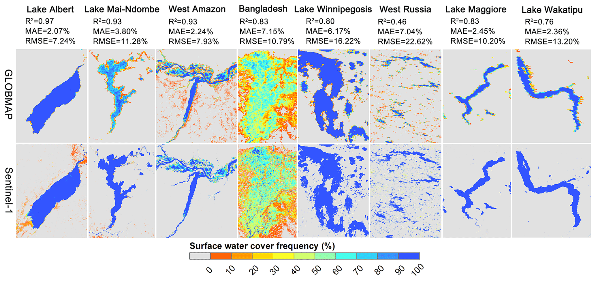
Figure 6 Comparison of GLOBMAP SWF against SWF maps derived from Sentinel-1 in eight regions. These include Lake Albert in the Democratic Republic of the Congo and Uganda (30.98^∘ E, 1.74^∘ N), Lake Mai-Ndombe in western Democratic Republic of the Congo (18.32^∘ E, 2.07^∘ S), the Amazon River and Taparus River in western Amazon in Brazil (54.87^∘ W, 2.16^∘ S), wetlands in western Bangladesh (91.12^∘ E, 24.65^∘ N), Lake Winnipegosis in Canada (99.91^∘ W, 52.61^∘ N), lakes in western Russia (31.00^∘ E, 64.10^∘ N), Lake Maggiore in Italy (8.65^∘ E, 45.90^∘ N) and Lake Wakatipu in New Zealand (168.55^∘ E, 45.10^∘ S). The linear regression results are presented at the top of the figure.

4.4 Interannual variation and change trend of global surface water

The interannual variation and change trend of global maximum, minimum and intermittent surface water were analyzed using the GLOBMAP SWF dataset from 2001 to 2020. Since the MODIS data are incomplete in 2000, the results of 2000 were not used in this analysis. Figure 7 shows interannual variation of the area of global inland water bodies with different inundation frequencies. During the past 2 decades, the average area of global maximum surface water (SWF ≥10 %) is $\mathrm{3.57}\pm \mathrm{0.10}\times {\mathrm{10}}^{\mathrm{6}}$ km², with the largest area of 3.72×10⁶ km² in 2008 and the smallest area of 3.38×10⁶ km² in 2016. The average area of the minimum surface water (permanent surface water, SWF ≥90 %) is $\mathrm{1.89}\pm \mathrm{0.03}\times {\mathrm{10}}^{\mathrm{6}}$ km², which is 53 % of the area of maximum water extent. The permanent water reached the largest extent of 1.95×10⁶ km² in 2001 and the smallest extent of 1.83 km² in 2016. The average area of global intermittent water (10 % ≤ SWF < 90 %) is $\mathrm{1.68}\pm \mathrm{0.08}\times {\mathrm{10}}^{\mathrm{6}}$ km², accounting for 47 % of the maximum water area. Among them, about 79 % of intermittent water occurred in less than half a year (10 % ≤ SWF < 50 %).

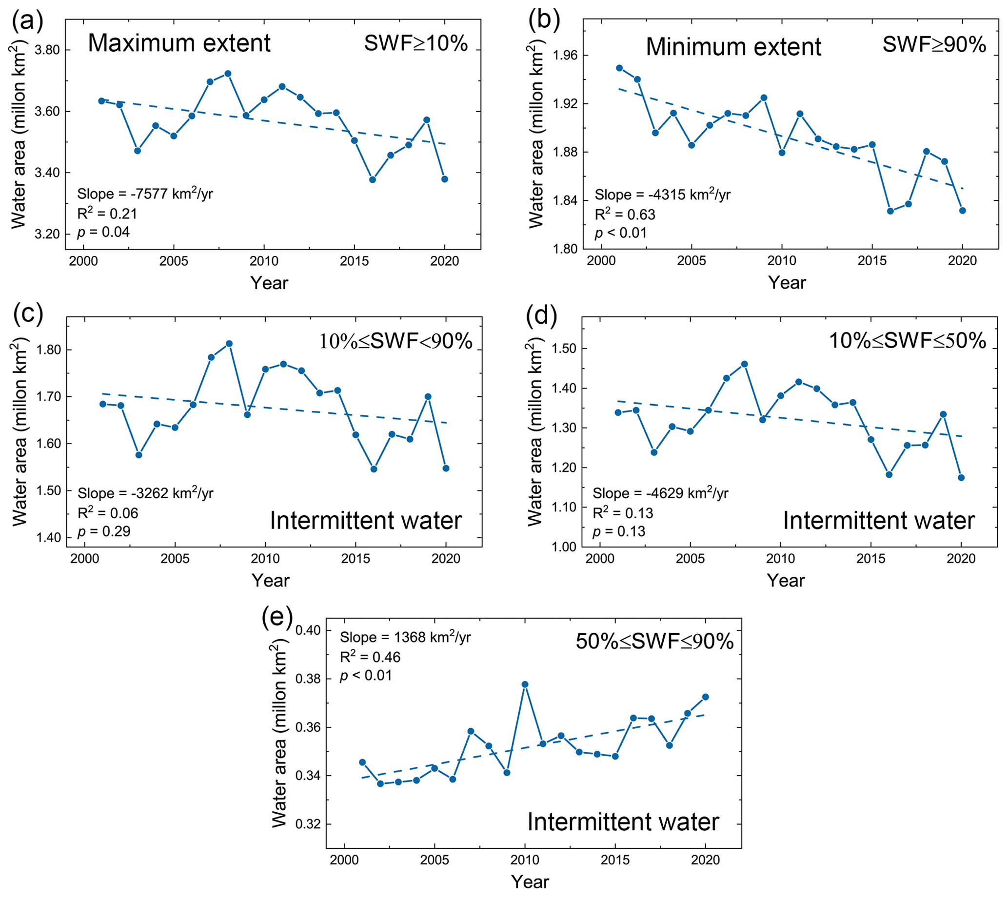
Figure 7 Interannual variation of the area of global surface water with different inundation frequency from 2001 to 2020. (a) Areas of the maximum surface water extent with SWF ≥ 10 %. (b) Areas of the minimum surface water extent with SWF ≥ 90 %. Areas of the intermittent surface water extent with (c) 10 % ≤ SWF < 90 %, (d) 10 % ≤ SWF < 50 % and (e) 50 % ≤ SWF < 90 %.

A decreasing trend is observed for the area of global maximum and minimum surface water since 2001. The maximum water extent shrank at a rate of −7577 km² yr⁻¹ (p=0.04) during 2001–2020, with the downward trend mainly occurring after 2012 (Fig. 7a). The area of permanent surface water has been decreasing continuously since 2001 at a rate of −4315 km² yr⁻¹ (p<0.01) (Fig. 7b). The intermittent surface water also shows an insignificant weak decreasing trend (−3262 km² yr⁻¹, p=0.29). The intermittent surface water was divided up into two parts based on the value of SWF – intermittent water cover with 10 % ≤ SWF < 50 % and that with 50 % ≤ SWF < 90 % – and the areas were then calculated for these two types separately (Fig. 7d and e). The results show that the area of intermittent surface water with SWF less than 50 % also showed a decreasing trend (−4629 km² yr⁻¹, p=0.13) like the maximum water extent, indicating that the extent of global surface water in the wet season was shrinking. In contrast, an increasing trend is observed for the area of intermittent water with SWF above 50 % (1368 km² yr⁻¹, p<0.01), indicating that the temporal coverage period of some permanent water bodies was reduced but still longer than half a year.

A linear trend of SWF was mapped to demonstrate the monotonic changes of surface water inundation frequency during 2001–2020. For visualization, the trend maps were aggregated to 10 km resolution and selected to display the fraction of positive slopes or negative slopes (p<0.05), whichever is larger in each 10 km grid, to represent the main monotonic change type of surface water (Fig. 8a). Grids with a dominantly positive (negative) slope were labeled as inundation frequency increasing (decreasing) areas (positive (negative) fraction). Similarly, we compared the average rate of positive slopes and negative slopes within each 10 km grid, and chose the faster change rate to represent the intensity of surface water changes (Fig. 8b). Grids with positive (negative) slope rate mean that the water occurrence is increasing (decreasing) rapidly. The results show notable changes of water cover extent in the high latitudes of the Northern Hemisphere. In the Arctic, there are more expanded lakes in the south, while the shrinking lakes are concentrated in the north, especially in the northern Arctic regions of Russia and Canada. This is consistent with the findings of Carroll et al. (2011) in Canada. The SWF has increased rapidly in the northern Tibetan Plateau at a rate of above 1.5 % yr⁻¹ (Fig. 8b), which is consistent with the observed extensive lake expansion and new lakes on the plateau due to increased glacial meltwater and precipitation (Zhang et al., 2017). A similar increase of SWF is also observed in southeastern Siberia, northern India, and central and northeastern parts of North America. In contrast, the inundation frequency has been mainly decreased for water bodies of Central Asia, Southeast Asia and southern China, as well as southern parts of South America.

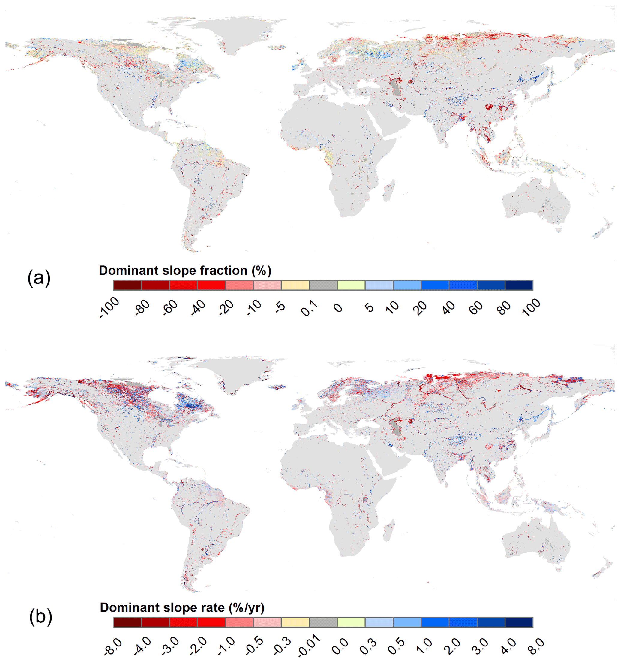
Figure 8 Linear trend of surface water cover frequency during 2001 and 2020. The trend maps were aggregated to 10 km resolution for visualization. (a) Dominant SWF slope fraction (%). The positive (negative) fraction means that the fraction of pixels has increasing (decreasing) SWF (p<0.05) in each 10 km grid, indicating whether the inundation frequency is dominantly increasing (decreasing). (b) Dominant SWF change rate (% yr⁻¹). The positive (negative) slope rate means that the mean linear slope rate of pixels has increasing (decreasing) SWF (p<0.05) in each 10 km grid, whichever is faster, indicating whether the inundation frequency is increasing (decreasing) rapidly. The light grey refers to non-water-covered areas.

4.5 Application examples for surface water dynamic analysis

Two examples are provided in this section to demonstrate the application of GLOBMAP SWF dataset in surface water dynamic analysis. These include the seasonal variation and interannual change of Poyang Lake in southeastern China and global top 10 lakes with the largest seasonal dynamics.

4.5.1 Seasonal and interannual dynamics of Poyang Lake

Analysis of the seasonal and interannual dynamics of inland water body is illustrated for Poyang Lake (28.28–29.89^∘ N, 115.62–117.05^∘ E), which is a large shallow lake located on the south bank of the middle and lower reaches of the Yangtze River. It receives water from five rivers and the surrounding areas and flows into the Yangtze River from the northern lake outlet. The lake shows significant seasonal variations of the water cover area due to the great seasonal fluctuations of regional precipitation and the runoff of the Yangtze River and the five rivers entering the lake, making it challenging to evaluate its interannual change. Figure 9a presents the spatial distribution of GLOBMAP SWF in 2020. The SWF value of most of the lake is ranging from 20 % to 70 %, indicating that the lake is mainly covered by intermittent water. The minimum lake area (SWF ≥ 90 %) during the dry season of 2020 is 545 km², while the maximum area (SWF ≥ 10 %) during the flood season reaches more than 7.4 times the former (4062 km²). Figure 9b shows the interannual series of water cover areas with different inundation frequencies. The maximum lake area shows remarkable fluctuation among years. The area of the maximum lake extent exceeded 4900 km² in 2002, 2010 and 2012, while it reduced to below 4000 km² in 2004, 2007, 2008, 2013–2015, 2017 and 2018, and the smallest area was only 3055 km² in 2011. The maximum lake area is closely related to the amount of water entering the lake during the flood season. The Poyang Lake basin and the Yangtze River basin are located in the East Asia monsoon region. The precipitation is mainly concentrated in summer and has significant interannual fluctuations, resulting in notable interannual variations of the lake area in the flood season. The interannual variation of lake area decreases gradually with the increase of SWF and reaches the lowest for the minimum lake extent that occurred during the dry season. Precipitation in the dry season (winter) is much less frequent and less affected by abnormal climate, which may reduce the year-by-year fluctuation of the lake area in the dry season consequently. In 2003, the permanent lake area decreased abruptly from 947 to 512 km² and then remained at a low value, with the area ranging from 500 to 660 km² for most years after 2003, which coincides with the time of the impoundment of the Three Gorges Dam in 2003. These results are consistent with the decline of the annual minimum inundation area (Feng et al., 2012) and the rapid increase of wetland vegetation coverage in this region after 2002 (Han et al., 2015). The available count of clear-sky observations was averaged over the maximum surface water extent in the Poyang Lake region for each year during 2001–2020 (purple line in Fig. 9b). The average N_Clear was between 33 and 39 during this 20-year period. Correlation was observed between the area of maximum surface water extent and the N_Clear. More clear-sky observations mean less precipitation, which may lead to a smaller lake area, while fewer clear-sky observations mean more precipitation, and the lake area should be larger. However, the two variables do not correspond exactly, which indicates that the maximum surface water area does not depend on the available number of clear-sky observations. The minimum surface water area shows no obvious correlation with N_Clear, and its interannual fluctuation should be related to precipitation and the amount of water entering the lake in the dry season.

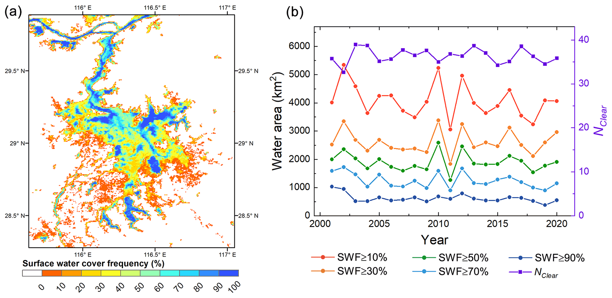
Figure 9 The seasonal variation and interannual change of surface water cover of Poyang Lake (28.28–29.89^∘ N, 115.62–117.05^∘ E). (a) The GLOBMAP SWF map in 2020. (b) The interannual variation of the area of Poyang Lake with different inundation frequency and average value of the count of available clear-sky observations (N_clear) over the maximum surface water extent from 2001 to 2020.

4.5.2 Top 10 lakes with significant seasonal variation

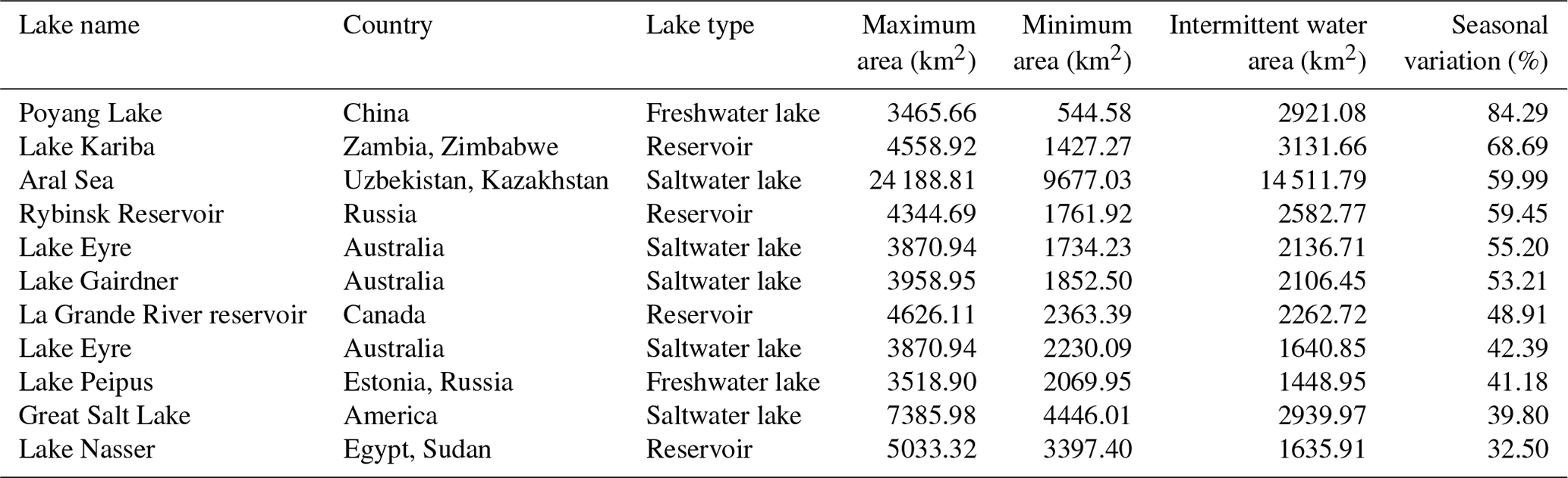
The 10 lakes with the largest seasonal variation in 2020 were identified to illustrate the seasonal fluctuation of inland open surface water. Seasonal variation was evaluated with the proportion of the intermittent water area to the maximum water area in this year. All lakes whose maximum water cover extent >3000 km² were ranked with their seasonal variation, and the top 10 lakes are listed in Table 1.

The results show that the intermittent water area of these 10 lakes accounts for more than 30 % of the maximum water area. Poyang Lake in eastern China presents the largest seasonal fluctuation, with the seasonal variation reaching 84.29 %. These 10 lakes can be divided into three types: two natural freshwater lakes, four natural saltwater lakes and four reservoirs. Among them, natural freshwater lakes include Poyang Lake and Lake Peipus. Both lakes are shallow in depth, and the relief of the bottom and surrounding area is flat, which means the water area may rise dramatically in the flood season and fall during the dry season. For example, the shores of the Lake Peipus are usually flooded in the spring, with the flooding area reaching up to 1000 km². Saltwater lakes include the Aral Sea, Lake Gairdner, Lake Eyre and Great Salt Lake. These lakes are all endorheic lakes that are located in the arid regions of Central Asia, Australia and North America. Similar to the two freshwater lakes, the water depth is also shallow for these four saltwater lakes. In the wet season, the river runoff and local precipitation make the lake extent expand, while in the dry season, the lakes shrink significantly due to the strong evaporation. Four reservoirs, including Lake Kariba, Rybinsk Reservoir, La Grande River reservoir and Lake Nasser, are also listed in the top 10 lakes. The notable seasonal fluctuation of reservoir area should be related to artificial impoundment and drainage of the reservoir dam.

Table 1 Global top 10 lakes with the largest seasonal variation in 2020.

5 Discussions

It is challenging to capture the interannual variation and change trend of inland water bodies due to their significant seasonal variations. The extent of surface water usually varies during a year due to the seasonal cycle of precipitation and evaporation, and it may also change abruptly due to large amount of rainfall and human activities, such as reservoir construction, mining and irrigation (Tao et al., 2015). The timing of seasonal variation in surface water extent often varies among years due to interannual shifts of the timing of precipitation and human activities. Thus, it may be incomparable for the snapshot of surface water acquired at the same period or during a specific period such as the high-water period that is usually analyzed (e.g., in summer or wet season), which would misinterpret its interannual change and long-term trend. Here, we generated a global surface water cover frequency dataset from high-frequency MODIS data to characterize the seasonal variation and interannual change of inland water bodies. This dataset simplifies the multi-period water cover maps to the percentage of period that a pixel is covered by water in a year. It can characterize the temporal coverage frequency of surface water, which is suitable to represent the spatiotemporal characteristics of intermittent waters. The extent of maximum, minimum and different inundation frequency of surface water can be estimated from the dataset without the influence of the occurrence period, which helps to avoid misidentifying seasonal changes in water cover as interannual changes.

This paper developed a method for surface water extraction from a new perspective, which estimates the SWF indirectly by identifying land observations in annual observation series to reduce the influence of clouds, snow/ice and variable characteristics of water body and surface background. Water generally absorbs more solar radiation in spectral bands with longer wavelengths, resulting in the greater reflectivity of visible bands than that of NIR and SWIR bands. This spectral contrast has been widely used to extract surface water extent directly (e.g., GSWCD), and several spectral indices have been proposed for surface water extraction with the reflectance in the visible band (usually green) and NIR or SWIR band, such as the Normalized Difference Water Index (NDWI) (McFeeters, 1996) and the Improved Normalized Difference Water Index (MNDWI) (Xu, 2006). To reduce the effects of clouds, the threshold of index is usually set to greater than zero in surface water mapping. When it comes to special water bodies with high reflectivities, such as frozen water, saline lakes and turbid water bodies, the value of these indices may be below the threshold, resulting in misdetection. Additionally, variation of surface background may also result in confusion in water extraction, which has been demonstrated in the misdetection of lakes on the bright surface of the northeastern Tibetan Plateau (Sect. 4.2). These may introduce substantial uncertainties in global water cover mapping with the direct water extraction algorithm. In the generation of global water datasets, it is not only needed to propose good water cover extraction algorithm, but also to consider data quality, noise and applicability of the algorithm in different regions. We found a reliable and robust method to separate land from water, cloud and snow/ice. The R_Red of the former is generally lower than that of R_SWIR, while it is opposite for the latter three. If the SWF values were estimated indirectly by identifying land, the interference of cloud and snow/ice in water identification would be avoided. In this paper, instead of identifying water cover directly, the frequency of surface water cover was estimated by subtracting the count of land observations from the count of total clear-sky observations, which avoids directly distinguishing water from cloud and snow/ice. The annual maximum water surface extent was extracted based on the minimum near-infrared reflectance composition method, which automatically excludes the influence of clouds, ice and snow. Moreover, the land identification method (R_Red<R_SWIR) was applicable for major types of water bodies and surface background and can exclude cloud and snow/ice observations. Through these procedures, the proposed algorithm is ubiquitous for various water bodies and surface background and reduces the interference of cloud and snow/ice, which helps to improve the applicability of our algorithm across the globe.

Several factors may affect the performance of the proposed approach, including clouds, shadows, thawing of snow and ice, and spatial resolution. Clouds can obscure surface water signals in optical remote sensing. They usually occur more frequently during the rainy season, while the clear-sky observations are inclined to occur in the dry season. Since our algorithm uses the percentage of water observations in all clear-sky observations to estimate the water cover frequency within a whole year, the cloud observations that are concentrated in the rainy season are not taken into account, which may lead to underestimation of the SWF (Lake Mai-Ndombe in Fig. 6). The number of available clear-sky snow/ice-free observations in a year (N_Clear) was counted during the period 2001–2020 over global terrestrial surface. There are on average 4285 pixels with N_Clear≤6, accounting for 0.0008 % of the total terrestrial surface pixels (550 215 315) in a year. This percentage is 0.02 % (460 pixels out of total 1 901 338 water pixels) for the inland water bodies. Since the proportion of pixels with extreme sparse clear-sky observation is very small, its influences should be limited at global scale. Figure 10 shows the global map of N_Clear in 2020. Fortunately, N_Clear is generally above 40 in arid and semi-arid areas, where water bodies may show significant season variation in their extent. The low N_Clear values are concentrated in the tropics and subtropics, such as the Gulf of Guinea, the Amazon, the Southeast Asia, and the Sichuan Basin in southwestern China, where N_Clear mostly ranges from 25 to 35. Since surface water generally shows relatively small seasonal changes in the tropics and subtropics, the available clear-sky observations should be able to capture the distribution of surface water. In high latitudes in the Northern Hemisphere, N_Clear is generally reduced to 10–25 due to a long period of snow/ice cover and the polar night in winter. The proposed algorithm excludes snow/ice observations and uses the observations in unfrozen period to estimate the surface water cover frequency. In the glacial areas, such as Greenland and glacial areas of the Tibetan Plateau, N_Clear is less than 10 as snow and ice observations are excluded in the counting of clear-sky observations, but it should have little impact on the dataset due to limited water bodies in these regions. In some areas in the central part of several huge lakes (e.g., Caspian Sea), since they are far away from the land pixels on the shore and their clear-sky observations may be different from that of the adjacent reliable land pixels, N_Clear values are set to fill value to reduce the uncertainties in N_Clear estimation. The SWF of these regions is usually estimated to be 100 %, as its N_land is usually less than 15. The limited number of valid observations is a common problem for optical remote sensing. The MODIS onboard Terra and Aqua satellites observe the Earth's surface every 1 to 2 d. Their dense time series can be acquired to generate more clear-sky observations. Additionally, in the proposed method, all pixels with water count ≥3 among six observations with the lowest NIR reflectance were used to create the maximum surface water extent map. This means that the algorithm can be implemented with three valid observations during a year, which helps to improve the global applicability of the algorithm.

Figure 10 Global map of the number of clear-sky snow/ice-free MOD09A1 observations in 2020.

The mountain shadows were masked using the criterion that the terrain slope derived from DEM data is greater than 30^∘. In areas with complex terrain, this simplification may result in uncertainties of the estimation results. The variation of solar angle along latitudes and seasons was not considered in the slope criteria for shadow estimation, which may cause water that is outside of shadow to be removed in mountainous areas. Here, the DEM data were mainly used to exclude large areas mountain shadows, such as shadows in the margin of the Tibetan Plateau. For mountain shadows with a small range, since the local time when MODIS passes changes among days, the distribution of shadows will change due to different solar and viewing geometry. MOD09A1 selects the best possible observation during an 8 d composition period, and its spatial resolution is coarse (500 m), which helps to reduce the effects of mountain shadows with a small range. It would help to improve the identification of terrain shadows by considering solar angle variation and using fine-resolution DEM data, such as GMTED2010.

In snow-/ice-covered areas, the meltwater on the ice would reduce the reflectivity in the NIR band. This may lead to overestimation of the maximum water area since the six observations with the lowest NIR reflectivity are used to extract the annual maximum water extent. Here, we create the maximum surface water extent map using those pixels with water count no less than 3 to remove possible false detections.

Additionally, the spatial resolution of MODIS may limit the identification for narrow rivers and small water bodies, resulting in underestimation of surface water extent. It is difficult for the dataset to capture small water bodies and the subtle changes of surface water, especially in high latitudes in the Northern Hemisphere, where a large number of small water bodies are located. Satellite data often have certain advantages in terms of temporal or spatial resolution and time coverage, etc., but it is difficult to take into account all of these aspects. MODIS provides daily spectral measurements of the Earth surface since 2000. Its long-term high-frequency observations have unique advantages in monitoring of the seasonal and interannual changes in surface water. High-resolution images such as from Sentinel-1 and Sentinel-2 would help to improve the surface water extraction in these areas.

6 Data availability

The GLOBMAP SWF dataset is available on the Zenodo repository at https://doi.org/10.5281/zenodo.6462883 (Liu and Liu, 2022). The number of MOD09A1 clear-sky snow-/ice-free observations (N_Clear) data is also provided as a quality dataset. The dataset is provided by 296 1200 km × 1200 km tiles at annual temporal and 500 m spatial resolutions in the sinusoidal projection in Geotiff format for each year during 2000–2020. The SWF file is named “GLOBMAPSWF.AYYYY001.hHHvVV.V01.tif”, while the N_Clear file is named “GLOBMAPClearCount.AYYYY001.hHHvVV.V01.tif”, where “YYYY” refers to the year of the file, and “HH” and “VV” explain the number of tiles that are the same as the MODIS standard tile. For the SWF dataset, the valid range is 0–100, the scale factor is 1.0 and the unit is percent. For the N_Clear dataset, the valid range is 0–46, and the scale factor is 1.0.

7 Conclusions

In this paper, a global annual surface water cover frequency dataset (GLOBMAP SWF) was generated at 500 m resolution from MODIS land surface reflectance data from 2000 to 2020. The SWF was proposed to quantitatively describe the seasonal dynamics of inland water bodies by estimating the percentage of water cover occurrence in a year. The count of a pixel covered by water was estimated indirectly by subtracting the land observation count from total clear-sky observation count. The SWF was calculated by dividing the water count by the total number of clear-sky observations without the help of cloud masks.

In 2020, the area of global maximum surface water extent is 3.38×10⁶ km², of which the permanent surface water is 1.83×10⁶ km² (54 %), and the intermittent surface water is 1.55×10⁶ km² (46 %). The inland water bodies are mainly concentrated in midlatitudes–high latitudes of the Northern Hemisphere above 35^∘ N. Compared with the high-frequency GSWCD and ISWDC datasets derived from MODIS data, the regional analysis demonstrates that our estimation results show better performances for frozen water and saline lakes; the influence of clouds is successfully reduced, with the estimated SWF reaching 100 % for permanent water bodies in cloud frequently covered regions. And the false detection was also reduced over the bright surface in winter. When compared with the high-resolution GLAD and GSW datasets derived from Landsat data, the generated dataset captures more intermittent surface water, but small water bodies may be underestimated due to the coarse spatial resolution of MODIS. Our estimates are validated with the 10 m resolution SWF maps extracted from Sentinel-1 SAR observations in eight regions that cover lakes, rivers and wetlands. Consistent spatial patterns and good positive correlations are observed between the two results, with the R² up to 0.46–0.97, RMSE ranging from 7.24 % to 22.62 %, and MAE between 2.07 % and 7.15 %. During 2001–2020, a decreasing trend is observed for the area of global maximum (−7577 km² yr⁻¹, p=0.04) and minimum (−4315 km² yr⁻¹, p<0.01) surface water. The intermittent water also showed an insignificant weak decreasing trend (−3262 km² yr⁻¹, p=0.29), while that with SWF above 50 % has been expanding since 2001 (1368 km² yr⁻¹, p<0.01).

The GLOBMAP SWF dataset condenses the seasonal variation of inland water bodies to inundation frequency during a year. It can characterize the spatial distribution of permanent water extent in the dry season and maximum water extent in the rainy season, as well as the distribution of intermittent water and the length of inundation period. The dataset can be used to analyze the interannual variation and change trend of surface water with consideration of its seasonal variation and may guide the scientific management of water resources and the investment in water infrastructures.