the Creative Commons Attribution 4.0 License.
the Creative Commons Attribution 4.0 License.
 | 29 Sep 2022
Streamflow data availability in Europe: a detailed dataset of interpolated flow-duration curves
Simone Persiano
Alessio Pugliese
Alberto Aloe
Jon Olav Skøien
Attilio Castellarin
Alberto Pistocchi
For about 24 000 river basins across Europe, we provide a continuous representation of the streamflow regime in terms of empirical flow-duration curves (FDCs), which are key signatures of the hydrological behaviour of a catchment and are widely used for supporting decisions on water resource management as well as for assessing hydrologic change. In this study, FDCs are estimated by means of the geostatistical procedure termed total negative deviation top-kriging (TNDTK), starting from the empirical FDCs made available by the Joint Research Centre of the European Commission (DG-JRC) for about 3000 discharge measurement stations across Europe. Consistent with previous studies, TNDTK is shown to provide high accuracy for the entire study area, even with different degrees of reliability, which varies significantly over the study area. In order to provide this kind of information site by site, together with the estimated FDCs, for each catchment we provide indicators of the accuracy and reliability of the performed large-scale geostatistical prediction. The dataset is freely available at the PANGAEA open-access library (Data Publisher for Earth & Environmental Science) at https://doi.org/10.1594/PANGAEA.938975 (Persiano et al., 2021b).
- Article
(12297 KB) - Full-text XML
- BibTeX
- EndNote


Over the past decades, the increasing accessibility of global datasets (soil, land cover, morphology, climate characteristics, satellite-based gridded precipitation, etc.) and the ever-expanding computational capabilities have triggered the development of macro-, continental- and global-scale rainfall-runoff simulation models, which are already state of the art (see e.g. Collischonn et al., 2007; de Paiva et al., 2013). Macro-scale models are getting more and more popular and accurate in terms of average performance over large areas; their simulated streamflow series, some of which are open-access and freely distributed, represent a wealth of information for addressing a variety of water problems, such as the streamflow regime prediction in data-scarce regions of the world (Pechlivanidis and Arheimer, 2015) and the implementation of large-scale and transboundary policies for water resource system management or flood-risk mitigation (de Paiva et al., 2013; Sampson et al., 2015; Falter et al., 2016). Due to the impossibility of performing comprehensive calibrations and validations of such models over the whole modelled regions, local performance can be rather diverse (see e.g. de Paiva et al., 2013; Donnelly et al., 2016), depending on several factors, e.g. the quality of macro-scale input data or the ability of the selected conceptual scheme to accurately represent the dominant hydrological processes locally governing the rainfall-runoff transformation (geological and morphological or climatic and micro-climatic factors).
An empirical characterization of the natural streamflow regime over large areas would be a fundamental piece of information for benchmarking the performance of macro-scale models and for assessing their potential locally. This necessity conflicts with the availability and accessibility of streamflow observations, which can be limited even in technologically advanced regions of the world.
In this context, along the lines of the study conducted by Castellarin et al. (2018) for the Danube region, the present study performs a statistical regionalization of streamflow regimes in Europe, compiling a data-driven benchmark dataset for hydrological models as well as a data layer to be made available for broader use. The streamflow regime for each catchment is characterized in terms of a flow-duration curve (FDC), a graphical representation of the frequency (i.e. percentage of time or duration) with which a given streamflow is equalled or exceeded over a historical period of time at a given river basin (see e.g. Vogel and Fennessey, 1994). Providing a simple and compact view of the historical variability of streamflows, from high flows to low flows, an FDC is a key signature of the hydrological behaviour of a catchment: its shape reflects climate conditions and the hydrogeological characteristics (i.e. size, morphology, permeability) of the catchment itself (see e.g. Castellarin, 2014; Westerberg et al., 2016). For this reason, FDCs are routinely used for addressing water resource management problems such as hydropower feasibility studies, classification of streamflow regimes, irrigation planning and management, definition of environmental flows and habitat suitability studies (e.g. Vogel and Fennessey, 1995; Yaeger et al., 2012) as well as for assessing hydrologic change at a river cross section (Kroll et al., 2015; Ceola et al., 2018).
Starting from a compilation of about 3000 discharge measurement stations across Europe, where streamflow indices and empirical period-of-record FDCs (POR FDCs) (i.e. 15 streamflow quantiles) are compiled by the Joint Research Centre of the European Commission (DG-JRC) from the archives of the Global Runoff Data Centre (GRDC), here we perform a geostatistical interpolation of the streamflow regime to provide FDC estimates for a total of 24 148 elementary catchments for the European region. With this aim, high-quality empirical POR FDCs are interpolated over the stream network using the geostatistical procedure termed total negative deviation top-kriging (TNDTK; Pugliese et al., 2014, 2016), which has been shown to provide reliable predictions of continuous FDCs at ungauged locations, overcoming the limit of regression models of modelling streamflow quantiles independently of each other (Pugliese et al., 2016; Castellarin et al., 2018). Also, being a BLUE (i.e. best linear unbiased estimator) procedure, TNDTK was shown to be an effective tool for correcting systematic bias associated with the outcomes of macro-scale rainfall-runoff models (i.e. Pugliese et al., 2018). In line with Castellarin et al. (2018), together with the estimated FDCs, for each elementary catchment we provide indicators of the accuracy and reliability of the performed large-scale geostatistical prediction.
2.1 Source data and screening
The present study uses a database compiled by the DG-JRC, consisting of 3138 stream gauges across Europe. For the catchment upstream from each gauged station, streamflow indices and several catchment descriptors are available. Streamflow indices are computed from the streamflow time series observed at each gauge and consist of mean annual flow (MAF, long-term average daily discharge) and 15 streamflow quantiles associated with duration of 1 %, 5 %, 10 %, 20 %, 30 %, 40 %, 50 %, 60 %, 70 %, 75 %, 80 %, 90 %, 95 %, 97 % and 99.7 %. The quality of streamflow data is classified as high and low: high-quality data refer to gauging stations with a precise positioning along the stream that are unique in their elementary sub-basin (i.e. the portion of the basin directly drained by a river stretch, between two confluences, or from the headwater to the first confluence), whereas low-quality data refer to cases in which more stream gauges are present in a single elementary basin, hence potentially being affected by imprecise positioning along the stream (see also Castellarin et al., 2018). In particular, 3004 study catchments are extracted from the original DG-JRC database of 3138 measuring points by consolidating and merging multiple entries (i.e. in case of stream gauge redundancy for a given location, only the highest-quality stream gauge associated with the largest drainage area is retained).
Among the 3004 selected catchments, empirical MAF values observed at high-quality measuring points show a minimum, 1st quartile, median, mean, 3rd quartile and maximum equal to 0.01, 3.03, 9.41, 80.16, 35.38 and 6378.00 m3 s−1, in this order. Consistent with Castellarin et al. (2018), based on the values of MAF standardized by catchment area (i.e. unit mean annual flow, MAF/area) as a function of basin area (see Fig. 1), the 146 measuring points falling outside the interval 0.0015–0.08 m3 s−1 km−2 are regarded as highly discordant and are therefore excluded from further analyses. Among the 2858 retained catchments, Figs. 1 and 2 highlight the predominance of stream gauges with high-quality data (2484) over the low-quality ones (374, mainly concentrated in the area of the Danube region; see Castellarin et al., 2018).

Figure 1Unit mean annual flow (MAF/area) as a function of basin area for the 3004 study catchments. Stream gauges located outside the interval 0.08–0.0015 m3 s−1 km−2 (see horizontal dashed lines) are identified as highly discordant and are removed from the dataset. Blue and red points are associated with high- and low-quality data, respectively.
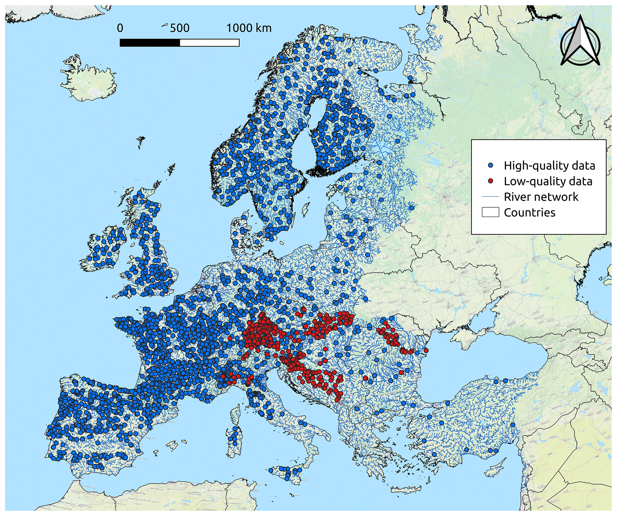
Figure 2Stream gauges (2858) retained from the DG-JRC database. Blue and red points refer to high- and low-quality data, respectively.
Differently from the case study of the Danube region described in Castellarin et al. (2018), for which the analysis was performed twice (first by considering low- and high-quality data combined and then by focusing only on high-quality data), for the European continent we focus only on the 2484 measuring points associated with high-quality data.
Together with the above-mentioned stream gauges, the DG-JRC identifies a layer of 32 960 prediction nodes over the entire European region, for which we perform the prediction of FDCs described herein.
2.2 Methods: geostatistical interpolation
Based on what was performed for the Danube region in Castellarin et al. (2018), FDC predictions at the DG-JRC catchments are obtained by applying the geostatistical procedure named TNDTK (Pugliese et al., 2014, 2016). TNDTK is based on top-kriging (Skøien et al., 2006, 2014), a geostatistical tool which is widely used in the literature for predicting streamflow indices (e.g. low flows; see Castiglioni et al., 2011; Laaha et al., 2014; high flows and floods; see Merz et al., 2008; Archfield et al., 2013; Persiano et al., 2021a), habitat suitability indices (Ceola et al., 2018) and daily streamflow series (Skøien and Blöschl, 2007; de Lavenne et al., 2016; Farmer, 2016) at ungauged river cross sections as linear combinations of the empirical information collected at neighbouring gauging stations by accounting for the catchment size and nesting structure of the stream network. Specifically, TNDTK (Pugliese et al., 2014, 2016) uses top-kriging in an index-flow framework (Castellarin et al., 2004) for predicting the entire FDC at ungauged sites, ensuring its monotonicity. With this aim, as a first step, the dimensionality of the problem is reduced by standardizing the empirical FDC at site x, Ψ(x,d) (where d is a specific duration), for a reference value (e.g. MAF), Q∗(x), to yield a dimensionless FDC, ψ(x,d):
Pugliese et al. (2014) identify an overall point index, named total negative deviation (TND), which effectively summarizes the entire curve. TND is derived by integrating the area between the lower limb of the FDC and the reference streamflow value Q∗(x) (see e.g. Fig. 1 in Pugliese et al., 2014). Even though TND does not capture the portion of the FDC associated with low durations (i.e. high flows), it is very informative on the shape of the FDC that is controlled by climatic, physiographic, and geo-pedological characteristics of the catchment (see Pugliese et al., 2014). Larger TNDs are associated with steeper FDCs (i.e. catchments with rapidly responding runoff processes), while smaller TNDs are associated with less steep FDCs. Therefore, being capable of expressing the hydrological similarity between catchments, TND is used as a regionalized variable to develop site-specific weighting schemes within the TDNTK procedure. The same weights, derived through the solution of the linear kriging system, are used for a batch prediction of the continuous dimensionless FDC, , for the ungauged site x0:
where λj, for , are the weights resulting from the kriging interpolation of TNDs for the n neighbouring gauged catchments, and ψ(xj,d) is the dimensionless empirical FDC at the donor site xj. Equation (2) highlights that the computation of kriging weights depends on n, the number of neighbouring sites on which to base the spatial interpolation.
Once a reliable model (e.g. a regional regression model or kriging model) for predicting Q∗ at the ungauged site x0 (i.e. has been set up for the study region, the prediction of the dimensional FDC, , can be obtained as
For the sake of brevity, this prediction method is referred to as TNDTK. Additional details can be found in Pugliese et al. (2014). TNDTK has been shown to provide reliable predictions of FDCs at ungauged sites over large study areas (Castellarin et al., 2018) and to reliably reconstruct natural FDCs at ungauged sites (Ceola et al., 2018).
3.1 Application of the geostatistical interpolation
In the present study, TNDTK is applied by implementing the R package “rtop” (Skøien et al., 2014). The MAF is chosen as the reference streamflow value Q∗ used for standardizing empirical FDCs across the study region, and empirical TND values are computed for each empirical dimensionless FDC, standardized by local MAF values. It is worth highlighting that, while computing TND values, the durations of interest are transformed into standard normal variates using the meta-Gaussian transformation, which enhances the representation of the right tail of FDCs and therefore better differentiates TND values associated with different empirical curves. Either for MAF or TND interpolations, top-kriging is implemented by following the next steps: (1) the binned sample variogram is calculated, (2) the five-parameter theoretical variogram (i.e. a “modified” exponential model, which combines an exponential model with a fractal model; see details in Skøien et al., 2006) is then regressed against the sample variogram through a weighted least squares (WLS) regression method (Cressie, 1993), and (3) from the theoretical variograms the kriging weights for n=6 neighbouring stream gauges are computed for any prediction location and the streamflow index of interest is predicted at that location. n=6 was set after a preliminary sensitivity analysis which confirmed the results obtained in previous studies (Pugliese et al., 2014, 2016), suggesting that the size of nearest neighbours should be kept limited when interpolating streamflow indices, and TND values in particular. Moreover, differently to what was done for the Danube region in Castellarin et al. (2018), for application to the entire European continent, 300 km is set as the maximum distance from the prediction location within which gauged basins are included for the prediction itself.
In this study, TNDTK is used for predicting long-term FDCs at prediction points located at the outlets of 21 664 elementary catchments (elementary catchment minimum drainage area: 0.01 km2; average drainage area: 172.83 km2; maximum drainage area: 1668.38 km2) located within the European continent. In particular, interpolation is performed only within watersheds including at least one measuring point of the DG-JRC dataset (see the blue area in Fig. 3). Elementary catchments within watersheds where no measuring gauges are present have been excluded from the analysis (see the black area in Fig. 3).
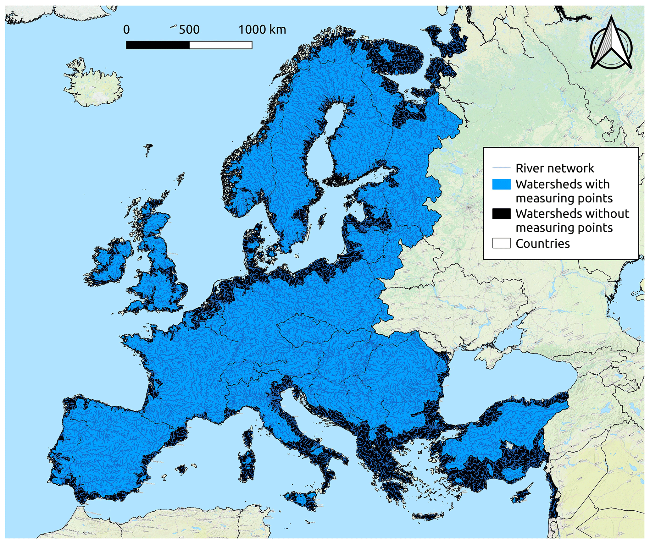
Figure 3Merger of the elementary catchments from the DG-JRC database. Predictions have been performed for elementary catchments within the blue area, while no predictions have been provided for the black area.
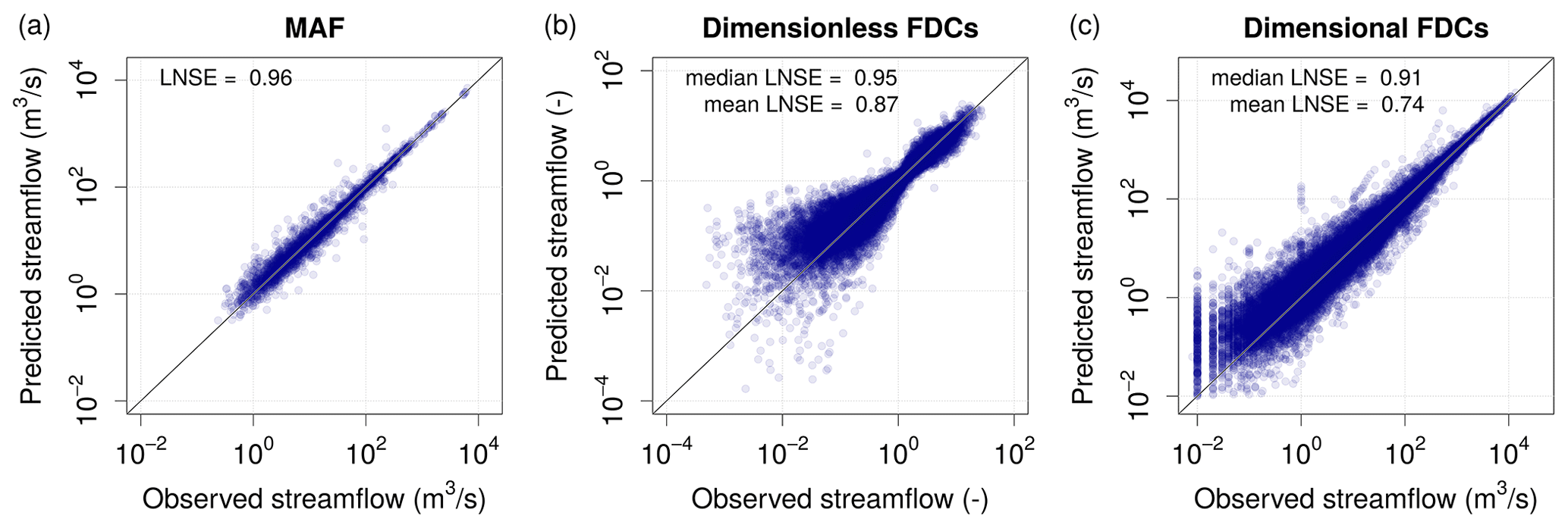
Figure 4Results of the top-kriging interpolation in cross-validation (LOOCV). For (a) MAF, (b) dimensionless FCDs, and (c) dimensional FDCs, empirical (x axes) vs. predicted (y axes) values are reported together with the overall Nash–Sutcliffe efficiency for log-transformed (LNSE) streamflows.
3.2 Cross-validation
In order to quantitatively test the reliability and robustness of the predicted FDCs, a leave-one-out cross-validation (LOOCV) procedure is used to simulate ungauged conditions at each and every gauged location in the study area. With this aim, the kriging interpolation of MAF and TND values has been performed by adopting a LOOCV strategy (Castellarin et al., 2018; Pugliese et al., 2014). The performance of the proposed model is quantitatively assessed in terms of Nash–Sutcliffe efficiency between empirical and predicted FDCs by referring to log-transformed streamflows (LNSE) computed either locally (i.e. at each gauge) and globally (i.e. assessing global LNSE values duration-wise). Figure 4 shows scatter diagrams between empirical and predicted values of MAF and dimensionless and dimensional FDCs for the study region obtained by means of the top-kriging interpolation in LOOCV.
Figure 4 highlights the good agreement between observed and predicted values, with LNSE equal to 0.96 for MAF, median and mean values of at-site LNSEs equal to 0.95 and 0.87 for dimensionless FDCs and median and mean LNSEs equal to 0.91 and 0.74 for dimensional FDCs. Moreover, the LNSE values computed by comparing duration-wise predicted and empirical streamflow quantiles across all sites for the 15 durations considered in the study (Fig. 5) indicate good performance, with LNSEs well above 0.75 for all durations. A slightly worse performance is observed in the low-flow section of the curves, which is expected (see e.g. Castellarin et al., 2018).
For both dimensionless and dimensional FDCs (see Fig. 4b and c, respectively), the lower value of the mean LNSE compared to its median is expected and can be explained by the presence of some sites characterized by an extremely low prediction performance. As shown in the application of TNDTK within the Danube River basin (i.e. Castellarin et al., 2018), TNDTK tends to perform better for larger catchments, whereas lower performance is expected for smaller catchments, especially for headwater ones. In general, the combination of small catchment areas and wide climatic variability may affect the TNDTK ability to predict variation in streamflow regimes, especially regarding very high durations (i.e. severe droughts). As a result, TNDTK tends to overestimate low flows (see Pugliese et al., 2016). Also, rather poor predictions can be expected for catchments characterized by a severe anthropogenic alteration of the streamflow regime (e.g. river sections downstream of lakes and reservoirs). For a thorough description of the main causes of worst-case performances, the reader is referred to Pugliese et al. (2016) and Castellarin et al. (2018).
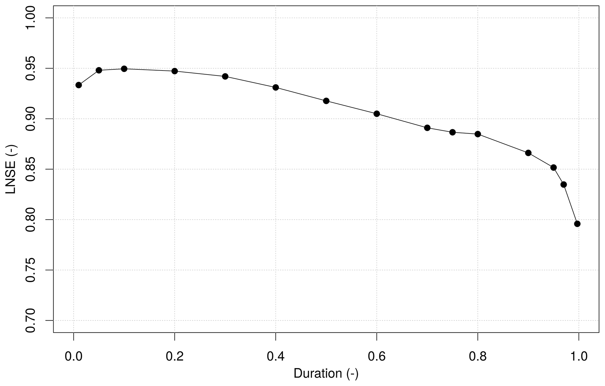
Figure 5Cross-validation (LOOCV) of predicted dimensional FDCs. LNSE values are reported as a function of duration.
3.3 Assessment of prediction uncertainty
The above-mentioned outcomes refer to aggregated measures of reliability. Given the wide extension of the study area, it becomes apparent that the TNDTK predictions of the streamflow regime are associated with different degrees of reliability, which varies significantly over the study area. Therefore, we develop for the entire study region (i.e. the European continent) a measure of uncertainty to be attached to FDC predictions. This measure should guide practitioners and users of interpolated FDCs, providing them with an operational tool for judging the suitability of the predicted FDCs for the water problem at hand. In order to assess prediction uncertainty (i.e. an estimate of the interpolation error), one can exploit the prediction variance, which is an output of top-kriging, as with any kriging-based interpolation procedure (Castellarin et al., 2018). This statistic is a combination of model uncertainty and configuration of observation locations: lower kriging variances are expected for large prediction catchments surrounded by several stream gauges, whereas higher variances are expected for prediction nodes located in data-scarce sub-areas and in upstream catchments. Figure 6 reports the moving average of standardized prediction variances (i.e. standardization with the maximum value, y axis) as a function of LNSE values (x axis) for a subset of 150 catchments. Note that, for the 2484 high-quality stream gauges, only 2102 LNSE values are available: the presence of measured or estimated percentiles of daily flows equal to zero makes the evaluation of LNSE impossible for 382 stream gauges.
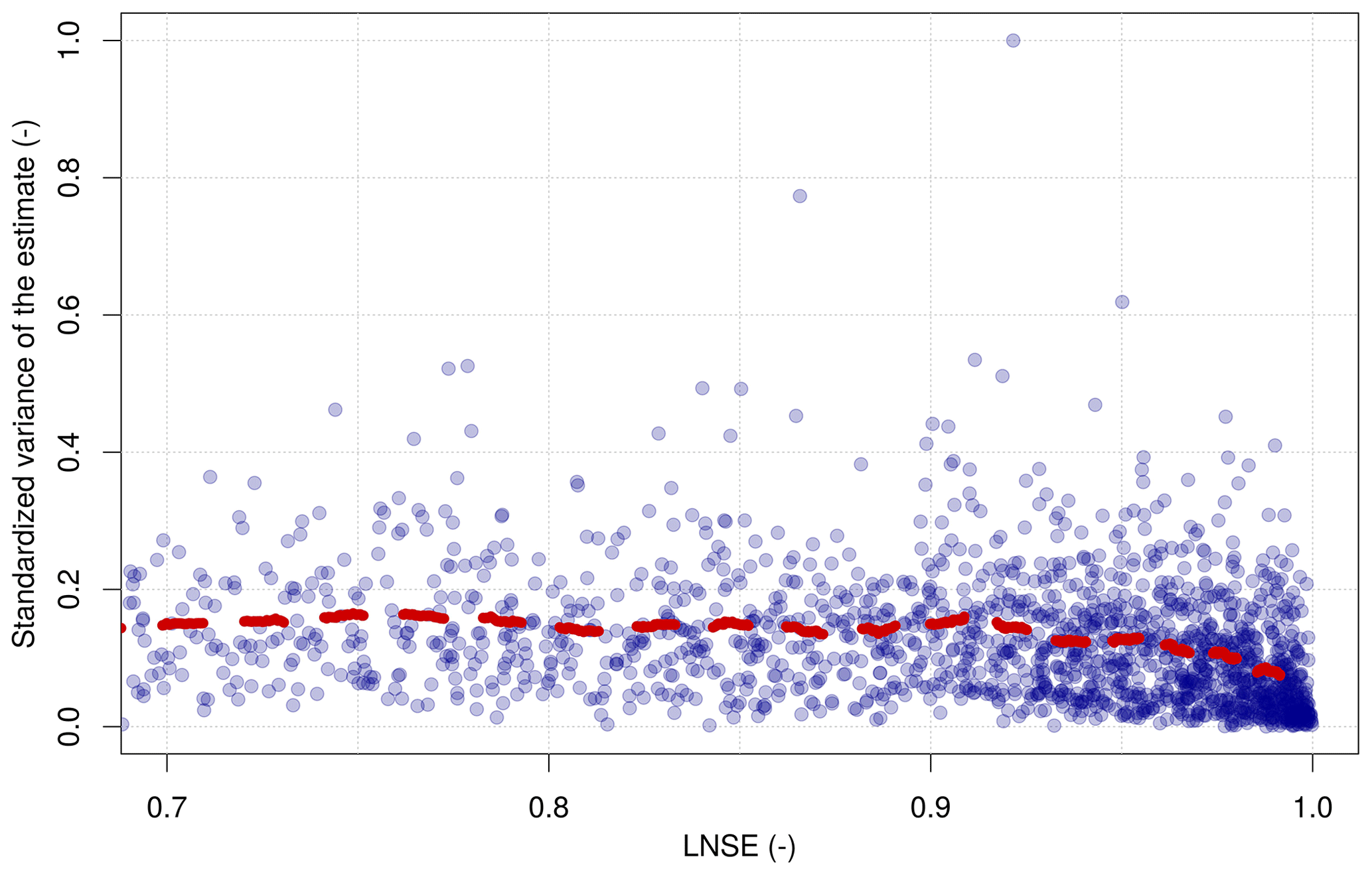
Figure 6Standardized prediction variance of TNDTK as a function of LNSE. LNSE values smaller than 0.7 are omitted here. The red dashed line represents the moving average computed with a moving window of 150 catchments. Note that, for the 2484 high-quality stream gauges, only 2102 LNSE values are available.
As observed in Castellarin et al. (2018) for the Danube region, Fig. 6 confirms for the European continent that higher LNSE values are associated with lower prediction variances. This information is useful for the application of TNDTK to ungauged basins since the average density of prediction nodes for the European region (i.e. approximately prediction points per square kilometre) is significantly higher than the stream-gauging network density (i.e. approximately gauges per square kilometre for high-quality data).
Table 1Description of fields of the produced GIS layer reporting predicted FDCs for the entire European continent. Note that only the 2484 catchments with high-quality data are considered to be gauged and are used for predicting FDCs in ungauged locations.
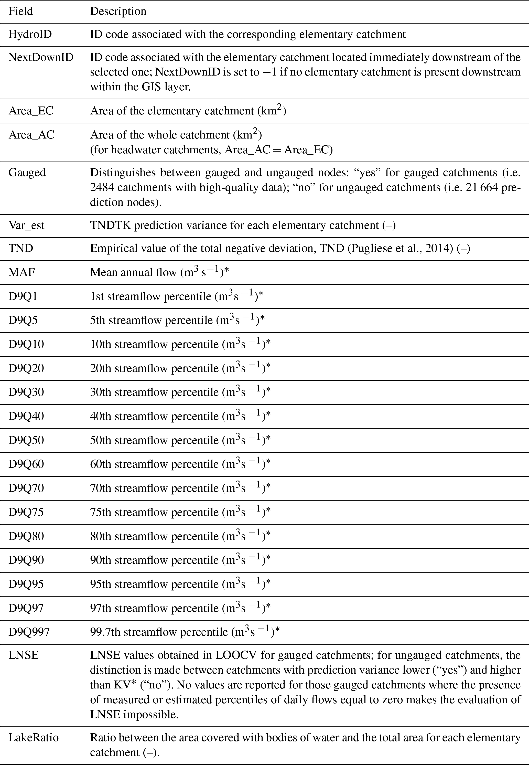
* If the “Gauged” field is equal to “yes”, then the marked values are empirical, while they are predicted otherwise.
3.4 Qualitative indicator of prediction accuracy
Furthermore, aiming at providing a qualitative assessment of the accuracy of predicted FDCs, we refer the reader to Fig. 6. First of all, we standardize prediction variances with the maximum value (0.28) among gauged and ungauged catchments, and then we compute a threshold value KV* (where KV stands for kriging variance) as the value below which the number of gauged catchments with LNSE <0.8 is equal to 5 % of the total number of gauged stations. Then ungauged catchments with standardized prediction variances lower and higher than KV* are labelled with “yes” and “no”, respectively. For gauged catchments LNSE values obtained in LOOCV are attached.
The data produced in this study are freely available at the PANGAEA open-access library (Data Publisher for Earth & Environmental Science) at https://doi.org/10.1594/PANGAEA.938975 (Persiano et al., 2021b). The dataset consists of a GIS vector layer of the contours of 24 148 elementary catchments contained within the white area reported in Fig. 3. The elementary catchments include both the 2484 high-quality gauged catchments and the 21 664 prediction nodes for which FDCs are estimated. Table 1 reports a summary of the information associated with each catchment, including the predicted FDCs' percentiles and the measures of uncertainty and accuracy described above. The file is stored using the ESRI shapefile format in the ETRS89 (European Terrestrial Reference System 1989) LAEA (Lambert azimuthal equal area) datum and geographic coordinate system.
All the activities regarding data preparation, analysis and representation of results have been produced by using free and open-source software (i.e. Quantum GIS Geographic Information System – Open Source Geospatial Foundation Project, http://qgis.osgeo.org (QGIS Development Team, 2022), and the R Project for Statistical Computing, https://www.R-project.org/, R Core Team, 2022). A repository containing an application example for extracting POR FDCs from daily streamflow series observed at gauged sites and computing FDCs at ungauged target sites by means of total negative deviation top-kriging (TNDTK; Pugliese et al., 2014, 2016) is available at the following link: https://doi.org/10.5281/zenodo.4751160 (Persiano, 2021). Together with the R codes and example data, the above-mentioned link also includes an RPubs link to an R-Markdown notebook containing step-by-step comments on the main R code. The specific R codes used for data preparation and analysis presented in this paper are made available by the authors upon request.
The present study describes an original spatial dataset providing a continuous representation of the streamflow regime for 24 148 elementary river catchments across Europe. For each elementary catchment, the boundaries are provided together with the value of the corresponding drainage area (for both the elementary and whole catchments), mean annual flow (i.e. long-term average daily discharge) and a set of 15 streamflow quantiles for durations from 1 to 99.7 % (i.e. flow-duration curves, FDCs). The streamflow indices (i.e. mean annual flood and FDCs) were estimated by means of the TNDTK geostatistical procedure (i.e. total negative deviation top-kriging) that, relying on a relatively small amount (compared to macro-scale models) of input data (i.e. observed streamflow series and catchment size and mutual position), allows one to predict the natural streamflow regime (i.e. FDCs) over large areas. In the present study, TNDTK relied on the empirical observations available for about 3000 discharge measurement stations included in the dataset itself.
Consistent with what was observed by Castellarin et al. (2018) for the Danube region, the adopted procedure provides an overall good accuracy for the entire study area (i.e. the European continent), with a reliability which can vary significantly in space, depending mainly on stream-gauging network density. For this reason, for each catchment we provide indicators of the accuracy and reliability of the performed large-scale geostatistical prediction, i.e. a measure of the prediction performance for gauged elementary catchments and a measure of uncertainty (i.e. estimate of the interpolation error, associated with kriging variance) for the streamflow indices estimated at ungauged catchments. These measures should provide practitioners and users with an operational tool for judging the suitability of the predicted FDCs for the water problem at hand.
Overall, the dataset made available herein is expected to be useful for the evaluation of water resource availability at ungauged locations and as a benchmark for the development of hydrological macro-scale models, whose local performances are highly variable. For instance, based on FDCs, Pugliese et al. (2018) show that TNDTK can be a useful tool for enhancing results from macro-scale models along the stream network of a given region, with significant advantages even for very low stream-gauging network densities. Such an enhancement procedure (Pugliese et al., 2018) does not explicitly account for the uncertainty associated with the predicted FDC, yet the prediction variance (included in our published dataset) returned by TNDTK can be used as a guide for benchmarking and enhancing macro-scale models.
SP wrote the paper and, together with AP, developed the R scripts, performed the analyses and produced the figures. AA and JOS provided support regarding the source data used for the analysis and the methodologies. AC and AP contributed to the development of the paper idea and supported the writing process of the manuscript.
The contact author has declared that none of the authors has any competing interests.
Publisher's note: Copernicus Publications remains neutral with regard to jurisdictional claims in published maps and institutional affiliations.
The source data used for this analysis were compiled by the Joint Research Centre of the European Commission (DG-JRC) from the archives of the International Commission for the Protection of the Danube River (ICPDR) and the Global Runoff Data Centre (GRDC). Both institutions are thanked for providing the data.
This paper was edited by Lukas Gudmundsson and reviewed by two anonymous referees.
Archfield, S. A., Pugliese, A., Castellarin, A., Skøien, J. O., and Kiang, J. E.: Topological and canonical kriging for design flood prediction in ungauged catchments: an improvement over a traditional regional regression approach?, Hydrol. Earth Syst. Sci., 17, 1575–1588, https://doi.org/10.5194/hess-17-1575-2013, 2013.
Castellarin, A.: Regional prediction of flow-duration curves using a three-dimensional kriging, J. Hydrol., 513, 179–191, https://doi.org/10.1016/j.jhydrol.2014.03.050, 2014.
Castellarin, A., Vogel, R., and Brath, A.: A stochastic index flow model of flow duration curves, Water Resour. Res., 40, W03104, https://doi.org/10.1029/2003WR002524, 2004.
Castellarin, A., Persiano, S., Pugliese, A., Aloe, A., Skøien, J. O., and Pistocchi, A.: Prediction of streamflow regimes over large geographical areas: interpolated flow–duration curves for the Danube region, Hydrolog. Sci. J., 63, 845–861, https://doi.org/10.1080/02626667.2018.1445855, 2018.
Castiglioni, S., Castellarin, A., Montanari, A., Skøien, J. O., Laaha, G., and Blöschl, G.: Smooth regional estimation of low-flow indices: physiographical space based interpolation and top-kriging, Hydrol. Earth Syst. Sci., 15, 715–727, https://doi.org/10.5194/hess-15-715-2011, 2011.
Ceola, S., Pugliese, A., Ventura, M., Galeati, G., Montanari, A., and Castellarin, A.: Hydro-power production and fish habitat suitability: Assessing impact and effectiveness of ecological flows at regional scale, Adv. Water Resour., 116, 29–39, https://doi.org/10.1016/j.advwatres.2018.04.002, 2018.
Collischonn, W., Allasia, D., Da Silva, B. C., and Tucci, C. E. M.: The MGB-IPH model for large-scale rainfall–runoff modelling, Hydrolog. Sci. J., 52, 878–895, https://doi.org/10.1623/hysj.52.5.878, 2007.
Cressie, N. A. C.: Statistics for spatial data, Rev. ed., Wiley, New York, 900 pp., https://doi.org/10.1002/9781119115151, 1993.
de Lavenne, A., Skøien, J. O., Cudennec, C., Curie, F., and Moatar, F.: Transferring measured discharge time series: Large-scale comparison of Top-kriging to geomorphology-based inverse modeling: transferring measured discharge time series, Water Resour. Res., 52, 5555–5576, https://doi.org/10.1002/2016WR018716, 2016.
de Paiva, R. C. D., Buarque, D. C., Collischonn, W., Bonnet, M.-P., Frappart, F., Calmant, S., and Bulhões Mendes, C. A.: Large-scale hydrologic and hydrodynamic modeling of the Amazon River basin: hydrologic and hydrodynamic modeling of the amazon river basin, Water Resour. Res., 49, 1226–1243, https://doi.org/10.1002/wrcr.20067, 2013.
Donnelly, C., Andersson, J. C. M., and Arheimer, B.: Using flow signatures and catchment similarities to evaluate the E-HYPE multi-basin model across Europe, Hydrolog. Sci. J., 61, 255–273, https://doi.org/10.1080/02626667.2015.1027710, 2016.
Falter, D., Dung, N. V., Vorogushyn, S., Schröter, K., Hundecha, Y., Kreibich, H., Apel, H., Theisselmann, F., and Merz, B.: Continuous, large-scale simulation model for flood risk assessments: proof-of-concept: Large-scale flood risk assessment model, J. Flood Risk Manag., 9, 3–21, https://doi.org/10.1111/jfr3.12105, 2016.
Farmer, W. H.: Ordinary kriging as a tool to estimate historical daily streamflow records, Hydrol. Earth Syst. Sci., 20, 2721–2735, https://doi.org/10.5194/hess-20-2721-2016, 2016.
Kroll, C. N., Croteau, K. E., and Vogel, R. M.: Hypothesis tests for hydrologic alteration, J. Hydrol., 530, 117–126, https://doi.org/10.1016/j.jhydrol.2015.09.057, 2015.
Laaha, G., Skøien, J. O., and Blöschl, G.: Spatial prediction on river networks: comparison of top-kriging with regional regression: spatial prediction on a river network: top-kriging versus regression, Hydrol. Process., 28, 315–324, https://doi.org/10.1002/hyp.9578, 2014.
Merz, R., Blöschl, G., and Humer, G.: National flood discharge mapping in Austria, Nat. Hazards, 46, 53–72, https://doi.org/10.1007/s11069-007-9181-7, 2008.
Pechlivanidis, I. G. and Arheimer, B.: Large-scale hydrological modelling by using modified PUB recommendations: the India-HYPE case, Hydrol. Earth Syst. Sci., 19, 4559–4579, https://doi.org/10.5194/hess-19-4559-2015, 2015.
Persiano, S.: SimonePersiano/TNDTK: Application example (v1.0.0), Zenodo [code], https://doi.org/10.5281/zenodo.4751160, 2021.
Persiano, S., Salinas, J. L., Stedinger, J. R., Farmer, W. H., Lun, D., Viglione, A., Blöschl, G., and Castellarin, A.: A comparison between generalized least squares regression and top-kriging for homogeneous cross-correlated flood regions, Hydrolog. Sci. J., 66, 565–579, https://doi.org/10.1080/02626667.2021.1879389, 2021a.
Persiano, S., Pugliese, A., Aloe, A., Skøien, J. O., Castellarin, A., and Pistocchi, A.: Streamflow data availability in Europe: a detailed dataset of interpolated flow-duration curves, PANGAEA [data set], https://doi.org/10.1594/PANGAEA.938975, 2021b.
Pugliese, A., Castellarin, A., and Brath, A.: Geostatistical prediction of flow–duration curves in an index-flow framework, Hydrol. Earth Syst. Sci., 18, 3801–3816, https://doi.org/10.5194/hess-18-3801-2014, 2014.
Pugliese, A., Farmer, W. H., Castellarin, A., Archfield, S. A., and Vogel, R. M.: Regional flow duration curves: Geostatistical techniques versus multivariate regression, Adv. Water Resour., 96, 11–22, https://doi.org/10.1016/j.advwatres.2016.06.008, 2016.
Pugliese, A., Persiano, S., Bagli, S., Mazzoli, P., Parajka, J., Arheimer, B., Capell, R., Montanari, A., Blöschl, G., and Castellarin, A.: A geostatistical data-assimilation technique for enhancing macro-scale rainfall–runoff simulations, Hydrol. Earth Syst. Sci., 22, 4633–4648, https://doi.org/10.5194/hess-22-4633-2018, 2018.
QGIS Development Team: QGIS Geographic Information System, Open Source Geospatial Foundation Project, http://qgis.osgeo.org (last access: 27 September 2022), 2022.
R Core Team: R: A language and environment for statistical computing, R Foundation for Statistical Computing, Vienna, Austria, https://www.R-project.org/ (last access: 27 September 2022), 2022.
Sampson, C. C., Smith, A. M., Bates, P. D., Neal, J. C., Alfieri, L., and Freer, J. E.: A high-resolution global flood hazard model: a high-resolution global flood hazard model, Water Resour. Res., 51, 7358–7381, https://doi.org/10.1002/2015WR016954, 2015.
Skøien, J. O. and Blöschl, G.: Spatiotemporal topological kriging of runoff time series: topological kriging of runoff time series, Water Resour. Res., 43, W09419, https://doi.org/10.1029/2006WR005760, 2007.
Skøien, J. O., Merz, R., and Blöschl, G.: Top-kriging - geostatistics on stream networks, Hydrol. Earth Syst. Sci., 10, 277–287, https://doi.org/10.5194/hess-10-277-2006, 2006.
Skøien, J. O., Blöschl, G., Laaha, G., Pebesma, E., Parajka, J., and Viglione, A.: rtop: An R package for interpolation of data with a variable spatial support, with an example from river networks, Comput. Geosci., 67, 180–190, https://doi.org/10.1016/j.cageo.2014.02.009, 2014.
Vogel, R. M. and Fennessey, N. M.: Flow-Duration Curves. I: New Interpretation and Confidence Intervals, J. Water Resour. Pl., 120, 485–504, https://doi.org/10.1061/(ASCE)0733-9496(1994)120:4(485), 1994.
Vogel, R. M. and Fennessey, N. M.: Flow duration curves II: a review of applications in water resources planning, J. Am. Water. Resour. Assoc., 31, 1029–1039, https://doi.org/10.1111/j.1752-1688.1995.tb03419.x, 1995.
Westerberg, I. K., Wagener, T., Coxon, G., McMillan, H. K., Castellarin, A., Montanari, A., and Freer, J.: Uncertainty in hydrological signatures for gauged and ungauged catchments: uncertainty in hydrological signatures, Water Resour. Res., 52, 1847–1865, https://doi.org/10.1002/2015WR017635, 2016.
Yaeger, M., Coopersmith, E., Ye, S., Cheng, L., Viglione, A., and Sivapalan, M.: Exploring the physical controls of regional patterns of flow duration curves – Part 4: A synthesis of empirical analysis, process modeling and catchment classification, Hydrol. Earth Syst. Sci., 16, 4483–4498, https://doi.org/10.5194/hess-16-4483-2012, 2012.