DeepOWT: a global offshore wind turbine data set derived with deep learning from Sentinel-1 data

Offshore wind energy is at the advent of a massive global expansion. To investigate the development of the offshore wind energy sector, optimal offshore wind farm locations, or the impact of offshore wind farm projects, a freely accessible spatiotemporal data set of offshore wind energy infrastructure is necessary. With free and direct access to such data, it is more likely that all stakeholders who operate in marine and coastal environments will become involved in the upcoming massive expansion of offshore wind farms. To that end, we introduce the DeepOWT (Deep-learning-derived Offshore Wind Turbines) data set (available at https://doi.org/10.5281/zenodo.5933967, Hoeser and Kuenzer, 2022b), which provides 9941 offshore wind energy infrastructure locations along with their deployment stages on a global scale. DeepOWT is based on freely accessible Earth observation data from the Sentinel-1 radar mission. The offshore wind energy infrastructure locations were derived by applying deep-learning-based object detection with two cascading convolutional neural networks (CNNs) to search the entire Sentinel-1 archive on a global scale. The two successive CNNs have previously been optimised solely on synthetic training examples to detect the offshore wind energy infrastructures in real-world imagery. With subsequent temporal analysis of the radar signal at the detected locations, the DeepOWT data set reports the deployment stages of each infrastructure with a quarterly frequency from July 2016 until June 2021. The spatiotemporal information is compiled in a ready-to-use geographic information system (GIS) format to make the usability of the data set as accessible as possible.

1 Introduction

Lately, the expansion of carbon-neutral energy is being strongly promoted (United Nations Framework Convention on Climate Change, Conference Of the Parties; COP26, 2021). Offshore wind energy is an efficient and reliable energy source and appears to be an important cornerstone for a renewable energy mix (Esteban et al., 2011). For example, the European Union (EU) plans to increase the installed offshore wind energy capacity from 12 GW in 2020 to 300 GW in 2050 with a view toward carbon-neutral energy production. Most of this expansion is planned in the North Sea basin (NSB), an already established hot spot for offshore wind energy production. Nevertheless, new sites in the Mediterranean Sea will be developed to achieve the stated goals (European Commission, 2020). The plans of the EU are exemplary for a global trend of expanding offshore wind energy projects. Offshore wind farms (OWFs) will be deployed to pre-established offshore wind energy production sites like the East China Sea (ECS). At the same time, the development of new sites for large OWFs, for example, in the Atlantic Ocean on the east coast of the United States, is ongoing (Rodrigues et al., 2015). Today, the offshore wind energy sector is starting a phase of massive expansion worldwide, affecting marine ecosystems (Drewitt and Langston, 2006; Wilson and Elliott, 2009; Bailey et al., 2014; Bergström et al., 2014; Slavik et al., 2019) as well as stakeholders of different socio-economic sectors that are active or interested in the same areas, like the fishing industry, shipping routes, military exclusion zones, cultural heritage, residents of coastal areas, or the recreational industry (Henderson et al., 2003; Wever et al., 2015; Gusatu et al., 2020; Gușatu et al., 2021; Virtanen et al., 2022). To foster the development of offshore wind energy and to provide all stakeholders with free access to data in order to ensure the most sustainable development possible, we introduce the DeepOWT (Deep-learning-derived Offshore Wind Turbines) data set, which reports offshore wind turbine (OWT) locations along with their deployment time series for 5 years, from 2016 until 2021, on a global scale.

The proposed DeepOWT data set has been derived from the Sentinel-1 radar archive by applying deep-learning-based object detection. The employed object detection models were completely trained on synthetic training examples generated by the novel Synthetic data generation in Earth Observation (SyntEO) approach (Hoeser and Kuenzer, 2022a). Thus, the methodological workflow enables the extraction of highly detailed information from extensive Earth observation archives. Hence, in addition to the offshore wind energy infrastructure locations, the temporal deployment process can be described at each detected location. This is of major interest for investigating the impact and optimisation measures during the deployment processes, which is an eventful and critical period in an OWT life cycle. Besides OWT locations, DeepOWT also provides locations of OWF substations and offshore wind energy infrastructure under construction in order to further increase the information depth and precision of a global OWT data set. In addition to this novel information, DeepOWT is openly accessible, comes with valuable ground truth data sets for spatial and temporal evaluation, and can easily be used in geographic information system (GIS) software due to its lightweight size (4.1 MB) and the established “.geojson” format.

2 Related research

The proposed study applies deep-learning-based image analysis to detect offshore wind energy infrastructures in Earth observation imagery. To provide an overview of the applied method and investigated application, Sect. 2.1 briefly introduces the application of convolutional neural networks (CNNs) in Earth observation. Furthermore, Sect. 2.2 gives an overview of the extraction of persistent marine infrastructures from Earth observation data with a specific focus on OWTs.

2.1 Deep-learning-based image analysis in Earth observation

During the “ImageNet Large Scale Visual Recognition Challenge” in 2012, Krizhevsky et al. (2012) proposed the “AlexNet” CNN, which won the aforementioned competition. The successful implementation of a deep learning model with many adjustable parameters by using an excessive amount of training data in combination with modern hardware like graphics processing units (GPUs) to optimise the model brought new attention to deep learning and neural networks from many research domains (Krizhevsky et al., 2017; LeCun et al., 2015). CNNs turned out to be particularly suitable for image analysis (e.g. for tasks such as image recognition, image segmentation, and object detection). These capabilities make CNNs the most widely used deep learning models in remote sensing (Zhu et al., 2017; Ma et al., 2019; Hoeser and Kuenzer, 2020).

In addition to optical and multispectral Earth observation data, deep learning models have also been increasingly used to analyse radar data from spaceborne Earth observation missions (Zhu et al., 2021). Baumhoer et al. (2019) and Dirscherl et al. (2021) demonstrated how U-Net-based CNNs can be used to extract the Antarctic coastline and supraglacial lakes from Sentinel-1 data respectively. Other examples of pixel-wise classifications or image segmentation tasks that exploit Sentinel-1 data with CNNs are the mapping of burned areas (Belenguer-Plomer et al., 2021), crop-type mapping (Cué La Rosa et al., 2018; Mullissa et al., 2018), or the classification of irrigated agricultural land (Bazzi et al., 2020). Closely related to the topic of persistent marine infrastructure in this paper is the application of ship detection with CNNs and Sentinel-1 data. A considerable number of studies have looked at the extraction of vessels from Sentinel-1 data by employing CNN-based object detection models; the reader is referred to Hoeser et al. (2020) for a comprehensive overview.

Multiple studies have demonstrated that CNNs can learn the spatial representation of target classes in Sentinel-1 images and that they can also consider the spatial context in these images to reduce false positives (Dirscherl et al., 2021; Kang et al., 2017; Hoeser and Kuenzer, 2022a). This property of CNNs is a particularly important argument for their use in extracting object classes from extensive, unfiltered satellite data archives, as demonstrated in this study.

2.2 Offshore wind turbine detection in Earth observation imagery

The detection of persistent offshore infrastructure in Earth observation data has been investigated by applying different approaches. A commonly used approach is the constant false alarm rate (CFAR), as used by Zhang et al. (2019) for marine infrastructure detection. Wong et al. (2019) combined the CFAR approach with a difference of Gaussians (DoG) preprocessing of remote sensing radar imagery to further increase the contrast between persistent marine infrastructure and the surrounding sea. Xu et al. (2020) applied order statistic filtering in combination with a derived set of thresholds to extract marine infrastructure from imagery provided by the Landsat and Sentinel-2 missions. Zhang et al. (2021) developed a handcrafted morphologic approach with manual thresholds to identify single OWTs in Sentinel-1 data. All of the aforementioned studies have the commonality that they strongly depend on the high contrast between offshore infrastructure and the surrounding open sea. In a preceding study to this data set, Hoeser and Kuenzer (2022a) proposed an adaptive, deep-learning-based object detection approach that takes multiscale spatial patterns of the target objects into account to distinguish further different types of offshore infrastructure in a single model.

Radar imagery, especially that provided by the Sentinel-1 mission, is an auspicious data source for studies related to the offshore wind energy sector. Besides the detection of persistent offshore infrastructures, the successful investigation of Sentinel-1 data for estimating wind energy potentials in near-coast and offshore areas (Majidi Nezhad et al., 2019) demonstrates the versatility of radar Earth observation data in the context of offshore wind energy production.

In 2022, there are three data sets that describe OWTs on a global scale, some of which are freely accessible. These are the 4C Offshore wind data set (4C Offshore, 2021), OWT locations in the Open Street Map (OSM) project, and the “global offshore wind turbine” (GOWT v1.3) data set by Zhang et al. (2021). The 4C Offshore wind data set collects information about offshore wind projects provided by OWF operators, project descriptions, and contracts. It provides an overview of OWF boundaries, single OWT locations and specifications, OWF substations, and export cables (4C Offshore, 2021). However, the private company 4C Offshore maintains the 4C Offshore wind data set and sells the information. Hence, the data set is only partly accessible to the public and can not be freely used in planning and research to its full extent.

The first open-source variant to mention is the OSM project, which provides OWT locations in its spatial database. As OSM data rely on the activity of the OSM community, the accuracy and completeness of the OWT locations vary from region to region. Hence, the data set accuracy is not spatially homogenous. Furthermore, there is only a limited temporal consistency in this data set. An entry made in OSM on a specific date does not necessarily correlate with its first appearance in the real world, especially when the temporal accuracy is narrowed down to weeks or months.

The GOWT v1.3 data set demonstrates the possibility for large-scale OWT detection by investigating Earth observation data. In its published version (version 1.3), it provides OWT locations from 2014 until 2019. Thus, an OWT location is reported as such when it first appears in a remote sensing image. In GOWT v1.3 there is no difference between OWTs under construction and those completed (Zhang et al., 2021). This class indifference leads to a temporarily shifted overestimation of the number of power-generating OWTs, as the construction phase is not provided separately. Furthermore, GOWT v1.3 does not separately classify OWF substations and has difficulties differentiating them from OWTs, which results in false positive detections of OWTs within OWF areas.

From these existing data sets and their limitations, the following characteristics have been derived for a global OWT data set:

• access to all OWT information, such as location and construction stage in a single file;

• a global extent with homogenous reliability;

• temporal consistency with respect to the date given in the data set for a single data point and its real-world appearance;

• differentiation between OWTs that are under construction and OWTs that are completed;

• differentiation between OWTs and OWF substations;

• the inclusion of the latest OWF projects independent of their size, location, and construction type.

The motivation of this study is to use a deep-learning-based object detection approach in order to derive a global offshore wind turbine data set with an information depth that is not yet freely available. To that end, we present the DeepOWT (Deep-learning-derived Offshore Wind Turbines) data set in this study. The main contributions are as follows:

• the presentation of a deep-learning-based object detection workflow with two cascading CNNs that detect offshore wind farms in the first stage and single offshore wind energy infrastructure facilities in the second stage;

• the application of the recently proposed SyntEO framework by Hoeser and Kuenzer (2022a) for using synthetic data to train the two supervised deep learning models;

• the introduction of the DeepOWT data set with offshore wind energy infrastructure locations on a global scale and quarterly deployment stages for each location from July 2016 until June 2021;

• the differentiation between offshore wind turbines, offshore wind energy substations, and offshore wind energy infrastructure under construction for each detected object in the DeepOWT data set;

• the generation of spatiotemporal ground truth data sets of offshore wind energy infrastructures for the two major wind energy production sites – the North Sea basin and the East China Sea;

• a comprehensive spatiotemporal evaluation of the automatically derived DeepOWT data set;

• free access to the DeepOWT data set and the ground truth data sets created.

3 Materials and methods

The upcoming sections introduce the investigated Sentinel-1 data (Sect. 3.1) and the workflow applied to obtain the proposed data (Sect. 3.2). The workflow describes how the training data for the deep learning approach are generated (Sect. 3.2.1) as well as how the CNNs are trained and used to extract offshore wind energy infrastructures (Sect. 3.2.2). The proceeding section (Sect. 3.2.3) explains how the deployment time series are derived for each extracted object. Finally, the evaluation process for the automatically derived results with hand-annotated benchmark data sets is described (Sect. 3.2.4).

3.1 Materials

The European Space Agency (ESA) Copernicus programme provides open access to continuously acquired Earth observation data (Aschbacher, 2017). As part of this programme, the spaceborne Sentinel-1 Synthetic Aperture Radar (SAR) mission covers mainland and coastal areas on a global scale with a 10 m pixel spacing. The active C-band radar system with a wavelength of 5.6 cm is independent of cloud coverage and is able to acquire images at both day and night (Torres et al., 2012). These specifications make the radar data of the Sentinel-1 mission an excellent source to monitor coastal environments and investigate OWTs on a global scale. All Sentinel-1 acquisitions with IW (interferometric wide), GRD (ground range detected), and VH (vertical sent–horizontal received) polarised specifications were chosen as underlying data in this study. Figure 1a shows how often a location on Earth is sensed by the two Sentinel-1 satellites (A and B) for the mentioned data product specification in the second quarter of the year 2021. The focus of the Copernicus programme becomes visible with a higher number of acquisitions over Europe. Here, the satellites acquire data on both ascending and descending orbits, with an inclination of 98.18^∘. This leads to an X-like pattern and a higher revisit rate compared with other parts of the Earth. In order to harmonise all quarterly acquisitions of the entire Earth to a single global mosaic with a pixel spacing of 10 m, all acquisitions were stacked and reduced to a single-band median composite (see Fig. 1b).

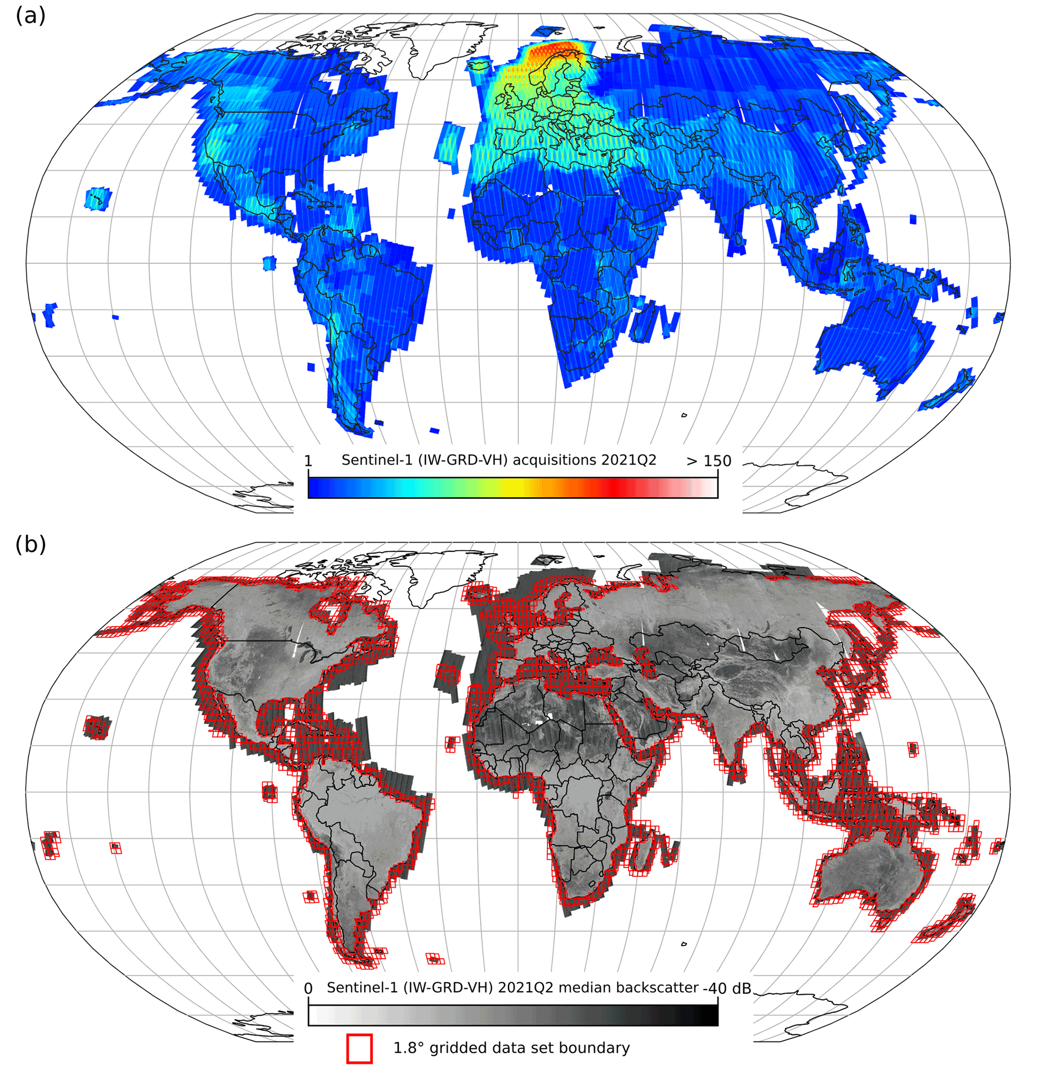
Figure 1 (a) The global distribution of the number of all available Sentinel-1 (IW–GRD–VH) acquisitions for the second quarter (Q2) of 2021. (b) The corresponding median backscatter amplitude and the data set boundary as a 1.8^∘ grid within a buffer of 200 km of the global coastline.

The extent of the study area is defined by a 200 km buffer of the OSM coastline towards the open sea. In order to systematically manage and process the data, a 1.8^∘ regular grid was generated for the entire Earth. All grid cells which intersect the 200 km buffer were selected. The final grid, pictured in Fig. 1b, defines the area where the DeepOWT data set was detected.

A global Sentinel-1 median composite was queried for the second quarter of 2021 (denoted as 2021Q2 hereafter). From this median composite, the global OWF and OWT locations were derived. The Google Earth Engine (GEE) (Gorelick et al., 2017) Python application programming interface (API) was used to query the Sentinel-1 data within each 1.8^∘ grid cell. The Sentinel-1 image collection in GEE provides the IW, GRD, and VH acquisitions with additional preprocessing for accurate orbit information, border and thermal noise removal, radiometric calibration, and terrain correction. The queried acquisitions within the 3-month period were reduced to a median composite with a pixel size of 10 m × 10 m and were then downloaded. To reduce the amount of data before downloading, the 16 bit floating-point number with a range of 0 to −40, which describes the Sentinel-1 backscatter signal in decibels, were rescaled to 0 to 255 and downloaded as 8 bit integers.

Quarterly subsets from 2016Q3 to 2021Q1 were generated the same way as the 2021Q2 global median composite to investigate temporal deployment dynamics. For these 19 quarterly subsets, the Sentinel-1 median composites were only created if a grid cell contained detected OWTs in 2021Q2. Thus, the underlying data for the DeepOWT data set are 20 quarterly sets from 2016Q3 to 2021Q2. The latest period in 2021Q2 holds a Sentinel-1 median composite of the entire global coastline. All other 19 sets only store Sentinel-1 median composites for OWF areas present in 2021Q2.

3.2 Methodology

Figure 2 shows an overview of the methodological workflow used to derive the OWT locations and their temporal deployment dynamics for the proposed data set. The core of the workflow is a cascade of two CNN object detectors: the first CNN detects the OWF boundaries, and the second CNN detects OWT locations on the 2021Q2 global median composite. In order to train both object detector CNNs, two synthetic training data sets were generated in a preceding step. This is the first application of the recently introduced SyntEO approach (Hoeser and Kuenzer, 2022a) embedded in a complete workflow to generate a global data set. After the OWT locations are detected in the 2021Q2 data, a time series of 19 quarterly periods is investigated to derive deployment dynamics for each OWT location from 2016Q3 until 2021Q1. In a final step, the OWT locations are refined from a bounding box to accurate point locations and are combined with the derived deployment time series. The combined spatiotemporal information is saved as a single file which comprises the DeepOWT data set.

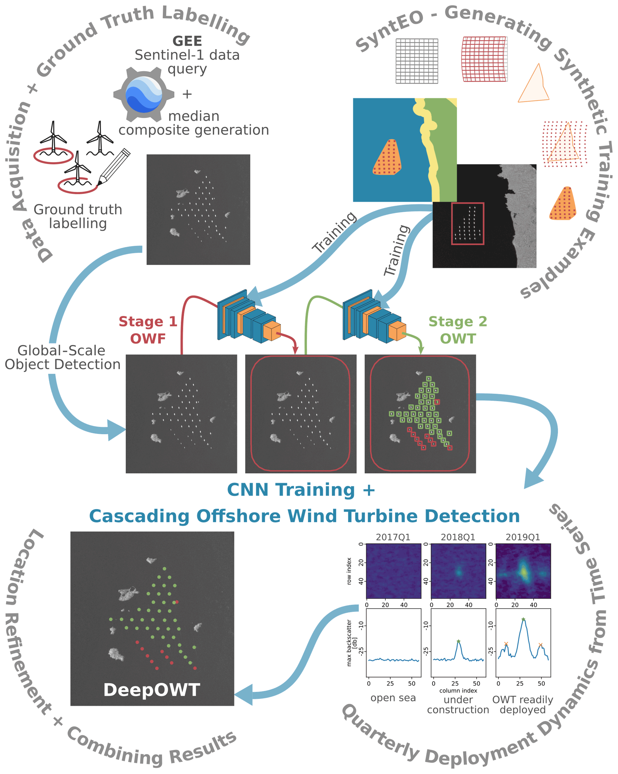
Figure 2 The methodological workflow used to generate the DeepOWT data set based on the Sentinel-1 archive. Two CNNs detect OWF and OWT locations, trained on synthetic examples. These spatial detections are used to define their temporal dynamics and an accurate location. Finally, DeepOWT combines these spatiotemporal results.

3.2.1 Synthetic training data set generation with SyntEO

In deep learning, layers of untrained weights are stacked to build deep neural networks. In order to adjust the weights in a neural network to succeed in a given task, a large data set with annotated examples is necessary for supervised training (LeCun et al., 2015). The annotation of such large training data sets by hand is time-consuming and, in the case of only a few real-world examples (e.g. OWFs), even impossible. In order to solve these problems, the SyntEO approach was introduced to automatically synthesise large annotated training data sets with a special focus on the needs of Earth observation data. In SyntEO, a domain expert formulates an ontology that describes entities in a remote sensing scene and their spatiotemporal interrelations. The SyntEO ontology is a complex description of nested entities that are related by using topological rules to describe their spatial dependencies. A synthetic image is generated upon the formulated ontology by composing spatially meaningful geometries of all entities to create an abstract scene composition. Hereinafter, sensor-specific texture is added to the geometries of the abstract scene composition to generate the final remote sensing image. Furthermore, annotations are simultaneously derived from the discrete geometries of the scene composition. Thus, large deep-learning-ready data sets can be created quickly and automatically. Figure 3 shows a visual summary of the SyntEO process for better intuition. For an in-depth explanation of the SyntEO framework and the underlying ontology concept for automatic data generation in Earth observation, we refer the reader to Hoeser and Kuenzer (2022a).

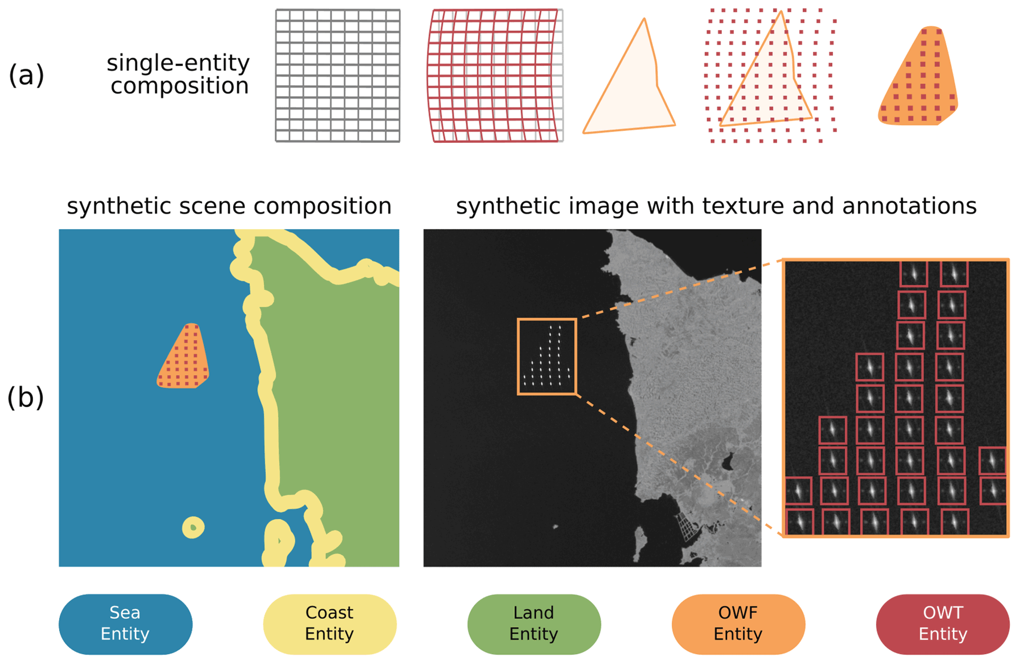
Figure 3 Simplified overview of a SyntEO workflow for automatic training example generation (Hoeser and Kuenzer, 2022a). Panel (a) visualises how the structure of a single OWF entity is generated. Panel (b) shows how multiple entities are composed to a scene composition. The final image is generated by adding texture to the composed scene. The bounding box annotations are derived from the scene composition.

For this study, the ontology drafted by Hoeser and Kuenzer (2022a) was extended to simultaneously generate training examples for OWF and OWT detection. In addition to the origin ontology, which only describes polygon-shaped OWFs, see Hoeser and Kuenzer (2022a), linear OWFs were introduced to increase the target object variance of the training examples. To further enrich the training data set, non-target classes like synthetically generated oil rigs and images that show the mainland were explicitly added with no annotations in order to provide negative training examples.

Furthermore, the ontology that has been formulated to generate training examples for OWF detection was reused for OWT detection. Most importantly, the size of the generated images and the annotation were changed. Instead of large-scale bounding box annotations for OWFs in synthetic images with a dimension of 2048 pixels × 2048 pixels, small-scale bounding box annotations for each OWT were derived from synthetic images with a dimension of 512 pixels × 512 pixels (see Fig. 3b). Thus, the CNN object detector, which detects OWTs and other offshore wind energy infrastructures, explicitly learns to focus on small-scale spatial features.

In order to include other targets besides readily deployed OWTs, the non-target class “oil rigs” in OWF detection was reused. In the second synthetic data set, variants of the generated oil rig signatures are employed to provide annotated examples for OWF substations and offshore wind energy infrastructure under construction. The mainland examples without annotation were kept to provide false positive training examples for OWT detection.

Two pools of training–annotation pairs with additional metadata were generated to compile two balanced synthetic training data sets: one training data set for OWF and one training data set for single offshore wind energy infrastructure detection. To enable the TensorFlow deep learning framework (Abadi et al., 2016), the selected image annotation pairs were parsed to the TFRecord binary format. Thus, the first training data set with 90 000 examples for OWF detection and the second training data set with 275 000 examples for OWT detection were created.

3.2.2 Global OWT object detection with CNNs

Deep learning has become an important driver for new insights and methodological developments in Earth system science (Zhu et al., 2017; Reichstein et al., 2019). Recent developments in CNNs have allowed for the detection of objects in large images by taking the spatial context into account (Hoeser and Kuenzer, 2020). For object detection, two-stage region-based CNN (R-CNN) models are the most commonly used architecture in Earth observation applications (Hoeser et al., 2020). To derive the DeepOWT data set, we used a cascade of two ResNet-50 (residual network with 50 convolutional layers) (He et al., 2016) faster R-CNN (Ren et al., 2015) models, where the first stage of the cascade detects OWF areas on a global scale, and the second stage detects single offshore wind energy infrastructure facilities within the previously detected OWF areas.

The first CNN for OWF detection ingests images with a dimension of 1024 pixels × 1024 pixels. This requires an on-the-fly downscaling of the training examples for OWF detection, which have a dimension of 2048×2048 pixels. For OWT detection in the second stage of the cascade, the training examples already have a dimension of 512 pixels × 512 pixels that matches the CNN architecture. Another difference in the model architectures for OWF and OWT detection is the adapted scale factors for the region proposal network (RPN), a submodule of the faster R-CNN object detector (Ren et al., 2015). In order to adjust the sensitivity for specific sizes of the target objects, the scale ratios were set to [0.25, 0.5, 1, 2, 3.5] for OWF and [0.25, 0.5] for OWT detection. The scale factors were calculated by applying the approach introduced by Hoeser and Kuenzer (2022a).

The training of the two CNNs was conducted on four parallel NVIDIA RTX 2080 Ti GPUs. The training schemes are the same for both architectures. A 0.95–0.05 training–validation split was prepared for both synthetic data sets. A single epoch without any data augmentation was used, which was possible due to the large size and variability of the synthetic data sets. The learning rate was scheduled to decrease smoothly by implementing the cosine decay method (Loshchilov and Hutter, 2016). After a warm-up phase, the base learning rate of 0.01 was reached and then reduced to 0 for all remaining training steps.

The two trained models were used in a cascading manner. The first stage detects OWF by applying a threshold of 0.5 on the prediction score. Thus, the first stage allows a higher false positive rate to include more OWF areas than necessary, but it avoids false omissions of OWF areas. The second stage detects single offshore wind energy infrastructure facilities within the potential OWF areas by applying a threshold of 0.75 to consider a valid prediction. With the second stage's results, the predictions of the first stage are refined. Potential OWF areas with a share of 90 % or more non-OWTs are belatedly dropped as false detections of stage one. This self-checking property of the cascade leads to a high detection rate with a low number of false omissions by simultaneously decreasing false detections. This property was highly suitable for scanning extensive Earth observation archives to find sparsely scattered target objects in large amounts of image data.

As all predictions are performed on overlapping input tiles, the same object can be detected multiple times. To summarise all predicted bounding boxes in one file, the pixel coordinates of the bounding boxes are translated to the World Geodetic System 1984 (WGS84) geographic coordinate system. Furthermore, the bounding boxes are sorted in descending order by their prediction score and indexed with $b=\mathrm{1},\mathrm{2},\mathrm{3}\mathrm{\dots }B$ in order to consolidate the bounding boxes that belong to the same object ℬ. This sorted list of bounding boxes ℬ_b was unified in a cascading manner if the next box of the list was completely within the unified box or if the boxes had an intersection over union (IoU) larger than τ_IoU=0.333 (see Eq. 1).

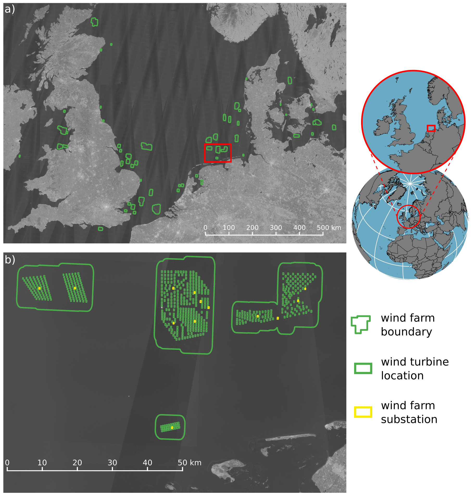
Figure 4 Detection results of the CNN cascade for the North Sea basin. Panel (a) shows the OWFs detected by stage 1, and panel (b) shows the OWT and OWF substations detected by stage 2 within the OWF boundaries of stage 1 in the German Bight.

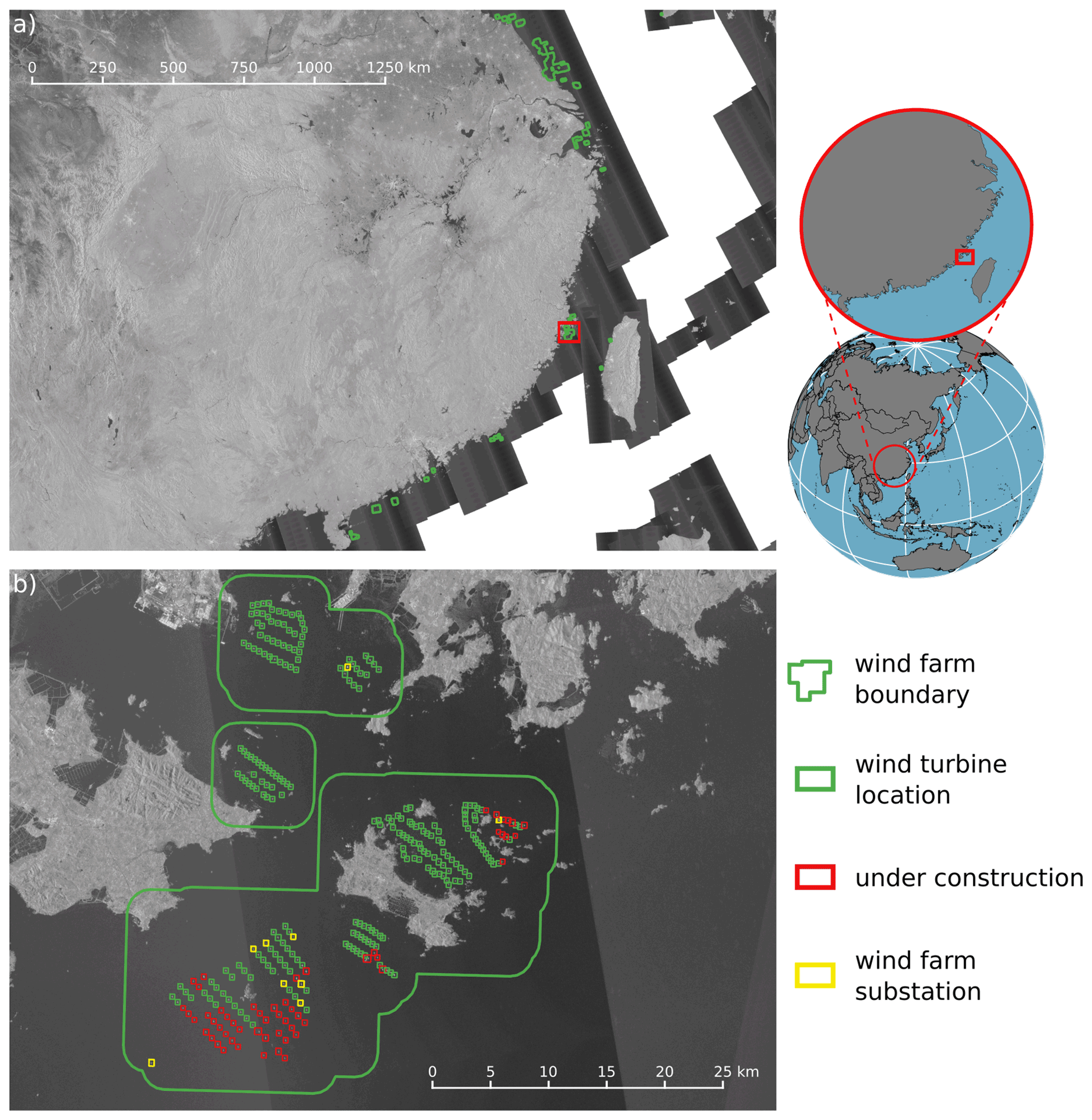
Figure 5 Detection results of the CNN cascade for the South and East China seas. Panel (a) shows the OWFs detected by stage 1, and panel (b) shows the OWTs, OWF substations, and such under construction detected by stage 2 within the OWF boundaries of stage 1 in the Taiwan Strait.

In order to calculate the exact area of each ℬ_b, the bounding box polygons were temporarily reprojected to their corresponding UTM (Universal Transverse Mercator) coordinate system depending on their UTM zone. The final unified polygons describe the OWF and OWT locations. Figures 4 and 5 show the detection results of the CNN cascade for northern Europe and south-eastern China respectively.

$$\begin{array}{}\text{(1)}& {\mathcal{B}}_{\mathrm{1}}:=\left\{\begin{array}{ll}{\mathcal{B}}_{\mathrm{1}}\cup {\mathcal{B}}_{b+\mathrm{1}}& \mathrm{if}{\mathcal{B}}_{b+\mathrm{1}}\subseteq {\mathcal{B}}_{\mathrm{1}},\\ {\mathcal{B}}_{\mathrm{1}}\cup {\mathcal{B}}_{b+\mathrm{1}}& \mathrm{if}\frac{{\mathcal{B}}_{\mathrm{1}}\cap {\mathcal{B}}_{b+\mathrm{1}}}{{\mathcal{B}}_{\mathrm{1}}\cup {\mathcal{B}}_{b+\mathrm{1}}}>{\mathit{\tau }}_{\mathrm{IoU}},\\ {\mathcal{B}}_{\mathrm{1}}& \mathrm{otherwise}.\end{array}\right.\end{array}$$

3.2.3 Time series analysis for deployment dynamics and location refinement

To describe the temporal dynamics of offshore wind energy infrastructure deployment, a backwards-looking time series analysis of the detected locations in 2021Q2 was performed. For each bounding box of an object location, a multitemporal stack of 19 quarterly Sentinel-1 median composites was analysed to determine if an image shows the open sea, an OWT or OWF substation under construction, or an OWT or OWF substation readily deployed. Swath profiles that describe each column's maximum value along the horizontal axes from each image in the multitemporal stack were generated. Figure 6 shows quarterly images and corresponding swath profiles for an OWT deployment time series. By applying two consecutive peak-finder algorithms with a high and low prominence (Virtanen et al., 2020) to the swath profile, the centre peak and adjacent peaks to the left and right of the centre peak were detected. In a subsequent analysis, which starts in 2021Q2 with the predicted class of the second stage CNN, the changes in the number of peaks, centre peak amplitude, and peak width are investigated to differentiate the deployment stages until 2016Q3.

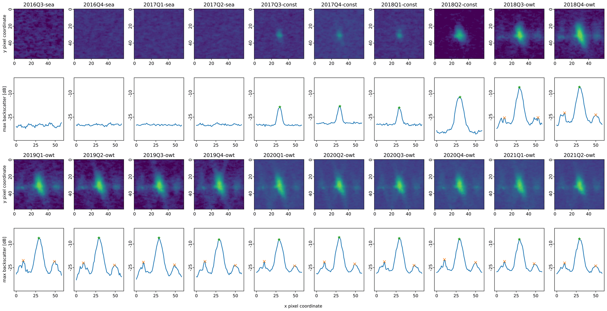
Figure 6 Deployment time series from 2016Q3 to 20201Q2 of an OWT. The first and third rows show quarterly Sentinel-1 median composites of the same detected bounding box over time. The second and fourth rows show the corresponding maximal swath profiles with detected peaks. The automatically derived construction stages are given for each image. The abbreviations used in the figure are as follows: sea – open sea/no turbine, const – under construction, and owt – offshore wind turbine.

To finally refine the bounding boxes of offshore wind energy infrastructure locations to point locations, all pixel values within each bounding box of the 2021Q2 period were analysed. As with the time series analysis, a maximum swath profile was created along the x axis, and the centre peak was searched for. With the derived x coordinate and amplitude of the centre peak, the column at the x location of the image patch within the bounding box was queried to find the corresponding y coordinate. By taking the geographic origin of the image patch into account, the WGS84 coordinate for this pixel was derived. Thus, the detected offshore wind energy infrastructure location is no longer described by a bounding box but by an accurate point location that is precisely at the centre amplitude maximum of the detected object. The final content for the derived data set is completed by merging spatial and temporal processing results.

3.2.4 Data set evaluation

In order to evaluate the DeepOWT data set, two ground truth data sets were generated. The test areas were the North Sea basin (NSB) and the East China Sea (ECS), pictured in Fig. 7. Their boundaries were aligned with the processing grid of this study. The two areas were chosen due to their importance for offshore wind energy generation; their differences concerning the underlying Sentinel-1 data; and the different interaction of OWFs with coastlines, coastal infrastructure, and islands. While the majority of OWFs in the NSB are located within a considerable distance of the coast, OWFs in the ECS are built in close proximity to small islands and other infrastructures like bridges and harbours (see Fig. 5). Furthermore, the NSB has a higher number of quarterly Sentinel-1 acquisitions in both orbit directions, whereas the ECS is mainly observed from a single orbit direction and, thus, has fewer acquisitions for the same time interval (see Fig. 1). This results in different characteristics of the global Sentinel-1 median composite in both areas. Together, the NSB and ECS represent various OWF types and how they appear in their natural environment; therefore, they are representational test sites.

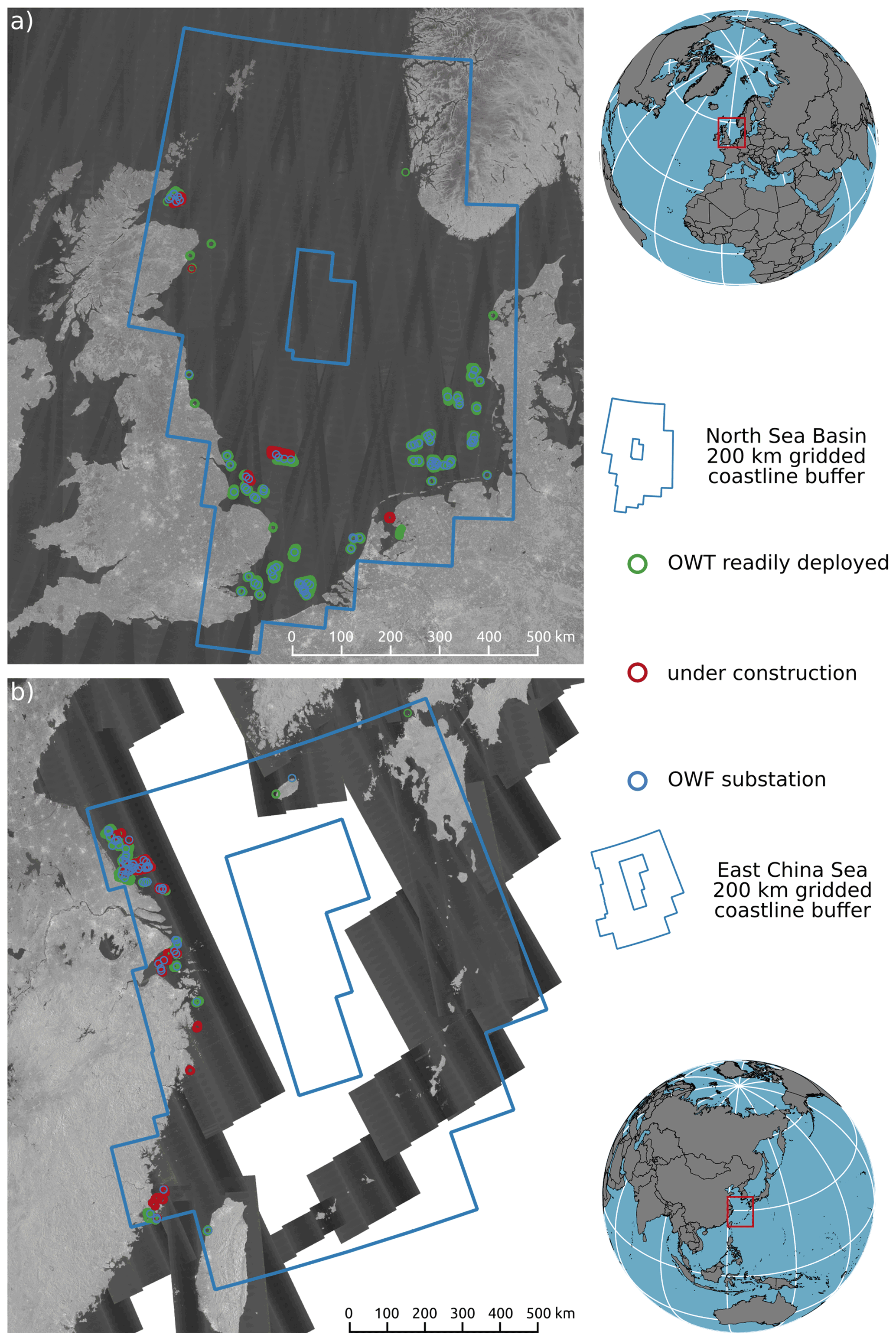
Figure 7 Overview of the ground truth sites' boundaries and the hand-labelled object locations and deployment stages for the second quarter of 2021. Panel (a) shows the North Sea basin (NSB), and panel (b) shows the East China Sea (ECS).

Two types of ground truth data sets were generated and included as separate files along with the proposed DeepOWT data set: the first type describes the locations of the target objects at a single point in time, and the second type describes quarterly time series of deployment dynamics.

Table 1 Overview of all ground truth data sets, their corresponding timestamp, and the number of objects in each class.

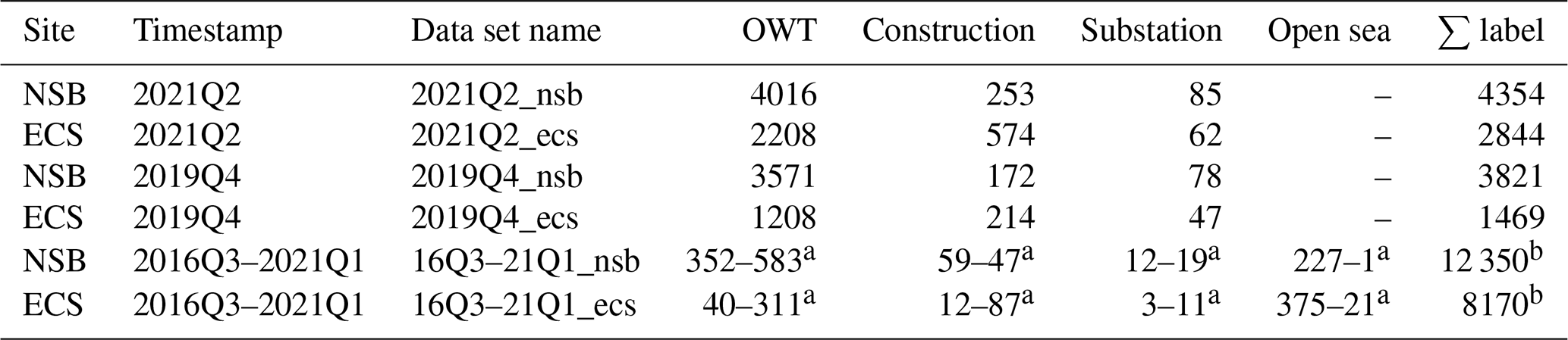
^a The numbers start in 2016Q3 and end in 20201Q1 of the ground truth time series. ^b The number of all hand-labelled classes for the entire ground truth time series with 19 intervals.

Two data sets of the first type were generated, one for 2021Q2 and one for 2019Q4. The 2019Q4 data set will later be used to compare the records of the DeepOWT data set to OSM and GOWT v1.3 records, as the latter ends in 2019. For both ground truth data sets, all locations of OWTs and OWF substations, both readily deployed or under construction, were annotated by hand for the entire NSB and ECS. Afterwards, the point locations were buffered with a radius of 100 m, which is the final area that defines a true positive location. To generate the temporal ground truth data sets, about 15 % of the 2021Q2 ground truth locations were selected for both the NSB and the ECS. For these selected locations, the entire quarterly time series from 2016Q3 until 2021Q2 was annotated by hand. An overview of the different ground truth data sets and their number of annotated target objects is provided in Table 1.

During manual ground truth data labelling, all locations and temporal intervals were visually examined and cross-checked against different data sources. Therefore, Sentinel-1 images were investigated in combination with additional RGB (red–green–blue) images from Sentinel-2 and Google Earth. Furthermore, public information concerning the deployment dynamics provided by official planning documents, OWF operators, and news portals was examined, mainly to validate the labels of the temporal ground truth data sets.

Following the manual generation of the ground truth data sets, we calculated evaluation metrics to assess the automatically derived DeepOWT data set. To provide consistent and comparable metrics that take the different numbers of objects for each test site into account, the metrics were calculated separately in the first step. A predicted object is considered a true positive (TP) when it is within the ground truth polygon (a 100 m radius around the object centre of a test label) and the predicted point and test polygon have the same class; otherwise, it is a false positive (FP). A wrongly omitted ground truth polygon is considered a false omission (FO). With TP, FP, and FO defined, precision Pr and recall Rc were calculated:

$$\begin{array}{}\text{(2)}& {\displaystyle }\mathrm{Pr}={\displaystyle \frac{\mathrm{TP}}{\mathrm{TP}+\mathrm{FP}}},\text{(3)}& {\displaystyle }\mathrm{Rc}={\displaystyle \frac{\mathrm{TP}}{\mathrm{TP}+\mathrm{FO}}}.\end{array}$$

The harmonic mean of Pr and Rc summarises both metrics as the F1 score:

$$\begin{array}{}\text{(4)}& \mathrm{F}\mathrm{1}=\mathrm{2}\times {\displaystyle \frac{\mathrm{Pr}\times \mathrm{Rc}}{\mathrm{Pr}+\mathrm{Rc}}}.\end{array}$$

Furthermore, all detections made by a CNN were sorted by their prediction scores in descending order and indexed with $c=\mathrm{1},\mathrm{2},\mathrm{\dots },C$. From this ordered list, an all-point interpolated precision–recall (PR) curve Pr_interp is generated:

$$\begin{array}{}\text{(5)}& {\mathrm{Pr}}_{\mathrm{interp}}=\underset{\stackrel{\mathrm{̃}}{\mathrm{Rc}}:\stackrel{\mathrm{̃}}{\mathrm{Rc}}\ge \mathrm{Rc}}{\max }{\mathrm{Pr}}_{\mathrm{interp}}\left(\stackrel{\mathrm{̃}}{\mathrm{Rc}}\right).\end{array}$$

Finally, the area under the all-point interpolated PR curve describes the average precision, AP, as follows (Padilla et al., 2021):

$$\begin{array}{}\text{(6)}& \mathrm{AP}=\sum _{c=\mathrm{1}}^C\left(\mathrm{Rc}\right(c)-\mathrm{Rc}(c-\mathrm{1}\left)\right)\times {\mathrm{Pr}}_{\mathrm{interp}}\left(\mathrm{Rc}\right(c\left)\right),\end{array}$$

where Rc(0)=0.

In order to report the overall metrics for all n sites or intervals of a time series, the separately calculated metrics were combined by macro-averaging:

$$\begin{array}{}\text{(7)}& {\displaystyle }{\mathrm{Pr}}_{\mathrm{avg}}={\displaystyle \frac{\mathrm{1}}{n}}\sum _{i=\mathrm{1}}^n{\mathrm{Pr}}_i;\text{(8)}& {\displaystyle }{\mathrm{Rc}}_{\mathrm{avg}}={\displaystyle \frac{\mathrm{1}}{n}}\sum _{i=\mathrm{1}}^n{\mathrm{Rc}}_i;\text{(9)}& {\displaystyle }\mathrm{F}{\mathrm{1}}_{\mathrm{avg}}={\displaystyle \frac{\mathrm{1}}{n}}\sum _{i=\mathrm{1}}^n\mathrm{F}{\mathrm{1}}_i.\end{array}$$

Thus, the macro F1_avg score is defined as the arithmetic mean over harmonic means following Opitz and Burst (2019).

4 Results

The derived DeepOWT data set contains 9941 offshore wind energy infrastructure locations on a global scale. Each detected location is associated with 20 quarterly deployment stages from July 2016 until June 2021, which provide information about the deployment process and the object class in order to further specify the offshore wind energy infrastructure type. The three potential classes are offshore wind turbines, offshore substations, and offshore wind energy infrastructure under construction. If no infrastructure object is present during a time interval, the class is set to open sea. Figure 8 provides an overview of all detected objects and their corresponding classes over the entire time series in the DeepOWT data set from July 2016 until June 2021.

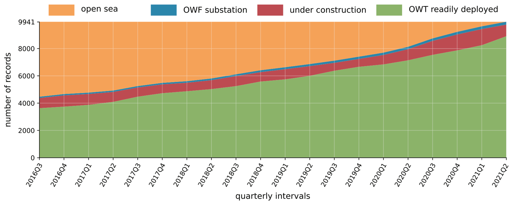
Figure 8 The temporal development of all 9941 objects and their corresponding class in the DeepOWT data set. The class and location in the interval 2021Q2 were derived using a CNN; in all other intervals, the class was derived by the swath profile analysis (see Fig. 6).

4.1 Evaluation results

Table 2 and Fig. 9 summarise the evaluation results of the objects detected by the CNN cascade in the latest interval (2021Q2). The evaluation results show that the performance is stable across both study sites. Thus, the CNN models trained on synthetic data can handle both test site characteristics equally well, despite the more challenging conditions in the ECS.

Table 2 Overview of all calculated metrics for the CNN cascade detections on the 2021Q2 global Sentinel-1 median composite for each class separately. The detections were evaluated with the 2021Q2_nsb (North Sea basin) and 2021Q2_ecs (East China Sea) ground truth data sets.

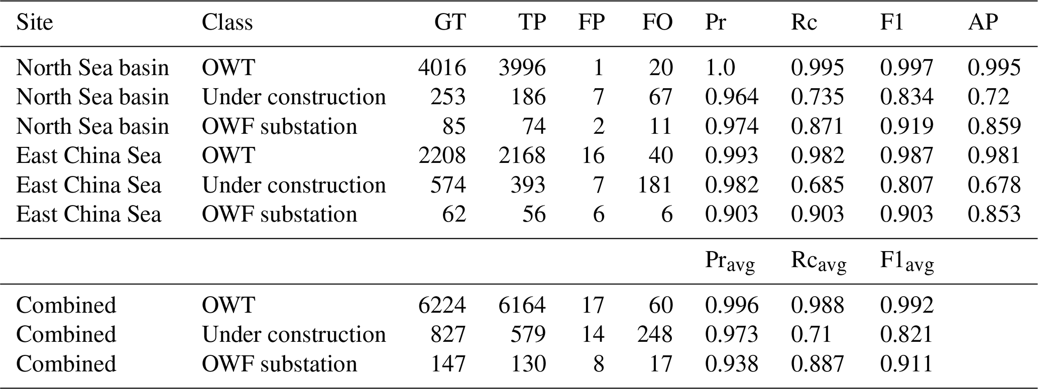
The abbreviations used in the table are as follows: GT – ground truth, TP – true positive, FP – false positive, FO – false omission, Pr – precision, Rc – recall, AP – average precision, and avg – average.

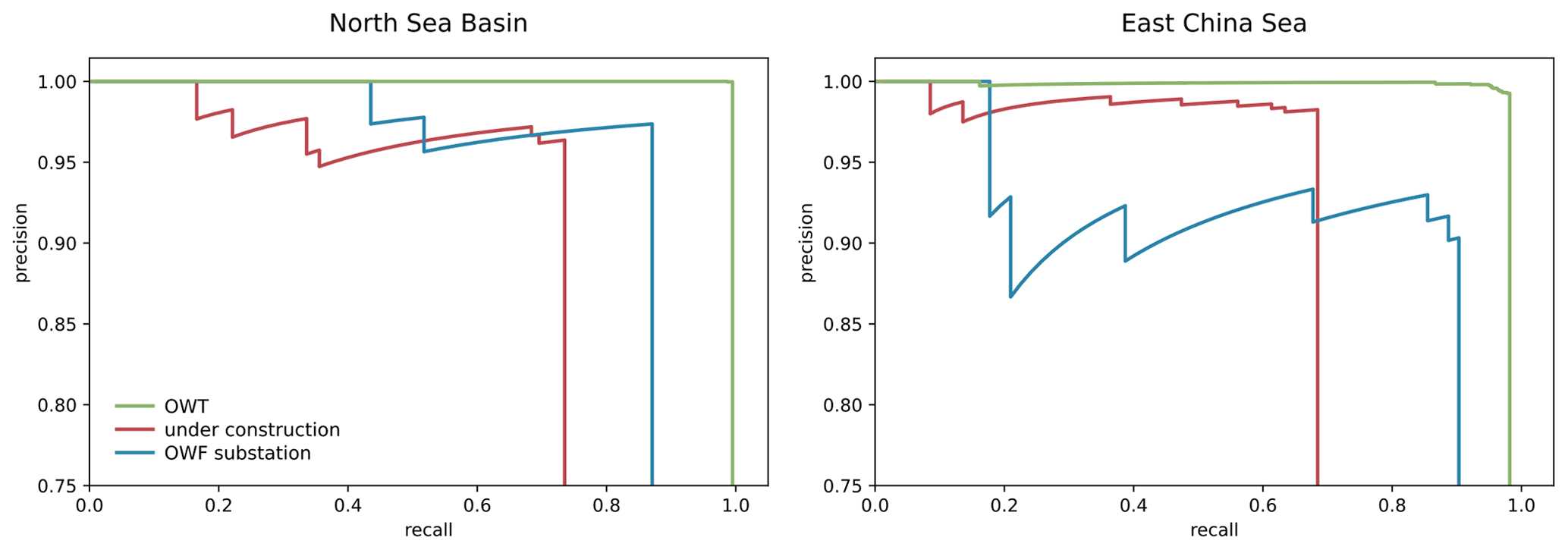
Figure 9 Precision–recall curves for the CNN cascade detections on the 2021Q2 global Sentinel-1 median composite for each respective class. The detections were evaluated with the 2021Q2_nsb (North Sea basin) and 2021Q2_ecs (East China Sea) ground truth data sets. The AP values from Table 2 are the corresponding areas under the interpolated precision–recall curves.

Figure 10 F1 scores for the quarterly intervals visualised as points, where the point size describes the number of ground truth labels. The panels on the right (boxplots) describe the F1 time series for each class and provide the temporal F1_avg over the entire time series. The data were evaluated on the 16Q3–21Q1_nsb (North Sea basin) and 16Q3–21Q1_ecs (East China Sea) ground truth data sets.

OWT detection is of the highest quality, with an F1_avg score of 99.2 %. Furthermore, the F1_avg score for OWF substations is 91.1 %. Offshore wind energy infrastructure under construction appears to be the most challenging class. This can be explained by the fact that the first real-world appearance of an OWT under construction can be restrained in median images when its onset is at the end of a quarter; thus, few Sentinel-1 acquisitions contribute to the quarterly median composite. Moreover, due to the unspecific spatial pattern of a single OWT under construction, they are falsely rejected because they are similar to small islands and other persistent marine infrastructure. The PR curve in Fig. 9 supports this interpretation: it clearly shows that it is always a true positive when an OWT under construction is recognised, resulting in high precision. However, the PR curve drops sharply at a high precision level around a recall level of 0.7. This indicates false omissions, which can also be seen in Table 2. However, the OWT under construction class still has an F1_avg score of 82 %.

Figure 10 shows the results of the time series evaluation. For each class and interval, the F1 scores were calculated. The boxplots on the right-hand side show their distribution and the F1_avg over the entire time series. The combined assessment reports the F1_avg in each period by averaging the corresponding results from the two ground truth sites. The results show that the time series analysis performs equally well on both sites, similar to the performance of the CNN cascade. OWTs have an F1_avg of 98.1 %, OWF substations have an F1_avg of 97.6 %, and offshore wind energy infrastructure under construction has an F1_avg of 81 %.

4.2 Data set comparison

As reported in Sect. 2, two openly accessible data sets exist that describe OWT locations: OWT records in the OSM database and the GOWT v1.3 data set (Zhang et al., 2021). As the GOWT v1.3 data set holds records until December 2019, all entries until 2019Q4 of the DeepOWT data set were chosen to perform the comparison. Likewise, for OSM records of OWTs, only those entries were queried that were registered by 31 December 2019. The evaluation metrics for all three data sets were calculated on the 2019Q4_nsb and 2019Q4_ecs ground truth data sets.

As OSM describes the locations of readily deployed OWTs, only the “owt” class from DeepOWT was assessed. The comparison in Fig. 11 shows the consistently better performance of DeepOWT compared with entries of the OSM database. It also becomes clear that the availability of OWT entries in the OSM database differs significantly between the two ground truth sites. In comparison, the records of the DeepOWT data set, which were derived from remote sensing data, show similar and consistently better performance metrics for both sites. This clearly shows the advantages of OWT detection based on remote sensing data on a global scale.

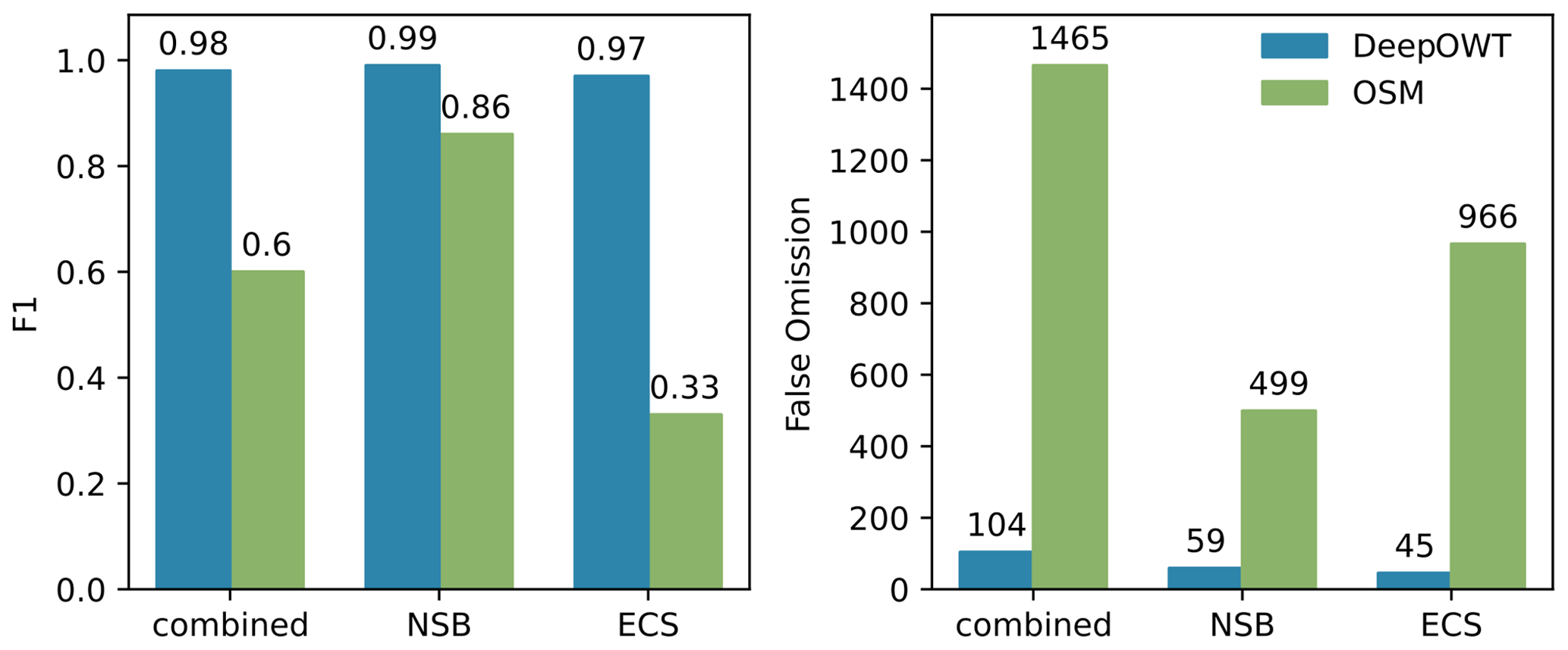
Figure 11 Comparison of the F1 score and false omissions from the OSM and DeepOWT data sets for readily deployed OWT locations in 2019Q4. The data sets were evaluated with the 2019Q4_nsb (North Sea basin) and 2019Q4_ecs (East China Sea) ground truth data sets.

GOWT v1.3 contains OWT locations, which are classified as such when the construction of a turbine foundation starts. However, it does not distinguish between OWTs under construction and those completed. Therefore, the “under construction” and “owt” classes of the DeepOWT data set were combined to compare the results with the GOWT v1.3 records. The comparison in Fig. 12 shows that both remote-sensing-based data sets perform consistently on both test sites. Nevertheless, this study's deep-learning-based DeepOWT data set performs better than GOWT v1.3, which has been derived by applying a handcrafted morphologic approach for OWT detection.

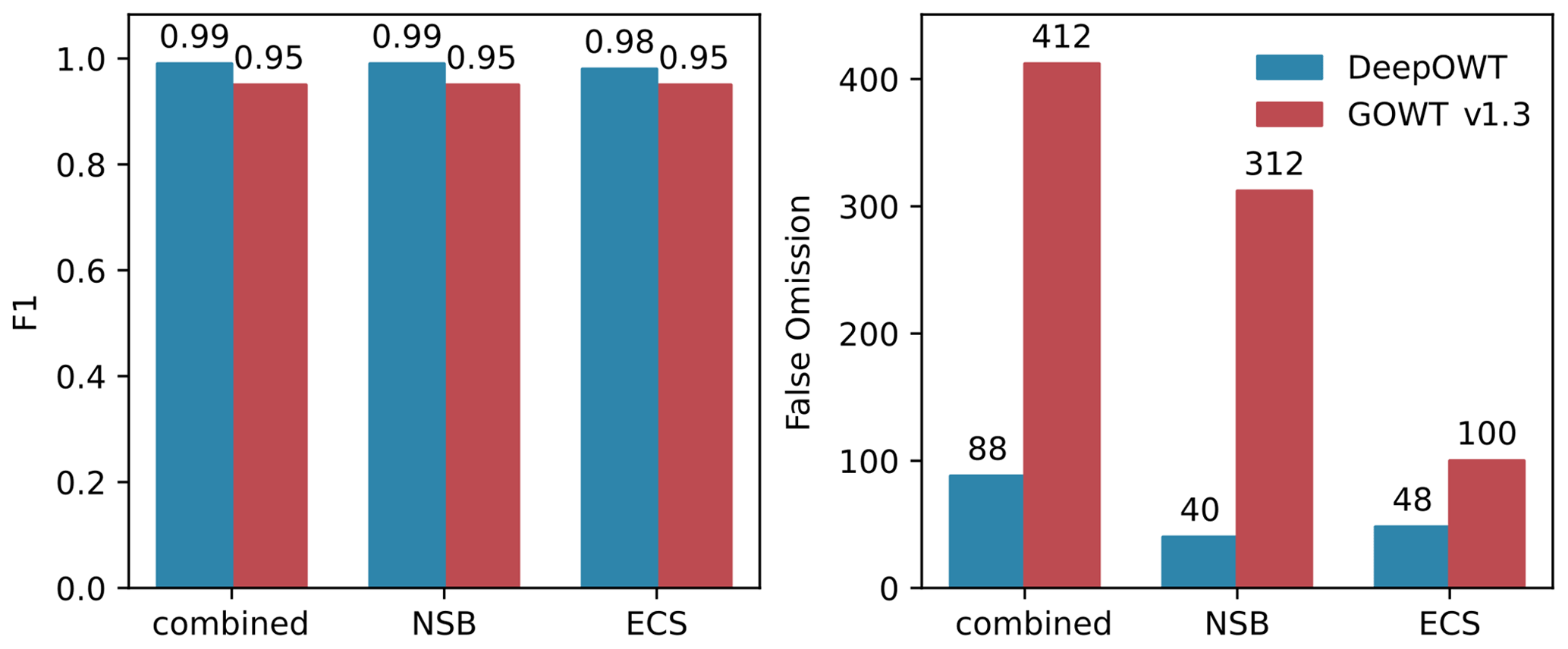
Figure 12 Comparison of the F1 score and false omissions from the GOWT v1.3 and DeepOWT data sets for readily deployed OWTs and OWTs under construction in 2019Q4. The data sets were evaluated with the 2019Q4_nsb (North Sea basin) and 2019Q4_ecs (East China Sea) ground truth data sets.

4.3 Technical description

The DeepOWT (Deep-learning-derived Offshore Wind Turbines) data set is introduced with version number 1.21.2: the first number is increased when significant changes are made to the methodology used to automatically detect the OWF and OWT objects or when additional content is appended to the data set, and the second and third numbers describe the year and quarter of the latest interval recorded in the data set. Thus, using this system, methodological and temporal information is incorporated into the data set name and versioning.

Table 3 Overview of the metadata of all files included in the DeepOWT data set.

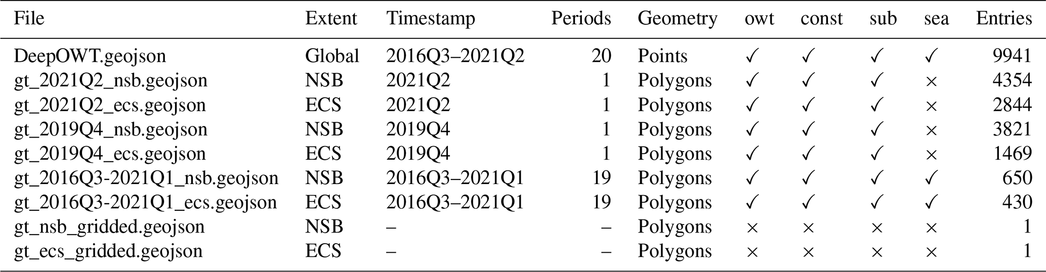
The abbreviations used in the table are as follows: owt – offshore wind turbine, const – under construction, sub – offshore wind farm substation, and sea – open sea.

The data set contains the automatically derived target location and the previously described hand-labelled ground truth data sets. Table 3 provides an overview of which data set file contains which information. DeepOWT 1.21.2 describes the deployment stages of OWT and OWF substations on a global scale from 2016Q3 to 2021Q2. Each entry holds the information of the deployment stage within 3 months of the respective quarter of a year. A total of 9737 OWTs were detected for the second quarter (Q2) of 2021. Of these, 8885 were readily deployed, and 852 were under construction. Additionally, 204 OWF substations were detected for the same period. The file size of DeepOWT is 4.1 MB.

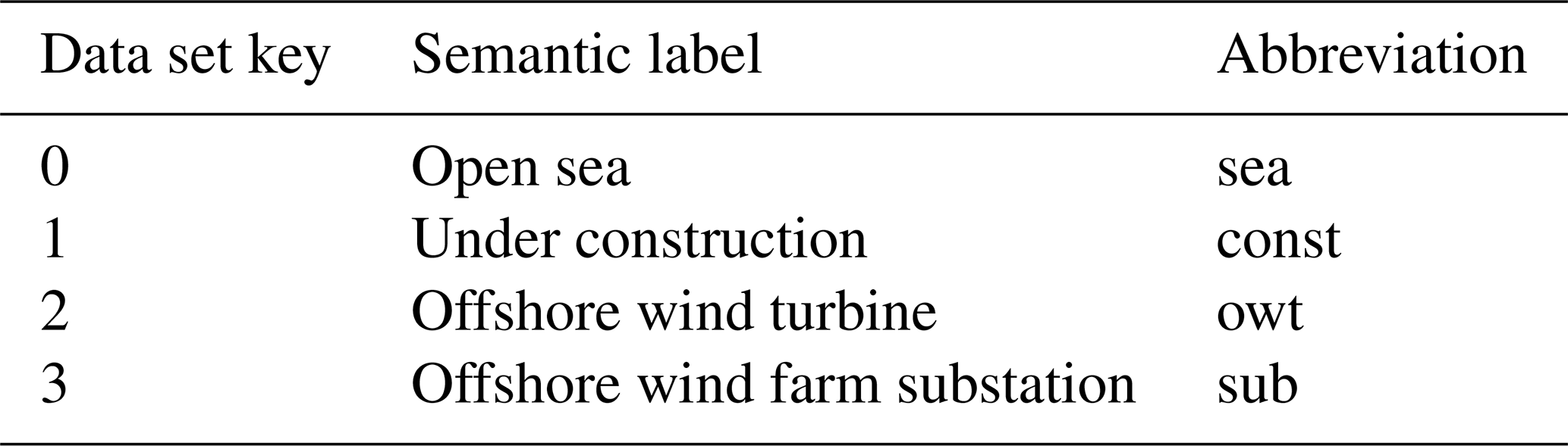
All automatically detected and hand-labelled objects are described as points or polygons using the WGS84 geographic coordinate system. The spatial geometries were checked topologically in order to identify duplicate entries, even if no topological errors were found during this inspection. The checked geometries were stored in .geojson files along with the temporal deployment information as a corresponding attribute table. The quarterly periods of the time series in the attribute table of a .geojson file are labelled using the following format: YyyyyQq, where yyyy is the year, and q is the quarter of a year. For each location and time series record, the object class or deployment stage is described as an integer between zero and three. Table 4 provides the mapping of the corresponding semantic labels.

Table 4 Mapping of the key in integer format (as used in the data set files) to semantic labels and their abbreviations.

4.4 Potential data set applications

Due to the increasing expansion of OWFs at existing and recently developed wind energy production sites, a holistic understanding and detailed insights into the expansion process are gaining importance (Fox et al., 2006; Gușatu et al., 2021; Johnson et al., 2022). The proposed DeepOWT data set enables all stakeholders involved to access OWT deployment time series globally. Therefore, the division into the pre-construction, intermediate, and post-construction phases of the deployment process is particularly important. OWT operators can use this information to develop optimisation measures for the necessary construction process with a specific focus on environmental conditions. Furthermore, single turbine locations on a global scale and under different conditions enable operators to investigate OWFs beyond their own facilities in order to optimise efficiency during the energy production phase and make better location decisions.

As OWFs often expand into areas that are already used as fishing grounds or shipping routes or into areas that are, to some extent, restricted areas like nature reserves or military exclusion zones, potential conflicts have to be recognised early and solved by integrated spatial planning towards multiuse concepts of marine space (Wever et al., 2015; Gusatu et al., 2020). DeepOWT supports the investigation and documentation of OWF projects and potential conflicts in order to apply the insights to upcoming projects in an early planning phase.

The ecological impacts of OWFs are varied and have to be differentiated using the spatiotemporal scale (Drewitt and Langston, 2006; Wilson and Elliott, 2009; Bailey et al., 2014; Bergström et al., 2014; Slavik et al., 2019). Thus the spatially contextualised deployment time series in DeepOWT are an important data source for investigations of how habitats and migration routes of marine wildlife are impacted. For policymakers, DeepOWT offers a quick overview of OWF expansion and the ability to compare trends on multiple scales in space and time (Rodrigues et al., 2015). Finally, DeepOWT can be used as a database to foster the exchange and transfer of knowledge between different stakeholders, which was found to be of high importance in offshore wind energy projects (Henderson et al., 2003; Fox et al., 2006; Wever et al., 2015; Gusatu et al., 2020).

From a technical perspective, DeepOWT offers a direct integration in analysis made with GIS software and spatial databases (Cavazzi and Dutton, 2016; Gusatu et al., 2020). The lightweight file size and structure of OWT locations, which summarise petabytes of underlying remote sensing images, enable fast processing, even on mobile devices. Thus, the DeepOWT data set can be used in computationally heavy GIS analysis as well as in field campaigns to enrich on-site mapping information.

5 Data availability

The DeepOWT data set is freely available from https://doi.org/10.5281/zenodo.5933967 (Hoeser and Kuenzer, 2022b). Additionally, the Coastal Explorer (https://coastalx.eoc.dlr.de/, last access: 3 August 2022), made with the UKIS Frontend library (Boeck et al., 2022), provides an interactive overview of the derived OWF boundaries and offshore wind energy infrastructure locations along with their temporal deployment dynamics.

6 Conclusions

This study introduced the DeepOWT (Deep-learning-derived Offshore Wind Turbines) data set, the first openly accessible data set that provides offshore wind turbine (OWT) locations along with their quarterly deployment stages on a global scale. DeepOWT is derived from the data provided by the Sentinel-1 spaceborne C-band radar mission. All available acquisitions along the global coastline between July 2016 and June 2021 were used to build quarterly median composites. The latest median composite from 2021 was investigated using deep-learning-based object detection. A cascade of two convolutional neural networks (CNNs) subsequently detects potential offshore wind farm (OWF) locations and single OWT and OWF substations within these areas. The two CNNs were trained entirely on synthetic training data generated using the novel approach for Synthetic data generation in Earth Observation, SyntEO (Hoeser and Kuenzer, 2022a). Based on the detections of the CNN cascade, a quarterly time series was derived that describes the deployment dynamics for every offshore wind energy infrastructure location between 2016 and 2021.

The data set covers 8885 OWTs, 852 platforms under construction, and 204 OWF substations for the latest period, the second quarter of 2021. The majority of OWTs are located in the North Sea basin and the East and South China seas. With equally good performance on the two ground truth data sets in the North Sea basin and East China Sea, the quality of the data set is consistent over time and space. DeepOWT securely describes large OWFs far off the coast as well as small OWFs in complex near-coastal environments. The DeepOWT data set contains nine .geojson files: one file with the predicted offshore wind energy infrastructure locations and deployment time series, and eight additional files that describe the ground truth data. With a file size of 4.1 MB, DeepOWT is easily portable and ready to use in GIS software.

DeepOWT contributes to a holistic understanding as well as detailed insights into the ongoing development of the offshore wind energy sector, which is at the beginning of a massive expansion phase on a global scale. Furthermore, DeepOWT proves the possibility of automatically detecting small-scale objects within large Earth observation archives of radar acquisitions without using auxiliary data by applying state-of-the-art deep learning methods. With the continuation of the Sentinel-1 mission secured, the future detection of OWT deployment time series on a global scale is possible.

Appendix A: Acronyms and abbreviations

AP	Average precision	GRD	Ground range detected
API	Application programming interface	GT	Ground truth
CFAR	Constant false alarm rate	IoU	Intersection over Union
CNN	Convolutional neural network	IW	Interferometric wide
COP26	United Nations Framework Convention on	NSB	North Sea basin
	Climate Change, Conference Of the Parties	OSM	Open Street Map
DeepOWT	Deep-learning-derived Offshore Wind Turbine data set	OWF	Offshore wind farm
DoG	Difference of Gaussians	OWT	Offshore wind turbine
EC	European Commission	Pr	Precision
ECS	East China Sea	PR	Precision–recall
ESA	European Space Agency	Rc	Recall
EU	European Union	ResNet-50	Residual network with 50 convolutional layers
F1	Harmonic mean of precision and recall	RGB	Red–green–blue
Faster R-CNN	Faster region-based convolutional neural network	RPN	Region proposal network
FO	False omission	SAR	Synthetic Aperture Radar
FP	False positive	SyntEO	Synthetic data generation for Earth Observation
GEE	Google Earth Engine	TP	True positive
GIS	Geographic information system	UTM	Universal Transverse Mercator
GOWT	Global offshore wind turbine data set by Zhang et al. (2021)	VH	Vertical sent–horizontal received
GPU	Graphics processing unit	WGS	World Geodetic System