the Creative Commons Attribution 4.0 License.
the Creative Commons Attribution 4.0 License.
 | 29 Aug 2022
A global map of local climate zones to support earth system modelling and urban-scale environmental science
Matthias Demuzere
Jonas Kittner
Alberto Martilli
Gerald Mills
Christian Moede
Iain D. Stewart
Jasper van Vliet
Benjamin Bechtel
There is a scientific consensus on the need for spatially detailed information on urban landscapes at a global scale. These data can support a range of environmental services, since cities are places of intense resource consumption and waste generation and of concentrated infrastructure and human settlement exposed to multiple hazards of natural and anthropogenic origin. In the face of climate change, urban data are also required to explore future urbanization pathways and urban design strategies in order to lock in long-term resilience and sustainability, protecting cities from future decisions that could undermine their adaptability and mitigation role. To serve this purpose, we present a 100 m-resolution global map of local climate zones (LCZs), a universal urban typology that can distinguish urban areas on a holistic basis, accounting for the typical combination of micro-scale land covers and associated physical properties. The global LCZ map, composed of 10 built and 7 natural land cover types, is generated by feeding an unprecedented number of labelled training areas and earth observation images into lightweight random forest models. Its quality is assessed using a bootstrap cross-validation alongside a thematic benchmark for 150 selected functional urban areas using independent global and open-source data on surface cover, surface imperviousness, building height, and anthropogenic heat. As each LCZ type is associated with generic numerical descriptions of key urban canopy parameters that regulate atmospheric responses to urbanization, the availability of this globally consistent and climate-relevant urban description is an important prerequisite for supporting model development and creating evidence-based climate-sensitive urban planning policies. This dataset can be downloaded from https://doi.org/10.5281/zenodo.6364594 (Demuzere et al., 2022a).
- Article
(15998 KB) - Full-text XML
- BibTeX
- EndNote


Cities are at the forefront of global climate change science owing to their emissions of greenhouse gases and their exposure to projected hazards, such as sea-level rise and climate warming (IPCC, 2022). As a result, they are the focus of mitigation and adaptation policies and, as they have governance structures in place, are an ideal scale to affect change. The crucial role that cities can play in this arena is recognized at the international level: the new United Nations Agenda and the 11th Sustainable Development Goal focus on urban resilience, climate, and environment sustainability of cities, two of the four challenges identified by the World Meteorological Organisation (WMO) World Weather Research Program are urban-related: high-impact weather, including impacts in cities, and urbanization, the Intergovernmental Panel on Climate Change Cities and Climate Change Scientific Committee identified six research priorities for science to have a stronger role in urban policy and practice, and advocacy groups like C40 (https://www.c40.org/cop26/, last access: 22 August 2022) play an increasingly important role in achieving national emission targets and enhancing resilience (Creutzig et al., 2016; Bai et al., 2018; Masson et al., 2020).
Cities are simultaneously drivers of regional and local climate changes. The conversion of earth's land surface into urban areas is one of the most irreversible human impacts on the global ecosystem (Grimm et al., 2008; Reba and Seto, 2020). In addition to the many modifications to the biosphere, hydrosphere, and lithosphere (Seto et al., 2012; D'Amour et al., 2017; Liu et al., 2019; van Vliet, 2019; Zhang et al., 2019; McDonough et al., 2020), urbanization affects energy demand (Creutzig et al., 2015; Güneralp et al., 2017), releases anthropogenic heat emissions and pollutants (Patella et al., 2018; Takane et al., 2019), and alters the urban climate (Oke et al., 2017). Current and future climate changes represent significant risks to urban populations and to the natural and physical infrastructure systems of cities (Costello et al., 2009; UN, 2019; Wang et al., 2021). In this context, the WMO has advocated the development of integrated urban services (IUS) – using observations (remote and on-site) and models – that addresses the panoply of hazards that cities face and the needs of service providers, including emergency services, public health bodies, energy produces, and urban designers and planners (Baklanov et al., 2018; Grimmond et al., 2020).
Despite their importance as a spatial nexus of climate drivers and of governance, cities are largely excluded from global climate science owing to their relatively small extent and our limited knowledge of their spatial structures. Global-scale climate models have only recently evolved to accommodate urban-scale landscapes, even though the urban parameters that are used by these models are limited in scope (Zhao et al., 2021). At regional and urban scales, model developments use far more detailed parameters that include descriptions of the net impacts of buildings in creating distinct urban canopy and boundary layers. While some theoretical challenges remain, it is now possible to simulate urban effects on climate between and above buildings at sub-urban scales (Barlow, 2014). Scientific advances will soon allow variable-resolution modelling that will incorporate the hierarchy of climate processes and impacts. However, the absence of suitable and universal global urban landscape data to inform these models represents a serious impediment to progress (Zhao et al., 2021; Hertwig et al., 2021). Hence, a comprehensive database is needed on cities globally that supports multi-scale modelling, provides a spatial framework for interpreting on-site and remote measurements, and allows the meaningful transfer of knowledge among and within cities (Rosenzweig et al., 2010; Hidalgo et al., 2018).
The critical data needed to support urban climate science include information on urban form and functions. Measures of form include e.g. building density, street widths, building heights, construction materials, and fraction of vegetated areas. These attributes largely influence the local climate and the “adaptation” capacity of a city (e.g. to ensure a comfortable thermal environment for its inhabitants). Urban functions describe the emissions of waste heat, materials, and gases into the overlying atmosphere. Appropriate measures would include the anthropogenic heat flux (AHF) and CO2 emissions. Form and function are correlated. For example, population density regulates energy consumption and therefore the potential to mitigate global warming by reducing the greenhouse gas emissions; variations in building layout and heights moderate surface roughness and contribute to the atmospheric dispersive conditions and thus the air quality (Martilli, 2014). Models are needed to assess the net benefits of climate-based interventions that may have unintended outcomes. For example, densely built and occupied cities (so-called compact 15 min cities) will reduce traffic, energy demand, and CO2 emissions and in some cases improve air quality (Stone et al., 2007; McDonough et al., 2020; Williams et al., 2010) but will enhance warming and heat stress by reducing vegetative cover and the sky view factor in the street canyons and increase the spatial density of the anthropogenic heat (Demuzere et al., 2014; Lai et al., 2019). Understanding how different urban forms interact with the atmosphere is key to redesigning cities, and, more importantly, planning future urbanization. It is therefore essential to have information that differentiates between urban forms that can be used by atmospheric models to simulate the future climatic conditions and different urban form scenarios. Our objective here is to generate these data to support model evolution and stimulate research on multi-scale climate projections to manage urban risks.
Acquiring urban data at a global scale is not a trivial exercise owing to the operational definition of “urban”, the scattered extents of cities globally, and their complex intra-urban geographies; for example, the Global Human Settlement Layer Urban Centres Database identifies over 13 000 settlements (Florczyk et al., 2019), while X. Li et al. (2020) generated over 60 000 global urban boundaries. At the global scale, there are several datasets that identify the extent of contiguous urban areas based on built-up or impervious surface cover (Zhou et al., 2015; Corbane et al., 2017; Esch et al., 2017; Marconcini et al., 2020; Gong et al., 2020; X. Zhang et al., 2020; Zhao et al., 2022) but none that provide intra-urban morphological details (green cover, built density, building heights, etc.) that are needed by scientists to generate the urban canopy parameters (UCPs) to run models and by urban policy-makers to make informed decisions based on analyses of risk. For many cities, relevant information may be gleaned from local sources that maintain municipal geographic databases (e.g. Biljecki et al., 2021), but these data vary in terms of their quality, consistency, and accessibility, which limits their wider applicability (Zhu et al., 2019). The 100 m-resolution global local climate zone (LCZ) map presented here addresses this need for more detailed intra-urban data. This product is the outcome of more than a decade of research on how best to acquire, evaluate, and deploy urban data in support of climate science (Stewart and Oke, 2012; Bechtel and Daneke, 2012; Ching et al., 2018).
The LCZ typology is currently the only universal classification that categorizes urban landscapes using a scheme that identifies readily recognizable neighbourhood types based on their form and function, which modify the surface energy and water budgets. Critically, each LCZ type is linked to meaningful UCP value ranges that can be used for physically based modelling (Stewart and Oke, 2012; Ching et al., 2019; Demuzere et al., 2020a). This goes beyond the urban mask and enables the assessment of the spatial impact of urban planning decisions that will alter UCPs and their climate outcomes. The LCZ scheme is distinguished from other LULC schemes by its focus on urban and rural landscape types, which can be described by any of the 17 classes in the scheme (Fig. 1). The scheme was originally designed to encourage climate change researchers to step away from their computers and get acquainted with the field sites that support their work in order to capture the character of the urban landscape responsible for the urban heat island (UHI) and to ensure consistent reporting of metadata about the sites used to measure the heat island effect (Stewart, 2018; Stewart and Mills, 2021). The World Urban Database and Access Portal Tools (WUDAPT) project has adopted the scheme in pursuit of its goal “to capture consistent information on cities worldwide that can support urban weather, climate, hydrology and air quality modelling” (Ching et al., 2018). The global LCZ product for the first time captures the intra-urban heterogeneity across the whole surface of the earth, capturing cities of all sizes. It complements the LCZ maps for individual cities created by the WUDAPT community, the LCZ Generator (https://lcz-generator.rub.de/, last access: 22 August 2022) (Demuzere et al., 2021), or those available via other sources (e.g. Taubenböck et al., 2020; Zhu et al., 2022). In addition, as each LCZ type is associated with generic numerical descriptions of key UCPs, the availability of this globally consistent and climate-relevant urban description is an important prerequisite for advancing our capacity to assess climate risks at urban scales and enabling the development of fit-for-purpose climate mitigation and adaptation strategies.
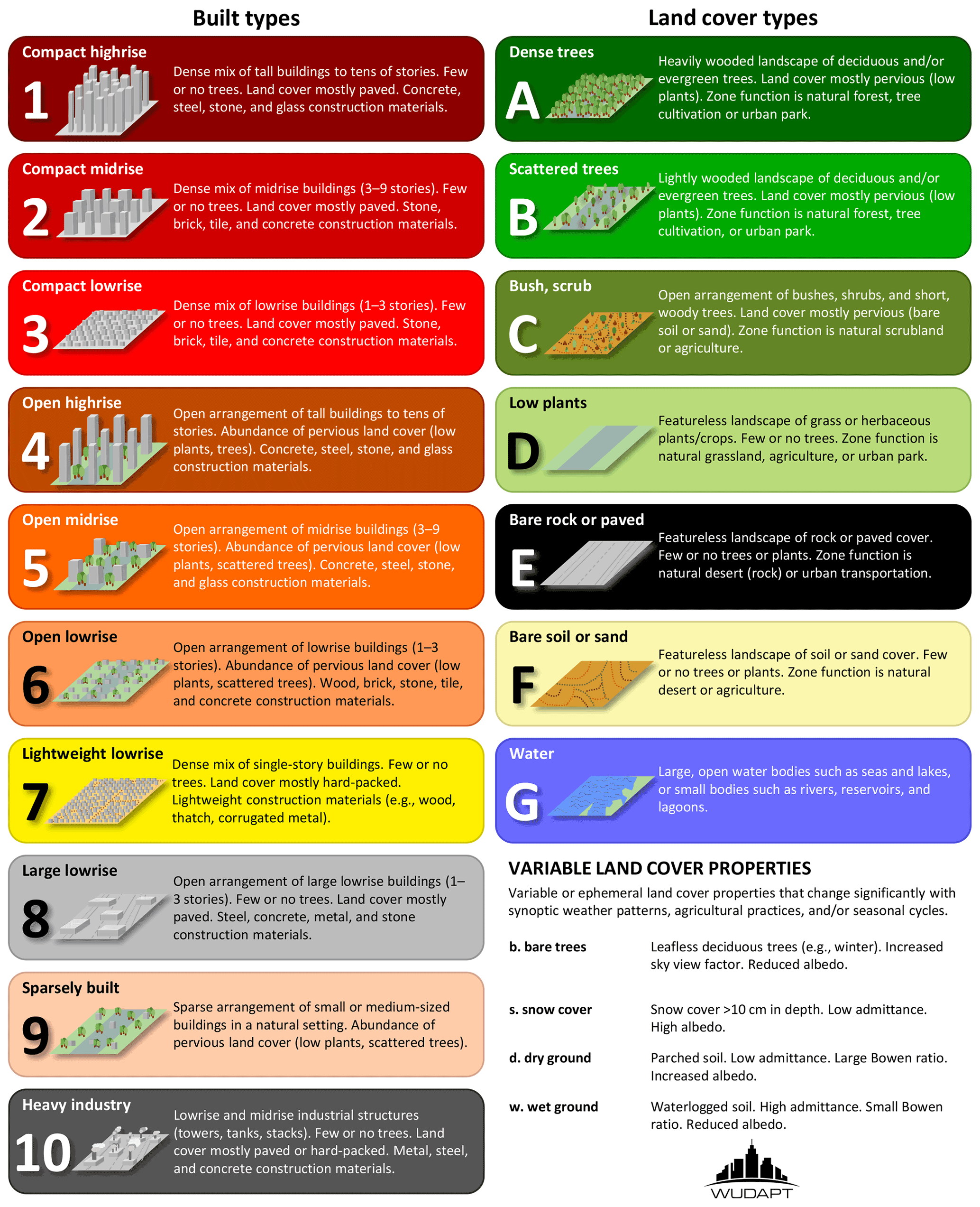
Figure 1Definitions of built (1–10) and land cover types (A–G) for the local climate zone scheme (Stewart and Oke, 2012; Demuzere et al., 2020a).
Whilst many LCZ mapping methodologies are currently available (see e.g. the review by Jiang et al., 2021), the methodology for the global LCZ map follows WUDAPT's default protocol that was launched by Bechtel et al. (2015) and sequentially improved by Demuzere et al. (2019b, a, 2020a), ultimately leading to the LCZ Generator (Demuzere et al., 2021), a web application that makes single-city LCZ mapping fast and easy. The procedure requires labelled training areas, earth observation input data, and a random forest classifier, discussed in depth in Sect. 2.1, 2.2 and 2.3 respectively. In addition, in line with previous continental-scale LCZ mapping efforts by Demuzere et al. (2019b, 2020a), the quality of the resulting LCZ map is assessed in two ways: (1) a traditional quality assessment using multiple accuracy metrics and (2) a thematic benchmark, by translating the LCZ map into its corresponding LCZ-based urban canopy parameters and comparing these against (semi-)independent global and open-source databases reflecting urban forms and functions (Sect. 2.4).
2.1 Training areas
Training areas (TAs) are LCZ-labelled polygons that represent typical examples of built or natural LCZs in a region of interest (ROI). By design, they are compiled in a crowd-sourced manner, either by urban experts (Bechtel et al., 2015) or alternative crowd-sourcing platforms such as MTurk (https://www.mturk.com, last access: 22 August 2022) (Demuzere et al., 2020a; Xu et al., 2021) using good-practice guidelines for digitizing TAs (see Appendix A and Demuzere et al., 2021). While the training area polygons and corresponding LCZ maps created by individuals are often of poor to moderate quality, the Human Influence Experiment (HUMINEX) (Bechtel et al., 2017; Verdonck et al., 2019a) demonstrated large accuracy improvements (up to 20 %) when multiple (poor- to moderate-quality) training datasets were used together to create a single LCZ map. In the current study, TAs are compiled from multiple sources. First, well-trained (inspired by HUMINEX findings) student assistants from the Ruhr-University Bochum produced TA sets for more than 100 global ROIs (labelled RUB). Second, archived TA (labelled ARC) sets were collected from previously published research and collaborations, including the samples hosted on the original WUDAPT portal (https://www.wudapt.org/the-wudapt-portal/, last access: 22 August 2022). Finally, the RUB and ARC TA sets are supplemented with the TA samples available from the LCZ Generator (Demuzere et al., 2021) (labelled GEN).
Before being used in the classification procedure, all TA sets are curated. First, all RUB and ARC training area sets are submitted to the LCZ Generator: in case of multiple entries for one submission, only the submission with the highest overall accuracy is retained. Second, only TA samples mapped to LCZs with an overall accuracy greater than 50 % are kept. Third, in case of duplicate regions across the different sources, the following priority is used: RUB > ARC > GEN. Fourth, only the original 17 LCZ classes are kept, thereby removing non-standardized classes available in some of the samples, such as LCZ W – “Wetlands” (Brousse et al., 2019, 2020b, a) and LCZ H – “Agricultural greenhouses” (Vandamme et al., 2019). Third, in order to maintain computational efficiency and to avoid redundancy and mixed spectral characteristics, the surface area of large polygons (>1.5 km2) is reduced, and too small or too complex TA polygons are removed (Demuzere et al., 2021). Finally, all pixels embedded within the ROIs are assigned to urban ecoregions (ERs), which are regional clusters based on climate, vegetation, and urban topology (Schneider et al., 2010). This is based on the finding of Demuzere et al. (2019b) that ERs can provide a basis for intelligent learning between cities and allow upscaling from individual cities to regional and global levels.
2.2 Earth observation input data
In addition to the TAs, earth observation (EO) input data are also required to feed into the LCZ-supervised random forest classifier (Breiman, 2001; Bechtel et al., 2015). The 33 global earth observation input features used by default in the LCZ Generator (see Table 2 in Demuzere et al., 2021) serve as a baseline. However, some EO input features are updated or added. The original 1 km global forest canopy height representative for 2005 (Simard et al., 2011) is replaced by the 30 m global forest canopy height dataset representative for 2019, developed by Potapov et al. (2021) through the integration of the Global Ecosystem Dynamics Investigation (GEDI) lidar instrument data (April–October 2019) and multi-temporal metrics derived from Landsat. Also, the ALOS digital surface model (DSM) data are updated to version 3.2, an improved version that reconsiders the format in the high-latitude area, auxiliary data, and processing method (Tadono et al., 2016). In addition, the Shuttle Radar Topography Mission (SRTM) digital elevation model (DEM) information is replaced by the MERIT DEM (Multi-Error-Removed Improved-Terrain Digital Elevation Model, Yamazaki et al., 2017), from which the slope and aspect are also added. Because of the changes in the DSM and DEM, the Canopy Height Model (CHM) (DSM–DEM) data are also updated. Building further upon the findings of Brousse et al. (2020a), Hay Chung et al. (2021), and Chen et al. (2021a), two more sets of input features are added, including (1) Gray Level Co-occurrence Matrix (GLCM) texture features (contrast, dissimilarity, inertia, sum average, and cluster shade) derived from the PALSAR (Phased Array type L-band Synthetic Aperture Radar) for both HH (horizontal) and HV (horizontal–vertical) polarizations with a 4-by-4 kernel size (matching the LCZ 100 m spatial resolution) and (2) NANTLI, a Landsat 8 NDVI-adjusted (Normalized Difference Vegetation Index) Night-Time Light Index based on VIIRS (Visible Infrared Imaging Radiometer Suite) data, analogous to EANTLI (Zhuo et al., 2015, 2018; X. Zhang et al., 2020). See Appendix B for more details on these additional input features. Combined, this results in a set of 46 earth observation input features, derived from Landsat 8 (16), Sentinel-1 (5), Sentinel-2 (8), PALSAR (10), VIIRS (1), and other sources (6).
2.3 Lightweight global random forest models
To date, the pixel-based LCZ mapping methods have used a wide variety of machine learning algorithms to classify LCZs (see e.g. Sect. 3.1.4 in Jiang et al., 2021, for more details). Here, WUDAPT's initial and default random forest classifier algorithm is used (Bechtel et al., 2015), building further upon the classification procedure of the LCZ Generator (Demuzere et al., 2021) that uses Breiman's random forest implementation in Google's Earth Engine (EE) in combination with an automated cross-validation approach using 25 bootstraps (Breiman, 2001; Bechtel et al., 2015; Gorelick et al., 2017; Demuzere et al., 2019a, 2020a, 2021). Yet since the sheer size of the classification problem (2+ million labels and 46 input features) leads to the EE's user memory limit being exceeded or to computational timeouts, two sequential pathways (Fig. 2) are developed that lead to lightweight global random forest models that balance optimal learning with accuracy and computational feasibility and efficiency (Corbane et al., 2021).
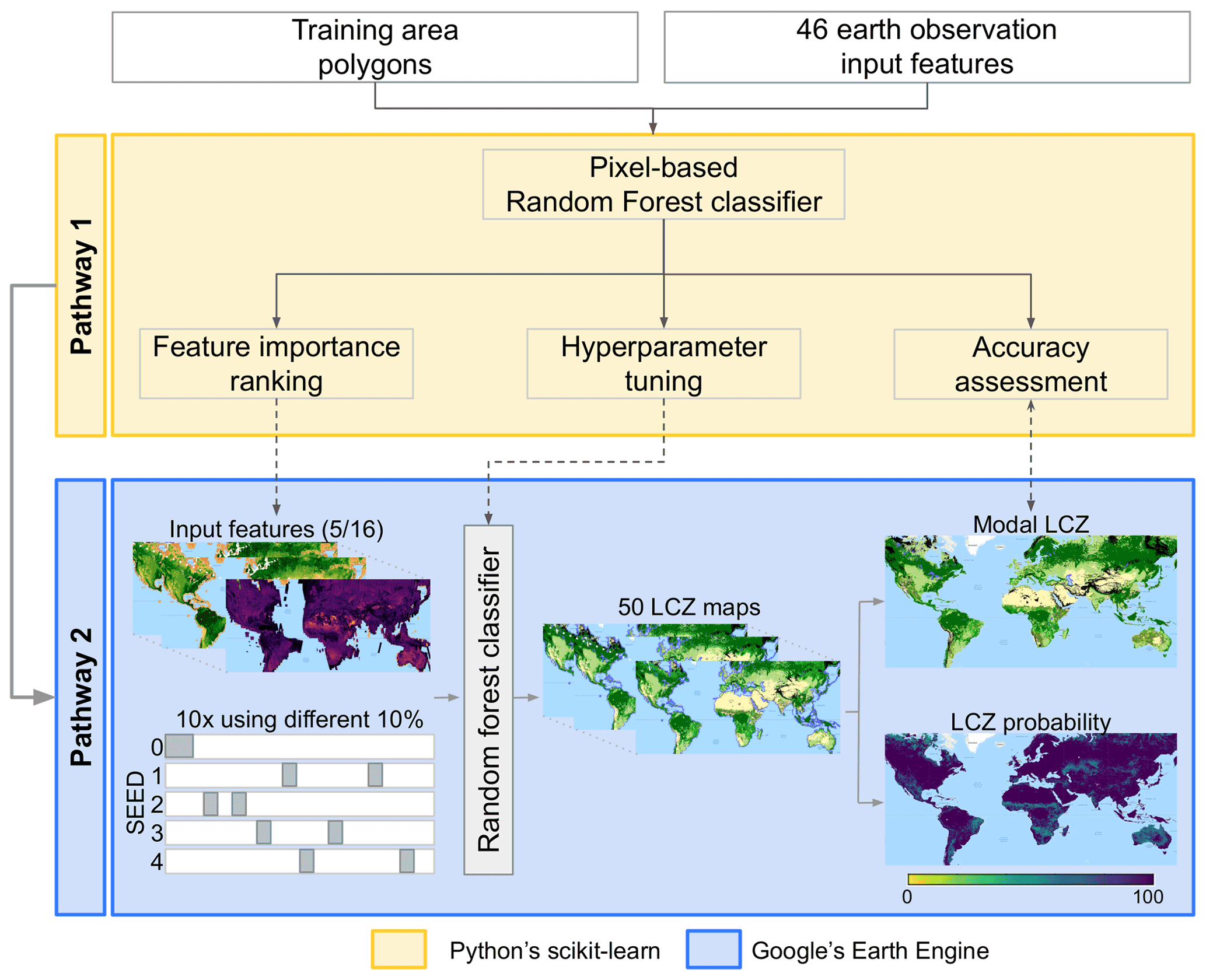
Figure 2Schematic representation of the sequential pathways to develop the global LCZ map.
In a first pathway, earth observation data are extracted from all input features and for all pixels embedded within the training area polygons. Then, using Python's random forest from the scikit-learn 0.24.2 package (Pedregosa et al., 2011) and the RF parameters used in previous work by Demuzere et al. (2019b, a, 2020a, 2021), a feature importance ranking is performed on all 46 earth observation input features for the global TA set and 15 distinct TA sets stratified by urban ecoregion. Simultaneously, the quality of these random forest classifications is assessed (see Sect. 2.4 for more information) by bootstrapping the classification 25 times, for the global TA set and the 15 urban ecoregions, each time using a stratified (LCZ class) random TA sampling of 70/30 % for training/testing. In addition, a hyperparameter tuning on EE's random forest parameters (e.g. number of trees, maximum number of leaf nodes in each tree, minimum leaf population) was applied using Python's RandomSearchCV and GridSearchCV (Pedregosa et al., 2011) packages (not shown). However, as the effect of different random forest parameters on the overall accuracy was insignificant, the default random forest parameters were kept in pathway 2.
The second pathway ingests the results from the first pathway to develop multiple lightweight global random forest models within EE. First, the reduced final input feature set is composed of the input features that belong at least 5 times (out of 16, reflecting the global and 15 urban ecoregions) to the top 50 % of the most important features obtained in pathway 1. Second, TA polygons are sampled in a double cross-folding manner, using five seeds (random samples) and 10 % of all selected TA samples (Sect. 2.1). This is repeated 10 times, each time extracting a different 10 % from the corresponding seed, resulting in 50 LCZ labels per pixel. Note that this random sampling is balanced across LCZ labels and urban ecoregions, a sampling approach that meets the three criteria as outlined by Corbane et al. (2021) and Xu et al. (2021): class balance, diversity, and representativeness. In a final step, the modal LCZ class is selected as the final LCZ label, and the resulting global modal LCZ map is post-processed using the morphological Gaussian filter described in Demuzere et al. (2020a) and Demuzere et al. (2021). In addition, a classification probability layer is produced that identifies how often the modal LCZ was modelled per pixel (e.g. a classification probability of 60 % means that the modal LCZ class was mapped 30 times out of 50 LCZ models).
2.4 Quality assessment and benchmarking
2.4.1 Traditional quality assessment
In order to assess the quality of the global LCZ map, the accuracy assessment from pathway 1 is repeated in pathway 2 using the final selected earth observation features only. Also here, the pixel-based random forest classification is repeated 50 times (5 seeds × 10 distinct TA samples), and for each iteration, the TA sample is randomly split in a balanced manner (by urban ecoregion and LCZ class) using 70/30 % for training/testing. In order to avoid spatial autocorrelation that can lead to inflated accuracies, the “splitting the polygon pool” approach is used (Xu et al., 2021), in which the polygons (rather than the individual pixels) are randomly sampled into 70/30 training/testing groups. The quality assessment is done using a range of well-accepted LCZ accuracy metrics, including overall accuracy (OA), overall accuracy for the urban LCZ classes only (OAu), overall accuracy of the built versus natural LCZ classes only (OAbu), a weighted accuracy (OAw), and the class-wise metric F1 (Chinchor, 1992; Bechtel et al., 2017; Verdonck et al., 2017; Demuzere et al., 2019b, a; Bechtel et al., 2020). The overall accuracy denotes the percentage of independent test pixels that were assigned the same class as the test label. OAu reflects this percentage for the urban LCZ classes only, and OAbu is the overall accuracy for the built versus natural LCZ classes only, ignoring their internal differentiation. The weighted accuracy (OAw) is obtained by applying weights to the confusion matrix and accounts for the (dis)similarity between LCZ types (Bechtel et al., 2017, 2020). As such, confusion between dissimilar types (e.g. LCZ 1 A) is penalized more than confusion between similar classes (e.g. LCZs 1 and 2). The class-wise accuracy is evaluated using the F1 metric, which is a harmonic mean of the user's and producer's accuracy (Chinchor, 1992; Verdonck et al., 2017). It is important to note that these accuracy metrics reflect the consistency of the TA samples but do not guarantee that the TA polygons are semantically correct. However, since a huge TA database from various sources and cities was used, this gives much more confidence than using a TA set for a single city.
2.4.2 Thematic benchmark
A drawback of the traditional accuracy assessment is that only pixels within TA polygons are evaluated, and those outside are not quality-controlled. In addition, high overall accuracies do not automatically mean that the resulting LCZ map is correct, as e.g. an insufficient discrimination of LCZ types in the training sample can lead to an artificially high OA. To accommodate such limitations, the resulting LCZ map can be converted to its corresponding urban canopy parameters (Table 1), which are key in urban ecosystem processes (Stewart and Oke, 2012; Oke et al., 2017; Ching et al., 2018, 2019) and offer an indirect thematic evaluation of the mapped LCZ quality. These UCP value ranges are not site-specific but are designed to be universally applicable to all cities, since they are based on data gathered from a large sample of measurement studies, modelling studies, existing land cover classifications, and urban climate literature reviews (Stewart, 2011a; Stewart and Oke, 2012), and even though this strategy gives rise to other limitations and challenges (e.g. having only indirect observations available or bumping into spatial and temporal resolution mismatches), it does reveal the holistic nature of the LCZ typology that distinguishes urban surfaces, accounting for their typical combination of micro-scale land covers and associated physical properties (Demuzere et al., 2020a).
Table 1A selection of urban canopy parameter data associated with built LCZ types, sourced from Stewart and Oke (2012). Columns represent the urban canopy parameters included in the thematic benchmark: the percentage of built (λB (%), ratio of building plan area to total plan area), impervious (λI (%), ratio of impervious plan area (paved, rock) to total plan area), and total impervious (λT (%), defined as the ratio of the sum of the building and impervious plan areas to the total plan area) surface areas, the mean height of roughness elements H (m) (geometric average of building heights), and the mean annual anthropogenic heat flux AHF (W m−2). Maximum values for H (LCZs 1 and 4a) and AHF (LCZ 10b) are not available and are arbitrarily set to 200 m and 1000 W m−2 respectively.

This approach is in line with previous regional works that used datasets available for specific regions only, such as for Europe (Demuzere et al., 2019a) or the continental United States (Demuzere et al., 2020a). For the current study, (semi-)independent, consistent, and open-source datasets with global coverage are selected that are critical for distinguishing the LCZ classes (surface cover, packing and height of roughness elements, and thermal properties) and that are ideally representative for the year 2018. The various products are described first, followed by an explanation of how the thematic benchmark is performed.
-
Surface cover is sourced from the Copernicus Global Land Cover Layers – Collection 3 (CGLCL3), a global discrete land cover map at 100 m resolution available on a yearly basis from 2015 to 2019, of which 2018 is selected (Buchhorn et al., 2020a, b). These maps describe the earth's terrestrial surface in up to 23 distinct land cover classes following the United Nations Land Cover Classification System (Di Gregorio and Leonardi, 2016). In contrast to the natural classes, which are primarily obtained via PROBA-V sensor data, the single urban class is largely identified using the World Settlement Footprint (WSF, Marconcini et al., 2020) from the DLR (German Aerospace Center), a global map of human settlements on earth for the year 2015.
-
Packing of the roughness elements can be characterized by the building (λB), impervious (λI), or total impervious (λT = λB + λI) surfaces. The recent literature reports on a variety of products that claim to represent global impervious surfaces (e.g. Gong et al., 2020; Marconcini et al., 2020; X. Zhang et al., 2020). These datasets generally adopt an urban mask approach; here we follow the European Environmental Agency's (EEA) definition of imperviousness density as “the percentage of sealed artificial surface” (European Environment Agency, 2018a). In contrast, the global and high-resolution Sentinel-2-based probability of built-up areas (GHS-S2Net) provides a valuable alternative (Corbane et al., 2021). GHS-S2Net is produced using a convolution neural network architecture for pixel-wise image classification that automatically extracts built-up areas at a spatial resolution of 10 m from a global composite of Sentinel-2 imagery (Corbane et al., 2020) representative for 2018. The dataset reports on built-up areas in the form of probabilities, indicating the probability of a pixel (values between 0 and 100) belonging to the built-up class. Moreover, based on an evaluation using building footprints from 277 regions across the globe (Corbane et al., 2019), Corbane et al. (2021) indicated that there is a strong relationship between the output probabilities and the building densities, suggesting that the model outputs can be used as a proxy for λB. As an additional test, we regress the GHS-S2net built-up probabilities against EEA's 100 m imperviousness density (IMD, reflecting λT) and share of built-up (SBU, reflecting λB) layers for the year 2018 (European Environment Agency, 2018a, b) for the 30 largest European functional urban areas (FUAs, Schiavina et al., 2019; see also Appendix C for more information). The results (described in Appendix D) indicate that the GHS-S2net built-up probabilities on average explain > 90 % of the observed λT and λB variability, with regression slopes closer to 1 for λB. Therefore, GHS-S2net built-up probabilities are used in this study as a proxy for λB.
-
Height of the roughness elements (building height, H) data are taken from the 3D building structure data (unpublished data based on M. Li et al., 2020), a global 1 km2-resolution database of building height, building footprint, and building volume estimated for the nominal year of 2015. The data are estimated using a random forest algorithm, based on a wide range of input layers, including optical imagery (different Landsat bands), synthetic aperture radar data from Sentinel-1, derivatives of remote sensing products (such as the enhanced vegetation and normalized difference vegetation indices), and other socio-economic data (road networks, DEMs, gross domestic product, and Gini indices reflecting economic inequalities within cities). In this product, building height denotes the average height of all buildings in a pixel, weighted by the area of each building. As such, it does not consider ground surfaces (roads, parking places, etc.) and excludes other tall features such as trees. Building height is estimated only for areas (pixels) that include built-up land in the year 2015 according to the WSF data (Marconcini et al., 2020).
-
AHF is the final LCZ attribute that can be evaluated; unfortunately, there are no global databases of thermal and radiative properties of the urban fabric that can be used. Here, the recent 1 km2 global AHF dataset from Varquez et al. (2021) is selected (hereafter referred to as AH4GUC) to benchmark the global LCZ map. AH4GUC is a freely available database (Varquez et al., 2020), contains maps of hourly and annual mean anthropogenic heat emissions representing the periods 2010s and 2050s (2010's annual mean is used here), and integrates anthropogenic heat emissions from primary energy consumption (e.g. the industrial, agricultural, commercial, residential, and transport sectors) and metabolic processes.
The thematic benchmark is performed for 150 selected urban regions (Fig. C1), which are identified by selecting the 10 most populated FUAs per urban ecoregion that are covered by the global LCZ map. In order to compare the surface cover (built versus natural) from CGLCL3 to the LCZ map, the latter is converted into a binary product; all built LCZs (except LCZ 9 – “Sparsely built”, which is predominantly natural) are converted to a single “urban” class, and all remaining classes are considered natural. A per-pixel quality assessment is then performed for each FUA and is described in terms of the balanced accuracy (BA) – providing information about the rate of correctly classified pixels in an unbalanced setting where natural pixels are predominant compared to urban pixels – and Cohen's kappa (CK) – which compensates for random chance in the pixel assignment (Corbane et al., 2021).
As can be seen from Table 1, the benchmark UCPs λB, H, and AHF are characterized by value ranges (e.g. λB for LCZ 1 ranges between 40 % and 60 %), so that a one-to-one evaluation is not possible. As such, for each of the UCPs, the mapped LCZ classes are replaced by their corresponding minimum, mean, and maximum UCP values, which are then regressed against the reference products described above. As observed H and AHF products are available at a 1 km2 resolution, the 100 m LCZ-based minimum, mean, and maximum UCP maps and 10 m GHS-S2Net urban probabilities are all resampled to a common 1 km2 resolution. The resulting coefficients of determination (R2) and slopes are reported as measures for the LCZ-based UCP explanatory power.
3.1 Global LCZ map
Applying the TA curation procedure explained in Sect. 2.1 resulted in 410 ROIs, consisting of 63 847 polygons and 2 018 916 pixels. Their distribution between ERs varies (e.g. the number of ROIs ranging between 8 and 100: for ER 11 – “Tropical, sub-tropical grassland” and ER 8 – “Tropical, sub-tropical forest in Asia” respectively), in line with global population density patterns (Fig. 3). The number of TA polygons are well-distributed across the different LCZ classes (Fig. E1), with the lowest numbers for LCZs 7 (“Lightweight low-rise”) and 1 (“Compact high-rise”) and the highest numbers for LCZs D (“Low plants”) and 6 (“Open low-rise”). It is interesting to note that, for most LCZ classes, the biggest share of TA polygons per LCZ class and urban ecoregion comes from ROIs in ER 3 – “Temperate forest in East Asia” (Fig. E1) – even though this ER only has an average number of ROIs. This is in part caused by a small number of LCZ Generator submissions with a very high number of TAs, such as the 3000+ TAs for the larger Nanjing–Bengbu–Huai'an (People's Republic of China) submission (Pan, 2021).
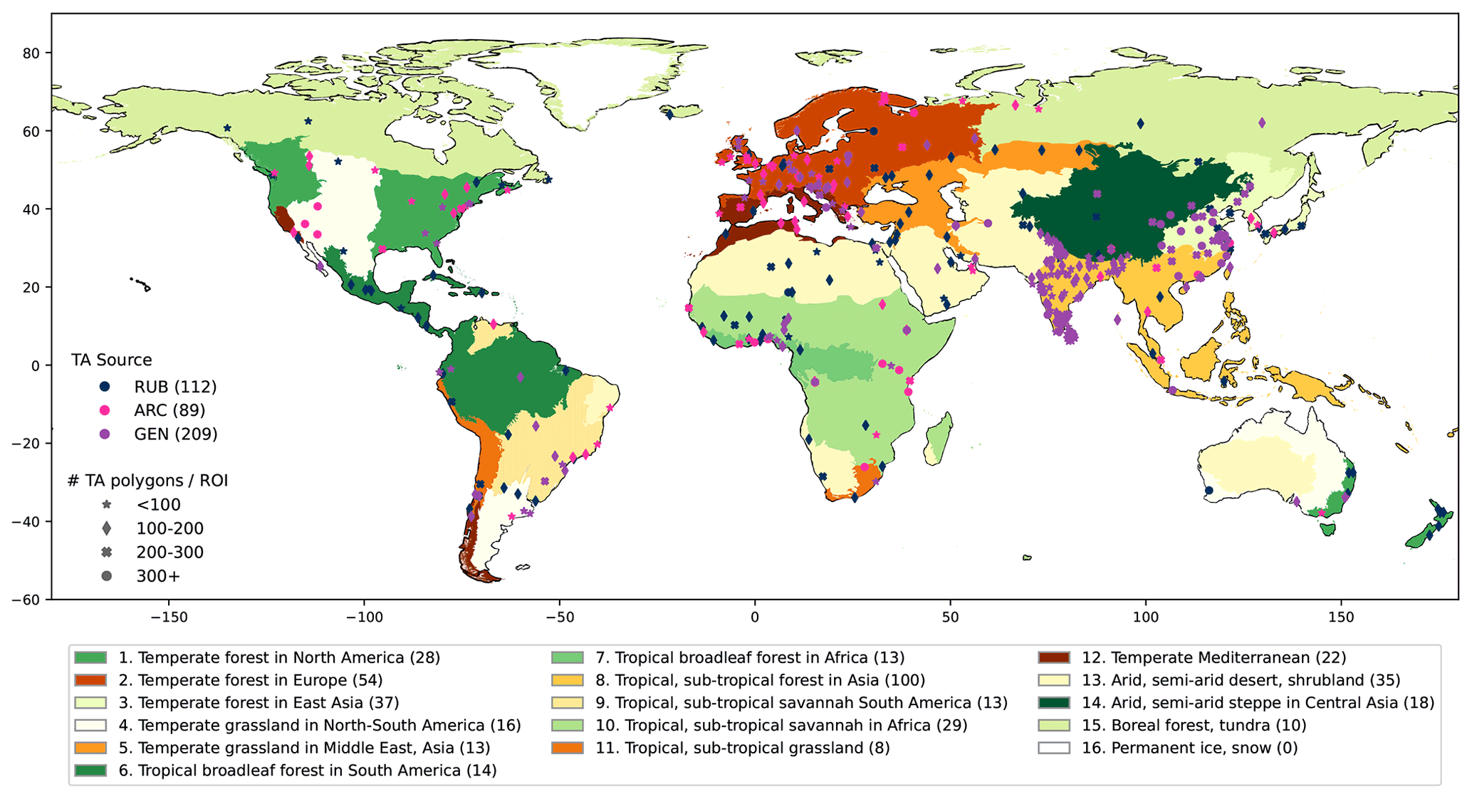
Figure 3Spatial distribution of global training area (TA) sets on top of the urban ecoregions (ERs), only showing the centroid of each region of interest (ROI). Marker type reflects the number of TA polygons per ROI, marker colours the TA source. Values between brackets in the TA source and ER legend indicate the number of ROIs per source and per ER respectively. Note that ER colours and names are adopted from Schneider et al. (2010).
Alongside the curated TA samples, 30 earth observation input features are used in the classification procedure, an outcome of the feature importance ranking procedure (Sect. 2.3). The sum average (savg) GLCM texture feature derived from PALSAR's HV polarization backscattering coefficients is found to be most important, followed by the newly developed NANTLI metric and the 90th percentile of the Normalized Difference Vegetation Index (NDVI) multi-annual composite (Fig. F1). The rest of the selected features contain information about topography, Landsat 8 bands and band ratios, Sentinel-2 NDVI band ratios, Sentinel-1 VV and VH composites, some other PALSAR HH and HV GLCM textures, and the global canopy forest height (GCFH). For clarity, a final list of selected features and their description is provided in Table F1. Finally, it is worthwhile noting that the 16 discarded features only indicate a very limited contribution to the LCZ map quality across all the urban ecoregions. For example, six features never belong to the top 50 % of the most important features (VVH, PALSAR_HH_SHADE, ASPECT, S2_sei_median, S2_csi_median, and CHM) and another five only one time (S2_B6_median, S2_B7_median, S2_rep_median, VV_HH, and EBBI) (please refer to Table 2 in Demuzere et al., 2021, for abbreviations). This indicates the generic character of the selected earth observation input feature space that is able to cover the global (urban) land surface heterogeneity representative for different clusters of climate, vegetation, and urban topologies.
The resulting 100 m spatial resolution global LCZ classification, based on all TAs and selected input features, is shown in Fig. 4. As LCZs were originally designed as a new framework for UHI studies (Stewart and Oke, 2012), they also contain a limited set of “natural” land cover classes (LCZs A to G) that can be used as “control” or “natural reference” areas, which dominate the global view. However, the seven natural classes in the LCZ scheme cannot capture the heterogeneity of the world's existing natural ecosystems and thus cannot match other products such as the 20, 36, or 75 layers that describe the earth's terrestrial surface in the Copernicus Global Land-Cover Layers (Buchhorn et al., 2020a, b), the European Space Agency Climate Change Initiative land cover map (ESA, 2017), or the global map of terrestrial habitat types (Jung et al., 2020) respectively. In contrast, the added value of the LCZ framework (and map) is the diversity of urban classes, which are easily interpretable and globally consistent, capturing the intra-urban variability of surface forms and land functions.
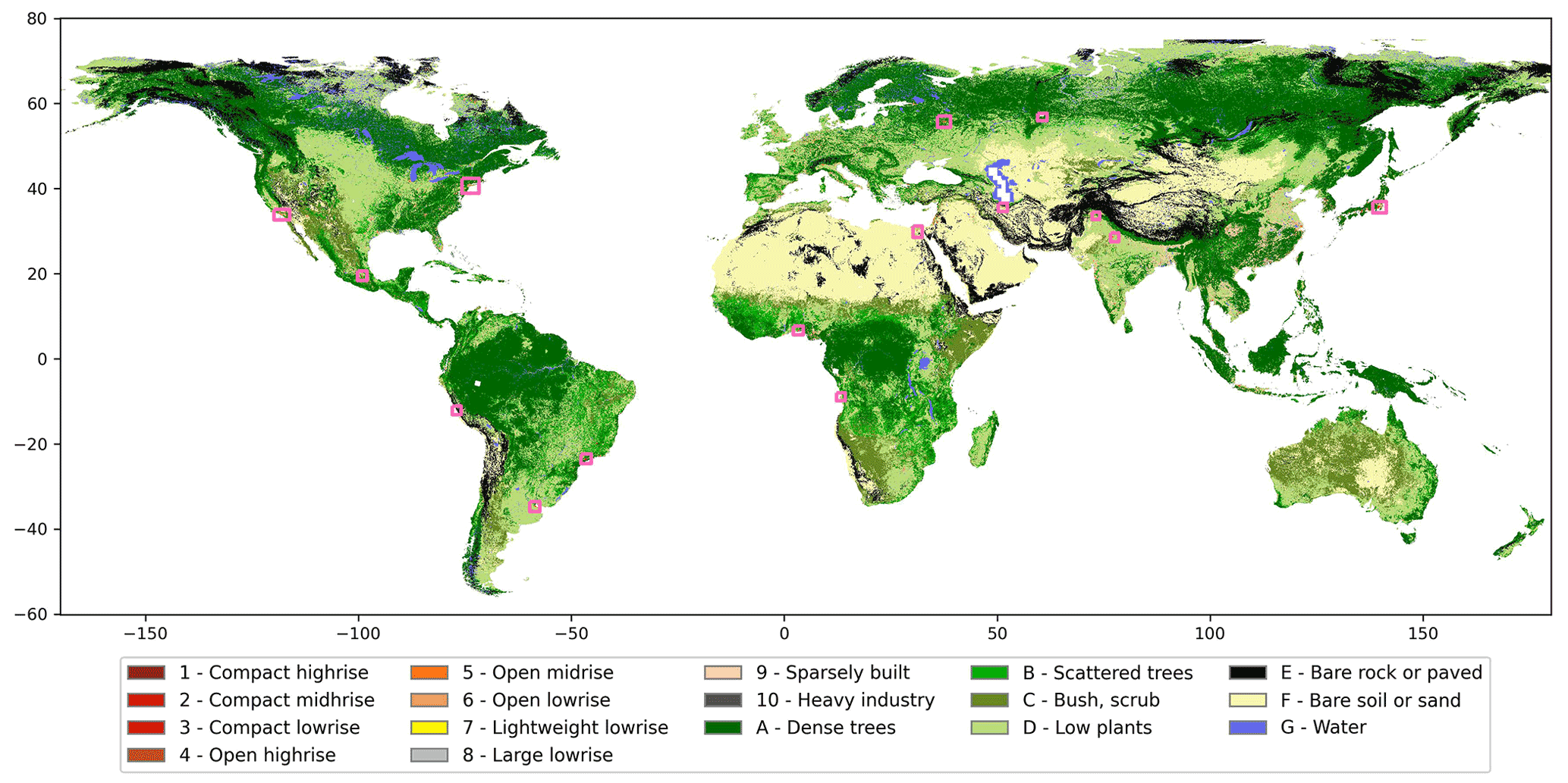
This is showcased by zooming into the largest FUAs per urban ecoregion in Figs. 5, 6, and 7, simultaneously showing the LCZ classification probabilities (discussed in Sect. 3.2) and the corresponding binary CGLCL3 surface cover. The LCZ map for e.g. New York (ER1, Fig. 5) illustrates the compact high- and mid-rise areas clustered in and around Manhattan, more open and lower-rise areas outside the city, and large-scale low-rise and industrial urban land cover around the port of Newark west of Manhattan. A second example is the city of Moscow (ER2, Fig. 5), in which its concentric layout mainly hosts LCZs 1, 2, and 4 in the centre and LCZs 5 and 6 when moving to the suburbs and its satellite cities. Such information is crucial for e.g. characterizing the UHI, as was recently demonstrated by Varentsov et al. (2020, 2021). More generally, the global LCZ map allows us to make such types of assessments for any global urban area by moving away from the traditional urban mask and incorporating cities' internal make-ups (Bechtel et al., 2017; Ching et al., 2018).
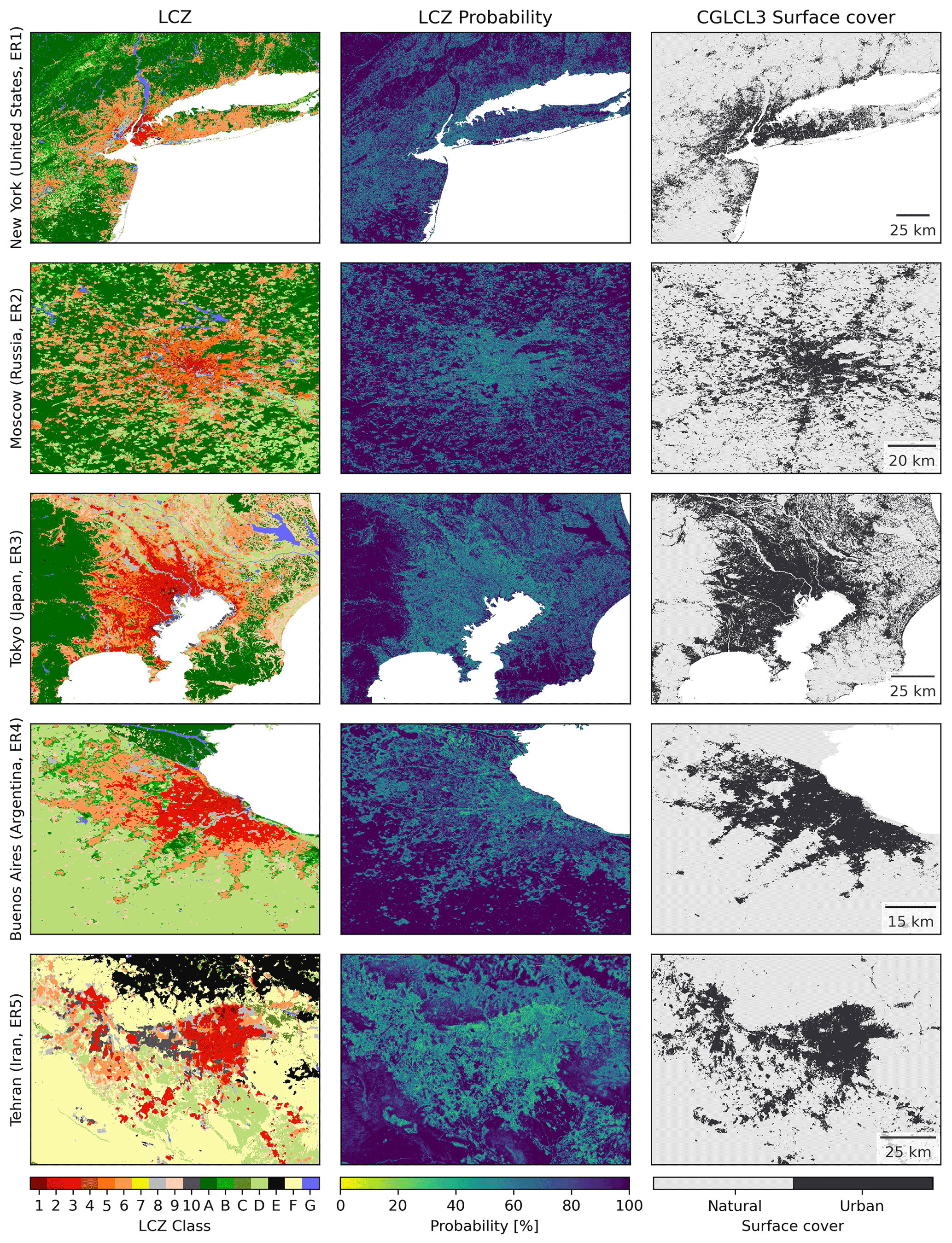
Figure 5LCZ map, its classification probability, and the corresponding binary Copernicus urban land cover (CGLCL3) for the largest functional urban areas in urban ERs 1 to 5.
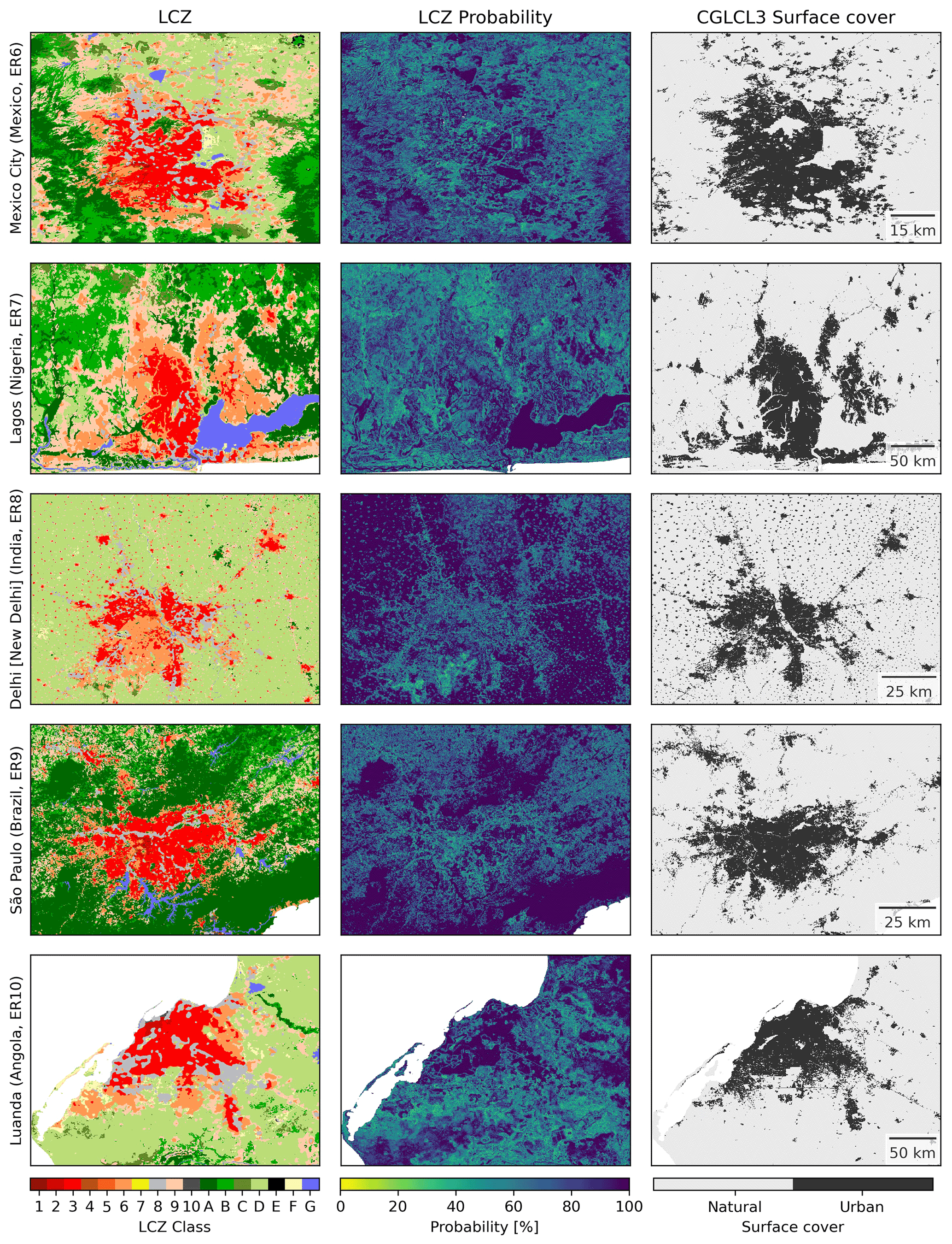
Figure 6Like Fig. 5 but for the largest functional urban areas in urban ecoregions 6 to 10.
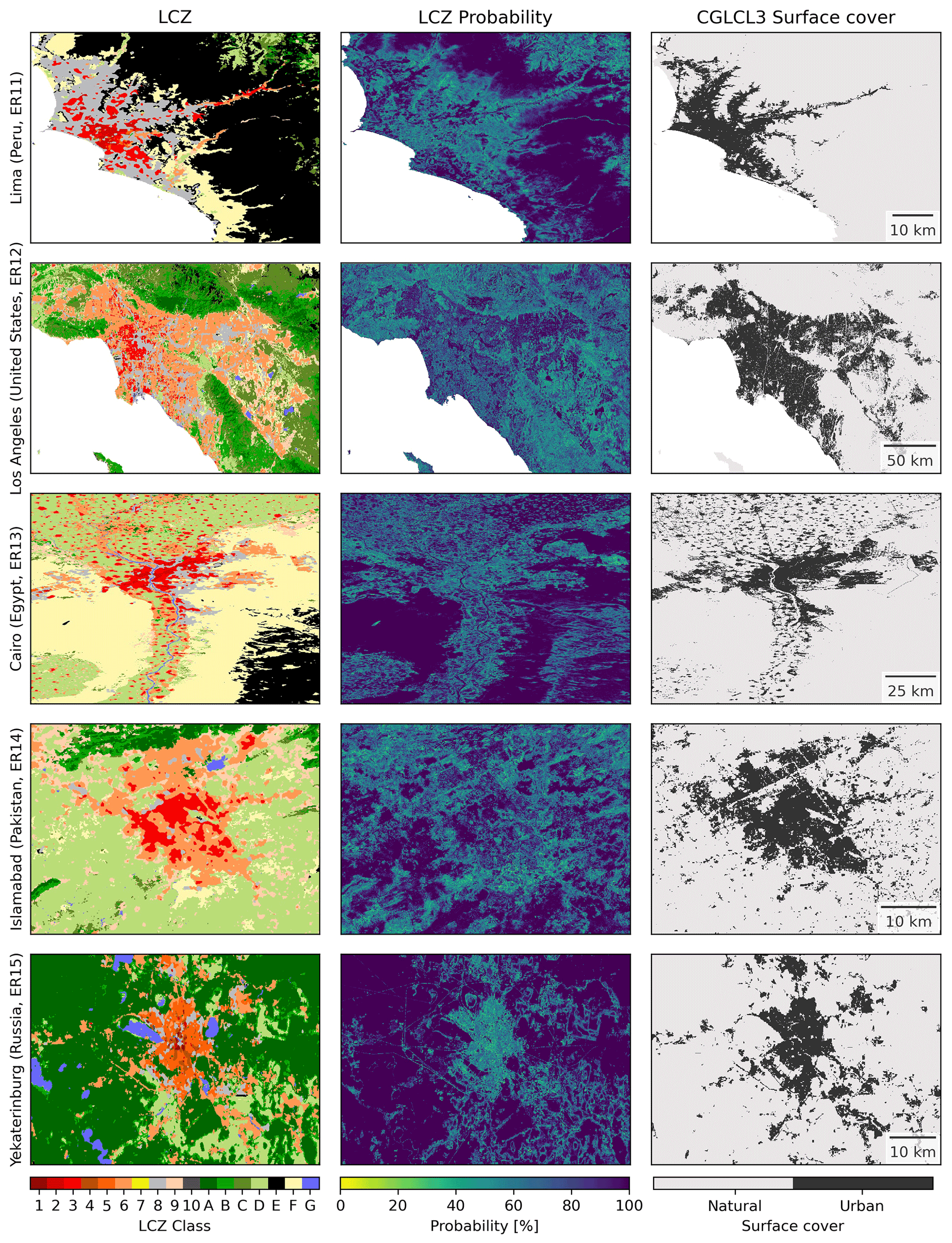
Figure 7Like Fig. 5 but for the largest functional urban areas in urban ecoregions 11 to 15.
Historic urbanization patterns are the consequence of countless decisions made at building, neighbourhood, and city scales. As such, cities have unique fingerprints reflecting distinct topographic, cultural, and economic contexts. To assess the global differences of built forms and functions, the LCZ frequencies are first categorized into groups reflecting their degree of total impervious fraction. The high-λT cluster (LCZs 1, 2, 3, and 8) is characterized by average λT > 85 %, whilst the medium-λT cluster (LCZs 4, 5, 6, and 9) typically has average λT values between 25 % and 70 %. A third cluster is added that groups LCZs 7 and 10, two LCZ classes that are distinct for their materials (LCZ 7) and anthropogenic heating (LCZ 10). The distribution of these clusters is then aggregated and visualized per urban ecoregion, enriched by their corresponding underlying LCZ classes and their building height properties (Fig. 8). It is clear that there are fundamental geographic differences in the urban layout of cities: cities in e.g. ER 1 (“Temperate forest in North America”) are dominated by the open cluster, and more specifically LCZ 6. The small fraction taken by the compact cluster is in turn dominated by LCZ 8. In contrast, cities in ER 11 (“Tropical, sub-tropical grassland”) have a more balanced distribution of compact and open classes. Here, the compact class is mostly occupied by LCZs 3 and 8 and the open cluster by LCZs 6 and 9. One consistent pattern is however apparent: a clear domination of low-rise built forms across all urban ecoregions. The two most contrasting examples in this respect are ER 3, with a relevant share of LCZs 1, 2, 4, and 5, and ER 10 (“Tropical, sub-tropical savannah in Africa”) that is almost completely dominated by low-rise built forms.
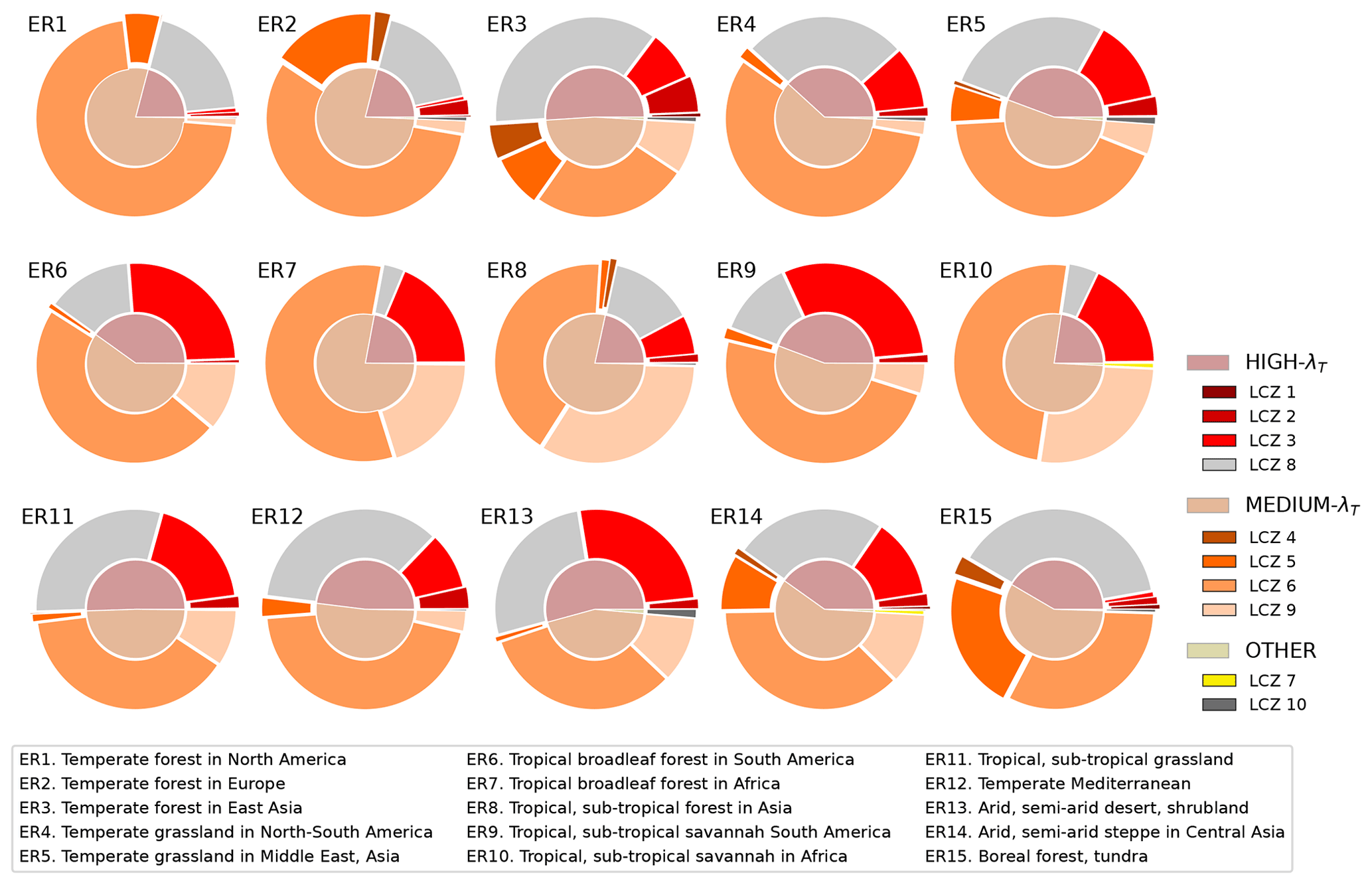
Figure 8Distribution of the built LCZ classes for all 13 135 urban centres in the Urban Centre Database, aggregated per urban ER. The inner rings indicate the HIGH (LCZs 1, 2, 3, and 8), MEDIUM (LCZs 4, 5, 6, and 9) and OTHER (LCZs 7 and 10) degree of total imperviousness (λT) clusters. The outer rings depict the actual LCZ classes. The expansion of individual LCZ wedges visually reflects the differences in building height across LCZ classes (see Table 1).
3.2 Quality assessment and benchmarking
As part of the multiple lightweight global random forest model procedure described in Sect. 2.3, a global LCZ classification probability layer is produced that identifies how often the modal LCZ was mapped (out of a total of 50 random forest results), indicating a first measure of the robustness of the classification. This classification probability layer (%) is shown in the middle panels of Fig. 5 for the largest FUAs per urban ecoregion. Yet in order to get a more comprehensive overview, LCZ-based classification probabilities are aggregated over all 13 135 cities in the Global Human Settlement Layer Urban Centres Database (GHS-UCDB, Florczyk et al., 2019) and displayed per LCZ class (Fig. 9) and ER (Fig. H1). Mean classification probabilities across the globe are greater than 50 % for all LCZ classes, meaning that the resulting modal LCZ class was mapped by more than half of the 50 LCZ models. The highest classification probability values are obtained for LCZs 6, 8, A (“Dense trees”), and G (“Water”) (∼ 80 % to 100 %), and the lowest values are found for LCZs 1, 4, 5, and 7, which can be for a variety of reasons. First, these LCZ types are typically characterized by a lower number of TAs, decreasing its potential weight in the random forest models. Second, some of these LCZ classes are characterized by similar building footprints and impervious surface areas (e.g. LCZs 4 and 5) yet differ mainly in the height of their roughness elements (see Table 1). As a conscious decision was made to use the lower-resolution building height dataset as a semi-independent benchmark dataset (described in Sect. 2.4.2), currently no input feature directly represents the roughness of buildings (see also Demuzere et al., 2019b, 2020a). In terms of the ER-stratified values (Fig. H1), all classification probabilities per LCZ class are in line with the global values, demonstrating the universality of the LCZ typology and the robustness of the classifiers and input features across the urban ecoregions. Classification probabilities for LCZ 7 deviate from this behaviour (values < 40 % for ERs 11 and 12), which might be due to the relatively low number of ROIs and the concurring lower number of TA polygons for LCZ 7. In addition, as this LCZ class includes informal settlements – often consisting of lightweight materials and densely packed buildings inter-spaced with hard-packed surfaces – these pixels present a challenge for the classifier because of their mixed spectral signature (Stewart, 2011b; Brousse et al., 2020a; Van de Walle et al., 2021, 2022). For this LCZ type, future versions of the global map might benefit and build further upon recent efforts dedicated to mapping informal urban settlements (see e.g. Kuffer et al., 2020; Assarkhaniki et al., 2021; Owusu et al., 2021; Abascal et al., 2022).
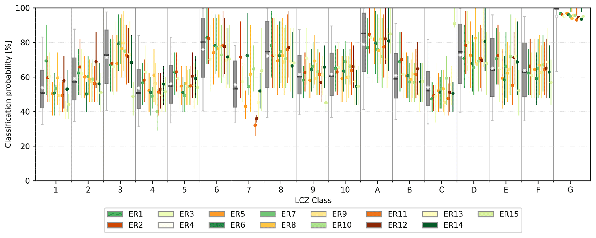
Figure 9Classification probabilities of the mapped LCZ classes, aggregated over all urban centres from GHS-UCDB. The grey boxplots depict the classification probability distribution for all global urban centres, per LCZ class, with boxes and whiskers spanning the 25th–75th and 5th–95th percentiles respectively and means and medians indicated by the white dots and black lines respectively. The vertical lines in the colours of the urban ERs (colour legend as in Fig. 3) indicate the 25th–75th percentile range averaged over the urban centres, stratified per ER. ER-coloured dots indicate the mean. Results stratified per urban ecoregion are available in Appendix H.
The traditional accuracy assessment using the independent training/test samples obtained via the “splitting the polygon pool” approach (Xu et al., 2021) and the 50 lightweight random forest models results in scores of > 70 % for all OA metrics (Fig. G1). The variability across the 50 random forest models is small, indicating the robustness of the global classification protocol. Interestingly, the global OA values using the reduced set of final input features is higher compared to the accuracy assessment using all input features (74.5 % ± 15.1, Fig. F1), supporting the valid removal of uninformative input features from the multi-dimensional input feature space. The class-wise F1 metric shows larger variability with values for the built LCZs between 50 % (LCZ 1 – “Compact high-rise”) and 78 % (LCZ 6 – “Open low-rise”) and > 60 % for all natural classes. The lowest accuracy is obtained for LCZs 1, 4, 5, 7, and 10, in line with the results of the classification probability layer discussed above.
Since the LCZ typology is a representation of urban form – defined via the corresponding universal LCZ-based canopy parameters – a thematic benchmark allows us to indirectly assess the quality of the LCZ map for continuous land surfaces, including those pixels not part of the TA samples used in the traditional accuracy assessment. Figure 10a reveals a good correspondence between the built LCZ classes and the urban class from the CGLCL3 – taken from the World Settlement Footprint data (Marconcini et al., 2020) – with an average BA and CK of 90 % and 73 % respectively. Stratifying the BA results per urban ecoregion indicates a similar performance, with mean BA values ranging between 83 % (ER3) and 93 % (ER4) (Fig. I1). A similar variability can be observed for the CK results stratified per urban ecoregion, with mean CK values ranging between 65 % (ER8) and 80 % (ER9). These results indicate that the global LCZ map presents a good correspondence to a state-of-the-art and dedicated built-up land data product and is thus able to correctly discriminate between built-up and natural land cover (confirmed independently by an OAbu of ∼ 95 %, an accuracy metric that evaluates the built versus natural LCZ classes only – Fig. G1).

Figure 10Results for the thematic benchmark, for the urban mask from the Copernicus Global Land Cover Layers (a) and the building surface fraction, building height, and anthropogenic heat flux (λB, H, and AHF respectively) (b, c). All accuracies are derived for the 150 global LCZ functional urban areas. For built-up land, accuracy is expressed using the balanced accuracy (BA) and Cohen's kappa (CK). For λB, H, and AHF, the coefficients of determination (R2) (b) and slopes (c) result from the regression between the reference datasets and their corresponding universal LCZ-based values from Stewart and Oke (2012), using minimum (Min), mean, and maximum (Max) values (colours). For all panels, boxes and whiskers span the 25th–75th and 5th–95th percentiles respectively. The means and medians are indicated by the black dots and lines respectively. Results stratified per urban ecoregion are available in Appendix I.
For λB, H, and AHF – characterized by UCP value ranges (Table 1) – a one-to-one evaluation with their reference datasets (described in Sect. 2.4.2) is not possible. As such, minimum, mean, and maximum UCP values are regressed against these reference products, from which the coefficients of determination (R2) and slopes represent the measures of the explanatory power of the LCZ map (Figs. 10b, c and I2 for results stratified per urban ecoregion). The LCZ-based building surface fraction λB is in very good agreement with the GHS-S2Net proxies, with mean R2 values close to 0.9 for the whole value range. Slope values provide a slightly more nuanced result, with average values of 0.69, 1, and 1.22 when targeting the minimum, mean, and maximum λB UCP values. In other words, assigning the means of the λB value ranges to each corresponding LCZ class is a very good approximation for the building surface fraction for global cities. Results for building heights H and the AHF can be interpreted in the same way (Figs. 10b, c and I3 and I4 for results stratified per urban ecoregion). For H, R2/slope values range between 0.42/2.5 and 0.5/0.59 for the maximum and minimum LCZ-based H values. Also here, the best results are obtained using the mean of the LCZ-based value ranges, even though only ∼ 50 % of the observed building height is explained and the mean LCZ-based values tend to overestimate the reference values. For AHF, it is clear that assigning the minimum of the LCZ-based AHF range to the LCZ map has little explanatory power: R2 is 0.1 with a slope of ∼ 0.1. Sightly better results are obtained when using the maximum and especially the mean of the AHF value range, but here only 30 % of the observed AHF variability can also be explained by the LCZ map. From previous anthropogenic heat flux works (Oke et al., 2017), it is clear that this is not surprising. The AHF values provided by Stewart and Oke (2012) are fixed ranges, reflecting the mean annual heat flux density from fuel combustion and human activity (transportation, space cooling/heating, industrial processing, human metabolism) at the local scale. Yet, as also indicated in their Table 4 (footnote c), these values vary significantly with latitude, season, and population density. LCZs have previously been shown to indirectly capture information on population densities (Demuzere et al., 2020a), and the role of seasonality with respect to LCZ-based annual AHF values has also been discussed elsewhere (e.g. Varentsov et al., 2020). Yet it is obvious that the observed zonal AHF variability in AH4GUC (Varquez et al., 2021, their Fig. 5) is neglected completely in this thematic benchmark. This means that, for example, an LCZ 6 neighbourhood in tropical Singapore will be assigned the same mean annual AHF values as an LCZ 6 area in the high-latitude city of Helsinki (Finland), even though it is clear that their building cooling/heating patterns will be completely different (Quah and Roth, 2012; Karsisto et al., 2016). This reveals a strong limitation of using AHF as an independent benchmark of the global LCZ map. Unfortunately, as there are currently no globally explicit databases on thermal and radiative properties of the urban fabric, AHF is currently the only available proxy to indirectly assess the “thermal” signature of a built environment. Finally, there are a number of other elements that might affect deviations between the LCZ-based UCP parameters and their benchmark products and comparison methods: some benchmark products are merely indirect observations (e.g. GHS-S2Net urban probabilities being used as a measure for λB), and UCPs might have dissimilar definitions (e.g. the geometric average of buildings heights versus the average of building heights weighted by the building footprint) or data matching differences as a consequence of different resolutions and map projections leading to potential artefacts from resampling.
Despite the new focus on cities as a critical scale for climate change risk management, we know very little about most cities on the planet – being generally ignorant of their extent, how they are constructed, and how they are occupied (Demuzere et al., 2020a). This knowledge gap is especially true for urban areas in low- and middle-income countries, where 90 % of the projected world population growth of 2.5 billion over the next couple of decades will occur. This is in strong contrast to current urban knowledge, which is predominantly shaped by research on and from high-income countries (Nagendra et al., 2018). The global local climate zone map presented here provides a globally consistent and climate-relevant urban description, which is an important prerequisite for developing fit-for-purpose integrated climate-sensitive urban planning policies (Georgescu et al., 2015). As LCZs are developed from generalized perspectives of built forms and land cover types that are universally recognized and applicable (Stewart and Oke, 2012), this global LCZ map provides standardized and harmonized data of all cities, allowing us to consistently assess the heterogeneous nature of cities' urban forms and functions and providing the much-needed platform for comparative analyses, systematic learning, and horizontal knowledge exchange between cities and regions (Raven et al., 2018; Ching et al., 2018; Bai et al., 2018; Creutzig et al., 2019; Reba and Seto, 2020).
As cities are complex systems and their components are difficult to understand in isolation, scaling – a general analytical framework used by many disciplines – is often put forward to understand and describe cities' dynamics, growth, and evolution in scientifically predictable, quantitative, and universal laws (Bettencourt et al., 2007, 2020). Some works for example represent city growth, structures, and functions (e.g. urban area, albedo, population density, building density, building heights, anthropogenic heat flux, and sky view factor) completely by population (Schläpfer et al., 2015; Manoli et al., 2019; Martilli et al., 2020). Other work has explored the correspondence between population density and carbon dioxide emissions (Ribeiro et al., 2019) and the allometric-scaling relationships between settlement populations and non-point-source emissions of air pollutants (MacKenzie et al., 2019). In reality, the global universality of these scaling laws is unknown, as many are created based on regional information only, mostly for data-rich parts of the world (Bettencourt and West, 2010). Currently, city population is often used as a proxy for urban form (e.g. Schläpfer et al., 2015; Manoli et al., 2019), but the global LCZ map offers a richer alternative. In addition, the combination of population and LCZ may provide deeper insights into the variations of form in different cultural, socioeconomic, and climatic contexts and help guide future urban development. Since LCZs distinguish urban areas based on their form, the global map provides the means to assess the universality of the above-mentioned scaling laws and refine/improve them. In addition, the global LCZ map has value beyond climate applications when combined with other spatially resolved urban information (Reba and Seto, 2020), like flooding hazard, biodiversity, and air quality.
Since the LCZ typology was initially designed for urban temperature studies (Stewart and Oke, 2012), typical applications focus on the UHI, usually providing the context for designing and analysing observations from urban meteorological networks (Skarbit et al., 2017; Beck et al., 2018; Chieppa et al., 2018; Verdonck et al., 2018; Yang et al., 2018; Leconte et al., 2020; Milošević et al., 2021; Y. Zhang et al., 2020; Zong et al., 2021), from crowd-sourced data (Fenner et al., 2017; Varentsov et al., 2021; Fenner et al., 2021; Potgieter et al., 2021; Brousse et al., 2022), or from remote sensing (Wang and Ouyang, 2017; Bechtel et al., 2019b; Eldesoky et al., 2021; Stewart et al., 2021). However, the typology has been used for other purposes (see also Lehnert et al., 2021, for European applications), such as urban heat (risk) assessment studies (Verdonck et al., 2019b; Van de Walle et al., 2022), climate-sensitive design, land use/land cover change, urban planning (policies) (Perera and Emmanuel, 2018; Aminipouri et al., 2019; Vandamme et al., 2019; Maharoof et al., 2020; Chen et al., 2021b; Zhi et al., 2021), anthropogenic heat, building energy demand and consumption, carbon emissions (Wu et al., 2018; Santos et al., 2020; Yang et al., 2020; Benjamin et al., 2021; Kotharkar et al., 2022), quality of life (Sapena et al., 2021), urban ventilation (Z. Zhao et al., 2020), air quality (Steeneveld et al., 2018; T. Lu et al., 2021), urban vegetation phenology and ecosystem patterns, functions, and dynamics (Kabano et al., 2021; Zhao et al., 2022), and epidemiological studies (Brousse et al., 2019, 2020a).
The LCZ scheme is a core element of the WUDAPT project to provide consistent urban data to support climate science (Ching et al., 2018, 2019), and many modelling systems nowadays ingest the LCZ typology, such as e.g. the Surface Urban Energy and Water Balance Scheme (SUEWS, Alexander et al., 2015, 2016), UrbClim (Verdonck et al., 2018, 2019b; Sharma et al., 2019; Gilabert et al., 2021), the Vertical City Weather Generator (Moradi et al., 2022), ENVI-met (Middel et al., 2014; Lyu et al., 2019; Bande et al., 2020), the urban multi-scale environmental predictor (UMEP, Lindberg et al., 2018), MUKLIMO_3 (Bokwa et al., 2019; Matsaba et al., 2020; Gál et al., 2021), COSMO-CLM and the WUDAPT-TO-COSMO tool (Wouters et al., 2016; Brousse et al., 2019, 2020b; Varentsov et al., 2020; Van de Walle et al., 2021), the Weather Research and Forecasting model (WRF, Brousse et al., 2016; Hammerberg et al., 2018; Molnár et al., 2019; Pellegatti Franco et al., 2019; Wong et al., 2019; Mu et al., 2020; Zonato et al., 2020; Patel et al., 2020; Hirsch et al., 2021; Patel et al., 2022), and the WUDAPT-TO-WRF tool (Demuzere et al., 2022c). Most studies focus on individual cities, with the work of Patel et al. (2022) being an exception as it uses the European LCZ map (Demuzere et al., 2019a) to simulate a continental-scale heat wave event. The LCZ map presented here allows the extraction of urban data suited to the scale of study and can support global climate and earth system modelling.
Regional climate models are expected to remain indispensable tools that complement global models for understanding physical processes governing regional climate variability and change (Gutowski et al., 2020). Yet at the same time regional climate model developments also serve as precursors for the evolution of global climate models, and major efforts are currently under way to increase ESMs to kilometre-scale resolutions (Schär et al., 2020; Bauer et al., 2021). Recently, Fuhrer et al. (2018) performed a near-global climate simulation at a horizontal grid spacing of just 930 m. Such advancements will represent a quantum leap in (urban) global climate modelling, enabling the explicit treatment of the complex interactions between the fine-grained urban heterogeneity and its atmosphere (Martilli et al., 2020). To date, however, climate projections focused on built landscapes are absent, partly owing to the lack of climate-relevant urban data for ESMs (Zhao et al., 2021; Hertwig et al., 2021). Only one ESM included details of urban form in CMIP51 (Zhao et al., 2021) and a few more in CMIP6: except for GFDL-ESM (Dunne et al., 2020), these CMIP6 ESMs all use the Community Land Model-Urban (CLMU) canopy parameterization (Oleson and Feddema, 2020). Yet despite its pole position, CLMU's lead developers indicate that transitioning to the LCZ urban classes and their corresponding UCPs will likely be beneficial for better simulating the interactions between the urban fabric and the climate system (Oleson and Feddema, 2020). Eventually, a closer connection between the global LCZ map and the ESM community might have a direct impact on climate change policies via the IPCC's2 upcoming 7th cycle of Assessment Reports and its planned Special Reports on Cities and Climate Change.
Even though the LCZ typology presents a leap forward in describing intra-urban heterogeneity in a universal manner, its generalization of course also has its limitations. In the words of Stewart and Oke (2012), “its view of the landscape universe is highly reductionist […] and LCZs represent a simple composition of buildings, roads, plants, soils, rock, and water, each in varying amounts and each arranged uniformly into 17 recognizable patterns. The 17 patterns should nevertheless be familiar to users in most cities, and should be adaptable to the local character of most sites”. This multi-urban class typology follows the discourse of most categorical mapping efforts discussed elsewhere (Coops and Wulder, 2019), such that individual LCZ classes are all physically discrete in surface structure and land cover, leading to well-defined boundaries separating most classes. However, users of LCZs must always accept that the internal homogeneity portrayed by each class is unlikely to be found in the real world but that the attempt to classify surface complexity in cities represents a key advancement in urban climate science (Stewart and Oke, 2012). It also represents a helpful starting point for more detailed studies of urban form and function at smaller spatial scales. Likewise, due to its reductionist character, the landscape universe represented by the 17 LCZ classes is not complete for several reasons. First, we do not apply LCZ sub-classes that represent combinations of built types, land cover types, and land cover properties (Stewart and Oke, 2012), allowing for a mixture of several LCZ types but reducing its universality. Secondly, some landscapes such as extensive greenhouses are not included in the scheme, since they are unlikely to be selected for urban heat island studies. Moreover, the scale of real urban structures does not always match the climatic definition of local scales. However, we are convinced that the scheme is the best compromise between climatic variation and generic description of urban structures.
This first version of the global LCZ map itself also has limitations. For example, LCZ 7 requires more attention and alternative mapping strategies, as discussed in Sect. 3.2. Confusion may also exist between classes with similar impervious and built-up surface fractions characterized by similar spectral characteristics (not shown), which can lead to confusion between these classes (see e.g. the confusion between LCZs 3 and 8 in the LCZ map for Lima (Peru, ER11), Fig. 7). Similarly, the confusion between classes with similar surface fractions yet different heights of roughness elements might also be improved in the future. More generally, the results of the thematic benchmark reveal that two-dimensional information (urban land cover and building surface fractions) is well-represented but that the corresponding three-dimensional (3D) information requires more attention. Ongoing developments such as the work on the Digital Synthetic City (Ching et al., 2019), tailored towards providing more detailed information on the urban landscape (WUDAPT Levels 1 and 2), or global 3D building information (M. Li et al., 2020; Esch et al., 2022; Kamath et al., 2022) might contribute to improving the quality of future LCZ map releases. It is also important to note that the LCZ map also inherits shortcomings of the many global earth observation input features upon which it is built, such as some missing data in areas that are frequently covered in clouds or gaps in coverage because of changing satellite duty cycles. Such limitations can be addressed in future releases of the map, e.g. by harvesting the growing number of TA samples submitted to the LCZ Generator (which received more than 1500 submissions in less than 1 year of operation), ingesting more and new high-resolution (earth observation) datasets when available, or implementing alternative scalable classification algorithms (e.g. Yokoya et al., 2018; Yoo et al., 2020; Rosentreter et al., 2020). Nevertheless, from the many above-mentioned examples and applications it is clear that this global LCZ map has a lot of potential, serving urban and climate sciences at various scales. The map is universal and allows for comparisons between global regions. Yet at the same time it is flexible enough to allow anyone to adapt it to suit their purpose, using for example user- and site-specific LCZ-based UCP values if available (Ching et al., 2018). In other words, the global LCZ map describes all the cities of the world in the same, universal language, but interested users can read it in their own dialect. In addition, interested users are invited to actively contribute to future releases of this product by submitting city-specific training area sets to the LCZ Generator. This community engagement will not only improve the quality of the next LCZ map releases, but will also contribute to the overall WUDAPT philosophy to provide urban canopy information and modelling infrastructure to facilitate urban-focused climate, weather, air quality, and energy-use modelling application studies (Ching et al., 2018). Finally, this development will also support future large-scale dynamic LCZ mapping efforts. Such examples to date are rare and focus on targeted cities (e.g. Vandamme et al., 2019; Wang et al., 2019; Demuzere et al., 2020b; C. Zhao et al., 2020; Y. Lu et al., 2021; Zhi et al., 2021), yet they reveal large potential in terms of characterizing the temporal transformations of urban morphologies across and within different cities, identify the main drivers of such changes, and bridge the gap between policy-making and urbanization patterns required to come up with informed, data-driven, and rational urban planning strategies toward sustainable city developments.
The global local climate zone map, representative for the nominal year 2018 and with a spatial resolution of ∼ 100 m (EPSG:4326), is available from https://doi.org/10.5281/zenodo.6364594 (Demuzere et al., 2022a). The dataset contains various layers stored as separate GeoTIFF files, including (1) lcz_filter, the recommended global LCZ map after applying the morphological Gaussian filter described in Demuzere et al. (2020a), (2) lcz, like (1) but presenting the raw LCZ map before applying the morphological Gaussian filter, and (3) the LCZ classification probability layer (%) that identifies how often the modal LCZ from (2) was chosen per pixel. The LCZ maps have the default WUDAPT LCZ colour scheme embedded (Fig. 1), and all imagery can be processed using (free) GIS software, e.g. QGIS. In addition, a teaser sample is provided to ease accessibility, providing the LCZ map information for the 15 largest functional urban areas stratified by urban ecoregion. These GeoTIFF files reflect the underlying data used in Figs. 5, 6, and 7 of the paper. This teaser dataset is available from https://doi.org/10.5281/zenodo.6364705 (Demuzere et al., 2022b).
Since their introduction in 2012, local climate zones (LCZs) have become a standard for characterizing urban landscapes according to climate-relevant properties of the surface. From that point forward, the number of applications using this universal urban typology has been growing exponentially, revealing the relevance and potential for a wide range of urban sciences. One of the typology's most popular uses is digital mapping, which can generate UCPs at the city scale for input to numerical climate models. However, the lack of available and consistent global data on the form and function of cities has impeded progress in urban climate sciences so far, limiting applications to cities or regions for which LCZ maps are currently available.
The 100 m-resolution global LCZ map presented here is the first of its kind depicting the much needed global intra-urban heterogeneity in a universal language. It allows easy access to local climate zone data for regional- and global-scale analysis and provides a seamless integration into existing topographic, natural land cover, and other global-scale data products. The map is generated by building further upon previous studies whilst adding new methodological features that balance optimal learning across global climates and urban typologies with accuracy, computational feasibility, and efficiency.
Since this global map identifies the relevant data for planning and climate on neighbourhood, city, and global scales, it is designed to become part of a basic infrastructure to support a host of studies on exposure to environmental hazards, energy demand, climate adaptation, and mitigation solutions and human health, as examples.
In order to guide a user in the digitization of LCZ training area polygons, a set of digitization guidelines is provided on the WUDAPT web page (https://www.wudapt.org/digitize-training-areas/, last access: 22 August 2022). This information is split into two parts, discussing (1) how to digitize a LCZ polygon using Google Earth and the provided .kml template, and (2) good-practice guidelines for digitization (Fig. A1).
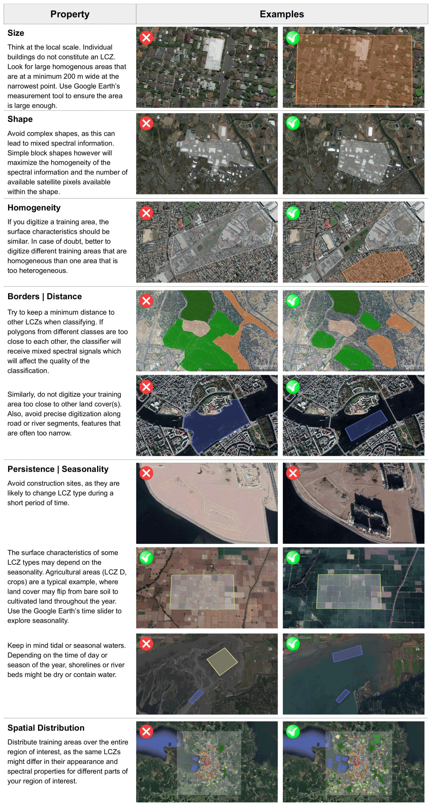
Figure A1Good-practice guidelines for digitizing LCZ training area polygons (© Google Earth 2020).
To date, very few studies have tested the added value of texture features (derived from the Gray-Level Co-occurrence Matrix, GLCM) in the LCZ classification procedure. Forget et al. (2018) found that combining features computed from both Sentinel-1 VV and VH backscatter polarizations consistently led to better LCZ classification performances in 12 sub-Saharan African urban areas, even though the introduction of textures computed from different spatial scales did not improve the classification performances. Along the same lines, Hu et al. (2018) found that Sentinel-1 dual-Pol SAR data (including texture features) can contribute to the classification of transcontinental cities into several LCZ classes. Also, Brousse et al. (2020a) successfully used Sentinel-1 GLCM texture features with an 11-by-11 kernel window size to map nine sub-Saharan African urban areas, in order to better capture the heterogeneities of built-up surfaces.
Since Sentinel-1 backscatter information is already available in the input feature space, and inspired by the findings of Hay Chung et al. (2021), PALSAR (Phased Array type L-band Synthetic Aperture Radar, Shimada et al., 2014) backscattering information was added, though not the pure HH and HV backscatter information as in Hay Chung et al. (2021), but rather the GLCM texture features derived from them (Haralick et al., 1973; Conners et al., 1984; Chen et al., 2021a), as follows.
-
A median 2017–2019 PALSAR composite is created for both the HH and HV polarization backscattering coefficients.
-
For each polarization, the 18 GLCM texture features are derived, with 2-by-2 and 4-by-4 kernel windows, corresponding to 50 and 100 m spatial resolutions respectively.
-
Only the contrast, dissimilarity, inertia, sum average, and cluster shade texture measures are retained, as the remaining textures indicated little added value in the LCZ mapping (not shown).
In addition, the Visible Infrared Imaging Radiometer Suite (VIIRS) Day/Night Band (DNB), provided by Mills et al. (2013), was also used as follows.
-
A median 2017–2019 composite is created from the monthly VIIRS Stray Light Corrected Nighttime Day/Night Band Composites (NTL).
-
This median NTL image is smoothed with a convolution filter using a radius of 300 m.
-
Afterwards, the smoothed NTL image is normalized (hereafter referred to as NTLnorm).
-
NANTLI is calculated, a Normalized Difference Vegetation Index (NDVI)-adjusted NTL index, according to Eq. (B1).
Note that NANTLI is analogous to EANTLI (Zhuo et al., 2015) yet uses the Landsat 8 NDVI input feature available from Demuzere et al. (2021) instead of the EVI (Enhanced Vegetation Index), introduced to mitigate both saturation problems and blooming effects of VIIRS data (Zhuo et al., 2018; X. Zhang et al., 2020).
The added values of these features are evaluated by mapping 45 cities (3 cities per urban ecoregion, characterized by large TA samples with a large number of different LCZ classes) into LCZs, following the procedure of the LCZ Generator (Demuzere et al., 2021) but each time using a different set of earth observation input features. This results in four experiments.
-
GEN: the default 33 input features available from the LCZ Generator
-
GEN+NANTLI: GEN and NANTLI
-
GEN+NANTLI+P2: GEN, NANTLI, and the PALSAR texture features derived with kernel size 2-by-2
-
GEN+NANTLI+P4: GEN, NANTLI, and the PALSAR texture features derived with kernel size 4-by-4
Results are evaluated in terms of the overall accuracy metrics (OAs) described in Sect. 2.4. Figure B1a displays the OAs for the GEN experiment for each individual city sorted by urban ecoregion (ERs 1–15). Figure B1b, c, and d indicate the change in OAs for GEN+NANTLI, GEN+NANTLI+P2, and GEN+NANTLI+P4 respectively compared to GEN. Adding NANTLI increases the average OAs between 0.3 % and 2 %, with individual city values ranging between −1 % and 5.8 % (for Constantine, ER12, and Cologne, ER2, respectively). Adding PALSAR texture features further increases the average OAs between 0.8 % and 3.2 % (GEN+NANTLI+P2, Fig. B1C) and between 0.9 % and 3.8 % (GEN+NANTLI+P4, Fig. B1d). Here, individual city values range between −0.3 (Itanagar, ER14) and 7.8 % (Rosario, ER4) for GEN+NANTLI+P2 and between −0.9 (Havana, ER6) and 13.8 % (Rosaria) for GEN+NANTLI+P4. As such, the VIIRS-based NANTLI input feature together with the PALSAR-based GLCM texture features, using a 4-by-4 kernel size, are selected as an additional earth observation for the LCZ mapping procedure.
Figure B1Overall accuracies for the various input feature experiments: absolute overall accuracies for all cities for GEN (a) and differences in overall accuracies for experiments GEN+NANTLI (b), GEN+NANTLI+P2 (c), and GEN+NANTLI+P4 (d) compared to GEN. Numbers on the top x axis indicate the average overall accuracy (change) across all cities. ER refers to urban ecoregion.
Functional urban areas (FUAs), as defined by the Organisation for Economic Co-operation and Development (OECD) and the European Union, are sets of contiguous local (administrative) units composed of a city and its surrounding, less densely populated local units that are part of the city's labour market (commuting zone). As such, these units not only offer the opportunity to evaluate more densely built city centres, but also their sparsely built or natural neighbouring landscapes. The 10 most populated FUAs per urban ecoregion used in the thematic benchmark are depicted in Fig. C1.
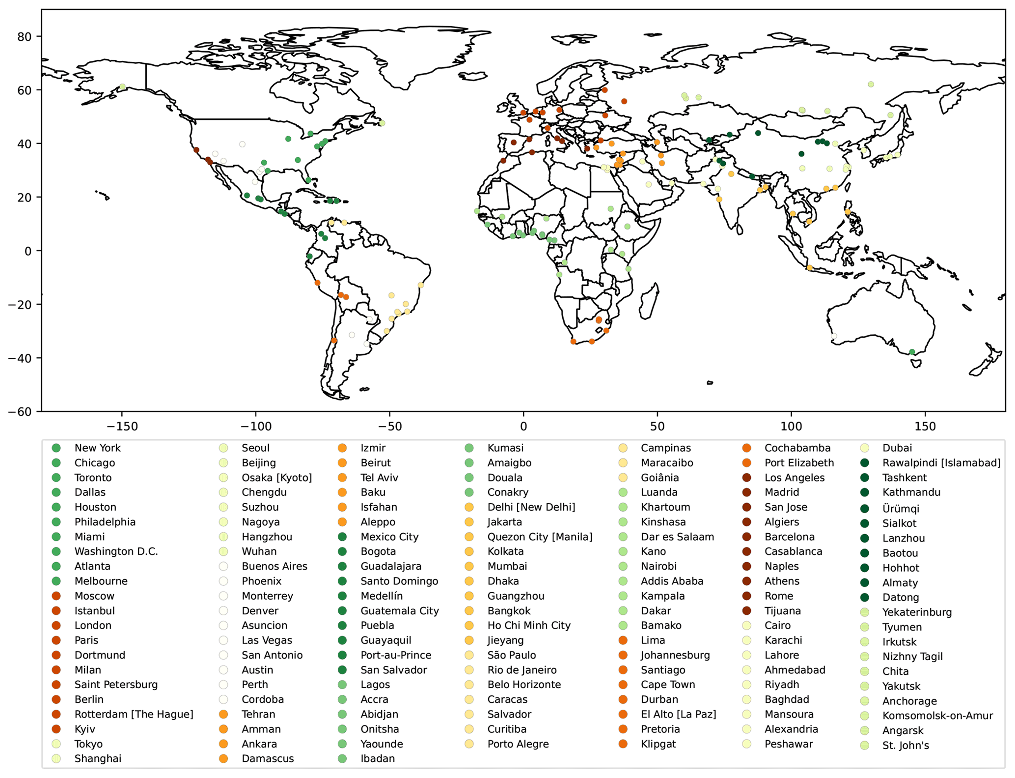
Figure C1Spatial distribution of the 10 most populated functional urban areas per urban ecoregion. Note that ER colours are adopted from Schneider et al. (2010).
Corbane et al. (2021) illustrated that there is a strong relationship between the output probabilities of GHS-S2Net and observed building densities, suggesting that the model outputs can be used as a proxy for impervious surface fractions. As an additional benchmark, we evaluate the GHS-S2Net built-up probabilities for the 30 largest (in surface area) European FUAs (Paris, London, Dortmund, Katowice, Oslo, Madrid, Budapest, Warsaw, Berlin, Lyon, Copenhagen, Milan, Frankfurt am Main, Toulouse, Cologne, Hamburg, Vienna, Helsinki, Leeds, Rotterdam, Prague, Belfast, Liège, Rome, Nantes, Gothenburg, Munich, Krakow, Zurich, and Istanbul) against two products from the European Environmental Agency (EEA):
-
the 100 m Copernicus high-resolution imperviousness density (IMD) layer for 2018 (European Environment Agency, 2018a), a thematic product that indicates the total sealing density (λT), ranging from 0 % to 100 %, and
-
the 100 m share of built-up (SBU) layer for 2018 (European Environment Agency, 2018b), an aggregated version of the 10 m impervious built-up map that indicates the building surface fraction (λB), ranging from 0 % to 100 %.
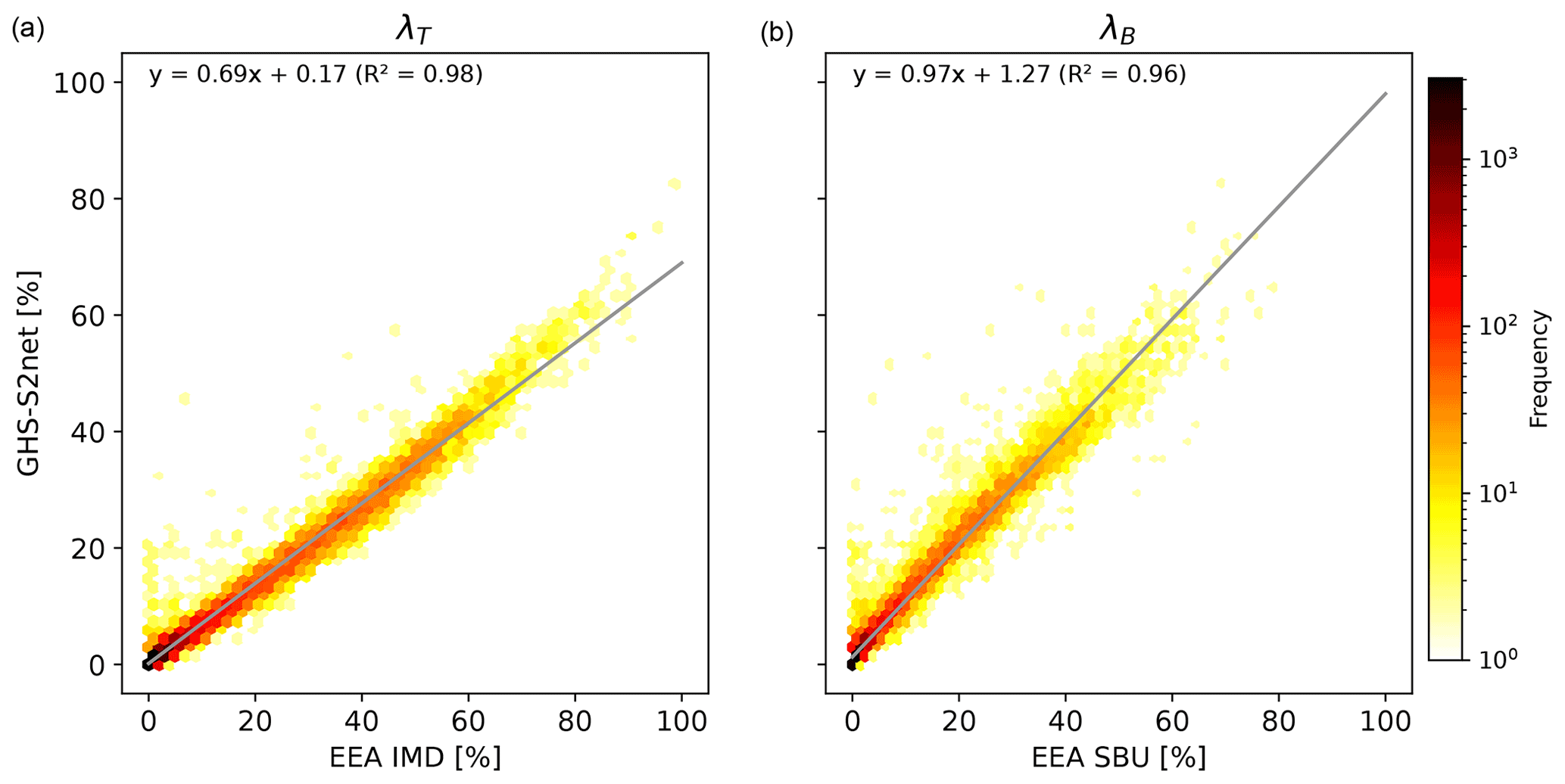
Figure D1Hexbin illustration of the EEA imperviousness density (IMD, reflecting λT) and share of built-up (SBU, reflecting λB) against GHS-S2Net built-up probabilities for the European functional urban area (FUA) of Dortmund (Germany). Linear regression equations and R2 values are provided for both λT (a) and λB (b). The logarithmic colour bar represents the number of pixels in each imperviousness bin.
In line with Bechtel et al. (2019a), all data layers are resampled to a common 1 km grid. Afterwards, EEA's IMD (λT) and SBU (λB) land-only pixels are regressed against the GHS-S2Net built-up probabilities for all 30 European FUAs (see Fig. D1 as an illustration), and the corresponding coefficients of determination (R2) and slopes are reported for λT and λB separately (Fig. D2). Most R2 values exceed 0.9 for both λT and λB, confirming that GHS-S2net is able to explain most of the observed EEA impervious surface fractions. On average, the slopes of the regression between the built-up probabilities of GHS-S2Net and EEA's IMD and SBU products are 0.6 and 0.7 respectively. These results confirm the findings of Corbane et al. (2021) that the GHS-S2net built-up probabilities can serve as a proxy for λB.
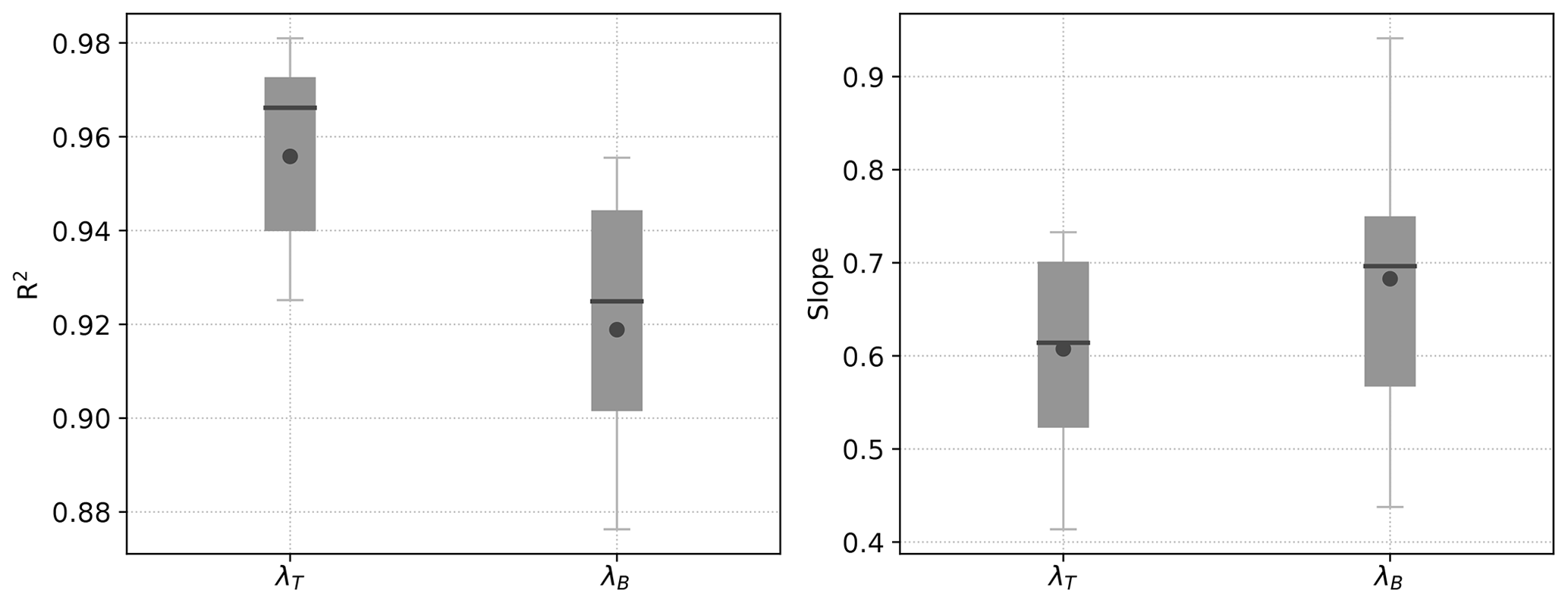
Figure D2Distribution of R2 values and slopes for the regressions between GHS-S2Net and EEA's IMD (λT) and SBU (λB) datasets for the 30 selected European FUA boundaries. Grey boxes and whiskers span the 25th–75th and 5th–95th percentiles respectively. The means and medians are indicated by the black dots and lines respectively.
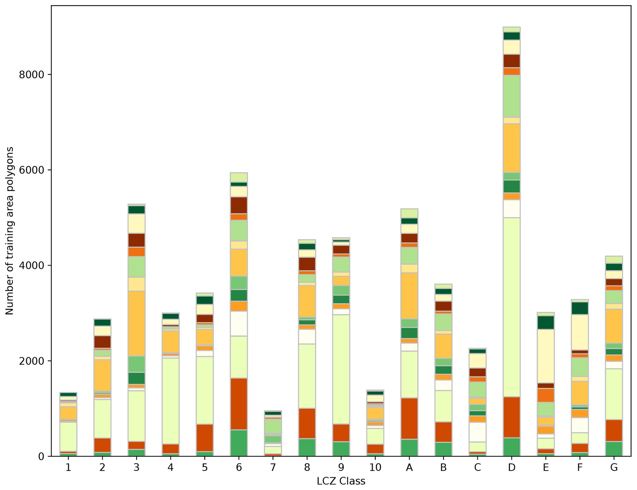
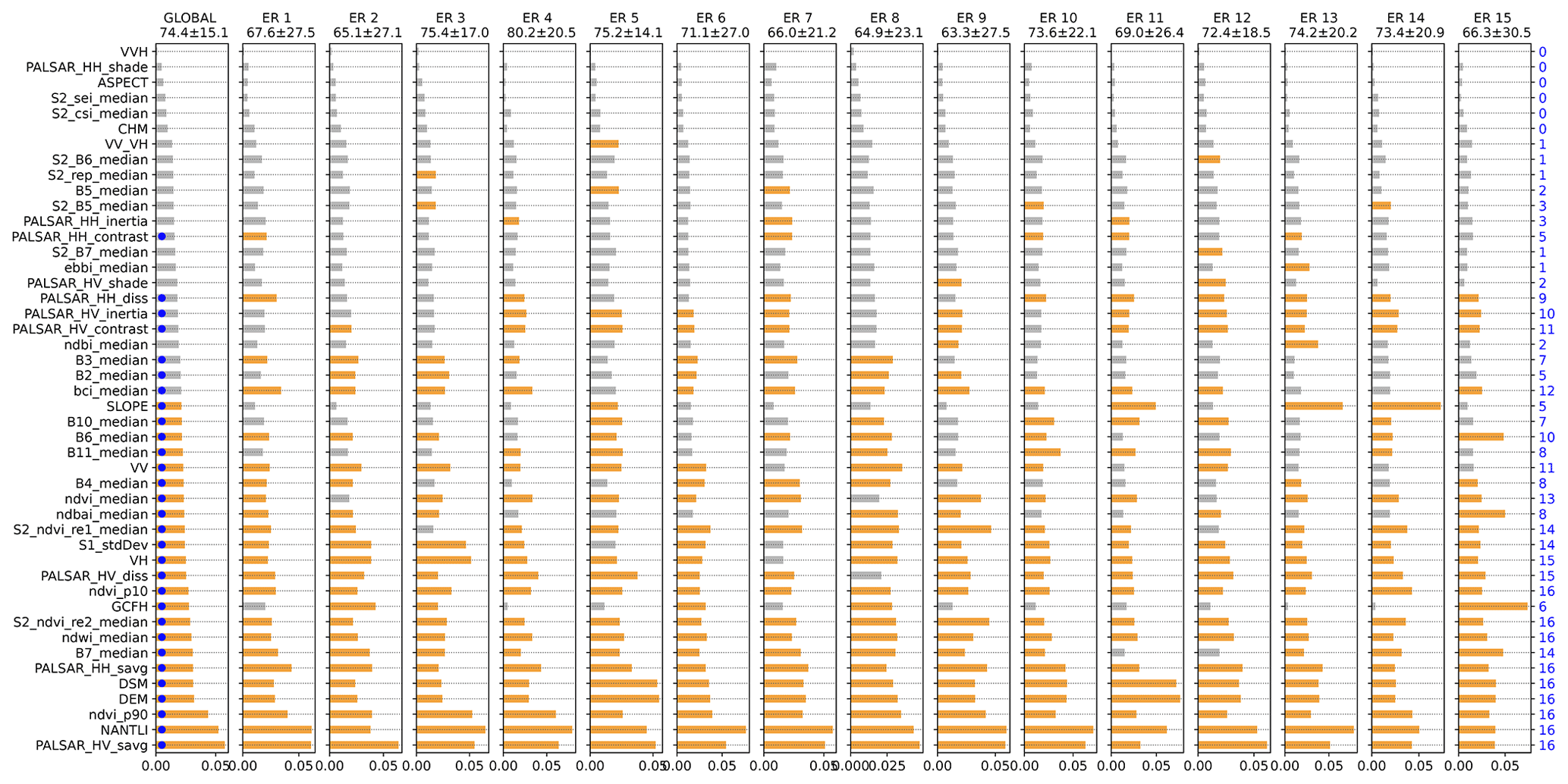
Figure F1Feature importance ranking for the globe and per urban ER. Bars in bright orange depict the input features (per spatial unit) that belong to the top 50 % of the most important variables. Numbers on top depict the overall accuracy ± the standard deviation (%). Blue numbers on the right-hand side describe how often an input feature belongs to the top half of the most important features. Features with a value ≥ 5 are used in pathway 2 to create the global LCZ map and are indicated by the blue dot in the global panel on the left. These features are described in more detail in Table F1.
Table F1Final set of input features used in the global LCZ mapping process. The information is structured by a sensor, with the input feature names referring to the abbreviations used in the feature importance ranking shown in Fig. F1.

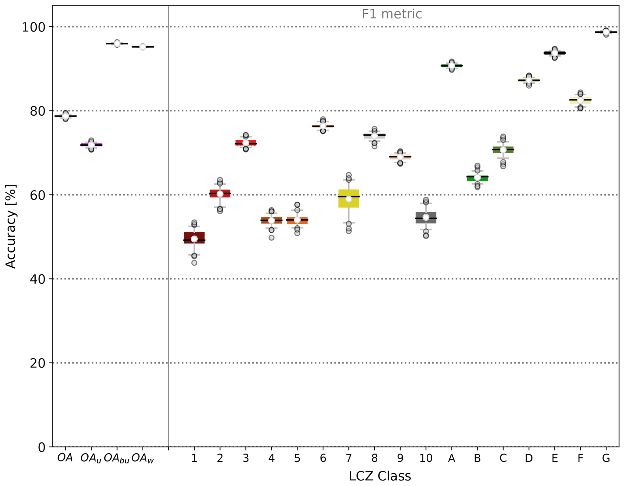
Figure G1Overall and class-wise F1 accuracies for the global random forest LCZ models. Coloured boxes and grey whiskers span the 25th–75th and 5th–95th percentiles respectively. The means and medians are indicated by the white dots and black lines respectively.
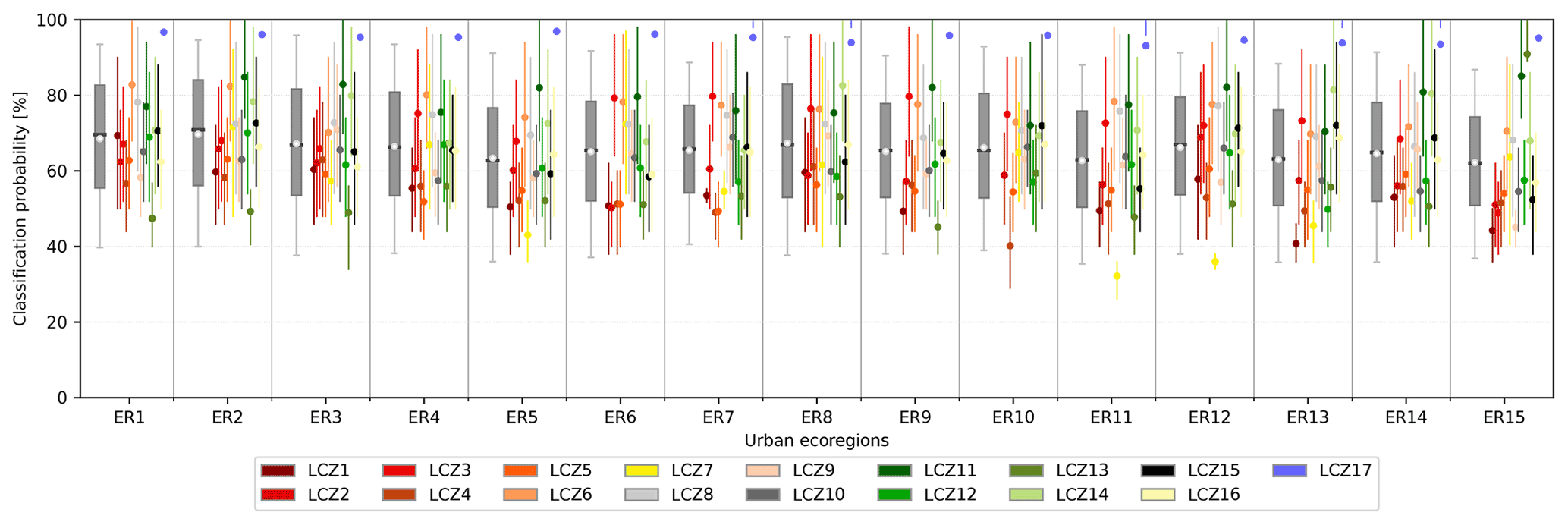
Figure H1Classification probabilities of the mapped LCZ classes, aggregated over all urban centres from GHS-UCDB. The grey boxplots depict the classification probability distribution for all global urban centres, per ER, with boxes and whiskers spanning the 25th–75th and 5th–95th percentiles respectively and means and medians indicated by the white dots and black lines respectively. The vertical lines in the colours of the LCZ classes indicate the 25th–75th percentile range averaged over the urban centres, with LCZ-coloured dots indicating the mean.
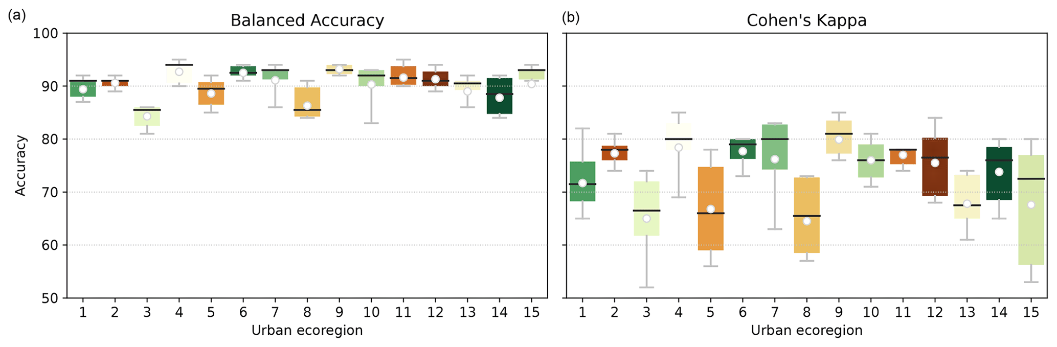
Figure I1Balanced accuracy (a) and Cohen's kappa (b) for the 150 global LCZ FUA regions in terms of built-up land, stratified by urban ecoregion (colours as in Fig. 3). Boxes and grey whiskers span the 25th–75th and 5th–95th percentiles respectively. The means and medians are indicated by the white dots and black lines respectively.
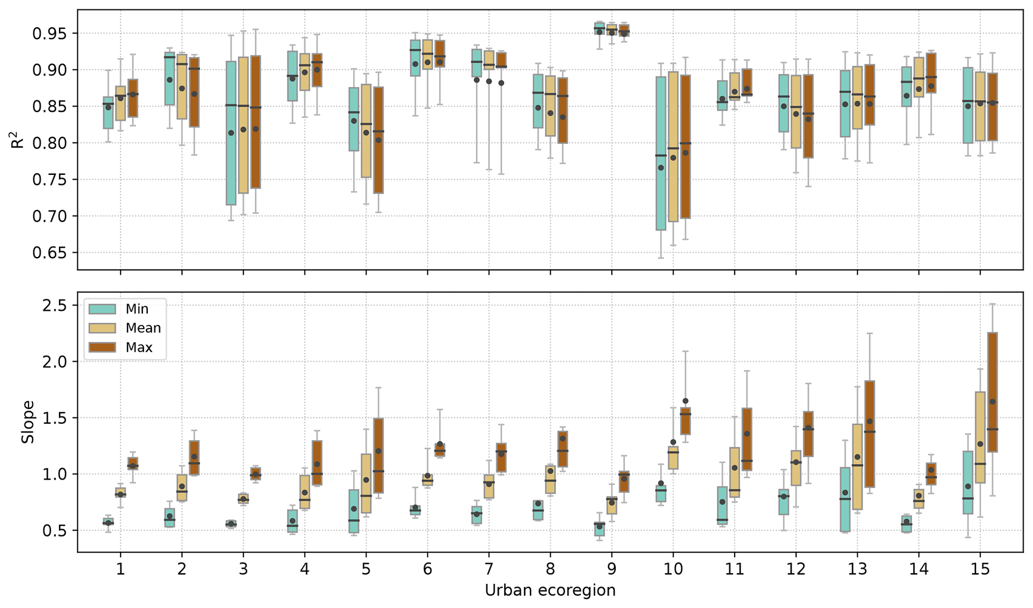
Figure I2Coefficients of determination (R2) and slopes resulting from the regression between the reference dataset for λB and the corresponding universal LCZ-based values from Stewart and Oke (2012), using minimum, mean, and maximum values (colours), for all FUAs stratified per ecoregion. Coloured boxes and grey whiskers span the 25th–75th and 5th–95th percentiles respectively. The means and medians are indicated by the black dots and lines respectively.
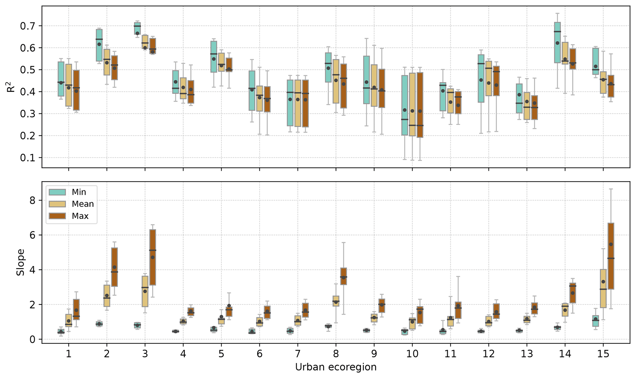

MD designed the research, with feedback from BB and JK. The RUB training area samples were mostly digitized by CM. JK provided technical support with respect to the LCZ Generator database. MD performed all analysis and developed all visualizations. MD wrote the original draft, with contributions from all the other authors.
The contact author has declared that none of the authors has any competing interests.
Publisher's note: Copernicus Publications remains neutral with regard to jurisdictional claims in published maps and institutional affiliations.
We acknowledge all WUDAPT contributors and community members for providing the training areas via the portal or the LCZ Generator, with special thanks to Samira Safaee and Dev Niyogi for providing the large sample of Indian cities. We thank USGS and NASA for the free Landsat data and the Copernicus programme of ESA for the Sentinel data, all acquired and processed via Google's earth engine. We would also like to thank all the research institutes and universities for the creation and provision of open datasets, such as the Copernicus Global Land Cover Layers, the Sentinel-2-based probability of built-up areas, and the anthropogenic heat flux data.
This work was conducted in the context of project ENLIGHT, funded by the German Research Foundation (DFG) under grant no. 437467569. Jasper van Vliet is supported by the Netherlands Organisation for Scientific Research, grant no. VI.vivi.198.008, Guiding human settlements towards sustainable urbanisation.
This paper was edited by David Carlson and reviewed by Jason Ching and two anonymous referees.
Abascal, A., Rothwell, N., Shonowo, A., Thomson, D. R., Elias, P., Elsey, H., Yeboah, G., and Kuffer, M.: “Domains of deprivation framework” for mapping slums, informal settlements, and other deprived areas in LMICs to improve urban planning and policy: A scoping review, Comput. Enviro. Urban, 93, 101770, https://doi.org/10.1016/j.compenvurbsys.2022.101770, 2022. a
Alexander, P., Bechtel, B., Chow, W., Fealy, R., and Mills, G.: Linking urban climate classification with an urban energy and water budget model: Multi-site and multi-seasonal evaluation, Urban Climate, 17, 196–215, https://doi.org/10.1016/j.uclim.2016.08.003, 2016. a
Alexander, P. J., Mills, G., and Fealy, R.: Using LCZ data to run an urban energy balance model, Urban Climate, 13, 14–37, https://doi.org/10.1016/j.uclim.2015.05.001, 2015. a
Aminipouri, M., Knudby, A. J., Krayenhoff, E. S., Zickfeld, K., and Middel, A.: Modelling the impact of increased street tree cover on mean radiant temperature across Vancouver's local climate zones, Urban For. Urban Gree., 39, 9–17, https://doi.org/10.1016/j.ufug.2019.01.016, 2019. a
Assarkhaniki, Z., Sabri, S., and Rajabifard, A.: Using open data to detect the structure and pattern of informal settlements: an outset to support inclusive SDGs' achievement, Big Earth Data, 5, 497–526, https://doi.org/10.1080/20964471.2021.1948178, 2021. a
Bai, X., Dawson, R. J., Ürge-Vorsatz, D., Delgado, G. C., Barau, A. S., Dhakal, S., Dodman, D., Leonardsen, L., Masson-Delmotte, V., Roberts, D., and Schultz, S.: Six research priorities for cities, Nature, 555, 23–25, https://doi.org/10.1038/d41586-018-02409-z, 2018. a, b
Baklanov, A., Grimmond, C., Carlson, D., Terblanche, D., Tang, X., Bouchet, V., Lee, B., Langendijk, G., Kolli, R., and Hovsepyan, A.: From urban meteorology, climate and environment research to integrated city services, Urban Climate, 23, 330–341, https://doi.org/10.1016/j.uclim.2017.05.004, 2018. a
Bande, L., Manandhar, P., Ghazal, R., and Marpu, P.: Characterization of Local Climate Zones Using ENVI-met and Site Data in the City of Al-Ain, UAE, International Journal of Sustainable Development and Planning, 15, 751–760, https://doi.org/10.18280/ijsdp.150517, 2020. a
Barlow, J. F.: Progress in observing and modelling the urban boundary layer, Urban Climate, 10, 216–240, https://doi.org/10.1016/j.uclim.2014.03.011, 2014. a
Bauer, P., Stevens, B., and Hazeleger, W.: A digital twin of Earth for the green transition, Nat. Clim. Change, 11, https://doi.org/10.1038/s41558-021-00986-y, 2021. a
Bechtel, B. and Daneke, C.: Classification of local climate zones based on multiple earth observation data, IEEE J. Sel. Top. Appl., 5, 1191–1202, https://doi.org/10.1109/JSTARS.2012.2189873, 2012. a
Bechtel, B., Alexander, P., Böhner, J., Ching, J., Conrad, O., Feddema, J., Mills, G., See, L., and Stewart, I.: Mapping Local Climate Zones for a Worldwide Database of the Form and Function of Cities, ISPRS International Journal of Geo-Information, 4, 199–219, https://doi.org/10.3390/ijgi4010199, 2015. a, b, c, d, e
Bechtel, B., Demuzere, M., Sismanidis, P., Fenner, D., Brousse, O., Beck, C., Van Coillie, F., Conrad, O., Keramitsoglou, I., Middel, A., Mills, G., Niyogi, D., Otto, M., See, L., and Verdonck, M.-L.: Quality of Crowdsourced Data on Urban Morphology—The Human Influence Experiment (HUMINEX), Urban Science, 1, 15, https://doi.org/10.3390/urbansci1020015, 2017. a, b, c, d
Bechtel, B., Alexander, P. J., Beck, C., Böhner, J., Brousse, O., Ching, J., Demuzere, M., Fonte, C., Gál, T., Hidalgo, J., Hoffmann, P., Middel, A., Mills, G., Ren, C., See, L., Sismanidis, P., Verdonck, M.-L., Xu, G., and Xu, Y.: Generating WUDAPT Level 0 data – Current status of production and evaluation, Urban Climate, 27, 24–45, https://doi.org/10.1016/j.uclim.2018.10.001, 2019a. a
Bechtel, B., Demuzere, M., Mills, G., Zhan, W., Sismanidis, P., Small, C., and Voogt, J.: SUHI analysis using Local Climate Zones – A comparison of 50 cities, Urban Climate, 28, 100451, https://doi.org/10.1016/j.uclim.2019.01.005, 2019b. a
Bechtel, B., Demuzere, M., and Stewart, I. D.: A Weighted Accuracy Measure for Land Cover Mapping: Comment on Johnson et al. Local Climate Zone (LCZ) Map Accuracy Assessments Should Account for Land Cover Physical Characteristics that Affect the Local Thermal Environment, Remote Sens., 12, 1769, https://doi.org/10.3390/rs12111769, 2020. a, b
Beck, C., Straub, A., Breitner, S., Cyrys, J., Philipp, A., Rathmann, J., Schneider, A., Wolf, K., and Jacobeit, J.: Air temperature characteristics of local climate zones in the Augsburg urban area (Bavaria, southern Germany) under varying synoptic conditions, Urban Climate, 25, 152–166, https://doi.org/10.1016/j.uclim.2018.04.007, 2018. a
Benjamin, K., Luo, Z., and Wang, X.: Crowdsourcing Urban Air Temperature Data for Estimating Urban Heat Island and Building Heating/Cooling Load in London, Energies, 14, 5208, https://doi.org/10.3390/en14165208, 2021. a
Bettencourt, L. and West, G.: A unified theory of urban living, Nature, 467, 912–913, https://doi.org/10.1038/467912a, 2010. a
Bettencourt, L. M., Lobo, J., Helbing, D., Kühnert, C., and West, G. B.: Growth, innovation, scaling, and the pace of life in cities, P. Natl. Acad. Sci. USA, 104, 7301–7306, https://doi.org/10.1073/pnas.0610172104, 2007. a
Bettencourt, L. M., Yang, V. C., Lobo, J., Kempes, C. P., Rybski, D., and Hamilton, M. J.: The interpretation of urban scaling analysis in time, J. R. Soc. Interface, 17, 1–9, https://doi.org/10.1098/rsif.2019.0846, 2020. a
Biljecki, F., Chew, L. Z. X., Milojevic-Dupont, N., and Creutzig, F.: Open government geospatial data on buildings for planning sustainable and resilient cities, arXiv [preprint], https://doi.org/10.48550/arXiv.2107.04023, 2021. a
Bokwa, A., Geletič, J., Lehnert, M., Žuvela-Aloise, M., Hollósi, B., Gál, T., Skarbit, N., Dobrovolný, P., Hajto, M. J., Kielar, R., Walawender, J. P., Štastný, P., Holec, J., Ostapowicz, K., Burianová, J., and Garaj, M.: Heat load assessment in Central European cities using an urban climate model and observational monitoring data, Energ. Buildings, 201, 53–69, https://doi.org/10.1016/j.enbuild.2019.07.023, 2019. a
Breiman, L.: Random forests, Mach. Learn., 45, 5–32, https://doi.org/10.1023/A:1010933404324, 2001. a, b
Brousse, O., Martilli, A., Foley, M., Mills, G., and Bechtel, B.: WUDAPT, an efficient land use producing data tool for mesoscale models? Integration of urban LCZ in WRF over Madrid, Urban Climate, 17, 116–134, https://doi.org/10.1016/j.uclim.2016.04.001, 2016. a
Brousse, O., Georganos, S., Demuzere, M., Vanhuysse, S., Wouters, H., Wolff, E., Linard, C., and Lipzig, N. P. V.: Urban Climate Using Local Climate Zones in Sub-Saharan Africa to tackle urban health issues, Urban Climate, 27, 227–242, https://doi.org/10.1016/j.uclim.2018.12.004, 2019. a, b, c
Brousse, O., Georganos, S., Demuzere, M., Dujardin, S., Lennert, M., Linard, C., Snow, R. W., Thiery, W., and van Lipzig, N. P. M.: Can we use local climate zones for predicting malaria prevalence across sub-Saharan African cities?, Environ. Res. Lett., 15, 124051, https://doi.org/10.1088/1748-9326/abc996, 2020a. a, b, c, d, e
Brousse, O., Wouters, H., Demuzere, M., Thiery, W., Van de Walle, J., and Lipzig, N. P. M.: The local climate impact of an African city during clear‐sky conditions – Implications of the recent urbanization in Kampala (Uganda), Int. J. Climatol., 40, 4586–4608, https://doi.org/10.1002/joc.6477, 2020b. a, b
Brousse, O., Simpson, C., Walker, N., Fenner, D., Meier, F., Taylor, J., and Heaviside, C.: Evidence of horizontal urban heat advection in London using six years of data from a citizen weather station network, Environ. Res. Lett., 17, 044041, https://doi.org/10.1088/1748-9326/ac5c0f, 2022. a
Buchhorn, M., Lesiv, M., Tsendbazar, N. E., Herold, M., Bertels, L., and Smets, B.: Copernicus global land cover layers-collection 2, Remote Sens., 12, 1–14, https://doi.org/10.3390/rs12061044, 2020a. a, b
Buchhorn, M., Smets, B., Bertels, L., Roo, B. D., Lesiv, M., Tsendbazar, N.-E., Herold, M., and Fritz, S.: Copernicus Global Land Service: Land Cover 100m: collection 3: epoch 2018: Globe, Zenodo [data set], https://doi.org/10.5281/zenodo.3518038, 2020b. a, b
Chen, C., Bagan, H., Xie, X., La, Y., and Yamagata, Y.: Combination of sentinel-2 and palsar-2 for local climate zone classification: A case study of nanchang, China, Remote Sens., 13, 1–21, https://doi.org/10.3390/rs13101902, 2021a. a, b
Chen, G., Xie, J., Li, W., Li, X., Hay Chung, L. C., Ren, C., and Liu, X.: Future “local climate zon” spatial change simulation in Greater Bay Area under the shared socioeconomic pathways and ecological control line, Build. Environ., 203, 108077, https://doi.org/10.1016/j.buildenv.2021.108077, 2021b. a
Chieppa, J., Bush, A., and Mitra, C.: Using `Local Climate Zones” to detect urban heat island on two small cities in Alabama, Earth Interact., 22, 1–22, https://doi.org/10.1175/EI-D-17-0020.1, 2018. a
Chinchor, N.: MUC-4 evaluation metrics, in: Proceedings of the 4th conference on Message understanding – MUC4 '92, Association for Computational Linguistics, Morristown, NJ, USA, p. 22, https://doi.org/10.3115/1072064.1072067, 1992. a, b
Ching, J., Mills, G., Bechtel, B., See, L., Feddema, J., Wang, X., Ren, C., Brousse, O., Martilli, A., Neophytou, M., Mouzourides, P., Stewart, I., Hanna, A., Ng, E., Foley, M., Alexander, P., Aliaga, D., Niyogi, D., Shreevastava, A., Bhalachandran, P., Masson, V., Hidalgo, J., Fung, J., Andrade, M., Baklanov, A., Dai, W., Milcinski, G., Demuzere, M., Brunsell, N., Pesaresi, M., Miao, S., Mu, Q., Chen, F., and Theeuwes, N.: WUDAPT: An Urban Weather, Climate, and Environmental Modeling Infrastructure for the Anthropocene, B. Am. Meteorol. Soc., 99, 1907–1924, https://doi.org/10.1175/BAMS-D-16-0236.1, 2018. a, b, c, d, e, f, g, h
Ching, J., Aliaga, D., Mills, G., Masson, V., See, L., Neophytou, M., Middel, A., Baklanov, A., Ren, C., Ng, E., Fung, J., Wong, M., Huang, Y., Martilli, A., Brousse, O., Stewart, I., Zhang, X., Shehata, A., Miao, S., Wang, X., Wang, W., Yamagata, Y., Duarte, D., Li, Y., Feddema, J., Bechtel, B., Hidalgo, J., Roustan, Y., Kim, Y., Simon, H., Kropp, T., Bruse, M., Lindberg, F., Grimmond, S., Demuzure, M., Chen, F., Li, C., Gonzales-Cruz, J., Bornstein, B., He, Q., Tzu-Ping, Hanna, A., Erell, E., Tapper, N., Mall, R., and Niyogi, D.: Pathway using WUDAPT's Digital Synthetic City tool towards generating urban canopy parameters for multi-scale urban atmospheric modeling, Urban Climate, 28, 100459, https://doi.org/10.1016/j.uclim.2019.100459, 2019. a, b, c, d
Conners, R. W., Trivedi, M. M., and Harlow, C. A.: Segmentation of a high-resolution urban scene using texture operators (Sunnyvale, California), Comput. Vision Graph., 25, 273–310, https://doi.org/10.1016/0734-189X(84)90197-X, 1984. a
Coops, N. C. and Wulder, M. A.: Breaking the Habit(at), Trend. Ecol. Evol., 34, 585–587, https://doi.org/10.1016/j.tree.2019.04.013, 2019. a
Corbane, C., Pesaresi, M., Politis, P., Syrris, V., Florczyk, A. J., Soille, P., Maffenini, L., Burger, A., Vasilev, V., Rodriguez, D., Sabo, F., Dijkstra, L., and Kemper, T.: Big earth data analytics on Sentinel-1 and Landsat imagery in support to global human settlements mapping, Big Earth Data, 1, 118–144, https://doi.org/10.1080/20964471.2017.1397899, 2017. a
Corbane, C., Pesaresi, M., Kemper, T., Politis, P., Florczyk, A. J., Syrris, V., Melchiorri, M., Sabo, F., and Soille, P.: Automated global delineation of human settlements from 40 years of Landsat satellite data archives, Big Earth Data, 3, 140–169, https://doi.org/10.1080/20964471.2019.1625528, 2019. a
Corbane, C., Politis, P., Kempeneers, P., Simonetti, D., Soille, P., Burger, A., Pesaresi, M., Sabo, F., Syrris, V., and Kemper, T.: A global cloud free pixel- based image composite from Sentinel-2 data, Data in Brief, 31, 105737, https://doi.org/10.1016/j.dib.2020.105737, 2020. a
Corbane, C., Syrris, V., Sabo, F., Politis, P., Melchiorri, M., Pesaresi, M., Soille, P., and Kemper, T.: Convolutional neural networks for global human settlements mapping from Sentinel-2 satellite imagery, Neural Comput. Appl., 33, 6697–6720, https://doi.org/10.1007/s00521-020-05449-7, 2021. a, b, c, d, e, f, g
Costello, A., Abbas, M., Allen, A., Ball, S., Bell, S., Bellamy, R., Friel, S., Groce, N., Johnson, A., Kett, M., Lee, M., Levy, C., Maslin, M., McCoy, D., McGuire, B., Montgomery, H., Napier, D., Pagel, C., Patel, J., de Oliveira, J. A. P., Redclift, N., Rees, H., Rogger, D., Scott, J., Stephenson, J., Twigg, J., Wolff, J., and Patterson, C.: Managing the health effects of climate change, Lancet, 373, 1693–1733, https://doi.org/10.1016/s0140-6736(09)60935-1, 2009. a
Creutzig, F., Baiocchi, G., Bierkandt, R., Pichler, P.-P., and Seto, K. C.: Global typology of urban energy use and potentials for an urbanization mitigation wedge, P. Natl. Acad. Sci. USA, 112, 6283–6288, 201315545, https://doi.org/10.1073/pnas.1315545112, 2015. a
Creutzig, F., Agoston, P., Minx, J. C., Canadell, J. G., Andrew, R. M., Quéré, C. L., Peters, G. P., Sharifi, A., Yamagata, Y., and Dhakal, S.: Urban infrastructure choices structure climate solutions, Nat. Clim. Change, 6, 1054, https://doi.org/10.1038/nclimate3169, 2016. a
Creutzig, F., Lohrey, S., Bai, X., Baklanov, A., Dawson, R., Dhakal, S., Lamb, W. F., McPhearson, T., Minx, J., Munoz, E., and Walsh, B.: Upscaling urban data science for global climate solutions, Global Sustain., 2, 1–25, https://doi.org/10.1017/sus.2018.16, 2019. a
D'Amour, C. B., Reitsma, F., Baiocchi, G., Barthel, S., Güneralp, B., Erb, K. H., Haberl, H., Creutzig, F., and Seto, K. C.: Future urban land expansion and implications for global croplands, P. Natl. Acad. Sci. USA, 114, 8939–8944, https://doi.org/10.1073/pnas.1606036114, 2017. a
Demuzere, M., Orru, K., Heidrich, O., Olazabal, E., Geneletti, D., Orru, H., Bhave, A. G., Mittal, N., Feliu, E., and Faehnle, M.: Mitigating and adapting to climate change: Multi-functional and multi-scale assessment of green urban infrastructure, J. Environ. Manage., 146, 107–115, https://doi.org/10.1016/j.jenvman.2014.07.025, 2014. a
Demuzere, M., Bechtel, B., Middel, A., and Mills, G.: Mapping Europe into local climate zones, PLOS ONE, 14, 1–27, https://doi.org/10.1371/journal.pone.0214474, 2019a. a, b, c, d, e, f
Demuzere, M., Bechtel, B., and Mills, G.: Global transferability of local climate zone models, Urban Climate, 27, 46–63, https://doi.org/10.1016/j.uclim.2018.11.001, 2019b. a, b, c, d, e, f
Demuzere, M., Hankey, S., Mills, G., Zhang, W., Lu, T., and Bechtel, B.: Combining expert and crowd-sourced training data to map urban form and functions for the continental US, Nature Scientific Data, 7, 1–13, https://doi.org/10.1038/s41597-020-00605-z, 2020a. a, b, c, d, e, f, g, h, i, j, k, l, m, n
Demuzere, M., Mihara, T., Redivo, C. P., Feddema, J., and Setton, E.: Multi-temporal LCZ maps for Canadian functional urban areas, OSF Preprints, https://doi.org/10.31219/osf.io/h5tm6, 2020b. a
Demuzere, M., Kittner, J., and Bechtel, B.: LCZ Generator: A Web Application to Create Local Climate Zone Maps, Front. Environ. Sci., 9, 637455, https://doi.org/10.3389/fenvs.2021.637455, 2021b. a, b, c, d, e, f, g, h, i, j, k, l, m
Demuzere, M., Kittner, J., Martilli, A., Mills, G., Moede, C., Stewart, I. D., van Vliet, J., and Bechtel, B.: Global map of Local Climate Zones, Zenodo [data set], https://doi.org/10.5281/zenodo.6364594, 2022a. a, b
Demuzere, M., Kittner, J., Martilli, A., Mills, G., Moede, C., Stewart, I. D., van Vliet, J., and Bechtel, B.: Teaser Local Climate Zone maps extracted from the global map of Local Climate Zones, Zenodo [data set], https://doi.org/10.5281/zenodo.6364705, 2022b. a
Demuzere, M., Argüeso, D., Zonato, A., and Kittner, J.: W2W: A Python package that injects WUDAPT's Local Climate Zone information in WRF (v0.4.1), Zenodo [code], https://doi.org/10.5281/zenodo.7016607, 2022c. a
Di Gregorio, A. and Leonardi, U.: Land cover classification system – user manual software version 3, https://www.fao.org/3/i5428e/i5428e.pdf (last access: 23 August 2022), 2016. a
Dunne, J. P., Horowitz, L. W., Adcroft, A. J., Ginoux, P., Held, I. M., John, J. G., Krasting, J. P., Malyshev, S., Naik, V., Paulot, F., Shevliakova, E., Stock, C. A., Zadeh, N., Balaji, V., Blanton, C., Dunne, K. A., Dupuis, C., Durachta, J., Dussin, R., Gauthier, P. P., Griffies, S. M., Guo, H., Hallberg, R. W., Harrison, M., He, J., Hurlin, W., McHugh, C., Menzel, R., Milly, P. C., Nikonov, S., Paynter, D. J., Ploshay, J., Radhakrishnan, A., Rand, K., Reichl, B. G., Robinson, T., Schwarzkopf, D. M., Sentman, L. T., Underwood, S., Vahlenkamp, H., Winton, M., Wittenberg, A. T., Wyman, B., Zeng, Y., and Zhao, M.: The GFDL Earth System Model Version 4.1 (GFDL-ESM 4.1): Overall Coupled Model Description and Simulation Characteristics, J. Adv. Model. Earth Sy., 12, 1–56, https://doi.org/10.1029/2019MS002015, 2020. a
Eldesoky, A. H., Gil, J., and Pont, M. B.: The suitability of the urban local climate zone classification scheme for surface temperature studies in distinct macroclimate regions, Urban Climate, 37, 100823, https://doi.org/10.1016/j.uclim.2021.100823, 2021. a
ESA: Land Cover CCI Product User Guide Version 2.0, Tech. rep., European Space Agency, http://maps.elie.ucl.ac.be/CCI/viewer/download/ESACCI-LC-Ph2-PUGv2_2.0.pdf (last access: 23 August 2022), 2017. a
Esch, T., Heldens, W., Hirne, A., Keil, M., Marconcini, M., Roth, A., Zeidler, J., Dech, S., and Strano, E.: Breaking new ground in mapping human settlements from space – The Global Urban Footprint, ISPRS J. Photogramm., 134, 30–42, https://doi.org/10.1016/j.isprsjprs.2017.10.012, 2017. a
Esch, T., Brzoska, E., Dech, S., Leutner, B., Palacios-Lopez, D., Metz-Marconcini, A., Marconcini, M., Roth, A., and Zeidler, J.: World Settlement Footprint 3D – A first three-dimensional survey of the global building stock, Remote Sens. Environ., 270, 112877, https://doi.org/10.1016/j.rse.2021.112877, 2022. a
European Environment Agency: Copernicus Land Monitoring Service – High Resolution Layers – Imperviousness Density, https://land.copernicus.eu/pan-european/high-resolution-layers/imperviousness/status-maps/imperviousness-density-2018 (last access: 22 August 2022), 2018a. a, b, c
European Environment Agency: Copernicus Land Monitoring Service – High Resolution Layers – Impervious Built-up, https://land.copernicus.eu/pan-european/high-resolution-layers/imperviousness/status-maps/impervious-built-up-2018 (last access: 22 August 2022), 2018b. a, b
Fenner, D., Meier, F., Bechtel, B., Otto, M., and Scherer, D.: Intra and inter “local climate zone” variability of air temperature as observed by crowdsourced citizen weather stations in Berlin, Germany, Meteorol. Z., 26, 525–547, https://doi.org/10.1127/metz/2017/0861, 2017. a
Fenner, D., Bechtel, B., Demuzere, M., Kittner, J., and Meier, F.: CrowdQC+ – A Quality-Control for Crowdsourced Air-Temperature Observations Enabling World-Wide Urban Climate Applications, Front. Environ. Sci., 9, 1–21, https://doi.org/10.3389/fenvs.2021.720747, 2021. a
Florczyk, A., Melchiorri, M., Corban, C., Schiavina, M., Maffenini, L., Pesaresi, M., Politis, P., Sabo, F., Carneiro Freire, S., Ehrlich, D., Kemper, T., Tommasi, P., Airaghi, D., and Zanchetta, L.: Description of the GHS Urban Centre Database 2015, public release 2019, version 1.0, Publications Office, https://doi.org/10.2760/037310, 2019. a, b
Forget, Y., Shimoni, M., and Gilbert, M.: Complementarity Between Sentinel-1 and Landsat 8 Imagery for Built-Up Mapping in Sub-Saharan Africa, Preprints 2018, 2018100695, https://doi.org/10.20944/preprints201810.0695.v1, 2018. a
Fuhrer, O., Chadha, T., Hoefler, T., Kwasniewski, G., Lapillonne, X., Leutwyler, D., Lüthi, D., Osuna, C., Schär, C., Schulthess, T. C., and Vogt, H.: Near-global climate simulation at 1 km resolution: establishing a performance baseline on 4888 GPUs with COSMO 5.0, Geosci. Model Dev., 11, 1665–1681, https://doi.org/10.5194/gmd-11-1665-2018, 2018. a
Gál, T., Mahó, S. I., Skarbit, N., and Unger, J.: Numerical modelling for analysis of the effect of different urban green spaces on urban heat load patterns in the present and in the future, Comput. Environ. Urban, 87, 101600, https://doi.org/10.1016/j.compenvurbsys.2021.101600, 2021. a
Georgescu, M., Chow, W. T. L., Wang, Z. H., Brazel, A., Trapido-Lurie, B., Roth, M., and Benson-Lira, V.: Prioritizing urban sustainability solutions: coordinated approaches must incorporate scale-dependent built environment induced effects, Environ. Res. Lett., 10, 061001, https://doi.org/10.1088/1748-9326/10/6/061001, 2015. a
Gilabert, J., Deluca, A., Lauwaet, D., Ballester, J., Corbera, J., and Llasat, M. C.: Assessing heat exposure to extreme temperatures in urban areas using the Local Climate Zone classification, Nat. Hazards Earth Syst. Sci., 21, 375–391, https://doi.org/10.5194/nhess-21-375-2021, 2021. a
Gong, P., Li, X., Wang, J., Bai, Y., Chen, B., Hu, T., Liu, X., Xu, B., Yang, J., Zhang, W., and Zhou, Y.: Annual maps of global artificial impervious area (GAIA) between 1985 and 2018, Remote Sens. Environ., 236, 111510, https://doi.org/10.1016/j.rse.2019.111510, 2020. a, b
Gorelick, N., Hancher, M., Dixon, M., Ilyushchenko, S., Thau, D., and Moore, R.: Google Earth Engine: Planetary-scale geospatial analysis for everyone, Remote Sens. Environ., 202, 18–27, https://doi.org/10.1016/j.rse.2017.06.031, 2017. a
Grimm, N. B., Faeth, S. H., Golubiewski, N. E., Redman, C. L., Wu, J., Bai, X., and Briggs, J. M.: Global change and the ecology of cities, Science, 319, 756–760, https://doi.org/10.1126/science.1150195, 2008. a
Grimmond, S., Bouchet, V., Molina, L. T., Baklanov, A., Tan, J., Schlünzen, K. H., Mills, G., Golding, B., Masson, V., Ren, C., Voogt, J., Miao, S., Lean, H., Heusinkveld, B., Hovespyan, A., Teruggi, G., Parrish, P., and Joe, P.: Integrated urban hydrometeorological, climate and environmental services: Concept, methodology and key messages, Urban Climate, 33, 100623, https://doi.org/10.1016/j.uclim.2020.100623, 2020. a
Güneralp, B., Zhou, Y., Ürge-Vorsatz, D., Gupta, M., Yu, S., Patel, P. L., Fragkias, M., Li, X., and Seto, K. C.: Global scenarios of urban density and its impacts on building energy use through 2050, P. Natl. Acad. Sci. USA, 114, 8945–8950, https://doi.org/10.1073/pnas.1606035114, 2017. a
Gutowski, W. J., Ullrich, P. A., Hall, A., Leung, L. R., O'Brien, T. A., Patricola, C. M., Arritt, R. W., Bukovsky, M. S., Calvin, K. V., Feng, Z., Jones, A. D., Kooperman, G. J., Monier, E., Pritchard, M. S., Pryor, S. C., Qian, Y., Rhoades, A. M., Roberts, A. F., Sakaguchi, K., Urban, N., and Zarzycki, C.: The Ongoing Need for High-Resolution Regional Climate Models: Process Understanding and Stakeholder Information, B. Am. Meteorol. Soc., 101, E664–E683, https://doi.org/10.1175/BAMS-D-19-0113.1, 2020. a
Hammerberg, K., Brousse, O., Martilli, A., and Mahdavi, A.: Implications of employing detailed urban canopy parameters for mesoscale climate modelling: a comparison between WUDAPT and GIS databases over Vienna, Austria, Int. J. Climatol., 38, e1241–e1257, https://doi.org/10.1002/joc.5447, 2018. a
Haralick, R. M., Dinstein, I., and Shanmugam, K.: Textural Features for Image Classification, IEEE T. Syst. Man Cyb., SMC-3, 610–621, https://doi.org/10.1109/TSMC.1973.4309314, 1973. a
Hay Chung, L. C., Xie, J., and Ren, C.: Improved machine-learning mapping of local climate zones in metropolitan areas using composite Earth observation data in Google Earth Engine, Build. Environ., 199, 107879, https://doi.org/10.1016/j.buildenv.2021.107879, 2021. a, b, c
Hertwig, D., Ng, M., Grimmond, S., Vidale, P. L., and McGuire, P. C.: High‐resolution global climate simulations: Representation of cities, Int. J. Climatol., 41, 3266–3285, https://doi.org/10.1002/joc.7018, 2021. a, b
Hidalgo, J., Lemonsu, A., and Masson, V.: Between progress and obstacles in urban climate interdisciplinary studies and knowledge transfer to society, Ann. NY Acad. Sci., 1436, 5–18, https://doi.org/10.1111/nyas.13986, 2018. a
Hirsch, A. L., Evans, J. P., Thomas, C., Conroy, B., Hart, M. A., Lipson, M., and Ertler, W.: Resolving the influence of local flows on urban heat amplification during heatwaves, Environ. Res. Lett., 16, 064066, https://doi.org/10.1088/1748-9326/ac0377, 2021. a
Hu, J., Ghamisi, P., and Zhu, X.: Feature Extraction and Selection of Sentinel-1 Dual-Pol Data for Global-Scale Local Climate Zone Classification, ISPRS Int. Geo-Inf., 7, 379, https://doi.org/10.3390/ijgi7090379, 2018. a
IPCC: Climate Change 2022: Impacts, Adaptation, and Vulnerability, Contribution of Working Group II to the Sixth Assessment Report of the Intergovernmental Panel on Climate Change, edited by: Pörtner, H.-O., Roberts, D. C., Tignor, M., Poloczanska, E. S., Mintenbeck, K., Alegría, A., Craig, M., Langsdorf, S., Löschke, S., Möller, V., Okem, A., and Rama, B., Cambridge University Press, in Press, 2022. a
Jiang, S., Huang, F., Zhan, W., Bechtel, B., Liu, Z., Demuzere, M., Huang, Y., Xu, Y., Xia, W., Quan, J., Hong, F., Jiang, L., Lai, J., Wang, C., Kong, F., Du, H., Miao, S., Chen, Y., Zhang, X., Planning, R., and Development, U.: Mapping Local Climate Zones : A Bibliometric Meta- Analysis and Systematic Review, OSF preprints, 1–106, https://doi.org/10.31219/osf.io/c2bez, 2021. a, b
Jung, M., Dahal, P. R., Butchart, S. H., Donald, P. F., De Lamo, X., Lesiv, M., Kapos, V., Rondinini, C., and Visconti, P.: A global map of terrestrial habitat types, Sci. Data, 7, 1–8, https://doi.org/10.1038/s41597-020-00599-8, 2020. a
Kabano, P., Lindley, S., and Harris, A.: Evidence of urban heat island impacts on the vegetation growing season length in a tropical city, Landscape Urban Plan., 206, 103989, https://doi.org/10.1016/j.landurbplan.2020.103989, 2021. a
Kamath, H. G., Singh, M., Magruder, L. A., Yang, Z.-l., and Niyogi, D.: GLOBUS: GLObal Building heights for Urban Studies, ArXiv [preprint], https://doi.org/10.48550/arXiv.2205.12224, 2022. a
Karsisto, P., Fortelius, C., Demuzere, M., Grimmond, C. S. B., Oleson, K. W., Kouznetsov, R., Masson, V., and Järvi, L.: Seasonal surface urban energy balance and wintertime stability simulated using three land-surface models in the high-latitude city Helsinki, Q. J. Roy. Meteor. Soc., 142, 401–417, https://doi.org/10.1002/qj.2659, 2016. a
Kotharkar, R., Ghosh, A., Kapoor, S., and Reddy, D. G. K.: Approach to local climate zone based energy consumption assessment in an Indian city, Energ. Buildings, 259, 111835, https://doi.org/10.1016/j.enbuild.2022.111835, 2022. a
Kuffer, M., Thomson, D. R., Boo, G., Mahabir, R., Grippa, T., Vanhuysse, S., Engstrom, R., Ndugwa, R., Makau, J., Darin, E., de Albuquerque, J. P., and Kabaria, C.: The role of earth observation in an integrated deprived area mapping “system” for low-to-middle income countries, Remote Sensing, 12, 982, https://doi.org/10.3390/rs12060982, 2020. a
Lai, D., Liu, W., Gan, T., Liu, K., and Chen, Q.: A review of mitigating strategies to improve the thermal environment and thermal comfort in urban outdoor spaces, Sci. Total Environ., 661, 337–353, https://doi.org/10.1016/j.scitotenv.2019.01.062, 2019. a
Leconte, F., Bouyer, J., and Claverie, R.: Nocturnal cooling in Local Climate Zone: Statistical approach using mobile measurements, Urban Climate, 33, 100629, https://doi.org/10.1016/j.uclim.2020.100629, 2020. a
Lehnert, M., Savić, S., Milošević, D., Dunjić, J., and Geletič, J.: Mapping Local Climate Zones and Their Applications in European Urban Environments: A Systematic Literature Review and Future Development Trends, ISPRS Int. Geo-Inf., 10, 260, https://doi.org/10.3390/ijgi10040260, 2021. a
Li, M., Koks, E., Taubenböck, H., and van Vliet, J.: Continental-scale mapping and analysis of 3D building structure, Remote Sens. Environ., 245, 111859, https://doi.org/10.1016/j.rse.2020.111859, 2020. a, b
Li, X., Gong, P., Zhou, Y., Wang, J., Bai, Y., Chen, B., Hu, T., Xiao, Y., Xu, B., Yang, J., Liu, X., Cai, W., Huang, H., Wu, T., Wang, X., Lin, P., Li, X., Chen, J., He, C., Li, X., Yu, L., Clinton, N., and Zhu, Z.: Mapping global urban boundaries from the global artificial impervious area (GAIA) data, Environ. Res. Lett., 15, 094044, https://doi.org/10.1088/1748-9326/ab9be3, 2020. a
Lindberg, F., Grimmond, C., Gabey, A., Huang, B., Kent, C. W., Sun, T., Theeuwes, N. E., Järvi, L., Ward, H. C., Capel-Timms, I., Chang, Y., Jonsson, P., Krave, N., Liu, D., Meyer, D., Olofson, K. F. G., Tan, J., Wästberg, D., Xue, L., and Zhang, Z.: Urban Multi-scale Environmental Predictor (UMEP): An integrated tool for city-based climate services, Environ. Model. Softw., 99, 70–87, https://doi.org/10.1016/j.envsoft.2017.09.020, 2018. a
Liu, S., Qi, Z., Li, X., and Yeh, A. G.-O.: Integration of Convolutional Neural Networks and Object-Based Post-Classification Refinement for Land Use and Land Cover Mapping with Optical and SAR Data, Remote Sensing, 11, 690, https://doi.org/10.3390/rs11060690, 2019. a
Lu, T., Marshall, J. D., Zhang, W., Hystad, P., Kim, S.-Y., Bechle, M. J., Demuzere, M., and Hankey, S.: National Empirical Models of Air Pollution Using Microscale Measures of the Urban Environment, Environ. Sci. Technol., 55, 15519–15530, https://doi.org/10.1021/acs.est.1c04047, 2021. a
Lu, Y., Yang, J., and Ma, S.: Dynamic Changes of Local Climate Zones in the Guangdong–Hong Kong–Macao Greater Bay Area and Their Spatio-Temporal Impacts on the Surface Urban Heat Island Effect between 2005 and 2015, Sustainability, 13, 6374, https://doi.org/10.3390/su13116374, 2021. a
Lyu, T., Buccolieri, R., and Gao, Z.: A numerical study on the correlation between sky view factor and summer microclimate of local climate zones, Atmosphere, 10, 438, https://doi.org/10.3390/atmos10080438, 2019. a
MacKenzie, A. R., Whyatt, J. D., Barnes, M. J., Davies, G., and Hewitt, C. N.: Urban form strongly mediates the allometric scaling of airshed pollution concentrations, Environ. Res. Lett., 14, 124078, https://doi.org/10.1088/1748-9326/ab50e3, 2019. a
Maharoof, N., Emmanuel, R., and Thomson, C.: Compatibility of local climate zone parameters for climate sensitive street design: Influence of openness and surface properties on local climate, Urban Climate, 33, 100642, https://doi.org/10.1016/j.uclim.2020.100642, 2020. a
Manoli, G., Fatichi, S., Schläpfer, M., Yu, K., Crowther, T. W., Meili, N., Burlando, P., Katul, G. G., and Bou-Zeid, E.: Magnitude of urban heat islands largely explained by climate and population, Nature, 573, 55–60, https://doi.org/10.1038/s41586-019-1512-9, 2019. a, b
Marconcini, M., Metz-Marconcini, A., Üreyen, S., Palacios-Lopez, D., Hanke, W., Bachofer, F., Zeidler, J., Esch, T., and Strano, E.: World Settlement Footprint (WSF) 2015 – Percent Settlement Area – 100m, Figshare [data set], https://doi.org/10.6084/m9.figshare.10048475.v1, 2020. a, b, c, d, e
Martilli, A.: An idealized study of city structure, urban climate, energy consumption, and air quality, Urban Climate, 10, 430–446, https://doi.org/10.1016/j.uclim.2014.03.003, 2014. a
Martilli, A., Roth, M., Winston, T. L., Demuzere, M., Lipson, M., Krayenhoff, S., Sailor, D., Nazarian, N., Voogt, J., Wouters, H., Middel, A., Stewart, I. D., Bechtel, B., Christen, A., and Hart, M.: Summer average urban-rural surface temperature differences do not indicate the need for urban heat reduction, OSF preprints, https://doi.org/10.31219/osf.io/8gnbf, 2020. a, b
Masson, V., Heldens, W., Bocher, E., Bonhomme, M., Bucher, B., Burmeister, C., de Munck, C., Esch, T., Hidalgo, J., Kanani-Sühring, F., Kwok, Y. T., Lemonsu, A., Lévy, J. P., Maronga, B., Pavlik, D., Petit, G., See, L., Schoetter, R., Tornay, N., Votsis, A., and Zeidler, J.: City-descriptive input data for urban climate models: Model requirements, data sources and challenges, Urban Climate, 31, 100536, https://doi.org/10.1016/j.uclim.2019.100536, 2020. a
Matsaba, E. O., Langer, I., Adimo, A. O., Mukundi, J. B., and Wesonga, J. M.: Spatio-Temporal Variability of Simulated 2 m Air Temperature for Nairobi City, Kenya, Current Urban Studies, 8, 205–221, https://doi.org/10.4236/cus.2020.82011, 2020. a
McDonough, L. K., Santos, I. R., Andersen, M. S., O'Carroll, D. M., Rutlidge, H., Meredith, K., Oudone, P., Bridgeman, J., Gooddy, D. C., Sorensen, J. P., Lapworth, D. J., MacDonald, A. M., Ward, J., and Baker, A.: Changes in global groundwater organic carbon driven by climate change and urbanization, Nat. Commun., 11, 1–10, https://doi.org/10.1038/s41467-020-14946-1, 2020. a, b
Middel, A., Häb, K., Brazel, A. J., Martin, C. a., and Guhathakurta, S.: Impact of urban form and design on mid-afternoon microclimate in Phoenix Local Climate Zones, Landscape Urban Plan., 122, 16–28, https://doi.org/10.1016/j.landurbplan.2013.11.004, 2014. a
Mills, S., Weiss, S., and Liang, C.: VIIRS day/night band (DNB) stray light characterization and correction, in: Earth Observing Systems XVIII, edited by: Butler, J. J., Xiong, X. J., and Gu, X., International Society for Optics and Photonics, SPIE, 8866, 549–566, https://doi.org/10.1117/12.2023107, 2013. a
Milošević, D., Savić, S., Kresoja, M., Lužanin, Z., Šećerov, I., Arsenović, D., Dunjić, J., and Matzarakis, A.: Analysis of air temperature dynamics in the “local climate zones” of Novi Sad (Serbia) based on long-term database from an urban meteorological network, Int. J. Biometeorol., 66, 371–384, https://doi.org/10.1007/s00484-020-02058-w, 2021. a
Molnár, G., Gyöngyösi, A. Z., and Gál, T.: Integration of an LCZ-based classification into WRF to assess the intra-urban temperature pattern under a heatwave period in Szeged, Hungary, Theor. Appl. Climatol., 138, 1139–1158, https://doi.org/10.1007/s00704-019-02881-1, 2019. a
Moradi, M., Krayenhoff, E. S., and Aliabadi, A. A.: A comprehensive indoor–outdoor urban climate model with hydrology: The Vertical City Weather Generator (VCWG v2.0.0), Build. Environ., 207, 108406, https://doi.org/10.1016/j.buildenv.2021.108406, 2022. a
Mu, Q., Miao, S., Wang, Y., Li, Y., He, X., and Yan, C.: Evaluation of employing local climate zone classification for mesoscale modelling over Beijing metropolitan area, Meteorol. Atmos. Phys., 132, 315–326, https://doi.org/10.1007/s00703-019-00692-7, 2020. a
Nagendra, H., Bai, X., Brondizio, E. S., and Lwasa, S.: The urban south and the predicament of global sustainability, Nature Sustainability, 1, 341–349, https://doi.org/10.1038/s41893-018-0101-5, 2018. a
Oke, T. R., Mills, G., Christen, A., and Voogt, J. A.: Urban Climates, Cambridge University Press, Cambridge, https://doi.org/10.1017/9781139016476, 2017. a, b, c
Oleson, K. W. and Feddema, J.: Parameterization and Surface Data Improvements and New Capabilities for the Community Land Model Urban (CLMU), J. Adv. Model. Earth Sy., 12, 1–30, https://doi.org/10.1029/2018ms001586, 2020. a, b
Owusu, M., Kuffer, M., Belgiu, M., Grippa, T., Lennert, M., Georganos, S., and Vanhuysse, S.: Towards user-driven earth observation-based slum mapping, Comput. Environ. Urban, 89, 101681, https://doi.org/10.1016/j.compenvurbsys.2021.101681, 2021. a
Pan, Z.: WUDAPT Level 0 training data for HUAICHU (China, People's Republic of), LCZ Generator, submitted, https://lcz-generator.rub.de/factsheets/f81f240993b6ca50180232c878755c18736e308a/f81f240993b6ca50180232c878755c18736e308a_factsheet.html (last access: 22 August 2022), 2021. a
Patel, P., Karmakar, S., Ghosh, S., and Niyogi, D.: Improved simulation of very heavy rainfall events by incorporating WUDAPT urban land use/land cover in WRF, Urban Climate, 32, 100616, https://doi.org/10.1016/j.uclim.2020.100616, 2020. a
Patel, P., Jamshidi, S., Nadimpalli, R., Aliaga, D. G., Mills, G., Chen, F., Demuzere, M., and Niyogi, D.: Modeling Large‐Scale Heatwave by Incorporating Enhanced Urban Representation, J. Geophys. Res.-Atmos., 127, 1–33, https://doi.org/10.1029/2021JD035316, 2022. a, b
Patella, V., Florio, G., Magliacane, D., Giuliano, A., Crivellaro, M. A., Bartolomeo, D., Genovese, A., Palmieri, M., Postiglione, A., Ridolo, E., Scaletti, C., Ventura, M. T., and Zollo, A.: Urban air pollution and climate change: “The Decalogue: Allergy Safe Tree” for allergic and respiratory diseases care, Clinical and Molecular Allergy, 16, 20, https://doi.org/10.1186/s12948-018-0098-3, 2018. a
Pedregosa, F., Varoquaux, G., Gramfort, A., Michel, V., Thirion, B., Grisel, O., Blondel, M., Prettenhofer, P., Weiss, R., Dubourg, V., Vanderplas, J., Passos, A., Cournapeau, D., Brucher, M., Perrot, M., and Duchesnay, E.: Scikit-learn: Machine Learning in {P}ython, J. Mach. Learn. Res., 12, 2825–2830, 2011. a, b
Pellegatti Franco, D. M., Andrade, M. d. F., Ynoue, R. Y., and Ching, J.: Effect of Local Climate Zone (LCZ) classification on ozone chemical transport model simulations in Sao Paulo, Brazil, Urban Climate, 27, 293–313, https://doi.org/10.1016/j.uclim.2018.12.007, 2019. a
Perera, N. and Emmanuel, R.: A “Local Climate Zone” based approach to urban planning in Colombo, Sri Lanka, Urban Climate, 23, 188–203, https://doi.org/10.1016/j.uclim.2016.11.006, 2018. a
Potapov, P., Li, X., Hernandez-Serna, A., Tyukavina, A., Hansen, M. C., Kommareddy, A., Pickens, A., Turubanova, S., Tang, H., Silva, C. E., Armston, J., Dubayah, R., Blair, J. B., and Hofton, M.: Mapping global forest canopy height through integration of GEDI and Landsat data, Remote Sens. Environ., 253, 112165, https://doi.org/10.1016/j.rse.2020.112165, 2021. a
Potgieter, J., Nazarian, N., Lipson, M. J., Hart, M. A., Ulpiani, G., Morrison, W., and Benjamin, K.: Combining High-Resolution Land Use Data With Crowdsourced Air Temperature to Investigate Intra-Urban Microclimate, Front. Environ. Sci., 9, 1–19, https://doi.org/10.3389/fenvs.2021.720323, 2021. a
Quah, A. K. and Roth, M.: Diurnal and weekly variation of anthropogenic heat emissions in a tropical city, Singapore, Atmos. Environ., 46, 92–103, https://doi.org/10.1016/j.atmosenv.2011.10.015, 2012. a
Raven, J., Stone, B., Mills, G., Towers, J., Katzschner, L., Leone, M. F., Gaborit, P., Georgescu, M., Hariri, M., Lee, J., LeJava, J., Sharifi, A., Visconti, C., and Rudd, A.: Urban Planning and Urban Design, in: Climate Change and Cities, Cambridge University Press, 139–172, https://doi.org/10.1017/9781316563878.012, 2018. a
Reba, M. and Seto, K. C.: A systematic review and assessment of algorithms to detect, characterize, and monitor urban land change, Remote Sens. Environ., 242, 111739, https://doi.org/10.1016/j.rse.2020.111739, 2020. a, b, c
Ribeiro, H. V., Rybski, D., and Kropp, J. P.: Effects of changing population or density on urban carbon dioxide emissions, Nat. Commun., 10, 1–9, https://doi.org/10.1038/s41467-019-11184-y, 2019. a
Rosentreter, J., Hagensieker, R., and Waske, B.: Towards large-scale mapping of local climate zones using multitemporal Sentinel 2 data and convolutional neural networks, Remote Sens. Environ., 237, 111472, https://doi.org/10.1016/j.rse.2019.111472, 2020. a
Rosenzweig, C., Solecki, W., Hammer, S. A., and Mehrotra, S.: Cities lead the way in climate-change action, Nature, 467, 909–911, https://doi.org/10.1038/467909a, 2010. a
Santos, L. G. R., Singh, V. K., Mughal, M. O., Nevat, I., Norford, L. K., and Fonseca, J. A.: Estimating building's anthropogenic heat: a joint local climate zone and land use classification method, eSIM 2021 conference, 12–19, https://doi.org/10.3929/ethz-b-000445814, 2020. a
Sapena, M., Wurm, M., Taubenböck, H., Tuia, D., and Ruiz, L. A.: Estimating quality of life dimensions from urban spatial pattern metrics, Comput. Environ. Urban, 85, 101549, https://doi.org/10.1016/j.compenvurbsys.2020.101549, 2021. a
Schär, C., Fuhrer, O., Arteaga, A., Ban, N., Charpilloz, C., Di Girolamo, S., Hentgen, L., Hoefler, T., Lapillonne, X., Leutwyler, D., Osterried, K., Panosetti, D., Rüdisühli, S., Schlemmer, L., Schulthess, T. C., Sprenger, M., Ubbiali, S., and Wernli, H.: Kilometer-Scale Climate Models: Prospects and Challenges, B. Am. Meteorol. Soc., 101, E567–E587, https://doi.org/10.1175/bams-d-18-0167.1, 2020. a
Schiavina, M., Moreno-Monroy, A., Maffenini, L., and Veneri, P.: GHSL-OECD Functional Urban Areas 2019, https://doi.org/10.2760/67415, 2019. a
Schläpfer, M., Lee, J., and Bettencourt, L. M. A.: Urban Skylines: building heights and shapes as measures of city size, ArXiv [preprint], 1–17, https://doi.org/10.48550/arXiv.1512.00946, 2015. a, b
Schneider, A., Friedl, M. A., and Potere, D.: Mapping global urban areas using MODIS 500-m data: New methods and datasets based on “urban ecoregions”, Remote Sens. Environ., 114, 1733–1746, https://doi.org/10.1016/j.rse.2010.03.003, 2010. a, b, c
Seto, K. C., Güneralp, B., and Hutyra, L. R.: Global forecasts of urban expansion to 2030 and direct impacts on biodiversity and carbon pools., P. Natl. Acad. Sci. USA, 109, 16 083–8, https://doi.org/10.1073/pnas.1211658109, 2012. a
Sharma, R., Hooyberghs, H., Lauwaet, D., and De Ridder, K.: Urban Heat Island and Future Climate Change – Implications for Delhi's Heat, J. Urban Health, 96, 235–251, https://doi.org/10.1007/s11524-018-0322-y, 2019. a
Shimada, M., Itoh, T., Motooka, T., Watanabe, M., Shiraishi, T., Thapa, R., and Lucas, R.: New global forest/non-forest maps from ALOS PALSAR data (2007–2010), Remote Sens. Environm., 155, 13–31, https://doi.org/10.1016/j.rse.2014.04.014, 2014. a
Simard, M., Pinto, N., Fisher, J. B., and Baccini, A.: Mapping forest canopy height globally with spaceborne lidar, J. Geophys. Res., 116, G04021, https://doi.org/10.1029/2011JG001708, 2011. a
Skarbit, N., Stewart, I. D., Unger, J., and Gál, T.: Employing an urban meteorological network to monitor air temperature conditions in the “local climate zones” of Szeged, Hungary, Int. J. Climatol., 37, 582–596, https://doi.org/10.1002/joc.5023, 2017. a
Steeneveld, G.-J., Klompmaker, J. O., Groen, R. J., and Holtslag, A. A.: An urban climate assessment and management tool for combined heat and air quality judgements at neighbourhood scales, Resour. Conserv. Recy., 132, 204–217, https://doi.org/10.1016/j.resconrec.2016.12.002, 2018. a
Stewart, I. D.: A systematic review and scientific critique of methodology in modern urban heat island literature, Int. J. Climatol., 31, 200–217, https://doi.org/10.1002/joc.2141, 2011a. a
Stewart, I. D.: Redefining the Urban Heat Island, Electronic Theses and Dissertations (ETDs), University of British Columbia, 1–352, https://circle.ubc.ca/handle/2429/38069, 2011b. a
Stewart, I. D.: Developing a field guide to identify “local climate zones” in cities, in: 10th International Conference on Urban Climate/14th Symposium on the Urban Environment, New York City, USA, https://ams.confex.com/ams/ICUC10/meetingapp.cgi/Paper/342085 (last access: 22 August 2022), 2018. a
Stewart, I. D. and Mills, G.: The Urban Heat Island – A Guidebook, Elsevier, https://doi.org/10.1016/C2017-0-02872-0, 2021. a
Stewart, I. D. and Oke, T. R.: Local Climate Zones for Urban Temperature Studies, B. Am. Meteorol. Soc., 93, 1879–1900, https://doi.org/10.1175/BAMS-D-11-00019.1, 2012. a, b, c, d, e, f, g, h, i, j, k, l, m, n, o
Stewart, I. D., Krayenhoff, E. S., Voogt, J. A., Lachapelle, J. A., Allen, M. A., and Broadbent, A. M.: Time Evolution of the Surface Urban Heat Island, Earth's Future, 9, e2021EF002178, https://doi.org/10.1029/2021EF002178, 2021. a
Stone, B., Mednick, A. C., Holloway, T., and Spak, S. N.: Is Compact Growth Good for Air Quality?, J. Am. Plann. Assoc., 73, 404–418, https://doi.org/10.1080/01944360708978521, 2007. a
Tadono, T., Nagai, H., Ishida, H., Oda, F., Naito, S., Minakawa, K., and Iwamoto, H.: Generation of the 30 M-MESH global digital surface model by alos prism, in: International Archives of the Photogrammetry, Remote Sensing and Spatial Information Sciences – ISPRS Archives, 157–162, https://doi.org/10.5194/isprsarchives-XLI-B4-157-2016, 2016. a
Takane, Y., Kikegawa, Y., Hara, M., and Grimmond, C. S. B.: Urban warming and future air-conditioning use in an Asian megacity: importance of positive feedback, npj Clim. Atmos. Sci., 2, 1–11, https://doi.org/10.1038/s41612-019-0096-2, 2019. a
Taubenböck, H., Debray, H., Qiu, C., Schmitt, M., Wang, Y., and Zhu, X. X.: Seven city types representing morphologic configurations of cities across the globe, Cities, 105, 102814, https://doi.org/10.1016/j.cities.2020.102814, 2020. a
UN: World Urbanization Prospects: The 2018 Revision, in: Population Division of the United Nations Department of Economic and Social Affairs, 123 pp., https://doi.org/10.18356/b9e995fe-en, 2019. a
Van de Walle, J., Brousse, O., Arnalsteen, L., Byarugaba, D., Ddumba, D. S., Demuzere, M., Lwasa, S., Nsangi, G., Sseviiri, H., Thiery, W., Vanhaeren, R., Wouters, H., and P.M. van Lipzig, N.: Can local fieldwork help to represent intra-urban variability of canopy parameters relevant for tropical African climate studies?, Theor. Appl. Climatol., 146, 457–474, https://doi.org/10.1007/s00704-021-03733-7, 2021. a, b
Van de Walle, J., Brousse, O., Arnalsteen, L., Brimicombe, C., Byarugaba, D., Demuzere, M., Jjemba, E., Lwasa, S., Misiani, H., Nsangi, G., Soetewey, F., Sseviiri, H., Thiery, W., Vanhaeren, R., Zaitchik, B. F., and van Lipzig, N. P. M.: Lack of vegetation exacerbates exposure to dangerous heat in dense settlements in a tropical African city, Environ. Res. Lett., 17, 024004, https://doi.org/10.1088/1748-9326/ac47c3, 2022. a, b
van Vliet, J.: Direct and indirect loss of natural area from urban expansion, Nature Sustainability, 2, 755–763, https://doi.org/10.1038/s41893-019-0340-0, 2019. a
Vandamme, S., Demuzere, M., Verdonck, M.-L., Zhang, Z., and Coillie, F. V.: Revealing Kunming's (China) Historical Urban Planning Policies Through Local Climate Zones, Remote Sensing, 11, 1731, https://doi.org/10.3390/rs11141731, 2019. a, b, c
Varentsov, M., Samsonov, T., and Demuzere, M.: Impact of Urban Canopy Parameters on a Megacity's Modelled Thermal Environment, Atmosphere, 11, 1349, https://doi.org/10.3390/atmos11121349, 2020. a, b, c
Varentsov, M., Fenner, D., Meier, F., Samsonov, T., and Demuzere, M.: Quantifying Local and Mesoscale Drivers of the Urban Heat Island of Moscow with Reference and Crowdsourced Observations, Front. Environ. Sci., 9, 1–21, https://doi.org/10.3389/fenvs.2021.716968, 2021. a, b
Varquez, A. C., Shota, K., Khanh, D. N., and Kanda, M.: Global 1-km present and future hourly anthropogenic heat flux, Figshare [data set], https://doi.org/10.6084/m9.figshare.12612458.v6, 2020. a
Varquez, A. C. G., Kiyomoto, S., Khanh, D. N., and Kanda, M.: Global 1-km present and future hourly anthropogenic heat flux, Sci. Data, 8, 64, https://doi.org/10.1038/s41597-021-00850-w, 2021. a, b
Verdonck, M.-L., Okujeni, A., van der Linden, S., Demuzere, M., De Wulf, R., and Van Coillie, F.: Influence of neighbourhood information on “Local Climate Zone” mapping in heterogeneous cities, Int. J. Appl. Earth Obs., 62, 102–113, https://doi.org/10.1016/j.jag.2017.05.017, 2017. a, b
Verdonck, M.-l., Demuzere, M., Hooyberghs, H., Beck, C., Cyrys, J., Schneider, A., Dewulf, R., and Van Coillie, F.: The potential of local climate zones maps as a heat stress assessment tool, supported by simulated air temperature data, Landscape Urban Plan., 178, 183–197, https://doi.org/10.1016/j.landurbplan.2018.06.004, 2018. a, b
Verdonck, M.-l., Demuzere, M., Bechtel, B., Beck, C., Brousse, O., Droste, A., Fenner, D., Leconte, F., and Van Coillie, F.: The Human Influence Experiment (Part 2): Guidelines for Improved Mapping of Local Climate Zones Using a Supervised Classification, Urban Science, 3, 27, https://doi.org/10.3390/urbansci3010027, 2019a. a
Verdonck, M.-L., Demuzere, M., Hooyberghs, H., Priem, F., and Van Coillie, F.: Heat risk assessment for the Brussels capital region under different urban planning and greenhouse gas emission scenarios, J. Environ. Manage., 249, 109210, https://doi.org/10.1016/j.jenvman.2019.06.111, 2019b. a, b
Wang, J. and Ouyang, W.: Attenuating the surface Urban Heat Island within the Local Thermal Zones through land surface modification, J. Environ. Manage., 187, 239–252, https://doi.org/10.1016/j.jenvman.2016.11.059, 2017. a
Wang, J., Chen, Y., Liao, W., He, G., Tett, S. F. B., Yan, Z., Zhai, P., Feng, J., Ma, W., Huang, C., and Hu, Y.: Anthropogenic emissions and urbanization increase risk of compound hot extremes in cities, Nat. Clim. Change, 11, 1084–1089, https://doi.org/10.1038/s41558-021-01196-2, 2021. a
Wang, R., Cai, M., Ren, C., Bechtel, B., Xu, Y., and Ng, E.: Detecting multi-temporal land cover change and land surface temperature in Pearl River Delta by adopting local climate zone, Urban Climate, 28, 100455, https://doi.org/10.1016/j.uclim.2019.100455, 2019. a
Williams, K., Joynt, J. L., and Hopkins, D.: Adapting to Climate Change in the Compact City: The Suburban Challenge, Built Environ., 36, 105–115, https://doi.org/10.2148/benv.36.1.105, 2010. a
Wong, M. M. F., Fung, J. C. H., Ching, J., Yeung, P. P. S., Tse, J. W. P., Ren, C., Wang, R., and Cai, M.: Evaluation of uWRF performance and modeling guidance based on WUDAPT and NUDAPT UCP datasets for Hong Kong, Urban Climate, 28, 100460, https://doi.org/10.1016/j.uclim.2019.100460, 2019. a
Wouters, H., Demuzere, M., Blahak, U., Fortuniak, K., Maiheu, B., Camps, J., Tielemans, D., and van Lipzig, N. P. M.: The efficient urban canopy dependency parametrization (SURY) v1.0 for atmospheric modelling: description and application with the COSMO-CLM model for a Belgian summer, Geosci. Model Dev., 9, 3027–3054, https://doi.org/10.5194/gmd-9-3027-2016, 2016. a
Wu, Y., Sharifi, A., Yang, P., Borjigin, H., Murakami, D., and Yamagata, Y.: Mapping building carbon emissions within local climate zones in Shanghai, Enrgy. Proced., 152, 815–822, https://doi.org/10.1016/j.egypro.2018.09.195, 2018. a
Xu, C., Hystad, P., Chen, R., Van Den Hoek, J., Hutchinson, R. A., Hankey, S., and Kennedy, R.: Application of training data affects success in broad-scale local climate zone mapping, Int. J. Appl. Earth Obs., 103, 102482, https://doi.org/10.1016/j.jag.2021.102482, 2021. a, b, c, d
Yamazaki, D., Ikeshima, D., Tawatari, R., Yamaguchi, T., O'Loughlin, F., Neal, J. C., Sampson, C. C., Kanae, S., and Bates, P. D.: A high-accuracy map of global terrain elevations, Geophysical Research Letters, 44, 5844–5853, https://doi.org/10.1002/2017GL072874, 2017. a
Yang, X., Yao, L., Jin, T., Peng, L. L., Jiang, Z., Hu, Z., and Ye, Y.: Assessing the thermal behavior of different local climate zones in the Nanjing metropolis, China, Build. Environ., 137, 171–184, https://doi.org/10.1016/j.buildenv.2018.04.009, 2018. a
Yang, X., Peng, L. L., Jiang, Z., Chen, Y., Yao, L., He, Y., and Xu, T.: Impact of urban heat island on energy demand in buildings: Local climate zones in Nanjing, Appl. Energ., 260, 114279, https://doi.org/10.1016/j.apenergy.2019.114279, 2020. a
Yokoya, N., Ghamisi, P., Xia, J., Sukhanov, S., Heremans, R., Tankoyeu, I., Bechtel, B., Le Saux, B., Moser, G., and Tuia, D.: Open Data for Global Multimodal Land Use Classification: Outcome of the 2017 IEEE GRSS Data Fusion Contest, IEEE J. Sel. Top. Appl., 11, 1363–1377, https://doi.org/10.1109/JSTARS.2018.2799698, 2018. a
Yoo, C., Lee, Y., Cho, D., Im, J., and Han, D.: Improving local climate zone classification using incomplete building data and sentinel 2 images based on convolutional neural networks, Remote Sensing, 12, 1–22, https://doi.org/10.3390/rs12213552, 2020. a
Zhang, X., Liu, L., Wu, C., Chen, X., Gao, Y., Xie, S., and Zhang, B.: Development of a global 30 m impervious surface map using multisource and multitemporal remote sensing datasets with the Google Earth Engine platform, Earth Syst. Sci. Data, 12, 1625–1648, https://doi.org/10.5194/essd-12-1625-2020, 2020. a, b, c, d
Zhang, Y., Kong, D., Gan, R., Chiew, F. H., Mcvicar, T. R., Zhang, Q., and Yang, Y.: Coupled estimation of 500 m and 8-day resolution global evapotranspiration and gross primary production in 2002–2017, Remote Sens. Environ., 222, 165–182, https://doi.org/S003442571830590X, 2019. a
Zhang, Y., Zhang, J., Zhang, X., Zhou, D., and Gu, Z.: Analyzing the Characteristics of UHI (Urban Heat Island) in Summer Daytime Based on Observations on 50 Sites in 11 LCZ (Local Climate Zone) Types in Xi'an, China, Sustainability, 13, 83, https://doi.org/10.3390/su13010083, 2020. a
Zhao, C., Weng, Q., and Hersperger, A. M.: Characterizing the 3-D urban morphology transformation to understand urban-form dynamics: A case study of Austin, Texas, USA, Landscape Urban Plan., 203, 103881, https://doi.org/10.1016/j.landurbplan.2020.103881, 2020. a
Zhao, C., Weng, Q., Wang, Y., Hu, Z., and Wu, C.: Use of local climate zones to assess the spatiotemporal variations of urban vegetation phenology in Austin, Texas, USA, GIScience Remote Sens., 59, 393–409, https://doi.org/10.1080/15481603.2022.2033485, 2022. a, b
Zhao, L., Oleson, K., Bou-Zeid, E., Krayenhoff, E. S., Bray, A., Zhu, Q., Zheng, Z., Chen, C., and Oppenheimer, M.: Global multi-model projections of local urban climates, Nat. Clim. Change, 11, 152–157, https://doi.org/10.1038/s41558-020-00958-8, 2021. a, b, c, d
Zhao, Z., Shen, L., Li, L., Wang, H., and He, B.-J.: Local Climate Zone Classification Scheme Can Also Indicate Local-Scale Urban Ventilation Performance: An Evidence-Based Study, Atmosphere, 11, 776, https://doi.org/10.3390/atmos11080776, 2020. a
Zhi, C., Tang, Y., Chang, L., and Demuzere, M.: The evolution of three-dimensional urban spatial form and its planning response to the surface heat island effect: Taking Beijing as an example, International Urban Planning, 36, 61–68, https://doi.org/10.19830/j.upi.2021.407, 2021. a, b
Zhou, Y., Smith, S. J., Zhao, K., Imhoff, M., Thomson, A., Bond-Lamberty, B., Asrar, G. R., Zhang, X., He, C., and Elvidge, C. D.: A global map of urban extent from nightlights, Environ. Res. Lett., 10, 054011, https://doi.org/10.1088/1748-9326/10/5/054011, 2015. a
Zhu, X. X., Qiu, C., Hu, J., Shi, Y., Wang, Y., Schmitt, M., and Taubenböck, H.: The urban morphology on our planet – Global perspectives from space, Remote Sens. Environ., 269, 112794, https://doi.org/10.1016/j.rse.2021.112794, 2022. a
Zhu, Z., Zhou, Y., Seto, K. C., Stokes, E. C., Deng, C., Pickett, S. T., and Taubenböck, H.: Understanding an urbanizing planet: Strategic directions for remote sensing, Remote Sens. Environ., 228, 164–182, https://doi.org/10.1016/j.rse.2019.04.020, 2019. a
Zhuo, L., Zheng, J., Zhang, X., Li, J., and Liu, L.: An improved method of night-time light saturation reduction based on EVI, Int. J. Remote Sens., 36, 4114–4130, https://doi.org/10.1080/01431161.2015.1073861, 2015. a, b
Zhuo, L., Shi, Q., Tao, H., Zheng, J., and Li, Q.: An improved temporal mixture analysis unmixing method for estimating impervious surface area based on MODIS and DMSP-OLS data, ISPRS J. Photogramm., 142, 64–77, https://doi.org/10.1016/j.isprsjprs.2018.05.016, 2018. a, b
Zonato, A., Martilli, A., Di Sabatino, S., Zardi, D., and Giovannini, L.: Evaluating the performance of a novel WUDAPT averaging technique to define urban morphology with mesoscale models, Urban Climate, 31, 100584, https://doi.org/10.1016/j.uclim.2020.100584, 2020. a
Zong, L., Liu, S., Yang, Y., Ren, G., Yu, M., Zhang, Y., and Li, Y.: Synergistic Influence of Local Climate Zones and Wind Speeds on the Urban Heat Island and Heat Waves in the Megacity of Beijing, China, Front. Earth Sci., 9, 673786, https://doi.org/10.3389/feart.2021.673786, 2021. a
Coupled Model Intercomparison Project, led by the World Climate Research Programme (https://www.wcrp-climate.org/wgcm-cmip, last access: 22 August 2022)
Intergovernmental Panel on Climate Change
- Abstract
- Introduction
- Methods and data
- Results
- Serving earth system modelling and urban-scale environmental science
- Data availability
- Conclusions
- Appendix A: WUDAPT's digitization guidelines
- Appendix B: GLCM texture and NANTLI input features
- Appendix C: Selected functional urban areas for thematic benchmarks
- Appendix D: GHS-S2Net versus EEA
- Appendix E: Final number training area polygons per LCZ class
- Appendix F: Final input features
- Appendix G: Traditional accuracy assessment
- Appendix H: Classification probabilities stratified per urban ecoregion
- Appendix I: Thematic benchmark results per urban ecoregion
- Author contributions
- Competing interests
- Disclaimer
- Acknowledgements
- Financial support
- Review statement
- References