A global terrestrial evapotranspiration product based on the three-temperature model with fewer input parameters and no calibration requirement

Accurate global terrestrial evapotranspiration (ET) estimation is essential to better understand Earth's energy and water cycles. Although several global ET products exist, recent studies indicate that ET estimates exhibit high uncertainty. With the increasing trend of extreme climate hazards (e.g., droughts and heat waves), accurate ET estimation under extreme conditions remains challenging. To overcome these challenges, we used 3 h and 0.25^∘ Global Land Data Assimilation System (GLDAS) datasets (net radiation, land surface temperature (LST), and air temperature) and a three-temperature (3T) model, without resistance and parameter calibration, in global terrestrial ET product development. The results demonstrated that the 3T model-based ET product agreed well with both global eddy covariance (EC) observations at daily (root mean square error (RMSE) = 1.1 mm d⁻¹, N=294 058) and monthly (RMSE = 24.9 mm month⁻¹, N=9632) scales and basin-scale water balance observations (RMSE = 116.0 mm yr⁻¹, N=34). The 3T model-based global terrestrial ET product was comparable to other common ET products, i.e., MOD16, P-LSH, PML, GLEAM, GLDAS, and Fluxcom, retrieved from various models, but the 3T model performed better under extreme weather conditions in croplands than did the GLDAS, attaining 9.0 %–20 % RMSE reduction. The proposed daily and 0.25^∘ ET product covering the period of 2001–2020 could provide periodic and large-scale information to support water-cycle-related studies. The dataset is freely available at the Science Data Bank (https://doi.org/10.57760/sciencedb.o00014.00001, Xiong et al., 2022).

1 Introduction

Evapotranspiration (ET), the second-largest component of the global hydrological cycle (Trenberth et al., 2007), plays an important role in linking global energy and water cycles (Trenberth et al., 2009). ET is usually observed via techniques such as those involving evaporation pans, sap flowmeters, weighing lysimeters, stable isotopes, Bowen ratio systems, eddy covariance (EC) systems, and scintillometers (Liu et al., 2022). However, these methods can only reflect ET representing the flux footprint of a given instrument (normally smaller than 1 km²), which cannot provide spatial ET data for large-scale (e.g., basin and continental) studies. With the advancement of remote-sensing (RS) technology, which can provide much information in regard to the land surface and atmosphere, remote estimation remains the most feasible and economic way to obtain continuous spatial ET data across field to global scales (Han et al., 2021; K. Zhang et al., 2016). Several global ET estimates have been developed over the past 2 decades based on various theories, including (1) surface energy balance residual methods, e.g., the ET product based on the Surface Energy Balance System (SEBS) (EB) (Chen et al., 2021), (2) Penman–Monteith (PM) and Priestley–Taylor (PT) equation-based methods, e.g., MOD16 (Mu et al., 2011), P-LSH (Zhang et al., 2015), PML (Zhang et al., 2019), and GLEAM (Martens et al., 2017; Miralles et al., 2011), (3) land surface models, e.g., the Global Land Data Assimilation System (GLDAS) (Rodell et al., 2004), (4) multimodel ensemble approaches, e.g., GLASS (Yao et al., 2014), Hi-GLASS (Yao et al., 2017), and a synthesized ET product (Elnashar et al., 2021), and (5) empirical methods, e.g., Fluxcom (Jung et al., 2019). Although these ET products have been rigorously evaluated and widely applied, notable disagreement exists among these ET products. For example, Mueller et al. (2013) reported that the multi-year mean ET value retrieved from 40 ET products ranged from 423 to 563 mm yr⁻¹. In addition, while the interannual variation in some ET products exhibited similar change trends, inconsistent or even contrasting trends occurred among these ET products (Kim et al., 2021). The abovementioned phenomena indicate that high uncertainties remain in ET estimates and products (Fisher et al., 2017).

The uncertainty in ET estimates mainly originates from the quality of model input data, model (or algorithm) assumptions, and variable parameterization (Badgley et al., 2015; Cao et al., 2021; Khan et al., 2018; Vinukollu et al., 2011). In terms of model input datasets, meteorological data (i.e., relative humidity, RH, and wind speed, WS) are essential for most models. However, gridded meteorological data are generally produced via the data assimilation method based on limited ground observations, but simulation results may not necessarily capture real conditions, which could undoubtedly affect ET estimates (model output). For example, RH, directly affecting the vapor pressure deficit (VPD), retrieved from three meteorological reanalysis products, exhibited a low correlation with in situ EC tower observations, with the coefficient of determination ranging from 0.005 to 0.09 (Cao et al., 2021). A similar problem exists between simulated and observed WS datasets (Vinukollu et al., 2011). In terms of model (or algorithm) assumptions, different descriptions of the ET process within the soil–plant–atmosphere continuum could yield single-layer versus multilayer models and incorrect but useful paradigms (Bonan et al., 2021; Raupach and Finnigan, 1988). Even though big-leaf models simplify the land surface as a homogeneous single layer, which is physically incorrect, they are recognized as highly computable and applicable models (Cheng et al., 2021). In contrast, multilayer models can more reasonably represent vertical vegetation and soil structures, but these models require more computational resources, and additional hypotheses must be introduced to determine the model input or solve the model. This increase in model structure complexity and parameterization can increase the risk of error propagation or uncertainty in ET estimates, as revealed in the literature, e.g., Ershadi et al. (2015) and Zhao et al. (2020). For instance, under varying model assumptions and data availability levels, the surface resistance can be parameterized in different ways. In parameterization, several empirical coefficients and biophysical values required for resistance estimation must be calibrated. The error in ET estimates based on the PM method and the difference between surface resistance values with and without calibration can range from 12 % to 53 % in terms of the mean absolute percentage error (MAPE) (Zhao et al., 2020). To reduce the above uncertainty in ET estimates, the PM equation was simplified as the PT model by replacing the resistance terms with an empirical coefficient (α) (Priestley and Taylor, 1972). Eventually, the combined uncertainty due to the model input data quality, model (or algorithm) assumptions, and variable parameterization schemes could lead to propagation errors in ET simulation results (Bengtsson and Shukla, 1988; Rienecker et al., 2011). Therefore, simpler algorithms without resistance parameterization (Yao et al., 2013, 2015) and variable calibration (Ma et al., 2021) requirements are necessary to reduce the uncertainty in ET estimates.

The three-temperature (3T) model, without calibration and resistance parameterization requirements, was proposed to reduce the uncertainty in ET estimates (Qiu, 1996). Based on the surface energy balance residual method, the inputs of the 3T model mainly comprise variables that can be directly measured or easily determined via RS, such as net radiation, surface temperature, and air temperature. The 3T model has been evaluated with an acceptable accuracy considering various land cover types on different spatial scales (Qiu et al., 1999; Wang et al., 2016; Xiong et al., 2019; Qiu et al., 2020; Zhao et al., 2020). Specifically, this model typically performs well in ET rate estimation in water-limited arid regions (Tian et al., 2013; Xiong et al., 2019), where surface and aerodynamic resistance values are very difficult to accurately estimate. Consequently, ET in these arid regions has usually been assumed to be zero in certain ET products (Mu et al., 2011; Jung et al., 2019). In addition, the 3T model is sensitive to the temperature, and the model could potentially be suitable for ET estimation under notable temperature fluctuations (i.e., extreme heat or drought conditions). As such, the 3T model may provide an accurate dataset to support the attainment of Sustainable Development Goals (SDGs) (Guo et al., 2021) under increasing frequency and intensity of extreme events (IPCC, 2022).

The objectives of this study were to (1) propose a global ET product with a low uncertainty based on the 3T model, (2) evaluate the product performance with global EC network and catchment water budget methods, (3) compare the established product to available mainstream ET products, and (4) explore the product suitability under extreme weather conditions, such as extreme heat and drought.

2 Materials and methods

2.1 Estimation of transpiration, evaporation, and evapotranspiration with the three-temperature model

The 3T model, proposed by Qiu (1996), comprises two equations for vegetation transpiration (E_v) and soil evaporation (E_s) calculation. This model mainly utilizes net solar radiation, surface temperature, and air temperature as model inputs. In this model, the resistance terms in the energy balance equation are eliminated via the introduction of a dry surface without evaporation or transpiration, as detailed in Qiu et al. (1999). In RS-based applications in which most pixels cannot represent pure vegetation or soil conditions, ET calculation depends on the fractional vegetation cover f, as follows (Xiong and Qiu, 2011):

$$\begin{array}{}\text{(1)}& {\displaystyle }L{E}_{\mathrm{v}}=R_{\mathrm{n},\mathrm{c}}-R_{\mathrm{n},\mathrm{cr}}{\displaystyle \frac{T_{\mathrm{c}}-T_{\mathrm{a}}}{T_{\mathrm{cr}}-T_{\mathrm{a}}}}f=\mathrm{1},\text{(2)}& {\displaystyle }L{E}_{\mathrm{s}}=R_{\mathrm{n},\mathrm{s}}-G_{\mathrm{s}}-\left(R_{\mathrm{n},\mathrm{sr}}-G_{\mathrm{sr}}\right){\displaystyle \frac{T_{\mathrm{s}}-T_{\mathrm{a}}}{T_{\mathrm{sr}}-T_{\mathrm{a}}}}f=\mathrm{0},\text{(3)}& {\displaystyle }L\left(\text{ET}\right)=L{E}_{\mathrm{v}}+L{E}_{\mathrm{s}}\mathrm{0}<f<\mathrm{1},\end{array}$$

where LE (unit W m⁻²) is the latent heat flux, L (J kg⁻¹) is the latent heat of ET, R_n,c and R_n,s are the vegetation and soil net radiation components (W m⁻²), respectively, T_c and T_s are the vegetation and soil surface temperatures (K), respectively, T_a is the air temperature (K), and G is the ground heat flux (W m⁻²). The subscript “r” denotes the reference vegetation or soil.

2.2 Parameterization and datasets

The variables of the 3T model (Eqs. 1 to 3) can be parameterized as follows.

The net radiation (R_n) can be calculated by summing R_ns and R_nl (Eq. 4), and the canopy and soil components, R_n,c and R_n,s, respectively, can be calculated by partitioning R_n based on the fractional vegetation cover via Eqs. (5) to (6) (Mu et al., 2007):

$$\begin{array}{}\text{(4)}& {\displaystyle }{R}_{\mathrm{n}}=R_{\mathrm{ns}}+R_{\mathrm{nl}},\text{(5)}& {\displaystyle }{R}_{\mathrm{n},\mathrm{c}}=R_{\mathrm{n}}\times f,\text{(6)}& {\displaystyle }{R}_{\mathrm{n},\mathrm{s}}=R_{\mathrm{n}}\times \left(\mathrm{1}-f\right).\end{array}$$

The fractional vegetation cover, f, can be calculated according to the normalized difference vegetation index (NDVI) with Eq. (7) (Cleugh et al., 2007):

$$\begin{array}{}\text{(7)}& f={\displaystyle \frac{\text{NDVI}-{\mathrm{NDVI}}_{\min }}{{\mathrm{NDVI}}_{\max }-{\mathrm{NDVI}}_{\min }}},\end{array}$$

where NDVI_max and NDVI_min are threshold values, defined as the mean values of the upper and lower 5 % positive terrestrial NDVI values, respectively.

The ground heat flux, G, can be directly extracted from net radiation R_n according to Su (2002). Vegetation and soil component temperatures, T_c and T_s, respectively, can be derived from the land surface temperature (LST) according to Lhomme et al. (1994), as described in Xiong et al. (2015).

In this study, R_ns, R_nl, T_a, and LST datasets were derived from the GLDAS (https://ldas.gsfc.nasa.gov/gldas/, last access: 12 March 2022) with spatial and temporal scales of 0.25^∘ and 3 h (GLDAS_NOAH025_3H_2.1), respectively (Beaudoing and Rodell, 2020; Rodell et al., 2004). A monthly NDVI dataset with a spatial resolution of 0.05^∘ was obtained from MOD13C2 (version 6) (Didan, 2015) and resampled to 0.25^∘ via the nearest-neighbor method with the HEG tool (HDF-EOS to GeoTIFF Conversion Tool; https://lpdaac.usgs.gov/tools/heg/, last access: 4 February 2021). Each dataset covered the 2001–2020 period (Table 1).

Table 1 Input datasets for the three-temperature (3T) model-based global ET product.

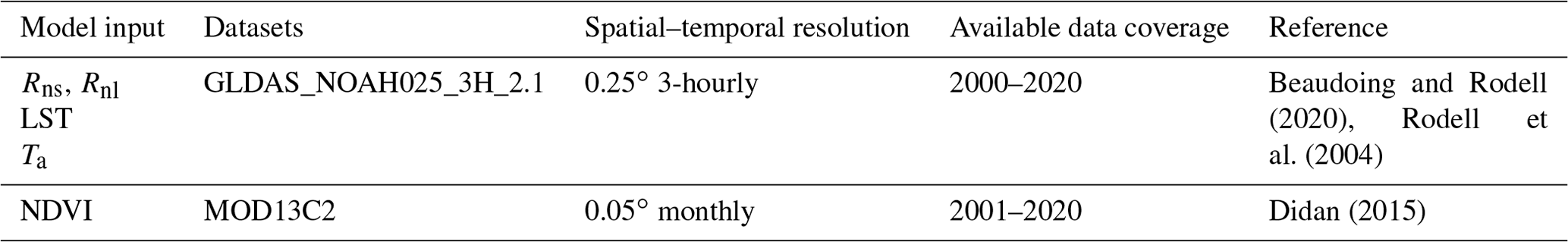
Note: R_ns: net shortwave radiation; R_nl: net longwave radiation; LST: land surface temperature; T_a: air temperature; NDVI: normalized difference vegetation index.

To remotely estimate ET at the watershed scale, Xiong and Qiu (2014) proposed a simple method to determine the reference temperature. Specifically, a pixel with the maximum temperature within a given watershed can be defined as the reference pixel. Once the reference pixel has been determined, the reference vegetation temperature, T_cr (or reference soil temperature, T_sr), can be obtained with Eq. (8) (or Eq. 9). In the global-scale application in this study, 31 terrestrial climate regions based on the Köppen–Geiger climate classification system (Kottek et al., 2006) were first divided into subregions via the principal component analysis (PCA) and K-means clustering methods, aiming to maintain relatively equivalent climate conditions within each subregion. Specifically, PCA was used to select major variables to describe regional characteristics from GLDAS meteorological factors (i.e., net radiation, air temperature, humidity, wind speed, precipitation, and air pressure) and land surface conditions (i.e., albedo, land surface temperature, NDVI, soil moisture, and soil temperature). Thereafter, these variables were used to classify the 31 climate regions through the K-means clustering method. Because of meteorology and land surface variation, the subregions varied from 90 to 110 in different months, and a reference pixel could be determined in each subregion for applying the 3T model.

$$\begin{array}{}\text{(8)}& {\displaystyle }{T}_{\mathrm{cr}}=T_{\mathrm{c},\max }=max(T_{\mathrm{c}\mathrm{1}},T_{\mathrm{c}\mathrm{2}},\mathrm{\dots },T_{\mathrm{c}i}),\text{(9)}& {\displaystyle }{T}_{\mathrm{sr}}=T_{\mathrm{s},\max }=max(T_{\mathrm{s}\mathrm{1}},T_{\mathrm{s}\mathrm{2}},\mathrm{\dots },T_{\mathrm{s}i}),\end{array}$$

where T_ci and T_si denote the vegetation surface and soil temperatures, respectively, in pixel i (i=1, 2, 3…) within each subregion.

The reference net radiation values of the soil and vegetation components, R_n,sr and R_n,cr, respectively, were assumed to be mean R_n,c and R_n,s values, respectively, within the same subregion corresponding to pixels of the upper 5 % T_s and T_c values, respectively.

$$\begin{array}{}\text{(10)}& {\displaystyle }{R}_{\mathrm{n},\mathrm{sr}}=\stackrel{\mathrm{‾}}{R_{\mathrm{n},\mathrm{s}}\left[T_{\mathrm{s},\mathrm{upper}\mathrm{5}\mathit{\%}}\right]}=\text{mean}\left(R_{\mathrm{n},\mathrm{s}\mathrm{1}},R_{\mathrm{n},\mathrm{s}\mathrm{2}},\mathrm{\dots },R_{\mathrm{n},\mathrm{s}j}\right),\text{(11)}& {\displaystyle }{R}_{\mathrm{n},\mathrm{cr}}=\stackrel{\mathrm{‾}}{R_{\mathrm{n},\mathrm{c}}\left[T_{\mathrm{c},\mathrm{upper}\mathrm{5}\mathit{\%}}\right]}=\text{mean}\left(R_{\mathrm{n},\mathrm{c}\mathrm{1}},R_{\mathrm{n},\mathrm{c}\mathrm{2}},\mathrm{\dots },R_{\mathrm{n},\mathrm{c}j}\right),\end{array}$$

where R_n,sj and R_n,cj denote the soil and vegetation net radiation values, respectively, corresponding to pixel j (j=1, 2, 3…) of the upper 5 % T_s and T_c values, respectively, within the same subregion.

The daytime ET was considered in this study. In global-scale applications, the daytime can be defined based on 3-hourly GLDAS net radiation values higher than 100 W m⁻². Then, all the 3-hourly LE (or ET) estimates can be arithmetically averaged (or summed) into daily, monthly, and annual values.

2.3 Evaluation of the performance of the 3T model

ET values estimated with the 3T model were assessed on three scales due to challenges in the validation of RS-based ET estimates (Vinukollu et al., 2011; Miralles et al., 2016; Liu et al., 2016). First, ET estimates at daily and monthly scales were validated against in situ observations retrieved from global EC flux towers covering various land cover types, as widely applied in other studies, e.g., Chen et al. (2016) and Ma et al. (2021). Due to a mismatch between the flux tower footprint and pixel resolution (0.25^∘ in this study), mean ET values in different watersheds were compared to those obtained from the water balance equation on a yearly scale. EC-based and basin-scale water-budget-based validation methods are considered the most reliable and commonly used methods. Finally, ET estimates were compared to several gridded ET products on a multi-year average scale. Statistical analysis, including Pearson's correlation coefficient (r), relative bias (RB), and root mean square error (RMSE), was employed in assessment.

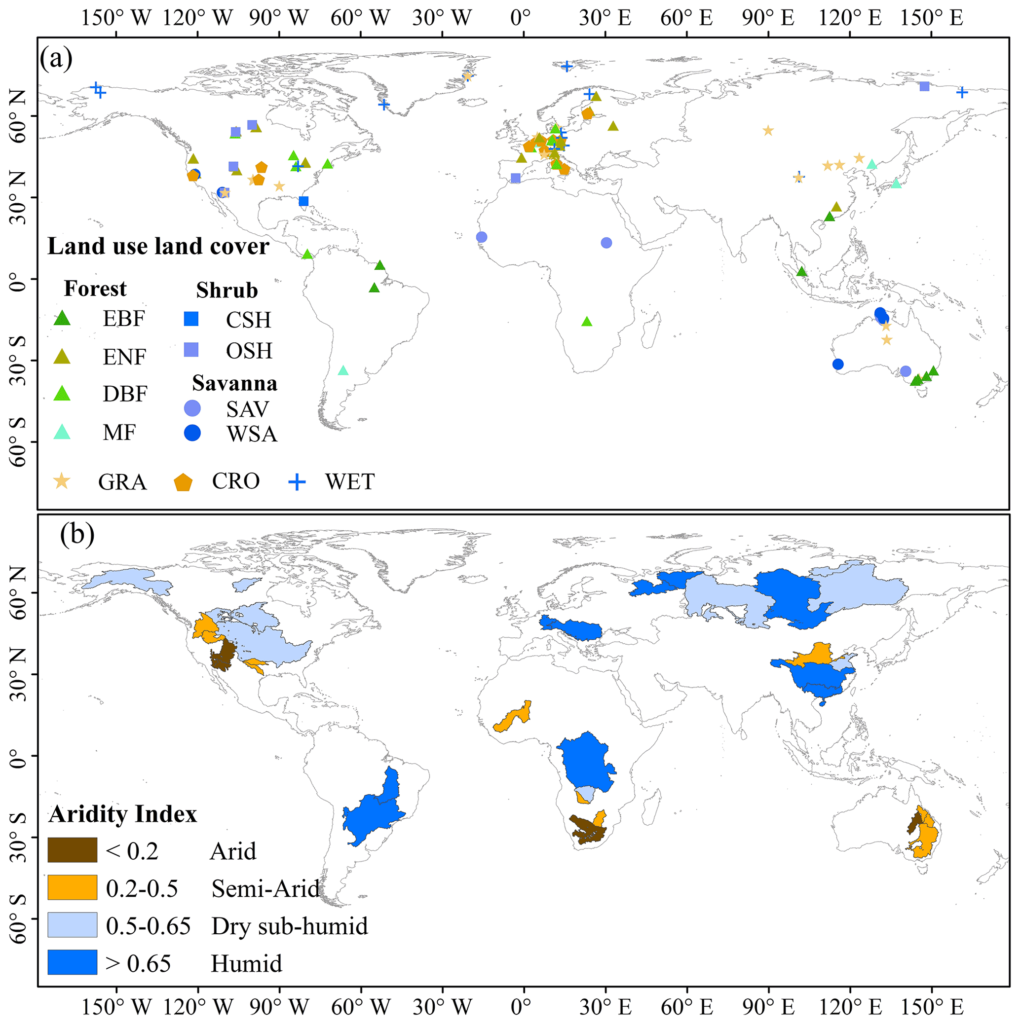
Figure 1 Locations of the eddy covariance flux towers (a) and catchments (b) used for ET validation in this study. In this study, 126 flux towers and 34 catchments are considered. CRO denotes croplands, CSH denotes closed shrublands, DBF denotes deciduous broadleaf forests, EBF denotes evergreen broadleaf forests, ENF denotes evergreen needleleaf forests, GRA denotes grasslands, MF denotes mixed forests, OSH denotes open shrublands, SAV denotes savannas, WET denotes wetlands, and WSA denotes woody savannas. The multi-year mean aridity index in each catchment is calculated as the mean annual precipitation divided by the mean annual reference ET (Trabucco and Zomer, 2018), and the catchment classification refers to the United Nations Environment Programme (UNEP, 1997).

2.3.1 Evaluation via the global eddy covariance network

ET observations of 126 flux towers within the FLUXNET network (https://fluxnet.org/, last access: 5 September 2021) were selected (Fig. 1a), and the selection process was conducted according to the following criteria. (1) A given flux tower should exhibit stable operation conditions for at least 2 consecutive years since 2001. (2) The latent heat flux (LE) was subjected to energy closure correction, and the percentage of good-quality measurement and gap-filled data should be higher than 0.7. (3) The land cover within each 0.25^∘ grid pixel containing a tower should be as homogeneous as possible (Zhang et al., 2019; Ma et al., 2021). The selected 126 EC towers were located at 26 evergreen needle leaf forest (ENF), 25 grassland (GRA), 15 cropland (CRO), 15 wetland (WET), 13 deciduous broadleaf forest (DBF), 8 evergreen broadleaf forest (EBF), 7 open/closed shrubland (OSH/CSH), 6 mixed forest (MF), 6 woody savanna (WSA), and 5 savanna (SAV) sites globally. Pixel-scale ET estimates based on the EC tower location were compared to EC tower observations.

2.3.2 Evaluation considering the water budget in global main catchments

The catchment ET (ET_wb), based on the water balance equation, has been recognized as a highly robust and credible method, particularly in relatively large catchments, on a multi-year (more than 10-year) scale (Liu et al., 2016). Hence, 34 catchments (Fig. 1b) were selected based on the following two criteria. (1) The basin area should be larger than 100 000 km² to minimize uncertainties in the measurement of water balance equation components in relatively small basins. (2) The available basin data should cover more than 10 years since 2001. ET_wb can be calculated with Eq. (12):

$$\begin{array}{}\text{(12)}& {\text{ET}}_{\mathrm{wb}}=P-R-\mathrm{\Delta }S,\end{array}$$

where P, R, and ΔS are the precipitation (mm yr⁻¹), runoff (mm yr⁻¹), and terrestrial water storage change (mm yr⁻¹), respectively, in a given catchment. Annual ΔS can be calculated as the terrestrial water storage anomaly (TWSA) difference between the Decembers of the target year and its previous year. Monthly 0.25^∘-resolution P data (full monthly data version 2020) were downloaded from the Global Precipitation Climatology Center (GPCC, http://gpcc.dwd.de/, last access: 5 October 2021) (Schneider et al., 2020). R data were acquired from the Global Runoff Data Center (GRDC, https://portal.grdc.bafg.de/, last access: 16 October 2021). Monthly 0.5^∘-resolution TWSA data were obtained from the JPL Mascon RL06 version 2.0 GRACE dataset (Watkins et al., 2015).

2.3.3 Evaluation via comparison to other commonly used global ET products

At the global scale, six commonly used ET products retrieved from different methods were selected for inter-comparison. Among the selected ET products, three products were based on the PM model with varying resistance parameterization schemes, i.e., MOD16 (version 6, Mu et al., 2011), P-LSH (Zhang et al., 2015), and PML (version 2, Zhang et al., 2019), while the remaining three products were based on the PT model (GLEAM version 3.5a; Miralles et al., 2011; Martens et al., 2017), land surface models (GLDAS version 2.1, Beaudoing and Rodell, 2020; Rodell et al., 2004), and machine learning (Fluxcom; Jung et al., 2019). All products were first resampled to 0.25^∘ via the nearest-neighbor method before comparison. Datasets covering the 2003–2013 period were used to maintain the above ET products. In the comparison process, non-vegetated areas (please refer to the Fluxcom product) were excluded due to the absence of ET data in certain products, such as the Fluxcom and MOD16 products.

Figure 2 The temporal variations in daily ET estimated from the 3T model (green line) using EC observations (gray dot). The scatter plot between EC observations and ET estimates for 1 selected year (with RMSE values at the average level) at 10 EC sites covering various biomes: (a) all 126 sites, (b1, 2) EBF_AU-Tum (36^∘ S, 148^∘ E) in 2008, (c1, 2) SAV_AU-DaS (14^∘ S, 131^∘ E) in 2009, (d1, 2) DBF_US-UMB (46^∘ N, 85^∘ W) in 2006, (e1, 2) ENF_US-Me2 (44^∘ N, 122^∘ W) in 2008, (f1, 2) OSH_US-Whs (32^∘ N, 110^∘ W) in 2012, (g1, 2) WSA_US-Ton (38^∘ N, 120^∘ W) in 2010, (h1, 2) MF_BE-Bra (51^∘ N, 5^∘ E) in 2009, (i1, 2) CRO_DE-Geb (51^∘ N, 11^∘ E) in 2008, (j1, 2) WET_CZ-wet (49^∘ N, 15^∘ E) in 2009, (k1, 2) GRA_AT-Neu (47^∘ N, 11^∘ E) in 2009.

3 Results

3.1 Performance of the 3T product versus the global EC network

At the daily scale, the 3T model-based ET estimates agreed well with the observation (N=294 058), with RMSE of 32 W m⁻² (or 1.1 mm d⁻¹) (Fig. 2a), which was comparable to other ET products, such as GLDAS (RMSE: 32 W m⁻² or 1.1 mm d⁻¹) (Fig. S1), PML (RMSE: 0.7 mm d⁻¹) (Zhang et al., 2019), and SEBS (RMSE: 1.6 mm d⁻¹) (Chen et al., 2021). Moreover, the 3T model could capture the change trend of daily ET because comparison results at 10 EC sites covering various biomes in both the Southern Hemisphere (Fig. 2b and c) and Northern Hemisphere (Fig. 2d–k) indicate that interannual variabilities of the estimates were close to that of the observed ET. A comparison at an instantaneous 3 h scale was also performed to test the ET estimates. EC observations across the world for the 15th day of each month in 2011 (N=6278) were compared because the data are too large to perform an entire comparison at a global scale. Although the RMSE (74 W m⁻²) was slightly greater than that at the daily scale (Fig. S2a), the 3T model-based ET estimates at the 3 h scale agree well with the GLDAS ET, with an r of 0.89 and a RMSE of 21 W m⁻² (Fig. S2b). The explanation is likely that high temporal data may encounter missing values, which complicates the comparison.

Figure 3 Comparison of the estimated (3T model) and measured (EC tower) monthly ET values from 2003 to 2013, where panel (a) shows the data for all 126 sites on a multi-year monthly mean (MYM) scale and panel (b) shows the data for all sites on an annual mean (AM) monthly scale. Panels (c)–(l) show all land use/land cover types on an annual monthly scale. The abbreviations in panels (c)–(l) are the same as those in Fig. 1.

At the monthly scale, the paired ET values between the 3T model and EC observations were generally distributed on both sides of the 1:1 line, revealing relatively large differences at a few points for ET values higher than 100 mm month⁻¹ and resulting in regression line slope and r values of 0.75 and 0.80, respectively (Fig. 3a). The RMSE and RB values between the ET estimates and EC-based observations reached 22.85 mm month⁻¹ and −1.2 %, respectively. If monthly data were compared, similar results could be obtained, with an RMSE value of 24.90 mm month⁻¹, an RB value of 0.7 %, and regression line slope and r values of 0.75 and 0.78, respectively (Fig. 3b). The errors in the 3T model-based ET estimates were comparable to those in the other ET products (please refer to Sect. 3.3 for details). For example, compared to EC observations, the RMSE and r values of an ET product retrieved from the process-based Breathing Earth System Simulator (BESS) model reached 23.4 mm month⁻¹ and 0.79, respectively (Jiang and Ryu, 2016). These results indicate that the ET product developed based on the 3T model agreed well with global EC observations at multi-temporal scales.

The performance of the 3T model in the different biomes was further analyzed (Fig. 3c–l). Due to data point separation in Fig. 3b, the results shown in Fig. 3c–l are similar to those shown in Fig. 3b, with slight differences among the various biomes. The 3T model performed the best at forest sites because the paired data points were more closely distributed along the 1:1 line, with slope values ranging from 0.81 to 1.05, whereas the r values ranged from 0.75 to 0.85 (Fig. 3e–h). Among the different forest cover types, the ET estimates at the MF and ENF sites exhibited a lower uncertainty, with RMSE and RB values of 20.3 mm month⁻¹ and 13.3 %, respectively, at the former sites and values of 22.8 mm month⁻¹ and 10.4 %, respectively, at the latter sites, followed by DBF (RMSE = 24.2 mm month⁻¹ and RB = 25.8 %) and EBF sites (RMSE = 29.7 mm month⁻¹ and RB = 4.6 %). The 3T model performance at the shrubland sites was similar to that at the MF sites (RMSE = 20.6 mm month⁻¹ and RB = 9.2 %) but with lower slope and r values of 0.53 and 0.60, respectively (Fig. 3i). At the sites of the remaining land use/land cover (LULC) types, the 3T model yielded lower ET estimates than the EC observations as the RB value ranged from −6.1 % to −33.8 % (Fig. 3c, d, and j to l). Among these sites, the 3T model exhibited the lowest bias at the GRA sites, with slope, r, and RMSE values of 0.71, 0.82, and 21.4 mm month⁻¹, respectively (Fig. 3j), followed by the SAV (slope = 0.67, r=0.83, and RMSE = 27.7 mm month⁻¹) (Fig. 3k), CRO (slope = 0.61, r=0.78, and RMSE = 27.9 mm month⁻¹) (Fig. 3c), WET (slope = 0.65, r=0.74, and RMSE = 28.3 mm month⁻¹) (Fig. 3d), and WSA sites (slope = 0.49, r=0.70, and RMSE = 31.7 mm month⁻¹) (Fig. 3l). The 3T model performance among the different biomes, with a maximum RMSE value of 31.7 mm month⁻¹, was comparable to that of the other methods based on the above comparison to EC observations, with RMSE values ranging from 30 to 42.9 mm month⁻¹, as reported by Carter and Liang (2018), Zhang et al. (2019), and Peng et al. (2021). These results suggest that the 3T model performed with an acceptable accuracy across the various biomes.

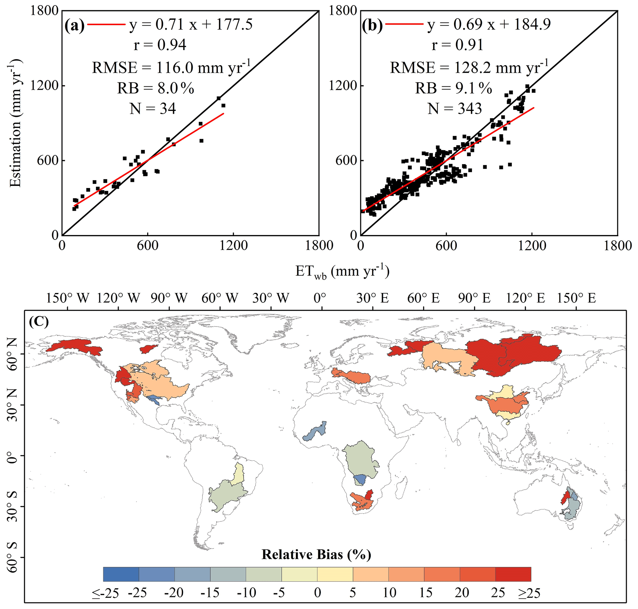
Figure 4 Comparison of the annual model-estimated (3T model) and water-balance-based ET values during the 2003–2013 period: (a) multi-year mean annual scale, (b) annual scale, and (c) relative bias (RB) in each basin.

3.2 Performance of the 3T product versus the water budget in global catchments

Multi-year (2003–2013) average ET values for 34 relatively large watersheds were obtained with the 3T model and compared to water balance ET (ET_wb) data. The estimated mean ET value was 514.5 mm yr⁻¹, with a standard deviation of 211 mm yr⁻¹, whereas the mean ET_wb value reached 476.5±280 mm yr⁻¹. The mean ET difference reached only 38 mm yr⁻¹, indicating that the ET estimates obtained with the 3T model were similar to the ET_wb values. The scatter plots shown in Fig. 4a and b at multi-year and annual scales, respectively, also confirmed that these two types of ET values agreed well, with r values of 0.94 and 0.91, respectively. The regression line slope at the multi-year scale was 0.71, with RMSE and RB values of 116 mm yr⁻¹ and 8.0 %, respectively (Fig. 4a), whereas the values reached 0.69, 128 mm yr⁻¹, and 9.1 %, respectively, at the annual scale (Fig. 4b). Figure 4c shows the 3T model performance in each watershed in terms of RB. The RB values in nearly 70 % of the watersheds were relatively low, within ±25 %, indicating satisfactory performance of the 3T model in these watersheds. However, the 3T model overestimated ET in approximately 21 % of all watersheds, with RB values greater than 60 % (the red color in Fig. 4c). These river basins were mainly located at high latitudes (approximately 60^∘ N) with relatively low ET_wb values (133±50 mm yr⁻¹). ET overestimation in these regions was not only observed in this study, but was also observed in other ET comparison-based studies, such as Ma et al. (2021). A possible reason for the higher uncertainty may be that a higher bias occurs in the hydrological (e.g., runoff) and gridded meteorological (e.g., precipitation) data employed in the water balance equation due to the scarcity of in situ observational stations in these regions (Ma et al., 2021). Nonetheless, the above results generally suggest that the 3T model performance was comparable to that of the water balance equation.

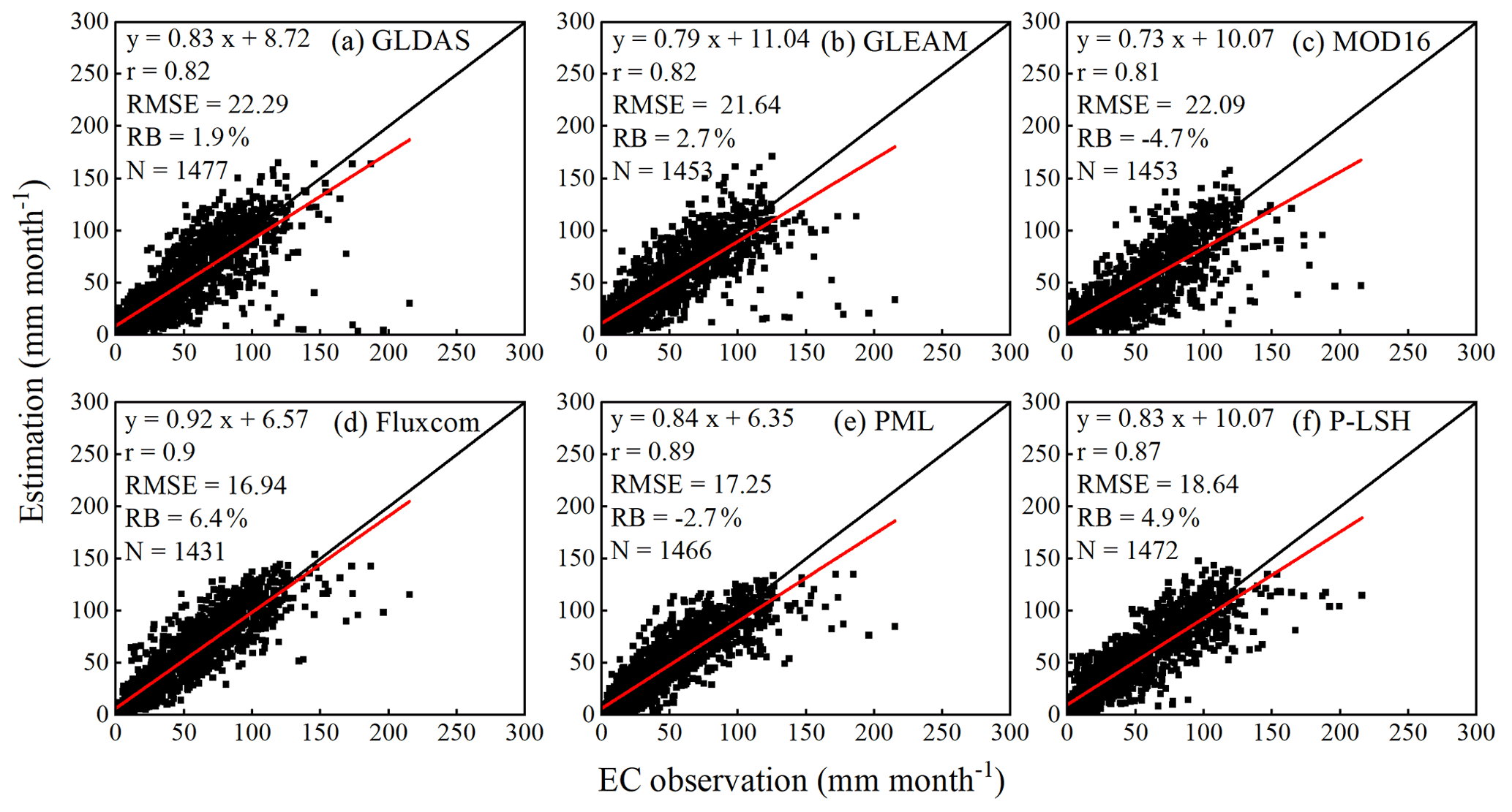
Figure 5 Validation of six commonly used ET products (GLDAS, PML, P-LSH, GLEAM, Fluxcom, and MOD16) against EC tower observations. The data are monthly average ET values over the 2003–2013 period and are the same as those used in Fig. 3a.

3.3 Comparison of the 3T product to other global ET products

To further assess the performance of the 3T model across the various terrestrial land types, 3T model-based ET estimates were cross-validated against six global ET products during the 2003–2013 period.

When EC observation data were adopted as a reference, 3T model-based ET estimates were comparable to GLDAS, GLEAM, and MOD16 data in terms of r and RMSE, with values of 0.8 and 22 mm month⁻¹, respectively (Figs. 3a and 5a–c). Although the slope of the regression line (0.75, as shown in Fig. 3a) between the 3T model-based ET estimates and observations was slightly lower than that between the ET estimates and GLDAS (0.83, as shown in Fig. 5a) and GLEAM data (0.79, as shown in Fig. 5b) and slightly higher than that between the ET estimates and MOD16 data (0.73, as shown in Fig. 5c), the absolute RB value of the 3T model was lower than that of the GLDAS (1.9 %, as shown in Fig. 5a), GLEAM (2.7 %, as shown in Fig. 5b), and MOD16 products (−4.7 %, as shown in Fig. 5c). The remaining three products, i.e., Fluxcom, PML, and P-LSH, exhibited limited comparative advantages, with an r value of 0.9, a slope higher than 0.8 (0.92, 0.84, and 0.83, respectively), and an RMSE value ranging from 16.9 to 18.6 mm month⁻¹.

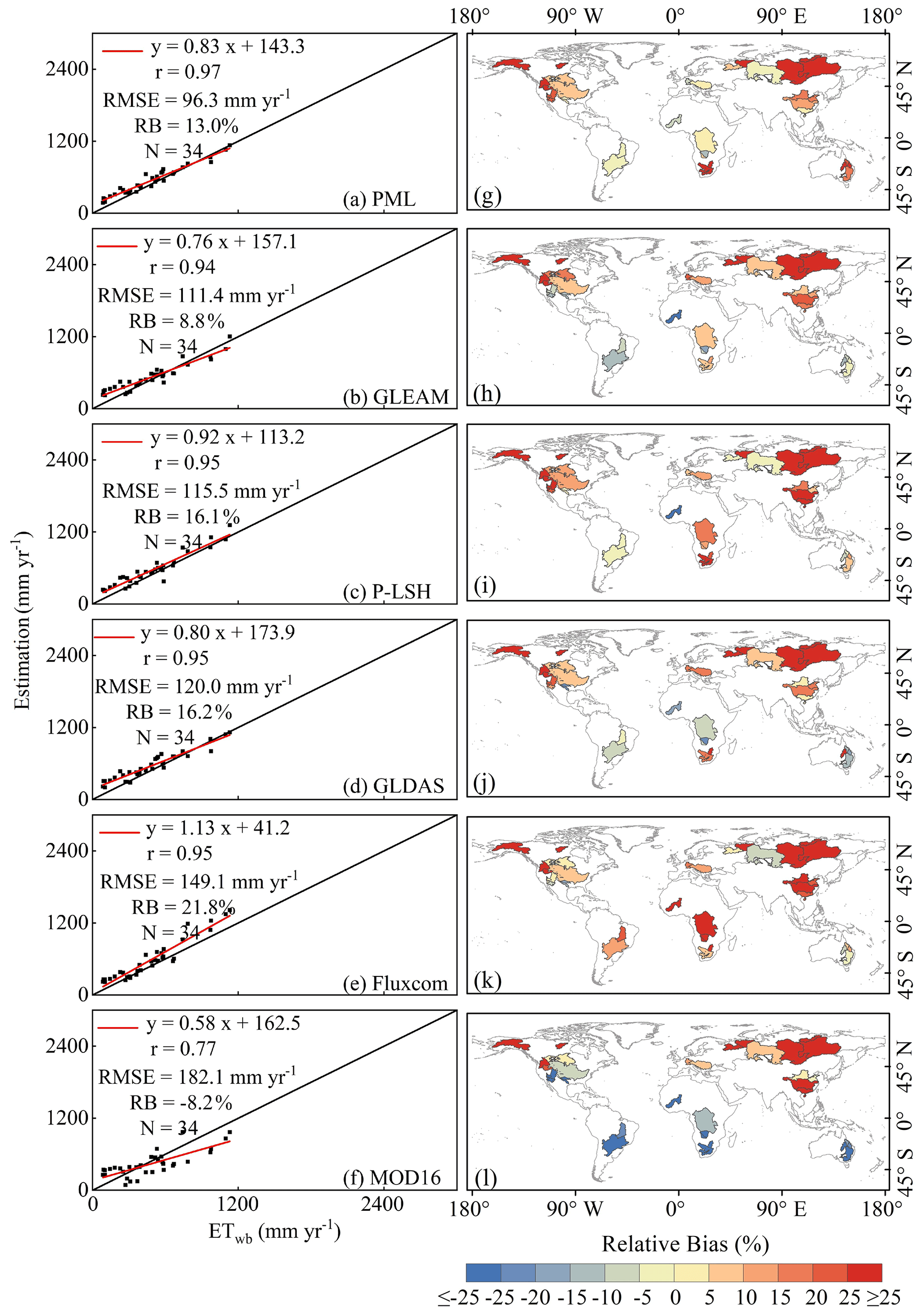
Figure 6 Validation of six commonly used ET products (GLDAS, PML, P-LSH, GLEAM, Fluxcom, and MOD16) against values obtained with the catchment water balance approach. The data are yearly average values over the 2003–2013 period. The left column shows mean annual values, and the right column shows the RB in each catchment.

When ET_wb values were adopted as a reference, although the 3T model performance was slightly lower than that of the PML, GLEAM, and P-LSH products in terms of RMSE, with a value of 116 mm month⁻¹ versus values of 96, 111, and 115 mm month⁻¹, respectively (Figs. 4a and 6a–c), the 3T model performed better than did the GLDAS (RMSE = 120 mm month⁻¹), Fluxcom (RMSE = 149 mm month⁻¹), and MOD16 products (RMSE = 182 mm month⁻¹) (Fig. 6d–f). In terms of the regression line between the ET estimates and ET_wb, except for the relatively low performance of MOD16, for slope and r values of 0.58 and 0.77, respectively, r values of the other ET products were greater than 0.94 and exhibited a slight difference, with a maximum difference of 0.03, but the slope (0.71, as shown in Fig. 4a) of the regression line between the ET_wb values and 3T model-based ET estimates was lower than that between the ET_wb values and Fluxcom (1.13), P-LSH (0.92), PML (0.83), GLDAS (0.80), and GLEAM data (0.76) (Fig. 6). However, the absolute RB, with a value of 8 % (Fig. 4a), of the 3T model was the smallest, while the absolute RB values of the other six products were greater than 8 %, ranging from 8.2 % to 21.8 % (Fig. 6).

Via comparison of the terrestrial (excluding Antarctica) ET values retrieved from the various ET products, the mean ET value of the 3T model reached 546 mm yr⁻¹ during the 2003–2013 period, whereas the mean ET values obtained with the MOD16, PML, GLEAM, Fluxcom, GLDAS, and P-LSH products reached 468, 542, 544, 549, 551, and 551 mm yr⁻¹, respectively.

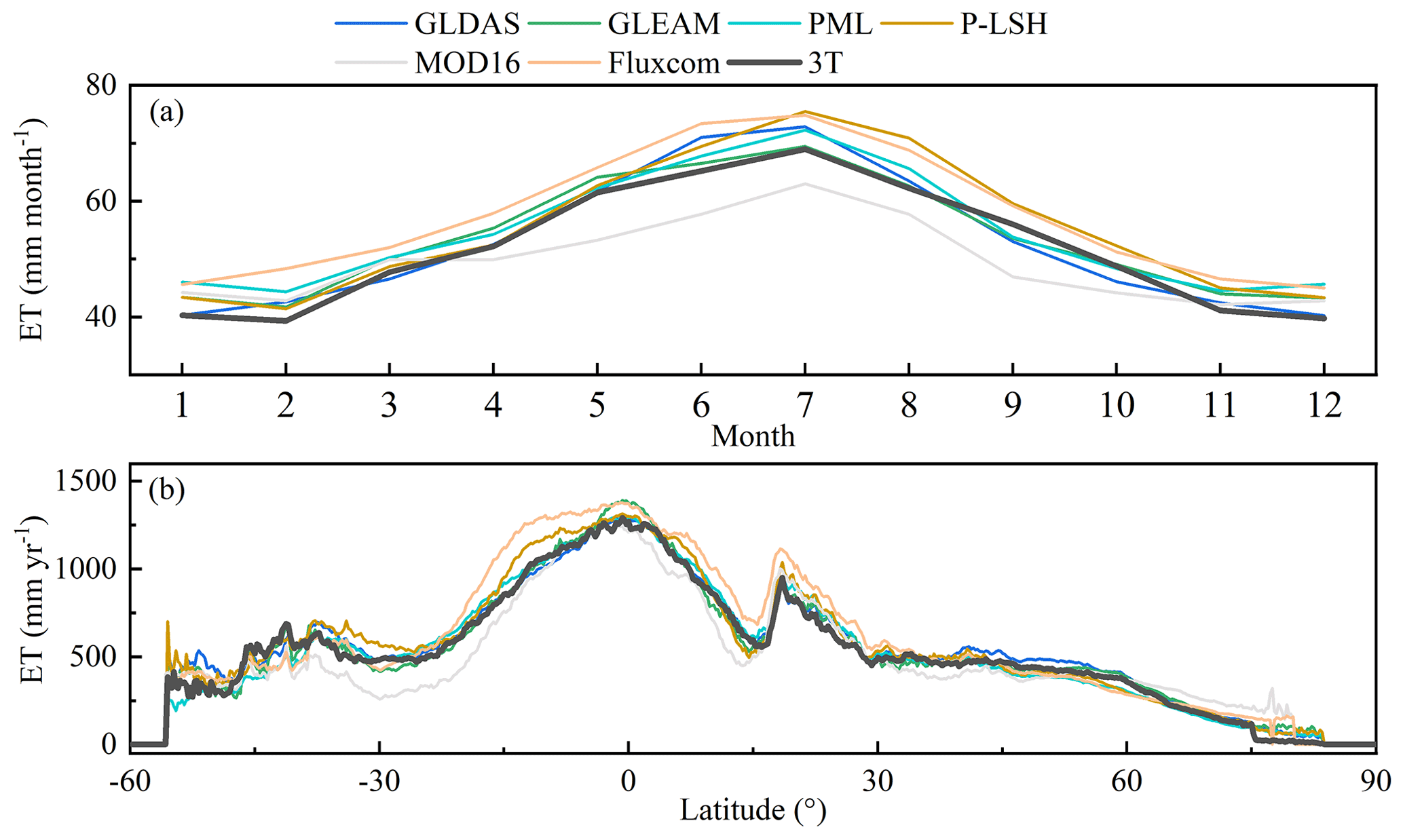
Figure 7 (a) Monthly variation and (b) annual latitudinal distributions of the multi-year (2003–2013) mean ET value estimated with the 3T model (black line) and six ET products in vegetated areas (mainly excluding Greenland, Antarctica, and desert areas, according to Jung et al., 2019).

In terms of interannual variation (excluding Antarctica, Greenland, and desert areas according to Jung et al., 2019), the 3T model-based estimates were similar to the other six ET products, with an increasing trend from January (approximately 40 mm month⁻¹) to July (approximately 65 mm month⁻¹) and then a decreasing trend through the following months (Fig. 7a). The latitudinal distribution of the values obtained with each ET product was also determined, and the changing trend of the 3T model-based ET values was similar to that of the values obtained with the six considered ET products (Fig. 7b). Specifically, the highest terrestrial ET values occurred at the Equator, with values ranging from 1251 to 1390 mm yr⁻¹ (1293 mm yr⁻¹ for the 3T model), and the ET value decreased towards the North Pole and South Pole. In the Northern Hemisphere, ET attained a second peak at approximately 20^∘, with values ranging from 934 to 1111 mm yr⁻¹ (950 mm yr⁻¹ for the 3T model), whereas a third peak occurred from 37 to 45^∘ (the third peak varied among the different ET products) in the Southern Hemisphere, with values ranging from 562 to 706 mm yr⁻¹ (690 mm yr⁻¹ for the 3T model). This ET peak distribution trend was correlated with the global vegetation distribution. However, it should be noted that the ET values obtained with the 3T model were generally lower than those obtained with the ET products between approximately 30^∘ S and 45^∘ N (except MOD16), and a large discrepancy in ET estimates occurred, particularly between approximately 17^∘ S and 17^∘ N, where the difference could exceed 350 mm yr⁻¹. These results suggest that even though the ET products are similar, the ET estimates in certain areas may differ, and uncertainty may exist in ET estimates in these regions.

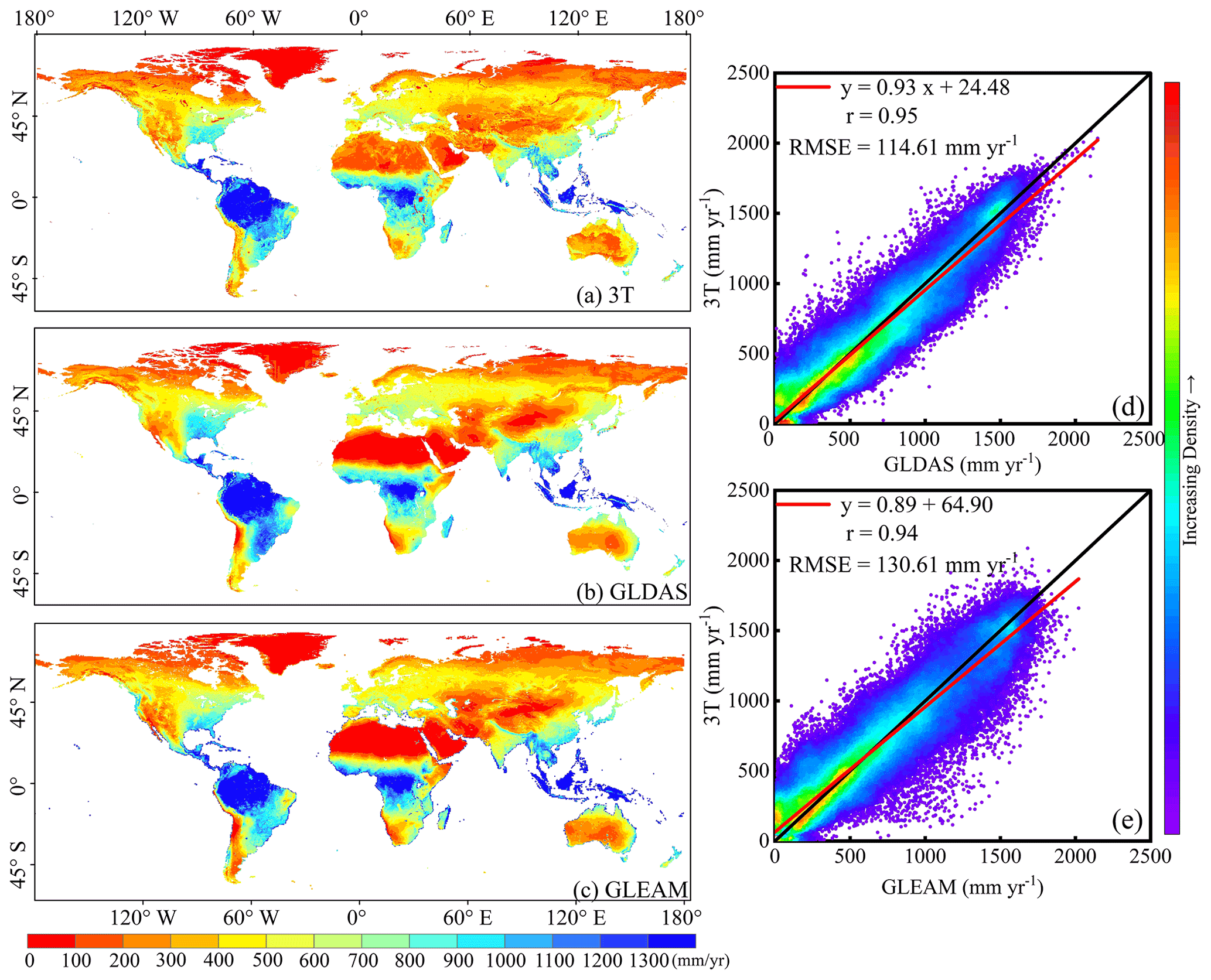
Figure 8 Spatial pattern and pixel-to-pixel comparison of multi-year (2003–2013) global mean annual ET rates among the 3T model, the GLDAS, and GLEAM. Left column: spatial ET distribution of (a) 3T model-, (b) GLDAS-, and (c) GLEAM-based ET values. Right column: pixel-to-pixel comparison of ET values between (d) the 3T model and the GLDAS and (e) the 3T model and GLEAM.

Figure 9 RMSE and r of pixel-to-pixel (0.25^∘ resolution) comparison of multi-year (2003–2013) mean annual ET values among the 3T model and six products in vegetated areas (mainly excluding Greenland, Antarctica, and desert areas, according to Jung et al., 2019).

Pixel-by-pixel comparison of the various ET products was also conducted. To overcome the influence of the resampling method on the obtained ET values, only GLDAS and GLEAM data, sharing the same spatial resolution as the 3T model-based estimates (0.25^∘), are shown in Fig. 8. The left column shows the global land ET distribution, and the 3T model-based ET values generally exhibited a similar distribution to that of the ET values obtained with the two ET products, as shown in Fig. 8. However, obvious differences existed, especially in arid regions such as the Sahara, the Middle East, Mongolia, and the southeast of the Qinghai–Tibet Plateau, where the 3T model-based ET estimates were higher than the values obtained with the two ET products. The scatter plots in the right column of Fig. 8 reveal that the 3T model-based ET estimates were very similar to the GLDAS-based ET values. Moreover, the slope of the regression line between the 3T model- and GLDAS-based ET values was 0.93, with r and RMSE values of 0.95 and 114.6 mm yr⁻¹, respectively (Fig. 8d), whereas the values reached 0.89, 0.94, and 130.6 mm yr⁻¹, respectively, between the 3T model and GLEAM (Fig. 8e). RMSE and r statistics between the 3T model-based ET estimates and the values obtained with each ET product were visualized in a heatmap (Fig. 9) in which the darker the blue color is, the higher the r value and the lower the RMSE value are. Overall, the 3T model-based ET product is consistent with the other six products, with r ranging from 0.89 (compared to MOD16) to 0.96 (compared to GLDAS) and RMSE ranging from 108.5 (compared to the GLDAS) to 177.7 (compared to MOD16) mm yr⁻¹. Interestingly, it was obvious that the 3T model-based, GLDAS, and PML products with the same model inputs were highly consistent according to the higher r and lower RMSE values (the corresponding blue cubes are in the bottom left of Fig. 9), while the ET products calibrated or upscaled based on EC towers, i.e., PML, P-LSH, and Fluxcom, were highly consistent (the corresponding blue cubes are in the top right of Fig. 9).

The abovementioned results indicate that the 3T model-based ET estimates were comparable to the data obtained with the commonly used global ET products.

Table 2 Information on the typical ET products used to cross-validate the ET estimates of the 3T model in this study.

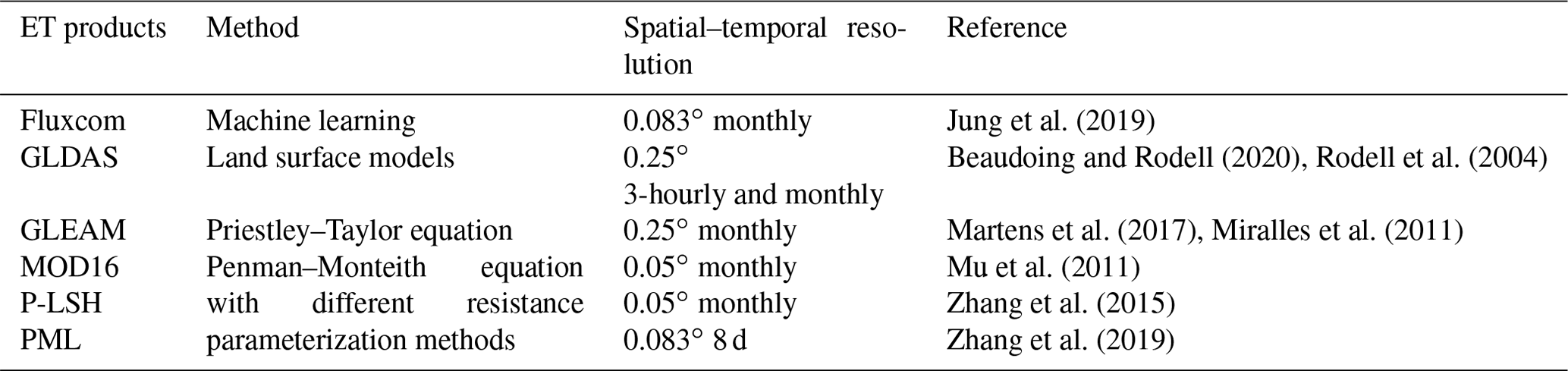
Table 3 Multi-year (2003–2013) average ET values considering the water depth (mm yr⁻¹) and volume (km³ yr⁻¹) of the different products used in this study for the global land surface.

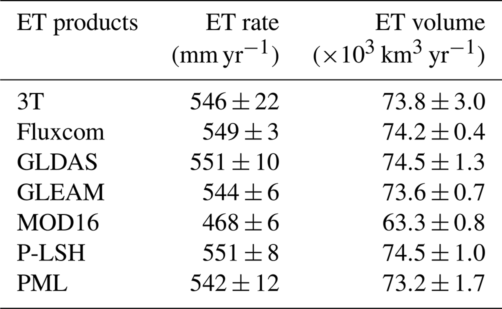
Note: the global land surface has an area of 1.35×10⁸ km², excluding Antarctica. Fluxcom and MOD16 do not provide ET values in Greenland and desert areas.

4 Discussion

4.1 Characteristics of the global terrestrial ET product based on the 3T model

As indicated in Sect. 3, the 3T model-based global terrestrial ET product agreed well with ground observations and was comparable to other commonly used ET products. Particularly, the determined global terrestrial (excluding Antarctica) ET volume (in units of 10³ km³ yr⁻¹) based on 3T model-based estimates reached 73.8 from 2003 to 2013, which is not only consistent with that determined based on the other ET products (excluding MOD16), as indicated in Sect. 3.3, ranging from 73.2 to 74.5 (Table 3), but also consistent with values reported in other studies, e.g., 72.3±0.9, as obtained with a complementary relationship-based ET product from 1982 to 2016 (Ma et al., 2021), and 71.1, as determined with a water-balance- and machine-learning-based ET product from 1982 to 2009 (Zeng et al., 2014).

It should be noted that the 3T model differed from the methods used to estimate ET in the adopted ET products, as listed in Table 2. In particular, the 3T model excludes resistance and requires no parameter calibration. Resistance terms are unavoidable in PM models, which could lead to high uncertainty in ET estimates (Zhao et al., 2020; Cao et al., 2021). As described in Sect. 3.3, the MOD16, P-LSH, and PML products, based on the PM equation with varied resistance parameterization methods, exhibited obvious differences (e.g., 300 mm yr⁻¹ at a few locations, as shown in Fig. 7b) and performed differently via a comparison to ground observations. This occurred because the canopy resistance is difficult to estimate, in addition to the empirical relationship adopted in the estimation process. These empirical equations are site- and biome-specific equations and normally require calibration (Mu et al., 2011; Zhang et al., 2015, 2019). Because a large number of EC tower sites are used for calibration in resistance estimation in P-LSH and PML, these two products performed better than MOD16, using only 46 sites (Figs. 5 and 6). Nonetheless, calibration typically requires observational data, while limited in situ observations restrict accurate calibration of biome-specific coefficients on a global scale. A recent study confirmed that models requiring no calibration could decrease the uncertainty in global ET estimates (Ma et al., 2021). The obtained results indicate that the 3T model-based ET product achieved a lower uncertainty than that achieved by MOD16 retrieved from the PM equation with a complex resistance parameterization scheme and limited calibration and that the 3T model-based ET product was comparable to P-LSH and PML developed from the PM equation with adequate calibration during resistance parameterization.

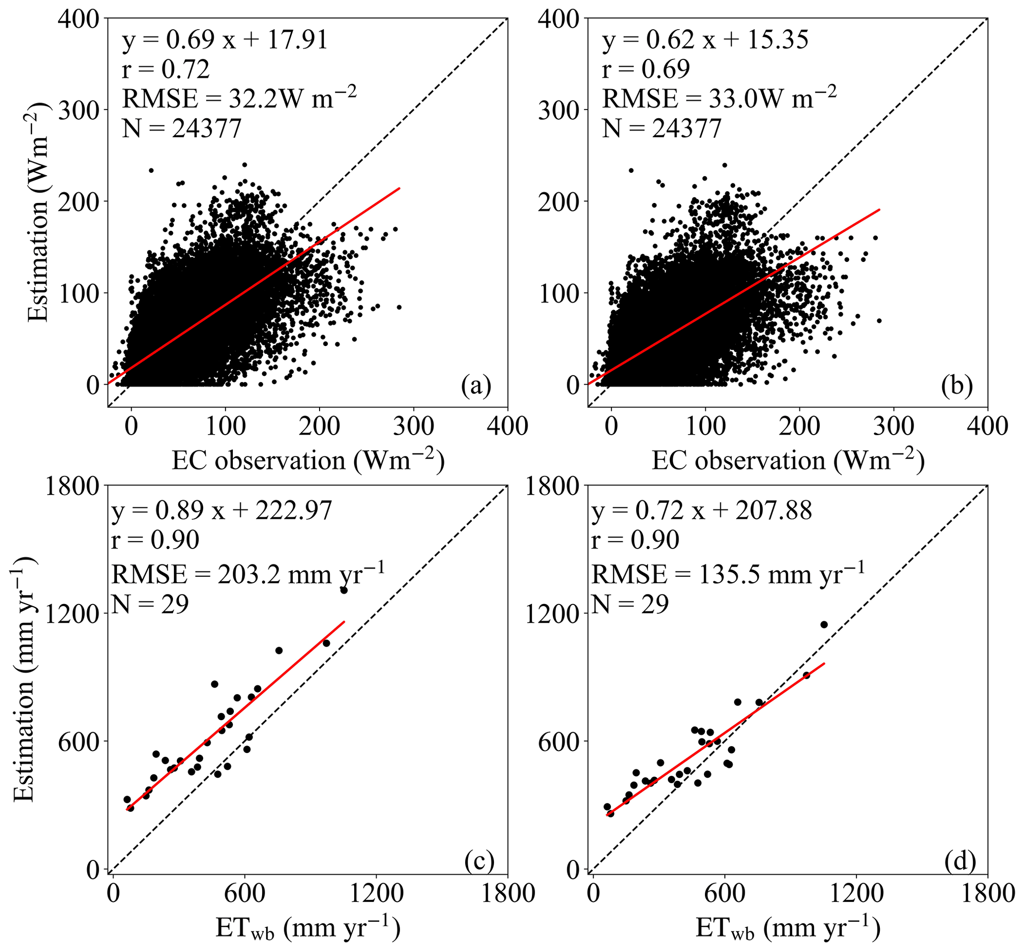
Figure 10 Comparison of the estimated (3T model) and measured ET values in 2011 (daily ET from EC tower and annual ET from the water balance equation). The left column shows ET estimates using Köppen–Geiger climate regimes with 31 subregions at the daily (a) and annual (c) scales, respectively, whereas the right column is the same but with ET estimates using 90–110 subregions.

Although the 3T model-based ET estimates suffer from the domain size when determining the reference site, the uncertainty may be limited. We tested the difference between the 3T model-based ET values estimated using two different regimes with different subregions and sizes. Specifically, Köppen–Geiger climate regimes with 31 subregions and detailed subregions with numbers of 90–110 were used. In general, the two groups of daily ET estimates in 2011 showed little difference, with mean ET values of 47 and 42 W m⁻², respectively, and were close to the EC observation, with RMSE values of 32 and 33 W m⁻² (Fig. 10a and b, respectively). At a yearly scale, however, the 3T model-based ET estimates from 90 to 110 subregions (Fig. 10d) were much closer to the water balance ET than those estimates using 31 subregions (Fig. 10c). The results indicate that the smaller the domain size of a region where the reference parameters were obtained, the more accurate the 3T model, which is consistent with our previous findings (Xiong et al., 2015, 2019).

In addition, the 3T model-based global terrestrial ET product required fewer data in terms of model inputs than those required by the adopted ET products, as listed in Table 2. Specifically, the 3T model requires net radiation, soil heat flux, air temperature, LST, and vegetation index (i.e., NDVI) data to decompose the radiation (or LST) components of vegetation and soil. For example, PM-based ET estimation requires wind speed and VPD data in addition to net radiation, soil heat flux, and air temperature data. However, wind speed and VPD data, especially the former, exhibit high heterogeneity in space, and current commonly used reanalysis datasets contain high uncertainty; e.g., the difference in wind speed can exceed 5 m s⁻¹ among several products (Yang et al., 2019), thus increasing bias in global ET products. While a model with a higher complexity may better describe the ET process, a satisfactory model performance normally depends on abundant data, not only regarding model inputs, but also regarding model (or parameter) calibration (Medici et al., 2012; Wu et al., 2020). Otherwise, a relatively simple model with fewer input datasets could be more reasonable; e.g., the GLEAM product based on the PT method, a simplified version of the PM equation, outperformed the PM-based MOD16 product in this and other studies (e.g., Cao et al., 2021). Although the performance of the 3T model-based ET product was similar to that of the GLEAM product, an empirical parameter, namely, the PT coefficient, is required in the PT-based GLEAM product. In estimation with the GLEAM product, the PT coefficient was set to 0.8 for tall canopies and 1.26 for short vegetation and bare soil, respectively (Miralles et al., 2011), but the value varies among the different biomes (e.g., Komatsu, 2005), especially on a short timescale (daily) (Guo et al., 2015). In fact, the input datasets of the 3T model are commonly available with an adequate credibility (Bao and Zhang, 2013; Cao et al., 2022; Fu and Wang, 2014; Ji et al., 2015; Peng et al., 2019; Xu et al., 2019; X. Zhang et al., 2016; Zhou et al., 2017), resulting in easy model application.

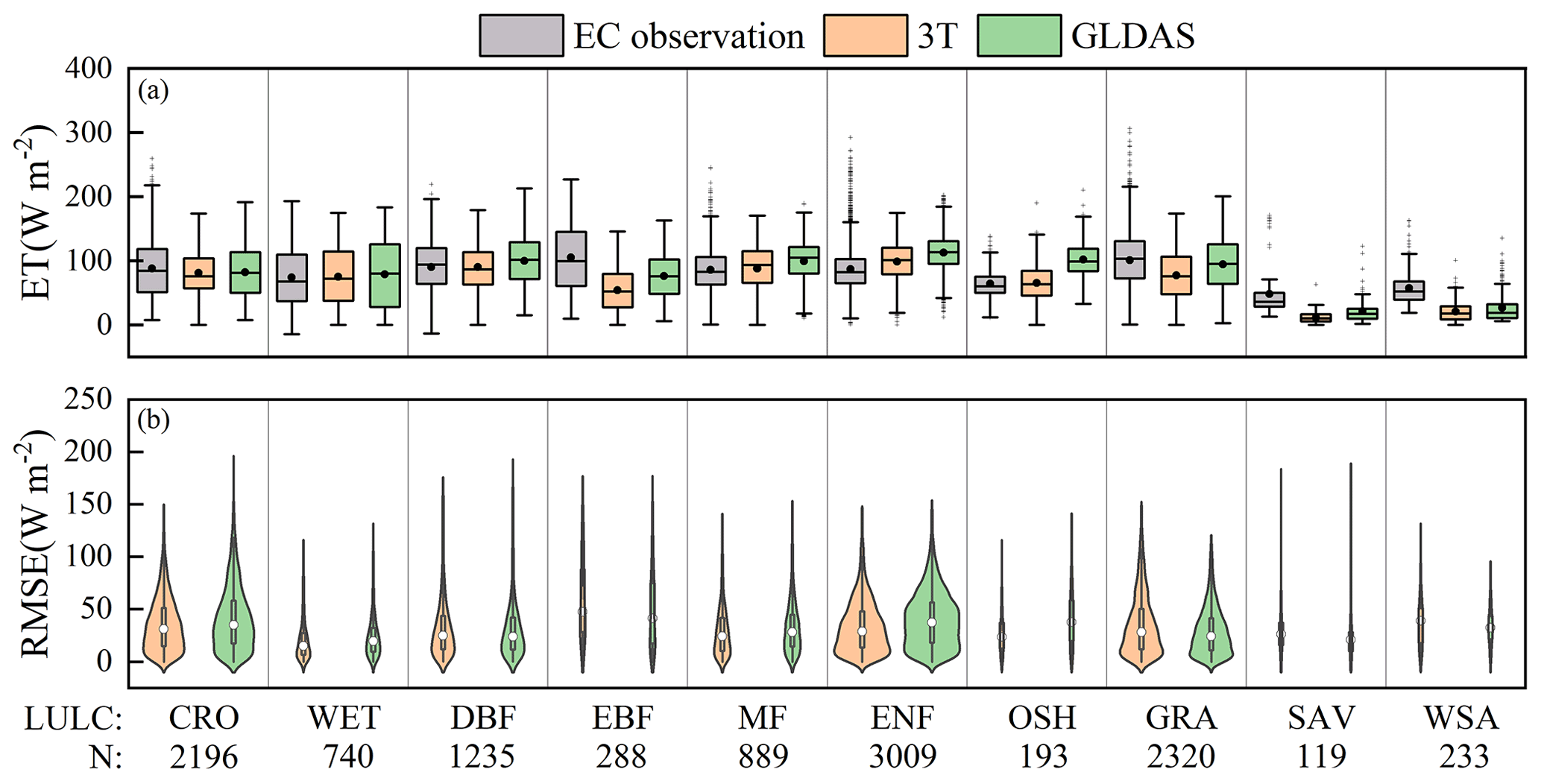
Figure 11 Monitoring performance of the 3T model-based terrestrial ET product under extreme heat conditions in the different biomes. The daily ET is shown in energy units. In the box plot (a), the black point indicates the mean, while the central line in the box indicates the median value. The edges of the box indicate the 25th and 75th percentiles, and the whiskers indicate the outlier values. In the violin plot (b), the white point indicates the median value, and a wider violin plot indicates denser data for the same RMSE value. N denotes the number of data points.

4.2 The 3T model-based terrestrial ET product for extreme weather condition monitoring

Although the 3T model is the most sensitive to the LST among the various model inputs (Xiong and Qiu, 2011), this characteristic may result in a suitable model ability in capturing ET variation during extreme-temperature events such as heat waves and flash droughts. Since both the frequency and damage extent of heat waves and flash droughts are increasing, these extreme weather conditions have attracted extensive attention worldwide (IPCC, 2022). For instance, Senay et al. (2020) applied a temperature-sensitive model, i.e., the Operational Simplified Surface Energy Balance (SSEBop) model, to estimate ET and used its anomalies to successfully detect the 2011/2012 drought in the southern–central United States and the 2005 drought in Australia. However, this study mainly used relatively low ET values to qualitatively describe droughts, while few studies focused on the accuracy of ET estimates under similar extreme conditions (i.e., heat and drought conditions). Hence, this section further examines the 3T model-based terrestrial ET product for extreme weather condition monitoring by validating its performance against EC flux tower observations under extreme heat, extreme atmospheric drought, and extreme soil drought conditions. These three types of extreme hazards were defined according to daily observations from 2001 to 2020 retrieved from FLUXNET and GLDAS reanalysis data (version 2.1) based on corresponding site locations: (1) extreme heat conditions occur when the daily T_a at a given EC tower site is higher than the 95th percentile of the daily T_a in GLDAS data, (2) extreme atmospheric drought conditions occur when the daily VPD at a given EC tower location is higher than the 95th percentile of the daily VPD in GLDAS data, and (3) extreme soil drought conditions occur when the daily soil moisture matches the 5th percentile of EC tower data. It should be mentioned that some data points indicated both extreme heat and extreme atmospheric drought conditions. These points were designated as extreme heat conditions instead of extreme atmospheric drought conditions. Finally, there remained 11 213 data points across 80 sites, 19 687 data points across 112 sites, and 12 338 data points across 95 sites representing extreme heat, extreme atmospheric drought, and extreme soil drought conditions, respectively. GLDAS estimates, with a high temporal resolution in the monitoring of extreme events (Liu et al., 2019) and the same spatiotemporal input datasets such as those employed for the 3T model, were also used in the analysis.

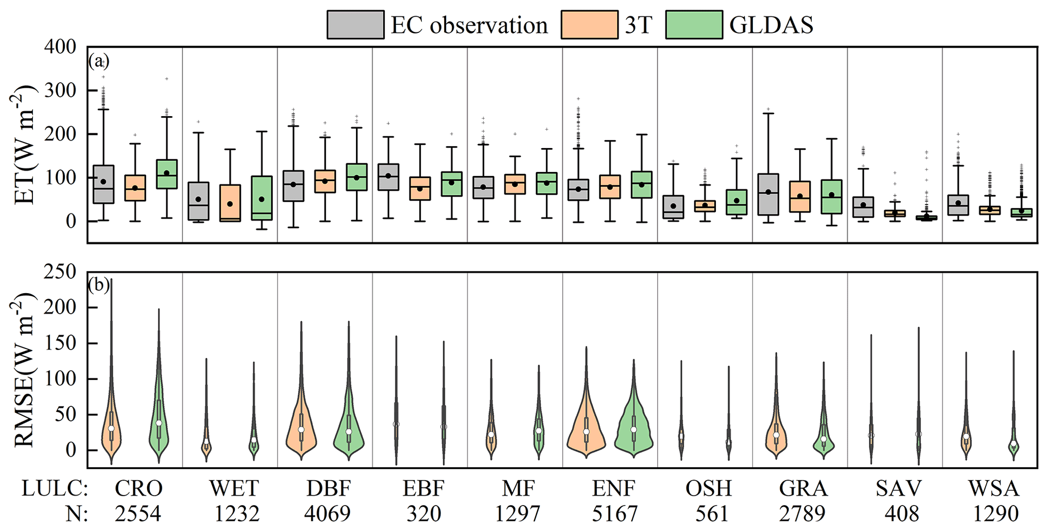
Figure 12 Monitoring performance of the 3T model-based terrestrial ET product under extreme atmospheric drought conditions in the different biomes. The symbols are the same as those in Fig. 11.

Under extreme heat conditions (Fig. 11), although the 3T model-based ET product exhibited various performance levels in the different biomes, the product generally yielded results closely agreeing with observations. In terms of the mean ET value, extreme heat conditions at the DBF, WET, OSH, MF, CRO, and ENF sites were best captured with the 3T model-based ET product (Fig. 11a), with a maximum difference of 11.9 W m⁻² from EC observations, followed by the GRA, WSA, SAV, and EBF sites with difference values ranging from 24.0 to 51.1 W m⁻². The GLDAS performed similarly to the 3T model-based ET product but with a notably higher bias than that of EC observations. The RMSE violin plots shown in Fig. 11b further verify the above statement because the RMSE values obtained with the 3T model-based ET product, with median values of 23.6, 29.0, 15.3, 31.2, and 24.4 W m⁻² at the OSH, ENF, WET, CRO, and MF sites, respectively, were much smaller than those obtained with the GLDAS (37.9, 37.4, 19.9, 35.2, and 28.2 W m⁻², respectively). The maximum RMSE values obtained with the 3T model-based ET product were also smaller than those obtained with the GLDAS, 48.3, 20.6, 20.2, 15.6, and 14.1 W m⁻² lower at the CRO, DBF, OSH, WET, and MF sites, respectively. These results indicate that the 3T model-based ET product could accurately capture the low ET values under extreme heat conditions in most biomes and performed better than did the GLDAS.

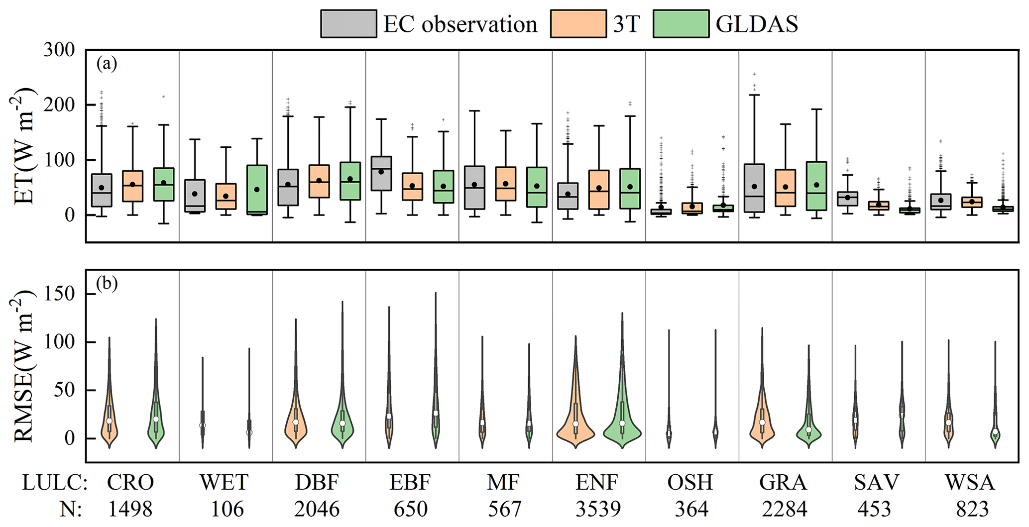
Figure 13 Monitoring performance of the 3T model-based terrestrial ET product under extreme soil drought conditions in the different biomes. The symbols are the same as those in Fig. 11.

Under extreme atmospheric drought conditions (Fig. 12), in terms of the mean ET value, the 3T model-based ET product suitably captured extreme atmospheric drought conditions at the OSH, ENF, MF, DBF, GRA, WET, CRO, and WSA sites (Fig. 12a), with a maximum difference of 14.5 W m⁻² from EC observations, followed by the SAV and EBF sites, with difference values ranging from 18.2 to 29.7 W m⁻². The GLDAS also performed similarly to the 3T model-based ET product but with a higher bias over EC observations, which was further confirmed by the RMSE violin plots shown in Fig. 12b. The median RMSE values obtained with the 3T model-based ET product (the white points in Fig. 12b) reached 30.7, 22.2, 26.2, 21.0, and 12.7 W m⁻² at the CRO, MF, ENF, SAV, and WET sites, respectively, while the values obtained with the GLDAS reached 38.4, 27.4, 29.0, 22.9, and 14.4, respectively. The above results indicate that the 3T model-based ET product could accurately capture the low ET values under extreme atmospheric drought conditions at the CRO, MF, ENF, and WET sites and performed better than did the GLDAS.

Under extreme soil drought conditions (Fig. 13), in terms of the mean ET value, the 3T model-based ET product suitably captured extreme soil drought conditions at the GRA, OSH, MF, WSA, WET, CRO, DBF, and ENF sites (Fig. 13a), with a maximum difference of 7.2 W m⁻² from EC observations, followed by the SAV and EBF sites with difference values ranging from 13.2 to 25.5 W m⁻². The median RMSE values obtained with the 3T model-based ET product (the white points in Fig. 13b) at the SAV, EBF, CRO, OSH, and ENF sites reached 18.9, 23.2, 18.2, 5.4, and 15.3 W m⁻², respectively, while the values obtained with the GLDAS reached 23.8, 26.4, 20.0, 6.9, and 15.8, respectively. In addition, compared to the GLDAS, the maximum RMSE values obtained with the 3T model-based ET product at the ENF, EBF, CRO, WET, and SAV sites were reduced by 55.6, 18.5, 14.0, 9.3, and 3.0 W m⁻², respectively. The acquired results indicate that the 3T model-based ET product could accurately capture the low ET values under extreme atmospheric drought conditions at the CRO, EBF, and ENF and performed better than did the GLDAS.

It should be noted that the 3T model-based ET product exhibited a good performance in crop ET estimation under these three types of extreme conditions. Compared to the GLDAS, the 3T model-based ET estimates were closer to the considered EC observations and exhibited smaller errors, as described in the previous discussion. Considering that CRO areas are important for human society but highly sensitive to extreme events (Xia et al., 2021) and crop ET estimation suffers from more challenges than those encountered in the other natural biomes (He et al., 2019; Melton et al., 2021), the sensitivity of the 3T model to the temperature ensures that the method could provide very high potential ability for crop ET estimation, especially under extreme temperature conditions.

5 Data availability

The daily and monthly ET dataset presented and analyzed in this article has been released and is available for free download from the Science Data Bank (https://doi.org/10.57760/sciencedb.o00014.00001, Xiong et al., 2022). The dataset is published under the Creative Commons Attribution 4.0 International (CC BY 4.0) license.

6 Conclusions

A global ET product, derived from reanalysis and RS data based on the 3T model, was provided with daily and 0.25^∘ resolutions from 2001 to 2020. The product was thoroughly assessed via direct evaluation against FLUXNET EC tower data at the daily and monthly scales and water-balance-based catchment ET data at the annual scale, in addition to cross-validation against six commonly used global ET products. The 3T model-based ET estimates generally agreed well with the above observations. Furthermore, the 3T model exhibited a very high potential for accurate ET estimation under extreme weather conditions. Since the 3T model requires only a few input parameters (i.e., R_n, LST, and T_a) without the need for parameter calibration, it could be concluded that the model is easy and simple to apply, and the proposed ET product could provide reasonable information to support water-cycle-related studies.