British Antarctic Survey's aerogeophysical data: releasing 25 years of airborne gravity, magnetic, and radar datasets over Antarctica

Over the past 50 years, the British Antarctic Survey (BAS) has been one of the major acquirers of aerogeophysical data over Antarctica, providing scientists with gravity, magnetic, and radar datasets that have been central to many studies of the past, present, and future evolution of the Antarctic Ice Sheet. Until recently, many of these datasets were not openly available, restricting further usage of the data for different glaciological and geophysical applications. Starting in 2020, scientists and data managers at BAS have worked on standardizing and releasing large swaths of aerogeophysical data acquired during the period 1994–2020, including a total of 64 datasets from 24 different surveys, amounting to ∼ 450 000 line-km (or 5.3 million km²) of data across West Antarctica, East Antarctica, and the Antarctic Peninsula. Amongst these are the extensive surveys over the fast-changing Pine Island (BBAS 2004–2005) and Thwaites (ITGC 2018–2019 & 2019–2020) glacier catchments, and the first ever surveys of the Wilkes Subglacial Basin (WISE-ISODYN 2005–2006) and Gamburtsev Subglacial Mountains (AGAP 2007–2009). Considerable effort has been made to standardize these datasets to comply with the FAIR (findable, accessible, interoperable and re-usable) data principles, as well as to create the Polar Airborne Geophysics Data Portal (https://www.bas.ac.uk/project/nagdp/, last access: 18 July 2022), which serves as a user-friendly interface to interact with and download the newly published data. This paper reviews how these datasets were acquired and processed, presents the methods used to standardize them, and introduces the new data portal and interactive tutorials that were created to improve the accessibility of the data. Lastly, we exemplify future potential uses of the aerogeophysical datasets by extracting information on the continuity of englacial layering from the fully published airborne radar data. We believe these newly released data will be a valuable asset to future glaciological and geophysical studies over Antarctica and will significantly extend the life cycle of the data. All datasets included in this data release are now fully accessible at https://data.bas.ac.uk (British Antarctic Survey, 2022).

1 Introduction

As one of the fastest changing environments on Earth, Antarctica has been at the epicentre of scientific research since the early 1960s. Understanding the past, present, and future of the Antarctic Ice Sheet is of special interest, particularly in the context of rapid climatic changes already affecting large parts of the Antarctic Peninsula and threatening the stability of the West Antarctic Ice Sheet (WAIS; IPCC, 2021). One way to quantify how the ice sheet will respond to these changes is to conduct studies of englacial and basal properties of the ice using geophysical techniques such as gravity, magnetic, and radar. By studying the bedrock topography beneath an ice sheet, we can better estimate where a retreating ice stream is more likely to stabilize or destabilize further (Holt et al., 2006; Vaughan et al., 2006; Tinto and Bell, 2011; Ross et al., 2012; Morlighem et al., 2020) and how landforms or subglacial water-routing systems can affect the flow regime of ice streams (Bell et al., 2011; Wright et al., 2012; Schroeder et al., 2013; Ashmore and Bingham, 2014; Siegert et al., 2014; Young et al., 2016; Napoleoni et al., 2020). By studying the subglacial geology, we can better understand magmatic, tectonic, and sedimentary influences on ice flow over timescales of hundreds, thousands or even millions of years (Bell et al., 1998; Blankenship et al., 2001; Studinger et al., 2001; Bamber et al., 2006; Bell et al., 2006; Jordan et al., 2010; Bingham et al., 2012), and quantify the influence of geothermal heat flux on ice dynamics (Schroeder et al., 2014; Jordan et al., 2018). Finally, the use of gravity techniques enables us to better understand the bathymetry beneath fast-changing ice shelves and ice-stream fronts and quantify areas of high sensitivity (Greenbaum et al., 2015; Millan et al., 2017; Tinto et al., 2019; Jordan et al., 2020).

Since the mid-1960s, the British Antarctic Survey (BAS) has been involved in acquiring aerogeophysical data with a particular focus on radar-data acquisition using a 35 and 60 MHz radio-echo sounder developed at the Scott Polar Research Institute (Robin et al., 1970), and, in collaboration with the Technical University of Denmark, using slightly improved versions of the same analogue radar system until the early 1990s (Robin et al., 1977). The subsequent development of an in-house digital radar system at BAS in 1993–1994 (Corr and Popple, 1994), and accompanying gravity and magnetic instruments, allowed for the first surveys over West Antarctica's Evans Ice Stream to be conducted in 1994–1995, marking the start of modern digital aerogeophysical surveying of the Antarctic by BAS. Further improvements in survey techniques and instruments have allowed BAS to develop its aerogeophysical capabilities further and become one of the leaders in aerogeophysics over the Antarctic.

Since the mid-1990s, aerogeophysical datasets acquired by BAS have played a vital role in understanding past and current ice-dynamical and lithospheric processes over the Antarctic Ice Sheet. In total, BAS flew 24 survey campaigns between 1994 and 2020, representing a total of ∼ 450 000 line-km of aerogeophysical data over the Antarctic Peninsula as well as over the WAIS and the East Antarctic Ice Sheet (EAIS) (Fig. 1, Table 1). The total cumulative survey coverage since 1994 is 5.3 million km², equivalent to > 30 % of the total area of the Antarctic Ice Sheet (14.2 million km²). Many of these surveys were acquired as part of large international collaborative projects such as the International Polar Year Antarctica's Gamburtsev Province Project (AGAP), the European Space Agency (ESA) PolarGAP project, and the US–UK International Thwaites Glacier Collaboration (ITGC), amongst others. Importantly, much of the data acquired since then have been central to the output of large international science groups, such as the Scientific Committee on Antarctic Research (SCAR) BEDMAP (I/II/III), ADMAP (I/II), AntArchitecture, and IBCSO projects (Lythe et al., 2001; Arndt et al., 2013; Fretwell et al., 2013; Golynsky et al., 2018).

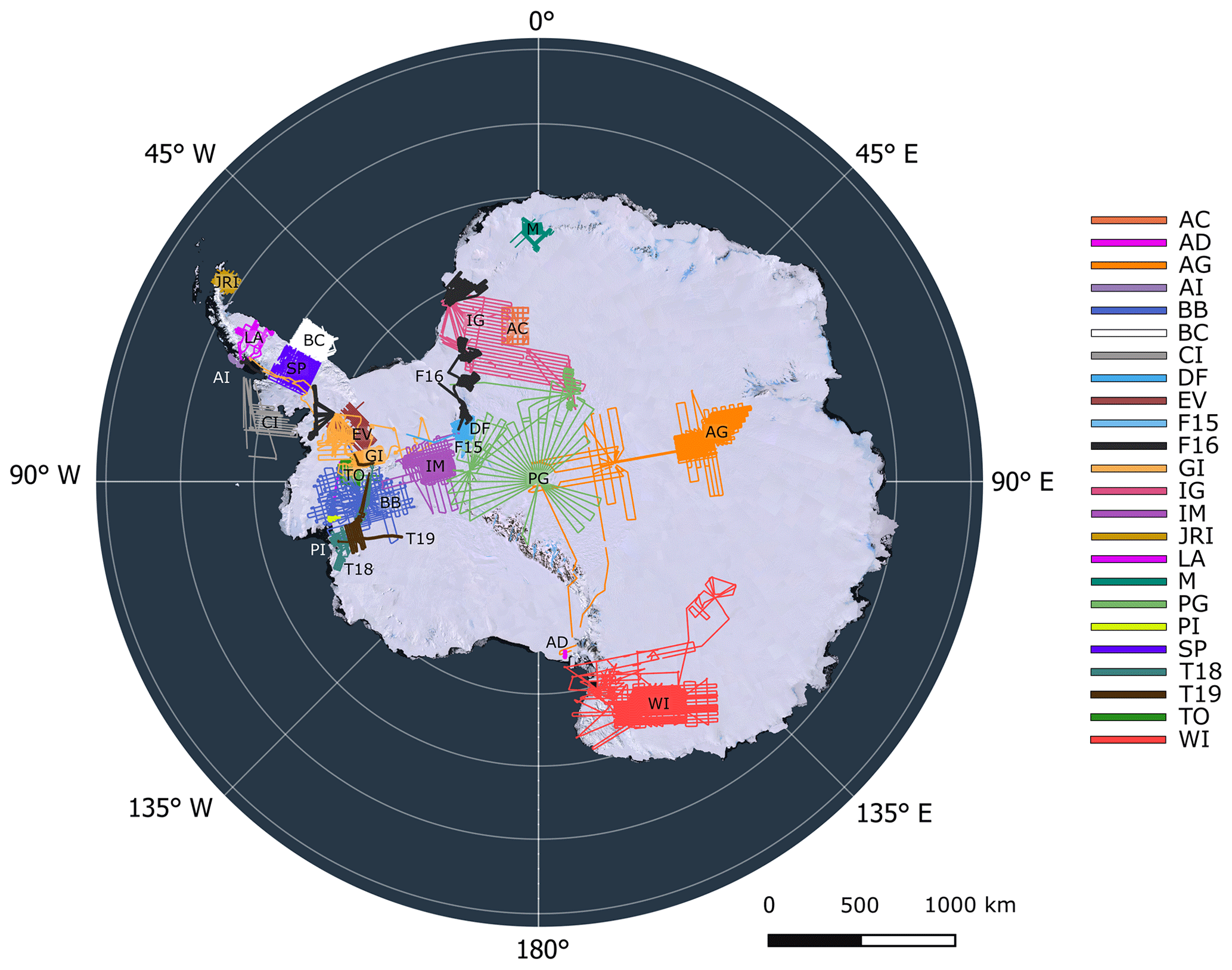
Figure 1 Map showing all the published datasets included in this data release. The colours are the same as those used on the data portal interface. Abbreviations are as follows: AC: AFI Coats Land (2001–2002); AD: Andrill HRAM (2008–2009); AG: AGAP (2007–2009); AI: Adelaide Island (2010–2011); BB: BBAS (2004–2005); BC: Black Coast (1996–1997); CI: Charcot Island (1996–1997); DF: DUFEK (1998–1999); EV: EVANS (1994–1995); F15: FISS 2015 (2015–2016); F16: FISS–EC–Halley 2016 (2015–2016); GI: GRADES-IMAGE (2006–2007); IG: ICEGRAV (2012–2013); IM: IMAFI (2010–2011); JRI: James Ross Island (1997–1998); LA: Larsen Ice Shelf (1997–1998); M: MAMOG (2001–2002); PG: PolarGAP (2015–2016); PI: Pine Island Glacier Ice Shelf (2010–2011); SP: SPARC (2002–2003); T18: ITGC (2018–2019); T19: ITGC (2019–2020); TO: TORUS (2001–2002); WI: WISE-ISODYN (2005–2006). The legend on the right-hand side of the figure shows the colour corresponding to each survey. The background image is from the Landsat Image Mosaic of Antarctica (LIMA; Bindschadler et al., 2008).

Despite the importance of these surveys for understanding the Antarctic cryosphere and tectonics, until now the underlying data have been relatively inaccessible to wider scientific communities due to the scale of the data-management task required. This lack of accessibility has hampered the ability of the wider research community to extract further valuable information from these datasets. In 2020, a collaborative project between the UK Polar Data Centre (PDC, https://www.bas.ac.uk/data/uk-pdc/, last access: 18 July 2022) and the BAS Airborne Geophysics science team was set up to improve the FAIR-ness (Wilkinson et al., 2016) of these data. The main objectives of this collaboration were to comply with national and international policies on data sharing and accessibility, foster new collaborations, and allow the further re-use of these data beyond the lifespan of the science projects.

This paper presents the result of this successful collaboration between data managers and scientists to standardize and release most of BAS' aerogeophysical data acquired to date using modern instruments from 1994 onwards. Data acquired prior to this, while particularly useful to long-term monitoring of ice sheet conditions, are much more challenging and time-consuming to update to modern standards (see Schroeder et al., 2019; Sect. 5.3), and are thus not included in the data release discussed here. Section 2 of this paper reviews the main scientific findings from each survey flown between 1994 and 2020. Section 3 describes the various instruments and techniques used to acquire and process the data. Section 4 outlines the format and data publishing strategy for our datasets following the FAIR data principles, as well as the creation of a new data portal and interactive, open-access tutorials. Finally, Sect. 5 provides a case study for the re-usability of the newly released aerogeophysical data, as well as suggestions on future uses of the data portal and aspirations for future data releases.

2 Background

The following section reviews the main scientific findings related to the acquisition of aerogeophysical data from BAS for the period 1994–2020 and is divided into two sub-sections: (i) findings from surveys conducted pre-2004 using older aerogeophysical instruments and for which the fully processed 2-D radar data are not published as part of this data release (see Table 1, Sect. 5.3), and (ii) surveys conducted post-2004 using the PASIN-1 (2004–2015) and PASIN-2 (2015–2020) radar systems and more modern data-acquisition methods. Figures 2–3 present the wide-ranging datasets of gravity and magnetic anomalies, bed elevation and ice thickness, and 2-D radar profiles ensuing from the surveys discussed in Sect. 2.1. and 2.2.

2.1 Aerogeophysical surveys for the period 1994–2004

The first surveys conducted by BAS since the mid-1990s involved extensive gravity and magnetic surveying of the western and eastern Antarctic Peninsula and Weddell Sea Embayment. Surveys over Evans Ice Stream (1994–1995), Black Coast (1996–1997), Charcot Island (1996–1997), and James Ross Island (1997–1998) (Fig. 1, Table 1) provided new insights into the history of crustal boundaries between the eastern Antarctic Peninsula and the Filchner Block (Ferris et al., 2002), evidence of crustal thinning below Evans Ice Stream (Jones et al., 2002), and new understanding of the magmatic and tectonic processes around the Mount Haddington stratovolcano on James Ross Island (Jordan et al., 2009). A further study covering the Larsen Ice Shelf (Antarctic Peninsula) was conducted conjointly by BAS and the Instituto Antártico Argentino in 1997–1998. The radar data acquired during this survey were used in ocean (Holland et al., 2009) and firn-density (Holland et al., 2011) models to improve our understanding of ice–ocean interactions and ice-surface elevation changes on the ice shelf. In 1998–1999, extensive aeromagnetic surveying of the Dufek Massif (West Antarctica/East Antarctica) revealed the presence of a Jurassic dike swarm that likely acted as a magma transport and feeder system to the Ferrar Large Igneous Province (Ferris et al., 2003). In 2001–2002, an additional survey was flown as part of the initiative, Targeting ice-stream Onset Regions and Under-ice Systems (TORUS), to assess the factors controlling the dynamics of the Rutford Ice Stream using gravity, magnetic, and radar instruments over a high-resolution grid spacing of ∼ 10 km (Vaughan et al., 2008). Lastly, for the WAIS, the 2002–2003 Superterranes in the Pacific Margin Arc (SPARC) campaign over northern Palmer Land (Antarctic Peninsula) used gravity and magnetic instruments to reveal subglacial imprints of crustal growth linked with the Gondwana margin (Ferraccioli et al., 2006).

Over East Antarctica, two surveys conducted in 2001–2002 acquired detailed gravity, magnetic, and radar measurements over Slessor Glacier (as part of the Antarctic Funding Initiative (AFI) Coats Land survey) and Jutulstraumen Ice Stream (as part of the Magmatism as a Monitor of Gondwana breakup survey; MAMOG). The AFI Coats Land survey, a UK initiative between BAS and the University of Bristol, provided the first accurate measurements of ice thickness and bed elevation in the area (Rippin et al., 2003a) (Fig. 2), and led to the discovery of a ∼ 3 km thick sedimentary basin associated with a weak till layer at the bed which enhances basal motion and affects the flow regime of this part of the EAIS (Rippin et al., 2003a; Bamber et al., 2006; Shepherd et al., 2006). The MAMOG survey revealed the presence of a subglacial Jurassic continental rift in the area of western Dronning Maud Land, providing early evidence for the initial Gondwana breakup (Ferraccioli et al., 2005a, b).

2.2 Aerogeophysical Surveys for the Period 2004–2020

Building on the surveys prior to 2004, which were relatively small in areal extent, BAS began surveying larger areas from the mid-2000s onwards (Table 1), primarily due to enhanced international collaborations and improvements in data acquisition and instruments, which led to data being acquired both at higher resolution and over larger spatial scales. The acquisition strategy was to collect data from multiple geophysical sensors mounted on BAS' Twin Otter aircraft across every survey, giving a holistic view of vast and previously unsurveyed regions (Figs. 4–5). The core sensor suite included gravity and magnetic instruments used to understand the geological nature of the subglacial basins and mountains along with their tectonic structure, together with the radar system used to map ice thickness and bed elevation. The development of a new radar system, the Polarimetric Airborne System INstrument (PASIN) (PASIN-1, 2004–2015) (see Sect. 3.1.3), and an improved version of the same system (PASIN-2, 2015–2016 onwards), allowed for the efficient collection of high-quality digital radar data for BAS-led campaigns in the Antarctic.

We divide the findings from these surveys into two sub-sections (Sect. 2.2.1 for surveys between 2004 and 2015 and Sect. 2.2.2 for surveys between 2015 and 2020) to reflect the acquisition of data prior to and following the upgrade of the PASIN system (see Sect. 3.1.3).

2.2.1 2004–2015

The first mission to utilize the PASIN-1 radar system was the 2004–2005 BBAS survey of Pine Island Glacier, which aimed to characterize the subglacial conditions of this sensitive glacier of West Antarctica (Vaughan et al., 2006). This survey provided two key findings: (a) the discovery of a deep subglacial trough, 500 m at its deepest point and 250 km long, through which Pine Island Glacier flows; and (b) the existence of well-constrained valley walls, which would likely provide a buffer against a potential catastrophic collapse of the WAIS via Pine Island Glacier (Vaughan et al., 2006). Further studies utilizing this dataset focused primarily on bed characteristics and the subglacial hydrology of the catchment (Rippin et al., 2011; Napoleoni et al., 2020; Chu et al., 2021), as well as tracking englacial layers and quantifying past accumulation rates (Corr and Vaughan, 2008; Karlsson et al., 2009, 2014; Bodart et al., 2021). The survey was also conducted simultaneously with another covering the Thwaites Glacier catchment led by the University of Texas Institute for Geophysics and the National Science Foundation of the United States (Holt et al., 2006), enabling a comparison of the surveying capabilities where the surveys overlapped (e.g. Chu et al., 2021).

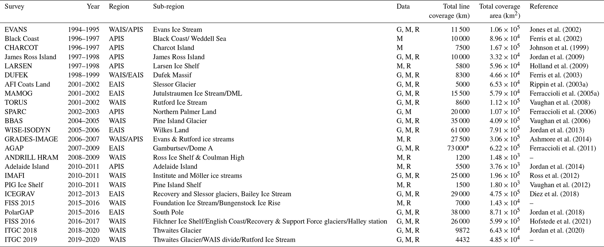
Table 1 Information on the period, region, sub-region, type of data acquired, total line coverage (km), total coverage area (km²), and key reference for each survey included in this data release. For “Data”, the abbreviations are as follows: gravity (G), magnetic (M), radar (R). For “Regions”, abbreviations are as follows: APIS (Antarctic Peninsula Ice Sheet), EAIS (East Antarctic Ice Sheet), WAIS (West Antarctic Ice Sheet). “DML” stands for Dronning Maud Land and “PIG” for Pine Island Glacier. The total area in km² is calculated as a cumulative total area of the spatial footprint of the survey's minimum and maximum extents. ^* For AGAP, the data release only consists of the BAS-acquired data, which represents approximately half of the total (∼ 120 000 km) survey coverage from the whole AGAP expedition (see Sect. 2.2.1).

Following on from the BBAS data, the suite of geophysical instruments on board the BAS Twin Otter aircraft were used to survey the Wilkes Subglacial Basin, Dome C, and the Transantarctic Mountains as part of the 2005–2006 WISE-ISODYN survey between BAS and the Italian Programma Nazionale di Ricerche in Antartide (Bozzo and Ferraccioli, 2007; Corr et al., 2007; Ferraccioli et al., 2007; Jordan et al., 2007). This project revealed, for the first time, the crustal architecture of the Wilkes Subglacial Basin (Ferraccioli et al., 2009; Jordan et al., 2013) and the distribution of a well-preserved subglacial sedimentary basin underlying the Wilkes catchment (Frederick et al., 2016). The following year, the 2006–2007 survey, Glacial Retreat in Antarctica and Deglaciation of the Earth System – Inverse Modelling of Antarctica and Global Eustasy (GRADES-IMAGE), comprising surveys over the transitional area between the Antarctic Peninsula and the WAIS, provided detailed information on subglacial properties of Evans Ice Stream (Ashmore et al., 2014). Ice-thickness measurements along the grounding line were also used as key calibration for the Landsat-derived “ASAID” grounding-line product (Bindschadler et al., 2011), and englacial layers through Bungenstock Ice Rise were used to assess ice-divide stability and the wider ice-flow history and stability of the WAIS's Weddell Sea sector during the Holocene (Siegert et al., 2013).

Over two austral field seasons from 2007 to 2009, AGAP, coordinated as part of the fourth International Polar Year between the UK, USA, Germany, Japan, Australia and China, comprised a comprehensive survey of the interior of the EAIS, yielding important aerogeophysical data used to interrogate the origin and geophysical characteristics of the Gamburtsev Subglacial Mountains. Significant scientific discoveries generated by the AGAP survey included observations of widespread freeze-on at the bottom of the ice which leads to thickening of the EAIS from the base (Bell et al., 2011), a thick crustal root formed during the Proterozoic eon (1 Gyr ago) surrounded by a more recent ∼ 2500 km-long rift system (Ferraccioli et al., 2011), and the existence of ancient pre-glacial fluvial networks at the present ice bed which confirmed the presence of the Gamburtsev Subglacial Mountains prior to the start of glaciation at the Eocene–Oligocene climate boundary (ca. 34 Ma) (Rose et al., 2013; Creyts et al., 2014).

Between 2008 and 2011, three surveys utilized the magnetic and radar instruments on board the BAS Twin Otter to conduct high-spatial-resolution surveying of Coulman High on Ross Ice Shelf as part of the Antarctic Drilling – High Resolution Aeromagnetic (ANDRILL HRAM) project, Adelaide Island (Antarctic Peninsula), and Pine Island Glacier Ice Shelf (West Antarctica). The 2010–2011 Adelaide Island survey provided high-resolution aeromagnetic data to underpin a better understanding of the complex magmatic structure of the Antarctic Peninsula Cenozoic arc/forearc boundary (Jordan et al., 2014). The Pine Island Glacier Ice Shelf survey of the same year revealed a network of sinuous subglacial channels, 500 to 3000 m wide and up to 200 m high, in the ice-shelf base, which, combined with surface and basal crevasses formed as a result of the basal melting, could lead to structural weakening of the shelf in the future (Vaughan et al., 2012).

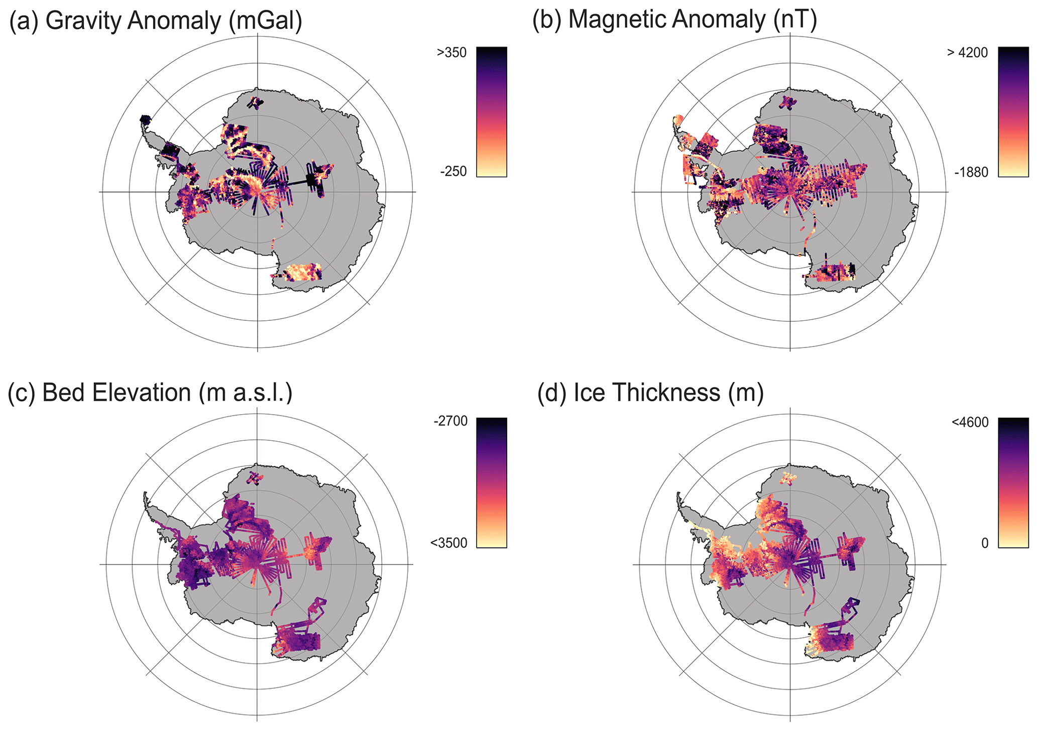
Figure 2 Maps of gravity, magnetic, and radar (bed elevation and ice thickness) point measurements for all surveys published as part of this data release. (a) Gravity anomaly points (in milligal, or mGal), (b) magnetic anomaly points (in nanotesla, or nT), (c) bed-elevation points from radar data (in metres above sea level, or m a.s.l.), (d) ice-thickness points from radar data (metres). In total, this data release consists of 3.62 million gravity, 7.41 million magnetics, and 14.5 million ice-thickness and bed-elevation data points. Note that no correction such as downward continuation has been applied to compile the gravity data shown in (a).

The early 2010s saw the deployment of the PASIN system used as part of two large collaborative projects, namely the 2010–2011 Institute–Möller Antarctic Funding Initiative (IMAFI) survey over the Institute and Möller ice streams of West Antarctica, and the 2012–2013 ICEGRAV survey over the Recovery and Slessor region of East Antarctica.

The 2010–2011 IMAFI project was a UK initiative between BAS and the universities of Edinburgh, York, Aberdeen and Exeter. The key aims were to investigate the potential stability of this sector of West Antarctica and test the ability of the subglacial sedimentary structure to control the flow of two large ice streams draining the WAIS into the Weddell Sea Embayment (Ross et al., 2012). Radar data revealed the presence of a reverse-bed slope with a 400 m decline over a 40 km distance away from the grounding line and that this region was relatively close to flotation, indicating the potential instability of this sector in light of future grounding-line migration upstream of its current position (Ross et al., 2012). Additional analysis using gravity and magnetic data revealed the extent of the Weddell Sea Rift System, adding further evidence for the early stages of the Gondwana breakup and Jurassic extension in the region (Jordan et al., 2013). Further analysis of the radar data acquired during the IMAFI survey led to a new digital elevation model of the subglacial topography around the ice streams of the Weddell Sea Embayment at 1 km resolution, revealing deep subglacial troughs between the ice-sheet interior and the grounding line, and well-preserved landforms associated with alpine glaciation (Ross et al., 2014; Jeofry et al., 2018), as well as evidence for a temperate former WAIS via the discovery of extensive subglacial meltwater channels (Rose et al., 2014). The data have also been used to assess the roughness of the subglacial bed (Rippin et al., 2014), investigate englacial properties across the catchment as an indicator of past ice-flow dynamics (Bingham et al., 2015; Winter et al., 2015; Ashmore et al., 2020; Ross et al., 2020), and show the presence of sub-ice shelf channels generated by water flowing from beneath the present ice sheet (Le Brocq et al., 2013).

The 2012–2013 ICEGRAV survey, an international collaboration between BAS and the Technical University of Denmark, National Science Foundation, Norwegian Polar Institute, and the Instituto Antártico Argentino, carried out aerogeophysical surveys over the poorly explored Recovery Glacier catchment and Recovery subglacial lakes (Forsberg et al., 2018), revealing a deep 800 km trough underlying Recovery Glacier, with evidence for subglacial water controlling the fast flow in the upstream portion of the ice stream (Diez et al., 2018).

2.2.2 2015–2020

The 2015–2016 PolarGAP survey was a major international collaboration, funded by ESA and led by BAS, the Technical University of Denmark, the Norwegian Polar Institute, and the National Science Foundation, to fill a gap in global gravity surveying that the ESA's Gravity field and steady-state Ocean Circulation Explorer (GOCE) satellite network was unable to cover. Alongside the large swath of gravity surveying, opportunistic magnetic and radar data were also acquired over the South Pole and parts of Support Force, Foundation, and Recovery ice streams using a further upgraded radar system, PASIN-2 (see Sect. 3.1.3). Additional funding from the Norwegian Polar Institute also allowed for a number of dedicated flights over the Recovery subglacial lakes. The acquired data have led to major scientific findings, including (a) the presence of anomalously high geothermal heat flux near the South Pole (Jordan et al., 2018), (b) the delineation of two subglacial lakes (Recovery Lakes A and B) totalling ∼ 4320 km² in size and composed of saturated till, with evidence of bed lubrication and enhanced flow downstream of their location as a result of water drainage (Diez et al., 2019), and (c) the evidence of a large (500–700 km-wide) marginal embayment formed during late Neoproterozoic rifting along the craton margin and which cuts into the East Antarctic basement around the South Pole region (Jordan et al., 2022). Additional evidence showed that the Pensacola-Pole Basin is characterized by a topographic depression of ∼ 0.5 km below sea level and contains a thick sedimentary layer of 2–3 km in the southern part of the catchment (Paxman et al., 2019). The radar data from the PolarGAP survey have also revealed large troughs at the bottleneck between East and West Antarctica, suggesting that the drawdown of the EAIS via the WAIS is unlikely (Winter et al., 2018).

In the austral summers of 2015–2016 and 2016–2017, two surveys were flown as part of the Filchner Ice Shelf system (FISS) project led by BAS with support from the Alfred Wegener Institute in Germany and several other UK institutions (UK National Oceanography Centre, Met Office Hadley Centre, universities of Exeter, Oxford, and University College London), with the aim to investigate the potential contribution of the Filchner Ice Shelf and feeding ice streams to sea-level rise. The 2015–2016 survey acquired ∼ 7000 line-km of aerogeophysical data, primarily over Foundation Ice Stream and to a smaller extent over Bungenstock Ice Rise. In 2016–2017, ∼ 26 000 line-km of aerogeophysical data were acquired over Academy, Recovery, Slessor, and Support Force glaciers, and parts of the Filchner and Brunt ice shelves. Data were also collected over outlet glaciers of the English Coast (western Palmer Land, Antarctic Peninsula). Early findings from the 2016–2017 aerogeophysical survey revealed subglacial drainage channels beneath Support Force Glacier (Hofstede et al., 2021), provided evidence for a large ∼ 80 × 30 × 6 km mafic intrusion, likely resulting from mantle melting during the Gondwana breakup (Jordan and Becker, 2018), and helped to delineate the subglacial bathymetry beneath Brunt Ice Shelf (Hodgson et al., 2019).

During the 2018–2019 and 2019–2020 seasons, BAS was involved in aerogeophysical surveying of Thwaites Glacier as part of the UK–US ITGC initiative. The 2018–2019 survey acquired ∼ 9900 km of aerogeophysical data over the lower Thwaites Glacier and Thwaites Glacier Ice Shelf. The 2019–2020 survey acquired ∼ 4500 line-km over the lower Thwaites Glacier, the WAIS Divide ice-core site, and Rutford Ice Stream. These surveys contributed to a new bathymetric map of Thwaites, Crosson, and Dotson ice shelves from gravity measurements, revealing a deep (> 800 m) marine channel extending beneath the ice shelf adjacent to the front of Thwaites Glacier (Jordan et al., 2020). These datasets have also contributed to a new bathymetry model of George VI Sound (Constantino et al., 2020) and were integrated with swath bathymetric data outboard from Thwaites Glacier (Hogan et al., 2020).

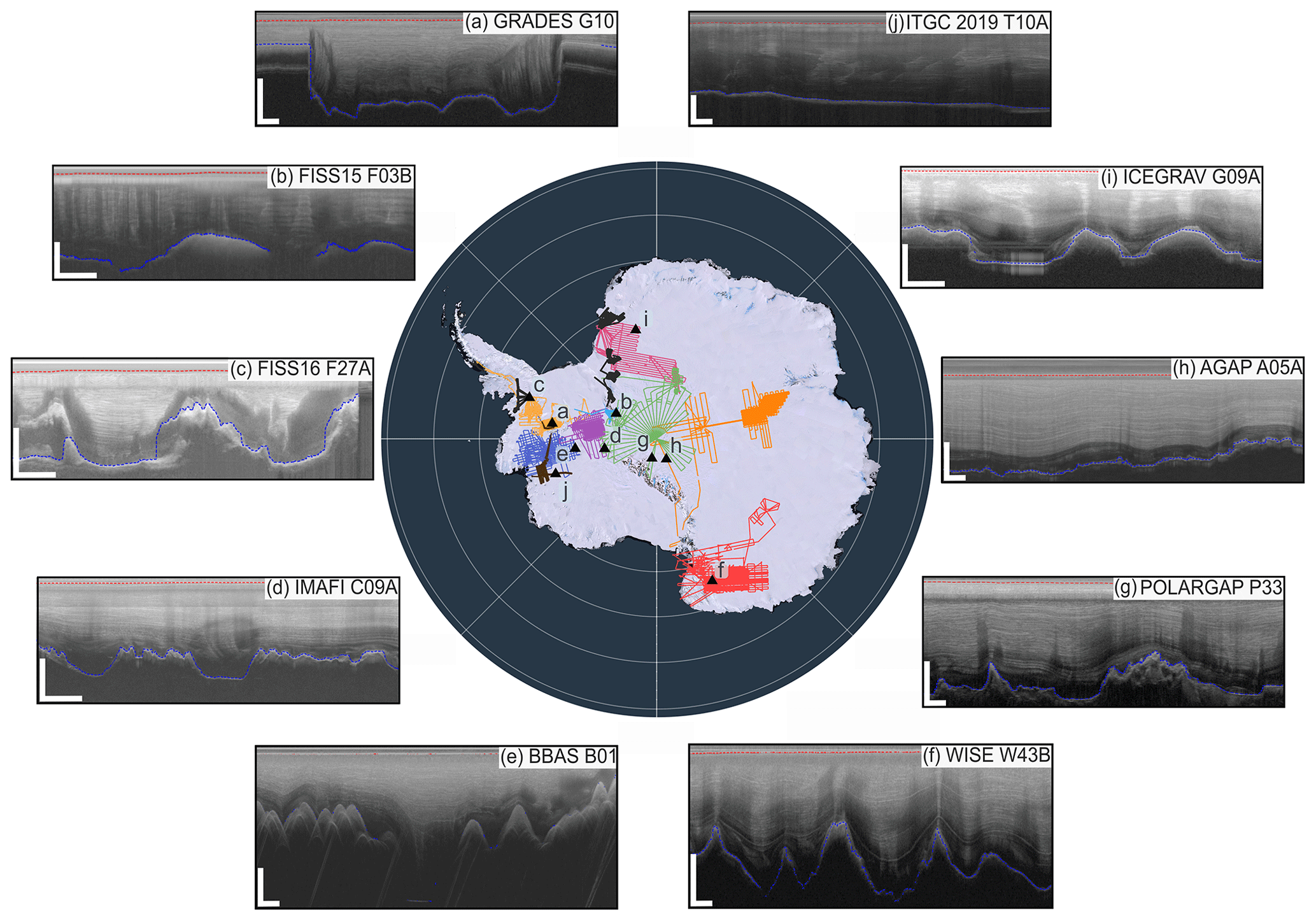
Figure 3 Sample radargrams from the 10 2-D radar datasets released with this paper. The colours for each survey on the map are the same as in Fig. 1 and the data portal. The location of each radargram (a–j) is marked on the map by black triangles. The dashed red and blue lines on the radargrams are the surface and bed picks, respectively. A description of each radargram is provided as follows: (a) flight line G10 (GRADES-IMAGE) showing well-defined subglacial valleys through which Evans Ice Stream flows (ice flow is approximately out of page), with stable layering present before and in the middle of the topographic low; (b) flight line F03B (FISS 2015) showing undulating bed topography and disrupted layering at the onset of Foundation Ice Stream; (c) flight line F27A (FISS 2016) showing variations in subglacial topography at the divide between the Antarctic Peninsula and West Antarctica, with potential evidence of basal freeze-on at the start of the segment; (d) flight line C09A (IMAFI) showing evidence of preserved layering despite changes in local topography at the bottleneck between East and West Antarctica; (e) flight line B01 (BBAS) over Ellsworth Subglacial Mountains showing a ∼ 1.5 km trough in the ice-sheet bed and one of the deepest points in the PIG basin with ∼ 3 km of ice underlying the surface; (f) flight line W43B (WISE-ISODYN) showing internal layers draping over the highs and lows in the local Wilkes Subglacial Basin topography, with two particularly bright reflections in the middle and bottom of the ice column; (g) flight line P33 (PolarGAP) showing clear and stable englacial layering throughout the ice column at the onset of the topographic highs of the Transantarctic Mountain Range; (h) flight line A05A (AGAP) showing stable internal layering characteristic of the interior of the EAIS; (i) flight line G09A (ICEGRAV) showing evidence of a bright reflection likely associated with a previously unidentified subglacial lake in the region; and (j) flight line T10A (ITGC 2019) showing a section of inland-sloping bed from a profile in the main trunk of Thwaites Glacier, > 200 km from the current grounding line position (ice flow is right to left). The horizontal and vertical white bars at the bottom of each radargram represent ∼ 3 km in the horizontal direction (i.e. distance) and ∼ 1 km in the vertical direction (i.e. depth), respectively.

3 Data acquisition and processing

The typical acquisition and processing workflow for the aerogeophysical data is shown in Fig. 4. Usually, the aircraft is set up systematically to acquire gravity, magnetic, and radar data together, except in situations where surveying objectives are not compatible with the acquisition of all three datasets at once (i.e. flying at constant terrain clearance for the radar data affects the quality of the gravity data which is better flown at constant altitude, and vice versa); although novel gravity-acquisition methods are increasingly making this issue redundant (see Sect. 3.1.1). As shown in Table 1, the conventional gravity–magnetic–radar set-up was used in 15 out of 24 surveys, with the remaining 7 surveys using either a magnetic–radar- or gravity–magnetic-only set-up, and only 2 using a magnetic-only set-up. The data acquisition steps for each type of data are described in Sect. 3.1, and the processing of the data is described in Sect. 3.2.

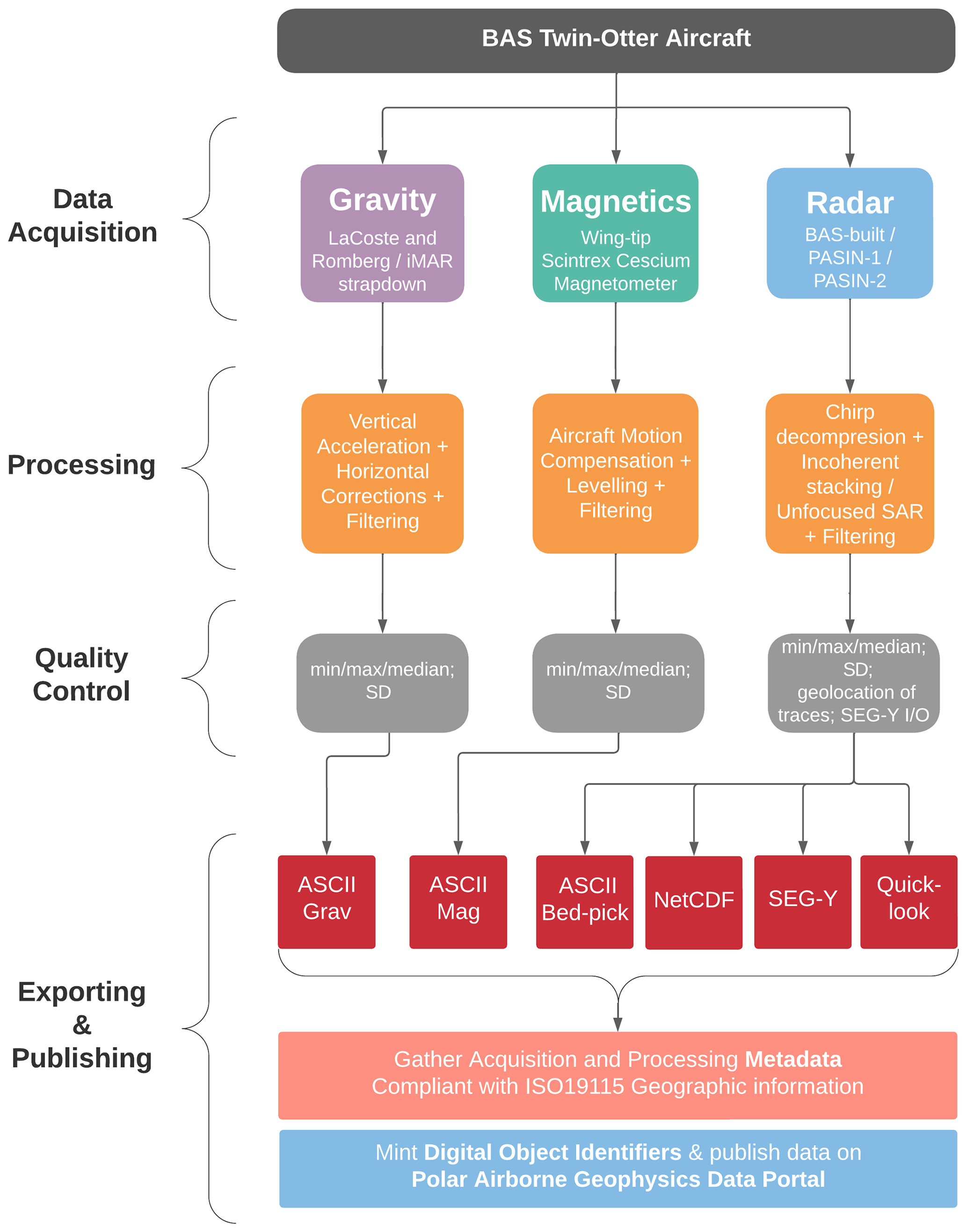
Figure 4 Workflow describing the data acquisition, processing, and publishing for the BAS aerogeophysical data included in this data release. Standard deviation is abbreviated as “SD”, whilst “I/O” refers to the import of the SEG-Y files into seismic-interpretation software for quality check and the output of the files.

3.1 Data acquisition and instrumentation

All BAS aerogeophysical data acquisition is conducted using Twin Otter aircraft due to their remote capabilities, long fuel range (up to 1000 km), and operability. The aircraft's twin turbo-prop engines enable it to conduct rapid take-off and landing as well as operate in small and remote airfields commonly covered in snow and icy terrains using mounted skis. All data acquisition since the early 1990s has been conducted using the BAS DeHavilland Twin Otter aircraft “VP-FBL” (Fig. 5). The aircraft typically flies at a nominal speed of ∼ 60 m s⁻¹, which results in an along-track distance between each stacked radar trace of 0.2 m (prior to processing). The following sections describe the acquisition of the data for the gravity (Sect. 3.1.1), magnetic (Sect. 3.1.2), radar (Sect. 3.1.3), and GPS and lidar (Sect. 3.1.4) instruments on board the aircraft.

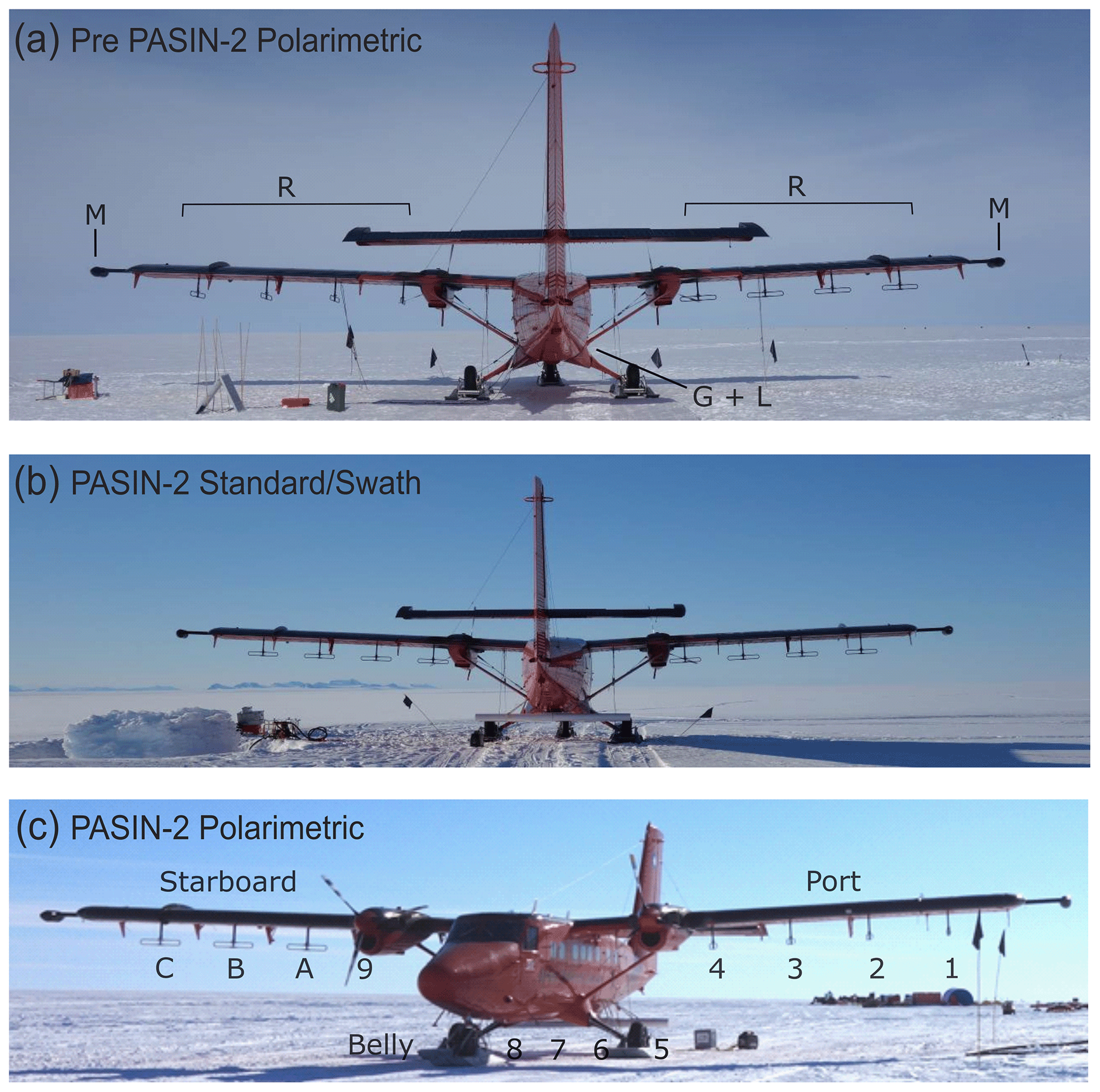
Figure 5 Photographs of the aerogeophysical set-up on the BAS Twin Otter aircraft “VP-FBL” for PASIN-2. (a) The pre-PASIN-2 (used in 2015–2016 PolarGAP only) configured to mimic the set-up of PASIN-1 data collection in polarimetric mode. The eight folded dipole transmitting and receiving antennas are fixed under the wings (two transmitting and two receiving antennas on each wing) with the port configured as vertical (V) and starboard as horizontal (H). The annotations show the location of the radar (R), magnetic (M), and gravity and lidar (G + L) instruments on board the aircraft. (b) The PASIN-2 set-up in standard/swath mode. The eight folded dipole transmitting and receiving antennas are fixed under the wings and inside the aircraft and are operated using a radio frequency (RF) switch, and an additional four receiving antennas are situated in the belly enclosure. When in standard swath mode, all antennas are configured in H orientation with the starboard and belly antennas also in H orientation. The PASIN-1 set-up in standard mode (not shown here) had a similar configuration as shown in (b) bar the belly antenna (i.e. only four transmitting on port and four receiving on starboard in H orientation). (c) The PASIN-2 set-up in polarimetric mode. The eight folded dipole transmitting and receiving antennas are fixed under the wings and inside the aircraft and are operated using an RF switch, and an additional four receiving antennas are situated in the belly enclosure. When in polarimetric mode, the port antennas are configured in V orientation and the starboard and belly antennas in H orientation. The PASIN-1 set-up in polarimetric mode (not shown here as rarely flown) had the two pairs of outboard antennas rotated to V configuration and the inboard to H configuration. Photo credit: Carl Robinson.

3.1.1 Gravity

Until 2012, BAS aerogravity measurements were acquired with a LaCoste and Romberg air–sea gravimeter modified by Zero-Length Spring (ZLS) Corporation. The gravimeter was mounted in a gyro-stabilized, shock-mounted platform at the centre of the aircraft to minimize the effect of vibrations and rotational motions.

Starting with the 2015–2016 PolarGAP survey, aerogravity data were acquired using a novel strap-down method which, unlike traditional surveys using a stabilized gravity platform, allowed for the collection of gravity data during draped or turbulent flights (Jordan and Becker, 2018). For this survey, both the LaCoste and Romberg and strap-down systems were operated, together with results from the two systems merged, to provide an optimum data product with the long-term low and predictable drift of the LaCoste and Romberg system and the dynamic stability of the strap-down system. Subsequent surveys used a strap-down sensor alone, removing the need to prioritize the quality of the gravity data over the radar data and allowing for flights at a constant terrain clearance for optimal radar-data collection. The optimum resolution of the system is approximately 100 s along-track (Jordan and Becker, 2018).

The first strap-down sensor deployed by BAS was the iMAR RQH-1003 system provided by the Technical University (TU) of Darmstadt, and consisting of three Honeywell QA2000 accelerometers (mounted in mutually perpendicular directions) and three Honeywell GG1230 ring laser gyroscopes. The subsequent 2018–2019 and 2019–3020 ITGC surveys over Thwaites Glacier used the iMAR iCORUS strap-down airborne gravimeter systems from Lamont-Doherty Earth Observatory and BAS respectively, which have approximately equivalent internal components to the TU Darmstadt system.

3.1.2 Magnetics

The Twin Otter is configured for fixed wing magnetometer operation. The aircraft modifications include inboard-positioned wingtip fuel pumps, pod-boom hard points and a demagnetized airframe to maximize magnetic-data collection. Scintrex CS3 Cesium sensors are used due to their high sensitivity, high cycling rates, excellent gradient tolerance, fast response, and low susceptibility to the electromagnetic interference. The resolution of the magnetometers has greatly increased over time, with the current systems having a measurement accuracy of 0.2 pT compared to the older systems used between 1973 and 1990 (500 pT; Geometrics G-803 Potassium) and between 1991 and 2003 (10 pT; Sintrex H8 Cesium).

3.1.3 Radar

Prior to 2004, BAS deployed a custom-built, 8-array element radar system, referred to here as “BAS-built” (Corr and Popple, 1994). This was a coherent radar system operating at a centre frequency of 150 MHz and using a transmit power of 1200 W (Rippin et al., 2003a). The radar system was equipped with eight folded dipole transmitting and receiving antennas fixed under the wings (four transmitting on the port wing, four receiving on the starboard wing). Similar to the current systems, the “BAS-built” system transmitted both a conventional narrow-sounding pulse mode of 0.25 µs and a deep-sounding 4 µs, 10 MHz chirp (Table 2). As developments in digital acquisition became commercially available, several technical upgrades were applied to the radar system. These ranged from using a LeCroy scope to acquire logarithmic detected waveforms to accommodate complex coherent acquisition, as well as the replacement of the LeCroy oscilloscope by a low sample-frequency 12 bit dual ADC (analogue-to-digital converted) card in the later years of operation (see Fig. S1 in the Supplement). During this time, the dynamic range of the system was extended by the interleaved transmission of different waveforms, which were conventional short wave-train pulses at the centre frequency.

After operating for 10 successive field seasons, the “BAS-built” radar system was retired and was replaced by a more modern radar system, PASIN (Corr et al., 2007). In contrast to the “BAS-built” system, PASIN was designed to sound ice much deeper (up to 5 km compared to 3.3 km for the earlier system) thanks to improved digital electronics and added power in the transmitting antennas (see Table 2). Additionally, modern methods of digitization, enabled by the use of ADC cards rather than a digitizing scope, allowed phase and not just power to be recorded in greater resolution on PASIN, which eventually allowed for the use of more advanced processing techniques such as synthetic aperture radar (SAR) to be applied to the data (see Sect. 3.2.3).

The older PASIN-1 (2004–2015) and the newer PASIN-2 (2015–present) systems are bistatic radars operating at a 150 MHz centre frequency and configured as follows: (a) PASIN-1: 10 MHz bandwidth system with eight folded dipole transmitting and receiving antennas fixed under the wings (four transmitting on port wing, four receiving on starboard wing) operating in horizontal (H) orientation when in standard mode, and more rarely with the port (transmit) and starboard (receive) antennas positioned in both H and vertical (V) orientation when in polarimetric mode (see similar set-up of PASIN-2 in Fig. 5a) (Corr et al., 2007); and (b) PASIN-2: 13 MHz bandwidth system with eight folded dipole transmitting and receiving antennas fixed under the wings and inside the aircraft with radio frequency (RF) switches and an additional four receiving antennas in the belly enclosure (see Fig. 5b–c; Table 2). The main difference between the PASIN-1 and PASIN-2 systems is the ability for across-track swath processing to be applied to the PASIN-2 data by allowing both transmitting and receiving on the folded dipole antennas via the use of RF switches.

In further contrast with PASIN-1, the PASIN-2 radar has a very flexible configuration, with the standard configuration being as 12-channel swath radar (with 8 transmitting and 12 receiving). However, other configurations are also possible, including a polarimetric mode to give H and V data where the port antennas are rotated 180^∘ (see Table S1 in the Supplement). A final configuration is a mixed antenna gain path for areas where ice is heavily disrupted and where the starboard signal can be attenuated by several decibels. Since 2016, the PASIN-2 system has undergone minor modifications to reduce noise and improve system operations, including (a) low-pass filters in the RF switches, (b) the use of a 10 GHz waveform generator, and (c) new 1 kW solid-state power amplifiers which have lowered transmitter system noise and increased transmitter and receiver isolation.

Data for both versions of the PASIN system are received using sub-Nyquist digitization and stacking and stored on removable solid-state disks or tapes, and then copied to duplicate spinning disks for data archiving. On average, a 4.5 h flight will generate ∼ 150–200 GB of data for PASIN-1 and up to 3 TB of data for PASIN-2. The systems systematically acquire a shallow-sounding 0.1 µs pulse (PASIN-1)/1 µs short-attenuated chirp (PASIN-2), and a deep-sounding 4 µs, 10 MHz (PASIN-1)/13 MHz (PASIN-2) linear chirp (Table 2). The shallow-sounding pulse/short-attenuated chirp product is best used to assess internal layering in the upper ∼ 1.5–2 km of the ice sheet, whereas the deeper-sounding chirp is best suited to assess englacial layering and bed characteristics in deep-ice conditions (Fig. 6c–e). The radar is capable of sounding ice to depths of up to 5 km with a horizontal resolution of 10 cm (before processing) and a depth resolution in the vertical direction of 8.4 m (PASIN-1) and 6.5 m (PASIN-2).

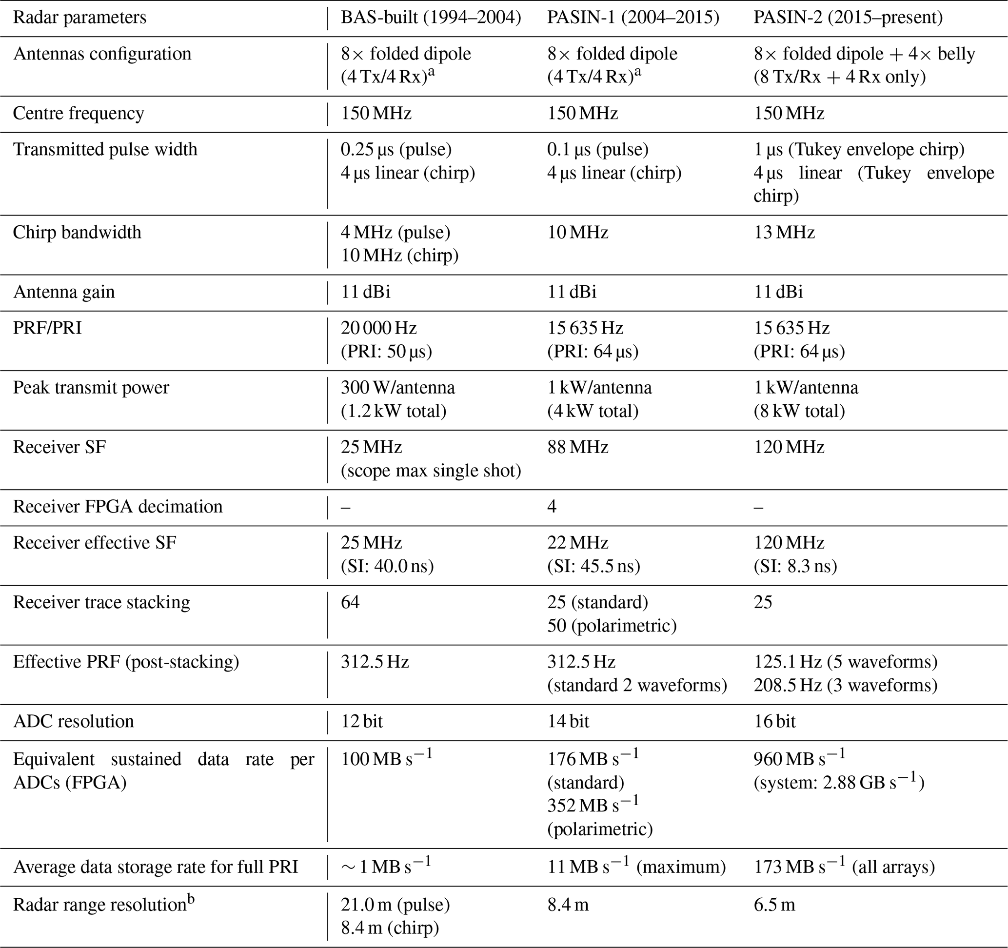
Table 2 Radar parameters for the three radar systems deployed by BAS between 1994 and the present day. Note that PASIN-1/2 have a number of programmable settings for flight-specific objectives (e.g. one to eight waveforms programmable for PASIN-2), and the numbers provided here are for the most commonly used settings. For PASIN-2, a standard set-up consists of five waveforms as follows: 4 µs H (0^∘), 4 µs V (0^∘), 4 µs H (90^∘), 4 µs V (90^∘), 1 µs H (Table S1). Abbreviations in the table are as follows. ADC: analogue-to-digital converter; FPGA: field-programmable gate array; SF: sample frequency; SI: sample interval; PRF: pulse-repetition frequency; PRI: pulse-repetition interval. ^a BAS-built and PASIN-1 systems used RF combiners on the receiver to produce a single RF input-to-sample, with PASIN-1 splitting these into a high- and low-gain channel for standard mode (two ADC channels) and combining these for pairs of H and V in polarimetric mode (four ADC channels). ^b Radar Range Resolution is calculated using a radio-wave velocity in ice of 168 m µs⁻¹ and does not include the effect of the processing on the vertical resolution of the system, which is expected to be ∼ 50 % greater than the values provided in the table, thus these numbers should be interpreted as the theoretical system performance. Diagrams showing the configurations of the three radar systems are provided in the Supplement (Figs. S1–S3).

The pulse repetition frequency of the PASIN ($\mathrm{1}/\mathrm{2}$) system is 15 635 Hz and hardware stacking is typically set to 25 in standard mode, which results in an effective pulse-coded waveform acquisition rate of 312.5 Hz for each transmit pulse (Table 2). Following stacking, the final sampling frequency of PASIN-1 is 22 MHz and PASIN-2 is 120 MHz (Table 2).

3.1.4 GPS and lidar

Since 1978, navigation has transitioned from basic aircraft data, imagery, and dead reckoning to more modern means, including the use of the carrier-phase Global Positioning Systems (GPS).

Between 1994 and 2004, the BAS Twin Otter aircraft was equipped with a Trimble GPS system (1994–1995 surveys: Trimble 4000SSE; 1996–2003 surveys: Trimble 4000SSI). Since 2004, the aircraft is equipped with two, 10 Hz GPS receivers (Leica 500 and ASHTEC Z12 for 2004–2018 surveys; Javad Delta and Novatel Span for post-2018 surveys) installed on board the aircraft. On the ground, two Leica 500 GPS base stations (replaced by Javad TRIUMPH-2 for post-2018 surveys) are positioned and equipped with choke-ring antennas, set up specifically to obtain an unobstructed view of the sky above. Aircraft turns are typically limited to 10^∘ banking angles in order to avoid losing lock with GNSS satellites orbiting close to the horizon. The estimated accuracy of the absolute position of the aircraft is 10 cm or less, with the relative accuracy approximately 1 order of magnitude better. Since 2010, the aircraft altitude and inertial information has been provided by an iMAR FSAS inertial measurement unit (IMU), with the data logged on a Novatel Span receiver. Additional altitude information from the strap-down gravity system is also available for post processing of other datasets.

For all modern surveys, the aircraft was also equipped with a Riegl Q240i-80 laser altimeter system (or lidar) in the floor camera hatch to accurately detect the ice surface. The lidar data used for correction of the radar data are typically extracted from the nadir point value with no correction for aircraft altitude. The system has a repetition frequency up to 2 kHz which results in an along-track measurement every 3 cm with an accuracy of up to 5 cm. The lidar is used up to altitudes of 700 m and is constrained by cloud-/fog-free conditions. From 2010 onwards, the lidar onboard the Twin Otter was capable of obtaining swath lidar data, although only the single-point data along the centre line were provided as part of this data release.

3.2 Data processing

3.2.1 Gravity

The raw aerogravity data are processed to obtain levelled free-air gravity anomalies. Although additional survey-specific processing might have been applied to the data, general processing steps for the LaCoste and Romberg system include the calculation of the observed gravity and a range of corrections and filtering functions as described in Jordan et al. (2007, 2010) and Valliant (1992). In particular, corrections for vertical acceleration, Eotvos horizontal motion (Harlan, 1968), latitude (Moritz, 1980), and free air (Hackney and Featherstone, 2003) were applied to obtain the final free-air anomalies before subsequent 9–12 km low-pass filtering. As the free-air values refer to the WGS84 ellipsoid, they are defined in geodesy as gravity disturbance (Hackney and Featherstone, 2003).

The strap-down gravity method adopted from 2015 onwards directly combined observations of acceleration in all three axes, with orientation and GPS observations combined in a Kalman filter to simultaneously solve for aircraft position and variations in the Earth's gravitational field (Becker et al., 2015). For subsequent strap-down-acquisition surveys, some amount of thermal drift levelling/correction is required. Spectral analysis suggests that the strap-down system can resolve wavelengths on the order of ∼ 5 km (Jordan et al., 2020). Error estimates for the gravity data can be found in the respective survey metadata (see Table 3), or in specific studies utilizing the BAS aerogravity data (e.g. Ferraccioli et al., 2006; Forsberg et al., 2018; Jordan and Becker, 2018).

Additional processing may include the use of masks to remove aircraft turns, start and end of lines, and other regions of noisy data, or producing an upward continued free-air anomaly by the upward continuation of each line segment from the collected flight altitude to the highest altitude in the survey. The first level of free-air anomaly for all published BAS data is shown in Fig. 2a, although it is worth noting that no correction such as downward continuation has been applied to compile the data shown in Fig. 2a. It is considered that at the scale of the map, the vertical gradient of residual gravity anomalies at flight altitude is inferior to 2 mGal. Additionally, as the gravity surveys are acquired over the ice sheet, the distance to the bedrock is not only dependent on the flight altitude but also on the ice thickness.

3.2.2 Magnetics

The raw aeromagnetic data have been processed using the SCAR ADMAP2 data-release protocols (Golynsky et al., 2018). Data were collected at 10 Hz, allowing for modelling and removal of aircraft dynamic movements using a so-called compensation correction (Ferraccioli et al., 2007). This correction typically requires a dedicated calibration flight in the direction of the survey lines and tie-lines to have been flown. For some surveys with radial design, or where magnetic-data acquisition was opportunistic, logistical constraints meant no calibration flight could be conducted. In these cases, the generally large depth-to-source estimates due to the thick ice allowed for a 10–15 s filter to be applied to minimize noise generated by aircraft motion without compromising the geological signal. Given the redundancy of collecting 10 Hz (∼ 6 m spaced) observations over thick ice, most surveys were downsampled to 1 Hz (∼ 60 m) prior to further processing.

After magnetic compensation, the magnetic data were corrected for the International Geomagnetic Reference Field (IGRF), which is a standard mathematical description of the Earth's main magnetic field. Data impacted by operation of aircraft systems such as pumps and heaters were manually determined. Typically, such data were discarded, but survey design and lack of alternative data sources mean that sometimes important geophysical signatures may be present. In some cases, the contaminated data were therefore corrected using an offset correction, accepting that the data segment may be more noisy.

Magnetic data were then corrected for diurnal variations in the magnetic field using observations at a fixed base station, typically filtered with a 30 min filter to remove short-wavelength noise potentially not seen on the aircraft. Further statistical levelling of the data based on internal intersections and crossovers with previous surveys was carried out at times to remove systematic errors associated with flight direction (i.e. heading corrections) and additional long-wavelength errors associated with incomplete removal of diurnal variations. In some cases, continuation to a fixed altitude above the ice-sheet bed and a final grid-based micro-levelling procedure were applied (Ferraccioli et al., 1998). The magnetic anomaly map shown in Fig. 2b shows the spatial coverage and magnitude of magnetic data available. Errors in the data are typically presented as the standard deviation of the crossover errors and can be found in the respective survey metadata (see Table 3).

3.2.3 Radar

All data acquired with the earlier “BAS-built” radar system (1994–2004) were read using C code software to convert the LeCroy data to formats readable by Halliburton Landmark's seismic-processing software, SeisSpace ProMAX (hereafter referred to as ProMAX). Basic processing was applied to the data in the hardware analogue domain and later using ProMAX, including power normalization and final SEG-Y export. Following the transition from the LeCroy oscilloscope to ADC cards on the “BAS-built” system (see Sect. 3.1.3), MATLAB replaced the IDL language for data processing.

As opposed to the “BAS-built” system which, by design, had some level of processing done on the raw data internally, the PASIN system was designed to retain much of the sampled data in the rawest form possible to allow for evolving processing techniques to be applied to the data in the future. For all PASIN data (2004 onwards), the first high-level step was to extract the raw data from the tape drives, convert the 3-byte values to conventional 4-byte integers, combine the waveforms associated with each pulse transmit type, and then export the data into MATLAB-formatted binary files. The second high-level step was to minimize side-lobe levels by applying a chirp-decompression technique using a Blackman window from a custom-built MATLAB toolbox, resulting in a processing gain of ∼ 10 decibels (dB).

The next step was to apply processing techniques both to enhance along-track resolution and improve the signal-to-noise ratio. For the 2004–2005 BBAS survey, incoherent stacking of 10 consecutive traces was applied and a moving-average window filter used; however, no SAR techniques were initially applied to these data. First tested on previously acquired PASIN radar data (see Hélière et al., 2007), 2-D SAR processing based on the Omega-K algorithm and subsequently improved versions using Doppler-beam sharpening were applied systematically to all the deep-sounding chirp data from 2005–2006 onwards to increase spatial resolution and remove backscattering hyperbolae in the along-track direction (Corr et al., 2007; Jeofry et al., 2018). The benefit of using unfocused along-track SAR processing is that it resolves the bed in much finer detail compared with non-SAR focused data (see Fig. 6d–e). However, SAR-processing can also lead to distortions of the amplitude of the ice structure and bed reflection in inhomogeneous areas of the ice sheet (e.g. near the grounding line; see Hélière et al., 2007) and thus might not always be appropriate for assessing internal layering or absolute amplitudes such as required for bed-reflectivity analysis (e.g. Peters et al., 2007; Castelletti et al., 2019). Additional moving-average filters of varying lengths have also been applied to enhance englacial reflections and improve visualization of the radar data.

Figure 6 shows the three processed radar products provided for the 2010–2011 IMAFI survey over West Antarctica. Figure 6c shows the shallow-sounding pulse and Fig. 6d–e the deep-sounding chirp radar data using the unfocused SAR-processing technique from Hélière et al. (2007) (Fig. 6d) and a version of the chirp product processed with coherent summations but with no SAR-processing applied (Fig. 6e). Internal layering is more clearly visible in the upper part of the ice column on the pulse data compared with the chirp data (see black-bordered insets in Fig. 6c and e). In contrast, deeper internal layering is much more visible on the SAR-chirp than on the non-SAR chirp (Fig. 6d–e). Additionally, the peak amplitude of the bed is better resolved in the SAR-processed chirp than in the non SAR-processed chirp (see white-bordered inset in Fig. 6d–e).

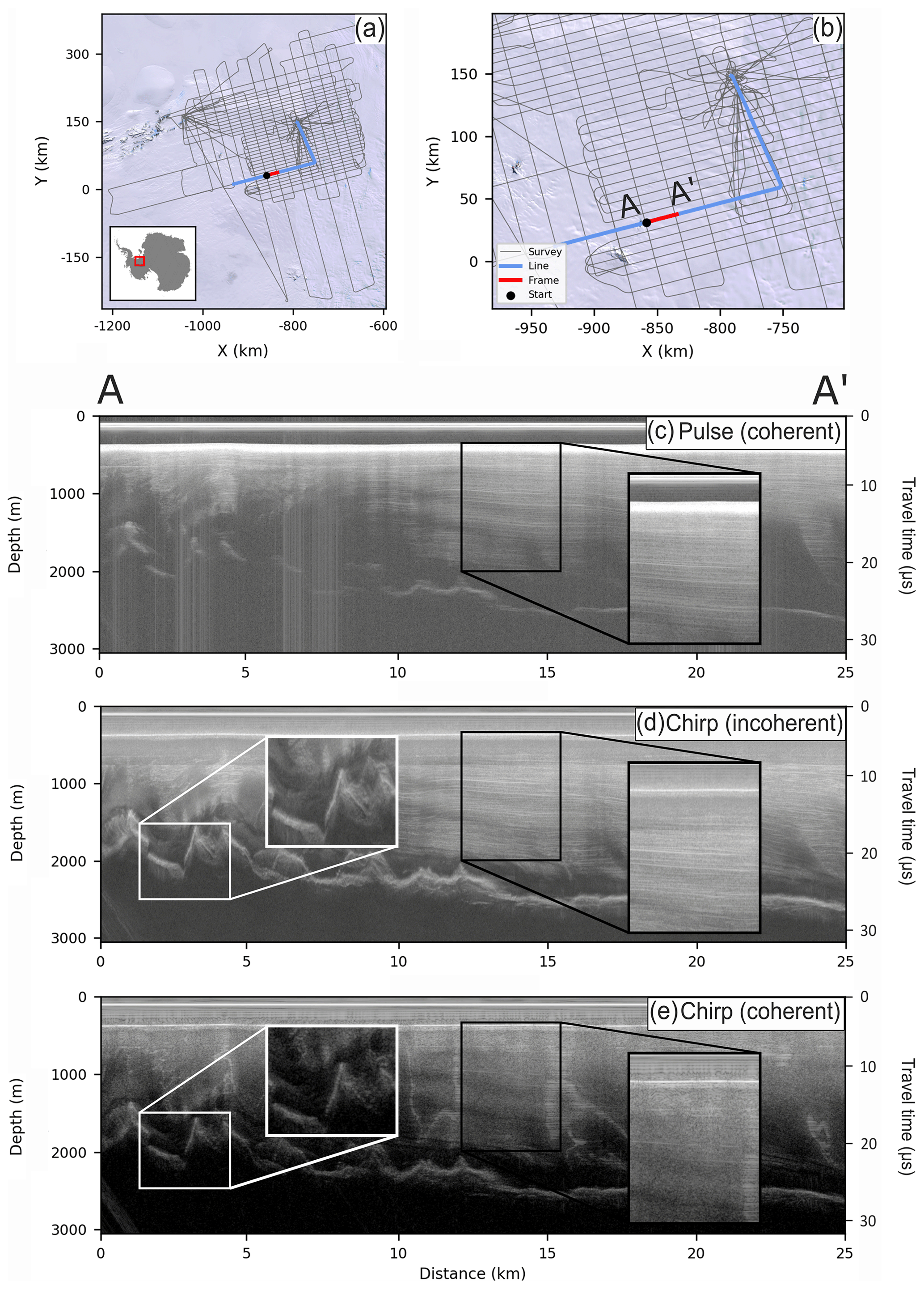
Figure 6 A 25 km segment of flight line 15d of the 2010–2011 IMAFI survey, showing the three radar products and processing attributes: (a) shows an overview map of the entire survey with an inset over Antarctica, and (b) shows a zoomed-in map over the specific flight line with the 25 km radar segment (defined as A–A^′) shown in red. The background satellite image in (a)–(b) is from the Landsat Image Mosaic of Antarctica (LIMA) (Bindschadler et al., 2008). Images (c)–(e) show a 25 km segment of the data for the three products provided for the 2010–2011 IMAFI survey as follows: (c) the coherently processed, shallow-sounding pulse, (d) the unfocused 2-D SAR-processed, deep-sounding chirp, and (e) the coherently processed, deep-sounding chirp. The black-bordered insets zoom to the internal layering in the upper portion of the ice column for (c)–(e) and the white-bordered insets show the difference in bed characteristics between (d) and (e).

Further processing of the PASIN data has also been applied by others using simple image-processing techniques such as moving-average filters to enhance the internal layering of the ice and reduce incoherent noise (Ashmore et al., 2020; Bodart et al., 2021) or by applying more complex SAR-processing techniques over previously incoherently processed radar data (Castelletti et al., 2019; Chu et al., 2021). Additional techniques have also been employed in areas where side echoes from steep valley walls lead to ambiguous bed reflections, as previously employed over Flask Glacier (Antarctic Peninsula) using PASIN SAR-processed data and a combination of velocity and digital elevation models to obtain more accurate ice-thickness estimates (Farinotti et al., 2013).

Following radar data processing, bed and ice-surface reflections were determined by picking the onset of the basal echo (i.e. where the echo amplitude is greater than the noise floor). We note that this is not a universal method applied by all radar data providers, who may pick the half-amplitude delay or the peak value, leading in turn to measurement biases across data providers and products (e.g. Peters et al., 2005; Chu et al., 2021).

The BAS approach to picking the bed was to use a semi-automatic first-break pick algorithm on the chirp data below a top-mute window in ProMAX (generally ∼ 100 samples above the approximate bed reflection) to locate the precise bed return, followed by manual checks and re-picking to exclude any unrealistic spikes. In areas where multiple closely spaced reflections were sounded at the bed, the shallowest reflection was assumed to be the bed as off-axis reflections would likely appear lower down in this section. However, in some cases, deeper reflections were chosen, with shallower weak reflections assumed to reflect entrained debris, accreted ice, or uncompensated refraction hyperbolae close to the bed. We note, however, that this method has evolved over the years, and that its success is inherently reliant on the radio-glaciological experience of the human picker to quality-check the results from the semi-automatic picker and manually re-pick the data if necessary. The uncertainty associated with the picking procedure can be partially approximated by calculating the root mean square error (RMSE) of the bed elevations at crossover points across the survey area. Although these errors are site-specific and can depend on factors such as varying bed topography and roughness, larger errors may reflect uncertainties in data processing or analysis (i.e. picking in this case). Areas of more extreme topography typically show the highest crossover errors, likely associated with off-axis reflections and entrained debris close to subglacial cliffs, which make deciding on the correct bed pick challenging. In isolated cases, such errors can exceed several hundred metres. In contrast, regions dominated by smooth and flat beds typically show lower crossover errors, on the order of several metres only. Survey-wide RMSEs are typically reported in each survey's metadata (see Table 3) and average ∼ 9–22 m depending on the survey (see Rippin et al., 2003a; Vaughan et al., 2006; Ross et al., 2012; Jeofry et al., 2018).

To estimate ice thickness and hence obtain the bed elevation, the location of the surface reflection in the radar data must be known accurately. However, since the PASIN system does not resolve the ice surface well due to errors in the phase centre of the pulse through the firn layer, the surface reflection in the radargram was only rarely used on its own to calculate the ice surface. Usually, range-to-surface from coincident on board-acquired lidar, or alternatively, if lidar was not available (i.e. due to clouds or ground clearance higher than 750 m), using the aircraft's radar altimeter or surface elevation from an accurate digital elevation model (DEM) (i.e. REMA 8 m DEM for latest surveys; Howat et al., 2019), was used to calculate a “theoretical” surface pick, as follows:

Firstly, the same semi-automatic picker used for picking the bed was used on a subset of the shallow-sounding pulse radargrams with a bottom-mute window set at ∼ 100 samples below the surface reflection. Secondly, once aircraft-to-surface range was obtained from lidar, a linear trend between the surface pick from the radargram and the surface range from the lidar was calculated, and a resulting slope and offset was used to calculate the theoretical location of the surface. Where possible, the range-to-ground value was derived from the lidar data or interpolated from the mean lidar elevation within ∼ 700 m. In those rare cases where the surface reflection was picked directly from the radargram, a regression, local to the data gap, was used to fit the radar range-to-terrain clearance. If lidar was not available to calculate range-to-ground, the height of the aircraft above the surface was obtained by the aircraft's radar altimeter which was then converted into a radar delay time. This conversion was done after a two-stage calibration process which involved recording the terrain clearance over a sea surface with the two instruments, and then correction for the penetration depth of the radar altimeter was obtained from the difference in the height above ellipsoid for a surveyed “flat” snow surface and the aircraft. Where possible, the reference surface was chosen to be in the centre of the targeted area.

Once bed and surface were calculated, ice thickness was obtained by calculating the difference between the bed and surface pick in range samples (relative to the BAS system). The picked travel time was then converted to depth in metres using a radar wave speed of 168 m µs⁻¹ and a constant firn correction of 10 m. Bed and surface elevations were then integrated with a high-precision kinematic dual-frequency GPS position solution to provide the final point dataset of elevations relative to the WGS84 ellipsoid. To ensure the best accuracy of satellite-orbit definitions and atmospheric corrections, the interpolated survey locations and aircraft elevations were processed from 10 Hz coupled Precise Point Positioning (PPP) GNSS/INS solutions 1 month after data acquisition.

4 FAIR data publishing

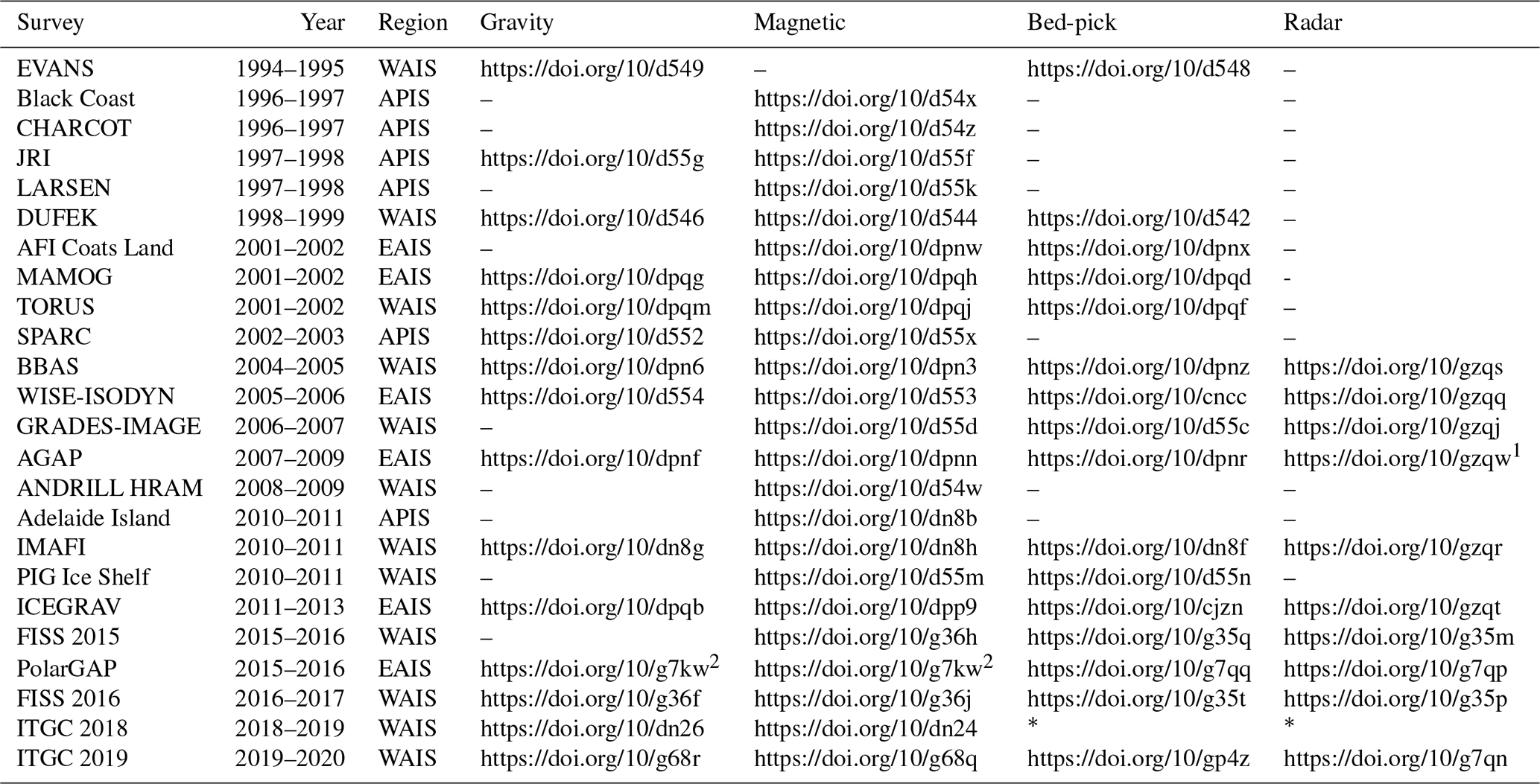
In total, we have published 64 datasets from 24 surveys as part of this data release, representing ∼ 566 GB of data and ∼ 1800 files. This amounts to a total of 3.62 million gravity and 7.41 million magnetic data points, as well as 14.5 million ice-thickness and bed-elevation measurements. The complete list of published datasets is provided in Table 3, including the short digital object identifiers (DOIs), which redirect to the metadata sheets and download folders for each respective dataset archived on the PDC Discovery Metadata System (DMS) data catalogue (https://data.bas.ac.uk/, last access: 18 July 2022).

Table 3 Short digital object identifiers (DOIs) for the gravity, magnetic, bed-pick, and 2-D radar datasets of each survey flown by BAS and included in this data release. Abbreviations used are the same as in Table 1. ¹ For the AGAP radar data, the US-led survey lines can be found at https://doi.org/10.1594/IEDA/313685 (Bell, 2011). ² For the PolarGAP survey, data can be downloaded from both the ESA and BAS data catalogues, but the DOI for the gravity and magnetic data (https://doi.org/10.5270/esa-8ffoo3e, Forsberg et al., 2017) belongs to ESA. If using the PDC data catalogue, the PolarGAP gravity and magnetic data can be downloaded from https://data.bas.ac.uk/full-record.php?id=GB/NERC/BAS/PDC/01583 (last access: 18 July 2022) and https://data.bas.ac.uk/full-record.php?id=GB/NERC/BAS/PDC/01584 (last access: 18 July 2022), respectively. “*” indicates that the data are not held at BAS, but instead are available on the CReSIS data portal (https://data.cresis.ku.edu/, last access: 18 July 2022).

We note that individual profiles acquired opportunistically following larger aerogeophysical surveys (i.e. flight lines over Flask Glacier; Farinotti et al., 2013) are not included in this data release unless specifically mentioned in the metadata for each survey (see Table 3). Such small-scale datasets will be added to the data portal in future releases (see Sect. 4.3).

Below, we discuss the release of the datasets centred around the four FAIR data principles (i.e. findable, accessible, interoperable and re-usable; Wilkinson et al., 2016), starting with the formats and attributes used to store and describe the data (Interoperability; Sect. 4.1), the metadata and DOIs assigned to each dataset (Findability; Sect. 4.2), the data-portal interface and functionalities (Accessibility; Sect. 4.3), and finally the creation of a user guide and open-access tutorials written in Python and MATLAB for reading the data programmatically (Re-usability; Sect. 4.4).

4.1 Interoperability: data formats and attributes

In order to make our data as interoperable as possible, the choice of an open format for all our datasets was a priority. We followed the best practices of the geophysics community and used common data formats and naming conventions to describe the variable names. These are detailed further here.

The gravity, magnetic, and bed-pick data are stored in open ASCII data formats, namely XYZ and CSV files, to ensure long-term access and unrestricted use of the data in the future (Fig. 4). Additionally, we followed the SCAR ADMAP2 data-release protocols (Golynsky et al., 2018) for the naming convention of the channels for the magnetic data. For the radar data, we chose to release the bed-pick data separately from the full radar data (see Fig. 4), although the full radar product contains most of the information stored in the ASCII bed-pick files. Publishing the bed-pick data separately from the radar data was a deliberate choice: it alleviates the need for users to download the full radar datasets to access light-weight tabular data, and improves the accessibility of the point data for large gridded products such as SCAR's BEDMAP (Fretwell et al., 2013) and NASA's BedMachine (Morlighem et al., 2020) projects. The bed-pick data are stored as ASCII-formatted files (namely XYZ and CSV), whereas the full radar data are stored as SEG-Y and NetCDF files, reasons for which are described below.

The SEG-Y format has been used extensively by radar scientists since the early 1980s to store radar data. This is primarily due to the lack of a radar-specific format, SEG-Y having been developed primarily to store seismic data. The advantage of using SEG-Y files is that data can be readily imported into seismic-interpretation software for data interpretation and analysis. The drawbacks of using SEG-Y, however, are numerous, making this option unsuitable for long-term data storage. These include: (1) limited space for metadata, (2) the choice of byte-information to store the radar data is subjective due to the nature of the SEG-Y format, (3) until recently, the byte stream structure which includes the geolocation of each radar trace (i.e. the X and Y positions) was restricted to integer format leading to large inaccuracies in the actual trace position, despite the use of high-resolution, sub-metre GPS data (see Sect. 3.1.4). Recognizing, however, the geophysical community's need to view and analyse the radar data in conventional data formats, we have decided to continue producing SEG-Y files for each flight line and acquisition mode (e.g. pulse and chirp). The SEG-Y files were produced using the Revision 1.0 SEG-Y format and georeferenced using the navigational position of each trace from the GPS on board the aircraft in polar stereographic (EPSG: 3031) projection. Each SEG-Y file contains the following byte-information: trace number (byte: 1–4 and 5–8), PRI-Number (byte: 9–12), Cartesian X coordinate (byte: 73–76), Cartesian Y coordinate (byte: 77–80), number of samples for each SEG-Y trace (byte: 115–116), and the sampling interval (byte: 117–118).

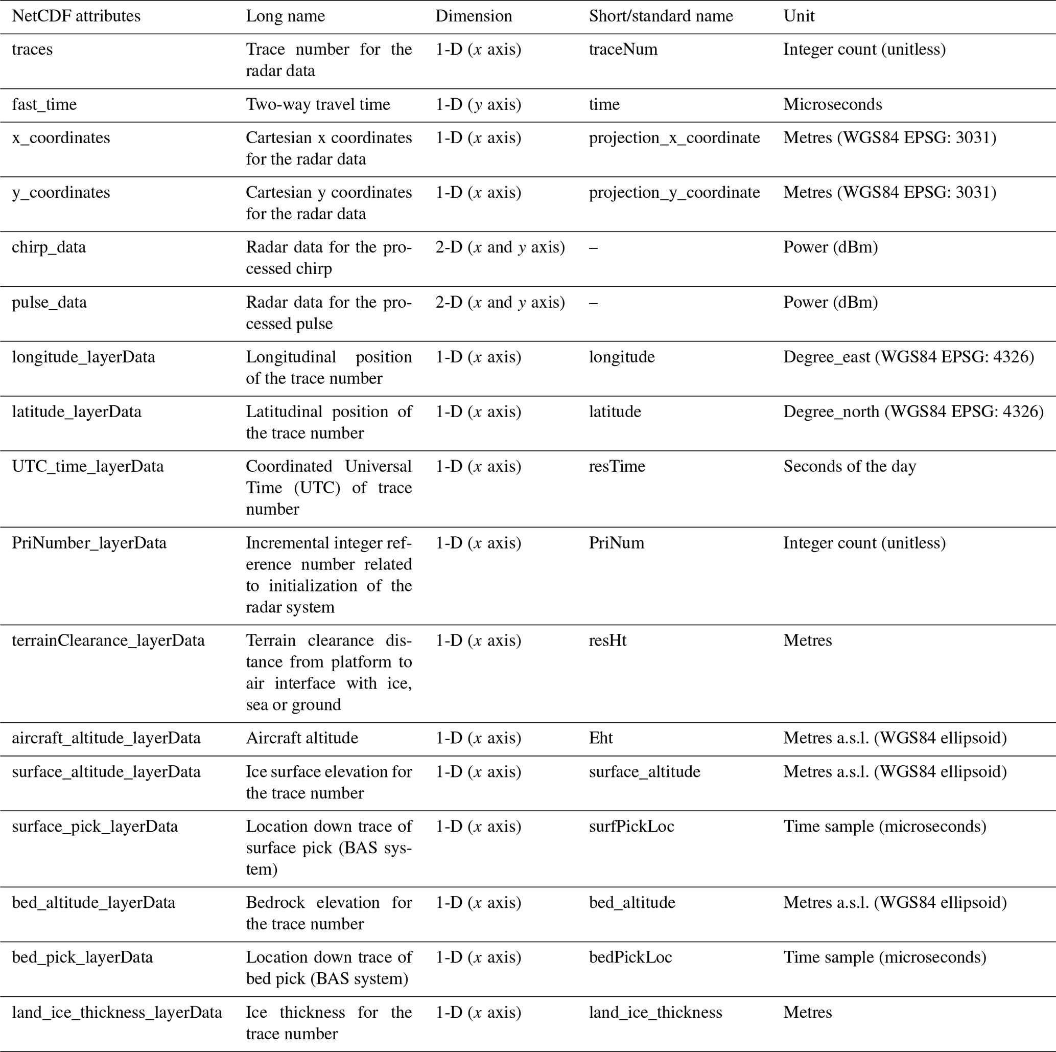
As a result of the issues mentioned above, we also exported and published the radar data in NetCDF-formatted files. We chose the NetCDF format due to its portability and array-oriented structure, the ability to store large amounts of metadata and variables into one portable file, its machine-readable capability, and to harmonize our data products with other fields such as climate science (e.g. ECMWF ERA5 reanalysis products; NCAR climate data), glaciology (e.g. Le Brocq et al., 2010; Morlighem et al., 2017; Lei et al., 2021) and, increasingly, radar geophysics itself (e.g. Paden et al., 2014; Blankenship et al., 2017), which already all make use of this data format effectively. The NetCDF files we produced contain extensive metadata relating to the acquisition and processing of the radar data, as well as a set of Climate and Forecast (CF)-compliant variables that are tied to the radar data (https://cfconventions.org/, last access: 18 July 2022) (Table 4). As a minimum, each NetCDF file contains a radar data variable (one for the pulse and/or one for the chirp, if both exist) in 2-D format, and a set of 1-D variables relating directly to the radar data, such as the trace number, PRI number, fast time, and the X and Y coordinates (Table 4). We also provided additional radar-related variables which were extracted from the radar data following processing, such as the surface and bed picks, the surface and bed elevation, the ice thickness, longitude and latitude, time of the trace, and the elevation of the aircraft (Table 4). Additional 1-D variables include the source of the surface pick (from lidar or radar) if this exists, the range between the aircraft and the ice surface, and in case the pulse- and chirp-radar variables do not have the same length, we provide two sets of variables for the trace number and PRI number.

Table 4 Attributes for each variable stored in the NetCDF files. For each attribute name, we provide the long name, the dimension (1- or 2-D, x or y axis), the short or CF-compliant standard name, and the unit of the measurement. The standard name is only provided if it exists as part of the CF convention (https://cfconventions.org/, last access: 18 July 2022), otherwise a short name is provided. The abbreviation “dBm” stands for decibel-milliwatts and “a.s.l.” stands for above sea level. Note that the surface and bed-pick data are referenced to the sampling time of the BAS radar systems across the 64 µs pulse repetition interval window, and digitized according to the receiver sampling frequency (see Table 2).

Lastly, to aid visualization and improve efficiency in navigating the datasets, we created lightweight quick-look PDF files of the radar data for each flight line of each survey (see example for the WISE-ISODYN survey in Fig. 7). The choice of ∼ 25 or ∼ 50 km length for the 2-D radargram was chosen based on clarity of the image and varies from survey to survey. The quick-look PDF files are stored alongside the SEG-Y and NetCDF files and are accessible using the links provided in Table 3.

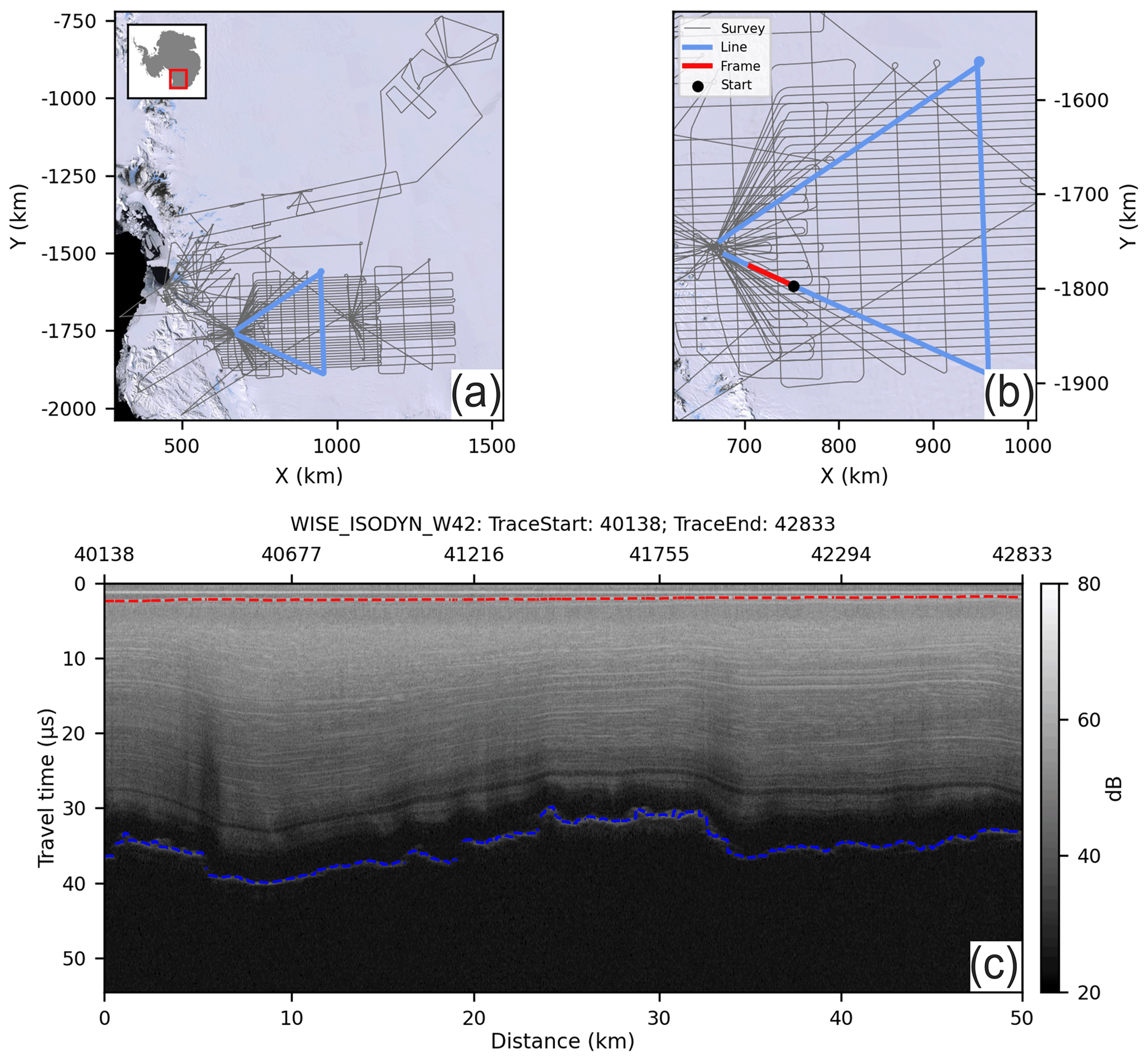
Figure 7 Example of a segmented quick-look image from the 2005–2006 WISE-ISODYN survey. (a) Overview map of the survey flight lines (grey lines) with an inset over Antarctica and the specific flight line highlighted in blue. (b) Zoomed in version of (a) showing the specific flight line with the footprint of the 50 km segment (red line) and start point for the radargram (black dot) shown in (c). The background satellite image in (a)–(b) is from the Landsat Image Mosaic of Antarctica (LIMA) (Bindschadler et al., 2008). (c) 50 km segmented radar image of the chirp data with distance in kilometres shown in the bottom x axis and the trace number shown in the top x axis. The y axis shows the travel time in microseconds. The format of the title in (c) is as follows: survey name and flight ID, first trace of segment, last trace of segment. The dashed red and blue lines on the radargram in (c) show the surface and bed pick, respectively.

4.2 Findability: metadata and digital object identifiers (DOIs)

ISO 19115/19139 Geographic information metadata are provided for each data type of each survey and is archived alongside the datasets into the PDC DMS catalogue (https://data.bas.ac.uk/, last access: 18 July 2022; see Table 3). Each metadata record provides detailed information about the dataset, including an abstract, list of personnel involved in the acquisition or analysis of the dataset, and detailed lineage information about the acquisition and processing steps used to produce the dataset, amongst others. All our data are covered under the UK Open Government License (http://www.nationalarchives.gov.uk/doc/open-government-licence/, last access: 18 July 2022), enabling the re-use of the data freely and with flexibility, whilst at the same time ensuring acknowledgement of those involved in the collection and processing of the data. In addition, we use earth science-specific keywords and vocabularies from the Global Change Master Directory (GCMD, 2021) to describe our data in a consistent and comprehensive manner in accordance with ISO 19115 standards. Lastly, a DOI is minted for each dataset so that it can be discoverable and adequately cited. The end goal is to provide all the information necessary for effective, long-term data re-use.

The data are shared via the web-based Repository for Archiving and MAnaging Diverse DAta (RAMADDA; https://geodesystems.com/, last access: 18 July 2022) which is an open-source content and data management platform. The download of the data is done through a standard HTTP-protocol where no login account is required. In the back-end, the data are stored following a simple folder structure on the PDC server that is mirrored onto RAMADDA. This simple structure allows us to maintain a balance between the services we can provide and our ability to move away from specific tools – RAMADDA in this case – and potentially adopt more performant systems in the future. The goal is to stay as independent of the platform we use as possible while providing the most effective service possible.

4.3 Accessibility: Polar Airborne Geophysics Data Portal

To increase the accessibility and discoverability of our data, we developed a new data portal, the Polar Airborne Geophysics Data Portal (accessible from https://www.bas.ac.uk/project/nagdp/, last access: 18 July 2022). The portal interactively showcases the wide coverage of aerogeophysical datasets collected by BAS and enables users to easily discover and download the published datasets via a series of widgets and functionalities aimed at enhancing the user experience.

The portal is divided into five layer menus: “Aerogravity”, “Aeromagnetics”, “AeroRadar”, “Boundaries & Features”, and “Basemaps”. The first three menus contain shapefile layers for the gravity, magnetic, and radar datasets, respectively. The “Boundaries & Features” menu contains a set of specific boundary layers, such as the Antarctic Coastline and Ice Drainage boundaries, amongst others, and the “Basemaps” menu contains background gridded maps of ice thickness, surface and bed elevations, magnetic anomaly, and geothermal heat flow, amongst others.

The track lines for each dataset correspond to individual polyline shapefiles (either segmented in 25 or 50 km, or by flight line) which contain key statistics such as the minimum, maximum, and median gravity and magnetic anomalies, and minimum, maximum, and median ice surface, bed elevation, and ice thickness. The shapefiles also contain direct links to the survey's metadata and to direct links to download the data via the RAMADDA interface.

A powerful functionality of the portal is the ability to view the aerogeophysical data rapidly via the creation of quick-look gravity, magnetic, and radar plots for each flight line (see Sect. 5.2; Fig. 7c). For the magnetic and gravity data, graphs showing the magnetic or free-air anomaly along straight lines were created in the westernmost–easternmost direction if the profile is mainly in the direction of the longitude, or northernmost–southernmost if the profile is predominantly in the direction of the latitude. For the radar data, the segmented images were produced in a similar format to Fig. 7c and split into ∼ 25 and ∼ 50 km segments depending on the survey.

4.4 Re-Usability: user guide and tutorials

To further increase the re-usability of our data, we provided a user guide for the data portal as well as interactive, open-source Jupyter Notebook tutorials written in Python and MATLAB for reading the gravity, magnetic, and radar datasets and conducting first-order analyses of the data. These are archived on the BAS GitHub repository and provided via an interactive web interface using Jupyter Book (https://antarctica.github.io/PDC_GeophysicsBook, last access: 18 July 2022). We believe these to be particularly beneficial for ensuring accessibility and re-usability of our data to the widest range of users possible, primarily as a result of the complexity around reading in aerogeophysical data formats.

5 Discussion

This final section exemplifies the potential re-usability of the newly released aerogeophysical data via the interrogation of the englacial architecture of the ice as sounded by BAS ice-penetrating radars. We also explore the future use of the new data portal and discuss opportunities in terms of data release and further potential re-use of the BAS aerogeophysical data.

5.1 Internal layering continuity index

Englacial layering, as imaged by ice-penetrating radars, is a powerful means of extracting information on past ice-dynamical processes (Rippin et al., 2003b; Siegert et al., 2003; Bingham et al., 2015), amongst others. For example, the presence of well-preserved and continuous englacial layering may reflect stable ice conditions and suggest limited changes in past ice-flow conditions, ice-divide migration, or melting within or at the base of an ice sheet (Karlsson et al., 2012). In contrast, poor continuity in englacial layering, primarily characterized by buckled or absent layering, may be indicative of past ice-flow switching or increased englacial stress gradients (Siegert et al., 2003; Bingham et al., 2015).

The Internal Layer Continuity Index (ILCI; Karlsson et al., 2012) provides an automated tool for quantitatively assessing the continuity of englacial layering based on A-scope radar profiles. This method has the advantage of being much less laborious than manual methods (e.g. Rippin et al., 2003a; Siegert et al., 2003; Bingham et al., 2007) and removes the potential subjectivity in assessing layer continuity. By design, the ILCI is sensitive to the number and strength of internal reflections, such that low values indicate discontinuity and high values indicate high continuity.

Whilst the ILCI has previously been calculated over individual surveys (Karlsson et al., 2012; Bingham et al., 2015; Winter et al., 2015; Karlsson et al., 2018; Luo et al., 2020), until now, this approach had not been tested at a regional scale over Antarctica and with the use of multiple radar datasets. Enabled by the comprehensive release of large swaths of fully standardized and open-access aerogeophysical data described in this paper, we aim to demonstrate that much more information can be extracted from these data on a regional to continental scale, which would not have otherwise been possible before.

Here, we have calculated the ILCI on the 10 PASIN radar datasets acquired between 2004 and 2020 that have been published as part of this data release (see Table 3; Figs. 8–9) and that amount to ∼ 300 000 line-km of data. Since we were primarily interested in regional changes in layer continuity, the ILCI was smoothed using a horizontal window of 1000 samples (representing ∼ 25–45 km distance depending on the dataset) to remove any small-scale anomalies in the data and only making use of the deep-sounding chirp product due to its capability of imaging deeper internal layers. The upper and lower 20 % of the ice were also omitted in the calculations due to the inability of the PASIN system to resolve continuous layers in the upper portion of the ice column, and because internal layering is typically absent near the ice-bed interface (Drews et al., 2009; Karlsson et al., 2012).

Figure 8 Internal Layer Continuity Index for the 10 PASIN datasets for which the fully processed 2-D radar data were released as part of this paper (see Table 3). The background map shows ice-flow velocities from the In-SAR MEaSUREs dataset (Rignot et al., 2017) superimposed over a hill shade from the BedMachine bed-elevation v2 dataset (Morlighem, 2020). The red and blue colour bar shows ice-flow velocities in metres per annum, and the magma colour bar shows the continuity of internal layers throughout the radar dataset (low continuity: yellow; high continuity: dark purple). The black-bordered rectangles (a–c) correspond to the close-up plots in Fig. 9a–c. The red triangles correspond to existing deep ice cores located near the BAS radar surveys.

An important consideration in employing the ILCI over multiple datasets is that the results will vary based on data acquisition (i.e. radar frequency, system resolution) and processing applied (i.e. incoherent vs. 2-D SAR), and thus a pan-Antarctic comparison of internal layer continuity must be analysed in this context. This is especially the case here, where we have applied the ILCI to data acquired over a period of > 15 years with two slightly different systems (PASIN-1 and PASIN-2) and using different processing regimes. Therefore, care must be taken when interpreting the results from different surveys together, as for example, a low level of layer continuity in the main trunk of Pine Island Glacier on the BBAS survey may not reflect the same level of discontinuity on the low-continuity areas of the PolarGAP survey. With this caution noted, the results presented here offer an opportunity to identify some regional patterns of potential value for future work, which we now discuss.

Figure 8 shows that there is a good correspondence between discontinuous layering where ice flow is fast (> 200 m a⁻¹) such as over Foundation Ice Stream (FISS) and the main trunk of Pine Island Glacier (BBAS) and Slessor Glacier (ICEGRAV) (Figs. 8 and 9a). Whilst layer discontinuity is mainly present over the WAIS due to the high concentration of fast-flowing ice streams in this region, several sections covering the EAIS also show signs of layer discontinuity, particularly in the upstream portions of the fast-flowing Lambert Glacier (AGAP) and David and Ninnis glaciers (WISE-ISODYN) (yellow arrows in Fig. 9b–c).

Unsurprisingly, areas of high continuity are mainly observed over the interior of the EAIS, particularly on flight lines extending deep into East Antarctica and the South Pole (Figs. 8 and 9a–b) as well as into the deeper parts of Wilkes Subglacial Basin and Dome C (black arrow in Fig. 9c) where deep ice cores have been drilled (red triangles in Figs. 8–9). Areas of high-layer continuity over the WAIS include numerous ice rises (i.e. Bungenstock, Fletcher, Henry, and Korff) as imaged on the GRADES-IMAGE, IMAFI, and FISS surveys (black arrows in Fig. 9a), the deeper sections of the southern Pine Island Glacier basin on the BBAS data, as well as on PolarGAP survey lines upstream of the FISS grids covering Foundation Ice Stream and Recovery and Slessor glaciers (Fig. 9a).

Also visible are the disruptive effects of local bed topography on the continuity of internal layering, such as over the Ellsworth Subglacial Highlands (BBAS), the Transantarctic Mountains (IMAFI and PolarGAP), and the Gamburtsev Subglacial Mountains (AGAP) (see yellow arrows in Fig. 9a–b), whereas relatively flat bed topography in the deep interior of the EAIS allows layering to remain relatively undisturbed there (Fig. 8 and black arrows in Fig. 9b).

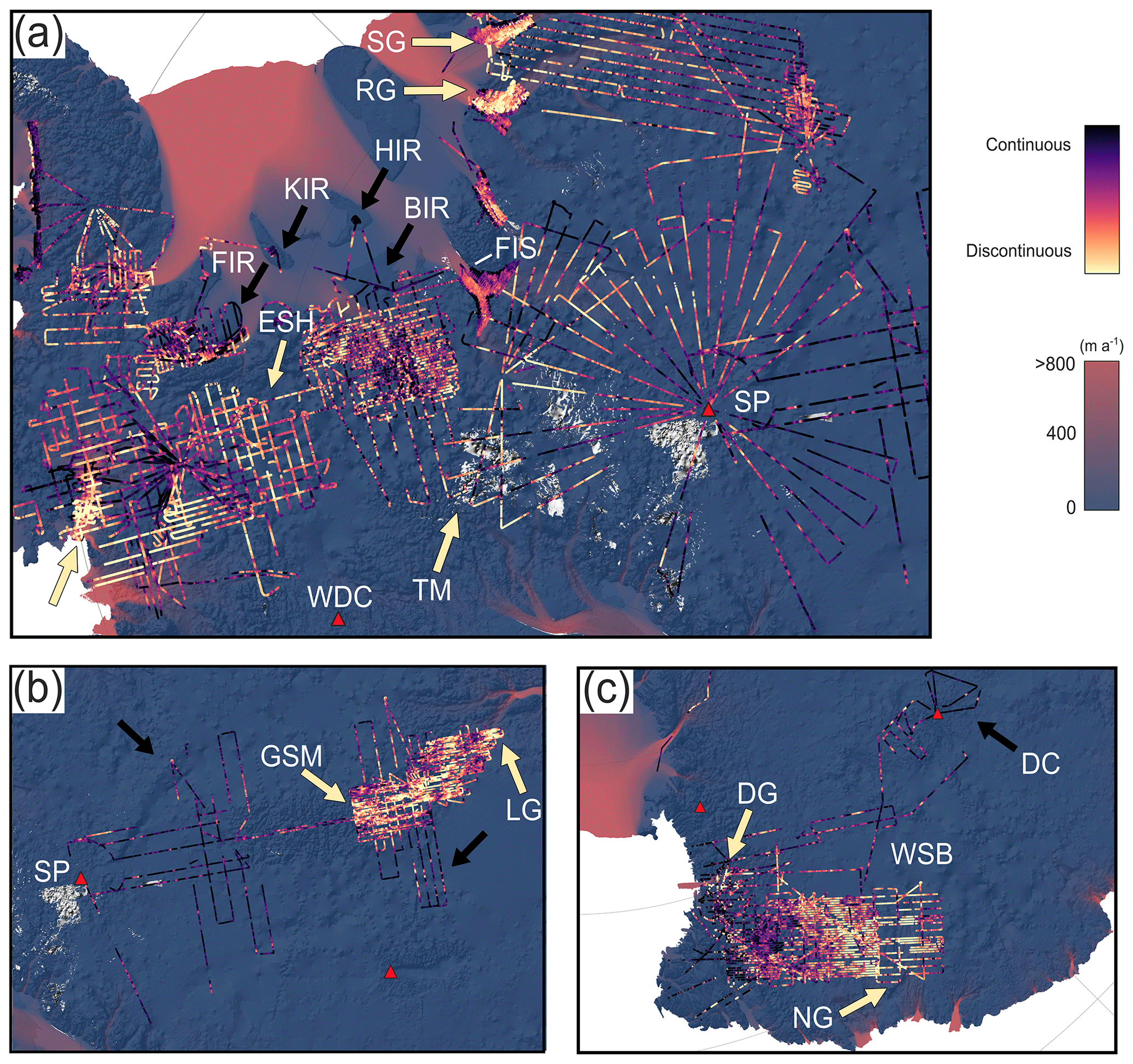
Figure 9 Zoomed-in sections of the Internal Layer Continuity Index (ICLI) shown in the black-bordered rectangles in Fig. 8. The basemap datasets and colour scales are the same as in Fig. 8. (a) ILCI results over the WAIS (including Pine Island Glacier, Rutford Ice Stream, Institute–Möller Ice Stream, and Foundation Ice Stream) and bottleneck with the EAIS (including the South Pole, Pensacola Mountains and Slessor Glacier), (b) ILCI results for the AGAP survey over East Antarctica's Dome A and South Pole, (c) ILCI results for the WISE-ISODYN survey over East Antarctica's Wilkes Subglacial Basin and Dome C. Arrows refer to locations mentioned in the text, with black arrows highlighting examples of high-layer continuity and yellow arrows low-layer continuity. As per Fig. 8, the red triangles correspond to existing deep ice cores located near the BAS radar surveys. Abbreviations correspond to locations mentioned in the text, as follows: BIR (Bungenstock Ice Rise); DC (Dome C); DG (David Glacier); ESH (Ellsworth Subglacial Highlands); FIR (Filchner Ice Rise); FIS (Foundation Ice Stream); GSM (Gamburtsev Subglacial Mountains); HIR (Henry Ice Rise); KIR (Korff Ice Rise); LG (Lambert Glacier); NG (Ninnis Glacier); RG (Recovery Glacier); SG (Slessor Glacier); SP (South Pole); TM (Transantarctic Mountains); WDC (WAIS Divide Core); WSB (Wilkes Subglacial Basin).

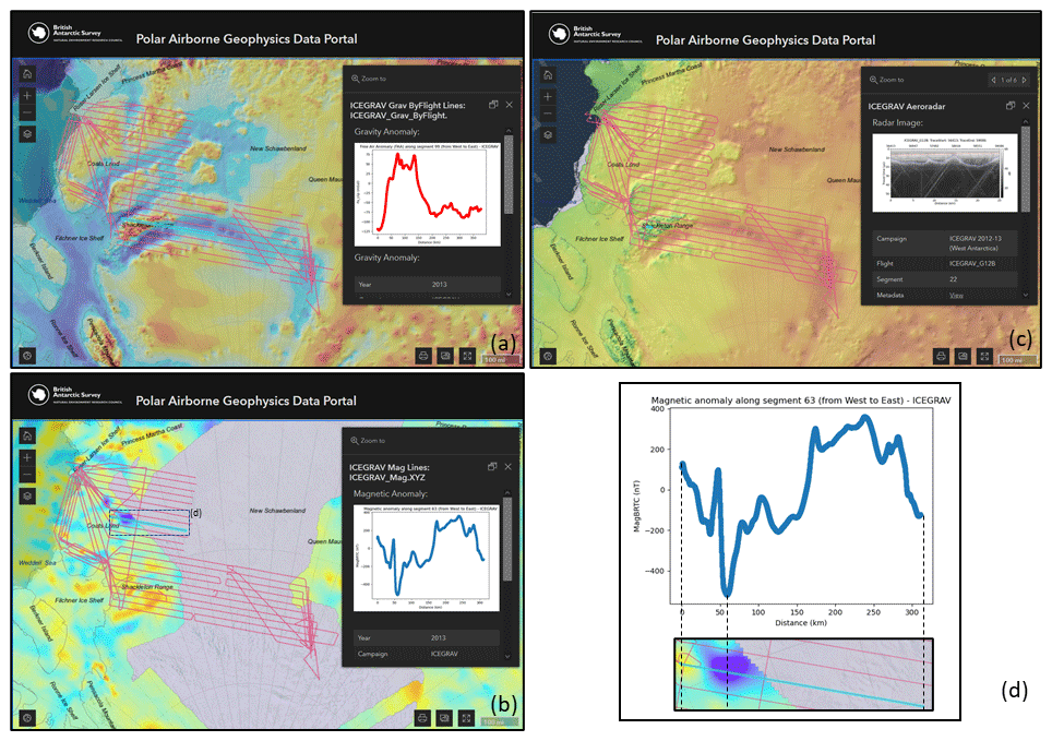
Figure 10 Screenshots of the Polar Airborne Geophysics Data Portal showing the three aerogeophysical products for the 2012–2013 ICEGRAV survey with different basemaps. (a) ICEGRAV aerogravity survey with the BEDMAP2 bed-elevation basemap. (b) ICEGRAV aeromagnetic survey with the magnetic-anomaly basemap from Goodge and Finn (2010). (c) ICEGRAV aeroradar survey with the ice-thickness basemap from BEDMAP2. (d) Magnetic anomaly along the profile highlighted in (c) with a comparison with the aeromagnetic anomaly map from Goodge and Finn (2010).

Altogether, the results presented in Figs. 8 and 9 show considerable promise for those radar datasets to be exploited further in the future, particularly with regards to tracking or otherwise characterizing the englacial architecture of the ice, as motivated by the SCAR AntArchitecture group. At present, only two BAS radar datasets (BBAS and IMAFI) have been comprehensively assessed for deep englacial layers (Karlsson et al., 2009; Ashmore et al., 2020; Ross et al., 2020; Bodart et al., 2021). Importantly, the close proximity of deep ice cores, such as the WAIS Divide (Buizert et al., 2015; Sigl et al., 2016), EPICA Dome C (EPICA Community Members, 2004), and the South Pole (Winski et al., 2019), to these newly released surveys (Fig. 8, 9) provides ready opportunities for these layers to be dated, significantly increasing their wider use for glaciological and geophysical applications (e.g. Siegert and Payne, 2004; Parrenin and Hindmarsh, 2007; Cavitte et al., 2018; Sutter et al., 2021).

5.2 Polar Airborne Geophysics Data Portal

One specificity of the platform is that it offers three types of geophysical datasets – gravity, magnetic, and radar – at the same time, geospatially. Although some surveys were acquired more than 25 years ago, they may never have been exploited or analysed fully in a form that reached peer-reviewed publications, nor combined with other geophysical data before, thereby increasing their re-usability. By publishing this resource, we anticipate that the portal and datasets will foster new research and discoveries related to our understanding of ice-sheet processes and crust and lithosphere heterogeneity beneath the Antarctic Ice Sheet.

Additionally, the portal enables users to combine the published line datasets with gridded products to compare the ability of the interpolated datasets to match the direct observations. For instance, as shown in Fig. 10 for the 2012–2013 ICEGRAV survey, the portal allows users to readily investigate the free-air gravity anomaly with the bed topography from BEDMAP2 or assess the consistency between the measured ICEGRAV magnetic anomalies and the gridded aeromagnetic product (Fig. 10). Alternatively, the quick-look radargrams can be compared with the ice-thickness and bed-elevation grid cells from BEDMAP to assess sub-kilometre variations in along- and across-flow on the radar data which may have been smoothed out in the 1 km gridded product.

With its ∼ 207 000 line-km of gravity, ∼ 338 000 line-km of magnetic, and ∼ 352 000 line-km of radar data published, the Polar Airborne Geophysics Data Portal provides a robust platform for the dissemination of the BAS aerogeophysical data. Further opportunities offered by the data portal are the potential for the platform to be used to plan future field surveys or encourage future compilation efforts based on gaps in the data coverage or quality of the data.

5.3 Future Work

Although most of data published here have already been incorporated into previous data compilations such as BEDMAP2 or ADMAP2, the more recent datasets presented here will provide useful additions to future editions of such initiatives. Examples of this are the data acquired as part of the 2012–2013 ICEGRAV aeromagnetic campaign in Dronning Maud Land where the last compilation effort of magnetic anomalies had shown a large gap (Goodge and Finn, 2010; Fig. 10), or the new ice-thickness and bed-elevation data acquired over Thwaites Glacier (2018–2020), South Pole (2015–2016), and Filchner Ice Shelf (2015–2017), which are expected to be added to the new BEDMAP3 compilation.

Even though most of the gravity, magnetic, and bed-pick data acquired since the mid-1990s are now fully published, radar data from older surveys, (1994–2004) for which the bed-pick data are published and already integrated into larger gridded products (e.g. BEDMAP; Fretwell et al., 2013), are yet to be published in full as per the more modern surveys (2004–2020) released here (see Table 3). This is primarily due to poorer data management practices at times of acquisition and less well-documented processing procedures which restrict the re-usability of these older radar datasets. Much older analogue radar data acquired on films and video tapes prior to the deployment of digital radars (i.e. pre-1994) also offer additional opportunities, although the necessity for manual digitization makes this task much more time consuming and challenging. It is worth noting, however, that many of the regions broadly covered by these older surveys have recently been re-flown using more modern instruments as part of NASA's Operation IceBridge programme (MacGregor et al., 2021), although reprocessing and modernizing older radar data can bring substantial benefits, as already demonstrated by Schroeder et al. (2019). Additional reprocessing of older radar data using modern 2-D SAR techniques would also be beneficial, as recently demonstrated on BAS data (see Castelletti et al., 2020; Chu et al., 2021).

As a result of the very flexible configuration of the PASIN-2 system, much more data can also be extracted from the raw radar files already acquired, including fully polarized data used to image ice crystal-fabric orientation for estimating ice-deformation processes (i.e. Young et al., 2021), or 3-D swath radar data used to reconstruct the sub-surface at finer resolution and without compromising on across-track resolution as for conventional 2-D data (Holschuh et al., 2020).

Combined, these will likely add further opportunities for future data releases, alongside our intention to publish newly acquired data regularly via the data portal and following the procedures detailed in this paper.

6 Data availability

All the data included in this paper are freely available via the BAS Discovery Metadata System (https://data.bas.ac.uk, British Antarctic Survey, 2022), with direct links to the datasets found in Table 3 of this paper. The user guide for the data portal and the Jupiter Notebook tutorials designed for reading the gravity, magnetic, and radar data in Python and MATLAB are freely accessible on the Jupyter Book interface (https://antarctica.github.io/PDC_GeophysicsBook, Polar Data Centre, 2022) or via the BAS GitHub repository (https://github.com/antarctica/PDC_GeophysicsBook, last access: 18 July 2022). The code used to produce the Internal Layer Continuity Index over the whole BAS radar data (Figs. 8–9) is available on the GitHub page of Julien A. Bodart (https://github.com/julbod, last access: 18 July 2022) and on Zenodo (https://doi.org/10.5281/zenodo.6858932, Bodart, 2022).

7 Conclusions

We have presented the release of 64 aerogeophysical datasets from 24 surveys flown by BAS between 1994 and 2020 over West Antarctica, East Antarctica, and the Antarctic Peninsula. Altogether, the data release consists of ∼ 450 000 line-km (or ∼ 5.3 million km²) of aerogeophysical data on gravity, magnetic, and radar measurements (including bed pick from 1994 onwards and the fully processed 2-D radar data from 2004 onwards) which have all been standardized according to the FAIR (findable, accessible, interoperable and re-usable) data principles. A new data portal, the Polar Airborne Geophysics Data Portal (https://www.bas.ac.uk/project/nagdp/, last access: 18 July 2022), and interactive, open-access tutorials written in Python and MATLAB have also been created to improve the interactivity and user accessibility of our datasets.

Aside from discussing the data acquisition and processing steps, we have demonstrated that much more information can be extracted from the newly released aerogeophysical data by assessing the continuity of englacial layering along ∼ 300 000 line-km of the ice-penetrating radar data. Using an automated layer continuity extraction method on all 10 fully published 2-D radar datasets, we have shown that large volumes of radar lines contain well-preserved englacial layering from which further glaciological and geophysical information could be extracted. We note that the analysis shown in Sect. 5.1 is only possible because the data have been comprehensively standardized and made openly accessible. Whilst we acknowledge that this type of work may suffer from a lack of funding opportunities, the results presented here would suggest that re-modernizing already-acquired data may be as important as acquiring new data. It also enables their use in emerging fields such as artificial intelligence, which rely on large amounts of standardized data.

Although all of the datasets released here have so far made a significant contribution to our understanding of past and current ice-dynamical and lithospheric influences, partly through their contributions to major international collaborative projects such as the SCAR BEDMAP and ADMAP programmes, until now they have remained largely unpublished in their full form, thus restricting the further usage of the data beyond the life cycle of the science projects. It is our hope that these newly released data will offer further research opportunities and enable the wider scientific community to benefit from the abundance of newly published aerogeophysical data over Antarctica, particularly within the context of recently established international projects such as the SCAR AntArchitecture and RINGS Action groups, the latter of which focuses primarily on fillings gaps in radar observations at the boundaries of the Antarctic Ice Sheet.

Reflecting on our collaboration between data managers and scientists, we believe that this project sets a positive example for further release of aerogeophysical data, particularly for future international initiatives that are aiming to harmonize the availability and findability of aerogeophysical data collected across Antarctica. A full list of all available datasets can be found in Table 3 of this paper, or via the BAS Discovery Metadata System (https://data.bas.ac.uk, last access: 18 July 2022).