A 41-year (1979–2019) passive-microwave-derived lake ice phenology data record of the Northern Hemisphere

Seasonal ice cover is one of the important attributes of lakes in middle- and high-latitude regions. The annual freeze-up and breakup dates as well as the duration of ice cover (i.e., lake ice phenology) are sensitive to the weather and climate; hence, they can be used as an indicator of climate variability and change. In addition to optical, active microwave, and raw passive microwave data that can provide daily observations, the Calibrated Enhanced-Resolution Brightness Temperature (CETB) dataset available from the National Snow and Ice Data Center (NSIDC) provides an alternate source of passive microwave brightness temperature (T_B) measurements for the determination of lake ice phenology on a 3.125 km grid. This study used Scanning Multichannel Microwave Radiometer (SMMR), Special Sensor Microwave/Imager (SSM/I), and Special Sensor Microwave Imager/Sounder (SSMIS) data from the CETB dataset to extract the ice phenology for 56 lakes across the Northern Hemisphere from 1979 to 2019. According to the differences in T_B between lake ice and open water, a threshold algorithm based on the moving t test method was applied to determine the lake ice status for grids located at least 6.25 km away from the lake shore, and the ice phenology dates for each lake were then extracted. When ice phenology could be extracted from more than one satellite over overlapping periods, results from the satellite offering the largest number of observations were prioritized. The lake ice phenology results showed strong agreement with an existing product derived from Advanced Microwave Scanning Radiometer for Earth Observing System (AMSR-E) and Advanced Microwave Scanning Radiometer 2 (AMSR2) data (2002 to 2015), with mean absolute errors of ice dates ranging from 2 to 4 d. Compared with near-shore in situ observations, the lake ice results, while different in terms of spatial coverage, still showed overall consistency. The produced lake ice record also displayed significant consistency when compared to a historical record of annual maximum ice cover of the Laurentian Great Lakes of North America. From 1979 to 2019, the average complete freezing duration and ice cover duration for lakes forming a complete ice cover on an annual basis were 153 and 161 d, respectively. The lake ice phenology dataset – a new climate data record (CDR) – will provide valuable information to the user community about the changing ice cover of lakes over the last 4 decades. The dataset is available at https://doi.org/10.1594/PANGAEA.937904 (Cai et al., 2021).

1 Introduction

Climate change is one of the major challenges facing humanity. New technologies and methods are urgently needed to monitor and quantify the rapid changes in climate at the regional and global scale. Lakes are closely tied to climate conditions and are characterized by many important parameters for long-term monitoring of climate change, including the coverage and duration of lake ice. For lakes located at middle and high latitudes, the spatial and temporal coverage of lake ice and key phenological events provide important information about changes in weather and climate. Lake ice phenology describes the seasonal evolution of ice cover, including the freeze-up and breakup dates, and the ice cover duration (Duguay et al., 2015; Sharma et al., 2016; Smejkalova et al., 2016). The presence or absence of lake ice affects lake–atmosphere interactions, thereby affecting hydrological and ecological processes in lakes (Duguay et al., 2006, 2015; Mishra et al., 2011; Hampton et al., 2017; Knoll et al., 2019). The coverage and duration of lake ice also affect human activities, such as transportation, fishing, and winter recreational activities (Brown and Duguay, 2010; Prowse et al., 2011; Du et al., 2017; Sharma et al., 2019). Changing climate conditions in the cold season will alter the temporal and spatial characteristics of mass (such as precipitation and suspended particles) and energy (such as solar radiation and atmospheric heat) input into the lake, thereby affecting the freeze–thaw processes of lake ice (Mishra et al., 2011). On the other hand, changes in the timing of freeze-up and breakup will cause sudden changes in lake surface properties (such as albedo and roughness) and affect the exchange between lakes and the atmosphere.

Lake ice (as well as river ice) phenology is one of the most detailed climate data records (CDRs) with the longest historical coverage. For example, the Global Lake and River Ice Phenology Database (GLRIPD) from the National Snow and Ice Data Center (NSIDC) contains ice phenology records for 865 sites, including 24 438 ice-on records and 33 370 ice-off records, where the earliest record can date back to 1443 (Benson et al., 2000). GLRIPD provides a valuable data source for the study of historical changes in river and lake ice in the Northern Hemisphere. Based on this dataset, several investigations have reported that the ice phenology of rivers and lakes in the Northern Hemisphere has been changing with trends towards later freeze-up and earlier breakup in different periods of the past century. For example, Magnuson et al. (2000) found that the freeze-up dates of river and lake ice had a delaying trend at a rate of 5.8 d per century, and the breakup dates had an advancing trend at a rate of 6.5 d per century from 1846 to 1995; moreover, the change rates of the freeze-up and breakup dates accelerated after 1950. Similarly, Benson et al. (2012) found that the freeze-up dates were occurring later at a rate of 0.03–0.16 d yr⁻¹, and the breakup dates were occurring earlier at a rate of 0.05–0.19 d yr⁻¹ from 1855 to 2005, resulting in a shortening of the ice cover duration at a rate of 0.07–0.43 d yr⁻¹. Thus far, widespread lake ice loss has been found across the Northern Hemisphere and is expected to continue in the next decades (Weyhenmeyer et al., 2011; Magnuson and Lathrop, 2014; Sharma et al., 2019; Woolway and Merchant, 2019). Also, some lakes at high latitudes have changed from permanent/multiyear ice cover to seasonal ice cover, and some lakes in warm regions have changed from seasonal ice cover to intermittent ice cover (Surdu et al., 2016; Sharma et al., 2019). However, GLRIPD sites are mainly concentrated in North America, northern Europe, and Russia. There are large areas in the world where in situ lake ice records are still lacking or incomplete (Weber et al., 2016). In addition, many sites (especially those in Canada and Russia) stopped recording freeze-up and breakup dates in the late 1980s and 1990s, resulting in a rapid decrease in the lake ice records in recent decades (Murfitt and Duguay, 2021).

Satellite remote sensing has the advantage of observing the Earth's surface over large areas at a fixed time interval and has been widely used to monitor lake ice in recent decades. Most spaceborne satellites can observe the status of lake ice based on the different signals returned by ice and water. According to the wavelength used, remote sensing of lake ice can be divided into two categories: optical remote sensing and microwave remote sensing. Optical sensors with medium resolution (ca. 250–1000 m) usually provide a short revisit period (daily) and, therefore, have been widely used to estimate lake ice phenology (Arp et al., 2013; Kropáček et al., 2013; Smejkalova et al., 2016; Weber et al., 2016). For example, the Advanced Very High Resolution Radiometer (AVHRR) reflectance data have been used to extend existing in situ observations in Canada (Latifovic and Pouliot, 2007). The Moderate Resolution Imaging Spectroradiometer (MODIS) land surface temperature product (1 km) and snow cover product (500 m) have also been used to determine lake ice status and extract lake ice phenology (Nonaka et al., 2007; Hall et al., 2010; Pour et al., 2012; Weber et al., 2016; Kropáček et al., 2013; Cai et al., 2019; Wu et al., 2021). However, optical sensors are easily affected by cloud cover and illumination conditions, which limits their ability for lake ice monitoring under cloudy weather and at high latitudes (Maslanik and Barry, 1987; Helfrich et al., 2007; Kang et al., 2012). Microwave remote sensing allows for acquisitions regardless of cloud cover and dust in the atmosphere and is not affected by illumination conditions (Engram et al., 2018; Geldsetzer et al., 2010). Active microwave provides capabilities for the monitoring of lake ice based on the difference in backscatter between lake ice and open water. For example, the European Remote Sensing Satellite (ERS)-1/2 synthetic aperture radar (SAR) (Jeffries et al., 1994; Morris et al., 1995; Duguay and Lafleur, 2003) and Radarsat-1/2 SAR (Duguay et al., 2002; Geldsetzer et al., 2010) have been successfully used to obtain lake ice status. However, existing active microwave technology is limited by the narrow swath width, relatively low temporal resolution (especially at lower latitudes), and short historical coverage, making it difficult to monitor lake ice daily at a large scale (Latifovic and Pouliot, 2007; Chaouch et al., 2014) as required by the Global Climate Observing System (GCOS; Belward et al., 2016). Passive microwave sensors can capture lake ice status based on the difference in microwave radiation emitted from lake ice and open water. Microwave radiometers mounted on existing polar-orbiting satellite platforms can provide daily observations across the Northern Hemisphere and, therefore, can be used to monitor lake ice phenology. For example, Du et al. (2017) used Advanced Microwave Scanning Radiometer for Earth Observing System and Advanced Microwave Scanning Radiometer 2 (AMSR-E and AMSR2, respectively) daily T_B data to extract lake ice phenology in the Northern Hemisphere from 2002 to 2015. The Scanning Multichannel Microwave Radiometer (SMMR), Special Sensor Microwave/Imager (SSM/I), and Special Sensor Microwave Imager/Sounder (SSMIS) data have also been used to monitor ice phenology for large lakes from 1979 to present (Ke et al., 2013; Cai et al., 2017; Su et al., 2021). However, the microwave signals naturally emitted by surface features are weak; thus, passive microwave data usually have a coarse spatial resolution (several km to tens of km), but they provide great advantages in the ice observations of oceans and large lakes (Chaouch et al., 2014; Dörnhöfer and Oppelt, 2016).

The latest Calibrated Enhanced-Resolution Brightness Temperature (CETB) dataset released by NSIDC provides passive microwave T_B data at multiple grid spacings from 25 to up to 3.125 km, including SMMR, SSM/I, SSMIS, and AMSR-E data. The enhanced-resolution images were generated using the radiometer version of the Scatterometer Image Reconstruction (rSIR) algorithm, which provides higher-spatial-resolution surface T_B images with smaller total error compared with conventional drop-in-the-bucket gridded image formation (Long and Brodzik, 2016). Due to the coarse grid spacing (25 km) of the original SMMR and SSM/I–SSMIS data, previous studies used these data to extract the ice phenology for only 22 lakes (Su et al., 2021). The newly released dataset with finer grid spacing provides an alternative data source for lake ice phenology research in the Northern Hemisphere. Moreover, in contrast to the continuous data used in previous studies (which only contained T_B data from Nimbus 7 and Defense Meteorological Satellite Program – DMSP – F08, F11, F13, and F17 satellites with a temporal overlap between satellites of less than 1 year), the CETB dataset contains data from all satellite series (Nimbus 7, F08, F10, F11, F13, F14, F15, F16, F17, F18, and F19) with greater overlap and more abundant T_B measurements.

This study uses SMMR and SSM/I–SSMIS data from the new CETB dataset to generate a lake ice phenology data record of the Northern Hemisphere from 1979 to 2019. However, two problems need to be solved: (1) how to extract lake ice phenology events from SMMR and SSM/I–SSMIS data; and (2) how to select lake ice phenology results from multiple satellites with overlapping years. The workflow behind the production of the dataset of annual ice dates and durations for 56 lakes is described. Then, the accuracy of the derived ice dates is compared against existing in situ observations and satellite-based lake ice datasets. Finally, the spatial characteristics of the lake ice phenology in the Northern Hemisphere are analyzed.

2 Data and methods

2.1 Selected lakes

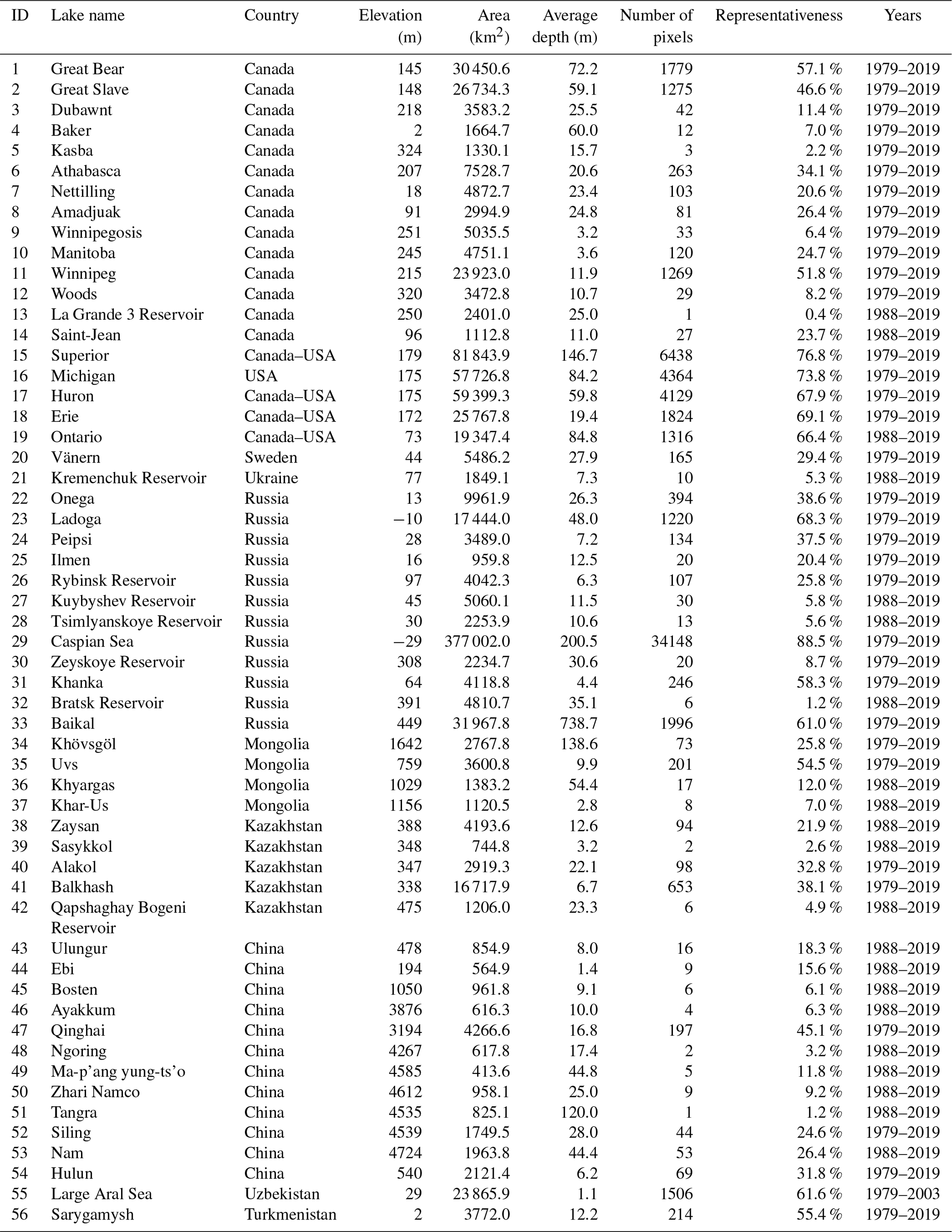
To make sure that there is at least one complete passive microwave pixel in the center of the lake, lakes with a large enough area or a nearly circular shape were selected. As a result, 56 lakes were selected as the study lakes. Lake boundaries from the European Space Agency (ESA) Lakes Climate Change Initiative (Lakes_cci) project (https://doi.org/10.5285/3c324bb4ee394d0d876fe2e1db217378, Crétaux et al., 2020) were also obtained to determine the distance of each pixel to the lake shore as to avoid land contamination (see Sect. 2.3.2 for details) (Fig. 1, Table 1). The physical characteristics of the study lakes were obtained from the HydroLAKES dataset (https://www.hydrosheds.org/page/hydrolakes, last access: 3 December 2019). Among the 56 lakes, 19 are in North America and another 37 are in Eurasia. A total of 10 lakes located in warmer regions, forming intermittent ice cover, were also contained in the study. As lakes freeze-up in autumn or winter and breakup in spring or summer, in order to simplify the description of the study period, the lake ice period is determined to be from September to August of the following year. For example, 2019 refers to the period from September 2018 to August 2019. However, the generated dataset available to users also provides calendar dates.

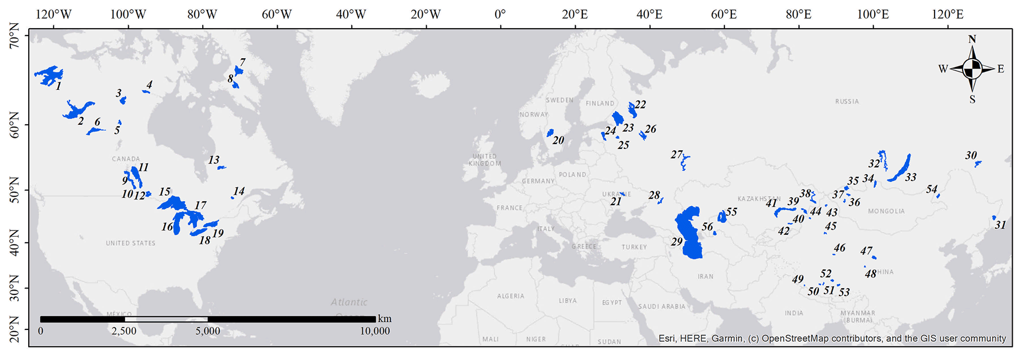
Figure 1 Location of the 56 study lakes (the names of the lakes are listed in Table 1). © OpenStreetMap contributors 2021. Distributed under the Open Data Commons Open Database License (ODbL) v1.0.

Table 1 The location and physical characteristics of the 56 study lakes as well as the number of pixels used for the lake ice phenology extraction.

2.2 Datasets

2.2.1 CETB dataset

The CETB dataset consists of gridded enhanced-resolution T_B data produced from SMMR on Nimbus 7; SSM/I on DMSP 5D-2 F8, DMSP 5D-2 F10, DMSP 5D-2 F11, DMSP 5D-2 F13, DMSP 5D-2 F14, and DMSP 5D-3/F15; SSMIS on DMSP 5D-3 F16, DMSP 5D-3 F17, DMSP 5D-3 F18, and DMSP 5D-3 F19; and AMSR-E on Aqua. For different channels, CETB provides T_B data with multiple grid spacings from 25 to 3.125 km. The enhanced-resolution images were generated using the rSIR algorithm where each pixel T_B was derived from all overlapping measurements, weighted based on the antenna measurement response function (Brodzik et al., 2020). Compared with other existing passive microwave data products, CETB provides the most complete passive microwave records with the best spatial resolution as well as other advantages, such as improvements in cross-sensor calibration and quality checks, improved projection grids, and local time-of-day processing (Brodzik et al., 2020). In this study, the 3.125 km 37 GHz H-polarized evening T_B data from all of the SMMR, SSM/I, and SSMIS satellites (except for F19 as its temporal coverage was less than 1 year) were used to extract lake ice phenology in the Northern Hemisphere (https://doi.org/10.5067/MEASURES/CRYOSPHERE/NSIDC-0630.001, Brodzik et al., 2020).

2.2.2 GLRIPD

GLRIPD contains in situ observations of ice-on and ice-off dates for 865 lakes and rivers of the Northern Hemisphere. In this database, ice on is defined as the freeze-up end date, and ice off represents the date of breakup end (Benson et al., 2000). The GLRIPD data were obtained from NSIDC (https://doi.org/10.7265/N5W66HP8, Benson et al., 2000). For comparison with lake ice phenology extracted from SMMR and SSM/I–SSMIS data, ice-on and ice-off records were extracted for the sites that have at least 10 years of overlap with study lakes (a lake may have multiple sites). As the number of sites has decreased rapidly from the 1990s, records for only 11 sites on seven lakes (Baikal, Baker, Great Slave, Onega, Superior, Winnipeg, and Ladoga) were used for comparison. It is worth noting that these are shore-based observations, so some differences in ice dates are expected against satellite-based estimates that are determined from larger sections of the lakes.

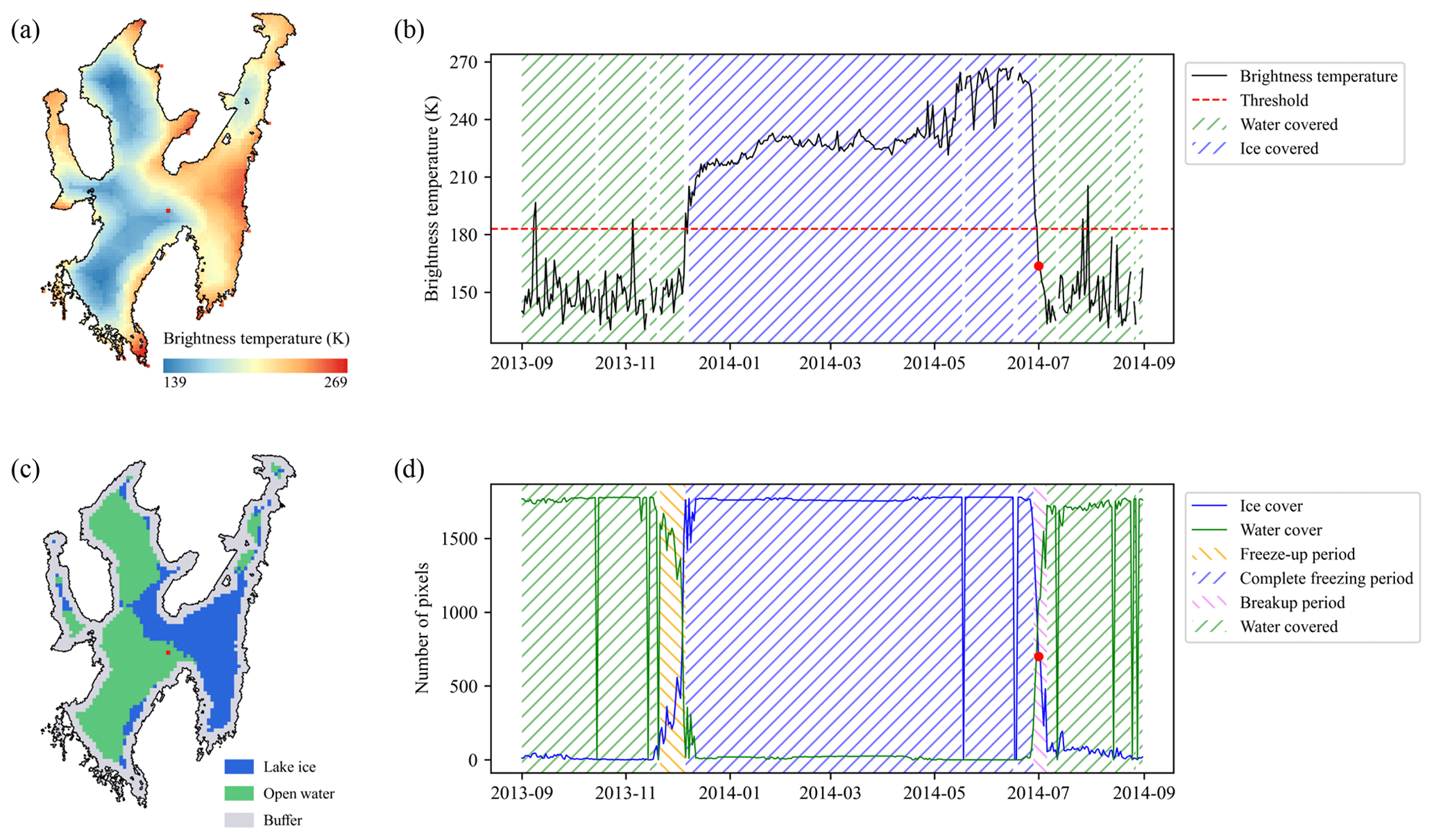
Figure 2 Example of determining the lake ice status for a pixel and extracting the ice phenology for a lake. Panel (a) shows the T_B image of Great Bear Lake on 1 July 2014. Panel (b) presents the variations in the T_B for the pixel marked in red in panel (a); the red line represents the reference T_B determined by the MTT algorithm, and the pixel was determined to be water covered on 1 July 2014 (red dot). Panel (c) is the lake ice status for all of the pixels at least 6.25 km away from the lake shore on 1 July 2014. Panel (d) shows variations in the number of lake ice and open water pixels for Great Bear Lake in 2014; the lake ice phenology was extracted using thresholds of 5 % and 95 % of the total lake pixels, and 1 July 2014 (red dot on the ice cover line) was determined to be in the breakup period.

2.2.3 AMSR-E/AMSR2 lake ice phenology product

The daily AMSR-E/AMSR2 lake ice phenology product (Du et al., 2017) was also used for comparison with the lake ice phenology results derived from the CETB dataset. The product was produced based on 36.5 GHz H-polarized T_B data, and all of the data are spatially resampled to a 5 km grid. The temporal coverage of the AMSR-E ice product is from 4 June 2002 to 3 October 2011; the temporal coverage for AMSR2 is from 24 July 2012 to 31 December 2015. The data were obtained from NSIDC (https://doi.org/10.5067/HT4NQO7ZJF7M, Du et al., 2018). For each lake, a buffer of one pixel (5 km in size) was set to remove the pixels near the lake shore that may be contaminated by land. In Du et al. (2017), the lake ice phenology dates were obtained by using the thresholds of 5 % and 95 % of the total lake pixels (see Sect. 2.3.2 for details).

2.2.4 GLERL ice cover

The Great Lakes Environmental Research Laboratory (GLERL) from the National Oceanic and Atmospheric Administration (NOAA) (https://www.glerl.noaa.gov/data/ice/#historical, last access: 23 November 2021) provides historical ice cover data for the Laurentian Great Lakes of North America from 1973 to present. The data are available from the Canadian Ice Service (from 1973 to 1988) and the United States National Ice Center (1989 to present). The annual maximum ice cover records in this database were used for comparison with those extracted from SMMR and SSM/I–SSMIS data from 1979 to 2019.

2.3 Methods

2.3.1 Determination of lake ice status for each pixel based on the Moving t test (MTT) algorithm

Moving t test (MTT) is a method for detecting abrupt changes in time series by determining whether two sub-samples are significantly different from one another (Jiang and You, 1996; Xiao and Li, 2007). To obtain the lake ice phenology from 5 km 36.5 GHz H-polarized AMSR-E/AMSR2 data, Du et al. (2017) proposed a threshold algorithm based on MTT. In this study, we used the same algorithm to extract lake ice phenology from 3.125 km 37 GHz H-polarized SMMR and SSM/I–SSMIS data from 1979 to 2019. The algorithm consists of three steps (details on the processing chain and formulas are provided in Du et al., 2017) and was applied to each passive microwave pixel:

• Step 1. For the T_B of each pixel, MTT was used to detect all of the sudden-change points in the time series.

• Step 2. Based on the results of MTT, the reference T_B values of lake ice and open water were determined, and the threshold was calculated by averaging the two reference T_B values.

• Step 3. Based on the threshold, the lake ice status of the pixel for each day was determined (Fig. 2a, b).

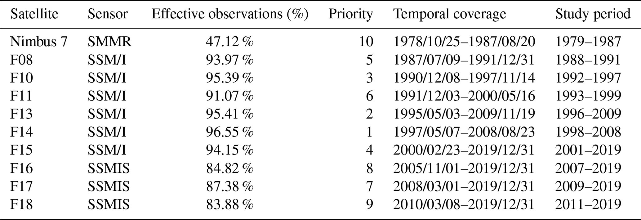
Table 2 Percentage of effective observations and the sequence for different satellites.

2.3.2 Extraction of lake ice phenology for each lake

For each pixel in a lake, the algorithm was applied for the T_B series from each satellite. Afterwards, we set a buffer of two pixels (6.25 km) from the lake shore to exclude pixels that could be contaminated by a high land fraction. The pixel size of the CETB product (3.125 km) is smaller than the footprint of the original passive microwave data (ca. 30 km), which may result in mixed water (or ice) and land in pixels near the lake shore. When the lake is water covered, the T_B for land-contaminated pixels will be higher than that of a pure water pixel, whereas the T_B will be lower than that of a pure ice pixel when the lake is ice covered. As a result, for land-contaminated pixels, the T_B difference between lake ice and water will be smaller than expected, which will eventually affect the accuracy of the MTT algorithm. Therefore, setting a buffer is necessary to exclude land-contaminated pixels. In addition, as passive microwave data have periodic sampling intervals at middle and low latitudes due to the orbital spacing, linear interpolation was used to fill the gaps in the T_B series before applying the MTT algorithm, but the interpolated data will not be used in the process of lake ice phenology extraction.

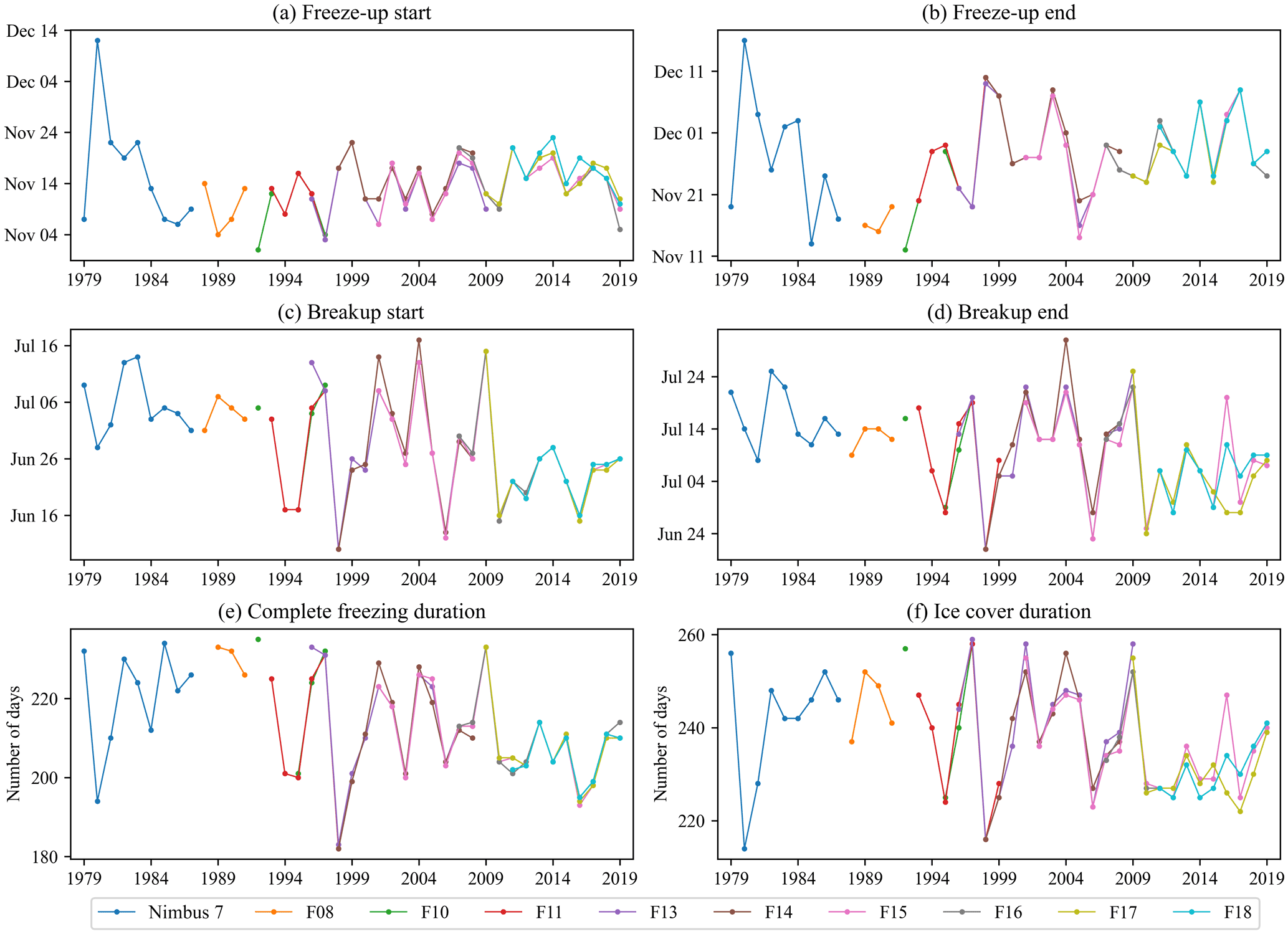
Figure 3 Lake ice phenology for Great Bear Lake extracted from multiple satellites, showing the (a) freeze-up start date, (b) freeze-up end date, (c) breakup start date, (d) breakup end date, (e) complete freezing duration, and (f) ice cover duration.

For the remaining pixels after filtering, the number of daily lake ice/lake water pixels were counted. Afterwards, thresholds of 5 % and 95 % of the total lake pixels were set to extract the lake ice phenology (Fig. 2c, d). In fall or winter, when the number of lake ice pixels is larger than 5 % of the total pixels, the lake is considered to start to form ice cover (freeze-up start), and if the number of lake ice pixels is larger than 95 %, the lake is considered to be completely frozen (freeze-up end). Similarly, in spring or summer, when the number of lake ice pixels is less than 95 %, the lake ice is considered to start to break up (breakup start), and if the number of lake ice pixels is less than 5 %, the lake is considered to be completely ice-free (breakup end). The ice duration can then be calculated: the complete freezing duration represents the period from freeze-up end to breakup start; the ice cover duration represents the period from freeze-up start to breakup end.

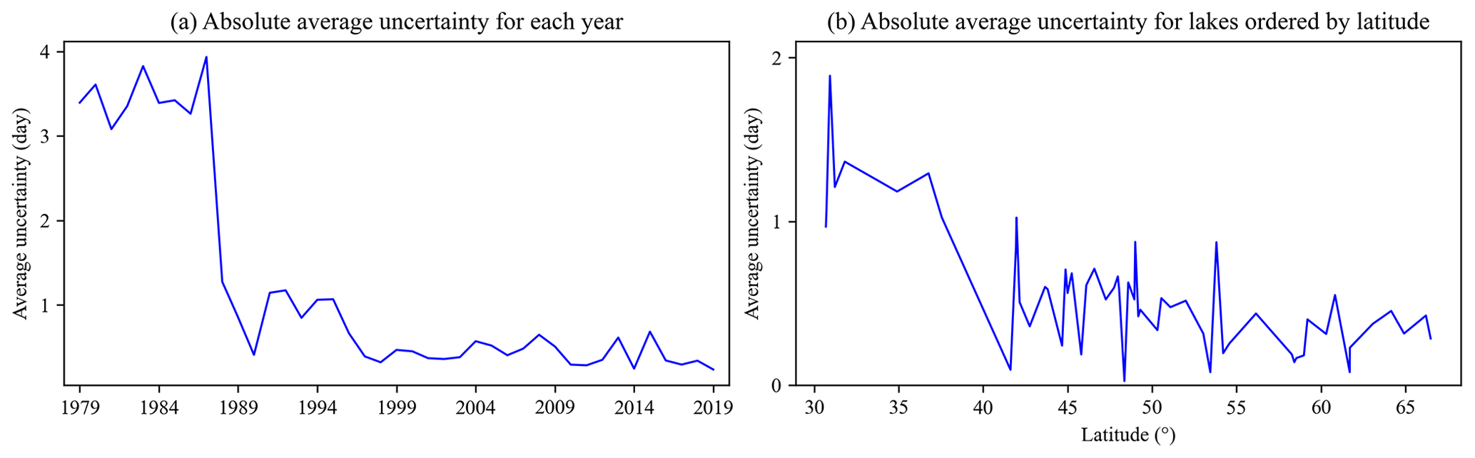
Figure 4 Differences in absolute average uncertainty among years and lakes: (a) absolute average uncertainty for each year and (b) absolute average uncertainty of lake ice phenology results extracted from SSM/I and SSMIS data for each lake ordered by latitude.

Some lakes in warmer regions did not form ice cover in certain years. For these lakes with intermittent ice cover, if no ice cover was detected throughout the year, the ice cover duration was recorded as zero; if lake ice formed but did not completely cover the lake surface, the freeze-up start and breakup end dates were extracted, while the complete freezing duration was recorded as zero. To avoid the impact of short-term weather events on the T_B, only lake ice cover persisting for more than 30 consecutive days was recorded; otherwise, it was considered that there was no ice cover detected in the year.

2.3.3 Selection of lake ice phenology results from multiple passive microwave satellites

As there are overlapping time periods for certain satellites, some years may have multiple lake ice results. Using Great Bear Lake as an example, 103-year lake ice phenology results can be obtained from all 10 satellites. However, these data were not evenly distributed within the 41 years. The lake ice phenology can be obtained simultaneously from four satellites from 2011 to 2019, while only data from one satellite can be used from 1979 to 1992 (Fig. 3).

For each satellite, only data covering a complete year (from September to August of the following year) were retained for lake ice phenology extraction, except for Nimbus 7 (with no overlapping data from other satellites) which acquired data from 25 October 1978 until 20 August 1987. Therefore, the freeze-up dates of 1987 could not be obtained for some lakes. In addition, an abnormal T_B increase in April 1986 can be observed for some lakes, which may be due to the special operations period from 2 April to 23 June 1986. To avoid possible mistakes, the breakup dates for these lakes were not extracted.

Although all of the satellites have a nominal daily temporal resolution, they have different frequencies of missing retrievals due to the polar orbit pattern and different sensor swath width. As there are no alternative data for Nimbus 7 and F08, the lake ice phenology for some lakes prior to 1992 (especially before 1987, due to the low temporal resolution and poor data quality of SMMR data) were not complete. After the launch of F11, there were at least two satellites that could retrieve T_B at the same time, which greatly improved the lake ice phenology results. As a result, lake ice phenology could be extracted over 41 years (starting in 1979 with Nimbus 7 data) for 34 lakes and over more than 30 years (starting in 1988 with F08 data) for another 21 lakes. In addition, Large Aral Sea experienced a remarkable decrease in its extent during the study period, and the increase in land pixels seriously affected the extraction of ice dates; hence, ice phenology was only extracted from 1979 to 2003 for this waterbody.

Ideally, we can obtain four ice dates (freeze-up start, freeze-up end, breakup start, and breakup end dates) in a year. However, due to data quality limitations, we failed to obtain effective observations for some lakes in some years. Using F08 as an example, we should have obtained 896 records (four ice dates for each lake in each year) for all of the 56 lakes from 1988 to 1991; however, mainly due to the continuous missing data in the winter of 1987, we finally obtained 842 ice dates. Based on the number of observations that were actually available compared with those that were expected, we calculated the percentage of effective observations (which was 93.97 % for F08; Table 2), as the basis for selecting annual ice phenology dates from overlapping results. With more missing data and a larger footprint, SMMR from the Nimbus satellite had the lowest percentage of effective observations among all of the 10 satellites. Unfortunately, there were no alternative data to improve the poor data results caused by the data quality. The six SSM/I satellites can all attain an effective observation of more than 90 %. Unexpectedly, we did not obtain the best lake ice results from the three SSMIS satellites, and their effective observation percentage values were all lower than 90 %.

We ranked the percentage of effective observations of the different satellites in a priority list with respect to obtaining lake ice phenology (Table 2). For years with multiple lake ice records extracted from more than one satellite, we prioritized the results from the satellite with the highest percentage of effective observations. Therefore, if a lake had complete lake ice results from all of the satellites, we would use the results from Nimbus 7 for 1979–1987, F08 for 1988–1991, F10 for 1992–1995, F13 for 1996–1997 and 2009, F14 for 1998–2008, and F15 for 2010–2019.

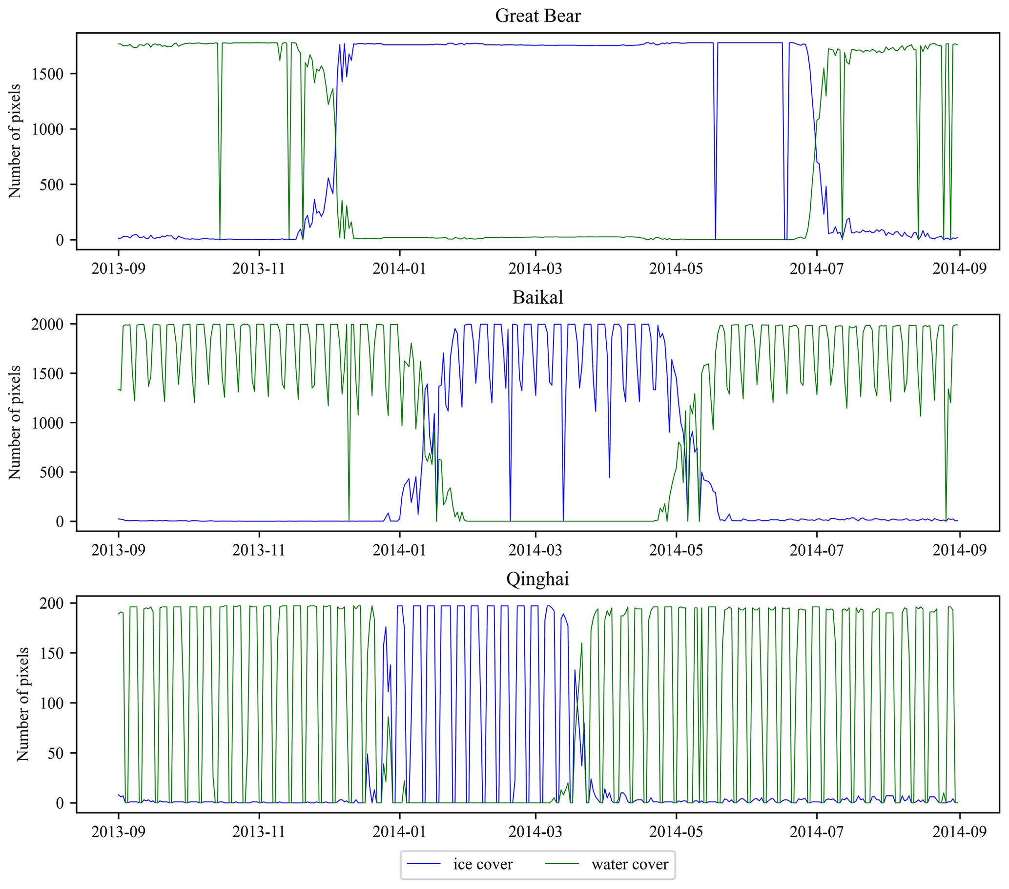
Figure 5 Variations in the number of lake ice and open water pixels for (a) Great Bear, (b) Baikal, and (c) Qinghai in 2014. The periodic fluctuations in the curves are due to the existence of orbital spacing.

Table 3 Comparisons of lake ice phenology results from different satellites. FUS, FUE, BUS, and BUE represent freeze-up start, freeze-up end, breakup start, and breakup end date, respectively.

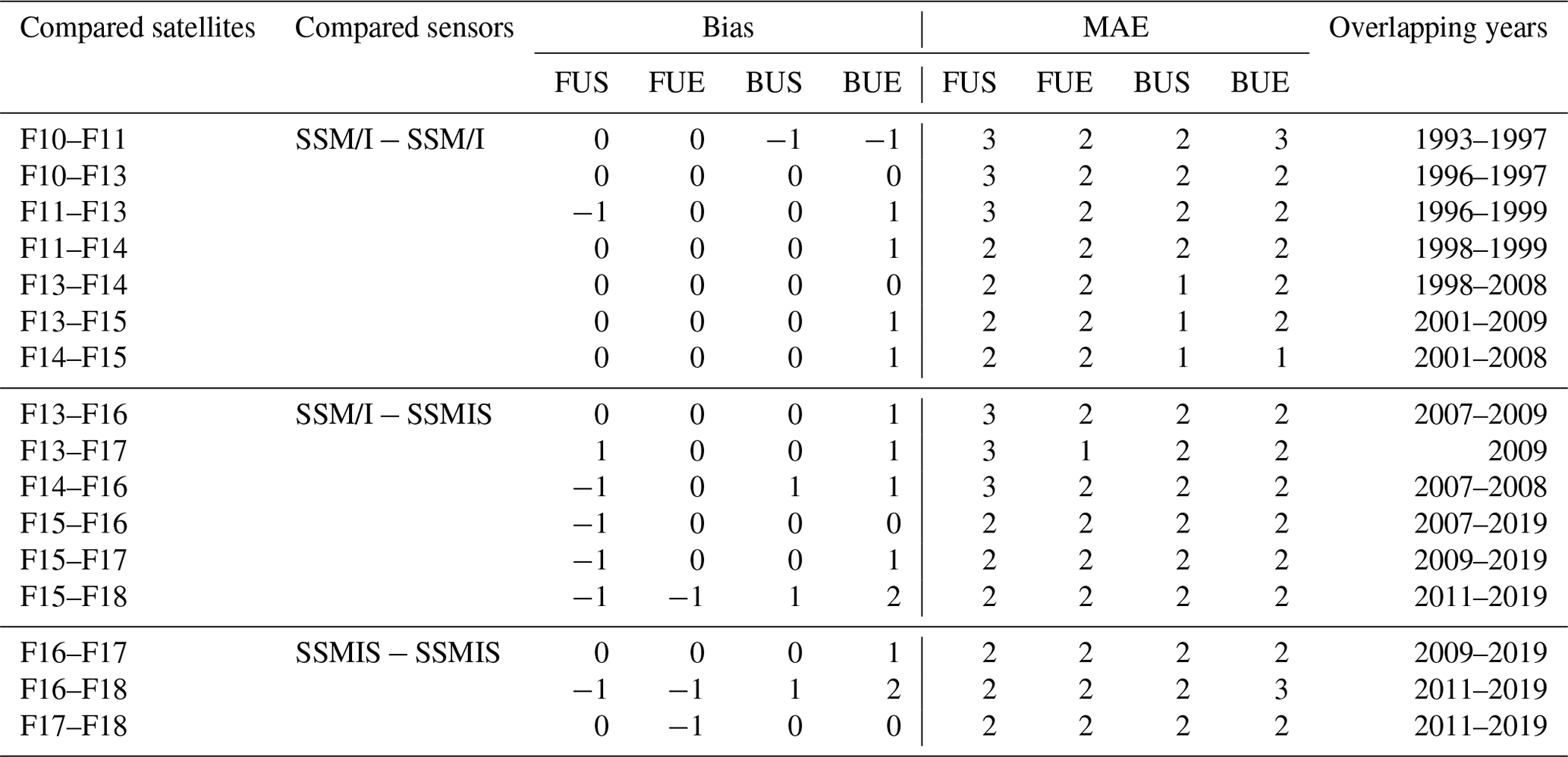
MAE: mean absolute error.

Finally, a data record of annual ice phenology for the 56 lakes from 1979 to 2019 was obtained. To increase the completeness of the lake ice phenology records, breakup dates for two lakes (Nettilling and Amadjuak) in 1987 were obtained from early F08 data (the two lakes had ice cover until late August, while Nimbus 7 data ended on 20 August 1987, and F08 started from 9 July 1987). Apart from the automatically extracted lake ice dates, 376 lake ice dates (i.e., 2.08 % of all of the records) were manually extracted to increase the ice phenology records (by setting a looser threshold in the extraction of lake ice phenology dates). Among these manually extracted lake ice dates, 263 dates were extracted from Nimbus 7 (i.e., 24.24 % of all of the Nimbus 7 records).

3 Results and discussion

3.1 Uncertainties in passive-microwave-derived lake ice phenology

There are two main error sources for lake ice phenology derived from passive microwave data: (1) the periodically missing data caused by the polar orbit operation mode of passive microwave satellites and (2) errors associated with the extraction process of lake ice phenology. Although the nominal temporal resolution of passive microwave data was 1 d, there were periodic gaps in the T_B data due to the existence of orbital spacing. Overall, the sampling frequency for SMMR data was the lowest, which may cause a maximum error of 4–6 d in the process of lake ice phenology extraction for lakes at low latitudes from 1979 to 1987. The sampling frequency greatly increased with SSM/I and SSMIS, such that the potential error caused by data gaps was 1–3 d from 1988 to 2019 (Cai et al., 2017). If missing data were encountered in the extraction process of lake ice phenology, we would obtain the next valid date as the result of lake ice phenology, so the uncertainties caused by missing data were all negative values. The average uncertainty in all records in the dataset was −1 d, and 61.70 % of the records were not affected by missing data. The lower frequency of SMMR data led to larger uncertainty (average −3 d) in the lake ice phenology results, which decreased significantly after 1988 (Fig. 4a). For each satellite, the frequencies of missing data in different regions were different: the lower the latitude, the higher the frequency of missing data. For example, there were 2 d of missing data every 4–5 d for F15, but the impact of sampling intervals on lakes at low latitudes (such as Qinghai Lake, at 36.9^∘ N) was greater than that on lakes at middle latitudes (such as Baikal Lake, at 52.2^∘ N); lakes at high latitudes, in contrast, would not be affected by the sampling intervals (such as Great Bear Lake, at 65.1^∘ N) (Fig. 5). Figure 4b shows the absolute average uncertainty for each lake ordered by latitude (records extracted from SMMR data were not included because not all lakes had records from 1979 to 1987). It can be seen that the average uncertainty is larger for lakes found at latitudes below 40^∘ N (Ayakkum, Qinghai, Ngoring, Siling, Tangra, Zhari Namco, Nam, and Ma-p'ang yung-ts'o – all on the Tibetan Plateau). In addition, the uncertainty describes the extreme error that may exist in lake ice phenology dates due to missing data, while the actual error is more likely to be smaller than the uncertainty. For example, the F08 data had 43 consecutive days of missing data from 1 December 1987 to 12 January 1988, while Lake Ladoga started to form ice cover during the period and had an ice coverage of 34 % on 13 January 1988. As a result, we recorded 13 January 1988 as the freeze-up start date of Lake Ladoga with an uncertainty of −43 d (one of the largest uncertainties), but its actual error was probably much smaller than 43 d.

Table 4 Comparison of ice-on and ice-off dates from GLRIPD records and SMMR and SSM/I–SSMIS data. Bold numbers correspond to p<0.05.

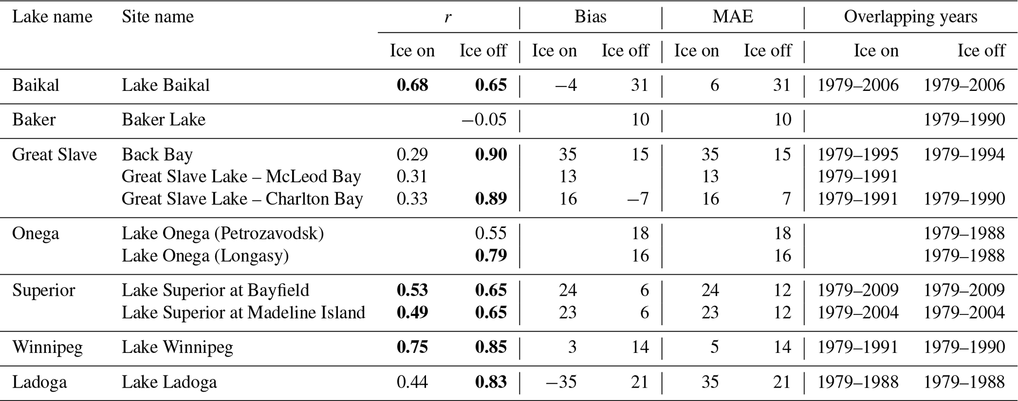
MAE: mean absolute error.

Table 5 Comparison of annual maximum ice cover of the Great Lakes from GLERL records and SMMR and SSM/I–SSMIS data. Bold numbers correspond to p<0.05.

MAE: mean absolute error.

The errors in the extraction of lake ice phenology were mainly caused by mixed pixels. Although the grid spacing for the enhanced-resolution T_B data was 3.125 km, the footprint of original data was approximately 30 km. Therefore, a single pixel may contain T_B information from a variety of different types of surface features (especially for pixels near the lake shore) (Bellerby et al., 1998; Bennartz, 1999). During the freeze-up/breakup process, a pure pixel may experience a T_B variation of up to 70–140 K (Kang et al., 2012), but the influence from land composition will result in a sharp decrease in the difference of T_B between lake ice and open water. As the MTT algorithm was mainly based on the sudden changes in the T_B series, the mixed pixels will directly affect the ice status determined by the algorithm. Before extracting the lake ice phenology dates, we set a buffer of two pixels (6.25 km) to exclude pixels near the lake shore. This is a compromise between removing more mixed pixels and extracting ice phenology for more lakes. However, the setting of a buffer will cause the loss of T_B information near the lake shore. Based on the number of pixels we used and the lake area, we calculated the representativeness of the pixels for each lake (Table 1). Depending on the lake area and shore complexity as well as the possible existence of islands on the lake, the representativeness of the pixels ranged from 0.4 % (La Grande 3 Reservoir) to 88.5 % (Caspian Sea). For lakes with a low representativeness, the setting of the buffer may result in a non-negligible error in the lake ice phenology results which is hard to quantify. As the freeze-up and breakup of ice cover usually starts from the lake shore (especially for the freeze-up), the beginning signals of freeze-up and breakup extracted from the retained pixels may later be compared with the actual ice conditions, whereas the ending signals may be earlier.

In addition, for each pixel, we only determined whether the pixel was covered by lake ice or not. However, the area for a single passive microwave pixel is 9.77 km², and the water (or ice) within this area may not freeze-up (or breakup) at the same time. Before the T_B exceeds (or falls below) the threshold, the lake surface within the pixel may have already started to freeze-up (or breakup), and this process may not end even after we detect the ice-covered (or water-covered) signal. When the lake area is large enough, the gradual freeze-up or breakup within the pixel can be ignored; however, for lakes with few available pixels and low representativeness, it may lead to certain deviations in the lake ice phenology results, similar to the effect of setting a buffer.

Furthermore, during application of the MTT algorithm, multiple smoothing approaches were applied to the original T_B series to exclude potentially dynamic T_B changes caused by short-term weather events. For example, when using MTT to judge whether there was a sudden T_B change on a certain day, the T_B of 20 d before and after that day were averaged to make the comparison (Du et al., 2017). As a result, the MTT algorithm may be insensitive to short-term ice cover or frequent melt–refreeze events during the breakup or freeze-up seasons. The 37 GHz H-polarized data are sensitive to wind-induced surface roughness during the open water period (Kang et al., 2012); this effect can also be attenuated by smoothing approaches, but may still lead to errors in lake ice phenology results. In addition, we only kept the lake ice phenology results with ice cover persisting for more than 30 consecutive days, which may also lead to some lakes with short-term ice cover being recorded as ice-free waterbodies. Du et al. (2017) also pointed out that relatively small T_B increases caused by thin ice may not be detectable using the MTT algorithm. Overall, the data and algorithm limitations may lead to an underestimation of the ice cover duration, especially for small lakes with irregular shapes and short-term ice cover.

Therefore, we adopted an automatic algorithm to extract lake ice phenology dates from all of the platforms for all of the lakes and then prioritized the lake ice phenology results extracted from the satellite with a higher percentage of effective observations, which was in order to ensure the comparability of lake ice phenology results among lakes and the consistency of the time series. Despite the uncertainties and inevitable errors caused by the periodically missing data and mixed pixels, the lake ice phenology derived from SMMR and SSM/I–SSMIS can provide reliable information about the differences among lakes and the variations in time series.

3.2 Comparisons of lake ice phenology results from multiple satellites

For all of the satellite pairs with overlapping years, we calculated the bias and mean absolute error (MAE) of the overlapping results. Different satellites can obtain lake ice dates with a bias of −1 to 2 d and an MAE of 1 to 3 d. The freeze-up end and breakup start dates extracted from different satellites had relatively higher consistencies than freeze-up start and breakup end dates (Table 3). The same conclusion can be drawn from the example of Great Bear Lake (Fig. 3). The differences among the satellites were the reason that we decided to use a priority list to determine the lake ice phenology from overlapping results instead of calculating their average values or choosing the earliest freeze-up dates and latest breakup dates. The lake ice phenology determined by the satellite priority can be more consistent and comparable among different years and different lakes, which is more beneficial for analyzing their spatial differences and change trends.

Figure 6 Box plot of the (a) r, (b) bias, and (c) mean absolute error (MAE) results of the comparison between the lake ice phenology dates extracted from the AMSR-E/AMSR2 product and SMMR and SSM/I–SSMIS data.

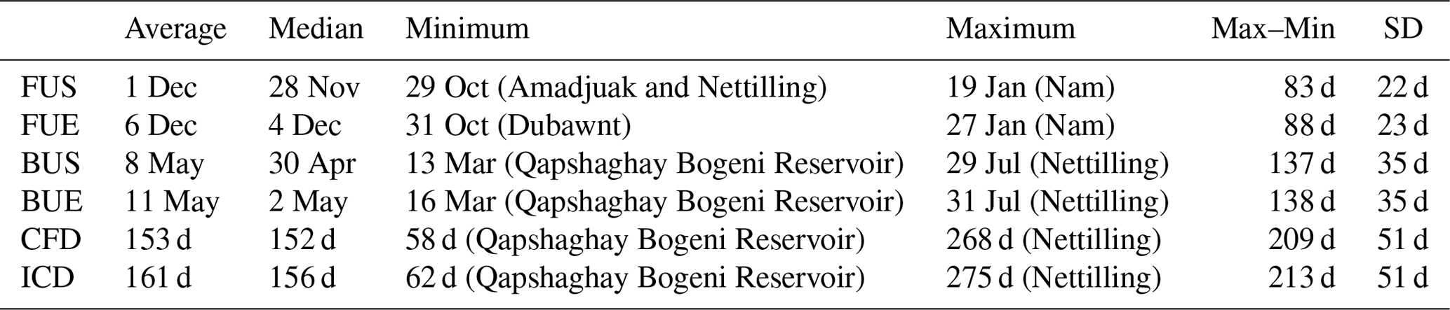
Table 6 Average, median, minimum, maximum, extreme difference (Max–Min), and standard deviation (SD) values of lake ice phenology in the Northern Hemisphere. FUS, FUE, BUS, BUE, CFD, and ICD represent the freeze-up start date, freeze-up end date, breakup start date, breakup end date, complete freezing duration, and ice cover duration, respectively.

3.3 Comparisons with existing lake ice datasets

3.3.1 Comparisons with in situ observations

The lake ice dates recorded in the GLRIPD were compared with the results extracted from SMMR and SSM/I–SSMIS data. As the ice-on and ice-off dates in the GLRIPD represent the first date of complete ice cover and the last date of the breakup process, respectively, we used the freeze-up end and breakup end results to make the comparison. For Lake Superior and Ladoga, which had incomplete freeze-up end records, freeze-up start dates were used instead. Only the lake ice records with an overlapping time of more than 10 years were selected for the comparison. As a result, ice-on dates for five lakes (8 sites) and ice-off dates for seven lakes (10 sites) were compared, and the correlation coefficient (r), mean difference (bias), and mean absolute error (MAE) were calculated (Table 4). It can be seen that the ice-on dates for 4 out of 8 sites and the ice-off dates for 8 out of 10 sites from GLRIPD are significantly consistent with the lake ice dates from SMMR and SSM/I–SSMIS data (Table 4). The main reason for the difference between lake ice dates from in situ observations and passive microwave is tentatively attributed to their different observation ranges. In situ records rely on observations of the lake ice status visible from lake shores by human observers, whereas passive microwave satellites record T_B from the entire lake surface (here, within the predefined buffer); however, a follow-up investigation is indeed needed to quantify differences between in situ observations with satellite-derived time series. As breakup usually occurs more rapidly than freeze-up (Livingstone, 1997), the ice-off dates from the two datasets were more consistent than the ice-on dates (Table 4). With the decrease in in situ observation sites globally since the 1980s, there has been a shift towards the increased use of remote sensing technology for lake ice monitoring (Murfitt and Duguay, 2021). Satellite observations can complement, if not supersede, in situ observations to investigate interannual variations and trends in lake ice phenology in recent decades.

3.3.2 Comparisons with the AMSR-E/AMSR2 lake ice phenology product

The AMSR-E/AMSR2 lake ice phenology product (Du et al., 2017) was also used to extract the ice dates for the study lakes from 2003 to 2015 (except for 2012 due to the data gap between AMSR-E and AMSR2 from 4 October 2011 to 23 July 2012), and the r, bias, and MAE values compared with the ice dates from SMMR and SSM/I–SSMIS data were calculated for each lake (Fig. 6). The freeze-up start and breakup end dates for 55 lakes (except for Large Aral Sea, which has no records after 2003) and the freeze-up end and breakup start dates from 49 lakes (except for Large Aral Sea and some lakes without complete ice cover in winter) were compared. The breakup dates had an overall higher consistency between the results from the two datasets than the freeze-up dates (Fig. 6a). Among them, the freeze-up start dates for 49 lakes, the freeze-up end dates for 45 lakes, the breakup start dates for 46 lakes, and the breakup end dates for 53 lakes were significantly consistent. The biases for all pairs of freeze-up start, freeze-up end, breakup start, and breakup end dates were 2, −2, 3, and 0 d, respectively (Fig. 6b). The freeze-up start and breakup start dates obtained from SMMR and SSM/I–SSMIS data were approximately 2–3 d later than the results from AMSR-E/AMSR2 data, whereas the freeze-up end and breakup end dates were slightly earlier than those from AMSR-E/AMSR2 data. Although SMMR, SSM/I, and SSMIS from the CETB dataset have a grid spacing of 3.125 km, their original resolution was ca. 30 km, whereas AMSR-E/AMSR2 data (5 km grid spacing) have a finer original spatial resolution of about 10 km (14 km ×8 km for AMSR-E and 12 km ×7 km for AMSR2). The buffers used to extract lake ice phenology dates were also different: the buffer set for SMMR and SSM/I–SSMIS data was 6.25 km, whereas that set for AMSR-E/AMSR2 data was 5 km. Therefore, AMSR-E/AMSR2 data captured more information near the lake shore than SMMR and SSM/I–SSMIS data (the representativeness of AMSR-E/AMSR2 data ranged from 1.9 % to 89.8 %, with an average of 5.0 % higher than that of SMMR and SSM/I–SSMIS data), which led to the directional differences between the lake ice phenology dates extracted from the two datasets. The MAE values for all of the pairs of freeze-up start, freeze-up end, breakup start, and breakup end dates were 4, 3, 3, and 2 d, respectively (Fig. 6c). Among the four lake ice dates, the MAE of the freeze-up start dates was the largest, whereas that of the breakup end dates was the smallest. This is also due to the fact that the lake can take a longer time to freeze-up in early winter, but after the lake starts to breakup in spring, the lake surface will be completely ice-free in a short time (Livingstone, 1997). Overall, despite the different spatial resolution and sensor characteristics, the lake ice phenology results obtained from the two passive microwave data products are highly consistent.

3.3.3 Comparisons with the GLERL ice cover records

Apart from lake ice phenology dates, the annual maximum ice cover was extracted for seven intermittently ice-covered lakes with more than 1000 pixels (Superior, Huron, Michigan, Erie, Ontario, Caspian Sea, and Ladoga) from SMMR and SSM/I–SSMIS data and compared to that from the five Great Lakes contained in the GLERL historical ice cover records. Ice cover maximums from SMMR and SSM/I–SSMIS data and GLERL were significantly consistent for these lakes (Table 5). Among them, the ice cover values extracted for Erie showed the lowest bias and MAE, due to the fact that this lake experiences an extensive ice coverage in winter (Fig. 7d). The remaining four lakes all showed a negative bias, indicating that the ice cover values extracted from SMMR and SSM/I–SSMIS data were usually smaller than the actual situation. This is not only because a buffer of 6.25 km was used to exclude pixels near the lake shore, which happens to be the place where lake ice forms first, but short-term ice cover, which was common on these lakes, was also difficult to detect with the MTT algorithm. This is also why the lake was sometimes 100 % ice covered but only partial coverage was detected by SMMR and SSM/I–SSMIS data. Using 2014 as an example, we recalculated the daily ice cover from the GLERL ice charts over the same areas as the SMMR and SSM/I–SSMIS data to make a comparison of daily ice cover changes from the two datasets (Fig. 8). High consistency in the daily ice cover percentage can be seen for Erie, Huron, and Superior; however, for Michigan and Ontario, a similar change pattern but lower ice cover was obtained from SMMR and SSM/I–SSMIS data compared with the GLERL records because the short-term ice cover on Michigan and Ontario in February and March was not detected by the MTT algorithm after the smoothing approaches were applied (Fig. 8). Although it is difficult to capture the short-term changes in ice cover, the algorithm showed good performance with respect to obtaining ice cover for lakes with long-term ice cover.

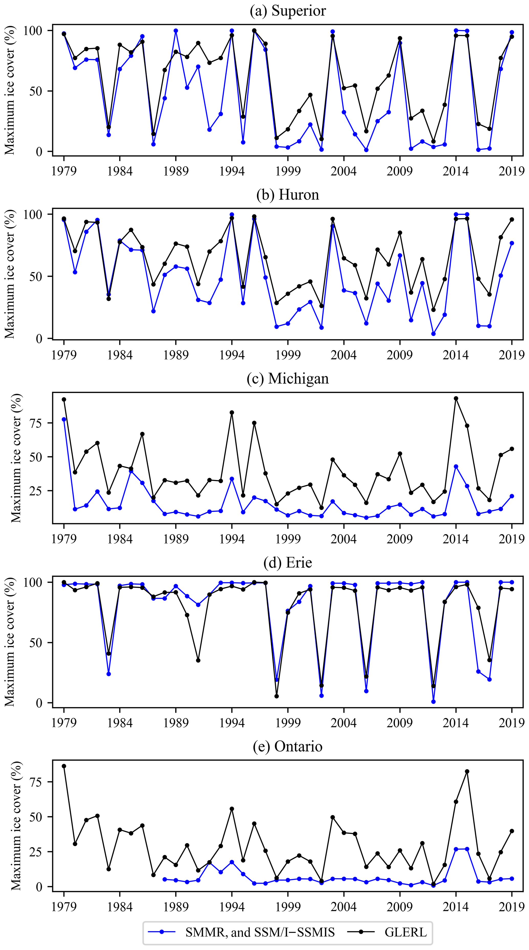
Figure 7 Comparisons of the annual maximum ice cover (percentage of lake area) of the Great Lakes from the GLERL records and SMMR and SSM/I–SSMIS data: (a) Superior, (b) Huron, (c) Michigan, (d) Erie, and (e) Ontario.

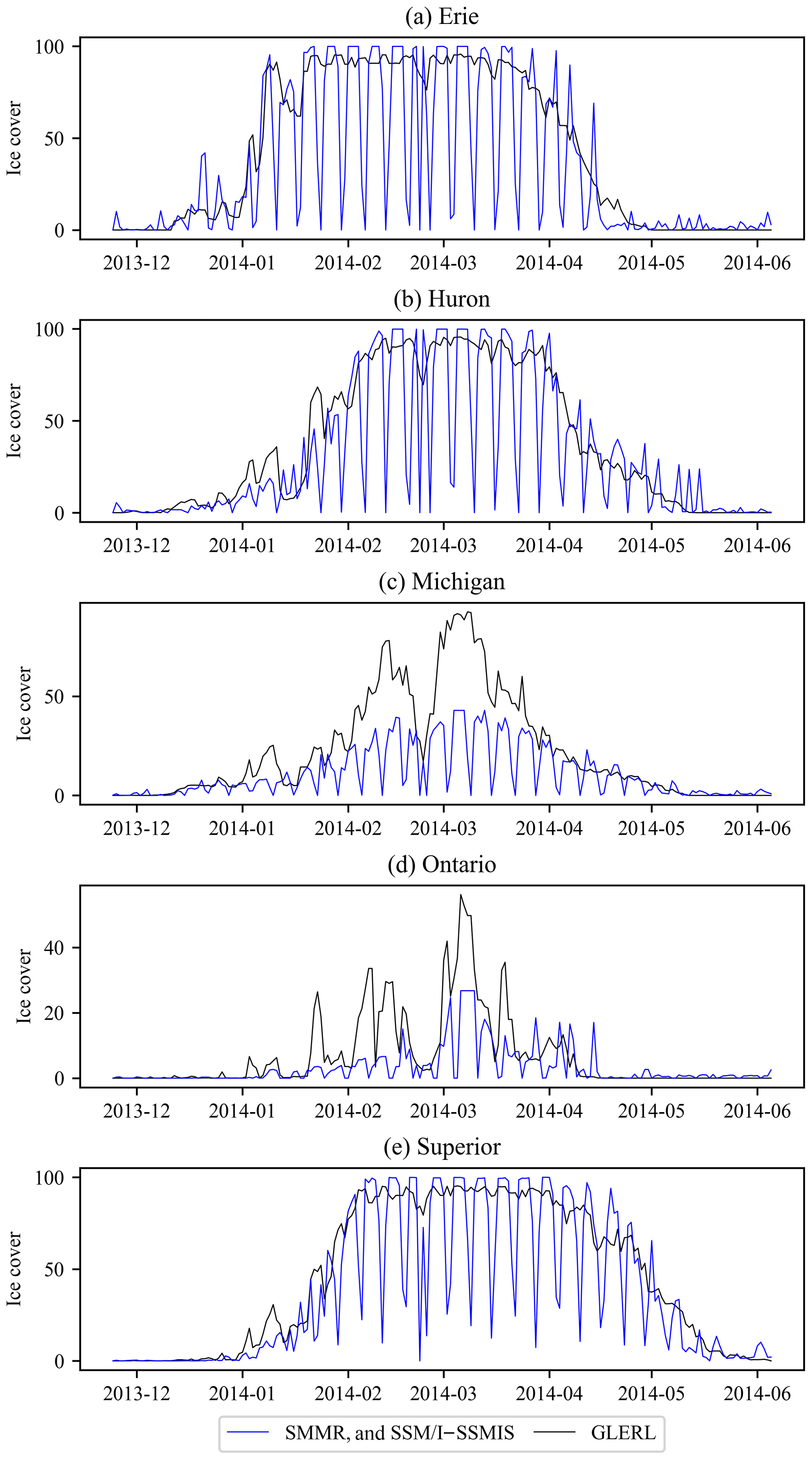
Figure 8 Comparisons of the daily ice cover (percentage of lake area) of the Great Lakes from the GLERL records and SMMR and SSM/I–SSMIS data in 2014: (a) Superior, (b) Huron, (c) Michigan, (d) Erie, and (e) Ontario.

3.4 Lake ice phenology in the Northern Hemisphere

Among the 56 study lakes, 45 lakes experienced annual ice cover during their entire lake ice phenology records, and the remaining 11 lakes had no ice detected for 1 year or more. Note that, as we only selected the pixels 6.25 km away from the lake shore to extract the lake ice phenology, it is possible that some lakes had ice cover near the lake shore, but we did not obtain the information. The average date and days of the respective ice dates and durations for each lake during their entire lake ice phenology records were calculated (relative to 1 September) and are shown in Fig. 9. In order to avoid bias in the statistics for the lakes with no ice detected in some years, only the 45 lakes with annual ice cover were included. A total of 2 of the 45 lakes (Caspian Sea and Ladoga) did not have annual complete ice cover in winter; hence, only their freeze-up start dates, breakup end dates, and ice cover durations were calculated (Fig. 9). In addition, the statistical results of ice phenology for the 45 lakes are shown in Table 6, including their average, medium, minimum (earliest/shortest), and maximum (latest/longest) date/days as well as the extreme difference (maximum–minimum) and standard deviation. Here, we can see that the period of ice formation is from the end of October to January of the next year, and the period of ice breakup is from mid-March to late July. Overall, the differences among freeze-up dates are smaller than those for breakup dates (with smaller extreme differences and standard deviations; Table 6), but the spatial characteristics of breakup dates are more consistent with latitude (Fig. 9). Different lakes experienced a complete freezing duration ranging from 58 to 268 d (average 153 d) and an ice cover duration ranging from 62 to 275 d (average 161 d). Lakes in low-latitude Eurasia had the shortest ice cover durations, whereas lakes in northern Canada had the longest ice cover durations (Fig. 9).

Figure 9 Average date/days of ice phenology for the study lakes for their entire lake ice phenology records extracted from SMMR and SSM/I–SSMIS data: (a) freeze-up start date, (b) freeze-up end date, (c) breakup start date, (d) breakup end dates, (e) complete freezing duration, and (f) ice cover duration. © OpenStreetMap contributors 2022. Distributed under the Open Data Commons Open Database License (ODbL) v1.0.

4 Data availability

The annual lake ice phenology records for the 56 study lakes are available at https://doi.org/10.1594/PANGAEA.937904 (Cai et al., 2021). Calendar dates of freeze-up start, freeze-up end, breakup start, and breakup end as well as the days of complete freezing duration and ice cover duration are provided in the dataset. Additional data of annual maximum ice cover for the Great Lakes, Caspian Sea, and Ladoga are also provided. As the original data (the CETB dataset) was updated to the end of 2019, we currently provide the lake ice phenology from 1979 to 2019. The CETB dataset was obtained from https://doi.org/10.5067/MEASURES/CRYOSPHERE/NSIDC-0630.001 (Brodzik et al., 2020). The GLRIPD data were obtained from https://doi.org/10.7265/N5W66HP8 (Benson et al., 2000). The AMSR-E/AMSR2 lake ice phenology product was obtained from https://doi.org/10.5067/HT4NQO7ZJF7M (Du et al., 2018). The GLERL ice cover data were obtained from the National Oceanic and Atmospheric Administration (https://www.glerl.noaa.gov/data/ice/#historical, (last access: 23 November 2021, NOAA Great Lakes Environmental Research Laboratory, 2021). The lake boundaries were obtained from the European Space Agency (ESA) Lakes Climate Change Initiative project (https://doi.org/10.5285/3c324bb4ee394d0d876fe2e1db217378, Crétaux et al., 2020). The physical characteristics of the study lakes were obtained from the HydroLAKES dataset (https://www.hydrosheds.org/page/hydrolakes last access: 3 December 2019, Messager et al., 2016).

5 Conclusions

This study used passive microwave SMMR and SSM/I–SSMIS data available on a 3.125 km grid from the CETB dataset to extract the ice phenology for 56 lakes in the Northern Hemisphere from 1979 to 2019. An automatic threshold algorithm based on the MTT method was applied to determine the lake ice status for each pixel, and a buffer of 6.25 km was set to exclude pixels with high land contamination. Then, ice phenology dates were extracted for each lake using the thresholds of 5 % and 95 % of the total pixels. To keep the lake ice phenology consistent and comparable among different years and different lakes, for the overlapping lake ice phenology results extracted from multiple satellites, we prioritized the results from the satellite with the highest percentage of effective observations.

The main error sources of the lake ice phenology extracted from SMMR and SSM/I–SSMIS data were attributed to the periodically missing data at middle and low latitudes caused by the polar orbit operation mode and the mixed pixels caused by the original coarse spatial resolution of the satellite acquisitions. Ice phenology results for the lakes at low latitudes and/or with small areas tend to be characterized by a larger uncertainty. The switch between sensors and satellites over the time series also resulted in certain differences in the lake ice phenology results, with a bias ranging from −1.30 to 2.00 d and an MAE from 1.20 to 3.13 d.

The lake ice phenology results extracted from SMMR and SSM/I–SSMIS data were compared to the ice dates from in situ observations and an AMSR-E/AMSR2-derived lake ice phenology product. Compared to in situ observations, the ice-on dates for 4 out of 8 sites, and the ice-off dates for 8 out of 10 sites were significantly consistent. The differences between the in situ observations and the lake ice phenology extracted in this study were mainly due to the different fields of view of human observers versus satellite instruments. As for the AMSR-E/AMSR2 product, the ice dates showed strong agreement, with biases ranging from −1.98 to 2.98 d and MAE values ranging from 2.21 to 3.60 d. The different spatial resolution and sensor characteristics of the AMSR-E/AMSR2 and the SMMR and SSM/I–SSMIS data can explain the biases between the ice dates. Annual maximum ice cover determined for the Great Lakes also showed significant consistencies compared to the GLERL historical ice cover records.

From 1979 to 2019, the average complete freezing duration and ice cover duration for all lakes forming an annual ice cover were 153 d (58–268 d for individual lake) and 161 d (62–275 d). Lakes in the low latitudes of Central Asia had the shortest ice durations, whereas lakes in northern Canada had the longest ice durations.

The new dataset consists of lake ice phenology records derived from SMMR and SSM/I–SSMIS data from 1979 to 2019. Lake ice phenology (freeze-up, breakup, and ice cover duration) is a robust indicator of climate change. The analysis-ready dataset is available to the science/user community to investigate, among several possible topics, the following: (1) trends and interannual variability in lake ice phenology across the Northern Hemisphere in response to climate change and atmospheric teleconnections patterns; and (2) the impact of changing ice phenology on local/regional weather, climate and hydrology, aquatic ecosystems, and cultural and socioeconomic activities.

Finally, regular updates of the lake ice phenology data record are planned with future releases of the CETB dataset. Work is also underway on further improving the lake ice phenology retrieval algorithm and product as well as on the possibly of adding more lakes in a future release.