Third revision of the global surface seawater dimethyl sulfide climatology (DMS-Rev3)

This paper presents an updated estimation of the bottom-up global surface seawater dimethyl sulfide (DMS) climatology. This update, called DMS-Rev3, is the third of its kind and includes five significant changes from the last climatology, L11 (Lana et al., 2011), that was released about a decade ago. The first change is the inclusion of new observations that have become available over the last decade, creating a database of 873 539 observations leading to an ∼ 18-fold increase in raw data as compared to the last estimation. The second is significant improvements in data handling, processing, and filtering, to avoid biases due to different observation frequencies which result from different measurement techniques. Thirdly, we incorporate the dynamic seasonal changes observed in the geographic boundaries of the ocean biogeochemical provinces. The fourth change involves the refinement of the interpolation algorithm used to fill in the missing data. Lastly, an upgraded smoothing algorithm based on observed DMS variability length scales (VLS) helps to reproduce a more realistic distribution of the DMS concentration data. The results show that DMS-Rev3 estimates the global annual mean DMS concentration to be ∼ 2.26 nM (2.39 nM without a sea-ice mask), i.e., about 4 % lower than the previous bottom-up L11 climatology. However, significant regional differences of more than 100 % as compared to L11 are observed. The global sea-to-air flux of DMS is estimated at ∼ 27.1 TgS yr⁻¹, which is about 4 % lower than L11, although, like the DMS distribution, large regional differences were observed. The largest changes are observed in high concentration regions such as the polar oceans, although oceanic regions that were under-sampled in the past also show large differences between revisions of the climatology. Finally, DMS-Rev3 reduces the previously observed patchiness in high productivity regions. The new climatology, along with the algorithm, can be found in the online repository: https://doi.org/10.17632/hyn62spny2.1 (Mahajan, 2021).

1 Introduction

Dimethyl sulfide (DMS) is a volatile compound found in the global oceans, and its biogeochemical cycle plays an important role in the Earth's climate system (Andreae and Crutzen, 1997; Charlson et al., 1987). It is primarily a by-product of phytoplankton growth and marine microbial food web interactions (Simó, 2001). DMS is produced by the breakdown of the phytoplankton intracellular metabolite dimethylsulfoniopropionate (DMSP), either in the algal cell or through microbial catabolism of the DMSP released due to physiological stress or mortality (Kiene et al., 2000; Stefels et al., 2007). This produced DMS is either oxidized by photochemical reactions or metabolized by bacteria (Toole et al., 2003), leaving a small portion that is released into the atmosphere as gaseous DMS (Galí and Simó, 2015; Simó, 2001). The DMS emitted from the surface ocean is responsible for up to 70 % of the natural sulfur emissions into the global atmosphere (Andreae and Raemdonck, 1983; Carpenter et al., 2012). Oxidation of DMS takes place in the atmosphere and yields sulfuric and methanesulfonic acids, which eventually lead to the formation of sulfate aerosols that can grow to act as cloud condensation nuclei (CCN) (Andreae and Barnard, 1984; Pazmiño et al., 2005). New CCN can make clouds brighter, thus establishing a feedback loop between phytoplankton and cloud albedo popularly known as the CLAW hypothesis (Charlson et al., 1987). While some studies based on large-scale observations of ocean surface DMS provided partial support for the CLAW hypothesis (Vallina and Simó, 2007), other studies based on model sensitivity analysis of the hypothesis have challenged it (Quinn and Bates, 2011; Woodhouse et al., 2010, 2013). However, even if the feedback loop is not as strong as previously envisaged, DMS emissions contribute towards a large fraction of aerosols in the remote oceanic environment (Quinn et al., 2017) and its emissions need to be quantified accurately to improve our understanding of climate sensitivity, the current climate (Carslaw et al., 2013) and to improve the accuracy of future projections (Wang et al., 2021).

Acknowledging the significance of oceanic DMS, the scientific community has striven to reproduce an accurate representation of the global atmospheric and seawater DMS concentrations, and more importantly, the ocean–atmosphere flux on a global scale. To compute the ocean–atmosphere flux, two basic methods have been adopted. The first method, described here as the top-down approach method, relies on the dependency of DMS on various physical, chemical, and biological parameters that correlate with the variability of DMS, e.g., chlorophyll-a, photosynthetically active radiation (PAR), and nutrients. This method creates a parameterization-based seawater DMS inventory, which when fed with input fields and used in combination with an air–sea exchange parameterization, results in the ocean–atmosphere DMS flux (Belviso et al., 2004; Bopp et al., 2004; Galí et al., 2018; Simó and Dachs, 2002; Vallina and Simó, 2007). These approaches provided statistical relationships needed to understand the mechanisms of the biogeochemical cycle of DMS, its formation and removal from the surface ocean. These seawater DMS parameterizations produced in the past help to reproduce preliminary or localized DMS concentration fields but have shortcomings when applied on a global scale. For example, the SD02 algorithm (Simó and Dachs, 2002) was able to estimate values accurately only in the tropical and temperate latitudes but underestimated DMS in low chlorophyll areas and along the Antarctic coast. The VS07algorithm (Vallina and Simó, 2007) was unable to reproduce the DMS–irradiance relationship that depended on phytoplankton biomass, leading to overestimations or underestimations outside the subtropical region. Another method applies a two-step approach, first computing the DMSP concentrations (Galí et al., 2015) and using them to calculate the DMS concentrations utilizing satellite-measured proxies (Galí et al., 2018). However, this satellite-based seawater DMS computation (DMS_SAT) suffers from a negative bias in the Antarctic coastal region during the productive season. The DMS_SAT tends to underestimate observations by around 50 % in some regions of the Southern Ocean (Galí et al., 2018). A recent parameterization-based approach used an artificial neural network (ANN) to extrapolate seawater DMS observations into a global climatology (Wang et al., 2020). This approach using linear regressions showed that on a global scale, mixed layer depth (MLD – explaining ∼ 9 % of variance) and solar radiation (explaining ∼ 7 % of variance) are the strongest predictors of DMS. The ANN climatology captured 66 % of the raw data variance for the test DMS database (Wang et al., 2020). This approach however does not give much scientific insight into the relationships between biological and physical parameters and processes controlling the DMS concentrations. The concentrations are also underestimated in the higher latitudes and the episodic occurrence of higher DMS concentrations is also poorly predicted (Bell et al., 2021). These parameterizations (diagnostic models) can however be useful to provide predictions using satellite/model proxies, allowing “real-time” predictions and interannual variability studies, although there is a clear need to improve them.

The second, a more widely used method is the bottom-up approach, which relies on the Global Surface Seawater DMS Database (GSSDD) (NOAA-PMEL, 2020), which consists of data contributed by research groups from all over the world. This database was established to consolidate all the surface seawater DMS measurements into a single comprehensive dataset. These data are then modeled using a combination of smoothing and interpolation techniques to create a gridded seawater DMS concentration climatology, which is then converted into a flux as mentioned above (Kettle et al., 1999; Lana et al., 2011). The first attempt in creating the bottom-up climatology was made by Kettle et al. (1999). They used the then available dataset (15 617 observations across the global ocean) to create a global DMS climatology (hereafter called the K99). A decade later, this climatology was updated by Lana et al. (2011), using an updated DMS database (47 313 observations) and included some minor changes in the computation algorithm (hereafter called the L11 climatology). Significant differences were observed between the two climatologies: globally, the L11 estimated emission of DMS was 28 (17.6–34.4) TgS yr⁻¹, about 17 % higher than the estimate calculated using K99. Regionally, large differences were observed, for example in the Indian Ocean, where L11 predicted higher values, and in the Southern Ocean, where large longitudinal differences were reported. At present, the L11 (Lana et al., 2011) bottom-up climatology is considered as the primary reference product for global DMS seawater concentrations and is used as an input in numerous atmospheric chemistry models (Mahajan et al., 2015) and climate and Earth system models (ESMs).

However, over time, significant shortcomings in L11 have been identified. First, it uses a single threshold for data selection using the 99.9 percentile of the data to remove any extreme values. This causes the relatively higher values in the open ocean to remain if they are under the threshold. These might represent a highly productive bloom in the region and show anomalously high concentrations or be due to instrument-related issues. Such abnormal values cause regional patches of higher concentrations which are seen in the L11 climatology. The L11 climatology also uses static biogeochemical province boundaries for global data segregation, which do not capture variability in the biogeochemical properties affecting DMS production, especially on seasonal scales. Since the number of available observations of sea surface DMS concentrations has increased, the data distribution over the oceans, especially in under-sampled regions like the remote oligotrophic oceans and the Southern Ocean has improved (Fig. 1). These regions had little data in the L11 climatology and were hence heavily reliant on interpolations (Tesdal et al., 2016). The newer data from these remote regions will help to make realistic estimates of concentrations, hence reducing dependence on the interpolated estimates.

Figure 1 Data from different sources were put together for creating the raw input dataset, which consisted of 873 539 points. The data in blue circles represent data that were used in the L11 DMS climatology, and the green represent the new data. Post quality control, and data unification for addressing temporal and spatial sampling biases, 48 898 data points were used as an input for the DMS-Rev3 climatology calculation algorithm (red dots).

Here we present the third revision of the bottom-up DMS climatology (DMS-Rev3), wherein we have amended the algorithm keeping in mind the shortcomings of K99 and L11. We updated the DMS database using the latest additions in the GSSDD, along with other published data that are not currently in the database, to reconstruct the monthly, seasonal, and annual DMS climatologies. Comparison with the L11 climatology demonstrates that the DMS-Rev3 addresses some of the concerns with previous climatologies. Furthermore, shortcomings of the latest revision are discussed, along with the identification of gaps that need to be addressed in subsequent versions.

2 Methodology

2.1 Data consolidation and cleanup

Since the last bottom-up DMS climatology (L11) was published about a decade ago by Lana et al. (Lana et al., 2011), the GSSDD database (NOAA-PMEL, 2020) has been continuously updated with new observations and now consists of a total of 87 801 data points. This is a significant increase in the number of data points (an increase of ∼ 85.6 %) compared to the number of data points used in the L11 climatology (47 313 – blue circles in Fig. 1). All the raw data used for the new climatology are also shown in Fig. S1. Most of these observations were made using the gas chromatography (GC) technique and have a temporal resolution ranging from 10 min to a data point every week for individual campaigns. Over the last decade, newer techniques that use high-resolution mass spectrometry have become more common and led to a drastic increase in the number of available data points. We added the raw high temporal resolution data (frequency as high as ∼ 1 s) from published campaigns, which make use of these new techniques (Behrenfeld et al., 2019; Jarníková et al., 2016; Royer et al., 2015; Wohl et al., 2020, 2022; Zavarsky et al., 2018b). On the addition of these high-resolution data, the consolidated raw dataset included 873 539 data points (∼ 1746 % increase over the number of data points in the L11 climatology).

The first step after consolidating all the available data was to ensure data quality. To do this, the values with incorrect location data were removed (in all about 83 data points had location on land and hence were removed). Unfortunately, as explained by Lana et al. (2011), there is no robust criteria or accepted method for the selection or elimination of historical data. However, intercomparison studies show that the historical methods and new high-resolution methods reproduce data within a range of ±25 % (Bell et al., 2012; Swan et al., 2014). Hence, to avoid the undesirable effects that potentially erroneous and extreme values might produce during the objective analysis, a two-step filtering was conducted. The lower limit for the observations was set to 0.001 nM (typical detection limits are higher than the set lower limit). While we delete the data below this value to avoid erroneous data, inclusion of the deleted data with a fixed lower limit affected the final DMS climatology by <0.001 %. The K99 and L11 climatologies also applied a 99.9 percentile upper threshold filter to remove the extremely high values which could be due to erroneous observations or a result of preferential sampling in phytoplankton blooms that could bias the climatology, as suggested by Galí et al. (2018). However, the range for DMS values is expected to be different in different biogeochemical regions. For example, peak values in the open ocean oligotrophic regions can be up to 2 orders of magnitude lower than in highly productive coastal environments. Hence, a single threshold is not applicable for the global dataset. Instead, several thresholds need to be calculated for data segregated according to the biogeochemical properties that can affect DMS production. This was done by first sorting the data according to the updated dynamic Longhurst provinces (detailed in Sect. 2.3). Then the 99.9 percentile threshold was calculated for every province. This helped to identify and remove extreme values in each province, thereby reducing the number of data points to 872 523 (∼ 0.1 % data points were rejected). While this method might result in a negative bias during blooms, the extreme values could add bias in the monthly first-guess means of the related provinces due to the low number of data in each pixel. Details of the DMS concentration percentile thresholds for each province, along with the amount of data before and after applying the filters are given in Table 1. The range of thresholds for provinces that had sufficient data (Sect. 2.4) was between ∼ 2 in the Red Sea to 344.1 nM close to Antarctica (Table 1). By comparison, L11 used a single threshold of 148 nM for the global oceans, which filtered out the higher values only in coastal and highly productive environments.

Table 1 Details of the number of raw data points, the threshold used for filtering extreme values, number of data points after binning, number of months with data in each biogeochemical province, before and after substitution are given. The provinces used as a donor where substitution was made are also listed. Provinces that were substituted (with data in less than five months) are highlighted in bold.​​​​​​​

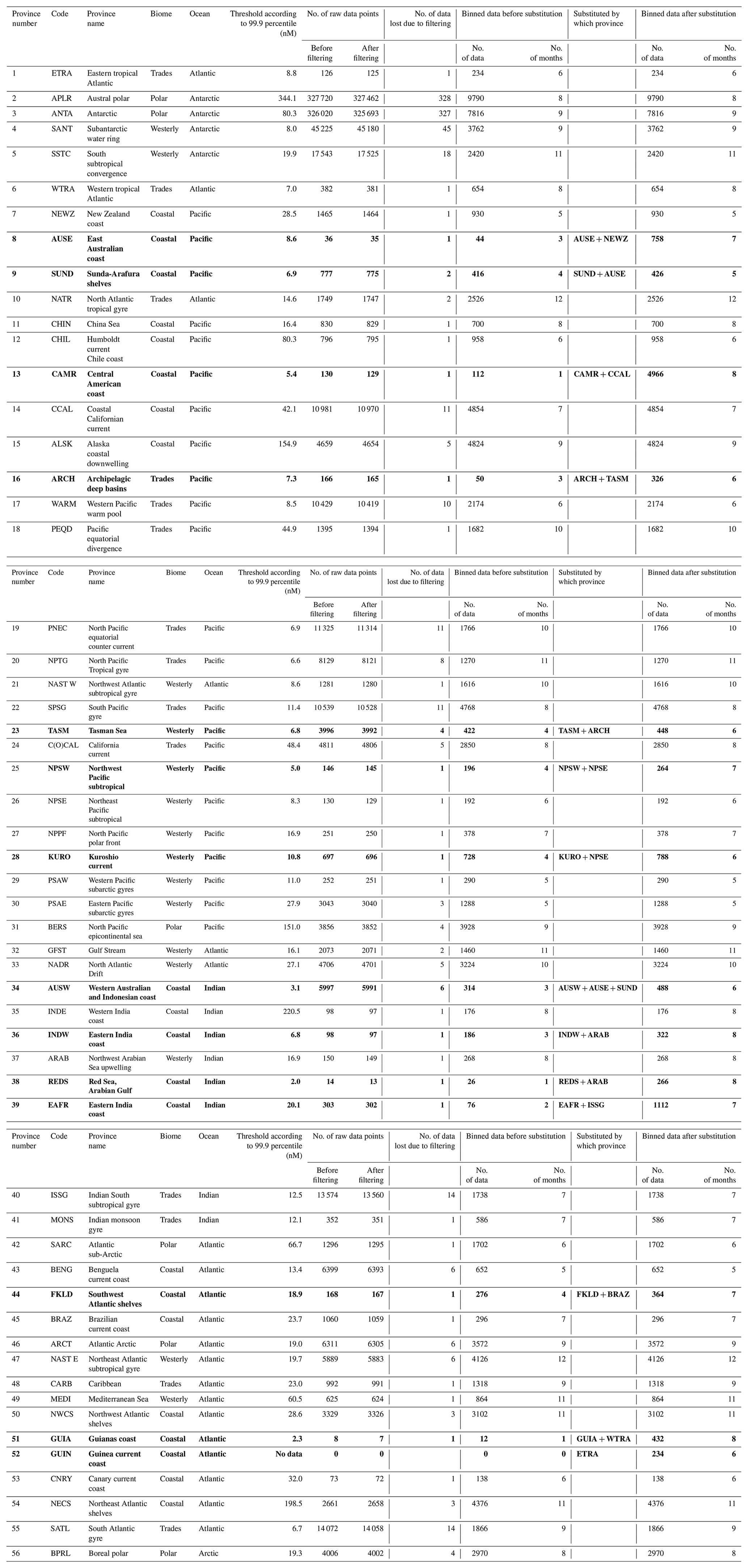
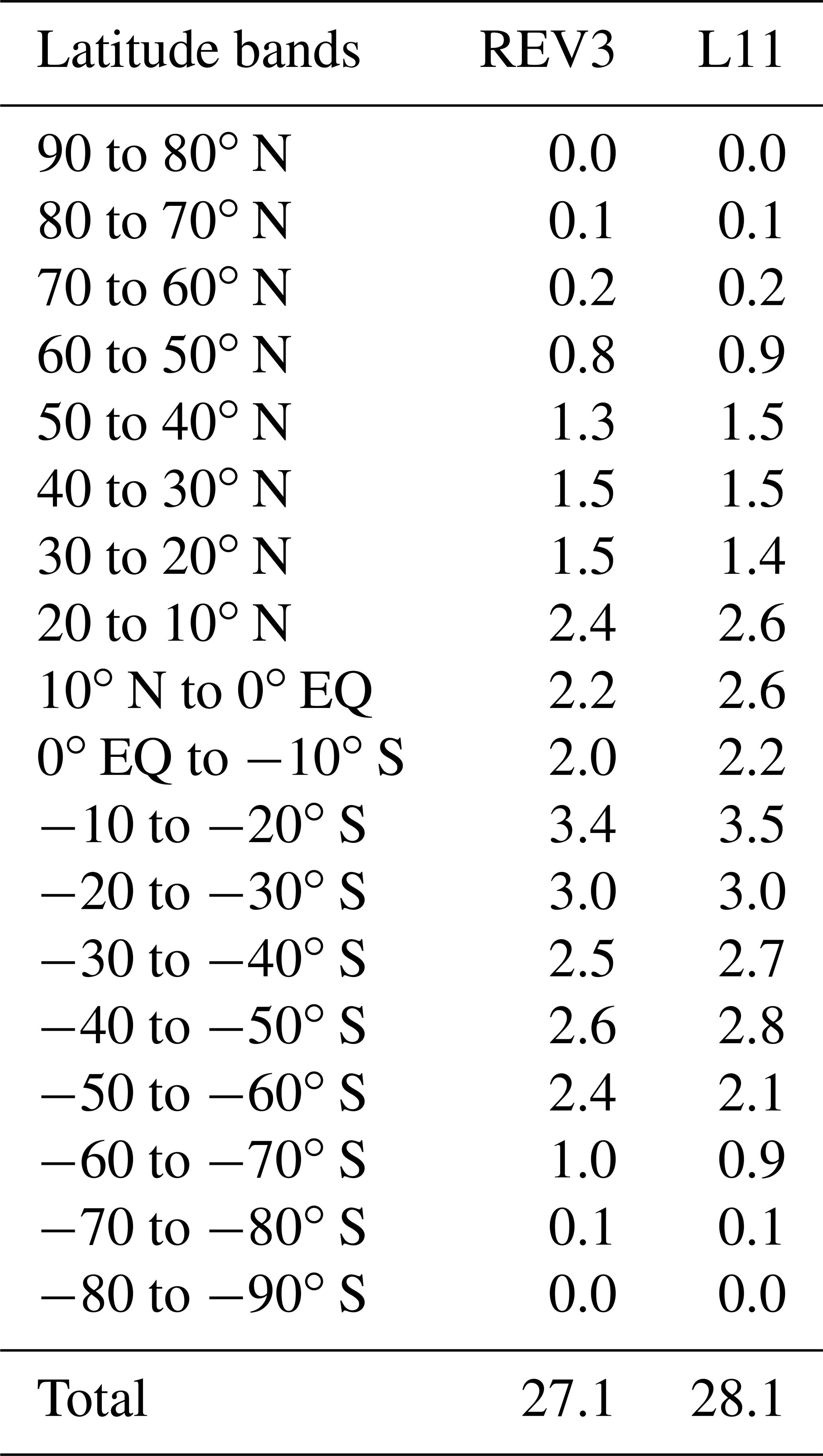
Table 2 Annual DMS flux (TgS yr⁻¹) per 10^∘ latitudinal band obtained from DMS-Rev3 is given in the table along with the annual DMS flux obtained from L11 for comparison.​​​​​​​

2.2 Data unification (spatial and temporal)

The consolidated data contain observations made using vastly different measurement techniques. Until 2000, the GC-based instruments were widely used for the measurement of DMS, but later, high-frequency instruments based on high-resolution mass spectrometry (such as the Chemical Ionization Mass Spectrometer (CIMS) and the Membrane Inlet Mass Spectrometer (MIMS)) started to become more common. This resulted in data with different spatial and temporal resolutions. We analyzed the sampling frequency of the observations (Fig. 2a) to identify the most common sampling frequency. It was found to be greater than or equal to 24 h when all the campaigns were considered. However, this is mostly because older campaigns reported data once a day or less frequently. All more recent campaigns have a much higher sampling frequency, at times as frequent as a data point every second. The high-resolution data collected using the mass spectrometry techniques contributed up to ∼ 59 % of the raw global database. However, the high-resolution data represent only 15 % of the campaigns (Fig. 2b and c). The climatology, which works on averages, can thus become biased towards the data procured using high-resolution instruments. Hence, to avoid this bias and standardize the interpolation field to facilitate further analysis, we binned all the data to frequencies of 1 min, 1 h, and 1 d. After binning the data per minute, around 516 506 data points remain of which about 326 664 points belong only to higher-resolution datasets. This would result in a highly biased input dataset. Daily binning results in 7874 data points, significantly reducing the number of points available for further analysis. Hence, we binned the input data into hourly results, as it helped to degrade the high temporal resolution data to the same resolution as the rest of the historical data. This resulted in a unified dataset of 48 898 data points for DMS-Rev3, reducing bias towards a particular measurement technique or campaign while ensuring that enough data points are available in all the provinces for further analysis. Although keeping a higher temporal resolution would result in more data points, this calculation also helps reduce the disparity in the spatial resolution of the dataset, with the average distance between two consecutive data points for a single campaign coming to about 0.2^∘ (assuming a constant ship speed of 10 knots). In certain regions of the oceans, where the data availability is higher, a high-resolution climatology of up to 0.2^∘ spatial resolution could be attempted, but the majority of the world's oceans are under-sampled or moderately sampled and hence a coarser resolution results in a more realistic climatology. Additionally, since most of the climate models also work on 1^∘ spatial resolution or lower, this dataset was used to create a 1^∘ climatology like that produced earlier in K99 and L11. We tested the sensitivity of the climatology to the temporal resolution. While the global mean did not change significantly depending on whether we used the minute, hour or daily binned data, the minute binned data resulted in regional means biased towards single campaigns in regions where high-resolution data are available.

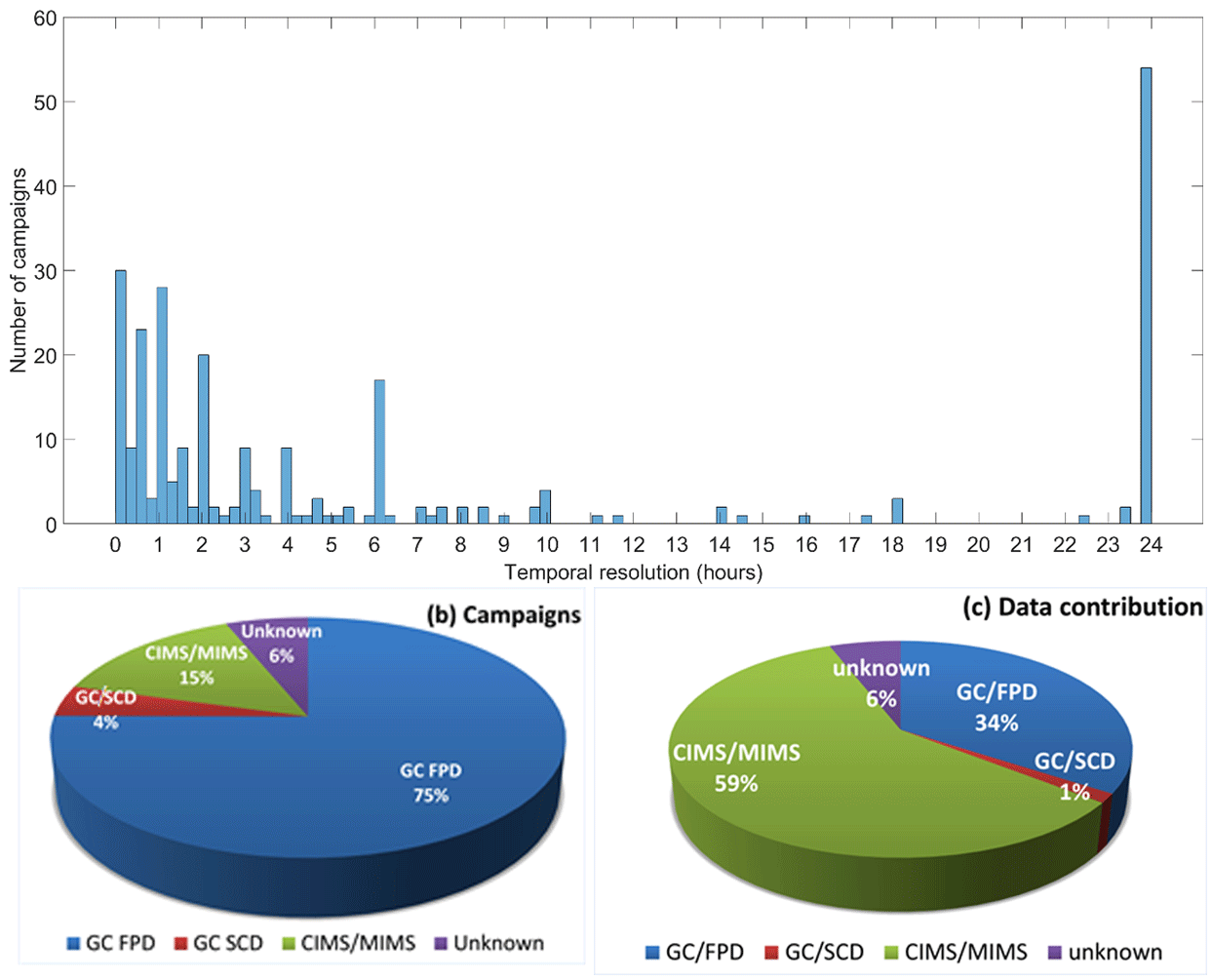
Figure 2 (a) Frequency distribution of the sampling interval for the campaigns included in this study are shown. Note that the “24 h” bin represents temporal resolution lower than or equal to 24 h. (b) The type of measurement technique used to measure DMS during the individual campaigns. The unknown dataset/campaigns resemble the frequency of a GC instrument. (c) The number of raw data points according to the measurement technique is shown. The number of data is dominated by CIMS/MIMS based measurements, but the number of campaigns is dominated by the GC measurements.

2.3 A first-guess monthly climatology according to dynamic Longhurst provinces

Since the data were not uniformly distributed across the oceans, the strategy adopted by the earlier K99 and L11 climatologies was to segregate the data in different provinces based on their biogeochemical properties (chlorophyll-a concentrations, nitrate concentration, salinity, etc.) as defined by Longhurst (2007)​​​​​​​ (Fig. S2a). Computing mean values representing these provinces helped in creating a first-guess global distribution, which is the first step towards a climatology at a coarse resolution. However, satellite images for the biogeochemical parameters reveal that these features are highly dynamic in terms of geographical extents (Devred et al., 2007; Oliver and Irwin, 2008; Reygondeau et al., 2013). Hence, using a static province approach for the whole year (as in K99 and L11), though practical, has an inherent drawback of not accounting for the spatial/temporal changes in the biogeochemistry. This affects the estimations of DMS, especially along the borders of the provinces where static boundaries were used in K99 and L11. To address this, we make use of the dynamic Longhurst provinces based on the work of Reygondeau et al. (2013), who defined the dynamic boundaries based on satellite data between 1997–2007 (Fig. S2b). The monthly data were segregated according to the changing geographical extents for all the provinces and the means of these separated data were used for creating the first-guess fields (Fig. S3). The advantage of using dynamic biogeochemical provinces is that they helped to resolve the environmental, biogeochemical dynamics better on a regional scale, especially in different seasons. The difference due to the inclusion of the seasonal variation in the province boundaries is discussed further in Sect. 3.2.

The DMS-Rev3 also provides an option to create first-guess fields using medians instead of means across the provinces. The median is not affected by the skewed dataset due to a few larger values. The median will also minimize the effect of the blooms that drive high DMS emissions. This approach thus helps to recreate background values better than using means, but can lead to an overall underestimation in regions where blooms are more common, but observations have not been made frequently enough to capture them. Keeping this in mind, we used the province means for the calculation of the climatology, although the values using medians are also reported.

2.4 Data substitution, merging and interpolation

The number of data points available per province differs greatly depending on the sampling carried out in that region during a particular month. Since these are in situ observations, some regions are adequately sampled, some are moderately sampled, while some are rarely or never sampled due to physical constraints like accessibility and remoteness. This results in an uneven distribution of data in the different provinces with respect to space and time. After segregation, some provinces had data for all 12 months of the year, while others had as little as 1–2 months of data (Fig. 3; Table 1). Hence, there was a need to fill the monthly gaps in some of the provinces with data from an appropriate “donor” province to provide sufficient data for a valid interpolation for the annual variation in each province. Across all the provinces, it was seen that for provinces with only 1–2 months with data, substitution from (or merging with, in case the receiving province had no data at all) a single province would result in 5 months with data, providing enough data for interpolation. Hence, if a province had data for less than 5 months, it was selected for substitution/merging, thus all the “receiver” provinces had at least 5 months with data after substitution/merging. The data from the donor province were normalized by scaling up or down based on the ratio of concentrations of the donor and receiver provinces for the common months. In case the receiving province had no data at all, the data were substituted from the donor province. Details of the biogeochemical provinces that were substituted or merged are given in Table 1.

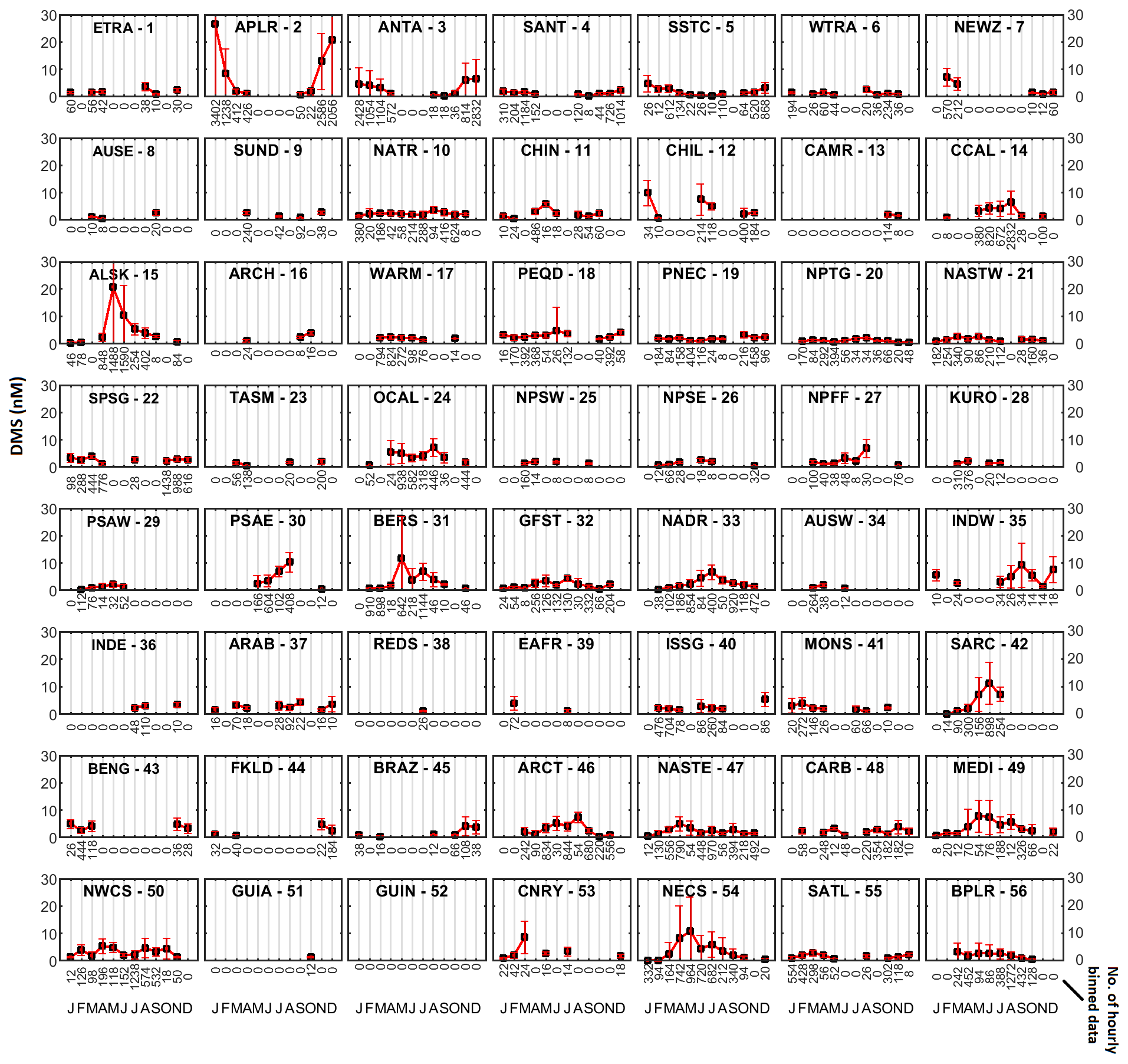
Figure 3 The data distribution in different biogeochemical provinces is different owing to the time, location, and frequency of observation. The black squares represent the monthly mean of data with standard deviations shown as error bars. The number of hourly binned observations in a month is shown below the x-axis.

In all, 14 provinces that needed substitution or merging, i.e., provinces with less than 5 months that contained data, were identified. The provinces off the eastern coast of Australia (TASM and the ARCH) were inter-substituted between each other. The coastal province, AUSE was used to fill the northern coastal province SUND. Although south of New Zealand, NEWZ was also updated with the data from AUSE due to biogeochemical similarities with AUSE. The data from AUSW, AUSE and SUND were merged to complete AUSW. In the northern Pacific, NPSW and KURO were merged with NPSE. In equatorial regions, the coastal province on the east American coast, CAMR was substituted by CCAL following K99 and L11. The province FKLD received data from the adjacent coastal province BRAZ. The coastal Atlantic provinces GUIN and GUIA were substituted by the adjacent provinces ETRA and WTRA, respectively, following L11. Due to the usage of dynamic provinces, the province GUIN is present only in November, December, January, and June. The Canary coastal current seems to highly influence the region occupied by GUIN province converting it to CNRY for the rest of the months. The Indian Ocean coastal provinces INDE, REDS, and EAFR are under-sampled despite the importance for the highly populated South Asian region's respective countries. Data from the ARAB province are merged in the INDE and REDS provinces, while EAFR is merged with data from ISSG.

The substitution or merging was done to ensure that the dependence on interpolation to estimate the values for the remaining months was as low as possible. However, even after this step, it was obvious that the data required some amount of interpolation as only two provinces had data for all 12 months (NATR and NASTE), while other provinces had data between 11 to 5 months (Fig. 3). Hence, to obtain monthly data for each province to estimate the month-to-month variability, it was interpolated to estimate the missing monthly data following the recommendations of Lana et al. (2011). The above ensured that month-to-month variability was created for every province (Fig. 4).

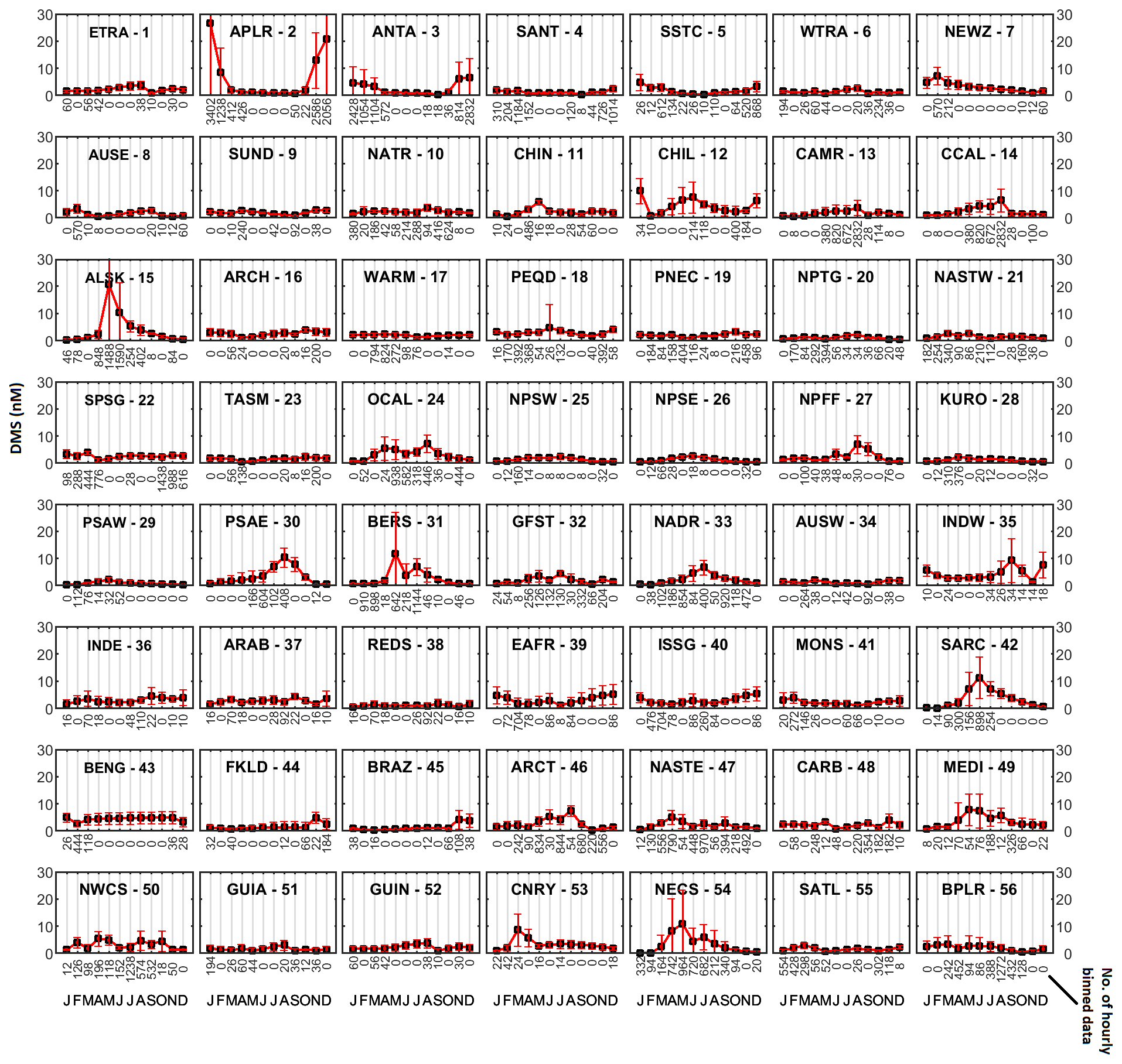
Figure 4 The substituted and interpolated monthly mean data (black squares) with respective standard deviations for each province are shown. The number of hourly binned observations in a month is shown below the x-axis, where 0 indicates that the data were interpolated.

2.5 Incorporation of observed VLS for smoothing

The first-guess database has a uniform distribution within a province as it is the mean value in the province. It also has a sharp and unrealistic transition at the boundaries. Hence, to create a realistic distribution of DMS values at the boundaries, a Shuman filter, which is an unweighted 11-point smoothing filter (Shuman, 1957) was employed. On top of these smoothed first-guess fields, a 1^∘ × 1^∘ spatially binned DMS concentration field was superimposed by replacing the pixels where spatially binned data are available. This replicates the differences in the DMS concentrations within the individual biogeochemical provinces. The average DMS values in a particular pixel (1^∘ × 1^∘) contribute to the value of the pixel. However, there will be an influence of surrounding pixels on each of the pixels. This was accounted for using the Barnes filter (Barnes, 1964), which is a convergent weighted-average interpolation scheme where the radius of influence (ROI, which is the average distance between a grid point and the data points that it influences) is used as a “weight”. The ROI used by K99 and L11 was 555 km (∼ 5^∘, close to the Rossby radius in the tropics). The main aim of using such a filter is to ensure that the DMS variability is captured in the climatology, but this also causes patchiness in the resultant climatology. We tested the sensitivity of the algorithm to the ROI value, different fixed values of ROI: 555, 100, 75, 50, 25, 10, and 7.5 km. On a global scale, each ROI resulted in a different global mean, but once the ROI dropped below 25 km, the mean value stabilized at ∼ 2.44 nM (Fig. S4). Although the global mean did not change by much, large regional differences were observed, with smaller ROI values showing less patchiness in the resultant climatology, indicating that choosing an appropriate ROI is crucial for an accurate estimation of the DMS distribution.

The L11 climatology used the 555 km value since little information was available on DMS variability length scales (VLS) in the oceans, which is the distance over which one would expect the DMS concentration to significantly change as one moves over the ocean surface. However, more recent studies based on high-frequency measurements (Asher et al., 2011; Royer et al., 2015) have been able to quantify the variability in DMS and show that it occurs at a much smaller scale in the order of 15 to 50 km. These findings are consistent with initial findings from a new global VLS analysis of seawater DMS (using data from 2004–2019), which follows the method of Hales and Takahashi (2004) to give a global mean DMS VLS of ∼ 17 km (Fig. S5). The DMS-Rev3 climatology uses VLS results from 11 biogeochemical provinces to estimate the DMS VLS in other provinces and to create a simple DMS VLS distribution map. Monthly geographical variability in VLS was estimated within the dynamic province boundaries, after applying a Shuman filter as detailed above (Fig. 5). Monthly VLS distribution was then used for computing the convergent weighted-average interpolation for DMS using the Barnes filter. The difference in the resultant DMS climatology due to the inclusion of the VLS information is discussed further in Sect. 3.3.

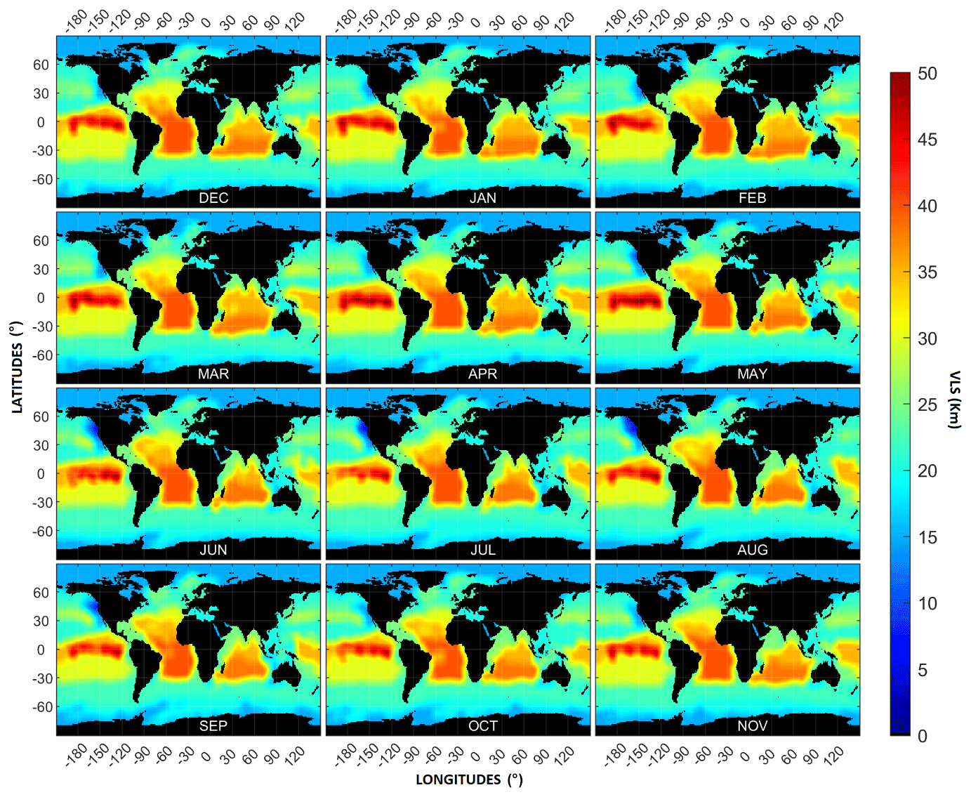
Figure 5 The DMS variability length scales (VLS) used for the weighted-average interpolation computation is shown. The VLS in 11 provinces was based on past observations, and the VLS in the other provinces was estimated by looking for biogeochemical similarities.

2.6 Using sea-ice cover masks

In addition to the oceanic sources of DMS, the presence of sea ice affects the emissions of DMS. The contribution of sea ice to the total DMS production during the melt period was simulated by Hayashida et al (2017) and showed episodic spikes of up to 8 µmol m⁻² d⁻¹. However, the exact extent of this contribution is not known due to the scarcity of field measurements. Further model simulations highlighted the importance of addressing the sea-ice ecosystem separately for better DMS flux estimates. The K99 and L11 DMS climatologies applied a sea-ice filter to mask out any emissions from areas covered with sea ice, which most likely underestimates the total DMS flux.

Considering that large portions of the polar waters can be under sea ice at different times during the year, it is necessary to apply a sea-ice filter to modulate emissions in these regions. This can be done in two ways: (i) before creating the DMS climatology to filter out data that are under sea-ice regions; or (ii) after the climatology is created as a mask. A sea-ice monthly climatology (Fig. S6) was created using data obtained from the Defense Meteorological Satellite Program, F13 Special Sensor Microwave/Imager (SSM/I), and Scanning Multichannel Microwave Radiometer (SMMR). The DMS-Rev3 code replaces the data with zeros when considered to be under sea ice, where sea ice is less than or equal to the set threshold. For example, the Antarctic coastal region is a DMS hotspot during the southern hemisphere summer and is a sea-ice covered region during the winter with no DMS emissions. An annual average ignoring these regions during winter would result in a hotspot with the annual average biased towards the summer values.

A sea-ice threshold cutoff value of 50 % was used (which can be changed in the code). If the filter was applied after data unification, but before the creation of the climatology, the mask removed only 17 data points (88 data points for 30 % sea-ice cover threshold) from the 48 898 data points that are deemed to be under the sea ice. This does not lead to a significant change in the overall calculations. However, if the mask is applied after the creation of the climatology, large portions from the polar provinces come under the mask and lead to changes in the monthly and the annual global mean values (detailed in Sect. 3.4).

2.7 Sea–air DMS flux estimations

The sea–air DMS flux was estimated using the output of DMS-Rev3 to understand the impact of the new climatology. The estimations were carried out following the same procedure as Lana et al. (2011) which used the Nightingale et al. (2000) parameterization. This parameterization is based on the DMS gas transfer velocity utilizing the wind speed at 10 m and the climatological sea surface temperature (SST). The inputs for calculating the flux were for the same period as that used for L11 (1978–2008) and were obtained from the NCEP/NCAR reanalysis project (http://www.esrl.noaa.gov/, last access: 5 July 2021). This was necessary for a one-to-one comparison of DMS-Rev3 and L11 flux estimations.

2.8 Uncertainties in the climatology

Estimating the uncertainty in the climatology is difficult due to the variety of methodologies and the lack of reported observational uncertainties for most of the campaigns. The uncertainties in the DMS climatology were hence estimated from the point of data unification (Sect. 2.2) and will therefore be an underestimate of the total uncertainty in the final climatology. First, the standard deviations were computed for the hourly binned observations. This standard deviation was further propagated while spatially averaging the data when creating the 1^∘ × 1^∘ bins. An additional standard deviation was computed for the first-guess fields, which use the means across the biogeochemical provinces (Sect. 2.3). These standard deviations from the hourly binned data, pixel binned data and province binned data were then propagated through the calculation of pooled standard deviations. The uncertainty introduced due to the smoothing using the Shuman and Barnes filters (Sect. 2.5) is difficult to estimate, and hence the same smoothing filters were also applied to the standard deviations to create a monthly and annual uncertainty database corresponding to the DMS concentrations. While these uncertainties are not a complete estimation of the errors, they provide an estimate of the range of DMS concentrations in the climatology. The calculated global monthly and annual standard deviations are shown in Fig. S7.

3 Results and discussion

3.1 Features in DMS-Rev3

3.1.1 Global

Figure 6 shows the monthly and annual climatological distribution of surface seawater DMS concentrations as estimated by the DMS-Rev3 algorithm after the application of a 50 % sea-ice cover mask (the distribution without the application of the sea-ice mask is shown in Fig. S8). For the annual mean climatology, the DMS concentrations range between 0.1 to 7 nM, of which ∼ 85 % of the grid points contain DMS concentrations below 3 nM (Fig. S9). When globally averaged across all the oceans, DMS-Rev3 estimates the annual mean at 2.26 nM (2.39 nM with no sea-ice mask – henceforth nM^* indicates values without a sea-ice mask). If province medians are considered instead of the province means, the global annual average concentration reduces to 1.79 nM (1.73 nM^*), about ∼ 26 % lower than the L11 climatology (∼ 21 % lower than DMS-Rev3 calculated using means). The highest global averages are observed in November, December, January, and February with average values of 2.51 nM (2.85 nM^*), 3.17 nM (3.46 nM^*), 3.32 nM (3.57 nM^*) and 2.48 nM (2.67 nM^*), respectively (Fig. S10). The higher values in these months are mainly due to large concentrations in the southern hemisphere with coastal Antarctica dominating the peak values. The global mean annual cycle shows a clear peak in December and January, followed by the first minimum in April ∼ 2.19 nM (∼ 2.07 nM^*). The values then show a modest increase through the months of May–August (with values around ∼ 2.15 nM) due to the northern hemispheric summer. This can be attributed to the higher DMS values in the northern high latitudes. September shows the second minimum lowest mean DMS values of 1.72 nM (1.56 nM^*). The region south of 60^∘ S has the highest average concentrations, with large peaks seen in the high productivity regions such as the Weddell Sea and the Ross Sea. Outside this polar environment, higher values are seen on the southwest coast of Africa and the west coast of South America. Elevated concentrations are also observed in the Mediterranean Sea and the Arctic Ocean close to Norway and Greenland. The waters close to Alaska and California also show higher than the global mean concentrations.

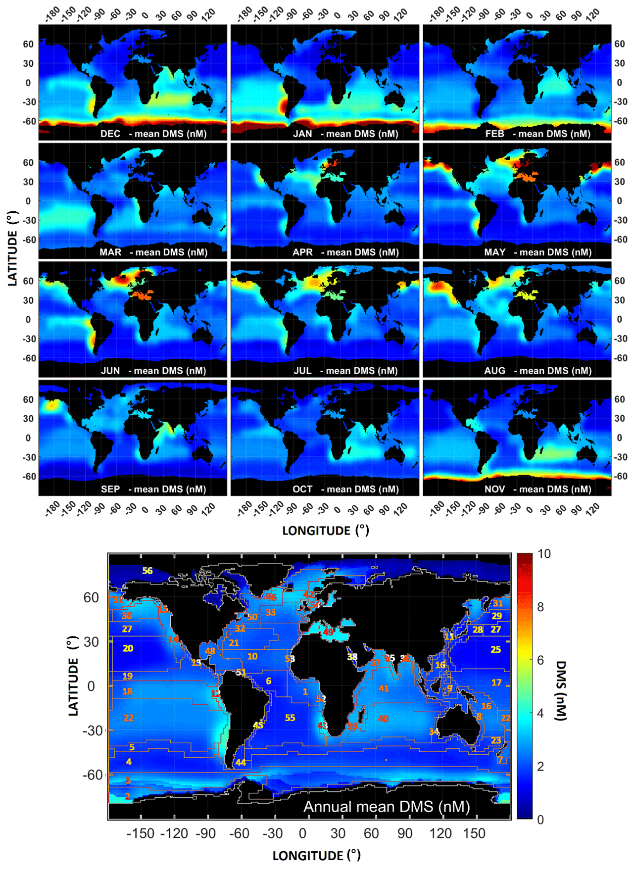
Figure 6 Distribution of the monthly and annual DMS concentrations as estimated by DMS-Rev3 climatology with a 50 % sea-ice mask.

A clear regional annual cycle is observed in most locations, with the southern and northern hemispheres peaking during their respective summers. The range of values also differs according to the months, but higher values of as much as ∼ 8.8 to 14.7 nM (10–15.1 nM^*) are seen in the Antarctic coastal province (APLR), especially in November, December, and January. However, even during these months, more than ∼ 60 % (83 % in November) of the grid points contain concentrations below 3 nM (Fig. S9). The final output for individual provinces is shown in Fig. S11.

3.1.2 Polar

Regionally, the highest values were found in the polar biomes during their respective summers (60^∘ to 90^∘ both in the northern and southern hemispheres). The APLR showed the highest levels of DMS with peak monthly averaged concentrations of 12.83 nM (13.34 nM^*) and 14.72 nM (15.16 nM^*) in December and January, respectively (Fig. S11). The DMS concentration was 0.58 nM in September. However, since the region is under the ice during this season, this value corresponds to the concentration limited to a smaller region to the north of the Weddell Sea, which stays exposed and out of ice cover (Fig. 6). The concentrations increase through spring and summer until January, after which the values decrease to April which has an average of 1.22 nM (1.23 nM^*). Over these months, since most of the APLR province is under sea ice, it does not make a large contribution to the global monthly mean DMS. Similarly, most of the polar province of BPLR also gets masked by sea ice during the northern winter. The peak DMS concentration was 4.31 nM (2.92 nM^*) during May (Fig. S11). In the North Atlantic region, phytoplankton blooms dominate the Labrador and the Grand Banks coastal regions (ARCT province) in spring and summer (Friedland et al., 2016), driving high DMS concentrations. A similar peak is observed in the SARC province with elevated DMS values during the same seasons (Fig. S11).

3.1.3 Extra-tropics

The southern extratropical region gets split into three sectors: the Indian Ocean sector, the Atlantic Ocean sector, and the Pacific Ocean sector. The northern extra-tropical region has two sectors: the Pacific Ocean and the Atlantic Ocean.

In the southern hemisphere, in the Indian Ocean extra-tropical region, the monthly variation observed in the polar province APLR is also noticed in the adjacent province ANTA, which shows peak monthly mean concentrations of 7.76 nM (8.32 nM^*) in December and 7.56 nM (7.69 nM^*) in January (Fig. S11). The adjacent provinces, SANT and SSTC, form a part of all the sectors mentioned above, although divided by the South American and the African continents. These provinces follow a similar annual variability as the APLR and ANTA provinces, although the peak values are lower (Fig. S11). These concentrations reflect the summertime productivity of the Southern Ocean during summer. The province ISSG in the Indian Ocean sector, spread over the tropics and extra-tropics, follows a similar seasonal trend, although being further away from the polar region, it has much lower month-to-month variations. The highest concentrations are observed in the months of November–December–January. During the rest of the year, the values are lower and stay close to ∼ 2.2 nM, with a slight increase in June to 2.59 nM (Fig. S11). The province to the west of ISSG (EAFR) also has a similar annual trend with similar concentrations to those observed in the ISSG province. The slightly higher concentration in June in these two provinces is attributed to winter blooms occurring off the Madagascar coast (Dilmahamod et al., 2019). This trend is different in the AUSW province (east of ISSG), where the values are also higher during November (2.46 nM), December (3.19 nM), and January (3.24 nM), but a clear low is observed during August (1.05 nM) (Fig. S11).

In the southern hemispheric Atlantic Ocean sector, the provinces SATL, FKLD, BRAZ and BENG are a part of the South Atlantic Gyre. The mean values in these provinces decrease from approximately 2 nM in January to less than 1 nM in May (Fig. S11). The African coastal province, BENG shows higher values in January (4.09 nM) and March (3.59 nM) with lower concentrations in February (2.54 nM). This province does not show significant variation throughout the year owing to the continual supply of nutrient-rich water due to an upwelling that supports primary production and hence DMS production (Jury and Brundrit, 1992) (Fig. S11).

In the southern hemispheric Pacific Ocean sector, the provinces AUSE, TASM and NEWZ cover the eastern and southern coastal region of Australia and coastal New Zealand. The primary production in TASM and NEWZ shows an annual cycle controlled by the availability of solar radiation, wind stress and MLD similar to most provinces, but the variation is large for these variables (Chiswell et al., 2013). Variability in the DMS concentrations follows variability in chlorophyll and sunlight with the highest concentrations observed in summer, reducing in autumn with a decreasing trend until the summer of the following year. The SSTC DMS concentrations are constant throughout the year, although from July to October DMS levels are consistently lower. This is most likely due to the autumn, winter and spring phytoplankton blooms observed in the TASM and NEWZ regions (Chiswell et al., 2013) (Fig. S11).

Provinces in the northern extra-tropical regions (BERS, PSAW, PSAE, NECS) typically show higher values in the northern hemispheric summer. The provinces in the North Atlantic extra-tropical gyre (NAST(W), NAST(E), GFST, NWCS, NECS and MEDI) typically show peaks during the northern summer. This pattern results from a combination of plankton seasonal species succession and short-term sunlight effects on DMS budgets, stimulating DMS production, inhibiting bacterial consumption, enhancing photolysis, etc. (Galí and Simó, 2015). The provinces NECS and MEDI show a similar trend to the polar province SARC. In addition to the summer peaks, an additional peak is also observed during the northern spring that has higher values than the peak in summer. The trends in the NECS province appear to be dominated by the spring blooms of the Baltic and the North Sea (April = 6.71 nM; May = 8.55 nM). A second bloom driven by dinoflagellates has been reported to occur in July (Hjerne et al., 2019) and coincides with a second peak in the DMS concentrations at 5.98 nM. The GFST and NWCS provinces show similar values and trends with twin maxima in spring and summer. Being a coastal province, NWCS shows consistently higher values than the GFST province. These higher values in the North Atlantic provinces are mostly associated with the Phaeocystis pouchetii and coccolithophores blooms occurring in the months of May–July (Iida et al., 2002; Matrai et al., 2007; Matrai and Keller, 1993) (Figs. S11 and 6).

In the Pacific region, the BERS, PSAW, and PSAE provinces show higher values during May followed by lower concentrations in June and the concentrations rise again in July. A gradual decrease follows the summer peak, and the lowest values are observed during winter in December–January. In the Bering Sea and adjacent regions, blooms tend to form due to the dynamics of sea-ice retreat in spring (Jin et al., 2007; Sigler et al., 2014). This most likely contributes to the maxima observed in the respective provinces. Although significant blooms were also reported in autumn (Ardyna et al., 2014), the magnitude of increase in the DMS concentrations is smaller after more data have been added.

3.1.4 Tropics

In the Indian Ocean sector of the tropics, the province MONS is in the central Indian Ocean with coastal provinces of REDS, INDW and INDE to the north, ARAB to the west, AUSW to the east, and ISSG to the south. The annual variation in the MONS province is like the ISSG province, although with the peak value observed in February instead of December (3.66 nM). The INDE and REDS provinces show a similar monthly variation as the ARAB province. This region experiences the southwest and northeast monsoons during the periods between June–September and October–December. The Somali current flowing through the ARAB and INDE provinces is characterized by seasonal changes influenced by the southwest and northeast monsoons. During June–September, the warm southwest monsoon moves the coastal waters north-eastward, creating a coastal upwelling (McCreary et al., 1996). This could be a reason for the higher mean DMS concentrations observed in these provinces during June and July (∼ 2.8 nM). However, these variations in DMS are not observed in the INDW province which is on the eastern coast of the Indian peninsula and not directly affected by the upwelling. In November, the coastal Indian province INDW shows higher values than the ARAB province, most likely due to the northeast monsoon winds increasing continental aerosol deposition over the ocean surface, thereby increasing productivity due to increased nutrient availability (Figs. S11 and 6).

In the northern tropical Pacific Ocean, the province NPTG shows higher values in August (2.34 nM), while the lowest levels are observed in January (∼ 1 nM). DMS concentrations increase from a low in January to 1.61 nM in April, decreasing slightly to 1.29 nM in May and increasing thereafter until August. In PNEC, there is no significant annual trend as the mean DMS concentrations stay in the 2–2.6 nM range with one lower value in May (1.59 nM). From May to August, PNEC and NTPG show an increase in DMS (Figs. S11 and 6).

In the southern tropical Pacific region, the provinces SPSG, CHIL, PEQD, and PNEC are seen to have little variability unlike those seen in the Indian Ocean. The mean DMS values in the SPSG province are higher in January and March (∼ 3.3 nM), with a drop in February to 2.63 nM. The mean then drops to 1.39 nM in April followed by an increase to 2.74 nM in July. From June onwards, the mean DMS concentrations are ∼ 2.6 nM (2.34 to 2.9 nM) up until December (2.9 nM). During the southern summer months, CHIL is influenced by increased DMS production with higher mean concentrations in December (4.93 nM) and January (7.53 nM). This is also observed in the PEQD province as the mean DMS is slightly higher in December (3.38 nM) and January (3.14 nM) compared to the other months. The Chile coastal “Humboldt” current is one of the most productive currents (Penven et al., 2005), and this may be driving the higher DMS concentrations during May–June (May = 4.27 nM, June = 5.61 nM) in CHIL. Since the current flows northward from CHIL to the province PEQD, the effect is seen as a slight increase during June (3.35 nM) in PEQD (Figs. S11 and 6).

The Atlantic Ocean tropical sector is comprised of the provinces CARB, NATR, CNRY, ETRA, WTRA, GUIN, GUIA, and SATL. The major gyres in the northern and southern tropics are NATR and SATL. The gyres show elevated DMS concentrations during August (NATR) and March (SATL). However, in the SATL province, the peak concentration is observed during the transition from summer to autumn (March = 2.64 nM). In the SATL province, the open ocean sees the confluence of the Brazilian–Malvinas current which significantly affects the productivity of the region. During most months, DMS concentrations are in the range of 1–2.5 nM in this province, with the lowest observed in May (0.83 nM). The NATR province has higher values throughout the year compared to SATL, except in March. In the ETRA and WTRA provinces, a clear annual peak is seen in August, which coincides with the maximum extent and magnitude of phytoplankton blooms (July–September) in the eastern equatorial Atlantic Ocean (Pérez et al., 2005). The inputs from the Amazon and Congo rivers are a major source of nutrients in this area throughout the year, with peak input between May and September. Similarly, in the GUIA and the CARB provinces, the Amazon and the Orinoco river inputs influence the seasonal variability of primary production (Forget et al., 2011). This is seen in the peak concentrations of DMS in CARB (September = 2.74 nM) and GUIA (August = 2.75 nM). In the eastern Atlantic, the GUIN province shows a seasonal presence, with the CNRY province occupying its location as seen in the dynamic biogeochemical province map (Figs. S1, S11). Three characteristic peaks are seen in the CNRY province in March (3.86 nM), August (3.34 nM) and November (2.45 nM) (Figs. S11 and 6).

3.2 Differences due to usage of dynamic biogeochemical province boundaries

Dynamic biogeochemical province boundaries as defined by Reygondeau et al. (2013) were used in the DMS-Rev3 climatology instead of static boundaries to incorporate the monthly variability of surface properties in the world's oceans. In this section, we describe the differences caused by using the dynamic province boundaries as compared to the static boundaries (Figs. 7 and S12a). As expected, most of the differences are seen at the province boundaries when compared to the output using static provinces. Major differences are seen in the polar regions and smaller differences in the extra-tropical and tropical oceans. When globally averaged, the annual difference caused in the climatology by using the dynamic province boundaries is only about 0.02 nM (∼ 5.1 %) (Table S1), however, regional differences are up to ±5 nM (±100 %) (Figs. 7 and S12a).

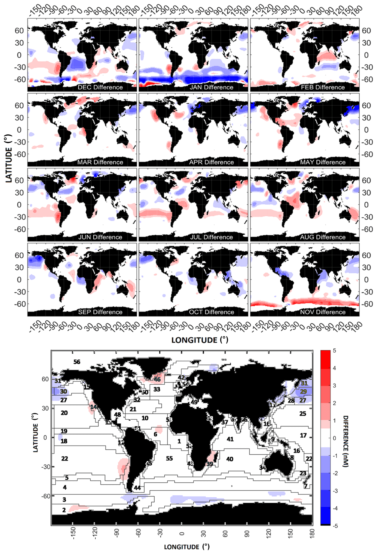
Figure 7 Differences between the monthly and annual mean DMS concentrations estimated using dynamic and static biogeochemical province boundaries (dynamic − static).

The sea-ice mask excludes data from the Arctic region when sea-ice cover exceeds 50 %. If the sea-ice mask is ignored, the use of dynamic provinces generates significant differences in the Arctic Ocean region, with increases of 1–3 nM (+100 %) during February–March and decreases of 1 to 3 nM (−40 % to −60 %) during April (Fig. S12b). The winter and spring months show a positive change in the DMS concentrations as compared to the summer months where a reduction in the DMS concentrations is observed (Fig. 7). The Arctic region, especially the Nordic Seas where ice-free regions exist even during the winter season, showed a positive difference with a maximum of 100 % change during February. The difference stayed positive during the northern winter (∼ 40 % to 60 %), while it ranged from 0 % to $\sim -\mathrm{40}$ % for the northern summer.

The Southern Ocean region showed the greatest regional differences in November where concentrations differed by >4 nM (+100 %), while the largest reduction was observed in January (−4 nM; −50 %). Both large positive and negative differences are seen in this region during the summer months with a negligible difference during the rest of the year.

For the rest of the regions in the extra-tropics and tropics, regional differences of between ±2 nM (up to 100 %) can be seen, changing throughout the year. Most of the world's oceans show differences of ±20 %. Clear patches with larger differences can be observed, such as in the Atlantic Ocean where the differences are around −2 nM (−60 % to −80 %). A few patches are also observed in the northern and equatorial Pacific Ocean, where large differences are seen in different locations depending on the month (Fig. 7). Globally, the largest difference is seen during November, where the use of dynamical province boundaries leads to an increase of 0.36 nM in the globally averaged concentration, while the smallest difference is seen during May (−0.003 nM).

3.3 Differences due to usage of variability length scales (VLS)

The other major change in DMS-Rev3 was the use of DMS VLS, which led to significant changes, reducing the patchiness that was a feature of past climatologies. In this section, we present the effect of using VLS compared to the fixed value of 555 km when applying the Barnes filter (see Sect. 2.5). The differences (DMS_VLS−DMS₅₅₅) are shown in Fig. 8 and the percentage differences ((DMS_VLS−DMS₅₅₅) × $\mathrm{100}/$DMS₅₅₅) are shown in Fig. S13. When globally averaged, the annual DMS concentration increased by 0.025 nM (+7.4 %) when using the VLS while applying the Barnes filter (Table S1). Annually, the largest differences of up to ±4 nM (±90 %) were observed in the coastal Antarctic region and smaller increases were observed in certain regions of the Atlantic and Pacific oceans. However, over most of the world's oceans, the difference was within ±0.3 nM (±5 %).

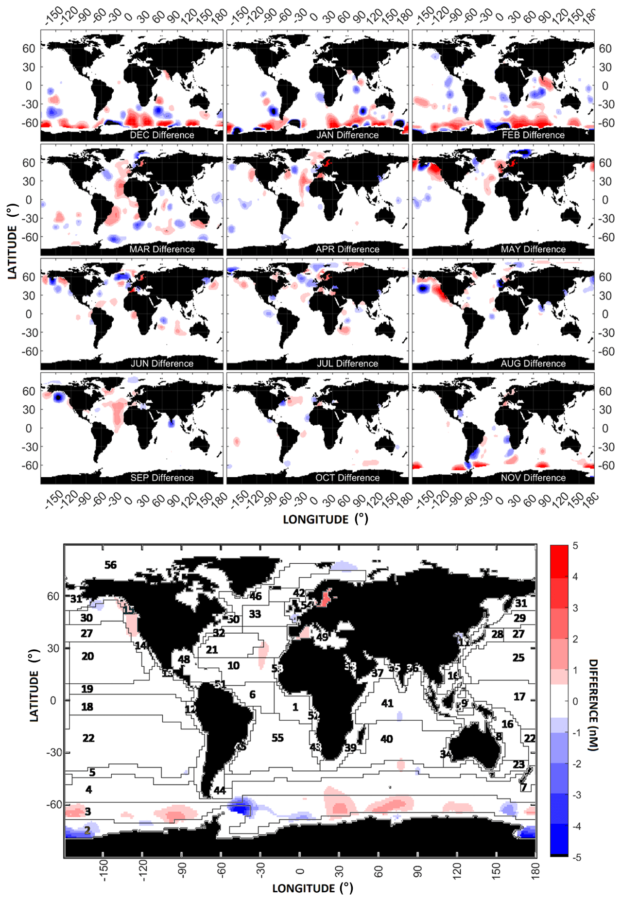
Figure 8 Differences in the DMS concentrations caused using variability length scales (VLS) instead of a fixed value for the radius of influence as used by L11 (555 km) for the weighted average interpolation computation. (VLS – 555 km).

When the monthly differences are considered, large regional differences show up between the VLS and 555 km filters. For instance, during the southern hemispheric summer (December, January, February), large differences of above ±5 nM (±100 %) are seen in the Southern Ocean. This suggests that the use of a fixed value of 555 km led to severe over- and underestimations in this region. During February, the entire Indian Ocean region shows patches of both positive and negative differences. The central Atlantic region also shows positive differences during the months from March to May, with the largest differences observed in March ∼ 2 nM (>100 %). The Pacific Ocean shows the least differences amongst all the world's oceans. The Arctic region also shows differences of above 100 %, especially during the summer season. Overall, the largest differences are observed in the high concentration polar regions, with smaller differences seen close to the tropics.

3.4 Differences due to sea-ice cover

There is a marginal change in the global annual mean DMS (<1%) when applying the sea-ice cover at 50% threshold after the data unification, before creating the DMS-Rev3 climatology. The most noticeable changes are when the filter is applied after the creation of climatology. The global annual DMS reduces from 2.39 to 2.37 nM (0.8 % reduction when using a 95 % sea-ice mask) and further down to 2.21 nM (∼ 8 % reduction when using a 20 % sea-ice mask). The relationship with the sea-ice mask and the averaged annual global DMS concentrations is now shown in Fig. S17. The relationship between the percent threshold sea ice and the DMS concentration is linear, showing that the polar regions contribute heavily to the annual global average.

For this study, a threshold of 50 % was considered for the sea-ice cover. The sea-ice cover removes a major part of the province of BPLR and parts of the BERS, SARC and ARCT provinces were also masked, reducing the monthly means of the respective provinces. Similarly, in the southern region, the province APLR was also masked by the sea ice. The southern hemisphere winter shows the presence of sea ice to a much larger extent, covering areas of APLR and ANTA provinces.

3.5 Differences between DMS-Rev3 and L11

Figure 9 shows the differences between the DMS-Rev3 and L11 climatologies (DMS_REV3−DMS_L11) and Fig. S14 shows the percentage difference ((DMS_REV3−DMS_L11) × $\mathrm{100}/$DMS_L11) between the two. The most noticeable difference is the reduced patchiness in the data distribution. This is mainly due to the improvements made in the interpolation routine and the use of observed DMS VLS in the Barnes filter (Sect. 2.5). For the global annual climatology mean, 73 % of the grid points show a positive difference (Figs. 9, S15), ∼ 51 % data show differences up to ±1 nM (±10 %), and ∼ 81 % of data have differences within ±2 nM (±30 %) (Fig. S15). Only 0.24 % of data show differences equal to or above 100 % (>5 nM). Overall, the DMS-Rev3 climatology estimates a global annual average DMS concentration that is 0.05 nM less than the L11 climatology. The largest mean difference is seen in November (+0.31 nM), and the lowest difference is seen in September (−0.03 nM) (Table S1).

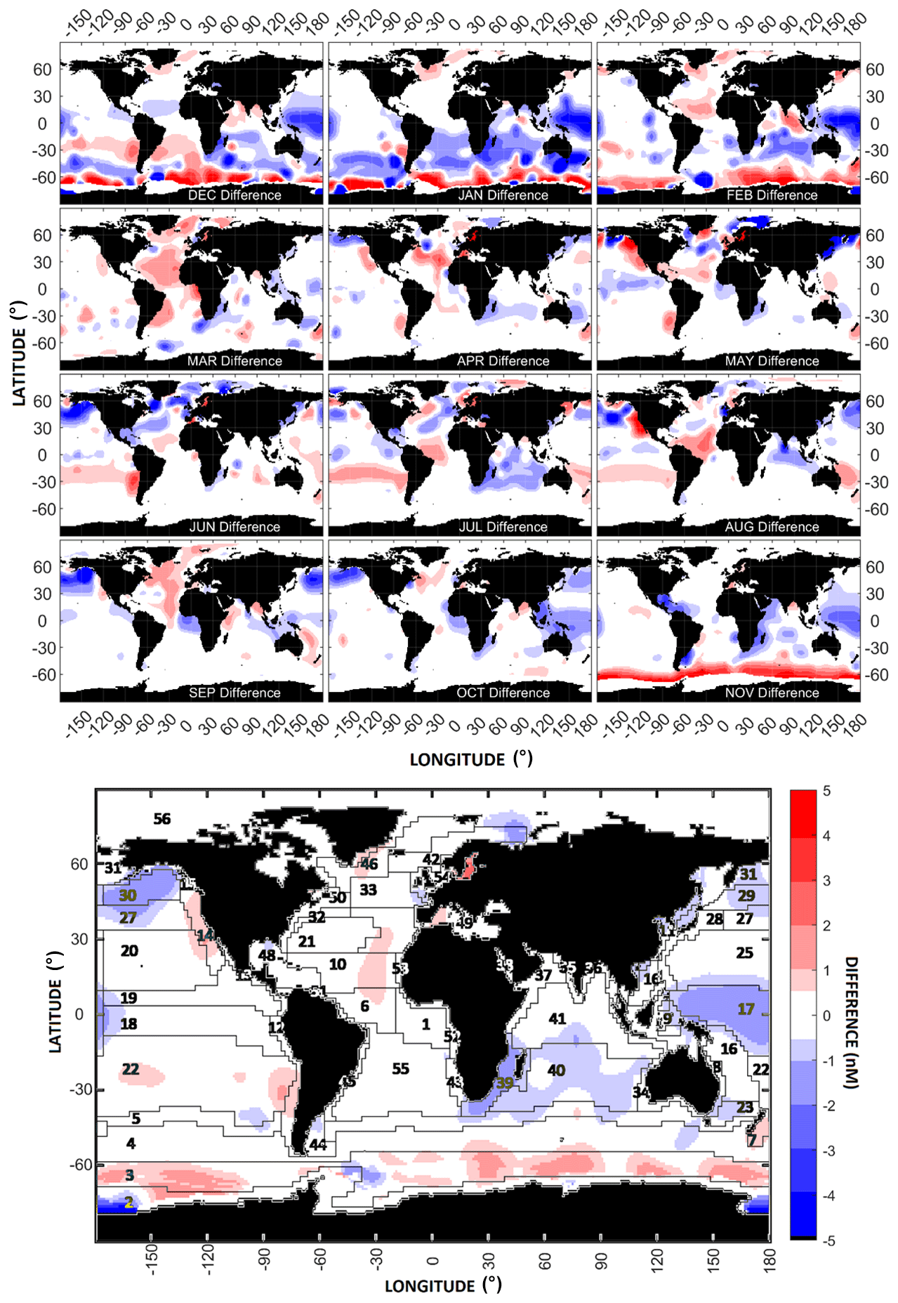
Figure 9 Differences between the monthly and annual mean DMS concentrations of the Rev3 and L11 climatologies (​​​​​​​Rev3 − L11).

Most of the large differences are found in the polar regions, especially in the Southern Ocean. The equatorial oceans show differences less than ±0.5 nM, except in parts of the Indian and Pacific oceans, where differences of up to −1 nM are observed (Fig. 9). The two climatologies agree well in the oligotrophic regions of the oceans where lower DMS concentrations are observed. Monthly, the largest differences are seen in the Southern Ocean during the months of November–February, with the DMS-Rev3 climatology displaying higher values in November throughout the Southern Ocean. For the rest of the southern hemisphere summer, positive and negative differences of up to 5 nM are seen in the Southern Ocean, where the negative differences coincide with the patches that were a feature in the L11 climatology.

4 DMS flux

The global sea–air DMS flux (Fig. 10) reveals that ∼ 93 % of the world oceans emit DMS in the range of 0–10 µmol S m⁻² d⁻¹, with a few hotspots in the world's coastal regions like the provinces of BENG, ARAB, along with oceanic provinces like the confluence of PEQD and SPSG in the Pacific, and the ISSG province in the central Indian Ocean region, which covers ∼ 7 % of oceans with emissions in the range from 10–20 µmol S m⁻² d⁻¹. The Southern Pacific Ocean shows higher values as compared to the Northern Pacific, although the Eastern Pacific shows more flux as compared to the western Pacific, mainly due to the coastal provinces of CHIL, CAMR, CCAL, and ALSK which show particularly large fluxes. The North Atlantic region, mainly in the GFST and NADR, shows a higher flux compared to the South Atlantic. The equatorial Indian Ocean region shows lower values than the rest of the Indian Ocean. The Arabian Sea shows a higher flux of DMS compared to the Bay of Bengal. The total global annual DMS flux is estimated at 27.1 TgS yr⁻¹, about 3.5 % lower than the L11 climatology. The DMS flux variability follows the variability in DMS concentration, which is significant at the regional scale.

Figure 10 Distribution of the monthly and annual DMS flux as estimated by DMS-Rev3​​​​​​​ climatology with 50 % sea-ice mask.

The entire oceanic region to the south of ∼ 30^∘ S seems to be a major source of DMS during the southern hemisphere summer. The northern hemisphere summer shows elevated DMS emissions in only a few regions. Additional regions are visible as hotspots in the open ocean (e.g., in the North Atlantic and Central Indian Ocean) as well as in coastal regions like those observed off the Chile coast, South of Alaskan coast in the Pacific Ocean, and the North-western Arabian Sea. The hotspot observed in the Central Indian Ocean region is present almost through all seasons, although it seems to be weakening during the northern spring. With an annual average of ∼ 2.76 nM, this region is above the global average, increasing the annual DMS flux (∼ 14 µmol S m⁻² d⁻¹).

Since the Nightingale et al. (2000) parameterization uses the wind speed and the SST for estimation of the gas transfer from sea to air, the DMS flux hence calculated shows a direct relationship between the wind speed and SST. However, wind speed is a major driving force of the gas transfer velocity, which is a major determinant of the flux. As observed by Bell et al. (2013) and Zavarsky et al. (2018a), the wind speed of about ∼>10 m s⁻¹ seems to be one of the main factors to suppress the DMS fluxes. The optimum response was observed in the range of 5–8 m s⁻¹ approximately comparing the wind speed climatology and DMS fluxes in the region where the DMS fluxes were found to be higher over the global oceans. This explains most of the regional flux variability as observed in the DMS-Rev3 output. The evidence of this is seen in the Antarctic coastal region, which seems to be a major source of DMS during the southern summer. But due to the higher wind speed over the region, the contribution to the DMS flux is lower than one would expect. This region also has lower SST, which further reduces the gas transfer.

The differences in the fluxes with respect to L11 show a similar pattern to that seen in the distribution of oceanic DMS on monthly and annual scales (Fig. S16). This means that although the change in the global annual average of DMS flux is not substantial, the DMS-Rev3 climatology has large regional changes (Table 2) due to a reduction in the patchiness of the oceanic DMS concentrations. Most of the high latitudes show a reduced flux, while the tropical regions show an enhanced flux.

5 Code and data availability

​​​​​​​The data used for creating the climatology, along with the algorithm, can be found in the online repository: https://doi.org/10.17632/hyn62spny2.1 (Mahajan, 2021).

6 Conclusion

An updated global sea surface DMS concentration climatology was created by upgrading the processing algorithm initiated by Kettle et al. (1999) and Lana et al. (2011), along with the inclusion of new data compiled from various sources. The global annual average concentration reduced to 2.26 nM, although large differences of up to 5 nM were observed on regional scales during certain months. This is an important difference considering the effect of regional emissions on the total impact of DMS on the Earth's radiative budget (Fiddes et al., 2018; Mahajan et al., 2015; Thornhill et al., 2021; Woodhouse et al., 2013). The global sea–air flux of DMS is estimated at 27.1 TgS yr⁻¹ which is similar to L11 (a 3.5 % decrease). The use of dynamic province boundaries allowed the estimation of more realistic annual trends in different regions. The patchiness in the climatology identified in previous estimates was reduced by region-specific data exclusion (Sect. 2.2) and the usage of the observation-based VLS (Sect. 2.5). The use of dynamic province boundaries and VLS was not important at the annual and global scales but resulted in large differences at regional scales. Although this climatology shows significant improvements in the estimation of seawater DMS concentrations, it still suffers from a lack of continuous observations, especially in certain parts of the world's oceans. Focus can be given specifically to the provinces NEWS, AUSE, AUSW, SUND, and ARCH which are present around Australia, including the Great Barrier Reef and the Indonesian archipelago. Along with these regions, the northern and eastern regions of the Arabian sea (EAFR, INDE and REDS provinces) also need extensive sampling for reducing the dependence on substitution and interpolation. Another major uncertainty is the contribution in regions affected by sea ice. The DMS-Rev3 essentially removes data from sea-ice regions according to a fixed percentage, neglecting the contribution of these regions. Thus, although this new climatology is a major upgrade from the past estimates, and matches the estimates using top-down methods, further improvements are needed in the future, with the main limiting factor being data availability.