A dataset of microphysical cloud parameters, retrieved from Fourier-transform infrared (FTIR) emission spectra measured in Arctic summer 2017

A dataset of microphysical cloud parameters from optically thin clouds, retrieved from infrared spectral radiances measured in summer 2017 in the Arctic, is presented. Measurements were performed using a mobile Fourier-transform infrared (FTIR) spectrometer which was carried by RV Polarstern. The dataset contains retrieved optical depths and effective radii of ice and liquid water, from which the liquid water path and ice water path are calculated. The water paths and the effective radii retrieved from the FTIR measurements are compared with derived quantities from a combined cloud radar, lidar and microwave radiometer measurement synergy retrieval, called Cloudnet. The purpose of this comparison is to benchmark the infrared retrieval data against the established Cloudnet retrieval. For the liquid water path, the data correlate, showing a mean bias of 2.48 g m⁻² and a root-mean-square error of 10.43 g m⁻². It follows that the infrared retrieval is able to determine the liquid water path. Although liquid water path retrievals from the Cloudnet retrieval data come with an uncertainty of at least 20 g m⁻², a root-mean-square error of 9.48 g m⁻² for clouds with a liquid water path of at most 20 g m⁻² is found. This indicates that the liquid water paths, especially of thin clouds, of the Cloudnet retrieval can be determined with higher accuracy than expected. Apart from this, the dataset of microphysical cloud properties presented here allows researchers to perform calculations of the cloud radiative effects when the Cloudnet data from the campaign are not available, which was the case from 22 July 2017 until 19 August 2017. The dataset is published at PANGAEA (https://doi.org/10.1594/PANGAEA.933829, Richter et al., 2021).

1 Introduction

Clouds play an important role in the radiation budget of the earth. In the visible regime, clouds mainly reflect and prevent solar radiation from reaching earth's surface, whereas in the thermal regime clouds prevent surface radiation from escaping to space and re-emit it back to earth, where it warms the surface. In the Arctic, about 80 % of the liquid-water-containing clouds have a liquid water path (LWP) below 100 g m⁻² (Shupe and Intrieri, 2004); therefore observation of clouds bearing low amounts of liquid water is crucial to understand the effect of clouds on atmospheric radiation in the Arctic. The change in the broadband surface longwave radiative flux is largest up to a visible optical depth of between 6 and 10, corresponding to an LWP of approximately 40 g m⁻², depending on the effective droplet radius (Turner et al., 2007).

The observed warming in the Arctic is much greater than the warming of the rest of the earth (Wendisch et al., 2019). This phenomenon is called Arctic amplification. A large number of processes are known to influence Arctic amplification, but the quantification of each process and its importance is difficult. The project ArctiC Amplification: Climate Relevant Atmospheric and SurfaCe Processes, and Feedback Mechanisms (AC)³ (Wendisch et al., 2019) aims to close this gap in knowledge by performing various campaigns, model studies and long-term measurements in the Arctic. The measurement campaign and the data presented in this paper are part of (AC)³.

Usually microwave radiometers (MWRs) are used for ground-based observations of liquid water clouds. MWRs can detect liquid water paths above 100 g m⁻²; also they have the ability to operate continuously 24 h a day, but LWP retrievals from MWR measurements suffer a high uncertainty in the LWP of at least 15 g m⁻² (Löhnert and Crewell, 2003). For more accurate observations of optically thin clouds, Fourier-transform infrared (FTIR) spectrometers can be used. Calibrated FTIR spectrometers are used for the observation of trace gases in the absence of the sun or the moon as a light source, done for example by Becker et al. (1999) and Becker and Notholt (2000), as well as for the observation of optically thin clouds, performed within the scope of the network Atmospheric Radiation Measurement (ARM) using the Atmospheric Emitted Radiance Interferometer (AERI) (Knuteson et al., 2004a, b). Although the sensitivity of the FTIR retrievals decreases from approximately 50 g m⁻² (Turner et al., 2007), they can be used to supplement existing cloud observation techniques. In addition, an FTIR spectrometer can be used to determine the effective radii of the cloud droplets and the phase of a cloud. An emission FTIR spectrometer was set up on the German research vessel Polarstern to perform measurements in summer 2017 in the Arctic around Svalbard.

Lacking freely available physical retrieval algorithms at the time of the measurement campaign, we decided to retrieve microphysical cloud parameters from spectral radiances using the retrieval algorithm Total Cloud Water retrieval (TCWret). TCWret uses the radiative transfer model LBLDIS (Turner, 2005), which includes the Line-By-Line Radiative Transfer Model (LBLRTM; Clough et al., 2005) and the DIScrete Ordinate Radiative Transfer (DISORT) model (Stamnes et al., 1988). TCWret works on the spectral radiances from 558.5 to 1163.4 cm⁻¹, which are taken from Turner (2005) and adapted to the present instrumental setup. TCWret uses spectral windows where low absorption of gases occurs and therefore the atmosphere is transparent for emissions from clouds. It uses an optimal estimation approach (Rodgers, 2000) and retrieves the liquid water optical depth τ_liq, the ice water optical depth τ_ice, and their respective effective radii r_liq and r_ice. From this, the LWP and ice water path (IWP) are calculated. The principle of this retrieval technique has been proven already for mixed-phase clouds by the mixed-phase cloud property retrieval algorithm (MIXCRA) by Turner (2005) and by the CLoud and Atmospheric Radiation Retrieval Algorithm (CLARRA) by Rowe et al. (2019) and for single-phase liquid clouds using the thermal infrared spectral range (extended line-by-line atmospheric transmittance and radiance algorithm (XTRA) by Rathke and Fischer, 2000).

Section 2 describes the measurement area and gives an overview of the measurement setup and procedure. In Sect. 3, the ancillary data from radiosondes and a ceilometer are introduced. Section 4 gives a brief description of the infrared retrieval TCWret and shows the error estimation for this measurement campaign. Section 5 presents the results of the measurement campaign. After the description of data and code availability, a summary and conclusion are provided.

Table 1 Number of radiance measurements per cruise leg. Only measurements for which there is a successful retrieval are considered.

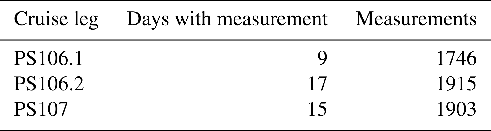
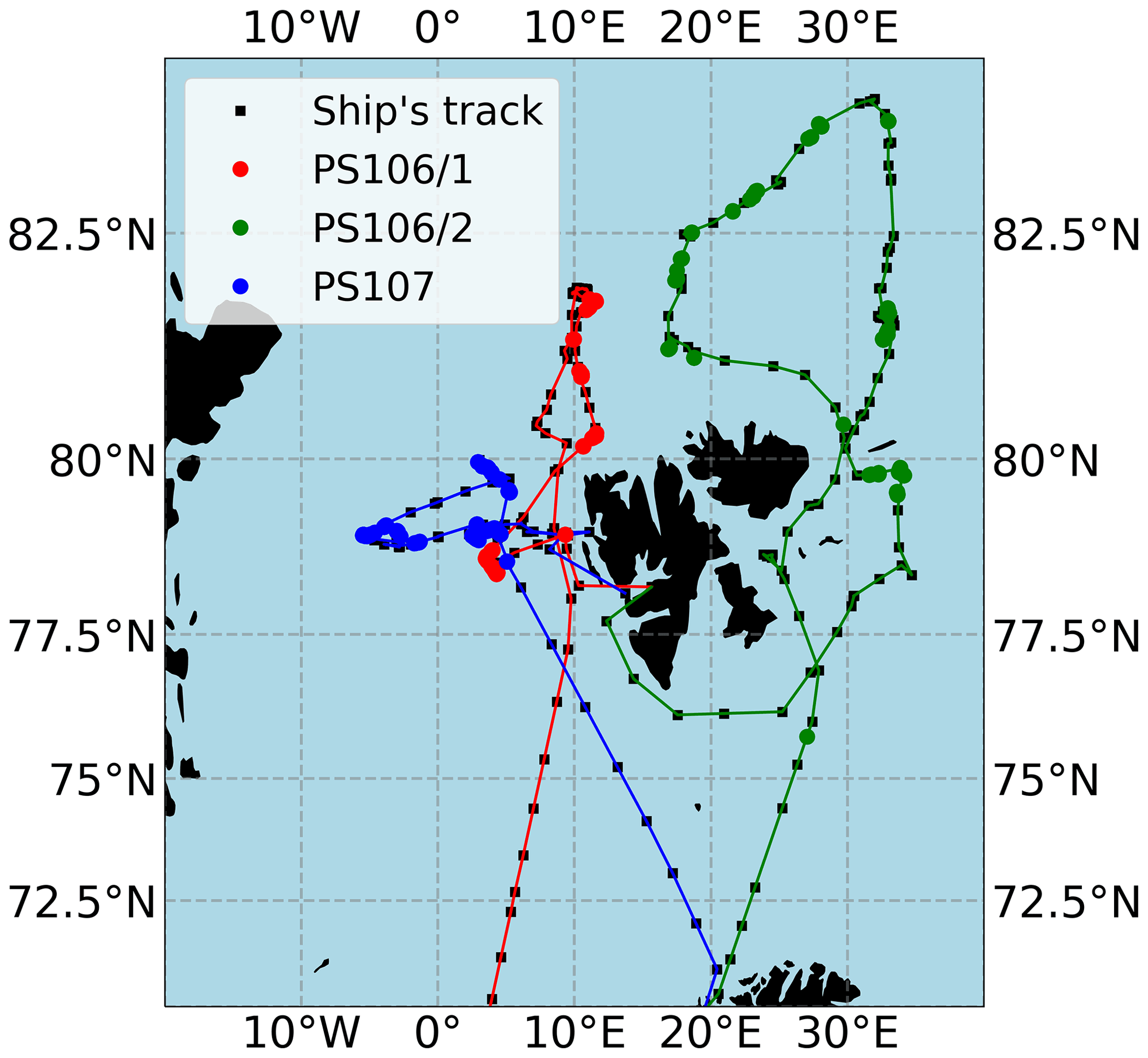
Figure 1 Map of the measurement area. Red markers indicate measurements during PS106.1 (24 May 2017 until 21 June 2017); green markers indicate measurements during PS106.2 (23 June 2017 until 19 July 2017). Blue markers indicate measurements during PS107 (22 July 2017 until 19 August 2017). The black squares show the ship's track.

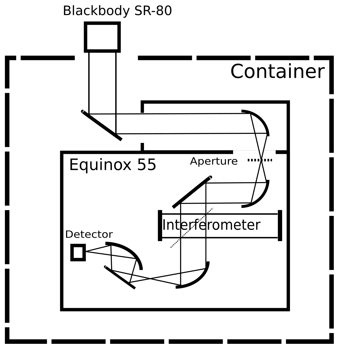
Figure 2 Sketch of IFS 55 Equinox. The blackbody SR-80 can be removed; then atmospheric radiation is measured.

2 Observations

2.1 Area of measurements

Measurements were performed around Svalbard from the 24 May 2017 until the 19 August 2017 within the scope of the cruise legs PS106.1 (PASCAL), PS106.2 (SiPCA) and PS107 (FRAM), performed by RV Polarstern. PS106.1 and PS106.2 are collectively referred to as PS106. The cloud cover was observed by meteorologists of the German Weather Service, who reported a cloud coverage of 7 or 8 oktas for approximately 75 % of the time. For further descriptions refer to Macke and Flores (2018) and Schewe (2018). Figure 1 shows the positions of the measurement sites and the ship.

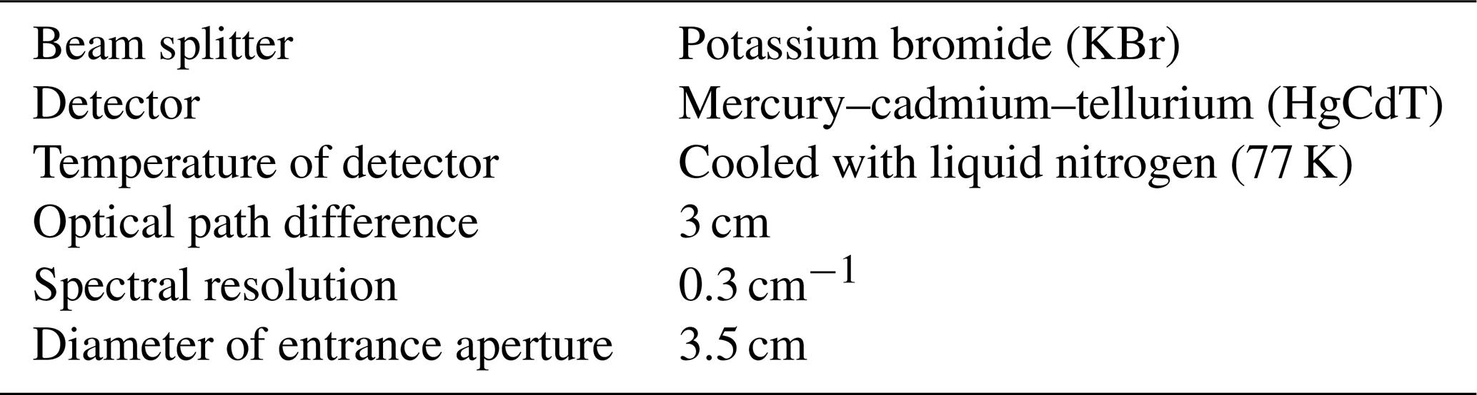
Table 2 Technical specifications of the FTIR spectrometer IFS 55 Equinox.

2.2 Measurement setup

Measurements of the atmospheric radiances are performed with a mobile FTIR spectrometer (IFS 55 Equinox by Bruker Optics GmbH) in emission mode (measures atmospheric radiation without an external light source), which will from now on be referred to as EM-FTIR. The instrument was located in an air-conditioned and insulated container on the A-Deck of RV Polarstern. The roof of the container has two openings. The EM-FTIR was located below one opening. Both openings can be closed in case of precipitation. The interferometer inside the FTIR spectrometer has a movable mirror that gives a maximum optical path difference of 3 cm, which results in a maximum spectral resolution of $\mathrm{\Delta }\overline{\mathit{\nu }}=\mathrm{0.3}{\mathrm{cm}}^{-\mathrm{1}}$. To prevent damage from the hygroscopic substance of the beam splitter (potassium bromide), the spectrometer is permanently purged with dry air. Further specifications are described in Table 2. A blackbody (SR-80 by CI Systems) is placed manually on the EM-FTIR opening at regular intervals to perform a radiometric calibration.

Figure 3 Smoothed spectral emissivity of the blackbody radiator.

2.3 Radiometric calibration and emissivity of the blackbody radiation

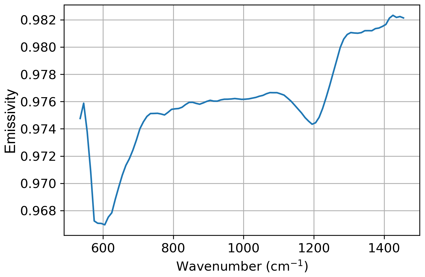
To obtain the spectral radiance L_atm, a radiometric calibration of the EM-FTIR is necessary. For this, the blackbody radiator SR-80 is used. Its temperature can be set from −10 to 125 ^∘C. The homogeneity of the radiator surface is better than ±0.05 K. The emissivity of the coating is shown in Fig. 3. The mean emissivity of the blackbody radiator is ε=0.976. An emissivity below 1 means that the radiation of the blackbody is a mixture of the Planck radiation at T_BB and the temperature of the container, which is assumed to be Planck radiation at T_lab. The radiation by the EM-FTIR is the sum of the radiation of the radiator plus a term which takes into account the temperature of the environment:

$$\begin{array}{}\text{(1)}& {\displaystyle }B=\mathit{\epsilon }B\left(T_{\mathrm{BB}}\right)+(\mathrm{1}-\mathit{\epsilon })B\left(T_{\mathrm{lab}}\right),\end{array}$$

with the temperature of the blackbody T_BB and the temperature of the laboratory T_lab weighted by the blackbody emissivity ε (Revercomb et al., 1988).

The radiometric calibration of the spectrometer is performed using

$$\begin{array}{}\text{(2)}& \begin{array}{rl}{L}_{\mathrm{atm}}& =\mathit{\epsilon }{B}_{\overline{\mathit{\nu }}}\left(T_{\mathrm{amb}}\right)+\mathit{\epsilon }{\displaystyle \frac{B_{\overline{\mathit{\nu }}}\left(T_{\mathrm{hot}}\right)-B_{\overline{\mathit{\nu }}}\left(T_{\mathrm{amb}}\right)}{\mathcal{F}(I_{\mathrm{hot}}-I_{\mathrm{amb}})}}\\ & \cdot \mathcal{F}(I_{\mathrm{atm}}-I_{\mathrm{amb}})+(\mathrm{1}-\mathit{\epsilon })B_{\overline{\mathit{\nu }}}\left(T_{\mathrm{lab}}\right).\end{array}\end{array}$$

B(T_amb), B(T_hot) and B(T_lab) are the Planck functions at high temperature (T_hot, set to 100 ^∘C), surface air temperature (T_amb) and the temperature of the laboratory (T_lab) respectively. I_hot, I_amb and I_atm are the interferograms of the hot blackbody, blackbody at ambient temperature and atmospheric measurement respectively. ℱ is the operator for the Fourier transform. In contrast to the procedure described in Revercomb et al. (1988), here the difference in the interferograms is calculated before applying the Fourier transform.

The following cycle is applied for the radiometric calibration: blackbody at T_hot, atmospheric radiation, blackbody at T_amb, atmospheric radiation, blackbody at T_hot and so on. Each measurement cycle of the blackbodies took about 10 min to obtain one blackbody interferogram I_hot or I_amb. The duration of the atmospheric measurements was approximately 15 min. The measurement time and schedule are chosen based on the time it took the blackbody to reach the desired temperature.

2.4 OCEANET measurements and Cloudnet synergistic retrieval

Retrievals of microphysical cloud parameters are compared with results of the synergistic retrieval Cloudnet. The OCEANET-Atmosphere observatory of the Leibniz Institute for Tropospheric Research (TROPOS) in Leipzig (Germany) performed continuous measurements during PS106.1 and PS106.2 (Griesche et al., 2020f). Its container houses a multi-wavelength Raman polarization lidar PollyXT and a microwave radiometer Humidity and Temperature Profiler (HATPRO), which were complemented during PS106 by a vertically pointing motion-stabilized 35 GHz cloud radar Mira-35. The OCEANET measurements provide profiles of aerosol and cloud properties and column-integrated liquid water and water vapor content. To retrieve products like liquid water content (LWC) and ice water content (IWC), the instrument synergistic approach Cloudnet (Illingworth et al., 2007) was applied to these observations. The retrieved Cloudnet dataset during PS106 has been made available via PANGAEA (see Table 7). As atmospheric input, radiosondes launched from RV Polarstern were used. If no radiosonde was available, radiosondes from Ny-Ålesund (if the ship was near Svalbard) or model data from the Global Data Assimilation System model (GDAS1) were used. A short summary of the Cloudnet retrieval is given in Appendix A. For a detailed description please refer to Griesche et al. (2020f) and the publications cited there.

3 Atmospheric profiles and cloud height information

Auxiliary data obtained in the ship cruise itself were used to construct the atmospheric setup used in the retrieval. These include temperature and humidity profiles as well as cloud ceiling measurements.

3.1 Cloud ceiling

Information about the cloud ceiling was obtained using a Vaisala CL51 ceilometer operated by the German Weather Service. The maximum cloud detection altitude is 13 km with a vertical resolution of 10 m. The uncertainty in the retrieved ceiling is ±1 % but at least ±5 m. The temporal resolution of the results is 60 s. Although only data of the cloud base height are given, it was decided to use these data instead of the Cloudnet height profile because the ceilometer data were available during the entire cruise, whereas the Cloudnet measurements were only available for PS106. Without changing the input data, a consistent dataset for the retrieval should be created. However, there is a mean bias between the cloud base height stated by Cloudnet and the ceilometer of −639 m (median bias of −47 m), which means on average the Cloudnet cloud base height is larger than the ceiling given by the ceilometer, and a root-mean-square error of 1870 m. Data of the ceilometer are available at Schmithüsen (2017a, b, c).

3.2 Radiosounding

Radiosondes were launched four times per day (00:00, 06:00, 12:00, 18:00 UTC) during PS106 and twice per day (06:00 and 12:00 UTC) during PS107 (Schmithüsen, 2017d, e, f). Data were measured using an RS92 radiosonde by Vaisala. Data of the air pressure, temperature, relative humidity, wind speed and wind direction were recorded. Accuracies are 0.5 K for temperature measurements, 5 % for relative humidity and 1 hPa for air pressure. Only atmospheric pressure, temperature and humidity were used here. Atmospheric profiles between two radiosonde launches are acquired by linear interpolation. If a radiosonde stopped measurements before reaching 30 km, data were extended using the ERA5 reanalysis (Hersbach et al., 2018).

4 Total Cloud Water retrieval (TCWret)

Total Cloud Water retrieval (TCWret) is a retrieval algorithm for microphysical cloud parameters from FTIR spectra. It is inspired by MIXCRA (Turner, 2005) and XTRA (Rathke and Fischer, 2000) and uses an optimal estimation approach (Rodgers, 2000) to invert the measured spectral radiances for retrieving microphysical cloud parameters. For a complete description of the retrieval, please refer to Appendix B.

4.1 Radiative transfer models

Two radiative transfer models are used in TCWret: the LBLRTM (Clough et al., 2005) and DISORT (Stamnes et al., 1988). DISORT is called by LBLDIS (Turner, 2005) to calculate spectral radiances.

The LBLRTM calculates the optical depth for gaseous absorbers and the water vapor continuum. Either the profiles of H₂O, CO₂, O₃, CO, CH₄ and N₂O can be set by the user, or a predefined atmosphere is used. A subarctic summer atmosphere, implemented in the LBLRTM, has been used for all gases except H₂O, which has been read from radiosonde measurements.

DISORT calculates the monochromatic radiative transfer through a vertically inhomogeneous plane-parallel medium including scattering, absorption and emission. It provides the spectral radiances using single-scatter parameters.

Several databases are included in LBLDIS (Turner, 2014). These databases contain extinction cross sections, absorption cross sections, scattering cross sections, single-scattering albedo, the asymmetry factor and phase functions for different wavenumbers and effective radii. Refractive indices for liquid water droplets and ice crystals are taken from Downing and Williams (1975) and Warren (1984) respectively. Temperature-dependent refractive indices for liquid water are from Zasetsky et al. (2005). However, it is important to note that they have large uncertainties from 1000 to 1300 cm⁻¹ (Rowe et al., 2013). Scattering properties for more complex ice particle shapes like aggregates, bullet rosettes, droxtals, hollow columns, solid columns, plates and spheroids were calculated by Yang et al. (2001) using a combination of finite-difference time domain (FDTD), geometric optics and Mie theory.

For all liquid droplets and ice crystals, the droplet size distributions follow a gamma size distribution. The gamma size distributions were chosen in a way that they fit to the data during the First International Satellite Cloud Climatology Project (ISCCP) Regional Experiment (FIRE) Arctic Cloud Experiment (ACE). For further details, please refer to Turner et al. (2003).

4.2 Products of TCWret

Direct retrieval products are τ_liq, τ_ice, r_liq and r_ice. From these parameters the water paths are calculated:

$$\begin{array}{}\text{(3)}& {\displaystyle }\text{LWP}={\displaystyle \frac{\mathrm{2}}{\mathrm{3}}}\cdot r_{\mathrm{liq}}\cdot {\mathit{\tau }}_{\mathrm{liq}}\cdot {\mathit{\varrho }}_{\mathrm{liq}},\text{(4)}& {\displaystyle }\text{IWP}={\displaystyle \frac{N\cdot V_{\mathrm{0}}\left(r_{\mathrm{ice}}\right)\cdot {\mathit{\tau }}_{\mathrm{ice}}}{{\mathit{\alpha }}_{\mathrm{ice}}}}\cdot {\mathit{\varrho }}_{\mathrm{ice}},\end{array}$$

with the volumetric mass densities of liquid water ${\mathit{\varrho }}_{\mathrm{liq}}=\mathrm{1000}\mathrm{kg}{\mathrm{m}}^{-\mathrm{3}}$ and ice water ${\mathit{\varrho }}_{\mathrm{ice}}=\mathrm{917}\mathrm{kg}{\mathrm{m}}^{-\mathrm{3}}$, the particle number density N, and the extinction coefficient ${\mathit{\alpha }}_{\mathrm{ice}}={\mathit{\beta }}_{\mathrm{ice}}\cdot N$. The total volume of an ice crystal V₀(r_ice) and the extinction cross section of an ice droplet β_ice, both integrated over the gamma size distribution, are read from the databases of single-scattering parameters. The formula for the liquid water path works for spherical droplets only, while the formula for the ice water path is valid for ice crystals of any shape (Turner, 2005). The covariance matrix S_r of the optimal estimation procedure is used to determine the errors.

4.3 Covariance matrix and averaging kernels

Retrieval errors are calculated from the variance–covariance matrix S_r of the retrieval. It is calculated by

$$\begin{array}{}\text{(5)}& {\displaystyle }{\mathbf{S}}_{\mathrm{r}}={\mathbf{T}}_{\mathrm{r}}{\mathbf{S}}_y{\mathbf{T}}_{\mathrm{r}}^T.\end{array}$$

The index r denotes quantities of the final iteration. T is a transfer matrix, and S_y is the variance–covariance matrix of the measurement. The retrieval uses a Levenberg–Marquardt algorithm; therefore the variance–covariance matrix and the transfer matrix T are calculated iteratively, as described by Ceccherini and Ridolfi (2010). Another important quantity to characterize the retrieval quality is the averaging kernel matrix A. The averaging kernel matrix contains the derivatives of the retrieved quantities with respect to the true state vector:

$$\begin{array}{}\text{(6)}& {\displaystyle }\mathbf{A}={\displaystyle \frac{\partial {\mathit{x}}_{\mathrm{r}}}{\partial {\mathit{x}}_{\mathrm{t}}}},\end{array}$$

where x_r means the retrieved parameters and x_t denotes the unknown true parameters. In TCWret, the averaging kernel matrix is a 4×4 matrix. The top two rows belong to τ_liq and τ_ice; the bottom two rows belong to r_liq and r_ice. On the diagonal elements one finds the derivatives of each element in the retrieved state vector with respect to its corresponding element in the true state vector. Off-diagonal elements give the degree of correlation between the entries of the state vector:

$$\begin{array}{}\text{(7)}& {\displaystyle }\mathbf{A}=\left(\begin{array}{cccc}{A}_{{\mathit{\tau }}_{\mathrm{liq}}}& A_{{\mathit{\tau }}_{\mathrm{liq}},{\mathit{\tau }}_{\mathrm{ice}}}& A_{{\mathit{\tau }}_{\mathrm{liq}},r_{\mathrm{liq}}}& A_{{\mathit{\tau }}_{\mathrm{liq}},r_{\mathrm{ice}}}\\ A_{{\mathit{\tau }}_{\mathrm{ice}},{\mathit{\tau }}_{\mathrm{liq}}}& A_{{\mathit{\tau }}_{\mathrm{ice}}}& A_{{\mathit{\tau }}_{\mathrm{ice}},r_{\mathrm{liq}}}& A_{{\mathit{\tau }}_{\mathrm{ice}},r_{\mathrm{ice}}}\\ A_{r_{\mathrm{liq}},{\mathit{\tau }}_{\mathrm{liq}}}& A_{r_{\mathrm{liq}},{\mathit{\tau }}_{\mathrm{ice}}}& A_{r_{\mathrm{liq}}}& A_{r_{\mathrm{liq}},r_{\mathrm{ice}}}\\ A_{r_{\mathrm{ice}},{\mathit{\tau }}_{\mathrm{liq}}}& A_{r_{\mathrm{ice}},{\mathit{\tau }}_{\mathrm{ice}}}& A_{r_{\mathrm{liq}},r_{\mathrm{ice}}}& A_{r_{\mathrm{ice}}}\end{array}\right).\end{array}$$

Here A_v,w stands for the mutual dependence of the parameters v and w, where v is the parameter in x_r and w is the parameter in x_t. The trace of the averaging kernel matrix gives the degrees of freedom of the signal, which can be interpreted as the number of individually retrievable parameters from the measurement (Rodgers, 2000). The averaging kernel matrix sets the retrieval and the a priori into context:

$$\begin{array}{}\text{(8)}& {\displaystyle }{\mathit{x}}_{\mathrm{r}}={\mathit{x}}_{\mathrm{a}}+\mathbf{A}({\mathit{x}}_{\mathrm{t}}-{\mathit{x}}_{\mathrm{a}}).\end{array}$$

From this relationship it can be seen that in the optimal case the averaging kernel matrix is the unit matrix. Smaller entries mean a stronger influence by the a priori. Averaging kernels in TCWret are calculated via

$$\begin{array}{}\text{(9)}& {\displaystyle }\mathbf{A}={\mathbf{T}}_{\mathrm{r}}{\mathbf{K}}_{\mathrm{r}}.\end{array}$$

The matrix K_r is the Jacobian matrix of the retrieved parameters (Ceccherini and Ridolfi, 2010). Uncertainties in the LWP and IWP are calculated from error propagation:

$$\begin{array}{}\text{(10)}& {\displaystyle }{\mathit{\sigma }}_Y=\pm \sqrt{\sum _i{\left({\displaystyle \frac{\partial Y}{\partial m_i}}{\mathit{\sigma }}_{m_i}\right)}^{\mathrm{2}}},\end{array}$$

where Y is either the LWP or the IWP; $\frac{\partial Y}{\partial m}$ is the partial derivative of Y with respect to an atmospheric parameter $m=\left\{{\mathit{\tau }}_{\mathrm{liq}},{\mathit{\tau }}_{\mathrm{ice}},r_{\mathrm{liq}},r_{\mathrm{ice}}\right\}$; and ${\mathit{\sigma }}_{m_i}$ is the variance of the ith parameter m_i, as stated in S_r.

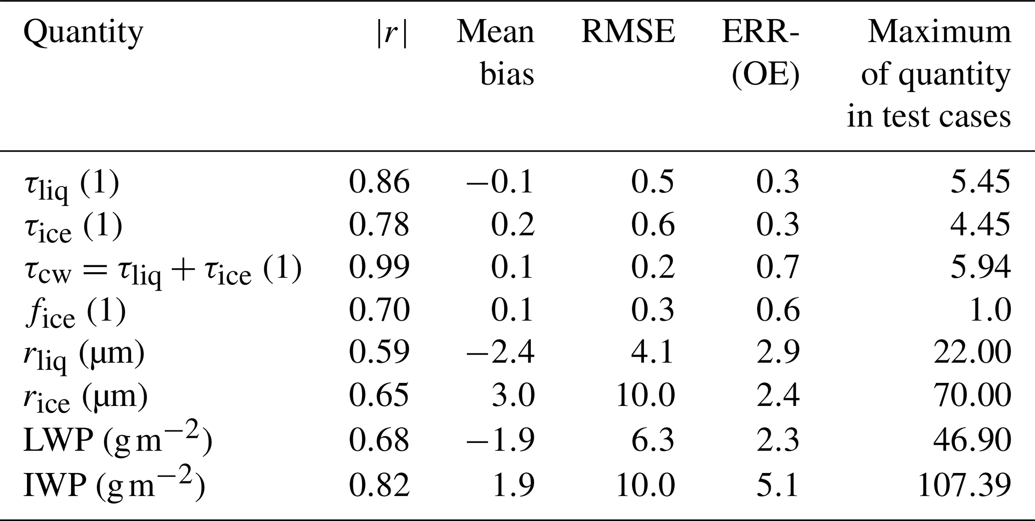
Table 3 Results of the test case retrievals. $\left|r\right|$ is the correlation coefficient of each quantity. Mean bias is the mean difference between the retrieval and the true size of the parameter. RMSE is the root-mean-square error of the difference between the retrieval and true parameter. For τ_liq,ice and r_liq,ice, ERR(OE) is the standard deviation calculated from the posterior covariance matrix of the optimal estimation, stated in Eq. (5). For the other quantities, ERR(OE) is calculated by error propagation. Maximum of quantity in test cases specifies the maximum value that can be used for this quantity in the test cases. A total number of 253 test cases are included in these calculations.

4.4 Performance of TCWret applying to simulated data

In addition to the uncertainties indicated by the optimal estimation procedure, TCWret was applied to simulated data (Cox et al., 2016). The description of the test cases and the evaluation can be found in the Appendix C. Results are shown in Table 3. When applied to the simulated data, it could be shown that TCWret can determine all variables entered in the table. Results calculated by TCWret are comparable to the true cloud parameters from the simulated data.

4.5 Errors in atmospheric profile and calibration

Besides the uncertainties from the optimal estimation algorithm, uncertainties from atmospheric profile data and the calibration cycle increase the total uncertainty in the data.

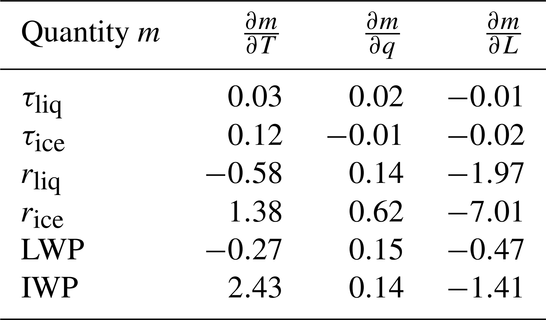
Table 4 Mean partial derivatives, used for estimating the parameter errors Δm.

Figure 4 Total error as sum of device error and interpolation error.

4.5.1 Partial derivatives for non-retrieved quantities

To estimate the uncertainty which comes from the cloud temperature, humidity profile and spectral calibration, the test cases from Cox et al. (2016) have been adjusted to incorporate uncertainties in cloud temperature, humidity and radiance. Three datasets are created, each of them with one of the following adjustments:

• increase cloud temperature by 1 K

• increase atmospheric humidity by 10 %

• increase radiance by $\mathrm{2}\mathrm{mW}({\mathrm{m}}^{\mathrm{2}}\mathrm{sr}{\mathrm{cm}}^{-\mathrm{1}}{)}^{-\mathrm{1}}$.

With these datasets the partial derivatives are calculated, which are necessary to determine the errors due to cloud temperature, humidity and spectral calibration and propagate them into the retrieved cloud parameters by application of

$$\begin{array}{}\text{(11)}& {\displaystyle }\mathrm{\Delta }m=\pm \sqrt{{\left({\displaystyle \frac{\partial m}{\partial T}}\mathrm{\Delta }T\right)}^{\mathrm{2}}+{\left({\displaystyle \frac{\partial m}{\partial q}}\mathrm{\Delta }q\right)}^{\mathrm{2}}+{\left({\displaystyle \frac{\partial m}{\partial L}}\mathrm{\Delta }L\right)}^{\mathrm{2}}},\end{array}$$

with the cloud temperature T; the relative humidity q; the radiance L; and their errors ΔT, Δq and ΔL. To separate the influence of the parameter errors from the retrieval performance, the results of these three datasets are compared to the retrieval results mentioned in Sect. 4.4 instead of the true cloud parameters. Mean partial derivatives are then calculated as follows:

1. Retrieve the cloud parameters for each dataset.

2. Calculate the difference between the cloud parameters of the adjusted dataset and the undisturbed dataset (which has been already used in Sect. 4.3).

3. Calculate the difference quotients, which will act as partial derivatives in Eq. (11).

The partial derivatives are shown in Table 4.

4.5.2 Temperature and humidity

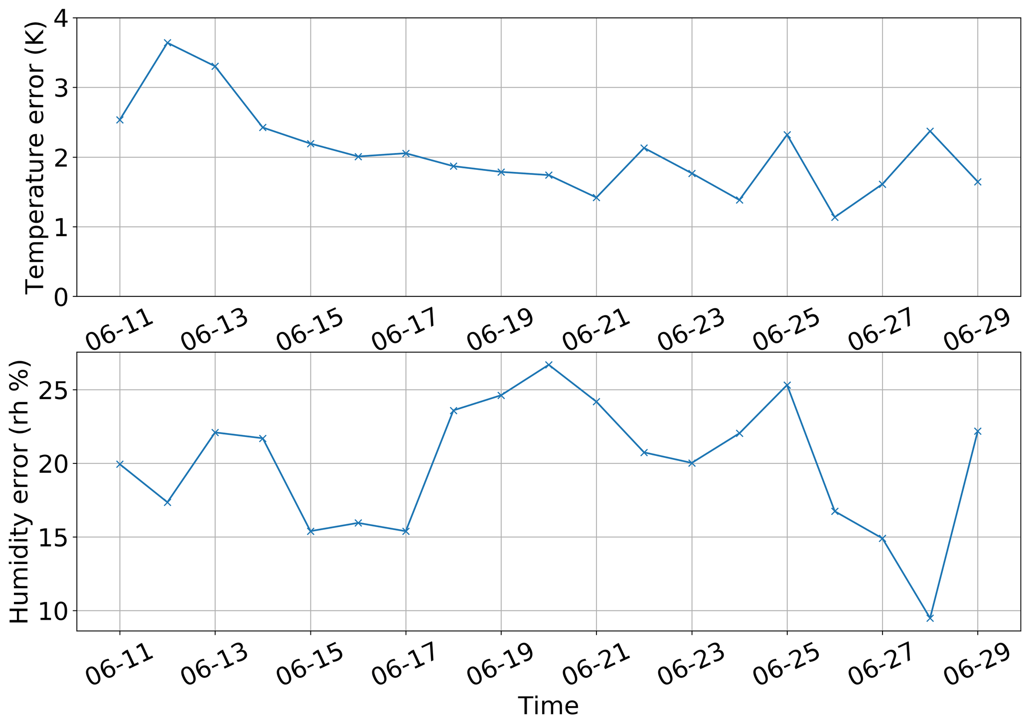
Device errors in the radiosonde are ΔT=0.5 K and Δq=5 %. Additionally, the error introduced with the linear interpolation of the temperature and relative humidity is estimated by comparing the interpolated profiles to atmospheric profiles from ERA5. The interpolation error follows from the comparison between the linear interpolation between two radiosonde measurements and the ERA5 atmosphere at the position of the measurements. We query the ERA5 atmosphere for each hour. Then we calculate the atmospheric profiles from the radiosondes once per hour by linear interpolation. From this we calculate the difference, average over 1 d and calculate the standard deviation. Figure 4 gives the total error as device error and interpolation error, as an example for the period from 11 June 2017 to 30 June 2017.

4.5.3 Calibration error

The accuracy of the blackbody temperature and emissivity are $\mathrm{\Delta }{T}_{\mathrm{BB}}=\pm \mathrm{0.05}\mathrm{K}$ and $\mathrm{\Delta }\mathit{ϵ}=\pm \mathrm{0.02}$. The propagation of these errors into the radiance is

$$\begin{array}{}\text{(12)}& {\displaystyle }\mathrm{\Delta }L=\sqrt{{\left({\displaystyle \frac{\partial L_{\mathrm{atm}}}{\partial \mathit{ϵ}}}\cdot \mathrm{0.02}\right)}^{\mathrm{2}}+{\left({\displaystyle \frac{\partial L_{\mathrm{atm}}}{\partial T_{\mathrm{BB}}}}\cdot \mathrm{0.05}\mathrm{K}\right)}^{\mathrm{2}}}.\end{array}$$

To estimate $\frac{\partial L_{\mathrm{atm}}}{\partial \mathit{ϵ}}$, a spectrum is calibrated with an emissivity of ϵ^′ and ${\mathit{ϵ}}^{\prime }+h$. The partial derivative is calculated by $\frac{\partial L_{\mathrm{atm}}}{\partial \mathit{ϵ}}=\frac{L({\mathit{\epsilon }}^{\prime }+h)-L\left({\mathit{\epsilon }}^{\prime }\right)}{h}$ with L(ε^′) being the radiance under the emissivity ε^′ and h as the step size for the numerical calculation of the partial derivative. From ${\mathit{ϵ}}^{\prime }=\mathrm{0.975}$ and h=0.02 follows $\frac{\partial L_{\mathrm{atm}}}{\partial \mathit{ϵ}}\cdot \mathrm{0.02}=-\mathrm{0.98}\mathrm{mW}({\mathrm{m}}^{\mathrm{2}}\mathrm{sr}{\mathrm{cm}}^{-\mathrm{1}}{)}^{-\mathrm{1}}$. The second partial derivative $\frac{\partial L_{\mathrm{atm}}}{\partial T_{\mathrm{BB}}}$ is estimated using Eq. (2). The emissivity is set to 1. The measured radiance of the hot blackbody is larger than the radiance of the atmosphere (ℱ(I_hot)>ℱ(I_atm)), and therefore the quotient

$$\begin{array}{}\text{(13)}& {\displaystyle \frac{\mathcal{F}(I_{\mathrm{atm}}-I_{\mathrm{amb}})}{\mathcal{F}(I_{\mathrm{hot}}-I_{\mathrm{amb}})}}<\mathrm{1}.\end{array}$$

From the measurements it follows that L_hot is about 5 times larger than L_amb; therefore the inequation (Eq. 13) is set as $\frac{\mathcal{F}(I_{\mathrm{hat}}-I_{\mathrm{amb}})}{\mathcal{F}(I_{\mathrm{hot}}-I_{\mathrm{amb}})}=\mathrm{0.2}$. Equation (2) thus can be written as

$$\begin{array}{}\text{(14)}& {\displaystyle }{L}_{\mathrm{atm}}=B_{\overline{\mathit{\nu }}}\left(T_{\mathrm{amb}}\right)+\mathrm{0.2}\cdot B_{\overline{\mathit{\nu }}}\left(T_{\mathrm{hot}}\right)-B_{\overline{\mathit{\nu }}}\left(T_{\mathrm{amb}}\right).\end{array}$$

With $T_{\mathrm{BB}}=T_{\mathrm{hot}}=\mathrm{100}$ ^∘C and T_amb=0 ^∘C, $\frac{\partial L_{\mathrm{atm}}}{\partial T_{\mathrm{BB}}}\cdot \mathrm{0.05}=\mathrm{0.10}\mathrm{mW}({\mathrm{m}}^{\mathrm{2}}\mathrm{sr}{\mathrm{cm}}^{-\mathrm{1}}{)}^{-\mathrm{1}}$ is an average for the spectral interval between 500 and 2000 cm⁻¹. This gives $\mathrm{\Delta }L=\mathrm{0.98}\mathrm{mW}({\mathrm{m}}^{\mathrm{2}}\mathrm{sr}{\mathrm{cm}}^{-\mathrm{1}}{)}^{-\mathrm{1}}$.

4.5.4 Resulting parameter error

Finally, from the calculations in this section, the resulting uncertainties are as follows:

• ΔT=2.0 K, as the sum of the device error (0.5 K) and the interpolation error (1.5 K).

• Δq=17.5 %, as the sum of the device error (5.0 %) and the interpolation error (12.5 %).

• $\mathrm{\Delta }L=\mathrm{0.98}\mathrm{mW}({\mathrm{m}}^{\mathrm{2}}\mathrm{sr}{\mathrm{cm}}^{-\mathrm{1}}{)}^{-\mathrm{1}}$.

Applying these uncertainties to Eq. (11), the uncertainties for each parameter are Δτ_liq=0.4, Δτ_ice=0.3, Δr_liq=3.3 µm, Δr_ice=13.1 µm, $\mathrm{\Delta }\text{LWP}=\mathrm{2.8}\mathrm{g}{\mathrm{m}}^{-\mathrm{2}}$ and $\mathrm{\Delta }\text{IWP}=\mathrm{5.6}\mathrm{g}{\mathrm{m}}^{-\mathrm{2}}$. These values will be added to the retrieval errors in the next section.

Figure 5 Distribution of retrieved optical depths for liquid water (a) and ice water (b). The bin width is set to the sum of the root-mean-square error from Table 3 and the errors discussed in Sect. 4.5.

Figure 6 Distribution of the retrieved LWP (a) and IWP (b). The bin width is set to the sum of the root-mean-square error from Table 3 and the errors discussed in Sect. 4.5.

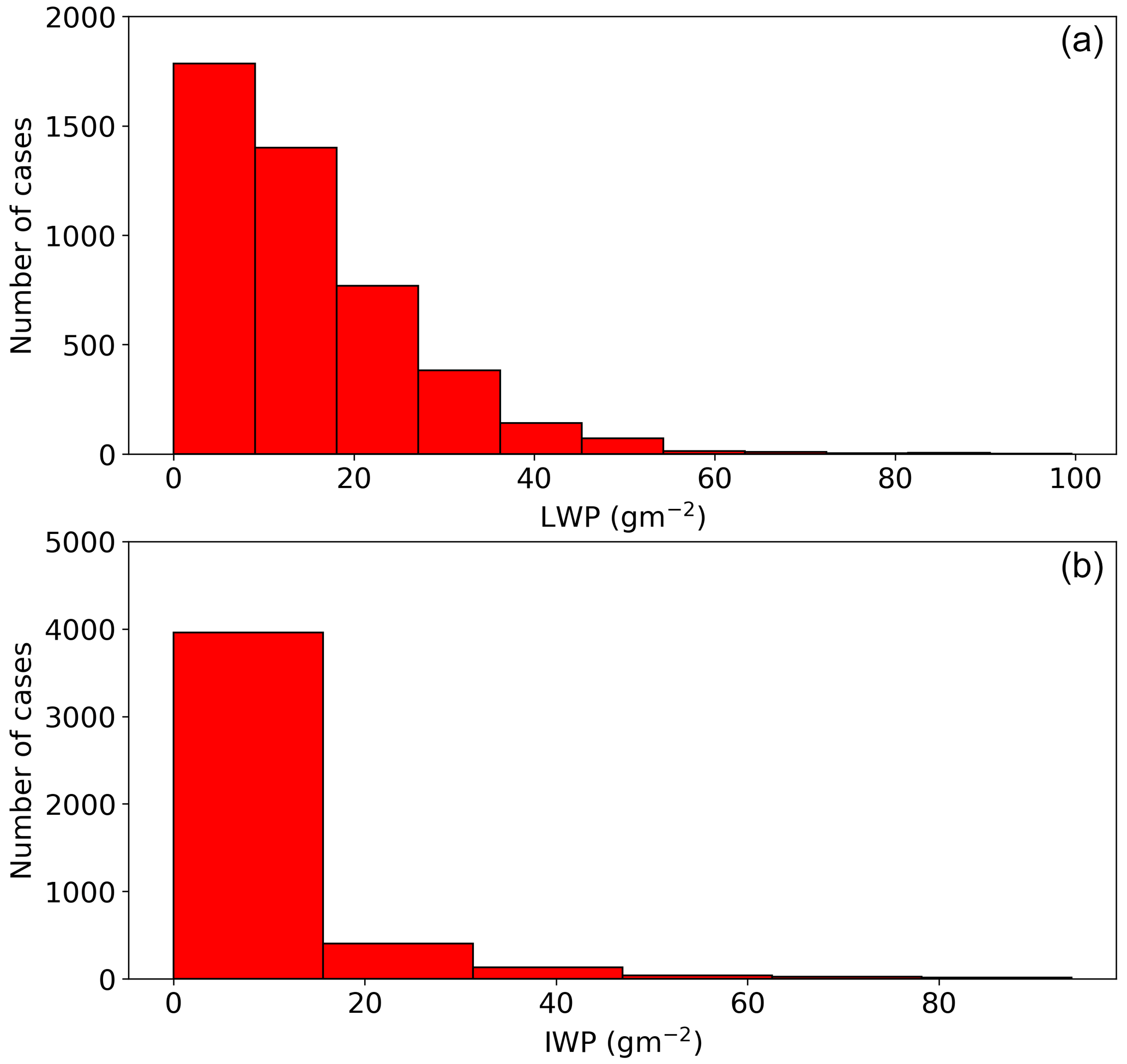
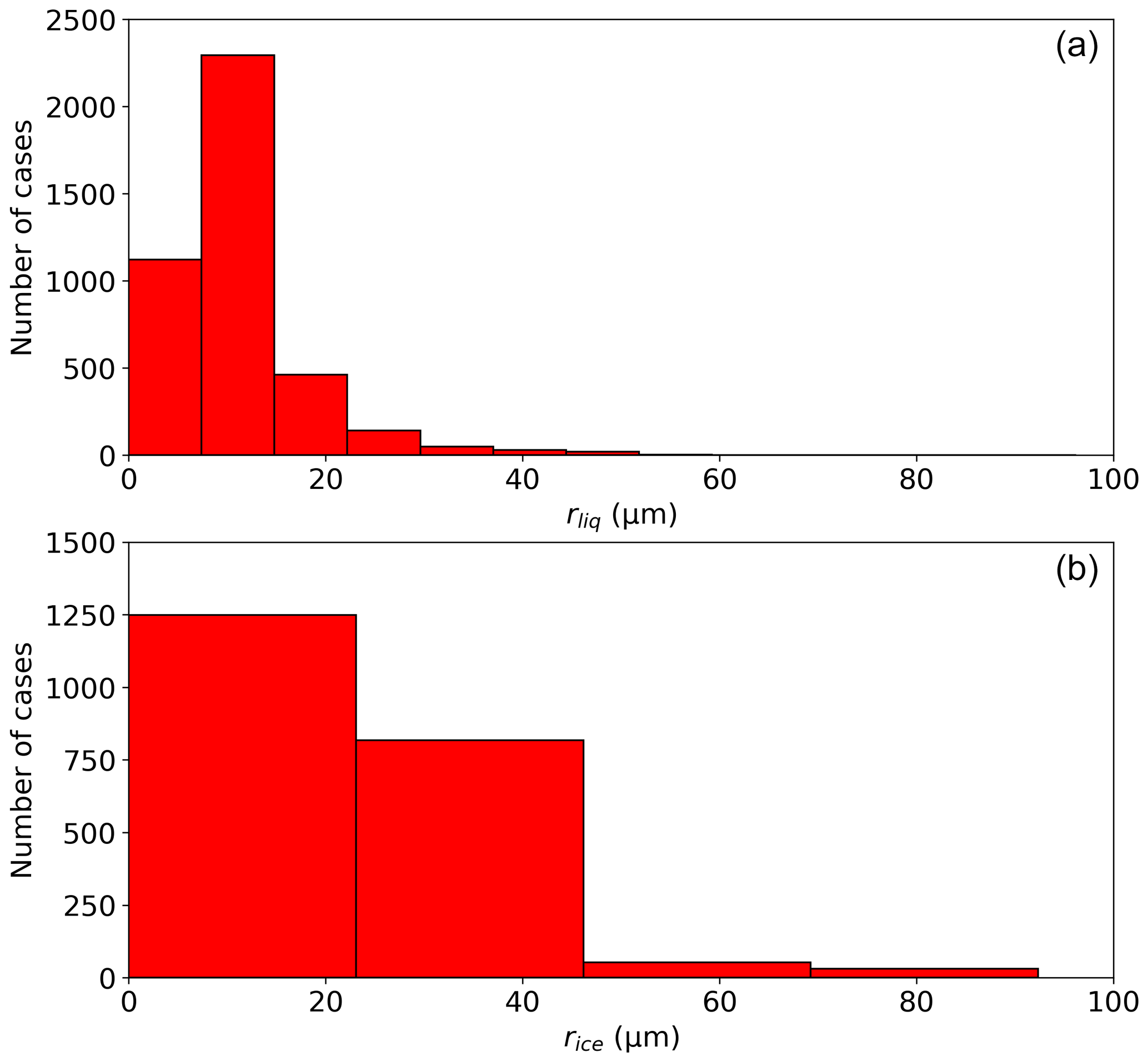
Figure 7 Distribution of retrieved effective radii for liquid water droplets (a) and ice crystals (b). The bin width is set to the sum of the root-mean-square error from Table 3 and the errors discussed in Sect. 4.5. In each instance, only cases are considered in which the phase fractions are above 0.1 (liquid water fraction for r_liq and ice water fraction for r_ice). This results in 4111 of 4590 cases for r_liq (89.6 %) and 2153 of 4590 cases for r_ice (46.9 %).

Table 5 Key features of the dataset.

5 Results

5.1 Cloud parameters from infrared radiance measurements during PS106 and PS107

During the measurement campaign, most of the observed optical depth is due to liquid water instead of ice crystals. Histograms of all retrieved optical depths are shown in Fig. 5. In 66.4 % of the measurements, ice was observed in the clouds, whereas in 92.4 % of the measurements liquid water was present. Mean optical depths are τ_liq=2.6 and τ_ice=0.8. Similarly to the optical depth, most of the observed cloud water is liquid water (Fig. 6). Here the means are $\text{LWP}=\mathrm{17.7}\mathrm{g}{\mathrm{m}}^{-\mathrm{2}}$ and $\text{IWP}=\mathrm{9.9}\mathrm{g}{\mathrm{m}}^{-\mathrm{2}}$. Interquartile ranges for the LWP and IWP are ${\mathrm{IQR}}_{\mathrm{LWP}}=\mathrm{18.9}\mathrm{g}{\mathrm{m}}^{-\mathrm{2}}$ and ${\mathrm{IQR}}_{\mathrm{IWP}}=\mathrm{11.5}\mathrm{g}{\mathrm{m}}^{-\mathrm{2}}$. Whereas the range of the LWP matches the LWP from the test cases, the IWP is near the lower threshold of the retrievable water path.

The distributions of the effective radii are shown in Fig. 7. For r_liq only cases with f_ice<0.9 are used, and for r_ice only cases with f_ice>0.1 are used. On average, ice crystals (r_ice=22.3 µm) are larger than liquid droplets (r_liq=10.9 µm). Ice crystals show a wider range of retrieved effective radii than liquid droplets, expressed by an interquartile range of IQR_ice=17.9 µm compared to IQR_liq=5.9 µm.

5.2 Averaging kernels and posterior correlation matrices

For all measurements, the mean of the averaging kernels and degrees of freedom are calculated:

$$\begin{array}{}\text{(15)}& {\displaystyle }\mathbf{A}& {\displaystyle }=\left(\begin{array}{cccc}\mathrm{0.77}& \mathrm{0.48}& -\mathrm{0.17}& -\mathrm{0.02}\\ \mathrm{0.19}& \mathrm{0.45}& \mathrm{0.25}& -\mathrm{0.01}\\ -\mathrm{0.04}& \mathrm{0.14}& \mathrm{0.74}& \mathrm{0.05}\\ -\mathrm{0.03}& -\mathrm{0.1}& \mathrm{0.29}& \mathrm{0.3}\end{array}\right),\text{(16)}& {\displaystyle }tr\left(\mathbf{A}\right)& {\displaystyle }=\mathrm{2.25}.\end{array}$$

This mean averaging kernel matrix contains both single-phase clouds and mixed-phase clouds. Since only two parameters are determined in the single-phase cases, they perturb the mean number of degrees of freedom for all measurements. As seen in the statistics, there are fewer cases with ice-containing clouds. This lowers the entries on the diagonals for τ_ice and r_ice as they are 0 in all-liquid clouds. Therefore, the mean averaging kernel was also calculated for all mixed-phase clouds:

$$\begin{array}{}\text{(17)}& {\displaystyle }{\mathbf{A}}_{\text{mixed-phase}}=\left(\begin{array}{cccc}\mathrm{0.62}& \mathrm{0.22}& -\mathrm{0.35}& -\mathrm{0.03}\\ \mathrm{0.32}& \mathrm{0.7}& \mathrm{0.47}& -\mathrm{0.04}\\ -\mathrm{0.08}& \mathrm{0.16}& \mathrm{0.66}& \mathrm{0.1}\\ -\mathrm{0.14}& -\mathrm{0.07}& \mathrm{0.17}& \mathrm{0.59}\end{array}\right)\text{(18)}& {\displaystyle }tr\left({\mathbf{A}}_{\text{mixed-phase}}\right)=\mathrm{2.57}\end{array}$$

The number of degrees of freedom in this case is 2.57. The entries for the effective radii are of the same size as those for the optical depth.

The posterior correlation matrix R gives the correlations of one retrieved parameter to another. For mixed-phase clouds, R is as follows:

$$\begin{array}{}\text{(19)}& {\displaystyle }{\mathbf{R}}_{\text{mixed-phase}}{\displaystyle }=\left(\begin{array}{cccc}\mathrm{1.00}& \mathrm{0.50}& -\mathrm{0.07}& -\mathrm{0.40}\\ \mathrm{0.50}& \mathrm{1.00}& \mathrm{0.02}& -\mathrm{0.23}\\ -\mathrm{0.07}& \mathrm{0.02}& \mathrm{1.00}& \mathrm{0.13}\\ -\mathrm{0.41}& -\mathrm{0.23}& \mathrm{0.13}& \mathrm{1.00}\end{array}\right).\end{array}$$

The largest correlation appears between τ_liq and τ_ice ($\left|r\right|=\mathrm{0.50}$), which points to a difficult phase determination. Apart from the correlation of the optical depths, the comparatively high correlation between r_ice and τ_liq is striking, which suggests that both parameters cannot be determined completely independently of each other.

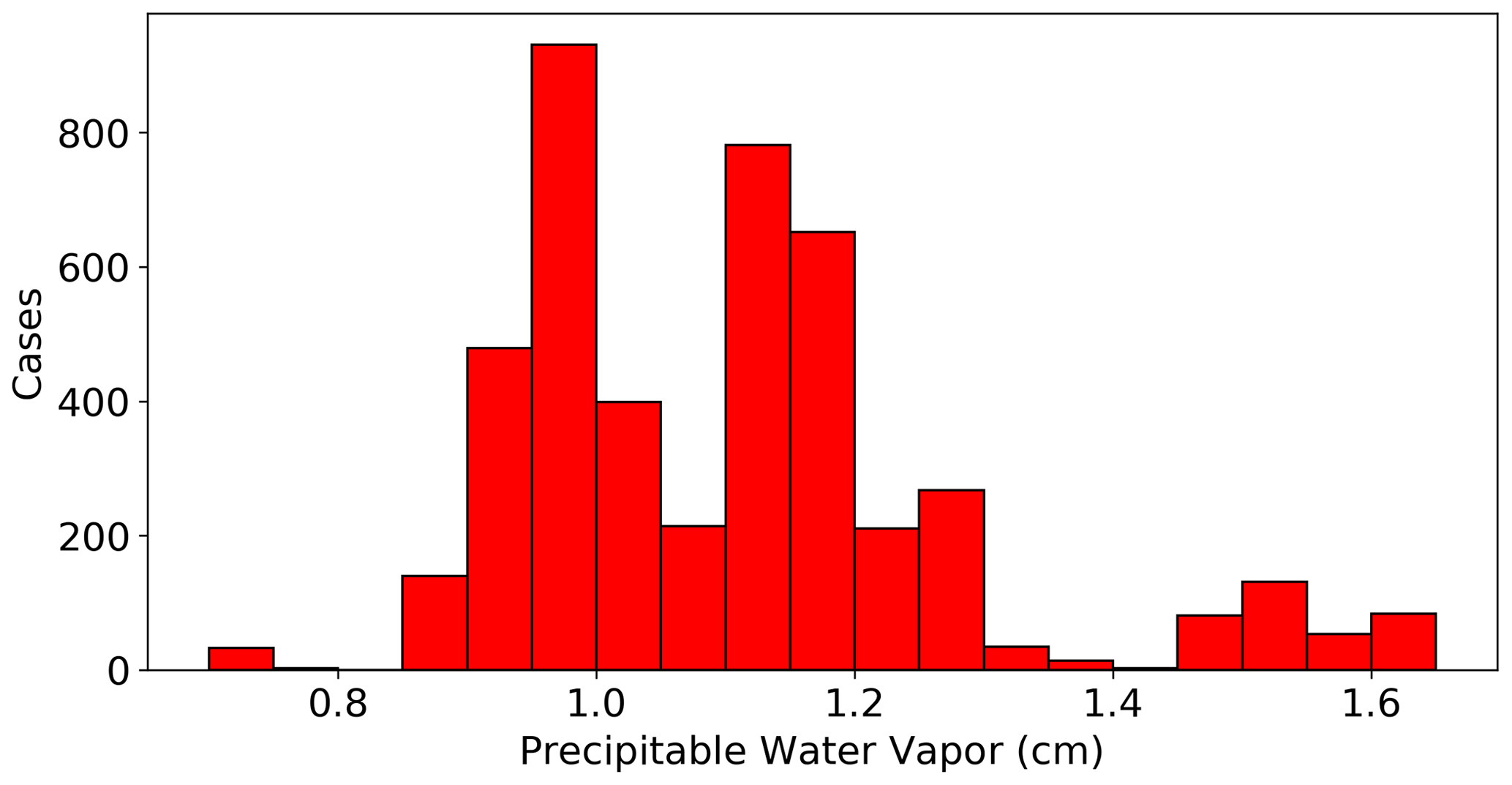
Figure 8 Histogram of the precipitable water vapor during the measurements of atmospheric radiances.

Figure 9 Percentage of retrievals for each ice particle shape. Most particles are modeled as droxtals (37 %), solid columns (35 %), plates (22 %) and bullet rosettes (4 %).

5.3 Precipitable water vapor

A crucial spectral region for the determination of the cloud phase is the spectral window in the far infrared between 500 and 600 cm⁻¹ (Rathke et al., 2002). This spectral region is sensitive to the concentration of water vapor in the atmosphere. The amount of water vapor is expressed by the precipitable water vapor PWV, which has been calculated from the radiosonde measurements. The far-infrared spectral region becomes nearly opaque to infrared radiation for PWV >1 cm (Cox et al., 2015). During the measurement campaign the PWV was greater than 1 cm in 62 % of the cases. Therefore, the datasets for PWV greater than 1 cm are not removed from the analysis. Statistics of PWV are shown in Fig. 8.

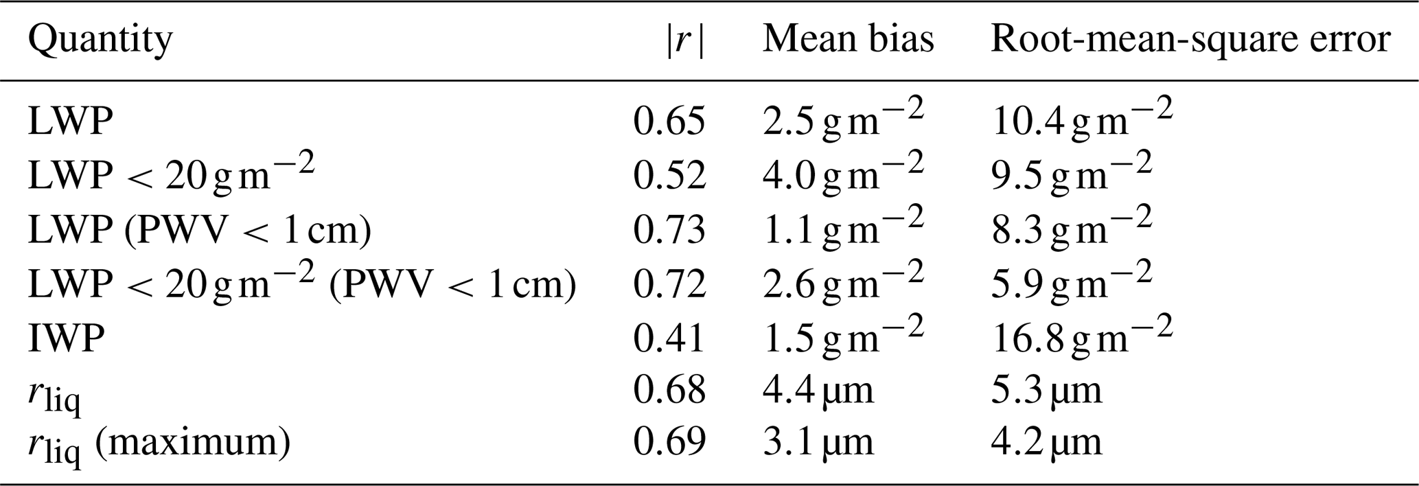
Table 6 Results of the comparison between TCWret and Cloudnet. Mean bias and root-mean-square error refer to the difference in both datasets.

5.4 Comparison to Cloudnet

To compare results from TCWret and Cloudnet, a combined dataset of TCWret results is created in the following way. Since the shapes of the ice crystals are not known, the retrievals were carried out for all ice crystal shapes. However, this procedure leads to up to eight results per measurement, so a selection was made. The aim of the following selection is that all ice crystals with r_ice<30 µm are modeled as droxtals, while larger ice crystals are modeled as plates, bullet rosettes or solid columns. This choice is motivated by Yang et al. (2007). The accepted result is then determined as follows:

1. If r_ice for plates, bullet rosettes and solid columns or for droxtals is less than 30 µm, the result using ice crystals as droxtals is accepted.

2. If r_ice for droxtals is greater than 10 µm, the result that uses plates, bullet rosettes or solid columns is accepted. To choose one of the datasets, a random number is drawn which selects plates in 35 %, bullet rosettes in 15 % and solid columns in 50 % of cases.

3. If none of the conditions apply, the data for which the degrees of freedom of the outcome are highest are accepted.

The first condition ensures that all small ice particles are classified as droxtals, while the second ensures that all larger particles are classified as plates, solid columns or bullet rosettes. Stricter thresholds would more often result in only the last condition applying, which should be avoided as much as possible.

As an additional constraint, we only allow results where r_liq<r_ice. This is motivated by the following: the results of r_liq and r_ice show that r_liq is usually smaller than r_ice. This applies to both TCWret and Cloudnet. Therefore, cases with r_liq>r_ice are likely cases with a too small r_ice and a too large r_liq. For the comparison between TCWret and Cloudnet, results from both datasets were averaged over a time period of 2 min. This has been done because the underlying measurement systems have different temporal resolutions; also both measurement systems were at different locations on the ship. Cloudnet results do not contain optical depths but water paths and droplet radii; therefore we will compare the LWP and IWP, r_liq and r_ice. Correlation coefficients, mean biases and root-mean-square errors are shown in Table 6.

Figure 10 The IWP of TCWret versus the IWP from Cloudnet.

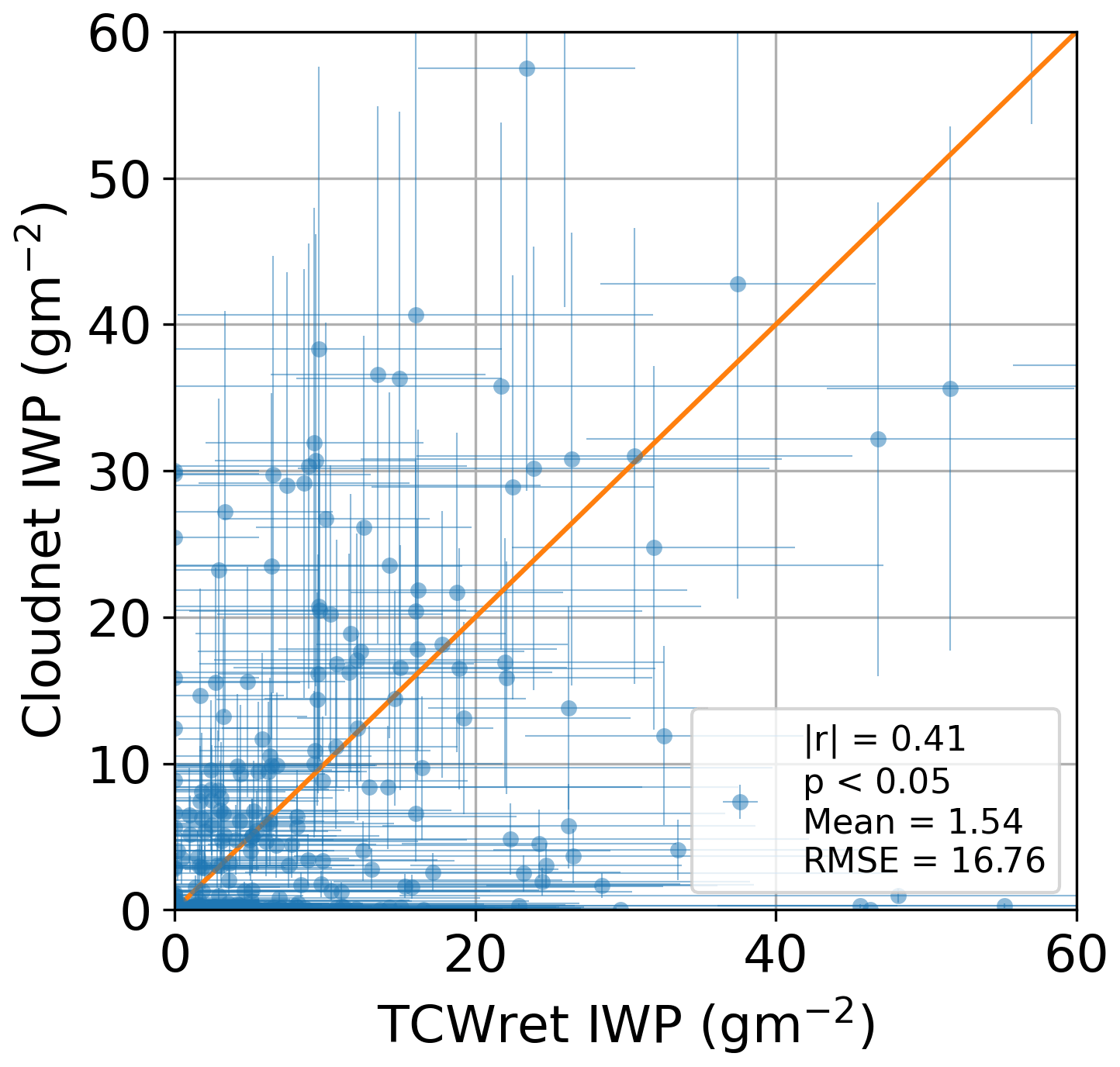
5.4.1 Ice water path and ice effective radius

Although TCWret can determine r_ice from the simulated spectra, no correlation can be found between the TCWret and Cloudnet data. From the error considerations in previous sections it was shown that the RMSE for the simulated spectra is already 10.0 µm. Taking into account uncertainties in the atmospheric data and the calibration, an additional uncertainty term of 13.1 µm is obtained, so r_ice is already subject to high uncertainties. According to the posterior correlation matrix, r_ice correlates with τ_liq, so there is no completely independent result of r_ice. A better determination of r_ice could be achieved by a better a priori x_a, but the problem remains that according to the averaging kernel matrix, only 2.57 degrees of freedom exist in the measurements.

Figure 10 shows the results for the IWP. Although a correlation can be found, there is large spread between the datasets. The difference between TCWret and Cloudnet is $(\mathrm{1.5}\pm \mathrm{16.8})\mathrm{g}{\mathrm{m}}^{-\mathrm{2}}$. The IWP is calculated according to Eq. (4) from τ_ice and r_ice, where r_ice influences the IWP of the TCWret dataset. Furthermore, the IWP during the measurement campaign is 9.9 g m⁻², very low and within the RMSE of TCWret when retrieving the simulated spectra. The IWP is therefore at the lower limit of what can be determined with TCWret and is considered less reliable.

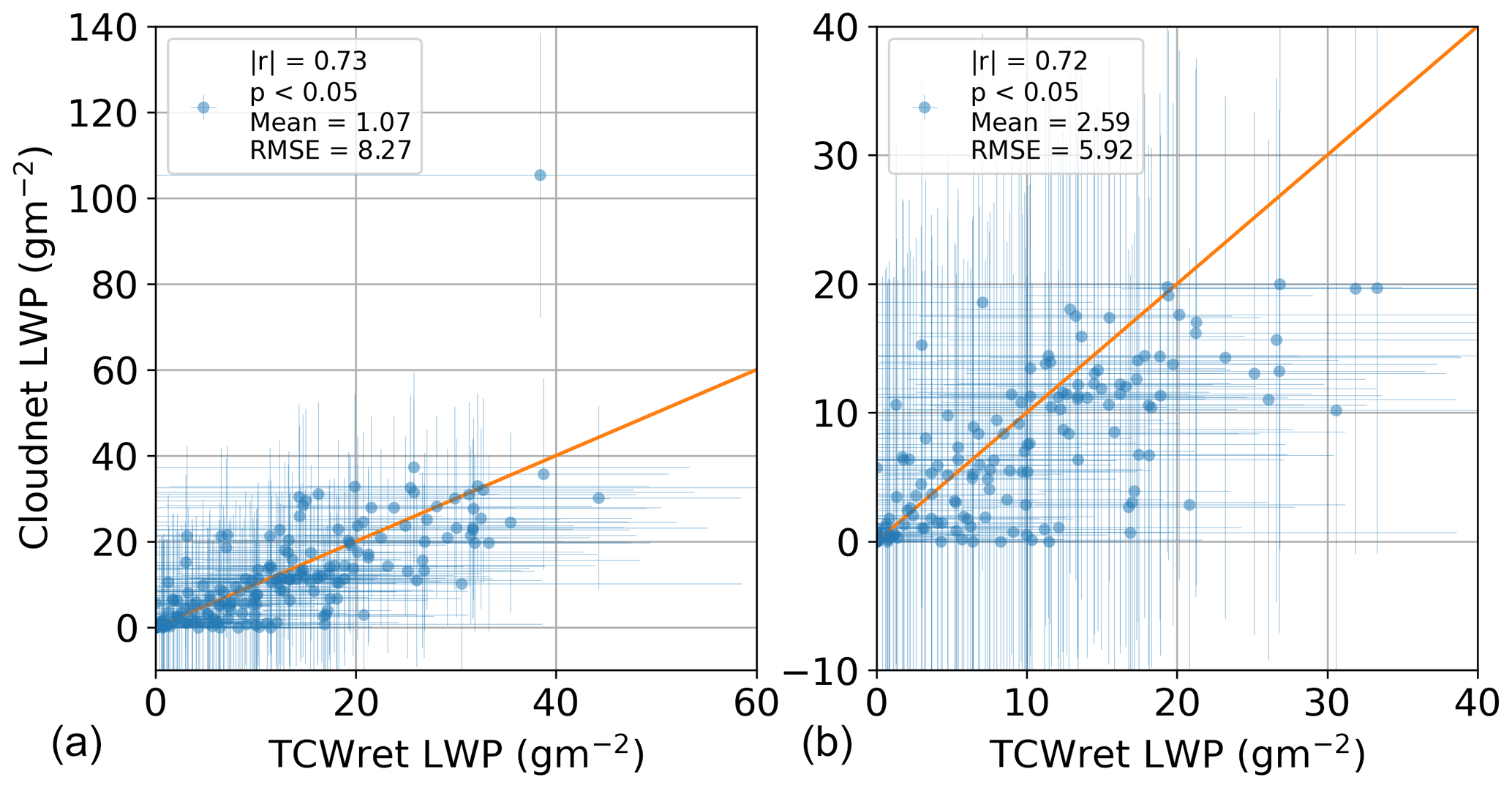
Figure 11 Liquid water path of TCWret versus Cloudnet for PWV<1 cm. Left scatterplot (a) contains all measurements, whereas the right plot (b) only shows clouds with LWP $<\mathrm{20}\mathrm{g}{\mathrm{m}}^{-\mathrm{2}}$.

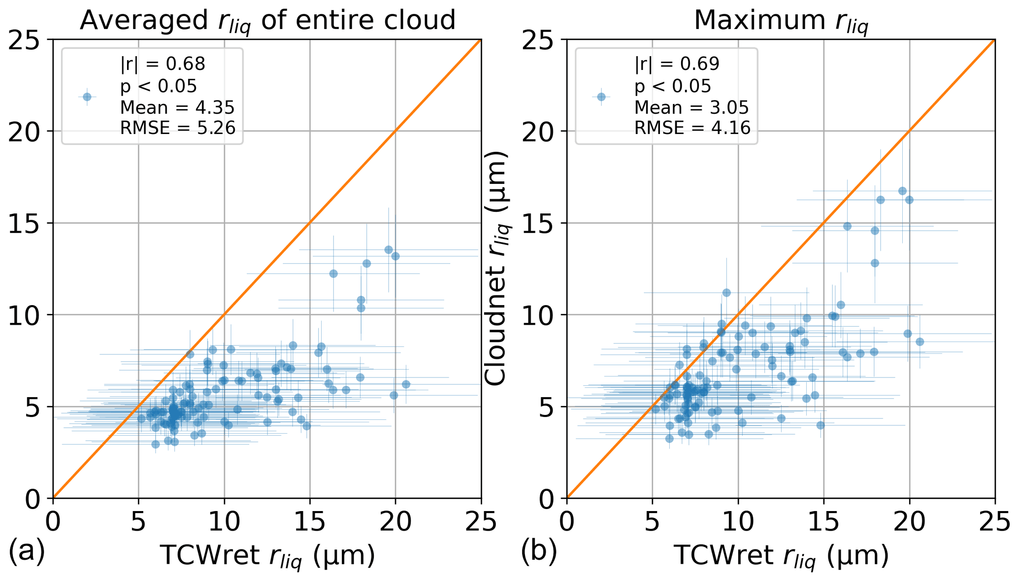
Figure 12 The r_liq of TCWret versus r_liq of Cloudnet averaged over the entire cloud (a) and maximum value of the cloud from Cloudnet (b).

5.4.2 Liquid water path and effective droplet radius

Results of the liquid water path from TCWret and Cloudnet are correlated. The difference is ($\mathrm{2.5}\pm \mathrm{10.4})\mathrm{g}{\mathrm{m}}^{-\mathrm{2}}$ with no restriction to the maximum water path. From this we conclude that the LWP from the TCWret dataset is reliable. As mentioned earlier, a large PWV value interferes with the retrieval, as the water vapor has a larger influence on the microwindows. Therefore, we additionally remove all cases from the analysis where the PWV is larger than 1 cm. This reduces the mean bias to 1.1 g m⁻² and the RMSE to 8.3 g m⁻². The results with PWV <1 cm are shown in Fig. 11, left panel.

Since the LWP of TCWret correlates with that of the Cloudnet product and since the RMSE of the LWP is far below the uncertainty in the LWP of the Cloudnet product, we reduced the maximum LWP to investigate whether a correlation can also be observed for clouds with an $\text{LWP}<\mathrm{20}\mathrm{g}{\mathrm{m}}^{-\mathrm{2}}$. With a real uncertainty of $\pm \mathrm{20}\mathrm{g}{\mathrm{m}}^{-\mathrm{2}}$ the correlation is expected to disappear.

Results for very thin clouds and PWV <1 cm are shown in Fig. 11 (right side). Again, results are correlated. The RMSE for these clouds is 5.9 g m⁻² with a mean bias of 2.6 g m⁻². Without any restrictions on the PWV, there is an RMSE of 9.5 g m⁻² and a mean bias of 4.0 g m⁻². From the comparison with TCWret, it can be concluded that during this measurement campaign, Cloudnet's results for thin clouds with LWP $<\mathrm{20}\mathrm{g}{\mathrm{m}}^{-\mathrm{2}}$ are also reliable despite the stated error of 20.40 g m⁻².

It should be noted that Cloudnet and TCWret use the atmospheric profiles from the radiosonde measurements carried out on RV Polarstern. Apart from that, however, both the measuring instruments and the retrievals are different. Furthermore, TCWret does not use information from Cloudnet as a priori. Since TCWret has also shown comparable agreement with the LWP of the simulated spectra in the test cases (mean bias is $-\mathrm{1.6}\mathrm{g}{\mathrm{m}}^{-\mathrm{2}}$; RMSE is 6.3 g m⁻²), it is to be expected that TCWret and thus also Cloudnet have independently determined the LWP correctly.

Figure 12 shows the results for r_liq. The left panel shows the results where r_liq of Cloudnet is averaged over the entire cloud. The right panel shows the maximum r_liq of the cloud in the Cloudnet data. Only results from TCWret are considered if f_ice<0.9. As in the LWP, a correlation between the data can be observed. Overall, there is an overestimation of the r_liq of TCWret by 4.4 µm on average. If only considering the maximum r_liq in Cloudnet, the mean bias decreases to 3.1 µm. The same applies to the RMSE, which decreases from 5.3 to 4.2 µm. These results indicate that r_liq in TCWret does not take into account the entire cloud, which is to be expected since the r_liq in Cloudnet is determined using the altitude-resolved radar reflectivity, while TCWret uses the radiance of the clouds measured on the ground. However, the observed correlation allows a correction of r_liq in TCWret as a function of r_liq itself.

Richter et al. (2021)Griesche et al. (2020a)Griesche et al. (2020b)Griesche et al. (2020c)Griesche et al. (2020d)Griesche et al. (2020e)Schmithüsen (2017a)Schmithüsen (2017b)Schmithüsen (2017c)Schmithüsen (2017d)Schmithüsen (2017e)Schmithüsen (2017f)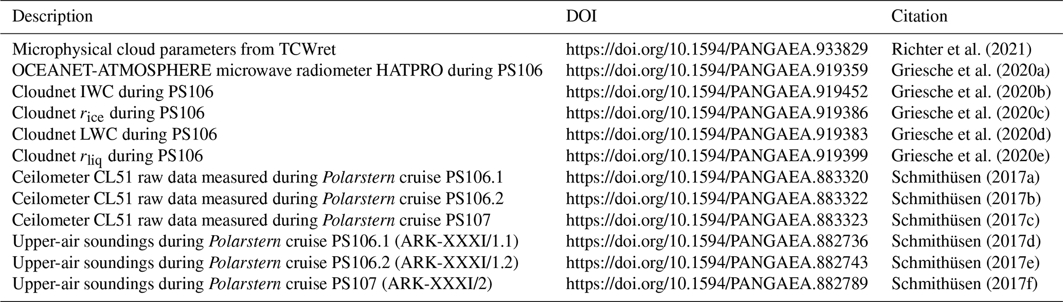

Table 7 Datasets used in this publication.

6 Code availability

The retrieval algorithm TCWret is available at https://doi.org/10.5281/ZENODO.4621127 (Richter, 2021a) with external subroutines at https://doi.org/10.5281/ZENODO.4618142 (Richter, 2021b) and https://doi.org/10.5281/ZENODO.4618106 (Richter, 2021c). Jupyter notebooks to perform the comparisons to Cloudnet are available at https://doi.org/10.5281/zenodo.6647314 (Richter, 2022).

7 Data availability

For accessibility of the datasets used and shown, see Table 7.

8 Summary and conclusion

A dataset of microphysical cloud parameters of optically thin clouds is presented. The measurements were carried out on the ship RV Polarstern in summer 2017 in the Arctic Ocean around Svalbard and in the Fram Strait.

Measurements were performed using a mobile FTIR spectrometer, operated in emission mode (EM-FTIR). A calibration of the EM-FTIR was performed with a blackbody radiator, whose temperature was alternately set to 100 ^∘C and ambient temperature. The spectrometer was operated in an air-conditioned container. Radiances between 500 and 2000 cm⁻¹ were recorded.

The retrieval of cloud parameters is performed using the Total Cloud Water retrieval (TCWret) algorithm. TCWret uses the optimal estimation method to invert atmospheric radiances. The radiative transfer model used is LBLDIS, which utilizes optical depths of atmospheric trace gases calculated with the LBLRTM and then calculates the spectral radiances using DISORT. Single-scattering parameters for clouds are read from pre-calculated databases. Retrieval products are the optical depths of water and ice and the corresponding effective radii. From these products, the liquid water path and ice water path are calculated. TCWret also uses profiles of air pressure, humidity and temperature from measurements with Vaisala RS92 radiosondes and information about cloud height from measurements of the ceilometer CL51, which is on board RV Polarstern.

During the measurement campaign, a dataset with 5564 retrievals was created. A comparison to the simultaneously performed retrievals of the Cloudnet network on the Polarstern shows the following:

• The LWPs of both datasets are correlated. From this it is concluded that the retrieved LWP from TCWret is reliable. In addition, it could be shown using the TCWret dataset that during this measurement campaign the measurement data of thin clouds (LWP $<\mathrm{20}\mathrm{g}{\mathrm{m}}^{-\mathrm{2}}$) of the Cloudnet retrieval are also reliable despite the given error of 20 g m⁻².

• As well as for the LWP, a correlation for r_liq is observed. However, there is an increasing bias with increasing r_liq. This can be corrected using the results from Cloudnet.

• Only a low correlation can be found for the IWP, and r_ice does not correlate. Therefore the IWP is considered to be less reliable than the liquid water products.

Despite the difficulty in determining the IWP and r_ice, this presented dataset is useful for downward cloud radiative flux calculations. Since TCWret determines the cloud parameters from the spectral radiance, the calculated cloud parameters are those that match the observed radiance. This is also true if the IWP and r_ice are affected by errors.

In summary, the dataset of cloud parameters and water paths from TCWret provides a helpful complement to the results of the LWP from Cloudnet but at the same time benefits from its r_liq. Due to the consistent calculation of cloud parameters over the entire cruise, the results from TCWret additionally provide information about clouds during PS107, where only EM-FTIR measurements are available.

Appendix A: Brief description of the Cloudnet synergistic retrieval

The LWP is determined using the HATPRO MWR, which uses two frequency bands between 22.24 and 31.4 GHz and between 51.0 and 58.0 GHz. A statistical retrieval has been set up using radiosonde data from Ny-Ålesund, consistent with the procedure described in Löhnert and Crewell (2003) and leading to an RMSE of 22.4 g m⁻². If a data point was classified as pure liquid, the effective radius of the cloud droplets was determined from the radar reflectivity and the LWP according to the retrieval of Frisch et al. (2002). The IWC was determined according to Hogan et al. (2006) via an empirical formula from temperature and radar reflectivity. The IWP was determined by vertical integration of the IWC. The calculation of the IWP was carried out specifically for this study. The determination of r_ice is carried out analogously to the IWC from the radar reflectivity and the temperature by an empirical formula (Griesche et al., 2020f).

Appendix B: Description of TCWret

B1 Working principle of TCWret

TCWret retrieves optical depths of liquid water and ice water and the effective radii of liquid water droplets and ice crystals from infrared spectral radiances. The retrieval of microphysical cloud parameters is a nonlinear problem, so an iterative algorithm is needed:

$$\begin{array}{}\text{(B1)}& {\displaystyle }{\mathit{x}}_{n+\mathrm{1}}={\mathit{x}}_n+{\mathit{s}}_n.\end{array}$$

Here x_n and x_n+1 are the state vectors containing cloud parameters of the nth and (n+1)th steps and s_n is the modification of the cloud parameters during the nth iteration. The state vector contains the optical depths and effective radii:

$$\begin{array}{}\text{(B2)}& {\displaystyle }{\mathit{x}}_n=\left(\begin{array}{c}{\mathit{\tau }}_{\mathrm{liq},n}\\ {\mathit{\tau }}_{\mathrm{ice},n}\\ r_{\mathrm{liq},n}\\ r_{\mathrm{ice},n}\end{array}\right).\end{array}$$

The governing equation to determine s_n is

$$\begin{array}{}\text{(B3)}& \begin{array}{rl}& \left({\mathbf{K}}_n^T{{\mathbf{S}}_{\mathbf{y}}}^{-\mathrm{1}}{\mathbf{K}}_n+{\mathbf{S}}_{\mathrm{a}}^{-\mathrm{1}}+{\mathit{\mu }}^{\mathrm{2}}{\mathbf{S}}_{\mathrm{a}}^{-\mathrm{1}}\right){\mathit{s}}_n\\ & ={\mathbf{K}}_n^T{\mathbf{S}}_y^{-\mathrm{1}}\left[\mathit{y}-F\left({\mathit{x}}_n\right)\right]+{\mathbf{S}}_{\mathrm{a}}^{-\mathrm{1}}\cdot \left({\mathit{x}}_{\mathrm{a}}-{\mathit{x}}_n\right).\end{array}\end{array}$$

The quantities in the equation are the Jacobian matrix $\mathbf{K}=\left(\frac{\partial F(x_i{)}_j}{\partial x_i}\right)$, the inverse of the variance–covariance matrix ${\mathbf{S}}_y^{-\mathrm{1}}$, the a priori x_a of the cloud parameters and the inverse covariance matrix of the a priori ${\mathbf{S}}_{\mathrm{a}}^{-\mathrm{1}}$, the measured spectral radiances y, the calculated spectral radiances F(x_n), and the Levenberg–Marquardt term ${\mathit{\mu }}^{\mathrm{2}}\cdot {\mathbf{S}}_{\mathrm{a}}^{-\mathrm{1}}$.

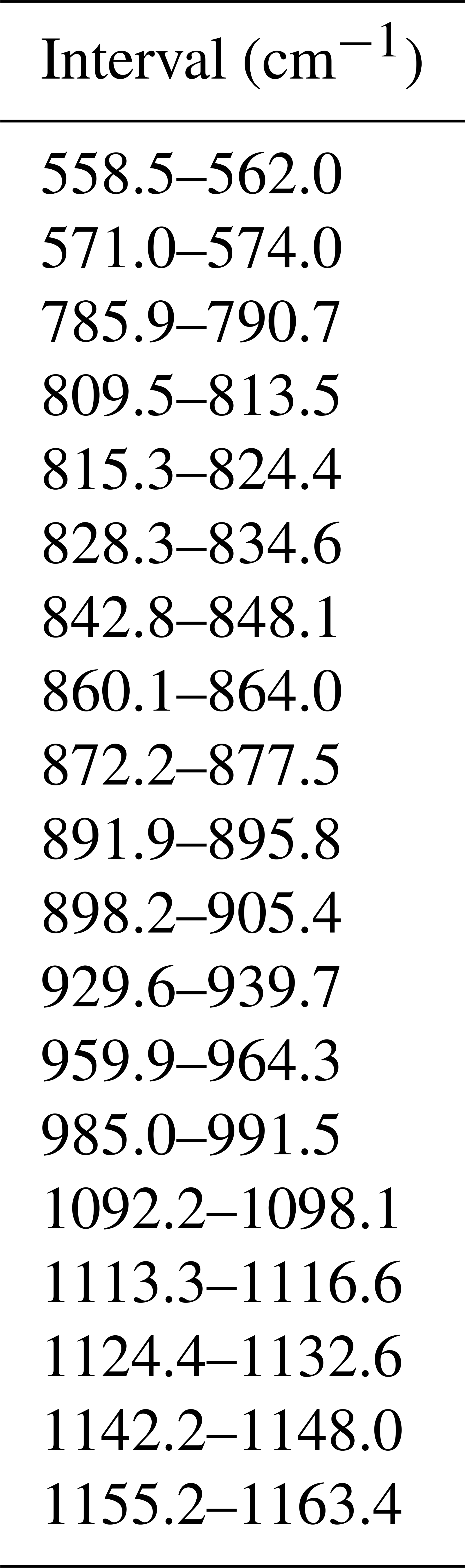
Table B1 Microwindows used in TCWret to retrieve the microphysical cloud parameters of this dataset.

The aim of the iterations is to minimize the cost function ξ²(x).

$$\begin{array}{}\text{(B4)}& \begin{array}{rl}{\mathit{\xi }}^{\mathrm{2}}\left({\mathit{x}}_n\right)& ={\left[\mathit{y}-F\left({\mathit{x}}_n\right)\right]}^T{\mathbf{S}}_y^{-\mathrm{1}}\left[\mathit{y}-F\left({\mathit{x}}_n\right)\right]\\ & +{\left[{\mathit{x}}_{\mathrm{a}}-{\mathit{x}}_n\right]}^T{\mathbf{S}}_{\mathrm{a}}^{-\mathrm{1}}\left[{\mathit{x}}_{\mathrm{a}}-{\mathit{x}}_n\right]\end{array}\end{array}$$

Convergence is reached if the change in the cost function is below a given threshold, here set to 0.1 %:

$$\begin{array}{}\text{(B5)}& {\displaystyle \frac{{\mathit{\xi }}^{\mathrm{2}}\left(x_{n+\mathrm{1}}\right)-{\mathit{\xi }}^{\mathrm{2}}\left(x_n\right)}{{\mathit{\xi }}^{\mathrm{2}}\left(x_{n+\mathrm{1}}\right)}}<\mathrm{0.001}.\end{array}$$

However, convergence in the sense of the cost function does not necessarily mean that the fitted and measured spectra match. For example, the step size parameter of the Levenberg–Marquardt method could be so large that the cost function changes little. Then the convergence criterion is fulfilled, but the fit does not agree with the measurement. To identify these cases, a reduced-χ² test is performed. This test is used to calculate the distance between calculated and measured radiance, taking into account the variance of the spectrum σ². It is defined as

$$\begin{array}{}\text{(B6)}& {\displaystyle }{\mathit{\chi }}_{\mathrm{reduced}}^{\mathrm{2}}={\displaystyle \frac{\mathrm{1}}{\text{DOF}}}\cdot \sum _{m=\mathrm{1}}^N{\displaystyle \frac{y\left({\overline{\mathit{\nu }}}_{\mathrm{m}}\right)-F(\mathbf{x},{\overline{\mathit{\nu }}}_{\mathrm{m}})}{{\mathit{\sigma }}^{\mathrm{2}}}},\end{array}$$

with DOF equal to the number of data points minus the number of parameters. The microwindow is denoted as ${\overline{\mathit{\nu }}}_{\mathrm{m}}$. As empirical values, we assume that all retrievals with ${\mathit{\xi }}_{\mathrm{reduced}}^{\mathrm{2}}<\mathrm{1.0}$ converged correctly. Results with ${\mathit{\tau }}_{\mathrm{liq}}+{\mathit{\tau }}_{\mathrm{ice}}>\mathrm{6}$ are excluded.

As we do not necessarily have prior information about the optical depths and effective radii, we decided to set the covariance of the a priori to large values. This ensures that the chosen a priori does not constrain the retrieval too strongly. Initial values and the a priori are set to equal values: ${\mathit{x}}_{\mathrm{a}}=(\mathrm{0.25},\mathrm{0.25},\log (\mathrm{5.0}),\log (\mathrm{20.0}\left)\right)$. The logarithm was chosen so that all entries of x_a have similar sizes. The variance–covariance matrix of the a priori is set to

$$\begin{array}{}\text{(B7)}& {\displaystyle }{\mathbf{S}}_{\mathrm{a}}^{-\mathrm{1}}=\left(\begin{array}{cccc}\mathrm{0.04}& \mathrm{0}& \mathrm{0}& \mathrm{0}\\ \mathrm{0}& \mathrm{0.04}& \mathrm{0}& \mathrm{0}\\ \mathrm{0}& \mathrm{0}& \mathrm{0.047}& \mathrm{0}\\ \mathrm{0}& \mathrm{0}& \mathrm{0}& \mathrm{0.047}\end{array}\right).\end{array}$$

The values in x_a and ${\mathbf{S}}_{\mathrm{a}}^{-\mathrm{1}}$ are chosen empirically. Since initially no information about the cloud parameters is available, x_a and ${\mathbf{S}}_{\mathrm{a}}^{-\mathrm{1}}$ should not restrict the retrieval too much. Therefore, the variances in ${\mathbf{S}}_{\mathrm{a}}^{-\mathrm{1}}$ are set to large values.

Variances in ${\mathbf{S}}_y^{-\mathrm{1}}$ are calculated from the spectral region between 1925 and 2000 cm⁻¹, where no signal from the atmosphere is expected. The variance–covariance matrix is assumed to be diagonal: S_y=σ²I. It is assumed to be the variance of the scene. To retrieve cloud parameters, only radiance from spectral intervals given in Table B1 is used. The variances of S_y propagated into the covariance matrix S_r of the result by applying a transfer matrix T. In each step T is calculated taking into account the current step size parameter μ by

$$\begin{array}{}\text{(B8)}& {\displaystyle }\left\{\begin{array}{l}{\mathbf{T}}_{\mathbf{0}}=\mathbf{0}\\ {\mathbf{T}}_{i+\mathrm{1}}={\mathbf{G}}_i+\left(\mathbf{I}-{\mathbf{G}}_i{\mathbf{K}}_i-{\mathbf{M}}_i{\mathbf{S}}_a^{-\mathrm{1}}\right){\mathbf{T}}_i,\end{array}\right.\end{array}$$

with 0 as the zero matrix and I as the identity matrix. M_i is the inverse of the term in the parentheses on the left side of Eq. (B3), and ${\mathbf{G}}_i={\mathbf{M}}_i{\mathbf{K}}_i^T{\mathbf{S}}_y^{-\mathrm{1}}$. Diagonal elements of S_r are the variances of the final cloud parameters.

Appendix C: Retrieval performance on simulated spectra

A set of simulated test cases containing spectral radiances of artificial clouds with known cloud parameters, created by Cox et al. (2016), will be used to test the ability of TCWret to retrieve τ_liq, τ_ice, r_liq and r_ice. Additionally, the derived quantities LWP and IWP are discussed. This dataset contains several representative cases of Arctic clouds. Clouds are set to be vertically homogeneous, topped by a layer of liquid water or with thin boundaries. Ice crystal shapes are mostly set to be spheres, but some cases were calculated with hollow columns, solid columns, bullet rosettes or plates. All spectra are convoluted with a sinc function to the resolution of the IFS 55 Equinox (0.3 cm⁻¹) and perturbed by a Gaussian-distributed noise of $\mathrm{1}\mathrm{mW}({\mathrm{m}}^{\mathrm{2}}\mathrm{sr}{\mathrm{cm}}^{-\mathrm{1}}{)}^{-\mathrm{1}}$: we modified the spectral radiance at each wavenumber by drawing a random number from a normal distribution with the true spectral radiance as the mean of the distribution and $\mathrm{1}\mathrm{mW}({\mathrm{m}}^{\mathrm{2}}\mathrm{sr}{\mathrm{cm}}^{-\mathrm{1}}{)}^{-\mathrm{1}}$ as its standard deviation. This value has been chosen because it is near the observed standard deviation of the real spectra from the measurement campaign of $\mathrm{0.82}\mathrm{mW}({\mathrm{m}}^{\mathrm{2}}\mathrm{sr}{\mathrm{cm}}^{-\mathrm{1}}{)}^{-\mathrm{1}}$. Ice crystals are chosen to be spheres; thus only the test cases which are calculated with spherical ice crystals are used here. The influence of the chosen ice particle form will be addressed later.

Table 3 gives the correlation coefficients, mean biases and standard deviations between the retrieved cloud parameters of the test cases and the true cloud parameters. Additionally, the standard deviations calculated via the variance–covariance matrix are given. TCWret is able to determine optical depths and effective radii of the simulated spectra.

Of all direct retrieval products, the optical depths τ_liq and τ_ice have the highest agreement with the true cloud parameters. For the liquid phase, the difference from the true optical depths is $(-\mathrm{0.1}\pm \mathrm{0.5})$. For the optical depth of the ice phase, the difference is larger with (0.2±0.6). Since τ_liq and τ_ice include both optical depths and phase, the optical depth of the condensed water ${\mathit{\tau }}_{\mathrm{cw}}={\mathit{\tau }}_{\mathrm{liq}}+{\mathit{\tau }}_{\mathrm{ice}}$ as well as the fraction of ice in the optical depth $f_{\mathrm{ice}}={\mathit{\tau }}_{\mathrm{ice}}\cdot {\mathit{\tau }}_{\mathrm{cw}}^{-\mathrm{1}}$ are calculated. Here it becomes clear that the optical depth can be determined accurately ($\left|r\right|=\mathrm{0.99}$, mean bias and RMSE (0.1±0.2)). It then also follows that the deviations of τ_liq and τ_ice come from the phase determination. The deviation for the phase is (0.1±0.3) with a correlation coefficient of $\left|r\right|=\mathrm{0.70}$.

When considering the effective radii, only results of r_liq were used where f_ice is less than 0.9. For r_ice only results with f_ice>0.1 are considered. The mean difference in the retrieval from the true parameters and the root-mean-square error are $(-\mathrm{2.4}\pm \mathrm{4.1})$ for r_liq and (3.0±10.0) for r_ice.

To estimate the influence of the a priori on the calculated result, the averaging kernel matrix is used. The mean averaging kernel matrix over all retrievals is

$$\begin{array}{}\text{(C1)}& {\displaystyle }\mathbf{A}=\left(\begin{array}{cccc}\mathrm{0.87}& \mathrm{0.09}& -\mathrm{0.15}& -\mathrm{0.09}\\ \mathrm{0.11}& \mathrm{0.90}& \mathrm{0.19}& \mathrm{0.03}\\ -\mathrm{0.04}& \mathrm{0.07}& \mathrm{0.50}& \mathrm{0.05}\\ -\mathrm{0.16}& \mathrm{0.05}& \mathrm{0.03}& \mathrm{0.42}\end{array}\right).\end{array}$$

From Eq. (8) it can be seen that the diagonal elements show for each parameter how strongly the retrieved parameter is influenced by the a priori. Whereas the diagonal elements of the optical depths are near 1, indicating independence from the a priori, results for r_liq and r_ice show a larger influence from the a priori. From the trace of the averaging kernels follow 2.69 degrees of freedom of the signal.

The water paths are calculated from the optical depths and effective radii; therefore both quantities are influenced by the phase determination, as seen before in τ_liq,ice and r_liq,ice. The difference from the test cases is $(-\mathrm{1.6}\pm \mathrm{6.3})$ for the LWP and (1.9±10.0) for the IWP. However, the RMSE for the LWP is less than the minimum RMSE observed for the LWP from microwave radiometer of at least 15 g m⁻² (Löhnert and Crewell, 2003).

Standard deviations given by the variance–covariance matrix of the retrieval are shown in Table 3 and named ERR(OE). ERR(OE) is below RMSE for τ_liq,ice, r_liq,ice, the LWP and the IWP. This might be due to uncertainties from the forward model – which are neglected here – propagated into the retrievals or due to the assumption of a diagonal variance matrix S_y. To compensate for these effects, the uncertainties from the posterior covariance matrix are scaled by RMSE $/$ ERR(OE) with the RMSE from Table 3 for the discussion in Sect. 5.

Table C1 Determination of r_liq depending on the cloud phase.

Table C2 Determination of r_ice depending on the cloud phase.

C1 Mean bias and RMSE of effective radii

In the previous section, the results for r_liq and r_ice were only considered for a certain range of f_ice. Thus, liquid drops were only included in the consideration if the ice content was not higher than 90 %. For ice crystals, the limit was at least 10 % ice content. In the following, these limits are shifted so that the results go in the direction of a single-phase retrieval for liquid water and ice.

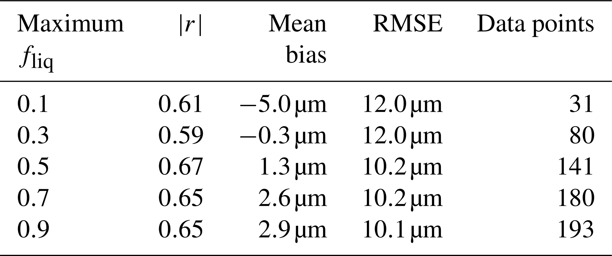
Table C1 shows the results for liquid water. The entries at the top describe cases with a higher proportion of liquid water than the cases at the bottom, which allow a higher proportion of ice. They are cumulative, which means that each record also contains the data of the record above it. From the test cases it follows that the fewer ice crystals present, the lower the RMSE. Also, the absolute mean bias decreases with lower ice content up to an ice content between 10 % and 30 %. These results indicate that the presence of ice crystals lead to an underestimation of r_liq by TCWret.

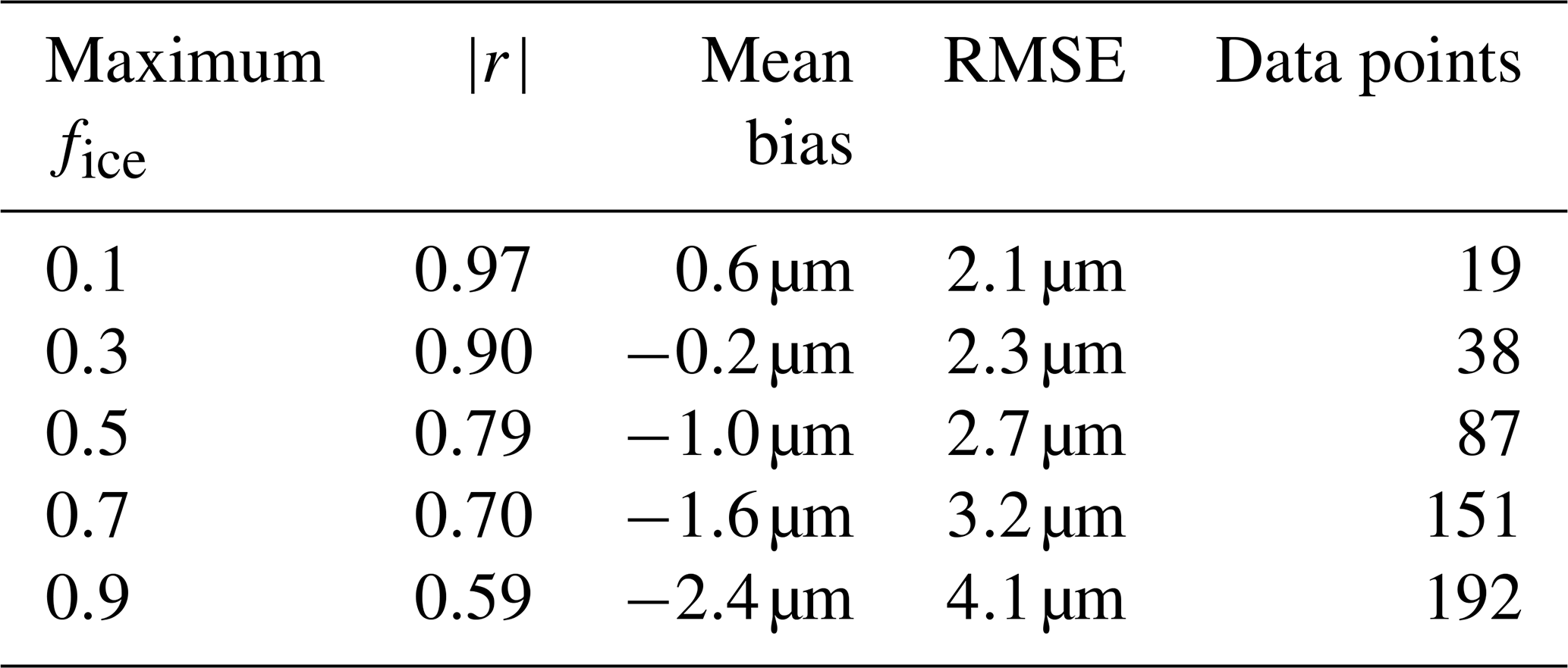
Table C2 show the results for ice crystals. Here we introduced f_liq, which is defined as $f_{\mathrm{liq}}=\mathrm{1}-f_{\mathrm{ice}}$, to create a table consistent with Table C1. Here one can see that the RMSE of r_ice is almost independent of the water content. However, there is a dependence of the mean bias on water content. While removing clouds with very high water content leads to a decrease in absolute mean bias, the absolute value of mean bias increases for clouds with high ice content, so TCWret underestimates r_ice of the simulated spectra.

Appendix D: Influence of trace gas concentrations on the retrieval

In the LBLRTM, a standard atmosphere was used for gases except water vapor. Therefore, the concentration of CO₂ is set to 330 ppm, although the real concentration in summer 2017 is about 410 ppm. To investigate the influence of an incorrect trace gas concentration, retrievals from the 11 June 2016 have been performed with both atmospheric concentrations of CO₂. Differences are calculated for the cloud parameters τ_liq, τ_ice, r_liq and r_ice and shown in Fig. D1. For all parameters, correlation coefficients between $\left|r\right|=\mathrm{0.98}$ and $\left|r\right|=\mathrm{1.00}$ can be observed. The maximum mean bias is observed for r_liq (0.1 µm), and the maximum RMSE is observed for r_ice (1.3 µm). From this it can be concluded that the influence of the trace gas concentration is negligible compared to the other uncertainties.

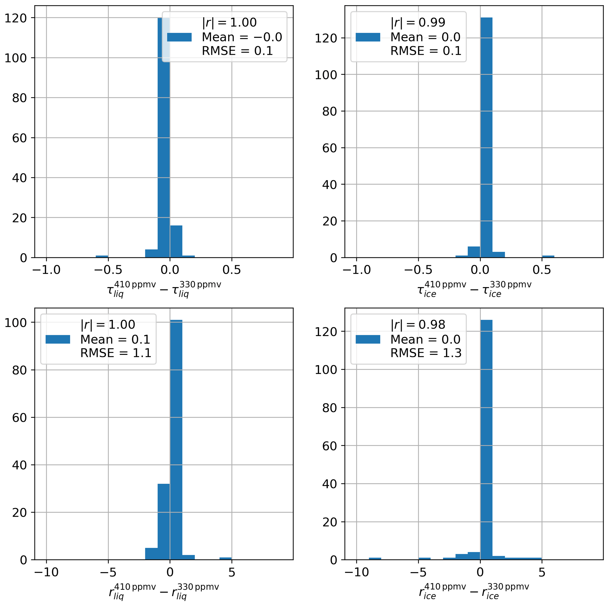
Figure D1 Histograms of differences for CO₂ concentrations of 410 and 330 ppm for τ_liq, τ_ice, r_liq and r_ice.

Appendix E: Ice crystal shapes in the netCDF file

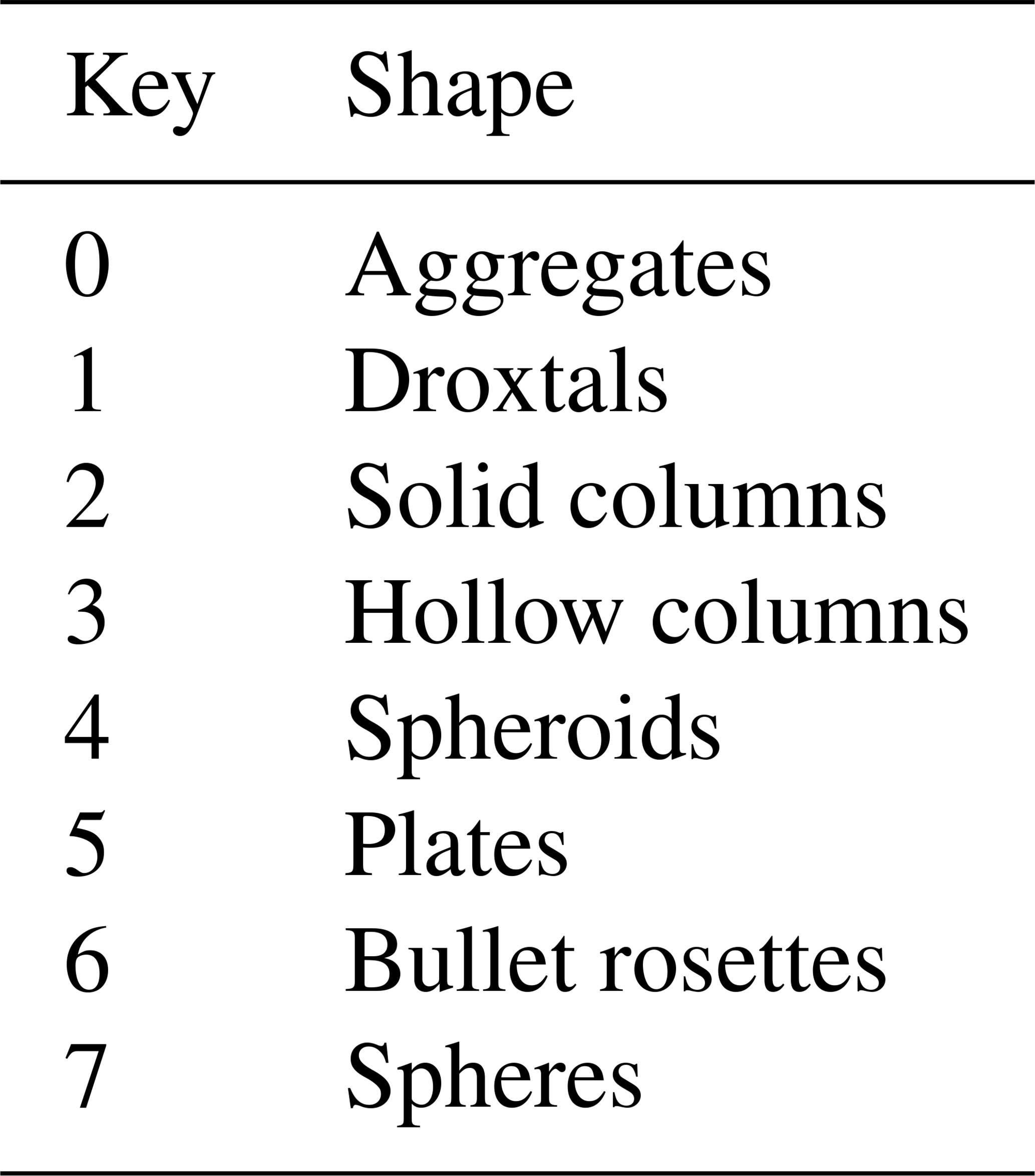
Table E1 refers to each key in the field ice_shape in the netCDF file and the corresponding ice crystal shape.

Table E1 Ice crystal shapes in the netCDF file and the corresponding number.