A 1 km daily surface soil moisture dataset of enhanced coverage under all-weather conditions over China in 2003–2019

Surface soil moisture (SSM) is crucial for understanding the hydrological process of our earth surface. The passive microwave (PM) technique has long been the primary tool for estimating global SSM from the view of satellites, while the coarse resolution (usually $>\sim \mathrm{10}$ km) of PM observations hampers its applications at finer scales. Although quantitative studies have been proposed for downscaling satellite PM-based SSM, very few products have been available to the public that meet the qualification of 1 km resolution and daily revisit cycles under all-weather conditions. In this study, we developed one such SSM product in China with all these characteristics. The product was generated through downscaling the AMSR-E/AMSR-2-based (Advance Microwave Scanning Radiometer of the Earth Observing System and its successor) SSM at 36 km, covering all on-orbit times of the two radiometers during 2003–2019. MODIS optical reflectance data and daily thermal-infrared land surface temperature (LST) that had been gap-filled for cloudy conditions were the primary data inputs of the downscaling model so that the “all-weather” quality was achieved for the 1 km SSM. Daily images from this developed SSM product have quasi-complete coverage over the country during April–September. For other months, the national coverage percentage of the developed product is also greatly improved against the original daily PM observations through a specifically developed sub-model for filling the gap between seams of neighboring PM swaths during the downscaling procedure. The product compares well against in situ soil moisture measurements from 2000+ meteorological stations, indicated by station averages of the unbiased root mean square difference (RMSD) ranging from 0.052 to 0.059 vol vol⁻¹. Moreover, the evaluation results also show that the developed product outperforms the SMAP (Soil Moisture Active Passive) and Sentinel (active–passive microwave) combined SSM product at 1 km, with a correlation coefficient of 0.55 achieved against that of 0.40 for the latter product. This indicates the new product has great potential to be used by the hydrological community, by the agricultural industry, and for water resource and environment management. The new product is available for download at https://doi.org/10.11888/Hydro.tpdc.271762 (Song and Zhang, 2021b).

1 Introduction

Surface soil moisture (SSM) is one of the most important variables that dominate the mass and energy cycles of the earth surface system (Entekhabi et al., 2010b). Satellite-based SSM datasets of sufficiently fine spatiotemporal resolutions over large-scale areas have significant implications for improved investigations in various research fields including hydrological signature identification (Zhou et al., 2021; Jung et al., 2010), agricultural yield production estimation (Ines et al., 2013; Pan et al., 2019), drought/waterlogging monitoring and warning (Vergopolan et al., 2021; Den Besten et al., 2021; Jing and Zhang, 2010), and weather prediction and future climate analysis (Koster et al., 2010; Walker and Houser, 2001). Microwave bands with centimeter-sized or longer wavelengths (X-band, C-band, and L-band) are currently identified as the primary band channels suitable for SSM observations from the view of satellites due to their high penetration capabilities through cloud layers and vegetation canopies. In terms of sensor types, microwave SSM detection includes passive microwave (radiometer-based) techniques and active microwave (radar, scatterometer) techniques. Satellite-based passive microwave (PM) radiometers, e.g., Soil Moisture Active Passive (SMAP), Soil Moisture and Ocean Salinity (SMOS), and the Advance Microwave Scanning Radiometer-2 (AMSR-2), can obtain SSM observations at a revisit interval of 1–3 d, with relatively poor native spatial resolutions of tens of kilometers. Active microwave (AM) such as radar can achieve kilometer-scale and even finer resolutions of observations targeting the earth surface. However, this usually sacrifices the swath width of radar configuration, because of which most satellite-based synthetic aperture radars (SARs) have an obviously longer global revisit cycle (usually longer than 5 d, e.g., Sentinel-1 SAR data) than the typical radiometers. Moreover, AM radar backscatter signals are extremely sensitive to speckle noise (Entekhabi et al., 2016), as well as the influence from soil roughness, vegetation canopy structure, and water content (Piles et al., 2009). All the above influential factors have seriously impeded the use of AM radar techniques or combination of passive–active microwave datasets for producing high-spatial-resolution SSM products with a frequent revisit.

Apart from microwave signals, solar reflectance or ground emission signals originating from optical and infrared band domains also have the potential to reflect SSM variation. Based on optical and infrared bands, however, SSM is typically estimated based on indirect relationships through intermediate variables like soil evaporation (Komatsu, 2003), vegetation condition (Zeng et al., 2004), or soil thermal inertia (Verstraeten et al., 2006). To overcome the spatiotemporally instable performance in SSM modeling that might be brought by such indirect relationships, they are typically fused with the PM SSM datasets. In this manner, it can reconcile the advantage of PM observations well with respect to its high sensitivity to SSM variation, as well as that of optical and infrared observations with respect to its finer spatial resolutions at kilometer or even hectometer scales. Such data fusion techniques are also known as downscaling techniques of PM remote sensing SSM. Archetypal downscaling models include the models based on the universal triangle feature space (UTFS) (Chauhan et al., 2003; Choi and Hur, 2012; Sanchez-Ruiz et al., 2014), the DISaggregation based on a Physical And Theoretical scale CHange (DISPACTH) model (Merlin et al., 2010, 2005, 2013, 2008), and the University of California Los Angeles (UCLA) model (Peng et al., 2016). The physics of these models are mainly based on the response of SSM variation to changes in soil evaporation or land surface evapotranspiration. Another significant branch of such downscaling models is based on the sensitivity of SSM to soil thermal inertia, which is quantified by diurnal land surface temperature (LST) difference estimated from thermal-infrared wave bands (Fang and Lakshmi, 2013; Fang et al., 2018).

Sabaghy et al. (2020) have shown that using optical and infrared data can achieve finer-resolution SSM estimates which are more consistent with ground soil moisture records compared with using the radar datasets. Moreover, considering the short revisit cycle (daily) of optical and infrared sensors on board typical polar-orbit satellites, using optical and infrared datasets to downscale PM SSM should be among the optimal methods for obtaining SSM data with high spatiotemporal resolutions over national, continental, or global scales. On the other hand, satellite remote sensing SSM products that are characterized by 1 km resolution of daily revisit intervals and stable, long time series dating back to at least 15–20 years ago are urgently required for accelerating the development of various research fields, especially the agriculture industry, water resources management, and hydrological disaster monitoring (Sabaghy et al., 2020; Mendoza et al., 2016). However, very seldom are sets of such data products publicly available to the remote sensing research community because of the following drawbacks. First, there is a serious lack of cloud-free optical and infrared imagery, which means the method cannot deliver any SSM downscaling under cloudy/rainy weather. Second, most of the above-mentioned optical and infrared data-based downscaling methods were mainly evaluated at regional or even smaller scales. This might raise concern on the universality of those methods. For example, the DISPATCH method has been recognized to be less effective in humid (energy-limited) regions compared with in arid and semi-arid (water-limited) regions (Molero et al., 2016; Song et al., 2021; Zheng et al., 2021). As far as the UTFS-based method is concerned, a poorer performance was obtained compared to the DISPATCH in a typical water-limited region in North America, according to the experiment conducted by Kim and Hogue (2012).

To improve the above-mentioned issues, we produced an all-weather daily SSM data product at 1 km resolution all over China during 2003–2019, based on the fusion of multiple remote sensing techniques, including reconstruction of optical and infrared observations under cloudy weather, as well as an improved PM SSM downscaling methodology proposed in our previous study (Song et al., 2021). The potential significance of this study includes

1. better serving and investigating the land surface hydrology processes and their sophisticated interactions with human society at multi-scale (from national to regional) resolutions in China because the country covers about $\mathrm{1}/\mathrm{15}$ of the global terrestrial area with about $\mathrm{1}/\mathrm{5}$ of the world population, and

2. providing a methodology framework that can inspire future studies on generating similar SSM datasets all over the globe, based on the plentifulness of resources on climate type, land covers, and topography in China.

2 Methods and materials

2.1 Datasets

2.1.1 PM SSM data

Spatial downscaling of PM SSM is the fundamental theory for constructing the target finer-resolution data product in this study. Therefore, the native retrieval accuracy of the coarse-resolution PM SSM data product, based on which the downscaling procedures are performed, is considerably crucial to the performance of the downscaled data product (Busch et al., 2012; Im et al., 2016; Kim and Hogue, 2012). Although the L-band PM brightness temperature (TB) observed by satellite missions such as SMAP or SMOS is considered more suitable for SSM retrieval compared with C- or X-band TB, both above missions started their space operations in the 2010s. This means that to obtain downscaled SSM of longer historical periods, we are still required to rely on other C-/X-band-based radiometers which started their operations earlier than SMAP and SMOS. An optimal satellite PM TB observation system dating back to earlier years of this century is composed of the Advanced Microwave Scanning Radiometer of the Earth Observing System (AMSR-E), together with its successor AMSR-2. AMSR-E operated during 2002–2011 on board the Aqua satellite which is operated by the National Aeronautics and Space Administration (NASA), whilst AMSR-2 has been operating on board the Global Change Observation Mission 1 Water (GCOM-W1) satellite developed by the Japan Aerospace Exploration Agency (JAXA) since 2012.

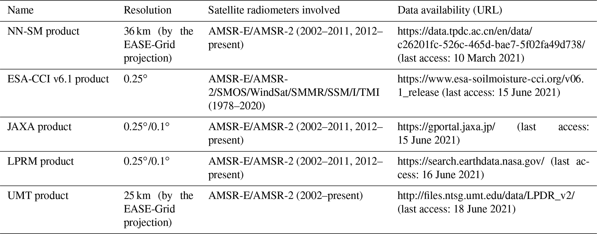
Several classical PM SSM retrieval algorithms have been applied to the aforementioned AMSR series (including AMSR-E and AMSR-2) TB for generating long-term global SSM products at 25 km (Table 1), including the JAXA algorithm (Fujii et al., 2009; Koike et al., 2004), the Land Parameter Retrieval Model (LPRM) algorithm (Song et al., 2019b; Meesters et al., 2005; Owe et al., 2001), and the algorithm developed by the University of Montana (UMT) (Jones et al., 2009; Du et al., 2016). A recent AMSR-based nighttime SSM product during 2002–2019 has been produced through a neural network trained against SMAP radiometer-based descending SSM (hereafter referred to as “NN-SM product”) (Yao et al., 2021). The global validation results show that this NN-SM product is better than the JAXA and LPRM products.

Moreover, the NN-SM has also been compared with another long-term ∼25 km all-weather SSM dataset generated through the European Space Agency (ESA)'s Climate Change Initiative (CCI) program. The ESA-CCI SSM product is different from the products mentioned above in that it was implemented through the fusion of observations from comprehensive AM- and PM-based satellite sensors rather than only relying on the radiometers of the AMSR series. According to Yao et al. (2021), the ESA-CCI SSM has slightly better validation accuracy than the NN-SM product, but the number of available observations per pixel cell in an entire year is much smaller for the ESA-CCI SSM in Southeast China. In view of all of the above coarse-resolution SSM data products, we finally selected the NN-SM product to implement the following spatial downscaling procedures rather than the ESA-CCI SSM to make a balance between data accuracy and data availability per year. We have also made additional evaluations within China in Appendix A to ensure the relatively outstanding performance of the NN-SM product as described above.

Table 1 Information of all-weather microwave remote sensing coarse-resolution SSM data products that can be potentially downscaled to obtain fine-resolution SSM.

2.1.2 Optical remote sensing data and digital elevation model (DEM)

Optical remote sensing datasets provide finer spatial texture information on the daily basis for the downscaling purpose of PM SSM. Such data that can be used as inputs of our SSM product processing line are mainly provided by the Moderate-resolution Imaging Spectroradiometer (MODIS) on board the Terra and Aqua satellites. Specifically, they involve the 1 km daily nighttime Aqua MODIS LST product (MYD21A1N.v061) and the 500 m daily Bidirectional Reflectance Distribution Function (BRDF) – Adjusted Reflectance dataset (MCD43A4.v061). MYD21A1 LST data can be recognized as a crucial proxy of land surface thermal capacity (Fang et al., 2013) and soil evaporative rate (Merlin et al., 2008). The MCD43A4 nadir reflectance product, with view angle effect corrected using the BRDF model, is capable of providing observations from visible to shortwave infrared bands that can characterize water content variation in the bare soils as well as the vegetation canopy. Overall, the above-mentioned datasets were selected primarily because they deliver indicators (land surface thermal capacity, soil evaporative rate, or vegetation condition) that can respond well to soil moisture dynamics from different aspects. Prior to being employed for SSM downscaling, a conventional pre-processing procedure of pixel quality check was applied for both optical products by screening out pixels not classed as “good quality”, according to the 8 bit quality assessment (QA) field of each spectral band. Moreover, to normalize their natively different spatial resolutions, all MCD43A4-based reflectance values at the 500 m pixel level were upscaled to the sinusoidally projected MODIS 1 km grids using their spatial averages.

Apart from MODIS optical remote sensing data, all 90 m DEM tiles generated by the NASA Shuttle Radar Topography Mission (SRTM; http://srtm.csi.cgiar.org/, last access: 10 July 2020) were mosaicked all over China and then employed as another essential input variable for the procedures as described in Sect. 2.2.2 below. Similar to that applied to the MCD43A4 product, spatial upscaling in correspondence to the MODIS 1 km grids is also an indispensable pre-processing step for the mosaicked DEM data.

2.1.3 Study area and validation data

Our study area is set up as the total terrestrial extent of China. To comprehensively evaluate the SSM downscaling performances for different geographic regions (see Sect. 3.3), we divided the country further into six different geographic–climate regions using elevation, precipitation, hydrogeology, vegetation type, and topography. The six regions include the northeast monsoon (NEM) region, the northwest arid (NWA) region, the Qinghai–Tibet Plateau (QTP) region, the North China Monsoon (NCM) region, the South China Monsoon (SCM) region, and the southwest humid (SWH) region. The detailed delimitation principle of these geographic–climate regions was originally described in Meng et al. (2021). The geographic zoning map is shown in Fig. 1, while the corresponding shapefile boundary files can be accessed from the Resource and Environment Science and Data Center of the Chinese Academy of Sciences (http://www.resdc.cn/, last access: 22 May 2021).

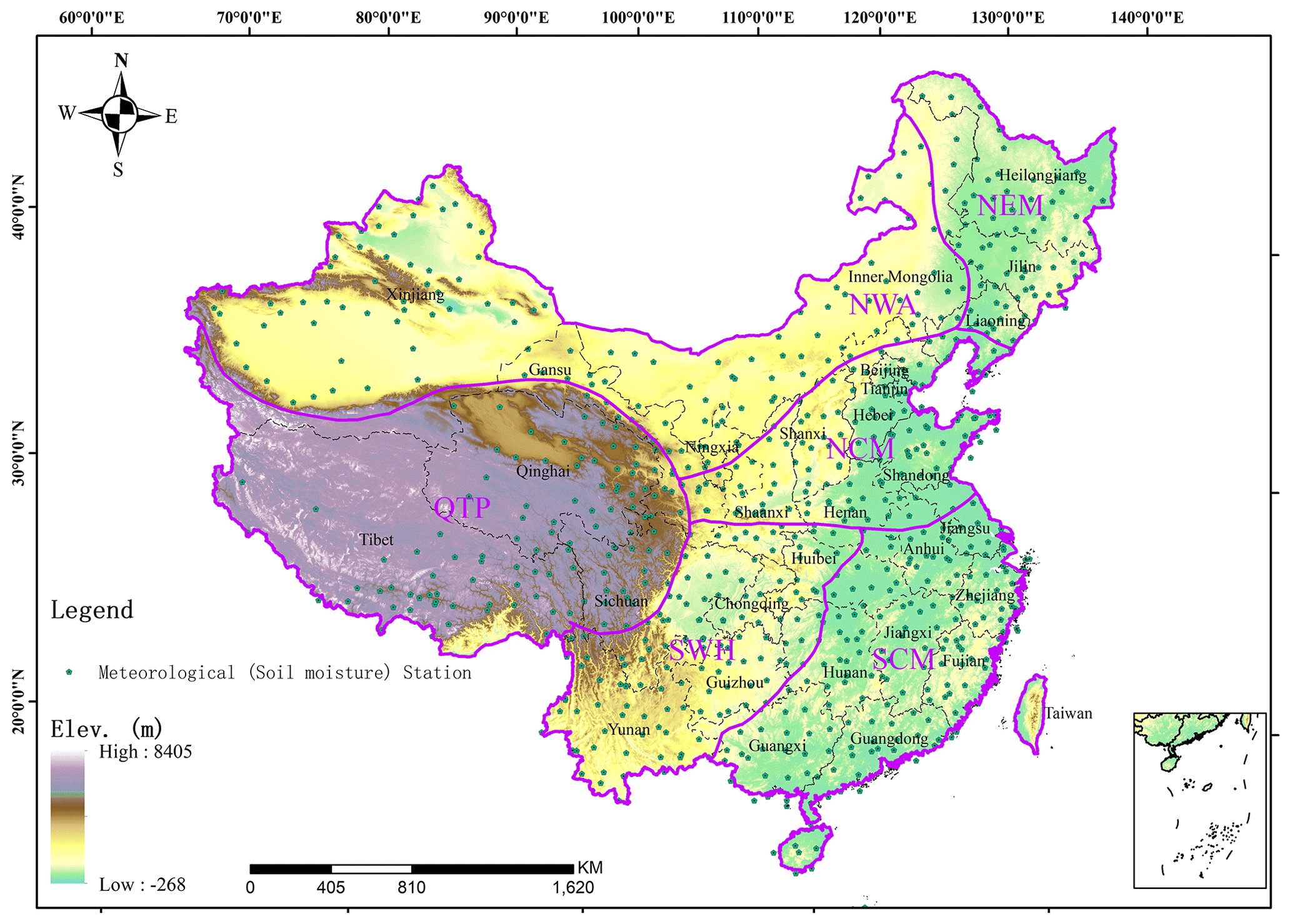
Figure 1 The geographic zoning map of the study area (delineated using the purple color) superposed with topographic information, as well as general locations for the 756 basic meteorological stations (http://data.cma.cn/, last access: 20 January 2021) that provide partial benchmark measurements for SSM and LST validation in this study.

We utilized ground soil moisture measurements for validating the downscaled remote sensing SSM product at the local scale. The ground measurements are derived from 2417 meteorological stations (including 756 basic stations of the National Climate Observatory and 1661 regionally intensified stations) in China, as partially shown in Fig. 1. The soil moisture measurement devices at these stations, with uniform observation standards, are instrumented under the national project of the Operation Monitoring System of Automatic Soil Moisture Observation Network in China (Wu et al., 2014 ), the construction of which has been led by the China Meteorological Administration since 2005. Until 2016, all stations were in operation for automatically observing hourly in situ soil moisture dynamics at eight different depth ranges (0–10, 10–20, 20–30, 30–40, 40–50, 50–60, 70–80, 90–100 cm). It has also been widely used by previous studies for evaluating satellite soil moisture estimates in China (Meng et al., 2021; Chen et al., 2020; Zhang et al., 2014; Zhu and Shi, 2014). In our current study, ground measurements matching the shallowest depth range (0–10 cm) from the initial time of each station until the end of 2019 are employed as the validation benchmark of the satellite SSM retrievals. At the temporal dimension, measurements made at 01:00 and 02:00 LT are averaged, in order to match the mean satellite transit time of 01:30 LT for AMSR descending observations.

Moreover, 0 cm top ground temperatures are simultaneously measured at all these meteorological stations on the daily basis at the local time windows of 02:00, 10:00, 14:00, and 22:00 LT (local time). We therefore exploited such measurements recorded at 02:00 LT to validate the cloud gap-filled nighttime (∼01:30 LT) LST estimates over the Aqua-MODIS-based 1 km pixels containing these stations (see Sect. 2.2.2). Our primary validation period covers the entire years of 2017, 2018, and 2019.

In addition to the ground soil moisture measurements, the SMAP level 3 radiometer-based daily 36 km SSM product (https://doi.org/10.5067/OMHVSRGFX38O; O'Neill et al., 2021b) in its descending orbit scenes (at ∼06:00 LT) from 2016 to 2019, was employed as another complemental validation benchmark. This dataset has the potential to provide more comprehensive evaluations to our developed product at regional/national scales, especially on account of its notably creditable performance (see Fig. A1 in Appendix A). The latest version of this dataset (SPL3SMP, Version 8) contains soil moisture retrievals based on different algorithms including the dual channel algorithm and the single channel algorithm. In this study we only extracted SSM estimates derived with the dual channel algorithm because this algorithm was reported to outperform the single channel algorithm over some agricultural cropland core validation sites (O'Neill et al., 2021a).

2.1.4 Ancillary SSM products for comparison

In order to comprehensively demonstrate the validation performance of our proposed SSM product, there is necessity to make an inter-comparison against similar existing datasets. In this regard, we introduced the level 2 SMAP–Sentinel active–passive combined SSM product on 1 km earth-fixed grids, i.e., the SPL2SMAP_S_V3 dataset (Das et al., 2020), and used its validation performance against in situ measurements throughout the years of 2017, 2018, and 2019 as a baseline to better evaluate our proposed SSM product. The SPL2SMAP_S_V3 dataset contains global SSM at resolutions of 3 and 1 km, which were disaggregated from the SMAP radiometer-based SSM retrievals of 36 and 39 km footprints in conjunction with the high-resolution Sentinel-1 C-band radar backscatter coefficients (Das et al., 2019). To our knowledge, this dataset is possibly the only publicly available product which can provide global remote sensing SSM estimates at the 1 km resolution. The Sentinel backscatter coefficient inputs for this product are only those received in the descending orbit scenes (at ∼06:00 LT), whilst the closest SMAP SSM retrievals from either ascending (at ∼18:00 LT) or descending orbits are used to spatially match up with the Sentinel-1 scene. It is noticed that at the descending observation time the soil moisture vertical profile has approached a hydrostatic balance (Montaldo et al., 2001), thereby providing the optimal chance for soil moisture fusion and validation with observations at different soil depths. Therefore, we only selected the 1 km disaggregated SSM estimates based on descending SMAP SSM retrievals (i.e., the subset with the field name of “disagg_soil_moisture_1 km” in the SPL2SMAP_S_V3 dataset). Meanwhile, the 0–10 cm in situ soil moisture measurements observed at 06:00 LT and the SMAP radiometer-based descending SSM estimates were employed as the validation benchmarks in a manner similar to that applied to our proposed SSM product (Sect. 2.1.3).

2.2 Methodology

The general methodological framework for producing the all-weather daily 1 km SSM product is shown in Fig. 2, with details described in the following context of this section.

Figure 2 The overall methodological framework of this study.

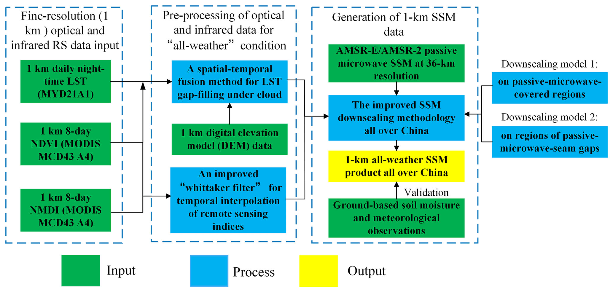
2.2.1 Reconstruction of thermal-infrared LST and remote sensing (vegetation) indices under cloudy conditions

Reconstruction of missing pixels under cloudy conditions in the optical remote sensing input datasets is the prerequisite for achieving the “all-weather” property of the final downscaled SSM output. For reconstructing thermal-infrared LST, we adopted the cloud gap-filling method as proposed by our previous study (Song et al., 2019a). This method, also referred to as a typical spatiotemporal data fusion (STDF) method (Dowling et al., 2021), was built using clear-sky LST observations of spatially neighboring pixels observed at proximal dates, with concurrent normalized difference vegetation index (NDVI) and DEM also employed as additional data inputs. The STDF method can be expressed as follows:

$$\begin{array}{}\text{(1)}& {\text{LST}}_{t_{\mathrm{1}}}^{\ast }=a\times {\text{LST}}_{t_{\mathrm{0}}}^{\ast }+b\times {\text{NDVI}}_{t_{\mathrm{1}}}^{\ast }+c\times {\text{DEM}}^{\ast }+d,\end{array}$$

where the superscript ^∗ indicates that this variable has been normalized to the range 0 to 1.0 (Song et al., 2019a), based on the maximum and minimum values of that variable found across China (excluding invalid values representing states of snow, ice, and water bodies). Parameters a, b, c, and d are coefficients fitted between all pixels with clear-sky LST estimates on a specific date t₁ (LST${}_{t\mathrm{1}}^{\ast }$) and their counterparts on one proximal date t₀ (LST${}_{t\mathrm{0}}^{\ast }$). NDVI${}_{t\mathrm{1}}^{\ast }$ indicates the corresponding (normalized) NDVI on the t₁ date calculated using the MCD43A4 daily product. After deriving the coefficients of a, b, c, and d, Eq. (1) was used to fill all cloudy MODIS LST pixels on the t₁ date. For any t₁ date included in the study period, the t₀ date was iterated among all neighboring dates of t₁ meeting the condition $|t_{\mathrm{0}}-t_{\mathrm{1}}|\le \mathrm{30}$ (from the nearest date to the furthest date). The average of estimated LST values for t₀ was then taken in which a cloud gap pixel was filled more than once (based on the iterative t₀ dates). The iteration was stopped when the fraction of pixels with effective LST values on t₁ was equal to or exceeded 0.99.

An important flaw of this STDF method should be noted with regard to the potentially existential bias of the cloud gap-filled LST outputs because the outputs represent theoretically reconstructed LST under clear-sky rather than under the real cloudy conditions. Another of our previous studies (Dowling et al., 2021) concerning this STDF method proposed a follow-up step, which incorporated PM-derived surface temperature, to adjust that bias. In our current production pipeline, however, this follow-up step for cloud bias adjustment in LST was not carried out. This is because the results in Appendix B show that using LST generated by the STDF alone leads to more accurate SSM outcomes in general. The possible reasons for this are discussed in Sect. 4.2.

Reconstruction of the remote sensing vegetation indices under cloudy conditions, including NDVI and NMDI (normalized multi-band drought index), was simply based on the modified time series filter of the Whiitaker smoother (MWS) as developed by Kong et al. (2019). This is reasonable because the dynamic trends of vegetation growth are relatively less volatile compared to LST on the daily basis and can thus be gap-filled for missing values using a time-series-filtering-like algorithm.

2.2.2 Improved downscaling technique of SSM based on fusion of PM and optical and infrared data

The core component of the SSM downscaling methodology is an improved linking model between PM SSM and (fine-resolution) optical remote sensing observations. This model enhances the relatively poorer performance of the conventional DISPATCH in energy-limited regions, whilst it maintains the generally good quality of the DISPATCH in water-limited ones. Therefore, the improved model is more appropriate to be applied in China, which contains a wide range of geographical settings, compared to other conventional downscaling models. Since this model originates from our previous study (Song et al., 2021), herein we simply give its mathematical expression as follows:

$$\begin{array}{}\text{(2)}& \text{SSM}={\displaystyle \frac{a\times \ln (\mathrm{1}-\text{SEE})}{\mathrm{1}-b\times \text{NMDI}}}+c.\end{array}$$

In Eq. (2), SEE denotes “soil evaporative efficiency” and is a mathematical function of LST and the typical NDVI, with its specific form described in Merlin et al. (2008). NMDI is another remote sensing index calculated as $\frac{R_{\mathrm{infr},\mathrm{860}\mathrm{nm}}-(R_{\mathrm{sw},\mathrm{1600}\mathrm{nm}}-R_{\mathrm{sw},\mathrm{2100}\mathrm{nm}})}{R_{\mathrm{infr},\mathrm{860}\mathrm{nm}}+(R_{\mathrm{sw},\mathrm{1600}\mathrm{nm}}-R_{\mathrm{sw},\mathrm{2100}\mathrm{nm}})}$ (Wang and Qu, 2007). R_{infr,860 nm}, R_{infr,1600 nm}, and R_{infr,2100 nm} represent land surface reflectance signals derived from three different MODIS-MCD43A4-based near-infrared–shortwave-infrared bands, with their wavelengths centering at 860, 1600, and 2100 nm respectively. The parameters a, b, and c are empirical coefficients that represent background information of local soil texture and vegetation types. In Song et al. (2021), these coefficients have been fitted and calibrated based on multi-temporal observations at the PM pixel scale. In our current study, however, we have discovered that coupling of multiphase observations at both the spatial and the temporal dimensions can lead to more optimal solutions of the coefficients as they can produce downscaled SSM images with a notably declined effect of “mosaic” against the original PM 36 km pixels. Therefore, the modified optimal cost function χ² for deriving these coefficients is re-defined as follows:

$$\begin{array}{}\text{(3)}& {\mathit{\chi }}^{\mathrm{2}}=\sum _{d=-d_{\mathrm{l}}}^{d_{\mathrm{l}}}\sum _{i=\mathrm{0}}^{N=w_{\mathrm{s}}\times w_{\mathrm{s}}}{w}_i\times ({\mathrm{SSM}}_{\mathrm{ob},\mathrm{i},\mathrm{d}}-{\text{SSM}}_{\mathrm{mod},\mathrm{i},\mathrm{d}}{)}^{\mathrm{2}}.\end{array}$$

Through the cost function, the spatial extent of each 36 km pixel P₀ on any arbitrary date D₀ obtains a unique set of coefficients. As shown by Eq. (3), all pixels were exploited within the spatial square window (with its side length equal to w_s) centered at P₀ ranging from −d_lth day to d_lth day relative to the date of D₀. To determine the optimum values for d_l and w_s, we have tested each member in the collection of [3, 5, 7, 9, 11, 13] for both parameters. An evaluation against in situ data indicates that the optimum d_l and w_s are 5 and 7, respectively (results are similar to what is shown in Sect. 3.2 but not presented here). SSM_ob and SSM_mod denote the AMSR NN-SM 36 km SSM observations and SSM observations modeled by Eq. (2) based on upscaled optical datasets, respectively. w_i is a weight coefficient used to ensure that neighboring observations near the centering pixel P₀ play more dominating roles as compared with the far-end pixels in the cost function, considering Tobler's first law of geography (Sui, 2004). w_i is calculated using an adaptive bi-square function:

$$\begin{array}{}\text{(4)}& \begin{array}{rl}{w}_i& ={\left[\mathrm{1}-{\left({\displaystyle \frac{{\mathrm{dis}}_i}{b}}\right)}^{\mathrm{2}}\right]}^{\mathrm{2}},{\mathrm{dis}}_i<b\\ w_i& =\mathrm{0},{\mathrm{dis}}_i\mathit{>=}b,\end{array}\end{array}$$

where dis_i indicates the distance between the ith pixel and the centering pixel P₀. b is named as the adaptive kernel bandwidth of the bi-square function (Duan and Li, 2016) and is optimized as 200 km through using a cross-validation method as recommended by Brunsdon et al. (1996).

With the linking model obtained, we can subsequently utilize the spatial downscaling relationship function to produce 1 km fine-resolution SSM. The downscaling relationship function is constructed by transforming the linking model into its Taylor expansion formula and preserving all components with respect to the input optical variables of the linking model at first and second orders. This relationship is inspired from Malbéteau et al. (2016) and Merlin et al. (2010) and is mathematically described below:

$$\begin{array}{}\text{(5)}& \begin{array}{rl}{\text{SSM}}_{\mathrm{1}\mathrm{km}}& ={\text{SSM}}_{\mathrm{36}\mathrm{km}}+{\left({\displaystyle \frac{\partial \text{SSM}}{\partial \text{SEE}}}\right)}_{\mathrm{36}\mathrm{km}}\\ & \times ({\text{SSE}}_{\mathrm{1}\mathrm{km}}-\langle \text{SSE}{\rangle }_{\mathrm{36}\mathrm{km}})\\ & +\mathrm{0.5}\times \left({\displaystyle \frac{{\partial }^{\mathrm{2}}\text{SSM}}{\partial {\text{SEE}}^{\mathrm{2}}}}\right)\times ({\text{SSE}}_{\mathrm{1}\mathrm{km}}\\ & -\langle \text{SSE}{\rangle }_{\mathrm{36}km}{)}^{\mathrm{2}}+{\left({\displaystyle \frac{\partial \text{SSM}}{\partial \text{NMDI}}}\right)}_{\mathrm{36}\mathrm{km}}\\ & \times ({\text{NMDI}}_{\mathrm{1}\mathrm{km}}-\langle \text{NMDI}{\rangle }_{\mathrm{36}\mathrm{km}})\\ & +\mathrm{0.5}\times \left({\displaystyle \frac{{\partial }^{\mathrm{2}}\text{SSM}}{\partial {\text{NMDI}}^{\mathrm{2}}}}\right)\\ & \times ({\text{NMDI}}_{\mathrm{1}\mathrm{km}}-\langle \text{NMDI}{\rangle }_{\mathrm{36}\mathrm{km}}{)}^{\mathrm{2}}.\end{array}\end{array}$$

In the above relationship, 〈〉 denotes the spatial averaging operator for all of the 1 km optical remote sensing input variables within the corresponding 36 km pixel, and $\frac{\partial \text{SSM}}{\partial \text{SEE}}\left(\frac{{\partial }^{\mathrm{2}}\text{SSM}}{\partial {\text{SEE}}^{\mathrm{2}}}\right)$ and $\frac{\partial \text{SSM}}{\partial \text{NMDI}}\left(\frac{{\partial }^{\mathrm{2}}\text{SSM}}{\partial {\text{NMDI}}^{\mathrm{2}}}\right)$ respectively denote the first- (second-)order partial derivative of the linking model described in Eq. (2).

It should be noticed that there exist middle- and low-latitude gap regions between seams of neighboring daily AMSR-E(-2) swaths, indicating that SSM_36 km in Eq. (5) is not always available on the daily basis (Song and Zhang, 2021a). For such PM seam gaps on a particular date t₀, the corresponding SSM_36 km,t0 in Eq. (5) is substituted by $\mathrm{0.5}\times ({\text{SSM}}_{\mathrm{36}\mathrm{km},t\mathrm{0}+\mathrm{1}}+{\text{SSM}}_{\mathrm{36}\mathrm{km},t\mathrm{0}-\mathrm{1}})+\mathrm{\Delta }{\text{SSM}}_{\mathrm{36}\mathrm{km},t\mathrm{0}}$. Herein SSM${}_{\mathrm{36}\mathrm{km},t\mathrm{0}-\mathrm{1}}$ and SSM${}_{\mathrm{36}\mathrm{km},t\mathrm{0}+\mathrm{1}}$ respectively denote the SSM estimate before and after the date of t₀. ΔSSM_36 km,t0 is a component for correcting inter-day bias, with the following expression:

$$\begin{array}{}\text{(6)}& \begin{array}{rl}& \mathrm{\Delta }{\text{SSM}}_{\mathrm{36}\mathrm{km},t\mathrm{0}}=\text{SSM}\left({\text{SEE}}_{\mathrm{36}\mathrm{km},t\mathrm{0}},{\text{NMDI}}_{\mathrm{36}\mathrm{km},t\mathrm{0}}\right)\\ & -\mathrm{0.5}\times (\text{SSM}\left({\text{SEE}}_{\mathrm{36}\mathrm{km},t\mathrm{0}-\mathrm{1}},{\text{NMDI}}_{\mathrm{36}\mathrm{km},t\mathrm{0}-\mathrm{1}}\right)\\ & +\text{SSM}\left({\text{SEE}}_{\mathrm{36}\mathrm{km},t\mathrm{0}+\mathrm{1}},{\text{NMDI}}_{\mathrm{36}\mathrm{km},t\mathrm{0}+\mathrm{1}}\right)).\end{array}\end{array}$$

In the above equation, SSM(SEE_36 km, NMDI_36 km) denotes SSM that is directly modeled based on Eq. (1) using 36 km SEE and NMDI. The 36 km SEE and NMDI are obtained via averaging the variables spatially from their native resolution at 1 km. If all SSM_36 km during the 3 consecutive days (t₀−1, t₀, and t₀+1) are missing due to other extreme conditions like snow, ice, or surface dominated by substantially large water bodies, the downscaling process cannot be fulfilled, and all 1 km sub-pixels with the SSM_36 km have to be set as null values.

2.2.3 Evaluation metrics

We employed the classic metrics of root mean square difference (RMSD) and correlation coefficient (r value) for evaluating satellite-based (SSM and LST) estimates against ground measurements. Herein RMSD is not referred to as “root mean square error” (RMSE), although the latter term shares the same definition and has been used more commonly in previous studies. This is because both ground observations and other benchmark data (i.e., SMAP radiometer-based SSM) may also present measurement uncertainties in practice. For SSM evaluation, the unbiased RMSD, or ubRMSD (Entekhabi et al., 2010a; Molero et al., 2016), is calculated instead of RMSD when validated against ground soil moisture measurements. This can better investigate the time series similarity between satellite and in situ datasets by eliminating the systematic bias caused by spatial-scale mismatch between them.

The above-mentioned classic metrics are primarily suitable to evaluate the absolute reliability of an independent remote sensing product. However, we also require another metric for characterizing the relative improvement of the downscaled SSM estimates against the original PM observations on capturing local soil moisture dynamics. For this purpose, we employed the “gain metric” of G_down, which was developed particularly by Merlin et al. (2015) for the assessment of the soil moisture downscaling methodology. G_down is a comprehensive indicator for evaluating gains of the downscaled SSM against the original coarse-resolution PM data in terms of their mean bias, bias in variance (slope), and time series correlation with ground benchmark. It has a valid domain between −1 and 1, with positive (negative) values indicating improved (deteriorated) spatial representativeness of the downscaled SSM against the original PM data. The detailed definition and introduction of G_down are given in Eq. (8) and Sect. 3.3 of Merlin et al. (2015).

3 Results

3.1 Evaluation of reconstructed thermal-infrared LST under cloudy conditions

The meteorological-station-based validation of reconstructed 1 km thermal-infrared LST under cloudy conditions was preliminarily fulfilled to ensure the high quality of input dataset variables for SSM downscaling. Since disadvantageous effects might be brought to this validation campaign by the potentially existing heterogeneity of the validated 1 km thermal-infrared remote sensing pixels, we firstly analyzed correlations between estimated and benchmark datasets at each station only based on satellite remote sensing observations obtained under clear-sky conditions. Stations that have their correlation coefficients (r_clr) lower than 0.9 herein have to be screened out because there exist higher chances of cross-scale spatial mismatch within and around these stations in terms of the land surface thermal properties. Among all 2417 stations (see Sect. 2.1.3) where 0 cm in situ top ground temperature measurements were available, we finally preserved 2107 stations characterized by r_clr>0.9. In the subsequent step, remote sensing LST under cloudy and clear-sky conditions was validated at these stations, with the results revealed in Fig. 3. It can be seen in Fig. 3a and b that very close performances have been achieved between the clear-sky and the cloudy scenarios, especially considering their almost equally high validating correlations between 0.94 and 0.96. For each independent station, we calculated the RMSD difference (RMSD_diff) between the two scenarios, based on the formula of RMSD_clr−RMSD_cld (the subscripts of “clr” and “cld” denote clear-sky and cloudy conditions respectively). The statistical distribution of this RMSD difference with regard to different stations is shown in Fig. 3c. Apparently, 1942 stations all over the country have obtained an RMSD difference value below 2.6 K, and the mean RMSD difference is about 1.9 K. All the above results have indicated that the uncertainty of our nighttime LST reconstruction algorithm proposed for cloudy conditions is not very significant. The corresponding uncertainty that could be propagated to downscaled SSM in this stage is analyzed below in Sect. 3.2.

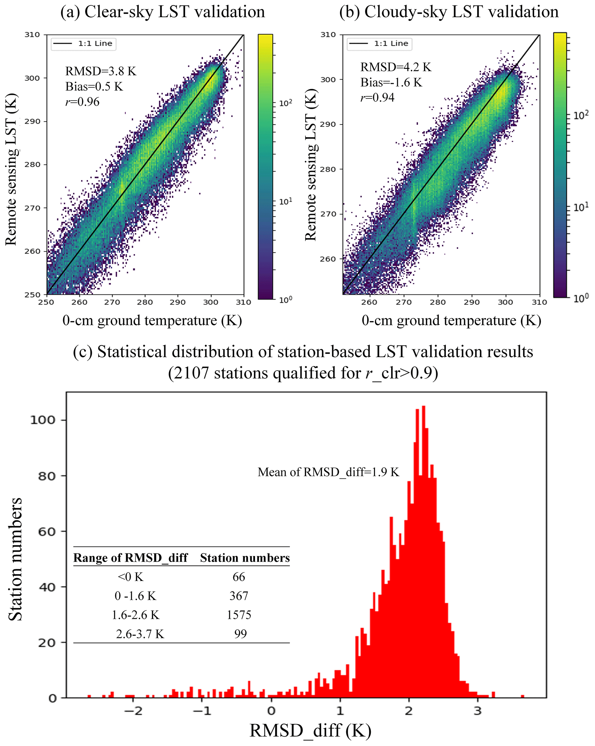
Figure 3 Validation results of the cloud gap-filled LST in China. (a) Density plot of thermal-infrared LST under clear-sky conditions compared to the 0 cm ground temperature measurements for all stations. (b) Same as (a) but for thermal-infrared LST under cloudy conditions. (c) Statistical distribution of difference between RMSD of clear-sky LST and RMSD of gap-filled LST under cloudy conditions with regard to different meteorological stations over the study region.

3.2 Evaluation of the final 1 km SSM product

The overall validation results of the finally downscaled 1 km SSM product against ground soil moisture data are shown in Fig. 4. Figure 4a shows that about 85 % (N: 1833) of the total 2154 stations (the remaining 263 stations are located in pixels with no effective PM observations and are thus removed) have obtained significantly positive downscaling gains (G_down>0.03). This hints that the 1 km SSM product can better capture the dynamic behaviors of local ground soil moisture data than the original 36 km PM NN-SM data, revealing higher spatial representativeness of the downscaled SSM data product over the country. According to Fig. 4b, the mean ubRMSD of all stations is about 0.054 vol vol⁻¹, while 90 % of those stations have a number lower than 0.088 vol vol⁻¹. In addition, we made another analysis concerning the possible influence of land cover types on SSM downscaling performance in Fig. 4c. The spatial information of land cover types was derived from the MODIS MCD12Q1 (https://doi.org/10.5067/MODIS/MCD12Q1.006; Friedl and Sulla-Menashe, 2019) International Geosphere Biosphere Programme (IGBP)-based land use image in 2019. For stations that experienced land use change throughout the years of the study period, the ubRMSD is only reported for data in the year 2019. Clearly, better accuracies are observed mainly in grassland, cropland, and bare soil surface, whilst relatively poorer performances (with averages of ubRMSD higher than 0.06 vol vol⁻¹) are seen in urban regions, (woody) savanna, and crop-to-natural-vegetation mosaic areas. Such a relative performance across land covers is logical because all the land cover types with their average ubRMSD higher than 0.06 vol vol⁻¹ are characterized by lower hydrologic homogeneity in terms of their definition, e.g., savanna, which is a mixture of grass and tall trees, and urban areas, which are composed of an impervious underlying surface.

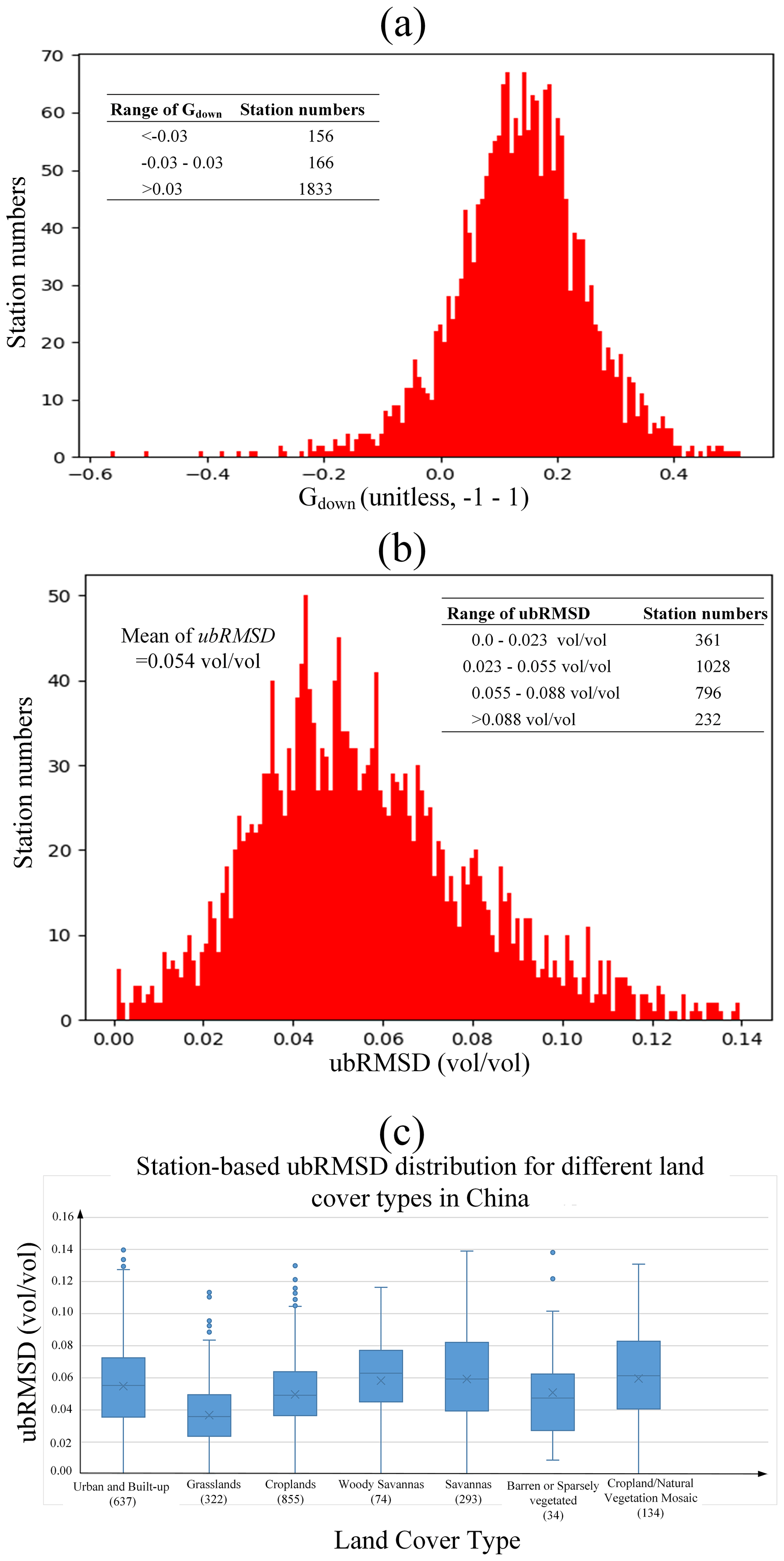
Figure 4 General validation results of the currently developed SSM product. (a) G_down distribution for different stations over China. (b) ubRMSD distribution for different stations over China. (c) ubRMSD statistics reported for different land covers. The numbers in the parentheses of the x axis labels represent the amount of meteorological stations corresponding to that specific land cover type.

In Fig. 5, we compared time series of regionally aggregated SSM from our developed 1 km SSM product to that from the SMAP 36 km descending SSM for each of the six different geographic–climate regions (as shown in Fig. 1) from 2016 to 2019. Via this effort, we mainly aim to reveal the consistency degree on reflecting soil moisture temporal dynamics at different geographical settings between the two SSM products. This also provides another view to evaluate the reliability of our developed product. Because the SMAP radiometer has a slightly longer revisit cycle (∼2–3 d) than AMSR-2, the time series data are also aggregated and averaged at the temporal dimension, with a displayed revisit cycle equal to 3 d. Overall, the time series data correlate well with each other for all six regions. The relatively lower RMSDs (<0.02 vol vol⁻¹) are found in regions with comparatively sparser vegetation cover including the NWA region, the QTP region, and the NCM region. For the other three dense vegetation regions, the performances of our developed product are slightly poorer. This is especially the case for the SCM region, with a lower r value of 0.84. The reason can be attributed to the enlarged difference in penetration depth into the soil layers between L-band (SMAP) and C-, X-, and K-band (AMSR-2) emissions under dense vegetation cover (Ulaby and Wilson, 1985).

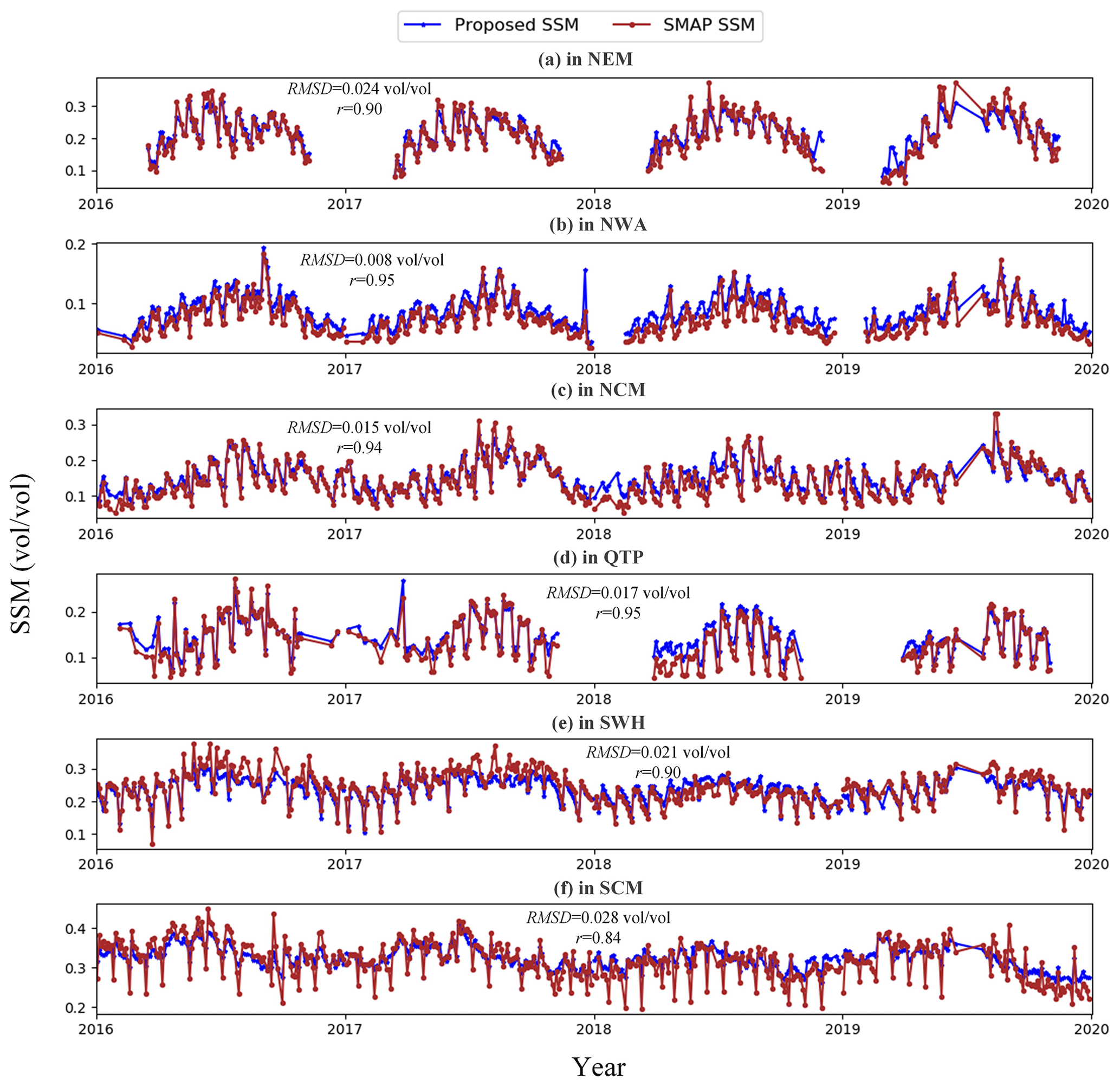
Figure 5 Time series of SSM aggregated at each of the six different geographic–climate regions (as shown in Fig. 1) in China for our developed 1 km product, as well as for the SMAP 36 km SSM dataset. The time series range is from 2016 to 2019 with a revisit cycle of 3 d.

In Fig. 6b we employed the downscaled SSM image on 29 May 2018 as an example to demonstrate the spatial features of the developed product. Meanwhile, we also show the map of SMAP–Sentinel combined SSM (SPL2SMAP_S_V3) obtained from 26 to 31 May 2018 in Fig. 6a as a contemporaneous comparison reference. Clearly, the SPL2SMAP_S_V3 map has a much lower coverage percentage over the study region compared with the map of the currently developed product on one single date even though the former was generated based on multi-date images. Both maps show similar spatial texture depicting the relatively dry climate in northwestern China compared with the humid climate in the middle-lower Yangtze River Plain. Nevertheless, there also exist cases where the details in texture differ prominently, like that in the far northeastern end of the country.

For the sake of further analysis on this point, results of the quantitative comparison as proposed in Sect. 2.1.3 and 2.1.4 are demonstrated in Fig. 6c–f. Figure 6c and d show the RMSD maps of the two respective products against SMAP radiometer-based SSM estimates at the 36 km pixel scale. For both products it is shown that compared with the lower averaged RMSD of 0.04 vol vol⁻¹ in the NWA region, the uncertainty can increase (shown in yellow) in the densely vegetated NEM and the SCM regions, with averaged RMSDs of 0.07–0.08 vol vol⁻¹. However, our developed product has noticeably lower RMSD (0.05 vol vol⁻¹) than the SPL2SMAP_S_V3 data (0.07–0.09 vol vol⁻¹) in the SWH and part of the QTP regions. Considering their relatively higher elevations, it may be roughly drawn that our downscaled SSM product is more reliable than that based on active–passive microwave combined datasets in areas with increased topographic effects. Figure 6e shows that the currently developed SSM product obtained a 0.078 vol vol⁻¹ ubRMSD and a correlation coefficient of 0.55 against the in situ soil moisture measurements. It converges more apparently to the 1:1 line when compared with validation result of the SPL2SMAP_S_V3 dataset in Fig. 6f. As with the area of China, therefore, the currently developed product is generally superior to the global SMAP–Sentinel combined SSM in terms of both coverage percentage and estimate accuracy.

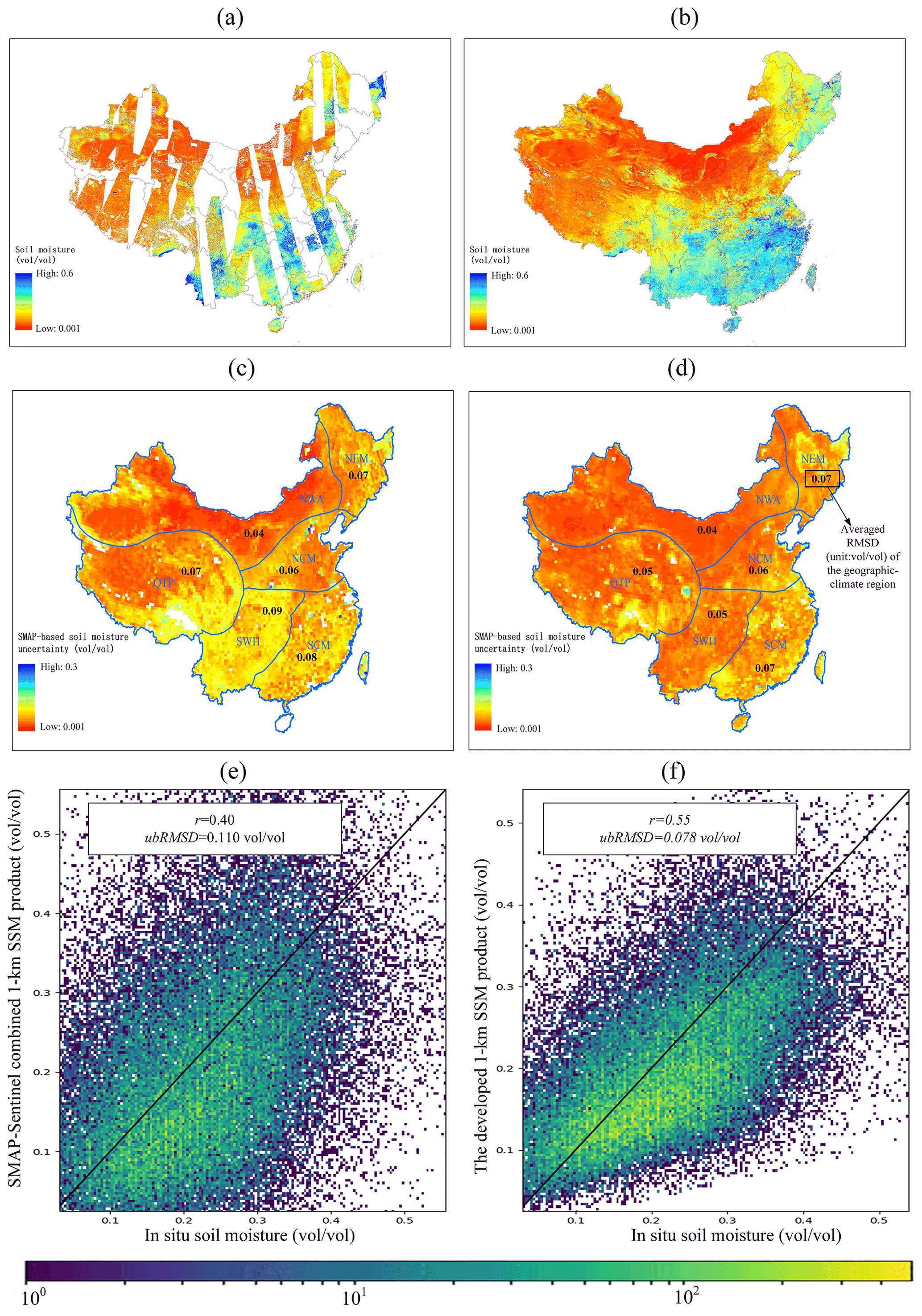
Figure 6 Comparison results between the currently developed 1 km SSM product and the SMAP–Sentinel combined 1 km SSM (SPL2SMAP_S_V3). (a) SPL2SMAP_S_V3 SSM images over the study area at about 06:00 LT synthesized by six continuous dates from 26 to 31 May 2018. (b) The SSM image at 01:30 LT of 29 May 2018 from the currently developed product. (c) Spatial uncertainty (RMSD) map of the SPL2SMAP_S_V3 product against SMAP radiometer-based SSM retrievals at the 36 km pixel scale over the study area for the years 2017, 2018, and 2019. (d) Same as (c) but for the validation of the currently developed SSM product. The black numbers in each of the geographic–climate regions indicate averaged uncertainty (RMSD, unit: vol vol⁻¹) of the region. (e) Validation results of the SPL2SMAP_S_V3 product against in situ soil moisture measurements over the study area for the years 2017, 2018, and 2019. The solid black line is the 1:1 line. (f) Same as (e) but for the validation of the currently developed SSM product.

In Fig. 7, we display the cumulative distribution frequency of coverage percentages of the downscaled SSM product and of the original PM NN-SM product for each season. It should be noted that in this statistical scheme, pixels identified as static water bodies by the MODIS MCD12Q1 land cover type product were not considered in the denominator of the coverage percentage. Moreover, the gap times between the respective on-orbit period of AMSR-E and of AMSR-2 (from October 2011 to June 2012, during which there are no effective observations from the PM NN-SM product) were also excluded. It is apparent that in Fig. 7b and c, almost all downscaled daily SSM images over the 16–17 years have achieved a coverage percentage higher than 85 %. In comparison, the majority of the PM NN-SM daily images have their coverage percentages below 80 % over the study region primarily due to the PM seam gaps particularly existing in low latitudes (see Sect. 2.2.2). In Fig. 7a and d, the percentages of effective pixels in both the PM and the downscaled SSM images are far lower than their counterparts in the other two subfigures. This is mainly ascribed to extreme meteorological conditions including snow, ice, and frozen soils that are typically persistent throughout most of these specified months in the northwestern regions of China. Such conditions can impede reliable estimates of SSM based on all satellite remote sensing techniques in the current time. The above inter-seasonal differences on data coverage are also reflected in Fig. 8 in another manner based on presenting the spatial distributions of number percentages of available dates in each 3-month period.

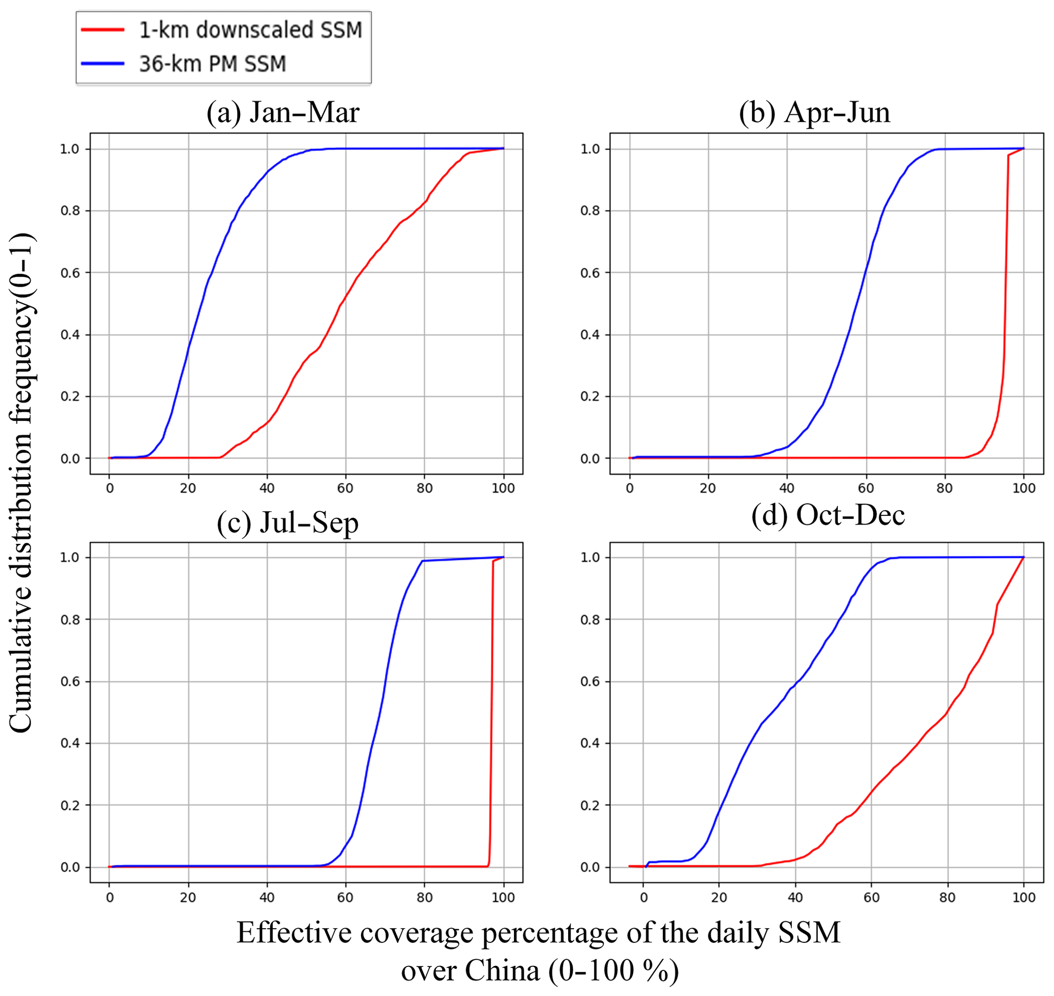
Figure 7 Cumulative distribution frequency of our proposed SSM product against the original 36 km SSM product for different seasons. The period between October 2011 and June 2012 is excluded in the current statistics.

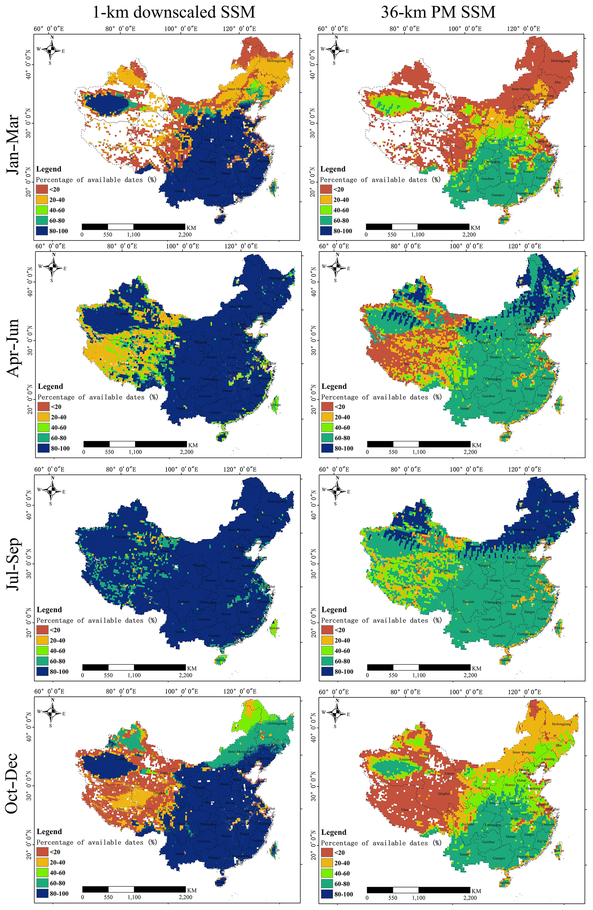
Figure 8 Spatial distributions of percentage of day numbers with available estimates for the currently developed 1 km SSM product and the original 36 km PM data during 2003–2019. The four different periods (i.e., January–March, April–June, July–September, October–December) of a year are treated respectively. The period between October 2011 and June 2012 is excluded.

The techniques behind the coverage improvement of the downscaled SSM (against PM and optical data inputs) can be categorized into two classes, i.e., cloud gap-filling of the input optical datasets (see Sect. 2.2.1), as well as the filling of downscaled SSM in PM seam gaps (see Sect. 2.2.2). Table 2 reports the specific validation results (using averages of ground measurements at all stations) of downscaled SSM in these coverage-improved conditions, relative to that generated without using any coverage improvement technique, in order to evaluate the propagated effect of such techniques on the final product. The very limited difference for ubRMSD values (0.053 versus 0.056 vol vol⁻¹) between cloudy and clear-sky conditions suggest that the 1 km SSM estimates from our final product are generally compatible between cloudy and clear-sky conditions. The downscaled SSM estimated for regions of PM seam gaps has a slightly worse (but still acceptable) accuracy, considering its ubRMSD of 0.059 vol vol⁻¹ compared to the 0.052 vol vol⁻¹ ubRMSD of the PM-observed 1 km pixels. In summary of Fig. 7 and Table 2, the currently developed product has achieved a substantially improved spatial coverage against the original remote sensing input datasets, whilst it successfully preserved the SSM downscaling accuracy of the observation-covered pixels at the same time.

Table 2 Comparisons between validation results for pixels under coverage-improved regions and for pixels under remote-sensing-observation-covered regions.

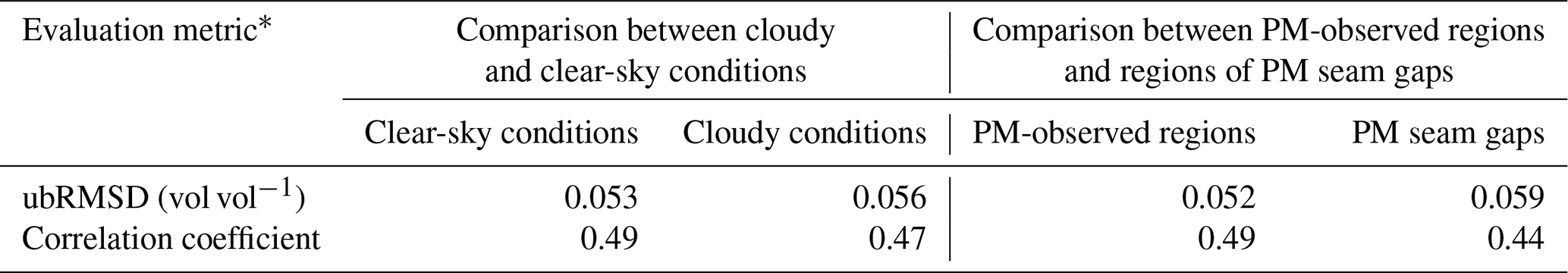
^∗ All evaluation metrics in this column indicate the average of all available stations.

4 Discussion

4.1 Uncertainty of SSM evaluation between satellite and ground scales

In this study, we made evaluations of remote sensing SSM products at different spatial resolutions using measurements from 2000+ stations provided by the national-level soil moisture observation network of China as the standard benchmark. Through the evaluations, a ubRMSD of 0.074 vol vol⁻¹ is reported for the original 36 km NN-SM SSM product (Fig. A1b). We notice that this result is considerably poorer if compared with another previous evaluation campaign targeted at the same product (Yao et al., 2021), which achieved a global RMSE (RMSD) of 0.029 vol vol⁻¹. However, this difference is not unexpected because the two campaigns were carried out in different regions of the world. Also, that particular study (Yao et al., 2021) was conducted based on completely different ground soil moisture observations provided by the International Soil Moisture Network (ISMN) (Dorigo et al., 2021). Compared to the observation network employed in this study, the observation sites of ISMN are more intensively distributed as an “integrated soil moisture station” so as to provide spatially averaged soil moisture within a grid of tens of kilometers. In this regard, we admit that the ISMN is generally more professional in evaluating satellite PM-based SSM retrievals at a coarser resolution. But on the other hand, only a few (≤4) of such “integrated stations” have been set up sporadically within China, making the ISMN data much less representative of our study region compared with the national-level soil moisture network of China exploited by our current study.

Although the higher RMSD of the national-level soil moisture network of China may indicate larger measurement uncertainty than the ISMN, the negative influence that might be imposed on our study purpose should be inconsequential. This is because we focus more on the relative validation performance of different SSM products rather than on the absolute value of any evaluation metric including ubRMSD and the correlation coefficient calculated against ground measurements. Specifically, the 1 km downscaled SSM obtained an average ubRMSD of about 0.054 vol vol⁻¹ among different stations according to Fig. 4b. Moreover, the result of the evaluation in Fig. 6d based on combination of multi-station ground measurements shows a global ubRMSD of 0.078 vol vol⁻¹ for this product. Overall, the above-mentioned results can be identified as at least comparable to the global (multi-station-based) ubRMSD of 0.074 vol vol⁻¹ of the original NN-SM data as they are evaluated against the same benchmark. Therefore, the conclusion is safely drawn that the currently developed product preserves the retrieval accuracy of the coarse-resolution NN-SM data whilst improving the spatial representativeness of the latter product substantially according to the mostly positive G_down values in Fig. 4a.

Moreover, one may also argue that the r value of 0.55 for the currently developed product in Fig. 6d is not sufficiently high compared with several previous studies (Wei et al., 2019; Sabaghy et al., 2020) obtaining r values above 0.7 for the temporal analysis of satellite remote sensing soil moisture. However, we should note that these previous studies have conducted analyses respectively at the temporal and the spatial dimensions. Based on their results, the spatial analysis typically derived lower r values (<0.4) compared to that at the temporal dimension. This is probably because the heterogeneity degree of remote sensing pixels can vary significantly across different sites. Since the evaluation in Fig. 5d was deployed at the “spatiotemporal” integrated dimensions, such an r value is expected. This is also close to the global r value of 0.6 for the validation of the coarse-resolution NN-SM product as reported in Yao et al. (2021).

4.2 Uncertainty of cloud gap-filling and validations of LST

As mentioned in Sect. 2.2.1, LST gap-filled based on the STDF method was used alone as one of the main input datasets for SSM downscaling under cloudy weather. Although such LST inputs contain clear-sky bias from the real cloudy conditions, it performs better in driving the SSM downscaling model compared with its bias-adjusted counterpart (see Appendix B for details). The reason may be linked to one of the basic theories behind our SSM downscaling methodology, i.e., the UTFS theory (Carlson et al., 1994). In the UTFS theory, clear-sky LST is employed to implicitly quantify the surface soil wetness degree as it correlates with the dynamics of soil evaporative efficiency and soil thermal inertia when vegetation cover density is fixed. Under cloudy conditions, however, the satellite observed LST is subjected not only to surface soil property but also to that related to cloud insulation effect from solar incoming radiation and ground longwave outgoing radiation. As a result, the actual relationship between SSM and cloudy LST could be much more complicated than the one that has been described by the UTFS-based SSM downscaling model (i.e., Eq. 2). In comparison, LST generated by the STDF alone for assumed clear-sky conditions, free from the interference of cloud, would be a comparatively more competent input variable for driving the UTFS-based SSM downscaling model under non-rainy clouds. This is especially the case for thin and short-period clouds with marginal direct feedbacks on surface soil wetness.

However, we admit that the STDF-filled LST under rainy clouds is also not suitable for our study purpose. This may explain the slightly higher RMSD for SSM under cloudy conditions based on STDF-filled LST (0.056 vol vol⁻¹) compared to that under real clear-sky conditions (0.053 vol vol⁻¹), as shown in Table 2. In reality, the actual negative influence of cloud on the final SSM product may be even more serious than indicated from the above RMSD difference (i.e., 0.056–0.053 = 0.003 vol vol⁻¹) due to the portion of clear/cloudy-weather-mixed spatial windows during the fitting process of the downscaling model. In these windows, uncertainty in cloud gap-filled LST may affect accuracy of the fitted model coefficients and thus deteriorate the final SSM estimates in clear-sky pixels within the same window. Consequently, the above RMSD difference has been more or less underestimated. Despite all of the above, in our study area of China we regard the STDF-filled LST as a more optimal proxy of heat flux for estimating SSM under cloudy conditions, compared to the bias-adjusted LST. On the other hand, future efforts are encouraged to further clarify the mechanical relationships between STDF-filled and/or bias-adjusted LST and soil wetness degree under cloudy conditions.

Different from a number of previous studies (Jiménez et al., 2017; Dowling et al., 2021; Yang et al., 2019) validating satellite thermal-infrared-based LST based on longwave radiation observations made at footprint-level observation stations (e.g., flux towers), our study has used 0 cm top ground temperatures as the primary benchmark for this validation campaign instead. Similar to that for SSM validation, the most crucial motivation driving such an experimental design is the significantly intensive distribution of the meteorological stations compared to the very limited number of active and effective flux towers available in China. It is noted that these measurement devices at all of the meteorological stations are required to have been instrumented under open environmental conditions with a relatively lower fraction of tall trees and water bodies in order to conduct efficient monitoring at the physics of near-surface air. This can also be reflected in Fig. 4c, which reveals no stations built within forest cover. Moreover, as we only focus on the midnight scenario when the states of all land observations are “most stable” during one diurnal cycle, uncertainties due to the possible temperature inconsistency between bare ground surfaces and high tree surfaces, as well as due to the temporal mismatch (from about 01:30 to 02:00 LT), should have marginal effects on our results. We have carried out an extra test that can confirm this discussion, with the detailed procedures described in Appendix C.

4.3 Major novelty, unique profit, and future prospect of the developed product

Compared with the widely known active–passive microwave combined SSM product (e.g., the SPL2SMAP_S_V3) and other PM–optical-data combined counterparts which were also published recently but at the monthly scale (Meng et al., 2021), the major novelty of the currently developed product mainly lies in the fact that it has achieved progress in all of the three crucial dimensions of satellite remote sensing, including the temporal revisit cycle (daily), the spatial resolution (1 km), and the quasi-complete coverage under all-weather conditions. To our knowledge, this has rarely been achieved by previously developed satellite soil moisture products at regional scales. For the realization of the above-mentioned progress, we have fused the SSM downscaling framework with other techniques including cloud gap-filling of thermal-infrared LST, MWS-based temporal filtering of vegetation indices, and reconstructions of seams between neighboring PM swaths in low latitudes. The final SSM estimates under cloudy conditions and intersected with the PM seam gaps were specially validated against the rest of the estimates under clear-sky conditions and in the regions covered by PM observations, respectively (Table 2). The comparable performances among all treatment groups herein confirm that the accuracy of the product is stable and consistent among all-weather conditions.

With improvement achieved at the three dimensions, unique profit of the currently developed product can be taken by subsequent studies and various industrial applications. For example, the capability of this product can be investigated on capturing the short-term anomaly of local hydrological signals as well as improved monitoring on drought disasters, which used to be investigated mainly at a coarser resolution by PM SSM (Scaini et al., 2015; Champagne et al., 2011; Albergel et al., 2012). For another, taking advantage of its all-weather daily time series, the product can be utilized together with precipitation data to isolate and quantify the anthropic influence on regional water resources from the natural hydrological dynamics. Examples of such anthropic signals include agricultural irrigation activities, as well as finer-scale information on agricultural crops which was previously interpreted based on PM-driven techniques (Song et al., 2018). In addition, we should realize the important role of soil moisture as a constraint for the accurate estimation of surface evapotranspiration and runoff (Zhang et al., 2020, 2019). Therefore, the profit of this product can be further enhanced if coupled with land–atmosphere-coupled models to produce new insights into water-cycle processes of the earth surface at a finer spatiotemporal scale.

There are still some limitations on our current product to be further improved. First, there may exist the “mosaic effect” at the original PM (36 km) pixel edge. As mentioned in Sect. 2.2.2, we have used a parameter of “spatial square window (w_s)” in Eq. (3) to minimize this negative effect. However, it is still difficult to utterly avoid such a negative effect. This is a challenge for all existing SSM downscaling methods (Molero et al., 2016; Stefan et al., 2020; Peng et al., 2016), especially considering the large spatial scale of our study and all uncertainties discussed in Sects. 4.1 and 4.2. Moreover, other negative influences can be imposed by potential imperfections identified from the original PM product, e.g., from PM SSM retrievals in the QTP region with complicated topography, melt snow, or partially frozen soils that cannot be completely screened out by the original product flag in winter. For these extreme conditions, the accuracy of the downscaled SSM may need further validation campaigns like field surveys and experiments, based on which the data quality flag can be better built for the product's future version.

The methodological framework proposed in this paper has the prospect to be universally applied in other regions of the world to serve for better monitoring of the global surface wetness in the following studies. If applied at continental and global scales, however, the current process for gap-filling of PM seams may require further attention and improvement. In this study, SSM in regions intersected with PM seam gaps was estimated using TB observations from PM swaths at neighboring dates (see Eq. 5). Although the errors in the PM seam gaps over China as reported by Table 2 are only slightly larger compared to the PM-covered regions, they cannot be ignorable completely and may leave extra concern on the universality of this technique, especially in the low-latitudinal tropical regions where the effect of PM seam gaps is more apparent than in our study area. Moreover, another imperfection of this data product lies in the gap period between AMSR-E and AMSR-2. Considering the different systematic error patterns of various PM SSM products, we did not generate downscaled SSM based on other PM products (e.g., the SMOS SSM product) during this period but just left the period as null values. We suggest a more rigorous and universal inter-calibration framework on different PM SSM products to be developed in the future for a long-term, consistent 1 km downscaled SSM dataset.

5 Data availability

The published SSM dataset is available under the Creative Commons Attribution 4.0 International License at the following link: https://doi.org/10.11888/Hydro.tpdc.271762 (Song and Zhang, 2021b). This dataset covers all of China's terrestrial area at a daily revisit frequency (about 01:30 LT) and a 1 km spatial resolution from January 2003 to October 2011 and from July 2012 to December 2019.

6 Conclusions

This paper describes the main technical procedures of a recently developed remote sensing surface soil moisture (SSM) product over China covering the most recent 10 years and more. Based on a combination of passive microwave SSM downscaling theory and other related remote sensing techniques, the product achieves multi-dimensional distinctive features including 1 km resolution, daily revisit cycle, and quasi-complete all-weather coverage. These were rarely satisfied completely by other existing remote sensing SSM products at regional scales. Validations were conducted against measurements from 2000+ automatic soil moisture observation stations over China. Overall, an average ubRMSD of 0.054 vol vol⁻¹ across different stations is reported for the currently developed product. The mostly positive G_down values show this product has significantly improved spatial representativeness against the 36 km PM SSM data (a major source for downscaling). Meanwhile, it generally preserves the retrieval accuracy of the 36 km data product. Moreover, additional validation results show that the currently developed product surpasses the widely used SMAP–Sentinel combined global 1 km SSM product, with a correlation coefficient of 0.55 achieved against that of 0.40 for the latter product. At the regional scale, time series patterns of our developed data product are highly correlated with those of the widely recognized SMAP radiometer-based SSM for all geographic settings. The methodological framework for product generation shows promise in being applied at the continental and global scales in the future, and the product has the potential to benefit various research and industrial fields related to hydrological processes and water resource management.

Appendix A: Evaluation of different PM SSM products

We have made evaluations of the various AMSR-based SSM products (as shown in Table 1) covering the most recent 10 years or longer, based on our soil moisture observation network all over China. The SMAP radiometer-based SSM dataset, as described in Sect. 2.1.4, was also evaluated as a reference. The evaluation period covers the years of 2017, 2018, and 2019. All AMSR-based 25 km grids were re-set to the SMAP 36 km grid system using the nearest resampling method. Only grids that contain as many as or more than four soil moisture measurement stations were employed, in which the grid-based PM SSM estimate was compared with the average measurements from all interior stations. Finally, 53 grids were selected, as shown by the green color in Fig. A1g. For AMSR-based products, only the midnight descending datasets were evaluated, whilst for the SMAP product, our evaluation only focused on its descending mode in the early morning.

As shown in Fig. A1a–f, the selected SSM product in the current study, i.e., the NN-SM product, has an unbiased RMSD of 0.074 vol vol⁻¹ and a correlation coefficient of 0.49. This obviously outperforms the other three traditional AMSR-based SSM products (i.e., JAXA-AMSR, LPRM-AMSR, and UMT-AMSR products) and is only inferior to the SMAP SSM retrievals, whilst the later only covers the latest period since 2015. As far as CCI data are concerned, it has a similar performance against the selected NN-SM in general. Nevertheless, the region marked by the red circle in Fig. A1c indicates that CCI estimates have a considerably larger proportion of overestimated anomalies. But overall, the primary reason that we have abandoned CCI but selected NN-SM is because the latter can provide a higher coverage fraction of valid pixels in our study region, as has been stated in Sect. 2.1.1.

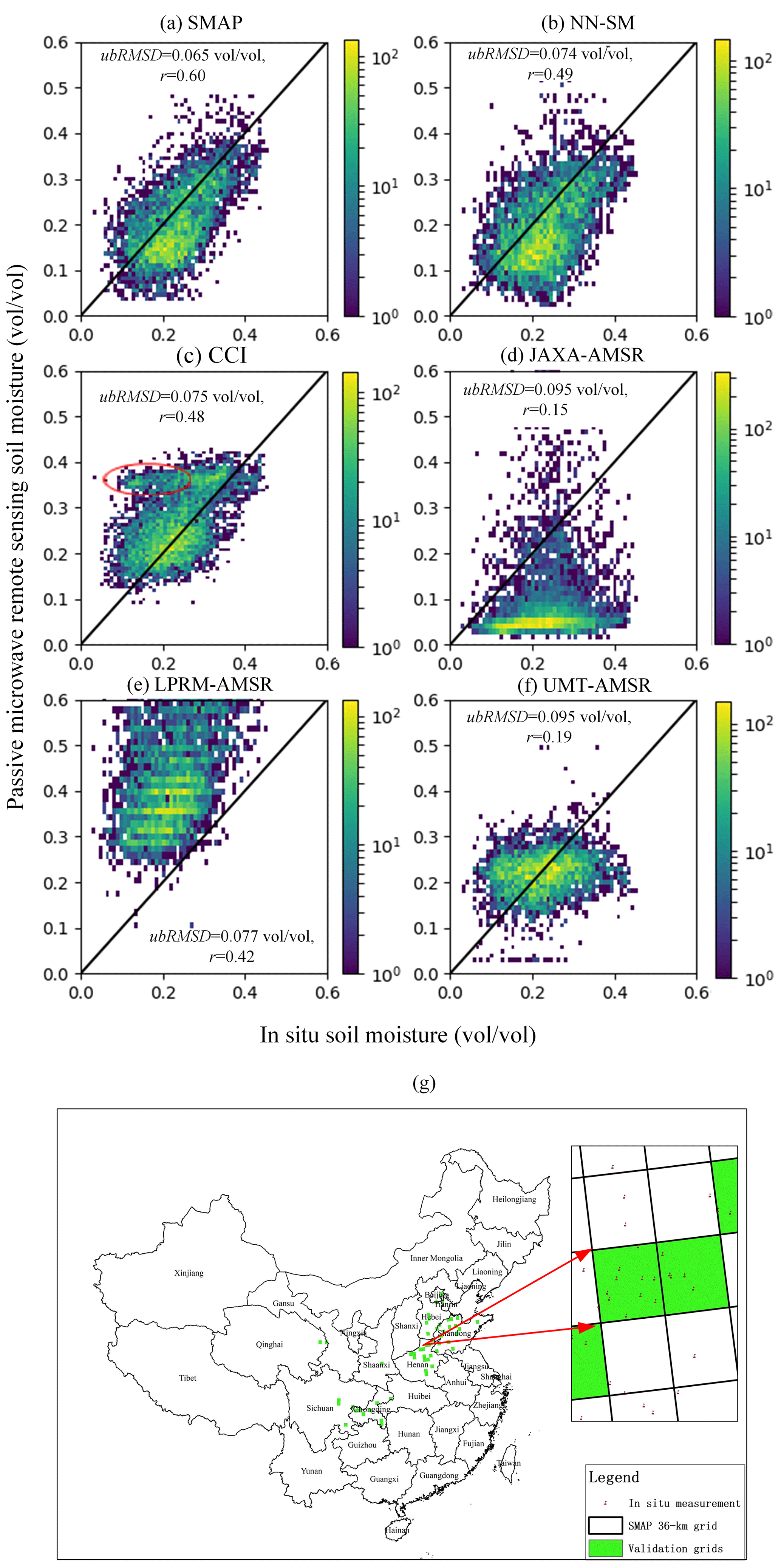
Figure A1 (a–f) Comparison of different PM SSM products (as reported in Table 1) against the in situ SSM measurements in China. (g) Locations of the 36 km EASE-Grid projection-based pixels used for this comparison campaign.

Appendix B: Evaluation of the influence of bias adjustment for reconstructed “clear-sky” LST under cloudy conditions

In Sect. 2.2.2, we have emphasized that the gap-filled LST for cloudy pixels reflects the theoretical surface temperature of that pixel under hypothetical clear-sky conditions. As this cloud gap-filled LST would suffer from a possible bias against the real surface temperature under cloudy conditions (Dowling et al., 2021), we made an additional experiment regarding further improvement of this cloud gap-filled LST. The follow-up step for bias adjustment of this hypothetical clear-sky LST (but actually under cloudy conditions), as expounded in Sect. 4.2 of Dowling et al. (2021), was conducted herein using remote sensing and in situ LST data over China but only in 2018. We illustrate the validation results for bias-adjusted and non-bias-adjusted LST under cloudy conditions in Fig. B1b and c, respectively. Similar to Fig. 3, validation results for clear-sky LST of that year are also displayed (Fig. B1a) for comparison. The results generally show that the follow-up step is effective in reducing the bias of the originally gap-filled clear-sky LST under cloudy conditions (from −1.7 to 0.4 K).

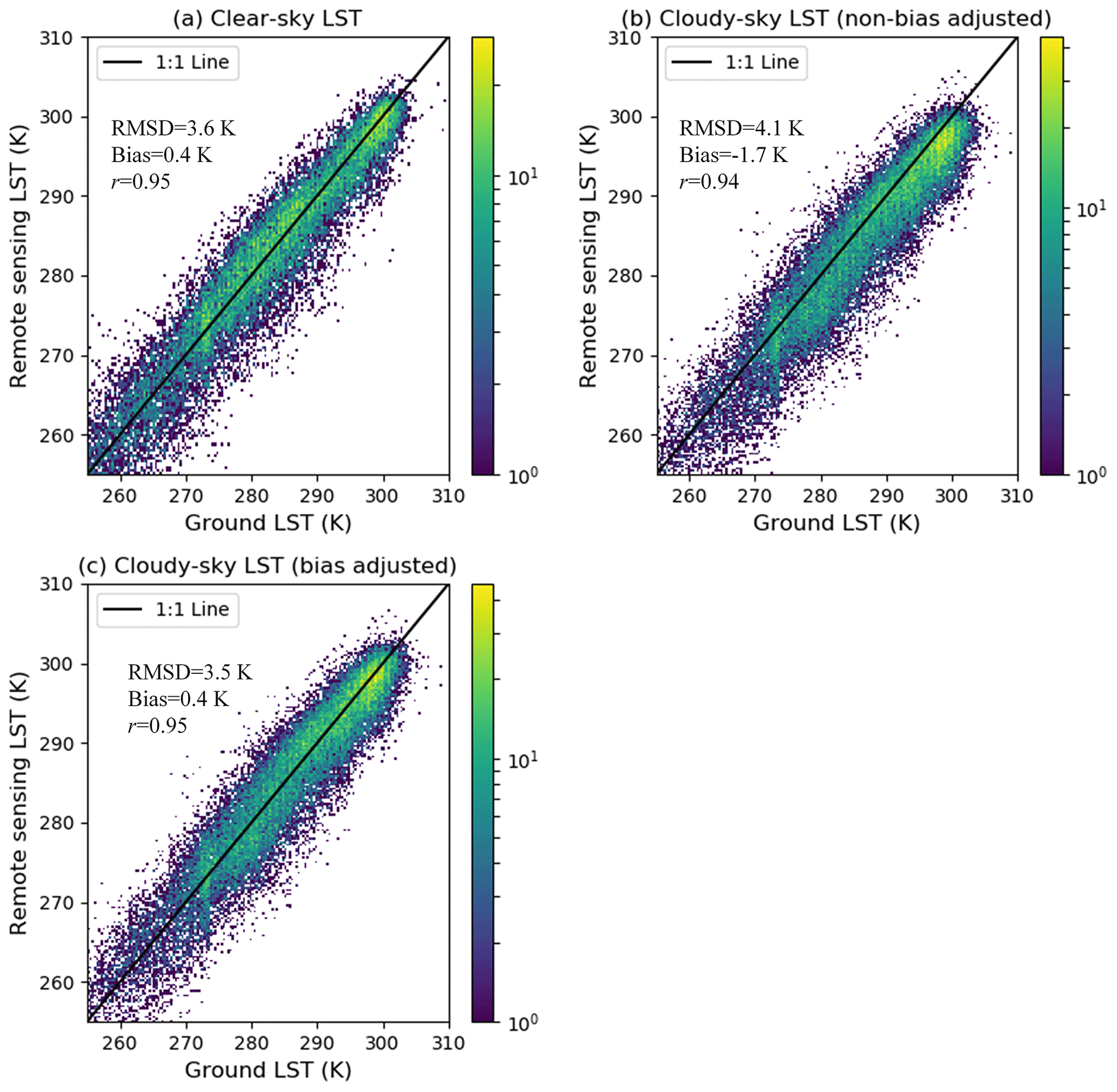
Figure B1 Validation of the clear-sky LST (a), reconstructed LST under cloudy conditions but with no passive-microwave-based bias adjustment (b), and the reconstructed LST under cloudy conditions with passive-microwave-based bias adjustment (c) based on the 0 cm ground temperature measurements at meteorological stations.

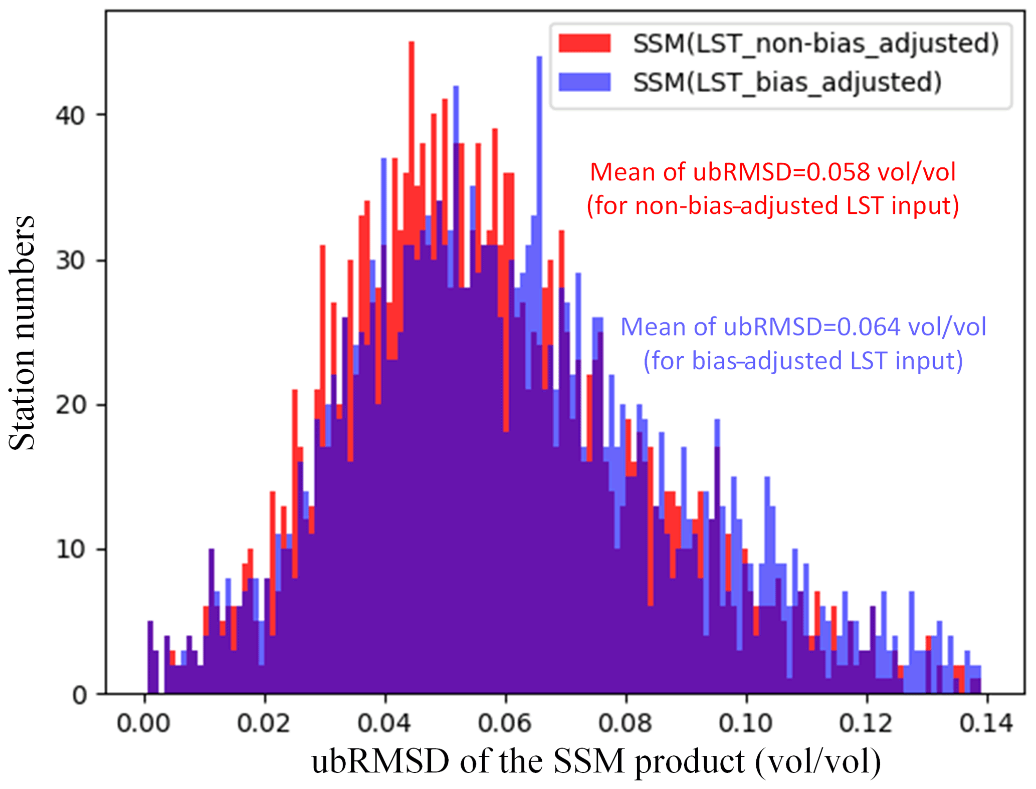
Figure B2 The statistical distribution of ubRMSD at different stations for SSM estimates driven by two respective kinds of cloudy LST inputs.

In the subsequent step, we substituted the original non-bias-adjusted LST under cloudy conditions with its bias-adjusted counterpart and used the latter as the input for SSM downscaling. The general validation results of the downscaled SSM are illustrated in Fig. B2 (similar to that presented in Fig. 4a and b). Contrary to the above-analyzed Fig. B1, the bias-adjusted cloudy LST with better gap-filling accuracies, however, obtained inferior performance in SSM downscaling. This final validation result, to some degree, confirms our assumption in Sect. 2.2.2 that the reconstructed cloudy LST but for the hypothesized clear-sky conditions is the better proxy of surface moisture dynamics. But overall, as all LST estimates discussed herein are for the midnight scenario (when the energy interaction between atmosphere and land surface is relatively weak), the RMSD difference for different weather conditions in Fig. B1 is expectedly marginal. As a consequence, the difference in ubRMSD of SSM in Fig. B2 can hardly be identified as “very significant”. Therefore, we encourage further tests on this conclusion in specific future studies to confirm its universality, especially for situations of the “morning to noon” time window.

Appendix C: Uncertainty test between 0 cm ground temperature observations and flux-tower-derived thermal-infrared LST

Figure C1 (a) Comparison of LST between 01:00–01:30 and 01:30–02:00 LT for the four selected flux towers. (b) Comparison of flux-tower-derived LST averaged for 01:00–02:00 LT at the four towers and corresponding nighttime 0 cm ground temperature at proximal meteorological stations. The inset map shows the location of the four flux towers. (c) Monthly NDVI time series for 1 km pixels containing each of the four flux towers.

We herein utilized four flux towers to calculate their footprint-level (about 500–1000 m) thermal-infrared LST based on longwave radiation measurements, plus broad-band emissivity data derived from the MODIS MYD21A1 product (MYD21A1N.V061). The four towers are all characterized by moderate or low vegetation (grassland) and are dispersedly located at different eco-regions of China, namely the towers of Changling, Huailai, Yakou, and Naqu (see the inset map in Fig. C1b). Data from Changling are derived from the FLUXNET community (FLUXNET2015 Dataset – FLUXNET; Pastorello et al., 2020) in 2010. Data from the other three towers are derived from the National Tibetan Plateau Data Center, with data DOIs of https://doi.org/10.11888/Meteoro.tpdc.271094 (Liu et al., 2021) for Huailai in 2018, https://doi.org/10.11888/Meteoro.tpdc.270781 (Liu et al., 2019) for Yakou in 2018, and https://doi.org/10.11888/Meteoro.tpdc.270910 (Ma, 2020) for Naqu in 2016. These data have been preprocessed by their providers to record the dynamics of those variables at a half-hour interval. The algorithm for calculating LST based on flux-tower-derived longwave radiation is inherited from Wang and Liang (2009). We first compared the flux-tower-derived nighttime LST estimates between 01:00–01:30 and 01:30–02:00 LT. As shown by Fig. C1a, the very slight RMSD of 0.72 K suggests that LST is generally stable between 01:00 and 02:00 LT at night. In Fig. C1b, we also found marginal bias and RMSD within 1 K between average flux-tower-derived LST of 01:00–02:00 LT and the corresponding 0 cm ground temperature at close meteorological sites (within 1 km and at 02:00 LT).

In Fig. C1c we demonstrate time series for monthly average NDVI (derived as in Sect. 2.2.1) at the 1 km pixels containing each of the four sites from 2003–2019. Clearly, there are very rare cases with NDVI values exceeding 0.5, corroborating the “open environmental conditions” met by the meteorological stations. In view of the above, it is feasible for our study to have used the 0 cm ground temperature at pixels of such moderate to low vegetation cover as the evaluation benchmark of the satellite-derived thermal-infrared LST.