the Creative Commons Attribution 4.0 License.
the Creative Commons Attribution 4.0 License.
 | 13 May 2022
A global long-term (1981–2019) daily land surface radiation budget product from AVHRR satellite data using a residual convolutional neural network
Jianglei Xu
Bo Jiang
The surface radiation budget, also known as all-wave net radiation (Rn), is a key parameter for various land surface processes including hydrological, ecological, agricultural, and biogeochemical processes. Satellite data can be effectively used to estimate Rn, but existing satellite products have coarse spatial resolutions and limited temporal coverage. In this study, a point-surface matching estimation (PSME) method is proposed to estimate surface Rn using a residual convolutional neural network (RCNN) integrating spatially adjacent information to improve the accuracy of retrievals. A global high-resolution (0.05∘), long-term (1981–2019), and daily mean Rn product was subsequently generated from Advanced Very High Resolution Radiometer (AVHRR) data. Specifically, the RCNN was employed to establish a nonlinear relationship between globally distributed ground measurements from 522 sites and AVHRR top-of-atmosphere (TOA) observations. Extended triplet collocation (ETC) technology was applied to address the spatial-scale mismatch issue resulting from the low spatial support of ground measurements within the AVHRR footprint by selecting reliable sites for model training. The overall independent validation results show that the generated AVHRR Rn product is highly accurate, with R2, root-mean-square error (RMSE), and bias of 0.84, 26.77 W m−2 (31.54 %), and 1.16 W m−2 (1.37 %), respectively. Inter-comparisons with three other Rn products, i.e., the 5 km Global Land Surface Satellite (GLASS); the 1∘ Clouds and the Earth's Radiant Energy System (CERES); and the 0.5∘ × 0.625∘ Modern-Era Retrospective analysis for Research and Applications, Version 2 (MERRA-2), illustrate that our AVHRR Rn retrievals have the best accuracy under most of the considered surface and atmospheric conditions, especially thick-cloud or hazy conditions. However, the performance of the model needs to be further improved for the snow/ice cover surface. The spatiotemporal analyses of these four Rn datasets indicate that the AVHRR Rn product reasonably replicates the spatial pattern and temporal evolution trends of Rn observations. The long-term record (1981–2019) of the AVHRR Rn product shows its value in climate change studies. This dataset is freely available at https://doi.org/10.5281/zenodo.5546316 for 1981–2019 (Xu et al., 2021).
- Article
(13132 KB) - Full-text XML
-
Supplement
(1333 KB) - BibTeX
- EndNote


Net radiation (Rn), which characterizes the surface radiation budget, is the difference between downward and upward radiation across the shortwave (0.3–3.0 µm) and longwave (3.0–100 µm) spectra. The surface radiation budget links the atmospheric climate system to the land surface. Rn is thus a critical variable for studying Earth–atmosphere interactions, including meteorological, hydrological, and biological processes, and is also responsible for the redistribution of surface available energy (Sellers et al., 1997). Accurate characterization and quantification of spatial–temporal variations in surface Rn are essential for both scientific and industrial applications, such as hydrological modeling and water resource management (Hao et al., 2019). However, because the spatial and temporal dynamics of surface Rn are affected by multiple surface features (e.g., albedo, emissivity, and land surface temperature) and atmospheric parameters (e.g., clouds, aerosols, ozone, and water vapor) (Wang et al., 2015b), existing surface Rn data suffer from large uncertainties (Jia et al., 2016, 2018; Jiang et al., 2018; Yang and Cheng, 2020). Therefore, there is an urgent need for a long-term, high-resolution surface Rn dataset to more properly understand the spatial pattern and temporal dynamics of Rn (i.e., seasonal and inter-annual variability).
Traditionally, historical Rn and surface radiative components have been measured at ground meteorological stations. These ground-based measurements are widely used to study spatiotemporal variations in regional surface radiation and to evaluate gridded products (Jia et al., 2018; Zhang et al., 2020, 2015). Nevertheless, the high cost of maintaining radiometers means that stations are sparsely distributed, severely hindering our ability to study and understand the spatiotemporal variability in surface Rn at the global scale.
Alternatively, reanalysis products provide long-term global surface Rn information (Zhang et al., 2016). The greatest advantage of reanalysis products is their global coverage over a long-term period; however, the large uncertainty and coarse spatial resolution of reanalysis products hinder their applications at a regional spatial scale (Jia et al., 2018; Zhang et al., 2016; Zhang et al., 2020).
Retrieving Rn from satellite data is another effective method (Liang et al., 2010, 2019). Currently, satellite-based Rn retrieval methods can be broadly divided into two categories, physical methods based on radiative transfer (RT) and empirical statistical methods. RT-based physical methods are more applicable to a larger spatiotemporal extent because they consider the physical processes of solar radiation from the top of the atmosphere to the Earth's surface (Tang et al., 2019). The look-up-table (LUT) and parameterization methods are two typical physical schemes that are widely used to estimate surface radiation from satellite data. To address the low computational efficiency of the radiative transfer model (RTM), the LUT method was proposed to estimate the surface radiation from satellite top-of-atmosphere (TOA) observations, which combines the advantages of RTM-based simulations and statistical methods (Wang et al., 2015b, a; D. Wang et al., 2020; Cheng and Liang, 2016; Cheng et al., 2017; Huang et al., 2011). This approach relies on several theoretical assumptions in the RTM simulation process, such as water vapor amounts, aerosol types, plane-parallel homogeneous clouds, horizontal homogeneity, and directional properties of the surface (Jiang et al., 2019b), which results in errors in the final radiation estimates (Hao et al., 2018; Cheng et al., 2017; Jiao et al., 2015). The parameterization scheme is another typical physical method that uses various surface and atmospheric parameter data to calculate surface radiation based on simplified RT (Huang et al., 2020; Qin et al., 2012). However, in the calculation of parameterized formulas, errors from each input variable accumulate in the final calculated surface radiation.
Conversely, differently from physical methods, empirical statistical methods typically account for spatial–temporal variations in Rn by establishing statistical relationships between satellite measures or sensed variables, including surface and atmospheric variables or TOA observations, and surface radiation measurements (Tang et al., 2017; Huang et al., 2020; Jiang et al., 2015; Bisht and Bras, 2010; Bisht et al., 2005) using linear or nonlinear models. Machine learning (ML) has played an important role in the development of empirical statistical methods owing to its strong nonlinear fitting ability (Jiang et al., 2014, 2016; Chen et al., 2020; Xu et al., 2020). Although statistical methods incorporate very little physical knowledge and have limited ability to expand their coverage, they are still widely employed owing to their low computational cost and easy implementation.
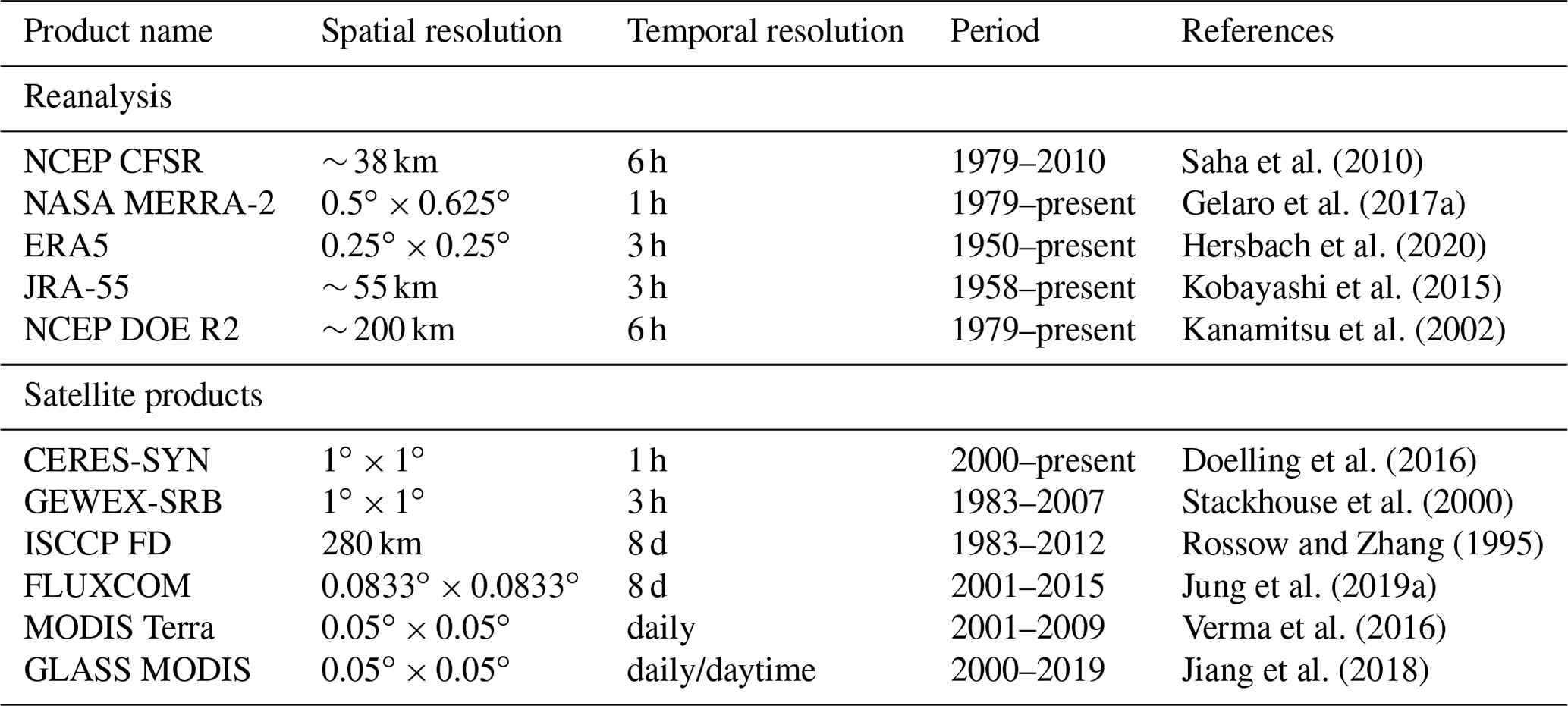
Several well-known global Rn datasets have been generated from satellite data (Table 1), such as the Global Energy and Water Cycle Experiment surface radiation budget (GEWEX-SRB) (Pinker and Laszlo, 1992), the Clouds and the Earth's Radiant Energy System (CERES) (Loeb et al., 2018), and the International Satellite Cloud Climatology Project (ISCCP) (Zhang et al., 2004). Although these products have been widely used in various fields, their coarse spatial resolution (≥ 100 km) cannot meet the requirements of high-resolution Rn data. A high-resolution (5 km) global Rn product was recently released (Jiang et al., 2018) from the Global Land Surface Satellite (GLASS) product suite (Liang et al., 2020). The GLASS Rn product, which has been available since 2000, was produced from the Moderate Resolution Imaging Spectroradiometer (MODIS) data and reanalysis products. The FLUXCOM initiative recently published a gridded product of surface Rn using multiple ML methods to merge energy flux measurements with remote sensing and meteorological data to estimate Rn retrievals, but the product only provides available data on areas covered by vegetation and the dataset only spans 15 years (Jung et al., 2019b). A long-term, high-resolution, and accurate surface Rn dataset is, therefore, still urgently needed to help more clearly understand the long-term spatiotemporal variation in global surface Rn.
In this study, deep learning ML methods were explored to produce a long-term, high-resolution surface Rn dataset from Advanced Very High Resolution Radiometer (AVHRR) data. Reviewing recent studies on surface Rn estimation using ML methods, many significant advancements have been made (Jiang et al., 2014; Letu et al., 2020; Wei et al., 2019; Wang et al., 2019); however, clear deviations still exist between satellite-derived estimations and ground-based measurements. Apart from the performance of the ML method itself, many of these discrepancies are attributed to two aspects: first, the spatial representation mismatch between satellite data and ground-based measurements and, second, the neglect of spatially adjacent effects on surface radiation estimation.
The spatial-scale mismatch between surface radiation for domain averages and ground point measurements with insufficient spatial representativeness (Jiang et al., 2019b; Barker and Li, 1997) has attracted attention for a long time in the development of ML (Yuan et al., 2020a) and in the evaluation of gridded products (Huang et al., 2016; Yang, 2020; Román et al., 2009). However, many current studies still use matched point-surface sample datasets to train ML models regardless of the difference in spatial representativeness of matched point-surface data. The triple collocation (TC) technique (Stoffelen, 1998) was considered an appropriate upscaling approach for the impact of random measurement error on ground-based measurements in comparison to other complicated upscaling methods (e.g., the time stability approach and the block kriging algorithm; Crow et al., 2012; Yuan et al., 2020a). Furthermore, an extended triple collocation (ETC) method was proposed by McColl et al. (2014) and then applied to the validation activities of the Soil Moisture Active Passive (SMAP) level-2 surface soil moisture (SSM) product (Chen et al., 2017) and satellite surface albedo products (Wu et al., 2019). Therefore, the ETC technology is employed to limit the effect of upscaling errors in ground measurements on the final surface Rn estimates at the satellite footprint scale.
Spatially adjacent effects should also be considered in the development of ML methods. With an increase in spatial resolution, horizontal inhomogeneities in the atmosphere have become increasingly important and reduce accuracy of surface radiation retrievals at higher spatial resolutions, especially in conjunction with high solar and viewing angles (Wyser et al., 2002); the correlation between satellite TOA observations and surface radiation measurements weakens, and surface radiation cannot be accessed directly from satellite TOA data for individual pixels. Convolutional neural networks (CNNs) were initially designed to perform image recognition tasks; they can be readily used to extract various high-level, hierarchical, and abstract spatial pattern features from original multispectral or hyperspectral satellite images (Yuan et al., 2020b; Ball et al., 2017). Using this approach, multiple environmental parameters and their spatially adjacent effects can be accounted for in the estimation of surface Rn (Jiang et al., 2019b). Therefore, CNNs represent a promising method for integrating potential spatially adjacent effects in surface radiation estimation (Jiang et al., 2020b, 2019b).
Several studies have successfully employed CNNs and other deep neural networks to retrieve surface parameters, such as global solar radiation (Jiang et al., 2019a), precipitation (Wu et al., 2020), and land surface temperature (Yin et al., 2020), with varying success rates. However, no study has yet attempted to retrieve global surface Rn using a CNN model. In this study, a residual CNN (RCNN)-based point-surface matching estimation method (PSME) is proposed for estimating global land surface Rn. Specifically, the RCNN model links ground-based Rn measurements with multiple image blocks of AVHRR TOA observation data, including reflectance in visible channels and brightness temperature in thermal infrared channels, along with other additional auxiliary variables. These auxiliary variables include angular information, i.e., the solar zenith angle (SZA), viewing zenith angle (VZA), and relative azimuth angle (RAA), and daily Modern-Era Retrospective analysis for Research and Applications, Version 2 (MERRA-2), Rn data (Jia et al., 2018; Zhang et al., 2016). Before training the RCNN, ETC technology is applied to select reliable sites at a global level to generate representative training samples, making the established statistical relationship more representative of surface Rn variation at the AVHRR footprint scale. After validation and comparison, the best-trained model was subsequently implemented through the proposed PSME scheme to generate a global-scale 39-year daily surface Rn dataset (1981–2019) with a 0.05∘ resolution from the AVHRR data and MERRA-2 reanalysis.
The remainder of this paper is organized as follows. Section 2 summarizes the characteristics of the data used for the reconstruction of the ETC triplet and PSME method development. Section 3 describes the ETC method for the selection of reliable sites and the PSME process for surface Rn estimation using the RCNN model. The results for selected sites based on the ETC, the performance of the RCNN model, and the long-term spatiotemporal variation in the Rn dataset are presented in Sect. 4. The discussion is presented in Sect. 5. The data availability is described in Sect. 6. Finally, the conclusions are presented in Sect. 7.
2.1 Ground measurements
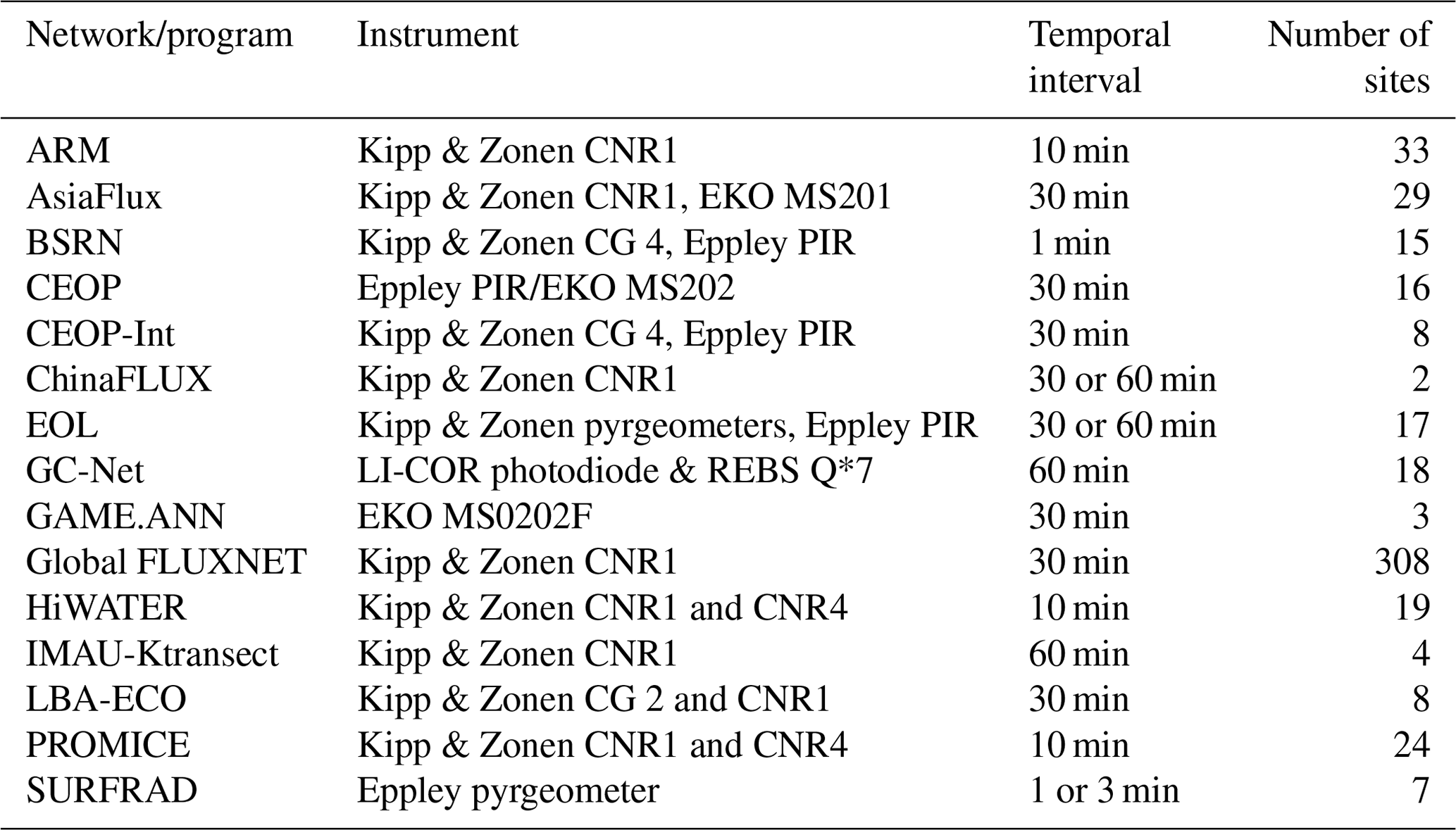
Ground measurements of daily surface Rn were used for the RCNN model development. The in situ measurements used in this study cover the period from 2001 to 2019 and were obtained using various instruments (e.g., Kipp & Zonen CNR1 and Eppley) at 522 globally distributed stations from 15 observation networks/programs, as shown in Fig. 1. Detailed information about these observation networks/programs is listed in Table 2, and specific information about these sites is shown in Table S1 in the Supplement. These stations are maintained by multiple global and regional observation network organizations, such as the global FLUXNET, the Greenland Climate Network (GC-Net), and the Programme for Monitoring of the Greenland Ice Sheet (PROMICE) (Jiang et al., 2018). These stations vary in elevation from 4 to 5063 m above sea level and are located in areas with different land cover types, including forest, grassland, shrubland, wetland, cropland, ice/snow, and urban areas. The collective in situ measurements, therefore, represent an accurate and comprehensive dataset that is capable of accounting for surface Rn spatial–temporal variation on a global scale.
The instruments applied to obtain surface radiation have different uncertainties. To be specific, the operational thermoelectric pyranometers are known for their high-accuracy performance, with a spectral response of 0.3–3.0 µm, a sensitivity of 7–14 µV W−1 m2, a thermal effect of less than 5 %, and an annual stability of 5 % (Lu et al., 2011; Jiang et al., 2019b). Eppley precision infrared radiometers (PIRs, 3.5–50 µm) and Kipp & Zonen CG 4 pyrgeometers (4.5–42 µm) are applied to measure the surface radiation with an uncertainty of ±6 % or 15 W m−2 at the 95 % confidence level (Philipona et al., 1998). The largest uncertainties for surface radiation measurements are ∼ 2 % for pyrheliometers and ∼ 5 % for pyranometers (i.e., 15 W m−2), respectively (Augustine et al., 2000). Additionally, the radiation measurements obtained by Kipp & Zonen CNR1 and CNR4 instruments are with an expected accuracy of ±10 % for daily totals (Wang and Dickinson, 2013). The radiation observations measured by Kipp & Zonen net radiometers (CNR1, 5–50 µm, or CNR1-lite, 4.5–42 µm) are with uncertainty of ∼ 10 % at the 95 % confidence level for daily totals (Yamamoto et al., 2005). Besides, the uncertainties in the shortwave radiation measured by a LI-COR photodiode and Rn observed by REBS Q*7 are about 5 (5 %–15 %) and 10 W m−2 (5 %–50 %), respectively, at a monthly timescale (Box and Rinke, 2003; Steffen and Box, 2001). To deal with equipment and operational errors, daily mean surface Rn measurements were calculated based on several strict processing rules successfully applied in previous studies (Jia et al., 2018; Jiang et al., 2014; Chen et al., 2020; Jiang et al., 2018).
To well illustrate the performance of the model in estimating global surface Rn, more sites from international observation networks should be determined as the validation sites rather than regional observation networks with similar climate regimes (e.g., Atmospheric Radiation Measurement, ARM) to ensure the independence of the test dataset, which avoids overfitting in model training. In this study, more than 89 % of validation sites come from the continental and international networks, including the Baseline Surface Radiation Network (BSRN), FLUXNET, the Coordinated Enhanced Observation Network of China (CEOP), Earth Observing Laboratory (EOL), AsiaFlux, and PROMICE. Additionally, similar and comprehensive surface and atmospheric conditions between the training and validation sites illustrate the good representations of both the training and the independent test datasets in global surface Rn variability (Fig. S1 in the Supplement), which detects the ability of the model in estimating global surface Rn. Note that some current regional and international networks are interconnected; for example, some ARM and all BSRN sites are included in the BSRN networks. When determining the training and validation sites, more attention should be paid to these duplicate sites in multiple observation networks to ensure the independence of the validation sites from the training sites. Finally, as shown in Fig. 1, the surface Rn measurements from 448 stations were used to train the proposed RCNN model (red circles), while the measurements from the remaining 75 stations (blue circles) were selected as the independent test dataset to evaluate the model performance.
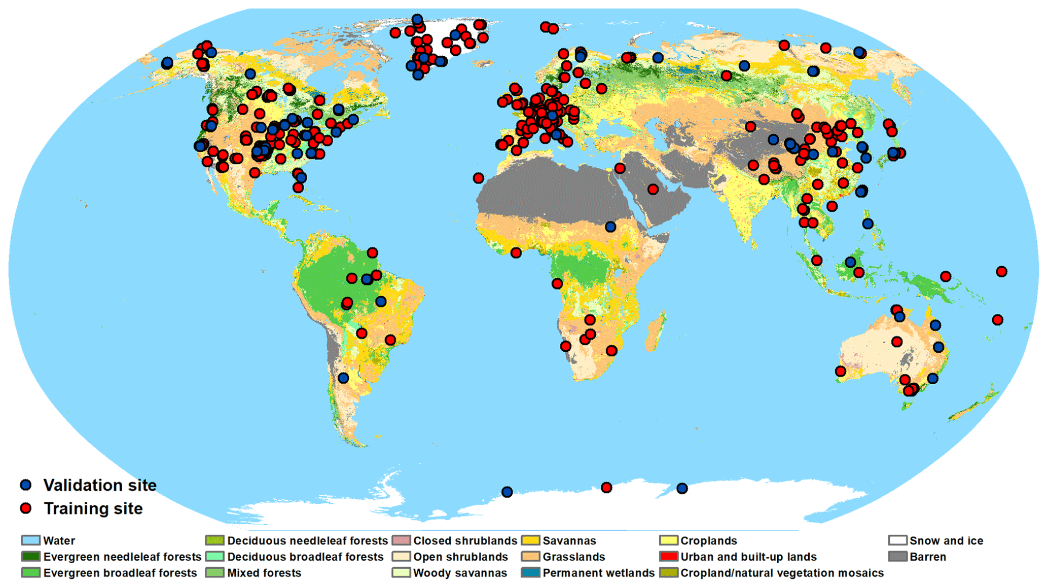
Figure 1Geographic locations of the 522 ground stations used in this study. The 448 stations marked with red circles are used to train the RCNN model, while the other 74 stations marked with blue circles are used for the independent validation of the resulting trained model. Background colors indicate different land cover according to the International Geosphere-Biosphere Programme (IGBP) classification system.
Table 2Information about the observation networks. ARM: Atmospheric Radiation Measurement; BSRN: Baseline Surface Radiation Network; CEOP-Int: Coordinated Enhanced Observing Period; CEOP: Coordinated Enhanced Observation Network of China; EOL: Earth Observing Laboratory; GAME.ANN: GEWEX Asian Monsoon Experiment; GC-Net: Greenland Climate Network; IMAU-Ktransect: Institute for Marine and Atmospheric Research Ice and Climate; LBA-ECO: Large-Scale Biosphere-Atmosphere Experience; PROMICE: Programme for Monitoring of the Greenland Ice Sheet; SURFRAD: Surface Radiation Budget Network.
2.2 AVHRR data
AVHRR TOA observations at five spectral channels (a visible band (0.55–0.68 µm), a near-infrared band (0.75–1.1 µm), a middle-infrared band (3.55–3.93 µm), and two thermal bands (10.5–11.3 and 11.5–12.5 µm)) were utilized for their comprehensive surface and atmospheric electromagnetic information. The National Aeronautics and Space Administration (NASA) Land Long Term Data Record (LTDR) project produced a consistent long-term dataset by reprocessing Global Area Coverage (GAC) data, which were obtained from AVHRR sensors on board the National Oceanic and Atmospheric Administration (NOAA) satellites (Pedelty et al., 2007). The primary reprocessing improvements included radiometric in-flight vicarious calibrations for the visible and near-infrared channels, along with inverse navigation to relate a specific Earth location to each sensor's instantaneous field of view (Vermote and Kaufman, 1995; Pedelty et al., 2007). Multiple Climate Modeling Grid (CMG) data from AVHRR and MODIS instruments have been created for land climate studies (Xiao et al., 2017; Pedelty et al., 2007). In this study, we utilized a daily AVHRR TOA data product (AVH02C1) with a resolution of 0.05∘ from 1981 to 2019 to retrieve surface Rn estimates. Additionally, solar and viewing geometry data (i.e., SZA, VZA, and RAA) were also incorporated into the model as the amount of solar radiation incident on the Earth's surface varies greatly under different geometric observation conditions. A summary of these gridded products and their attributes is presented in Table 3.
Table 3List of the satellite and reanalysis products used in this study.

2.3 GLASS product
The GLASS daily surface Rn product from MODIS data, one part of the GLASS product suite (Liang et al., 2020), was produced using two sets of algorithms. The main algorithm primarily uses the well-documented conversion relationships between downward shortwave radiation and all-wave Rn combinations (Wang and Liang, 2009; Jiang et al., 2015). It also incorporates a combination of other meteorological variables under various environmental conditions, such as different daytime lengths and land cover characteristics, which are designated based on the albedo and normalized difference vegetation index (NDVI). Multiple multivariate adaptive regression splines (MARS) learners were employed to establish efficient statistical relationships using GLASS downward shortwave radiation and MERRA-2 meteorological variables, allowing land surface Rn to be estimated from these inputs across most spatial domains (Jiang et al., 2016, 2015). Conversely, when surface solar radiation data were not available, the backup algorithm created a function that separately employed MODIS TOA observations to retrieve surface all-wave Rn using the length ratio of daytime (LRD) classification method, which was accomplished by the genetic algorithm–artificial neural network (GA-ANN) (Chen et al., 2020). By using these two algorithms, the GLASS Rn product can provide seamless global land surface Rn estimates with a 0.05∘ resolution. Several studies have used in situ measurements to conduct evaluation studies, illustrating high-accuracy performance as well as good application potential (Jiang et al., 2018; Guo et al., 2020). Thus, we used the GLASS daily Rn product covering 2000 to 2018 as a reference to help select reliable sites and validate the results from this study.
2.4 CERES-SYN product
The CERES instruments on board the Terra, Aqua, and Suomi National Polar-orbiting Partnership (Suomi NPP) satellites observe the TOA global energy budget by measuring shortwave reflected radiation, longwave Earth-emitted radiation, and all wavelengths of radiation at a spatial resolution of 20 km at nadir (Wielicki et al., 1996). The CERES Synoptic (CERES-SYN) product combines CERES and MODIS observations with geostationary (GEO) data to provide hourly broadband TOA radiant flux and cloud properties (Doelling et al., 2013). The CERES-SYN product also contains computed TOA and in-atmosphere and surface fluxes based on the Fu-Liou radiation transfer model. Aerosol and atmospheric data were included as inputs to calculate the radiation flux. CERES-SYN fluxes were provided as a 1∘ gridded product with an hourly temporal resolution. CERES-SYN surface Rn data have been evaluated in many studies, which indicate that the product has high accuracy, although systematic overestimation exists in the surface net radiation flux data (Jia et al., 2018; Jiang et al., 2016; Jia et al., 2016). Thus, the CERES-SYN surface Rn obtained from four surface radiative components was used as a reference for comparison.
2.5 MERRA-2 reanalysis
MERRA-2, produced by the NASA Global Modeling and Assimilation Office (GMAO), is the latest global atmospheric product and employs satellite observation data from 1980 to the present. The MERRA-2 reanalysis assimilates space-based observations of aerosols and represents their interactions with other physical processes in the climate system. The goals of MERRA-2 are to provide a regularly gridded, homogeneous record of the global atmosphere and to incorporate additional climatic variables and conditions, including trace gas constituents (stratospheric ozone), improved land surface representation, and cryospheric processes (Gelaro et al., 2017b). The MERRA-2 products have a 0.5∘ × 0.625∘ spatial resolution and hourly temporal resolution. Previous studies (Jiang et al., 2018; Jia et al., 2018; Delgado-Bonal et al., 2020) have confirmed that the MERRA-2-calculated surface Rn and its radiative component provide outstanding accuracy and a reasonable spatial–temporal distribution compared to other reanalysis data. Therefore, MERRA-2 Rn data calculated from four surface radiative components were also used in this study to help retrieve accurate high-resolution surface Rn estimates by providing average atmospheric information.
The entire workflow of the RCNN-based PSME method is shown in Fig. 2. First, the ETC technology was applied to the triplet system constructed from ground-, satellite-, and model-based Rn data to identify reliable sites at which measurements can well represent the dynamic variation in surface Rn at a 5 km scale. Then, AVHRR TOA reflectance, brightness temperature, angular information, and MERRA-2 Rn were matched with the ground-based Rn measurements, both spatially and temporally. Specifically, the site-measured Rn data were collocated with the 5 km AVHRR grid product covering the site. If one grid in the AVH02C1 product covered multiple sites, the mean values from these sites' measurements were used to match the grid data. Subsequently, the matched input–output training samples were fed into the RCNN to train the model. Reference Rn measurements taken from reliable sites were used to evaluate the model's performance and, subsequently, identify the best option to produce surface Rn by tuning the hyper-parameters of the RCNN. Finally, surface Rn retrievals were generated using the best-trained model for the global scale, and CERES-SYN and GLASS Rn products were applied to perform inter-comparisons to illustrate the accuracy and spatiotemporal variation in the surface Rn retrievals.
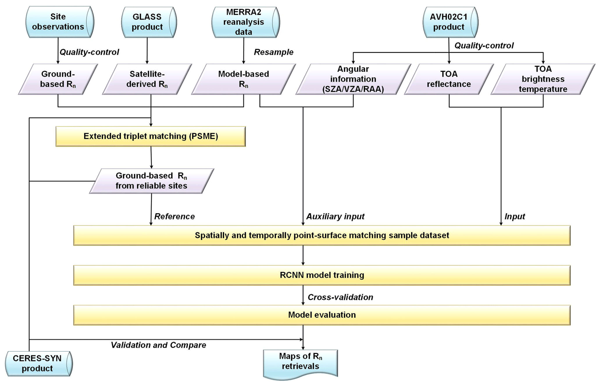
Figure 2Workflow of RCNN-based point-surface matching estimation (PSME) method for surface Rn retrievals. TOA: top of atmosphere; RCNN: residual convolution neural network; GLASS: Global Land Surface Satellite; CRES-SYN: Clouds and the Earth's Radiant Energy System Synoptic; MERRA2: Modern-Era Retrospective analysis for Research and Applications, Version 2; SZA: solar zenith angle; VZA: viewing zenith angle; RAA: relative azimuth angle.
3.1 Extended triple collocation (ETC)
To address the spatial-scale mismatch issue owing to the small spatial support of sparse ground measurements in comparison to gridded satellite data, which introduces large uncertainty into the collaborative inversion process, triplet collocation (TC) technology was employed (Stoffelen, 1998; Yuan et al., 2020a). Specifically, based on the availability of three collocated, independent measurement systems describing the same geophysical variable, TC was designed to estimate the unknown error standard deviations (or root-mean-square errors, RMSEs) of three mutually independent measurement systems, without treating any one system as perfectly observed “truth” (Stoffelen, 1998; Gruber et al., 2016). To perform the TC, the following assumptions were made: (1) each of the triplets is related to the unknown truth of the geophysical variable in the linear form; (2) there is zero cross-correlation across each of the triplets; (3) there is zero error cross-correlation between the triplet and the true signal state (T); and (4) the signal and error statistics are stationary (Chen et al., 2017). Following the first assumption, the independent triplet systems (Xi, Xj, and Xk) are related to the unknown true quantity in a linear error model:
where αi and βi are the additive and multiplicative bias terms, respectively, and εi is the mean-zero random error. Similar calibration constants (αj, βj, αk, and βk) and random error terms (εj and εk) are also defined for Xj and Xk.
The objective of TC is to find a solution that individually estimates the variance of the random error term (εi) for each of the triplets based on the listed assumptions (Stoffelen, 1998; Yuan et al., 2020a). However, to obtain the calibration constants, one dataset is chosen from the three collocated measurement systems as the reference dataset, and the other two are rescaled into the same reference data space. This results in a dependency of the error variance of the other two datasets on the climatology of the scaling reference (Draper et al., 2013; Yuan et al., 2020a). To deal with this issue, ETC technology was proposed by McColl et al. (2014), based on the same assumptions as TC, to estimate an additional evaluation metric independent of the reference dataset, i.e., a correlation coefficient () of each measurement system with respect to the unknown target variable as formulated below:
where is correct up to the sign ambiguity, as the measurement systems will almost always be positively correlated to the unobserved truth.
Following the ideals of Chen et al. (2017) and Yuan et al. (2020a), ETC was applied to determine the reliable site measurements over the AVHRR data footprint scale (i.e., 5 km grid). Specifically, the triplet dataset was first constructed using ground-based measurements (i.e., site measurements), satellite-derived retrievals (GLASS Rn), and downscaled model-based simulations (MERRA-2 Rn) depending on the conversion ratio of GLASS Rn between original (0.05∘) and aggregated (0.5∘) spatial resolutions, as they belong to different measurement systems and are not dependent on each other. Then, was calculated using Eq. (2) for individual sites, illustrating the fraction of 5 km satellite footprint-scale Rn dynamics captured by point-scale ground-based measurements. An appropriate threshold of was determined to select reliable sites with the greatest representativeness within a 5 km footprint to obtain sample datasets for the model training. After testing a series of thresholds between 0.2 and 0.9 at intervals of 0.1, a threshold of 0.9 was selected, above which the sites were assigned as “reliable” (also see Sect. 5). Based on these reliable sites, errors in upscaling reliable site-based measurement to a 5 km scale can be weakened to a certain degree due to the measurement's better representativeness within the AVHRR footprint.
3.2 RCNN-based PSME
3.2.1 RCNN
As the spatial resolution of satellite sensors increases, the spatially adjacent effects induced by spatially inhomogeneous atmospheric constitute (or cloud) fields become more significant; for example, clouds affect the distribution of surface radiation in a region larger than the resolution of an individual pixel. One spatially adjacent effect is the diffusion of radiation that removes part of radiation from an atmospheric column and transfers it to neighboring columns. Two other effects are related to the solar and viewing geometry, such as a shift of the apparent position of clouds and their shadows. Surface Rn is no longer accurately estimated with retrieval algorithms based on the individual pixel approximation (IPA). Comprehensive information within a certain spatial extent centered at reliable sites needs to be considered to help retrieve surface Rn.
Loosely inspired by the human visual cortex, CNNs were originally applied to analyze common visual imagery using convolution instead of general matrix multiplication (Ball et al., 2017). A CNN model can extract features hierarchically from multi-channel input images using multiple filters. Therefore, the most important feature information regarding reliable site-based Rn measurements can be effectively extracted by CNNs within a certain spatial extent rather than on the basis of IPA, to help retrieve Rn, which weakens the spatially adjacent effects to a certain extent. A general CNN consists of multiple layers of operations, such as convolution, pooling, normalization, and nonlinear activation functions. In the convolutional layers, a series of convolution (Conv) operations are performed using convolutional kernel weights and biases on the input images within the receptive field. The result of the locally weighted sum (feature map) is then passed through a nonlinear layer, such as a rectified linear unit (ReLU), which increases the nonlinear properties of the decision function and the overall network (Romanuke, 2017). The pooling layer, a form of nonlinear down-sampling, merges semantically similar features into one, thereby reducing the amount of computation in the network (Géron, 2019). Additionally, a batch normalization layer is placed between the convolutional layers and nonlinearities to speed up the training of the CNN and reduce the sensitivity to network initialization. By stacking two or three stages of convolution, nonlinearity, and pooling, followed by more fully connected layers, a typical CNN architecture is built.
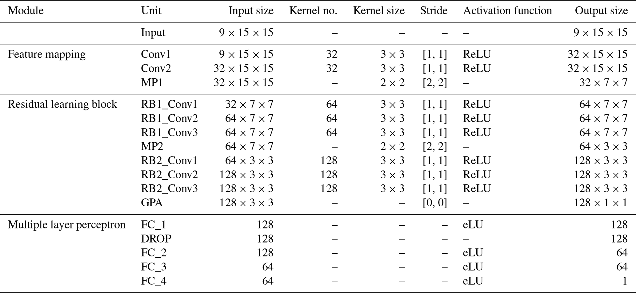
To improve network performance in complicated tasks, a deeper CNN architecture is needed; however, a deeper neural network is difficult to train well because a degradation problem occurs when deeper networks converge (He et al., 2016). Specifically, as the network depth increases, the training accuracy becomes saturated and then degrades rapidly. To address the degradation problem, He et al. (2016) proposed a residual block to improve the gradient flow through the network, which enables the training of deeper networks. Residual blocks were employed in our CNN architecture to construct the RCNN. The structure of the RCNN proposed in this study is shown schematically in Fig. 3. Table 4 lists the detailed configurations of the proposed RCNN.
The input signals of the RCNN included AVHRR TOA reflectance and brightness temperature, angular information (SZA, VZA, and RAA), and daily MERRA-2 Rn with a spatial size of 15 × 15 pixels (these specifications are further discussed in Sect. 5). To avoid introducing new errors, nearest-neighbor interpolation was used to resample MERRA-2 Rn to 0.05∘ to match the spatial resolution of the other predictors. The output signal was ground-based Rn from the reliable sites. Essentially, the RCNN model uses a convolution operation taken at stages of the feature map and residual learning block to recognize spatial patterns centered on a reliable site. Then, the multiple layer perceptron links abstract spatial patterns with ground-based measurements to construct a strong nonlinear relationship to reproduce the spatial and temporal variation in surface Rn. This approach had been carried out in previous studies (Jiang et al., 2019b, a, 2020a).
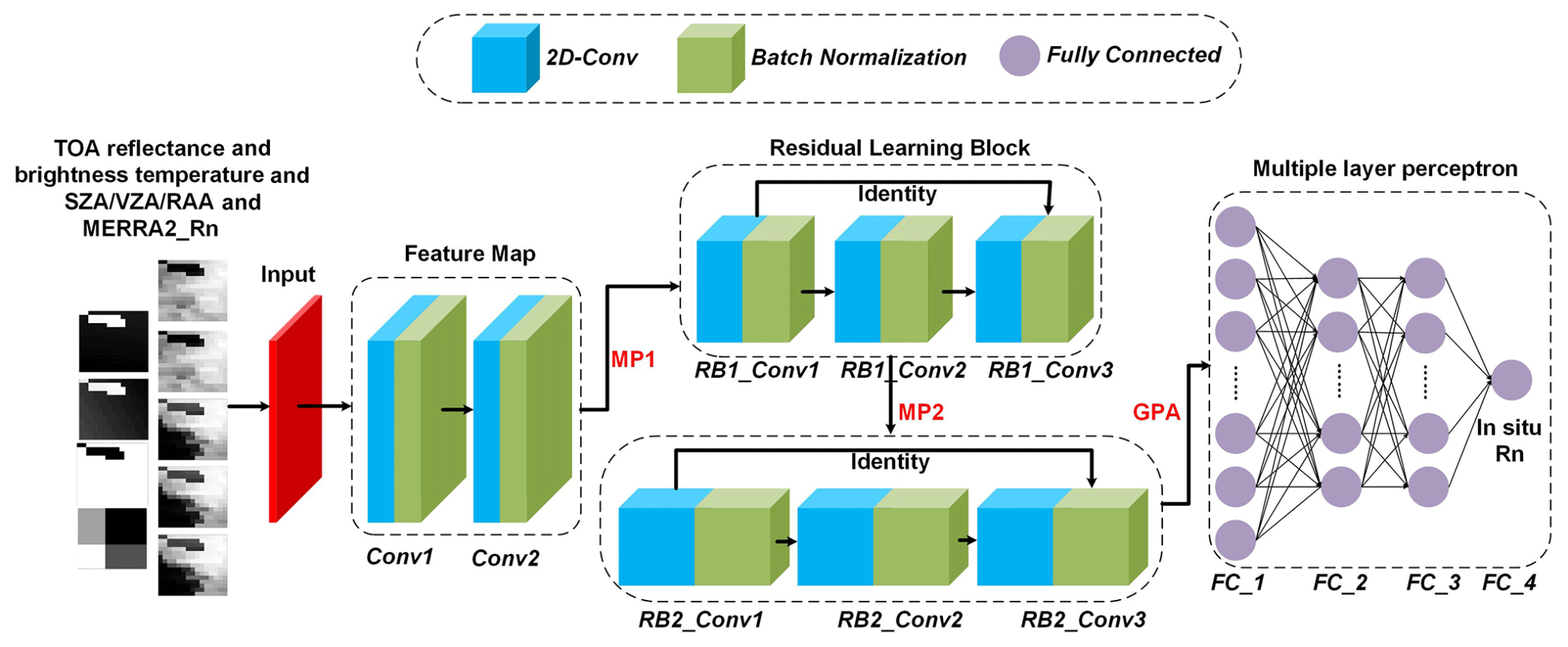
Figure 3Depiction of the RCNN. The model uses AVHRR TOA observations, angular information (SZA, VZA, and RAA), and MERRA-2 Rn as inputs, which are used to calculate daily surface Rn values as output. Conv represents the convolution operation; MP and GPA are the max-pooling and global average-pooling operations, respectively; RB: residual block; FC: fully connected layer.
Table 4Detailed configuration of the RCNN. eLU: exponential linear unit; DROP: dropout layer.
3.2.2 RCNN model training and evaluation
Sample data from the reliable sites in the training site group (red circles shown in Fig. 1) were used to train the RCNN model; datasets from reliable sites in the independent validation site group (blue circles shown in Fig. 1) served as test datasets to independently evaluate the model's performance. Specifically, in the training process, 10-fold cross-validation (CV) was used to test the model's predictive power. All of the sample datasets from the reliable training sites were randomly shuffled and divided into 10 groups. One group of these data was then removed as a hold-out or validation dataset, and the remaining nine groups of data were treated as the training datasets. The training datasets were used to fit the RCNN model, and the validation datasets were applied to evaluate the trained model's performance to fine-tune the model's parameters. The process was repeated 10 times to ensure that each group of data validated the model, and the remaining nine groups of data were trained. Finally, the evaluation results were presented by summarizing and averaging the 10 evaluation scores. After determining the hyper-parameter settings using the CV, the model was trained again using datasets from all the reliable training sites, which was then independently evaluated using the test datasets from the reliable validation sites.
The following five evaluation metrics were used to evaluate the performance of the RCNN model and the Rn retrievals: bias, relative bias (rbias), RMSE, relative RMSE (rRMSE), and the coefficient of determination (R2). Detailed information regarding the application of these metrics can be found in Yang et al. (2018).
4.1 Identification of reliable sites
The number of reliable and unreliable sites for each observation network, identified by a threshold of 0.9 for the ETC-derived correlation coefficient, is listed in Table 5. A total of 262 sites could be considered reliable, accounting for ∼ 50 % of the sites. Furthermore, no site was considered reliable for some observation networks/programs, namely ChinaFLUX, GC-Net, GAME.ANN, HiWATER, IMAU-Ktransect, and LBA-ECO. It is not surprising that sites from the ChinaFLUX network were assigned as unreliable; several studies have revealed that the reliability of site measurements from China is questionable and should be examined carefully before use (Zhang et al., 2015; Tang et al., 2013, 2011). GC-Net is located in inner Greenland, where systematic measurements errors are common due to difficulties in instrument maintenance and operation-related failures. Sites from the GAME.ANN network are located in the Tibetan Plateau (TP) region, where abnormal climate and complex terrain make it difficult to accurately measure variations in Rn. Similar issues also exist in in situ measurements from the IMAU-Ktransect, HiWATER, and LBA-ECO networks. In contrast, some of the international observational networks, such as BSRN (Ohmura et al., 1998) and FLUXNET (Wilson et al., 2002), provide many ground-based measurements with sufficient spatial representativeness for Rn at a 5 km resolution. In addition, the ARM (Stokes and Schwartz, 1994) and SURFRAD (Augustine et al., 2000) networks were classified as containing reliable sites. In situ measurements from the SURFRAD (Augustine et al., 2000) network were well known in surface radiation budget studies because of their high data quality and have been widely utilized as a result (Wang et al., 2015b; Hao et al., 2019; Wang et al., 2015a; Qin et al., 2012). Overall, compared to other networks, the sites from ARM, BSRN, SURFRAD, and FLUXNET networks were mostly identified as reliable sites, illustrating the superiority of these observation networks.
The spatial and proportion distributions of the reliable training and validation sites for different surface types are presented in Fig. 4. The most reliable sites are distributed in the United States, Europe, and East Asia. In turn, many sites located in South America, Africa, Eurasia, and the polar regions were identified as unreliable. The reasons for these sites being classified as unreliable are closely related to the complex surface and atmospheric environment and poor instrument maintenance in their corresponding regions. Most grassland and cropland sites were classified as reliable (∼ 66 % and ∼ 62 %, respectively), whereas the fewest reliable sites were classified in ice-/snow-covered areas (∼ 14 %). In addition, sites neighboring the sea were mostly identified as unreliability due to the presence of large water bodies within the satellite footprint. Thus, the processing of identifying reliable sites highlights the need to pay more attention to such areas for surface radiation estimations.
Table 5Summary of the selected reliable and unreliable sites based on ETC for each observation network.

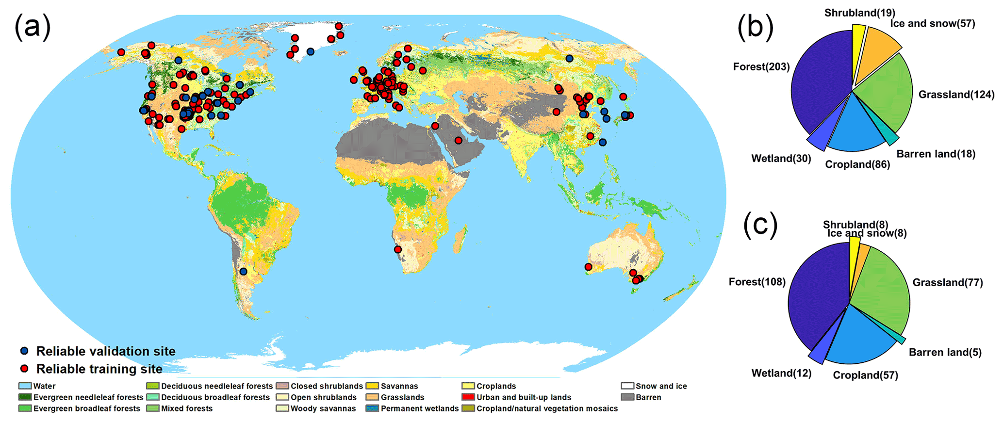
Figure 4(a) Spatial distribution of reliable sites and the absolute numbers of (b) all sites and (c) reliable sites under different surface types.
4.2 Assessment of the RCNN model
Ten-fold CV was used to evaluate the performance of the RCNN model at reliable and all training sites, and the evaluated performances are summarized in Table 6. Note that the model fitting result represents the model with the best-fitting accuracy over the 10 CV rounds, while the cross-validation results are the averages of the 10-round combination. The RCNN model showed a high fitting accuracy at the reliable training sites with R2, RMSE (rRMSE), and bias (rbias) values of 0.90, 20.61 W m−2 (25.71 %), and 0.42 W m−2 (0.53 %), respectively. Compared to the model fitting accuracy across all sites, the result for the reliable sites was improved, with R2 values increased by 0.04 and rRMSE values reduced by 8.24 %. The implementation of ETC for the selection of reliable sites ensures more consistent spatial representativeness of ground-based measurements and AVHRR data, which improves the accuracy of Rn retrievals. Indeed, the CV-derived average accuracy is extremely similar to the model fitting accuracy, illustrating that the trained RCNN model is highly robust. Additionally, an unbiased estimation was achieved by the RCNN model with CV-derived biases close to zero.
Figure 5 shows the overall training accuracy and test accuracy for the RCNN model at reliable training and independent validation sites. The over-training accuracy of the RCNN model is close to that of the CV-derived result. Between the model training to the test phase, the R2 score dropped by 0.06 and RMSE increased by 5.93 W m−2 (5.96 %), which indicates slight overfitting by the proposed model. However, with the highest cross-validated R2 of 0.90 and the lowest RMSE of 21.01 W m−2, the RCNN model trained using ground-based Rn measurements obtained at the reliable sites is considered the best-trained model, which was selected for the subsequent analysis.
Table 6Ten-fold cross-validation performance of the RCNN models.
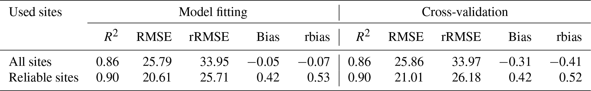

Figure 5Scatterplots of (a) model training (fitting) accuracy and (b) model test accuracy for the reliable training and independent validation sites. The color bar illustrates the normalized density of samples.
4.3 Evaluation of the RCNN-based AVHRR Rn retrievals
4.3.1 Inter-comparisons of Rn products
Figure 6 shows the validation results of the four datasets at the reliable sites, including the AVHRR, CERES-SYN, MERRA-2, and GLASS Rn estimates. Comparatively, the RCNN-derived AVHRR Rn retrievals show the best performance with R2, RMSE, and bias of 0.90, 21.08 W m−2 (26.22 %), and −0.38 W m−2 (−0.47 %), respectively, followed by the GLASS Rn estimates with corresponding values of 0.89, 22.47 W m−2 (27.95 %), and −2.96 W m−2 (−3.68 %), respectively. The CERES Rn estimates show a notable overestimation at higher values against the in situ measurements with a bias of 7.25 W m−2 (9.04 %). In addition, a greater uncertainty exists in the CERES Rn compared to the AVHRR and GLASS Rn estimates, with an RMSE of 25.11 W m−2. The CERES-SYN cloud product, an input for the calculation of flux products, underestimated low-level clouds (by 11.8 % and 20.9 % for day and night, respectively) over the sun-glint ocean and polar regions during both the daytime and the nighttime (Xi et al., 2018; Xu et al., 2020). Additionally, when the aerosol optical depths (AODs) used to calculate CERES-SYN surface solar radiation are compared with the ground-based observations, the calculated shortwave radiation is 1 %–2 % higher (Fillmore et al., 2021). Therefore, large uncertainties in these atmospheric input parameters may lead to serious overestimations of the CERES-SYN Rn. In addition, the MERRA-2 Rn shows the lowest accuracy, with an RMSE of 30.88 W m−2, reflecting the reanalysis model's inability to accurately describe the evolution of cloud properties (Betts et al., 2006). Comparatively, the AVHRR retrievals show a better accuracy than the other three products. In addition, our estimates have a higher spatial resolution compared to the CERES-SYN and MERRA-2 data.
Compared to the validation results at the reliable sites, the accuracy evaluation at all sites shows the ability of the RCNN to accurately capture Rn variation at a global scale, even though some measurements from unreliable sites added large uncertainties to the final evaluation. Figure S2 shows a comparison of results for the four datasets at all of the sites. Overall, the AVHRR and GLASS Rn retrievals were still better than those of CERES-SYN and MERRA-2; however, the accuracy of AVHRR Rn decreases slightly, with R2, RMSE, and bias values of 0.85, 26.74 W m−2 (35.70 %), and 1.20 W m−2 (1.60 %), which is comparable to the GLASS Rn retrievals, with values of 0.85, 26.79 W m−2 (35.77 %), and −0.82 W m−2 (−1.10 %), respectively. Therefore, even if the RCNN model is trained using measurements from less reliable sites, it still accurately reproduces surface Rn distributions at the global scale. In the following analysis, the GLASS Rn retrievals were used as the main comparison because of their high accuracy and reasonable spatiotemporal variation (Jia et al., 2018; Jiang et al., 2018).
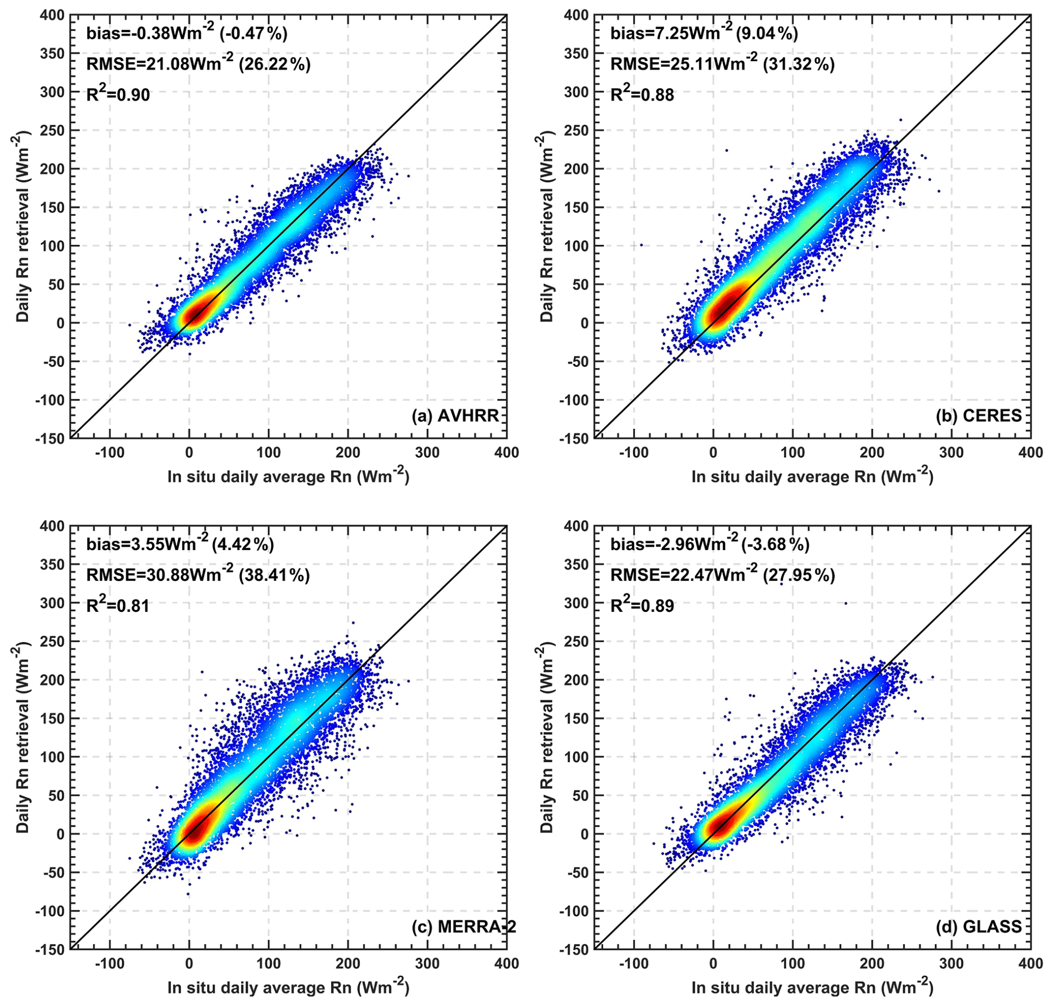
Figure 6Scatterplots of product validation for (a) AVHRR, (b) CERES-SYN, (c) MERRA-2, and (d) GLASS at the reliable sites.
Inter-comparison results for the AVHRR and GLASS Rn retrievals against the ground-based measurements over each network are displayed in Fig. 7. The AVHRR Rn retrievals performed slightly better than the GLASS Rn retrievals in most of the observation networks. Specifically, the AVHRR Rn retrievals show lower RMSE values over seven networks, except for the EOL and PROMICE networks. However, the RMSE differences over the EOL and PROMICE networks are very small – only 1.41 and 0.22 W m−2, respectively. The EOL is a small regional network, and its measurements thus only reflect local-scale Rn variation. However, only 2 out of 17 sites were identified as reliable for the model training and, therefore, the RCNN model cannot capture specific Rn dynamics within such a small spatial extent. Similar reasons also account for the poor performance for the PROMICE network because most of the sites in the GC-Net and PROMICE networks are identified as unreliable sites. Thus, the RCNN model has less knowledge of Rn dynamics for snow and ice surfaces. The most significant difference for RMSE was observed over the ARM network, for which the mean RMSE value decreased by 2.0 W m−2 for the AVHRR Rn retrievals relative to the GLASS Rn retrievals. Additionally, these two datasets showed very similar performance based on their R2 values.

Figure 7The average performance of the AVHRR and GLASS Rn retrievals against ground-based measurements at the reliable sites over each network.
To further improve understanding of the temporal variations in the AVHRR Rn retrievals, coincident time series from all the Rn datasets were inter-compared over seven sites representing different surface types, as shown in Fig. 8. Overall, all four datasets broadly captured the true dynamics of Rn under the different surface types. Comparatively, the AVHRR and GLASS Rn retrievals are more consistent with in situ measurements than the CERES-SYN and MERRA-2 products. Specifically, the MERRA-2 and CERES-SYN Rn retrievals show higher values compared to the in situ measurements at the BSRN_DRA site, especially during the 140–200 d period. In comparison, the AVHRR and GLASS Rn values closely match the ground-based measurements and thereby better reflect the true temporal variation in Rn. At the Lath_UK-AMo site, four of the datasets slightly overestimated Rn compared to in situ measurements during the summer; however, the AVHRR and GLASS Rn retrievals still performed best. Moreover, large discrepancies occurred at the PM-SCO_U site under the snow/ice surface for the four datasets. Notably, MERRA-2 Rn values do not reflect true variations for snow and ice surfaces, especially during the 150–250 d period. Comparatively, the satellite-derived retrievals better capture Rn dynamics, although the CERES-SYN product still exhibits overestimation. Because less reliable sites were screened at the global scale to train the RCNN model under the snow/ice surfaces, the AVHRR Rn values only capture the general Rn trend in the snow/ice areas. The GLASS Rn retrievals are also most consistent with the in situ measurements among the four datasets, although small biases still exist.
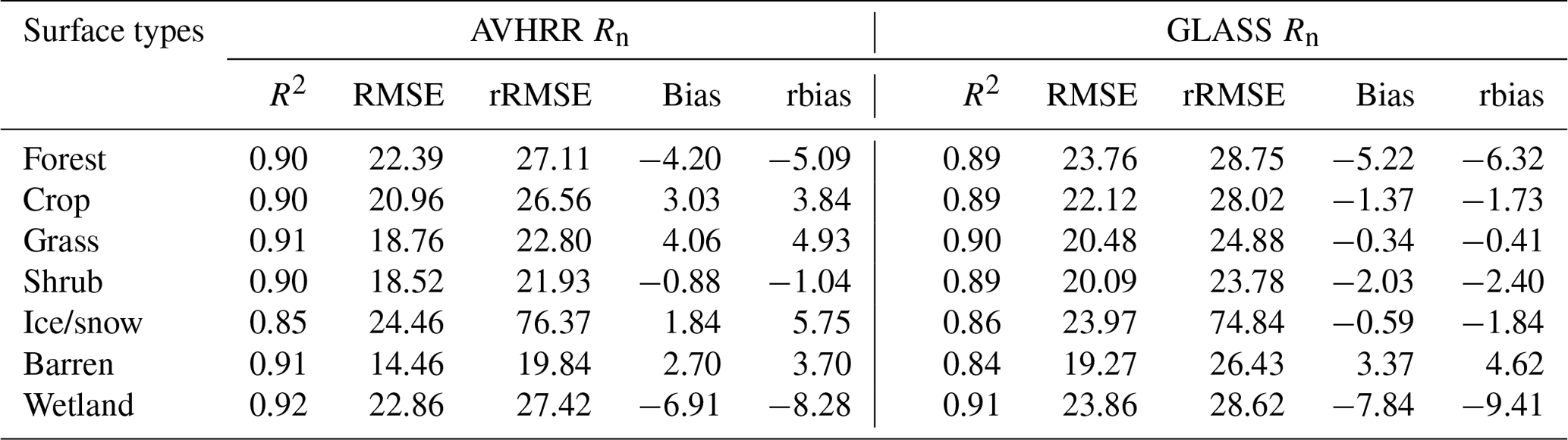
The overall evaluation results of the AVHRR and GLASS Rn retrievals for different surface types are displayed in Table 7. Generally, both datasets achieved high accuracy, with RMSEs ranging from 20 to 25 W m−2. The AVHRR Rn retrievals show the better performance for most of the surface types, except for snow/ice, as previously discussed; however, the difference in the RMSEs between the AVHRR and GLASS Rn retrievals for the snow/ice cover type is small (0.49 W m−2). Together, these results further indicate that the RCNN model can generate accurate Rn estimates for different land cover types.
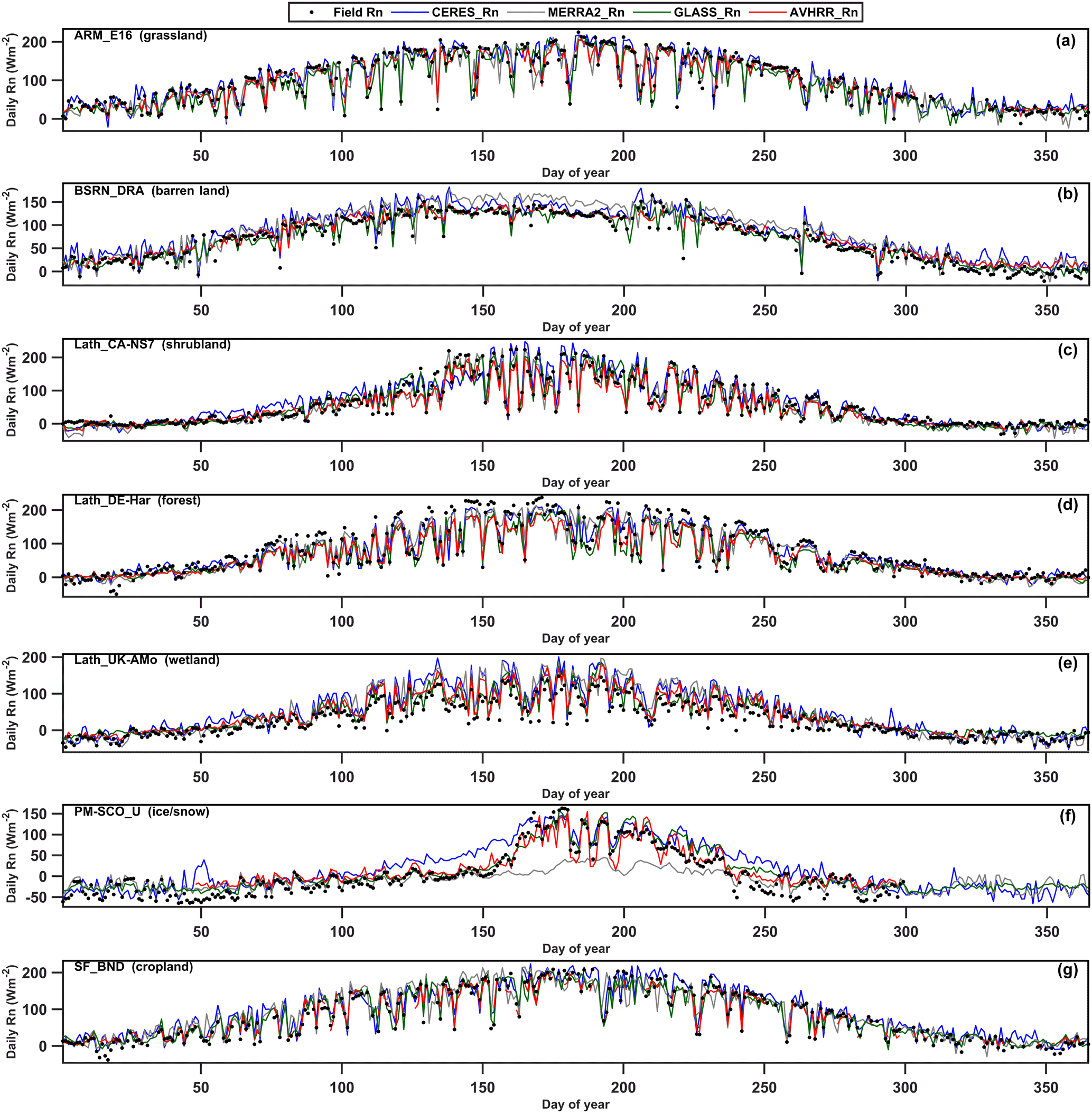
Figure 8Coincident time series of the AVHRR, GLASS, MERRA-2, and CERES-SYN Rn retrievals and ground-based measurements over seven sites representing different surface cover types for (a) ARM_E06 (38.061∘, −99.134∘), (b) BSRN_DRA (36.626∘, −116.018∘), (c) Lath_CA-NS7 (56.635∘, −99.948∘), (d) Lath_DE-Har (47.934∘, 7.601∘), (e) Lath_UK-AMo (55.791∘, −3.238∘), (f) PM-SCO_U (72.393∘, −27.233∘), and (g) SF_BND (40.050∘, −88.37∘).
Table 7Evaluation of the AVHRR and GLASS Rn retrievals for different surface cover types.
4.3.2 Analysis of influencing factors
Variation in surface Rn is mainly affected by atmospheric conditions but also, to a lesser degree, by surface characteristics (He et al., 2015). Under clear-sky conditions, AOD and column water vapor (CWV) are the main atmospheric constituents that modulate surface shortwave and longwave radiation and further affect spatiotemporal variations in surface Rn. In contrast, clouds and CWV control surface Rn dynamics under cloudy-sky conditions, especially clouds that have significant impacts on shortwave and longwave radiation. Therefore, AOD, CWV, and cloud optical thickness (COT, as a surrogate for cloud optical properties) derived from MERRA-2 were employed to analyze the sensitivity of the accuracy of the AVHRR and GLASS Rn retrievals to variations in these influencing factors. In addition, Rn retrieval performance at different elevations was also evaluated.
All the evaluation results are displayed in Fig. 9. The AVHRR Rn retrievals were always better than the GLASS Rn retrievals under all conditions of the four influencing factors, except for elevations ranging from 800–1000 and 1200–1500 m, which demonstrates the superiority of our algorithm. Specifically, as the COT increases (i.e., increasing cloud thickness), the AVHRR and GLASS Rn RMSE values increase accordingly but still remain relatively low for both datasets (< 27 W m−2). Note that the differences in RMSE between the two datasets also increased with increasing COT (Fig. 9a). A small COT indicates relatively clear-sky conditions, which results in surface total solar radiation dominated by direct solar radiation. Therefore, the performance of the RCNN model and the MARS models used for the GLASS Rn product (Jiang et al., 2016) is comparable with regard to the accuracy of their Rn retrievals. However, when the absorption and scattering effects are enhanced for direct solar radiation from TOA, depending on the IPA, it is difficult to retrieve the total surface Rn accurately using the MARS model because the spatially adjacent effects (i.e., 3-D effects from clouds) are not considered. Although the RMSEs of the AVHRR retrievals also increase, the rate of increase is lower than that of the GLASS Rn retrievals. This is because the RCNN model recognizes spatial textural and contextual information and comprehensively considers atmospheric conditions within a certain area rather than based on IPA, which to some extent addresses the spatially adjacent effect on the accuracy of AVHRR Rn retrievals.
Aerosols also have absorption and scattering influences on solar radiation, and therefore, a similar conclusion can be drawn. For example, when AOD increases from 0.3 (a non-clean atmosphere), the difference in the performance of the two retrieved model becomes more pronounced. The AVHRR Rn retrievals maintain a stable level of uncertainty (RMSEs are 22–24 W m−2), while the GLASS Rn retrieval errors increase dramatically (up to 29 W m−2). This illustrates the importance of integrating the spatially adjacent effect into the inversion model under hazy atmospheric conditions.
In the case of CWV, which has a strong influence on longwave radiation, when the condition is < 50 kg m−2, the accuracy differences between the AVHRR and GLASS Rn values are small (< 1 W m−2). However, as CWV increases, the RMSEs of the GLASS Rn retrievals increase dramatically, while the AVHRR Rn estimates maintain a high level of accuracy (RMSEs are ∼ 23 W m−2).
With respect to elevation, there was no notable difference between the two datasets; our estimates were better than GLASS Rn under different elevation ranges, except for the 800–1000 and 1200–1500 m bins, although these differences were less than 1 W m−2. The lower accuracy of AVHRR Rn values for these two elevation ranges is attributable to the less reliable sites used for the RCNN training. In addition, the AVHRR Rn retrievals show steady and very low (close to zero) biases under different conditions, while the biases in the GLASS Rn retrievals show a high degree of variation. This illustrates that the RCNN model has a greater capability for unbiased surface Rn estimation.
Overall, the RCNN-derived Rn retrievals show a high accuracy under different atmospheric and surface conditions relative to the GLASS Rn retrievals and especially for thick-cloud and hazy atmospheric conditions. In such cases, spatially adjacent information is important for accurately estimating the surface Rn retrievals. Although previous studies have proposed several methods for integrating spatial information to retrieve surface and atmospheric variables, such as PM2.5 (Li et al., 2020b; B. Wang et al., 2020), ozone (Li and Cheng, 2021), and nitrogen dioxide (Li et al., 2020a), these methods only considered discrete surrounding points within a certain area to train the model using IPA. This artificially destroys the natural correlation between the target and the surroundings. Our RCNN model can automatically recognize complete spatial information centered at an interesting location and, thus, is a more reasonable and effective method.
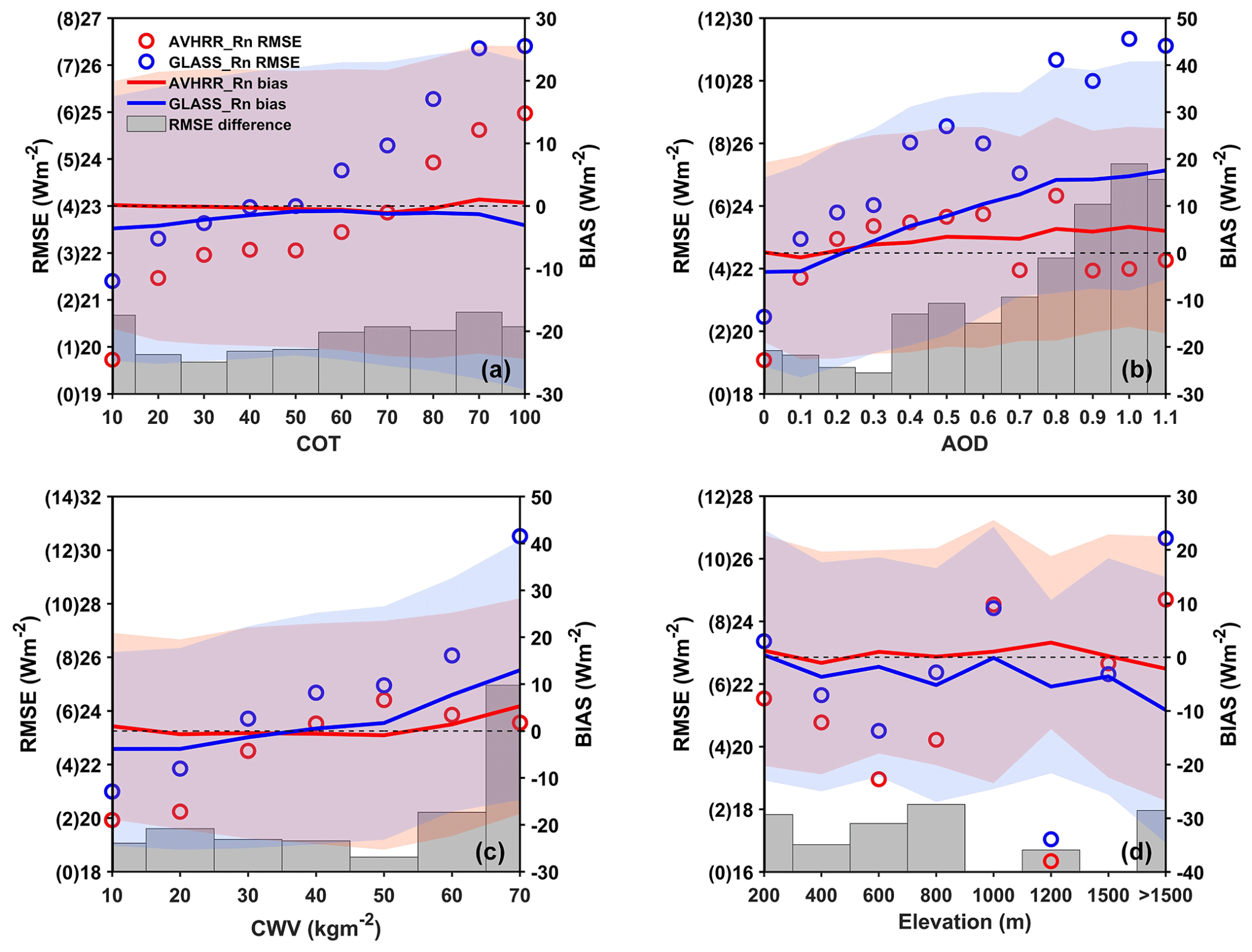
Figure 9Accuracy changes in AVHRR and GLASS Rn retrievals under different conditions for (a) cloud optical thickness (COT), (b) aerosol optical depth (AOD), (c) column water vapor (CWV), and (d) elevation. The values in parentheses on the left axis correspond to the RMSE differences denoted by bar charts. The shaded area shows the variance ranges of the biases.
4.3.3 Spatiotemporal analysis
The global-scale spatial distributions of mean AVHRR and GLASS surface Rn for January and July 2008 are displayed in Fig. 10. The missing values in the polar regions reflect the unavailability of valid data at the five bands in the case of the AVH02C1 product. The overall distribution of surface Rn for the two datasets is very similar, although slight differences exist in some regions, such as the TP region, the Sahara, and Greenland. AVHRR Rn retrievals are notably larger than the GLASS Rn retrievals in the TP region. Based on the results shown in Fig. 9d, greater confidence can be placed in the AVHRR Rn retrievals for high-elevation regions relative to GLASS Rn retrievals; however, the AVHRR Rn retrievals are lower in Greenland. Because few sites from the GC-Net and PROMICE networks were classified as reliable for the model training, the RCNN model has less knowledge about the spatiotemporal variations in Rn in Greenland compared to other regions. The validation results in Fig. 8 and Table 7 for the ice/snow surface cover type further confirm that the GLASS Rn product may offer a better performance in the Greenland region. Therefore, new algorithms and data are required for the polar regions to address this problem.
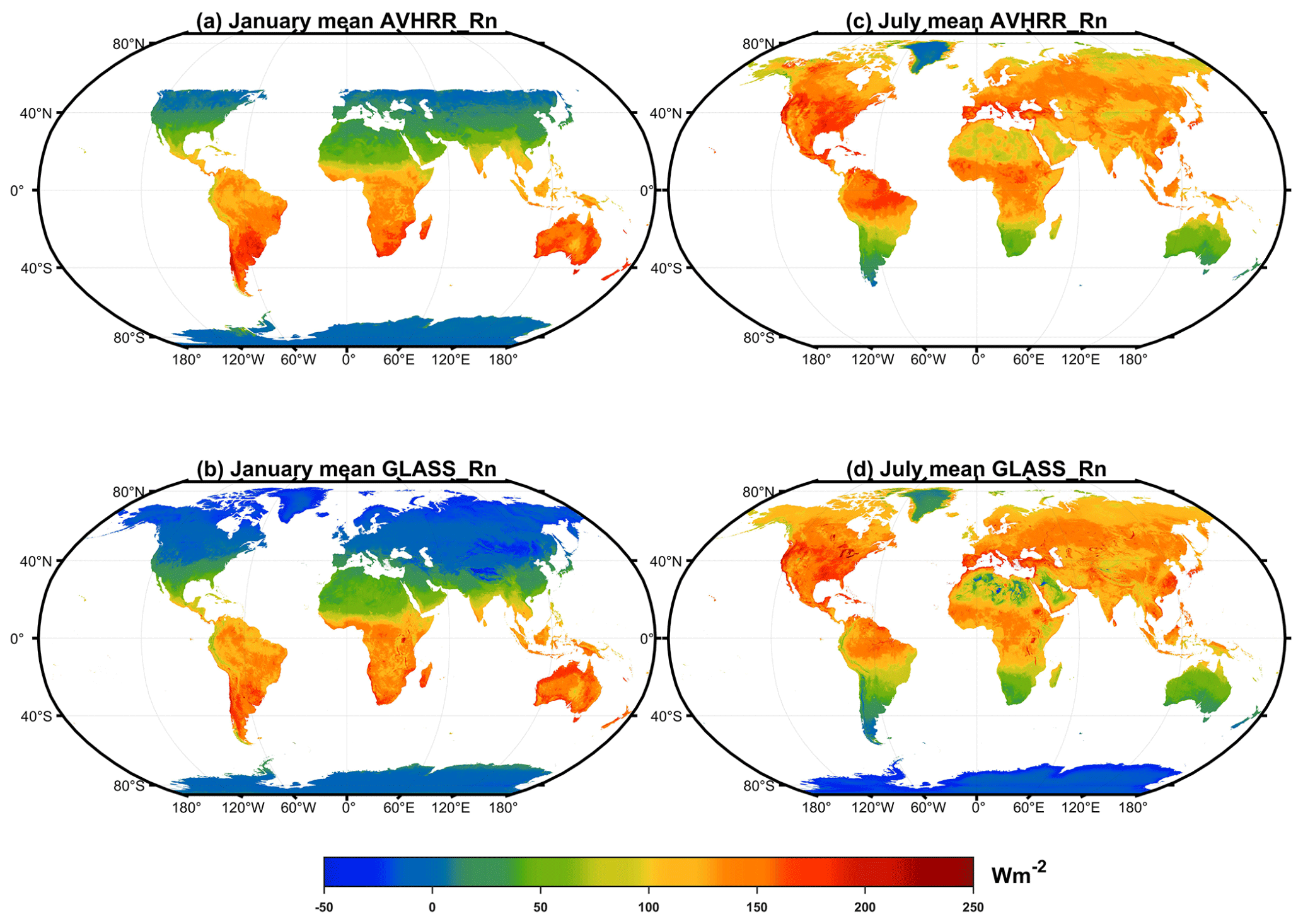
Figure 10Spatial distribution of monthly mean AVHRR and GLASS Rn retrievals in January (a, b) and July (c, d) 2008.
The spatiotemporal consistency of the AVHRR and GLASS daily Rn retrievals against COT was examined at a global scale in January and July 2008, respectively, as shown in Fig. 11. Overall, the spatial consistency is high for the two datasets. Specifically, in January, as the COT increases, the daily mean Rn values and the absolute differences between the two datasets also increase. As shown in Fig. 9a, when COT increases, the AVHRR Rn retrievals are more accurate. Thus we believe that the large discrepancies under high-COT conditions are mainly attributed to the uncertainty in GLASS Rn retrievals. In July, surface daily mean Rn remained relatively stable under different COT conditions, and the absolute differences between the two datasets also remain steady, with a mean absolute difference of about 20 W m−2.
Based on the previous analysis, spatially adjacent information is important for surface Rn estimation when COT values are large; however, if the cover of the entire cloud layer is small compared to the scale of the AVHRR footprint, the spatially adjacent effects will be significantly weakened in the inversion process, even if the corresponding COT is large. IPA-provided information includes the properties of the entire cloud layer. Figure S3 shows the spatial distribution of the monthly mean cloud cover fraction (CF) at the global scale in January and July and the corresponding differences in CFs (January − July). In January, the CFs are higher than in July over most land regions except in Central Africa, South Asia, Southern Australia, and Antarctica. However, most regions had smaller CFs in July. The differences in CFs for the two months are also marked; the positive differences demonstrate that more than 72 % of the land pixels had a higher CF in January than in July. The spatially adjacent effects induced by clouds are more significant on surface Rn in January than in July. Therefore, when large and thick cloud layers exist, such as in the polar regions, CNN is a better choice for surface Rn estimation, especially for downward longwave radiation (DLR) because the temperature of the cloud base, which is an essential variable in the parameterized calculation of DLR, is difficult to retrieve from multispectral remote sensing (Yang and Cheng, 2020).
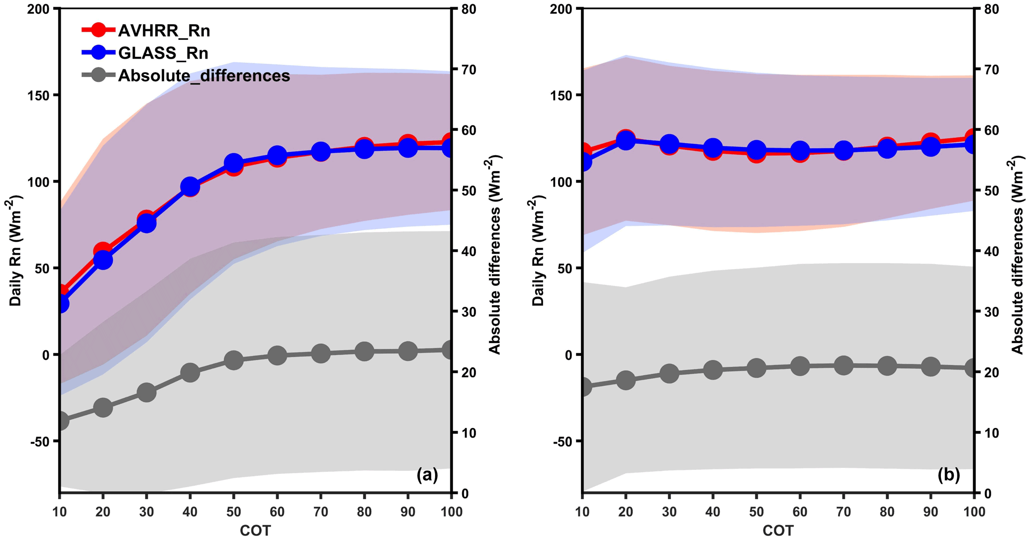
Figure 11Variations in the spatial and temporal consistency of AVHRR and GLASS daily Rn retrievals against cloud optical thickness (COT) in (a) January and (b) July 2008. The absolute difference is defined as |Rnavhrr−Rnglass|. The shading represents the variation range (standard deviation) of global daily AVHRR and GLASS Rn retrievals and their absolute differences.
4.3.4 Temporal analysis
To examine the temporal reliability of the generated AVHRR Rn dataset, a long-term analysis of surface Rn for the four datasets was carried out, the results of which are shown in Fig. 12. In view of missing values for the polar regions, we focused on surface Rn within the ±60∘ latitude region. Overall, the AVHRR Rn retrievals are highly consistent with MERRA-2 Rn values during the period of 1981 to 2019 as well as CERES and GLASS Rn retrievals after 2000. However, the MERRA-2 and CERES Rn values are generally higher than AVHRR Rn retrievals. Inter-comparison results illustrated that the CERES and MERRA-2 Rn values are overestimated against ground-based measurements. The GLASS Rn temporal profile is more consistently correlated with the AVHRR Rn retrievals.
Note that the LTDR project only uses afternoon satellite to generate the AVHRR product, which is to do with the high uncertainty in the atmospheric correction algorithm when applied to low-sun-elevation pixels present in morning satellites. Afternoon satellites include NOAA-7, NOAA-9, NOAA-11, NOAA-14, NOAA-16, NOAA-18, NOAA-19, and NOAA-20. The use of these satellites alone inevitably leads to small gaps in the data in exchange for a higher accuracy in the atmospheric correction. The time series is not fully complete and presents some observational gaps. Specifically, some large discrepancies occur, during some periods including 1994–1995, 1999–2000, 2007–2008, and 2018–2019. These periods correspond to the alternative update times of the NOAA-series satellites. For example, NOAA-11 was successfully succeeded by NOAA-14 from 1994 to 1995. Important gaps and noise were found in the images from March to September and empty data from September to December, due to NOAA-11 orbital degradation. NOAA-16 replaced NOAA-14 in 2000 for monitoring of the Earth's surface and atmosphere. During these periods of satellite replacement, the corresponding AVHRR data also contain large gaps. Similarly, NOAA-20 was launched on 18 November 2017, yet the quality of the AVHRR TOA observations from this platform was poor due to important gaps in the images and the presence of artifacts. This explains the abnormal temporal variations in the AVHRR Rn profile in these years shown in Fig. 12a. Therefore, effective multi-source data fusion algorithms and spatial gap-filling technology are urgently needed to improve the quality and coverage of the AVHRR Rn dataset.
The temporal variations in monthly Rn anomalies for the four datasets are shown in Fig. 12b. High temporal consistency exists between AVHRR Rn anomalies and the other three datasets. Specifically, the correlation coefficient for the AVHRR and MERRA-2 Rn anomalies for 1981–2019 is 0.952 and, for the period after 2000, is 0.957 and 0.956 for the AVHRR and CERES and for the AVHRR and GLASS Rn anomalies, respectively. Thus, the RCNN-derived AVHRR Rn dataset is temporally stable and reliable when the other three Rn datasets are used as a comparative baseline. In fact, the LTDR project has adapted a calibration method that can be consistently applied across the AVHRR instruments on board various NOAA satellites to account for sensor degradation (Vermote and Kaufman, 1995), which enables a temporally reliable Rn dataset to be produced. Following the approach, overall, our AVHRR Rn dataset is more accurate and shows reasonable spatiotemporal variations compared to the other three datasets. This dataset will play an important role in climate change study.
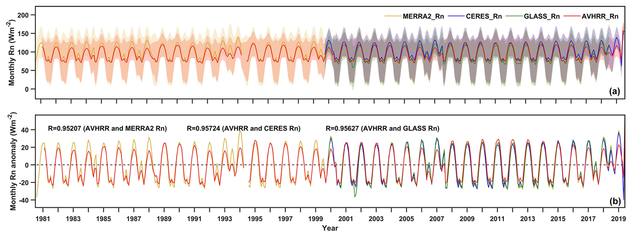
Figure 12Long-term temporal variation in (a) monthly average Rn and (b) monthly Rn anomalies for the AVHRR, CERES, GLASS, and MERRA-2 datasets. The shading represents the variation range (standard deviation) of the global monthly mean Rn.
5.1 Determination of an appropriate spatial scale
To provide appropriate AVHRR sub-image blocks containing sufficient information for the RCNN model to generate high-accuracy retrievals, the spatially adjacent effects on surface Rn under different valid spatial extents should be examined. For this, we used a simple multivariate linear regression (MLR) model (see Supplement for further details). The spatial sizes of the sub-images denoted as B3, …, B19 vary from 3 × 3 to 19 × 19, respectively, with an interval of 2 pixels. The true areas correspond to approximately 15 km × 15 km (B3) to 135 km × 135 km (B19) on the ground. The results are shown in Fig. 13. Overall, the average R increases from 0.61 to 0.708 and RMSE decreases from 50.12 to 46.17, respectively, for the MLR model. As the valid spatial extent increases, essential and complete spatial features are exposed and incorporated into the MLR model, which helps to continuously improve the model's retrieval accuracy. The spatial extent of B13 (approximately 65 km × 65 km) is the smallest size that exhibits convergent R and RMSE values, and the spatial extent at B15 reaches a more stable state for surface Rn estimations. This finding is in line with the results of Jiang et al. (2020b), showing that scale effects have a considerable impact on solar radiation retrieval accuracy and that distances of approximately 20 to 40 km from the central point (corresponding to areas of 40 km × 40 km to 80 km × 80 km) are the optimal spatial scale. In addition, previous studies (Hakuba et al., 2013; Huang et al., 2016) recommended a threshold distance of approximately 30 km, equal to a 13 × 13 grid region with a spatial resolution of 0.05∘, for shortwave radiation estimation. Therefore, a 15 × 15 grid area was selected for the input sub-images to generate AVHRR Rn retrievals.
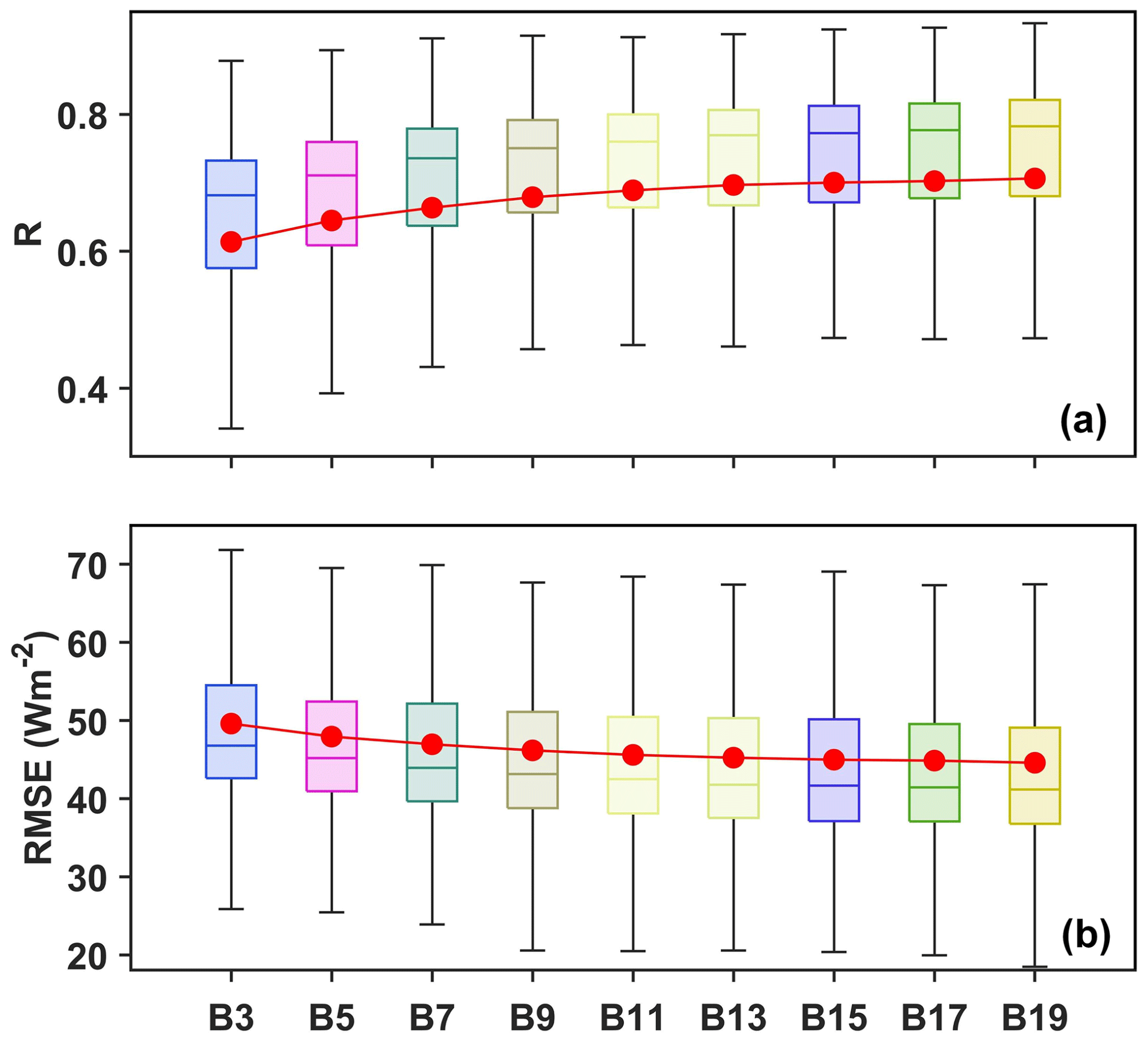
Figure 13Variations in (a) R and (b) RMSE indices for each spatial scale in the MLR model. The red lines in the subplots are the average curves of indices at the different spatial scales.
5.2 Role of daily mean MERRA-2 Rn
The RCNN model uses instantaneous satellite-sensed signals to directly estimate daily mean Rn retrievals. Though some previous studies (Chen et al., 2020; Wang et al., 2015a; Wang and Liang, 2017; Xu et al., 2020) directly estimated daily averaged surface radiation from instantaneous satellite observations, like MODIS, the idea is theoretically flawed because the AVHRR sensor only offers instantaneous “snapshots”, which cannot capture daily mean information about the diurnal cycles of the atmosphere and clouds. King et al. (2013) acknowledged that the frequency of cloud variations is high at different times and locations based on twin MODIS cloud products. In view of the wide satellite overpass times over a particular location, e.g., the equatorial crossing time generally ranges from 13:00 to 17:30 local time, representing different instantaneous atmospheric conditions for different AVHRR sensors, daily mean MERRA-2 Rn is incorporated into the input collection to provide daily mean information about the surface, atmosphere, and clouds for the RCNN model.
Figure 14 shows the effect of the daily mean MERRA-2 Rn on the final AVHRR Rn retrievals at different AVHRR overpass times in local time. The improved effect is slightly more significant during the afternoon than in the morning when more over-land clouds are present (King et al., 2013). This improvement is also more pronounced during the night. The AVHRR Rn retrievals can only be obtained when solar radiation is available (Fig. 10) because of the missing values in the AVH02C1 product; therefore, the results during the night are based on the validation results for high latitudes, which demonstrate that daily mean information about the diurnal cycles of the atmosphere and clouds is more important for daily surface radiation estimation at high latitudes than that at middle and low latitudes. Shupe et al. (2011) found annual cloud occurrence fractions are 58 %–83 % at the Arctic observatories, with a clear annual cycle wherein clouds are least frequent in the winter and most frequent in the late summer and autumn.
Additionally, MERRA-2 downward shortwave radiation (DSR) was used as a replacement for MERRA-2 Rn to test its contribution to daily mean surface Rn estimations when using instantaneous satellite data. The results presented in Fig. S4 show that the improved effect of daily MERRA-2 DSR is not comparable with that achieved using daily MERRA-2 Rn, and the former is closer to the results obtained when only instantaneous AVHRR observations are used. Therefore, MERRA-2 Rn is a meaningful input for the RCNN model. Moreover, the AVHRR Rn retrievals could also be further improved by using more accurate daily mean Rn data, such as GLASS Rn, or other parameters that accurately represent daily mean atmospheric and cloud variations.

Figure 14Effect of daily mean MERRA-2 Rn on AVHRR Rn retrievals at different satellite crossing times in local time over sites. The bars indicate RMSE, and lines indicate absolute biases. The shading shows the variation range of absolute bias.
5.3 Determination of a threshold for the ETC-derived correlation coefficient
The threshold for the ETC-derived correlation coefficient between in situ measurements and the unknown truth within the 5 km AVHRR grid in Eq. (2) affects the selection of reliable sites and the subsequent PSME process. A series of thresholds for the ETC-derived coefficients were considered, ranging from 0.2 to 0.9 with an interval of 0.1. In each case, the corresponding measurements from the selected reliable sites were fed into the RCNN model to train and subsequently generate AVHRR Rn retrievals. Then, the training and test accuracies of the RCNN were calculated over all of the reliable sites for comparison. Another important consideration is the representativeness of the RCNN for global Rn estimation given that the number of reliable training sites decreases with higher thresholds. Thus, the trained RCNN model was again evaluated at all sites, including reliable and unreliable sites, to examine the global representativeness. The number of reliable sites (training and test accuracies) and the associated global accuracy are presented in Fig. 15. As the threshold increased, the number of reliable sites decreased. The training and test relative RMSEs of the RCNN model showed a general decreasing trend, especially above a threshold of 0.5, which illustrates that the selection of reliable sites and the measurements from these sites have better representativeness for the AVHRR footprint scale using ETC. This helps address the spatial-scale mismatch issue and improve the accuracy of AVHRR retrievals at a 5 km resolution. In addition, a trade-off between the RCNN's fitting accuracy at the reliable sites and the global accuracy at all sites needs to be considered. Even when a threshold of 0.9 was used, the global accuracy of the RCNN was only slightly lower, which explains why this threshold was applied in Sect. 3.1.
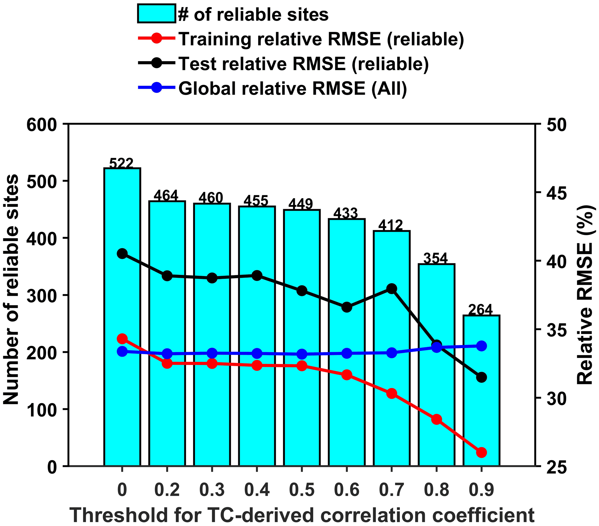
Figure 15Effect of extended triplet collocation (ETC)-derived correlation coefficients on the number of reliable sites and the corresponding RCNN's training, test, and global accuracies.
5.4 Orbital drift of the NOAA-series satellites
The orbital drift problem of the NOAA-series satellites has attracted the attention of users applying AVHRR-derived high-level remote sensing products, such as land surface temperature (LST) (Ma et al., 2020; Liu et al., 2019) and TOA albedo (Song et al., 2018). As shown in Fig. 16, the orbital drift makes the true equatorial crossing time (ECT) of the NOAA-series afternoon satellites range from 13:00 to 17:30 in the solar time system. Previous geophysical variable retrievals based on AVHRR data are instantaneous values at satellite overpass times, which need to be corrected to a specific time, such as LST at 14:30 and albedo at noon local time. However, the RCNN model uses instantaneous AVHRR TOA observations at different satellite overpass times to directly retrieve daily surface Rn estimates, which differs from previous studies.
Additionally, daily MERRA-2 Rn and instantaneous SZA values closely related to satellite transit times are taken as inputs; therefore, the RCNN model can automatically learn the relationships between instantaneous satellite data at different overpass times and corresponding daily surface Rn measurements. Moreover, the results of the long-term temporal analysis of the AVHRR Rn dataset provide more evidence to ensure that the quality of the long-term AVHRR daily Rn datasets is not affected by orbital drift. As such, orbital drift does not affect our long-term AVHRR Rn dataset.
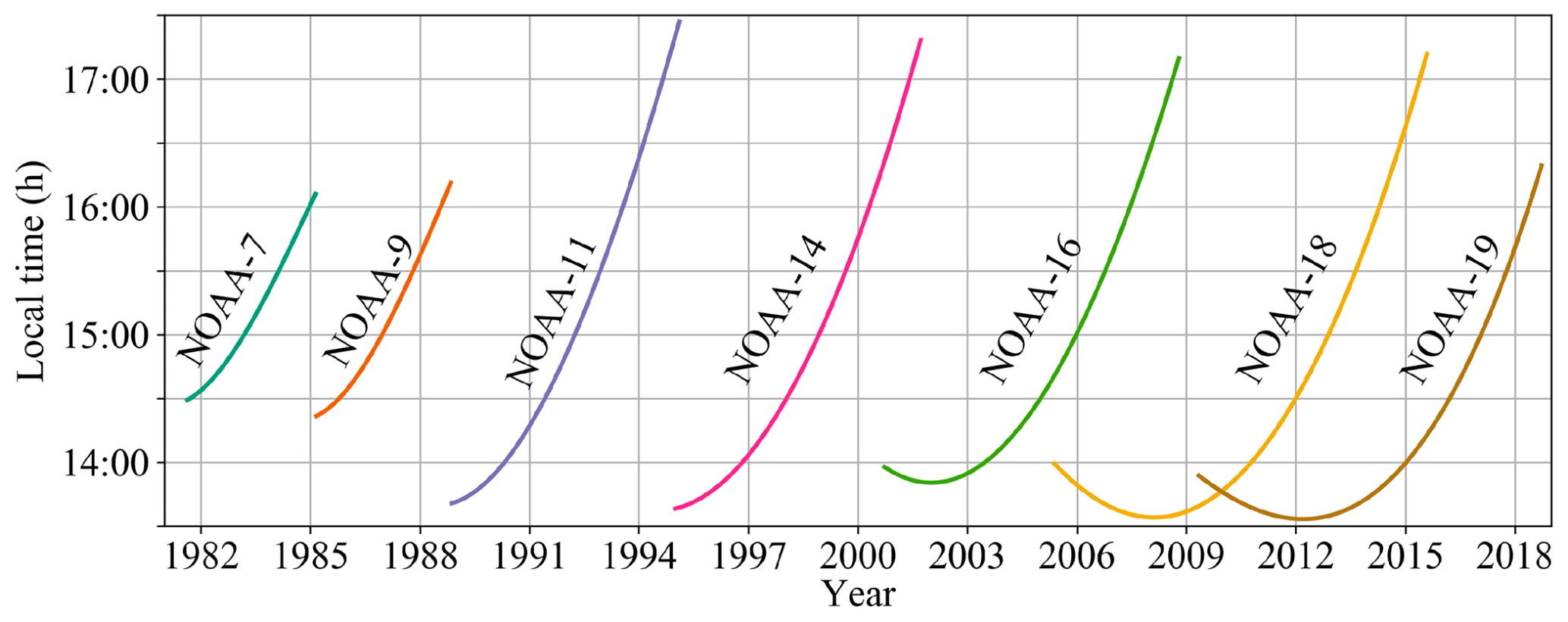
Figure 16Equatorial crossing time (ECT) for the National Oceanic and Atmospheric Administration (NOAA)-series afternoon satellites. Figure obtained from Liu et al. (2019).
Global surface Rn retrieved from NOAA AVHRR data from 1981 to 2019 are freely available at https://doi.org/10.5281/zenodo.5546316 (Xu et al., 2021).
The AVH02C1 product data were downloaded from the Level-1 and Atmosphere Archive & Distribution System Distributed Active Archive Center (https://ladsweb.modaps.eosdis.nasa.gov/, last access: 2 July 2021; Pedelty et al., 2007). The CERES-SYN product was downloaded from the CERES team (https://ceres.larc.nasa.gov/, last access: 2 July 2021; Doelling et al., 2016). The GLASS Rn product was provided by the GLASS team at http://www.glass.umd.edu/ (last access: 2 July 2021; Liang et al., 2021). MERRA-2 reanalysis was downloaded from the Global Modeling and Assimilation Office (https://gmao.gsfc.nasa.gov/, last access: 2 July 2021; Gelaro et al., 2017b). The download links of ground-based measurements from different observational networks are referenced in Jiang et al. (2018).
A long-term (1981–2019) global daily surface Rn product with a spatial resolution of 0.05∘ was generated from historical NOAA-series AVHRR data using an RCNN-based PSME method. The specific steps employed were as follows: (1) selecting reliable sites from all sites based on ETC to generate the sample dataset, (2) training and independent testing of the proposed RCNN model, (3) evaluating the AVHRR Rn retrievals against in situ measurements and performing inter-comparisons with three other Rn products (GLASS, CERES-SYN, and MERRA-2), and (4) generating and evaluating the long-term AVHRR Rn product.
ETC was first applied to select reliable sites to prepare a sample dataset with better spatial representativeness at the AVHRR footprint scale (i.e., 5 km). In total, 262 sites were classified as reliable sites from a total of 522 sites and used as a sample dataset for the RCNN model. The proportions of the selected reliable sites representing cropland and grassland surfaces were highest (∼ 66 % and ∼ 62 %, respectively), while those representing ice/snow surface were lowest (∼ 14 %). The sample dataset from the 262 sites ensured that the trained RCNN model had both a good fitting accuracy for the reliable sites and global accuracy across all sites.
A simple MLR model was used to examine the spatially adjacent effects on surface Rn estimation, and a spatial extent of 15 × 15 pixels (75 km × 75 km) was then determined as the input size of the RCNN to provide sufficient spatial information. Based on 10-fold CV, the trained RCNN model achieved an R2 of 0.90, with an RMSE of 20.84 W m−2 (25.97 %) and a bias of −0.45 W m−2 (−0.57 %); the corresponding independent validation values were 0.84, 26.77 W m−2 (31.54 %), and 1.16 W m−2 (1.37 %), respectively, at the reliable sites. These results demonstrate the overall ability of the RCNN model to accurately predict surface Rn.
The results of an inter-comparison between the AVHRR Rn retrievals and three other products illustrated that our retrievals show a better accuracy against in situ measurements, with an R2 of 0.90, RMSE of 21.08 W m−2 (26.22 %), and bias of −0.38 W m−2 (−0.47 %) at the reliable sites, and an R2 of 0.85, RMSE of 26.74 W m−2 (35.70 %), and bias of 1.20 W m−2 (1.60 %) across all sites. At the same time, the AVHRR Rn retrievals show better performance for different observational networks and surface cover types, except for the snow/ice surface cover. Under different elevations and atmospheric conditions, the AVHRR Rn retrievals performed better than the GLASS Rn equivalent, especially in the presence of thick clouds and hazy atmospheric conditions because of the integration of spatially adjacent information into the inversion process in the RCNN model. In addition, the spatiotemporal variation in the AVHRR Rn retrievals is similar to that of the GLASS Rn values, demonstrating the ability of the RCNN model to generate a long-term global Rn product.
The long-term global Rn dataset generated by the RCNN model displays high accuracy and reasonable spatiotemporal variation at the global scale, which is suited to many applications including, for example, studies to understand the radiation budget and global climate change. Besides, compared to current satellite-derived Rn products, e.g., CERES-SYN and GLASS (2000–present), a longer record (1981–2019) of the AVHRR Rn dataset shows its value in climate change studies. However, further research is needed to solve some problems to further improve the data quality of the AVHRR Rn dataset. First, new algorithms and satellite data are needed to estimate surface Rn in the polar regions, such as MODIS data (Chen et al., 2020). Second, an effective data gap-filling method or multi-source data fusion algorithm is required to fill the data gaps over land, especially during periods of satellite replacement work. Third, coupled with spatially adjacent information, real-time temporal information or historical information should be incorporated to further improve the accuracy of the Rn retrievals.
As a type of machine learning, deep learning involves using data-driven models to find potential relationships and patterns and offers high adaptability to training data sample inputs. The predictive ability of a data-driven model completely depends on the limitations of the training dataset and, in the case of Rn, the ability of the model to accurately portray spatiotemporal dynamics in areas where the availability of training data is relatively poor, such as for AVHRR Rn retrievals for ice-/snow-covered surfaces. To address this problem, more physical knowledge is needed to fully utilize data-driven modeling to estimate surface Rn under different atmospheric and surface conditions. In particular, more attention should be paid to understanding inherent physical processes in addition to obtaining optimal estimation by coupling physical process models with the versatility of data-driven machine learning (Reichstein et al., 2019).
The supplement related to this article is available online at: https://doi.org/10.5194/essd-14-2315-2022-supplement.
JX and SL contributed to the design of this study and developed the overall methodology. JX and BJ collected and preprocessed the data. JX carried out the experiment and produced the product. JX wrote the first draft. All authors revised the manuscript.
The contact author has declared that neither they nor their co-authors have any competing interests.
Publisher's note: Copernicus Publications remains neutral with regard to jurisdictional claims in published maps and institutional affiliations.
The authors would like to thank the LTDR project for providing the AVH02C1 product, CERES team for offering the CERES-SYN flux product, NASA team for the MERRA-2 product, and GLASS team for the GLASS Rn product. We express our gratitude to each observation network project for providing ground-based radiation measurements, including ARM, BSRN, AsiaFlux, GC-Net, the global FLUXNET, PROMICE and other networks/programs.
This work was supported by the Chinese Grand Research Program on Climate Change and Response (project 2016YFA0600103) and the National Natural Science Foundation of China (grant 41971291).
This paper was edited by Christof Lorenz and reviewed by two anonymous referees.
Augustine, J. A., DeLuisi, J. J., and Long, C. N.: SURFRAD – A national surface radiation budget network for atmospheric research, B. Am. Meteorol. Soc., 81, 2341–2358, 2000.
Ball, J. E., Anderson, D. T., and Chan, C. S.: Comprehensive survey of deep learning in remote sensing: theories, tools, and challenges for the community, J. Appl. Remote Sens., 11, 042609, https://doi.org/10.1117/1.JRS.11.042609, 2017.
Barker, H. W. and Li, Z.: Interpreting shortwave albedo-transmittance plots: True or apparent anomalous absorption?, Geophys. Res. Lett., 24, 2023–2026, 1997.
Betts, A. K., Zhao, M., Dirmeyer, P., and Beljaars, A.: Comparison of ERA40 and NCEP/DOE near-surface data sets with other ISLSCP-II data sets, J. Geophys. Res.-Atmos., 111, D22S04, https://doi.org/10.1029/2006JD007174, 2006.
Bisht, G. and Bras, R. L.: Estimation of net radiation from the MODIS data under all sky conditions: Southern Great Plains case study, Remote Sens. Environ., 114, 1522–1534, 2010.
Bisht, G., Venturini, V., Islam, S., and Jiang, L.: Estimation of the net radiation using MODIS (Moderate Resolution Imaging Spectroradiometer) data for clear sky days, Remote Sens. Environ., 97, 52–67, 2005.
Box, J. E. and Rinke, A.: Evaluation of Greenland ice sheet surface climate in the HIRHAM regional climate model using automatic weather station data, J. Climate, 16, 1302–1319, 2003.
Chen, F., Crow, W. T., Colliander, A., Cosh, M. H., Jackson, T. J., Bindlish, R., Reichle, R. H., Chan, S. K., Bosch, D. D., Starks, P. J., Goodrich, D. C., and Seyfried, M. S.: Application of Triple Collocation in Ground-Based Validation of Soil Moisture Active/Passive (SMAP) Level 2 Data Products, IEEE J. Sel. Top. Appl., 10, 489–502, https://doi.org/10.1109/JSTARS.2016.2569998, 2017.
Chen, J., He, T., Jiang, B., and Liang, S.: Estimation of all-sky all-wave daily net radiation at high latitudes from MODIS data, Remote Sens. Environ., 245, 111842, https://doi.org/10.1016/j.rse.2020.111842, 2020.
Cheng, J. and Liang, S.: Global estimates for high-spatial-resolution clear-sky land surface upwelling longwave radiation from MODIS data, IEEE T. Geosci. Remote, 54, 4115–4129, 2016.
Cheng, J., Liang, S., Wang, W., and Guo, Y.: An efficient hybrid method for estimating clear-sky surface downward longwave radiation from MODIS data, J. Geophys. Res.-Atmos., 122, 2616–2630, https://doi.org/10.1002/2016JD026250, 2017.
Crow, W. T., Berg, A. A., Cosh, M. H., Loew, A., Mohanty, B. P., Panciera, R., de Rosnay, P., Ryu, D., and Walker, J. P.: Upscaling sparse ground-based soil moisture observations for the validation of coarse-resolution satellite soil moisture products, Rev. Geophys., 50, RG2002, https://doi.org/10.1029/2011RG000372, 2012.
Delgado-Bonal, A., Marshak, A., Yang, Y., and Holdaway, D.: Analyzing changes in the complexity of climate in the last four decades using MERRA-2 radiation data, Sci. Rep., 10, 922, https://doi.org/10.1038/s41598-020-57917-8, 2020.
Doelling, D. R., Loeb, N. G., Keyes, D. F., Nordeen, M. L., Morstad, D., Nguyen, C., Wielicki, B. A., Young, D. F., and Sun, M.: Geostationary Enhanced Temporal Interpolation for CERES Flux Products, J. Atmos. Ocean. Tech., 30, 1072–1090, https://doi.org/10.1175/jtech-d-12-00136.1, 2013.
Doelling, D. R., Sun, M., Nguyen, L. T., Nordeen, M. L., Haney, C. O., Keyes, D. F., and Mlynczak, P. E.: Advances in geostationary-derived longwave fluxes for the CERES synoptic (SYN1deg) product, J. Atmos. Ocean. Tech., 33, 503–521, 2016.
Draper, C., Reichle, R., de Jeu, R., Naeimi, V., Parinussa, R., and Wagner, W.: Estimating root mean square errors in remotely sensed soil moisture over continental scale domains, Remote Sens. Environ., 137, 288–298, 2013.
Fillmore, D., Rutan, D., Kato, S., Rose, F., and Caldwell, T.: Evaluation of aerosol optical depths and clear-sky radiative fluxes of the CERES Edition 4.1 SYN1deg data product, Atmos. Chem. Phys. Discuss. [preprint], https://doi.org/10.5194/acp-2021-283, in review, 2021.
Gelaro, R., McCarty, W., Suárez, M. J., Todling, R., Molod, A., Takacs, L., Randles, C. A., Darmenov, A., Bosilovich, M. G., and Reichle, R.: The modern-era retrospective analysis for research and applications, version 2 (MERRA-2), J. Climate, 30, 5419–5454, 2017a.
Gelaro, R., McCarty, W., Suárez, M. J., Todling, R., Molod, A., Takacs, L., Randles, C. A., Darmenov, A., Bosilovich, M. G., Reichle, R., Wargan, K., Coy, L., Cullather, R., Draper, C., Akella, S., Buchard, V., Conaty, A., da Silva, A. M., Gu, W., Kim, G.-K., Koster, R., Lucchesi, R., Merkova, D., Nielsen, J. E., Partyka, G., Pawson, S., Putman, W., Rienecker, M., Schubert, S. D., Sienkiewicz, M., and Zhao, B.: The Modern-Era Retrospective Analysis for Research and Applications, Version 2 (MERRA-2), J. Climate, 30, 5419–5454, https://doi.org/10.1175/jcli-d-16-0758.1, 2017b.
Géron, A.: Hands-on machine learning with Scikit-Learn, Keras, and TensorFlow: Concepts, tools, and techniques to build intelligent systems, O'Reilly Media, Inc., Sebastopol, CA, USA, 2019.
Gruber, A., Su, C.-H., Zwieback, S., Crow, W., Dorigo, W., and Wagner, W.: Recent advances in (soil moisture) triple collocation analysis, Int. J. Appl. Earth Obs., 45, 200–211, 2016.
Guo, X., Yao, Y., Zhang, Y., Lin, Y., and Bei, X.: Discrepancies in the Simulated Global Terrestrial Latent Heat Flux from GLASS and MERRA-2 Surface Net Radiation Products, Remote Sensing, 12, 2763, https://doi.org/10.3390/rs12172763, 2020.
Hakuba, M. Z., Folini, D., Sanchez-Lorenzo, A., and Wild, M.: Spatial representativeness of ground-based solar radiation measurements, J. Geophys. Res.-Atmos., 118, 8585–8597, 2013.
Hao, D., Wen, J., Xiao, Q., Wu, S., Lin, X., Dou, B., You, D., and Tang, Y.: Simulation and analysis of the topographic effects on snow-free albedo over rugged terrain, Remote Sensing, 10, 278, https://doi.org/10.1016/j.rse.2019.111320, 2018.
Hao, D., Asrar, G., Zeng, Y., Zhu, Q., Wen, J., Xiao, Q., and Chen, M.: Estimating hourly land surface downward shortwave and photosynthetically active radiation from DSCOVR/EPIC observations, Remote Sens. Environ., 232, 111320, https://doi.org/10.3390/rs10020278, 2019.
He, K., Zhang, X., Ren, S., and Sun, J.: Deep Residual Learning for Image Recognition, 2016 IEEE Conference on Computer Vision and Pattern Recognition (CVPR), 770–778, https://doi.org/10.1109/CVPR.2016.90, 2016.
He, T., Liang, S., Wang, D., Shi, Q., and Goulden, M. L.: Estimation of high-resolution land surface net shortwave radiation from AVIRIS data: Algorithm development and preliminary results, Remote Sens. Environ., 167, 20–30, 2015.
Hersbach, H., Bell, B., Berrisford, P., Hirahara, S., Horányi, A., Muñoz-Sabater, J., Nicolas, J., Peubey, C., Radu, R., and Schepers, D.: The ERA5 global reanalysis, Q. J. Roy. Meteor. Soc., 146, 1999–2049, 2020.
Huang, G., Ma, M., Liang, S., Liu, S., and Li, X.: A LUT-based approach to estimate surface solar irradiance by combining MODIS and MTSAT data, J. Geophys. Res-Atmos., 116, 6255–6265, https://doi.org/10.1029/2011JD016120, 2011.
Huang, G., Li, X., Huang, C., Liu, S., Ma, Y., and Chen, H.: Representativeness errors of point-scale ground-based solar radiation measurements in the validation of remote sensing products, Remote Sens. Environ., 181, 198–206, 2016.
Huang, G., Li, X., Lu, N., Wang, X., and He, T.: A General Parameterization Scheme for the Estimation of Incident Photosynthetically Active Radiation Under Cloudy Skies, IEEE T. Geosci. Remote, 116, D22201, https://doi.org/10.1029/2011JD016120, 2020.
Jia, A., Jiang, B., Liang, S., Zhang, X., and Ma, H.: Validation and spatiotemporal analysis of CERES surface net radiation product, Remote Sensing, 8, 90, https://doi.org/10.3390/rs8020090, 2016.
Jia, A., Liang, S., Jiang, B., Zhang, X., and Wang, G.: Comprehensive assessment of global surface net radiation products and uncertainty analysis, J. Geophys. Res.-Atmos., 123, 1970–1989, 2018.
Jiang, B., Zhang, Y., Liang, S., Zhang, X., and Xiao, Z.: Surface Daytime Net Radiation Estimation Using Artificial Neural Networks, Remote Sensing, 6, 11031–11050, 2014.
Jiang, B., Zhang, Y., Liang, S., Wohlfahrt, G., Arain, A., Cescatti, A., Georgiadis, T., Jia, K., Kiely, G., Lund, M., Montagnani, L., Magliulo, V., Ortiz, P. S., Oechel, W., Vaccari, F. P., Yao, Y., and Zhang, X.: Empirical estimation of daytime net radiation from shortwave radiation and ancillary information, Agr. Forest Meteorol., 211–212, 23–36, 2015.
Jiang, B., Liang, S., Ma, H., Zhang, X., Xiao, Z., Zhao, X., Jia, K., Yao, Y., and Jia, A.: GLASS daytime all-wave net radiation product: Algorithm development and preliminary validation, Remote Sensing, 8, 222, https://doi.org/10.3390/rs8030222, 2016.
Jiang, B., Liang, S., Jia, A., Xu, J., Zhang, X., Xiao, Z., Zhao, X., Jia, K., and Yao, Y.: Validation of the Surface Daytime Net Radiation Product From Version 4.0 GLASS Product Suite, IEEE Geosci. Remote Sens. Lett., 16, 509–513, 2018.
Jiang, H., Lu, N., Qin, J., and Yao, L.: Surface global and diffuse solar radiation over China acquired from geostationary Multi-functional Transport Satellite data, Earth Syst. Sci. Data Discuss. [preprint], https://doi.org/10.5194/essd-2019-209, 2019a.
Jiang, H., Lu, N., Qin, J., Tang, W., and Yao, L.: A deep learning algorithm to estimate hourly global solar radiation from geostationary satellite data, Renew. Sust.e Energ. Rev., 114, 109327, https://doi.org/10.1016/j.rser.2019.109327, 2019b.
Jiang, H., Lu, N., Qin, J., and Yao, L.: Hourly 5-km surface total and diffuse solar radiation in China, 2007–2018, Sci. Data, 7, 311, https://doi.org/10.1038/s41597-020-00654-4, 2020a.
Jiang, H., Lu, N., Huang, G., Yao, L., Qin, J., and Liu, H.: Spatial scale effects on retrieval accuracy of surface solar radiation using satellite data, Appl. Energ., 270, 115178, https://doi.org/10.1016/j.apenergy.2020.115178, 2020b.
Jiao, Z., Yan, G., Zhao, J., Wang, T., and Chen, L.: Estimation of surface upward longwave radiation from MODIS and VIIRS clear-sky data in the Tibetan Plateau, Remote Sens. Environ., 162, 221–237, 2015.
Jung, M., Koirala, S., Weber, U., Ichii, K., Gans, F., Camps-Valls, G., Papale, D., Schwalm, C., Tramontana, G., and Reichstein, M.: The FLUXCOM ensemble of global land-atmosphere energy fluxes, Sci. Data, 6, 1–14, 2019a.
Jung, M., Koirala, S., Weber, U., Ichii, K., Gans, F., Camps-Valls, G., Papale, D., Schwalm, C., Tramontana, G., and Reichstein, M.: The FLUXCOM ensemble of global land-atmosphere energy fluxes, Sci. Data, 6, 74, https://doi.org/10.1038/s41597-019-0076-8, 2019b.
Kanamitsu, M., Ebisuzaki, W., Woollen, J., Yang, S.-K., Hnilo, J., Fiorino, M., and Potter, G.: Ncep–doe amip-ii reanalysis (r-2), B. Am. Meteorol. Soc., 83, 1631–1644, 2002.
King, M. D., Platnick, S., Menzel, W. P., Ackerman, S. A., and Hubanks, P. A.: Spatial and temporal distribution of clouds observed by MODIS onboard the Terra and Aqua satellites, IEEE T. Geosci. Remote, 51, 3826–3852, 2013.
Kobayashi, S., Ota, Y., Harada, Y., Ebita, A., Moriya, M., Onoda, H., Onogi, K., Kamahori, H., Kobayashi, C., and Endo, H.: The JRA-55 reanalysis: General specifications and basic characteristics, J. Meteorol. Soc. Jpn. Ser. II, 93, 5–48, 2015.
Letu, H., Shi, J., Li, M., Wang, T., Shang, H., Lei, Y., Ji, D., Wen, J., Yang, K., and Chen, L.: A review of the estimation of downward surface shortwave radiation based on satellite data: Methods, progress and problems, Science China Earth Sciences, 63, 774–789, https://doi.org/10.1007/s11430-019-9589-0, 2020.
Li, T. and Cheng, X.: Estimating daily full-coverage surface ozone concentration using satellite observations and a spatiotemporally embedded deep learning approach, Int. J. Appl. Earth Obs., 101, 102356, https://doi.org/10.1016/j.jag.2021.102356, 2021.
Li, T., Wang, Y., and Yuan, Q.: Remote Sensing Estimation of Regional NO2 via Space-Time Neural Networks, Remote Sensing, 12, 2514, https://doi.org/10.3390/rs12162514, 2020a.
Li, T., Shen, H., Yuan, Q., and Zhang, L.: Geographically and temporally weighted neural networks for satellite-based mapping of ground-level PM2.5, ISPRS J. Photogramm, 167, 178–188, 2020b.
Liang, S., Wang, K., Zhang, X., and Wild, M.: Review on estimation of land surface radiation and energy budgets from ground measurement, remote sensing and model simulations, IEEE J. Sel. Top. Appl., 3, 225–240, 2010.
Liang, S., Wang, D., He, T., and Yu, Y.: Remote sensing of earth's energy budget: synthesis and review, Int. J. Digit. Earth, 12, 737–780, 2019.
Liang, S., Cheng, J., Jia, K., Jiang, B., Liu, Q., Xiao, Z., Yao, Y., Yuan, W., Zhang, X., and Zhao, X.: The Global LAnd Surface Satellite (GLASS) product suite, B. Am. Meteorol. Soc., 102, E323–E337, https://doi.org/10.1175/bams-d-18-0341.1, 2020.
Liang, S., Cheng, J., Jia, K., Jiang, B., Liu, Q., Xiao, Z., Yao, Y., Yuan, W., Zhang, X., Zhao, X., and Zhou, J.: The Global Land Surface Satellite (GLASS) Product Suite, B. Am. Meteorol. Soc., 102, E323–E337, https://doi.org/10.1175/bams-d-18-0341.1, 2021.
Liu, X., Tang, B.-H., Yan, G., Li, Z.-L., and Liang, S.: Retrieval of global orbit drift corrected land surface temperature from long-term AVHRR data, Remote Sensing, 11, 2843, https://doi.org/10.3390/rs11232843, 2019.
Loeb, N. G., Doelling, D. R., Wang, H., Su, W., Nguyen, C., Corbett, J. G., Liang, L., Mitrescu, C., Rose, F. G., and Kato, S.: Clouds and the earth's radiant energy system (CERES) energy balanced and filled (EBAF) top-of-atmosphere (TOA) edition-4.0 data product, J. Climate, 31, 895–918, 2018.
Lu, N., Qin, J., Yang, K., and Sun, J.: A simple and efficient algorithm to estimate daily global solar radiation from geostationary satellite data, Energy, 36, 3179–3188, 2011.
Ma, J., Zhou, J., Göttsche, F.-M., Liang, S., Wang, S., and Li, M.: A global long-term (1981–2000) land surface temperature product for NOAA AVHRR, Earth Syst. Sci. Data, 12, 3247–3268, https://doi.org/10.5194/essd-12-3247-2020, 2020.
McColl, K. A., Vogelzang, J., Konings, A. G., Entekhabi, D., Piles, M., and Stoffelen, A.: Extended triple collocation: Estimating errors and correlation coefficients with respect to an unknown target, Geophys. Res. Lett., 41, 6229–6236, 2014.
Ohmura, A., Dutton, E. G., Forgan, B., Fröhlich, C., Gilgen, H., Hegner, H., Heimo, A., König-Langlo, G., McArthur, B., and Müller, G.: Baseline Surface Radiation Network (BSRN/WCRP): New precision radiometry for climate research, B. Am. Meteorol. Soc., 79, 2115–2136, 1998.
Pedelty, J., Devadiga, S., Masuoka, E., Brown, M., Pinzon, J., Tucker, C., Vermote, E., Prince, S., Nagol, J., Justice, C., Roy, D., Junchang, J., Schaaf, C., Jicheng, L., Privette, J., and Pinheiro, A.: Generating a Long-term Land Data Record from the AVHRR and MODIS Instruments, 2007 IEEE International Geoscience and Remote Sensing Symposium, 23–28 July 2007, 1021–1025, https://doi.org/10.1109/IGARSS.2007.4422974, 2007.
Philipona, R., Fröhlich, C., Dehne, K., DeLuisi, J., Augustine, J., Dutton, E., Nelson, D., Forgan, B., Novotny, P., and Hickey, J.: The Baseline Surface Radiation Network pyrgeometer round-robin calibration experiment, J. Atmos. Ocean. Tech., 15, 687–696, 1998.
Pinker, R. and Laszlo, I.: Modeling surface solar irradiance for satellite applications on a global scale, J. Appl. Meteorol. Clim., 31, 194–211, 1992.
Qin, J., Yang, K., Liang, S., and Tang, W.: Estimation of Daily Mean Photosynthetically Active Radiation under All-Sky Conditions Based on Relative Sunshine Data, J. Appl. Meteorol. Clim.gy, 51, 150–160, 2012.
Reichstein, M., Camps-Valls, G., Stevens, B., Jung, M., Denzler, J., and Carvalhais, N.: Deep learning and process understanding for data-driven Earth system science, Nature, 566, 195–204, 2019.
Román, M. O., Schaaf, C. B., Woodcock, C. E., Strahler, A. H., Yang, X., Braswell, R. H., Curtis, P. S., Davis, K. J., Dragoni, D., and Goulden, M. L.: The MODIS (Collection V005) BRDF/albedo product: Assessment of spatial representativeness over forested landscapes, Remote Sens. Environ., 113, 2476–2498, 2009.
Romanuke, V.: Appropriate Number and Allocation of RELUS in Convolutional Neural Networks. Research Bulletin of the National Technical University of Ukraine Kyiv Politechnic Institute, 69–78, https://doi.org/10.20535/1810-0546.2017.1.88156, 2017.
Rossow, W. and Zhang, Y. C.: Calculation of surface and top of atmosphere radiative fluxes from physical quantities based on ISCCP data sets: 2. Validation and first results, J. Geophys. Res.-Atmos., 100, 1167–1197, 1995.
Saha, S., Moorthi, S., Pan, H.-L., Wu, X., Wang, J., Nadiga, S., Tripp, P., Kistler, R., Woollen, J., and Behringer, D.: The NCEP climate forecast system reanalysis, B. Am. Meteor. Soc., 91, 1015–1058, 2010.
Sellers, P., Dickinson, R., Randall, D., Betts, A., Hall, F., Berry, J., Collatz, G., Denning, A., Mooney, H., and Nobre, C.: Modeling the exchanges of energy, water, and carbon between continents and the atmosphere, Science, 275, 502–509, 1997.
Shupe, M. D., Walden, V. P., Eloranta, E., Uttal, T., Campbell, J. R., Starkweather, S. M., and Shiobara, M.: Clouds at Arctic atmospheric observatories. Part I: Occurrence and macrophysical properties, J. Appl. Meteorol. Clim., 50, 626–644, 2011.
Song, Z., Liang, S., Wang, D., Zhou, Y., and Jia, A.: Long-term record of top-of-atmosphere albedo over land generated from AVHRR data, Remote Sens. Environ., 211, 71–88, 2018.
Stackhouse Jr., P., Gupta, S., Cox, S., Chiacchio, M., and Mikovitz, J.: The WCRP/GEWEX surface radiation budget project release 2: An assessment of surface fluxes at 1 degree resolution, in: IRS 2000: Current problems in atmospheric radiation, edited by: Smith, W. L. and Timofeyev, Y. M., International Radiation Symposium, St. Petersburg, Russia (2000), 24–29, 2000.
Steffen, K. and Box, J.: Surface climatology of the Greenland ice sheet: Greenland Climate Network 1995–1999, J. Geophys. Res.-Atmos., 106, 33951–33964, 2001.
Stoffelen, A.: Toward the true near-surface wind speed: Error modeling and calibration using triple collocation, J. Geophys. Res.-Oceans, 103, 7755–7766, 1998.
Stokes, G. M. and Schwartz, S. E.: The Atmospheric Radiation Measurement (ARM) Program: Programmatic background and design of the cloud and radiation test bed, B. Am. Meteor. Soc., 75, 1201–1222, 1994.
Tang, W., Yang, K., Qin, J., and Min, M.: Development of a 50-year daily surface solar radiation dataset over China, Science China Earth Sciences, 56, 1555–1565, 2013.
Tang, W., Qin, J., Yang, K., Niu, X., Min, M., and Liang, S.: An efficient algorithm for calculating photosynthetically active radiation with MODIS products, Remote Sens. Enviro., 194, 146–154, 2017.
Tang, W., Yang, K., Qin, J., Li, X., and Niu, X.: A 16-year dataset (2000–2015) of high-resolution (3 h, 10 km) global surface solar radiation, Earth Syst. Sci. Data, 11, 1905–1915, https://doi.org/10.5194/essd-11-1905-2019, 2019.
Tang, W.-J., Yang, K., Qin, J., Cheng, C. C. K., and He, J.: Solar radiation trend across China in recent decades: a revisit with quality-controlled data, Atmos. Chem. Phys., 11, 393–406, https://doi.org/10.5194/acp-11-393-2011, 2011.
Verma, M., Fisher, J. B., Mallick, K., Ryu, Y., Kobayashi, H., Guillaume, A., Moore, G., Ramakrishnan, L., Hendrix, V., and Wolf, S.: Global surface net-radiation at 5 km from MODIS Terra, Remote Sensing, 8, 739, https://doi.org/10.3390/rs8090739, 2016.
Vermote, E. and Kaufman, Y.: Absolute calibration of AVHRR visible and near-infrared channels using ocean and cloud views, Int. J. Remote Sens., 16, 2317–2340, 1995.
Wang, B., Yuan, Q., Yang, Q., Zhu, L., Li, T., and Zhang, L.: Estimate hourly PM2.5 concentrations from Himawari-8 TOA reflectance directly using Geo-intelligent long short-term memory network, Environ. Pollut., 271, 116327, https://doi.org/10.1016/j.envpol.2020.116327, 2020.
Wang, D. and Liang, S.: Estimating top-of-atmosphere daily reflected shortwave radiation flux over land from MODIS data, IEEE T. Geosci. Remote, 55, 4022–4031, 2017.
Wang, D., Liang, S., He, T., and Shi, Q.: Estimation of daily surface shortwave net radiation from the combined MODIS data, IEEE T. Geosci. Remote, 53, 5519–5529, 2015a.
Wang, D., Liang, S., He, T., and Shi, Q.: Estimating clear-sky all-wave net radiation from combined visible and shortwave infrared (VSWIR) and thermal infrared (TIR) remote sensing data, Remote Sens. Environ., 167, 31–39, 2015b.
Wang, D., Liang, S., Zhang, Y., Gao, X., and Jia, A.: A New Set of MODIS Land Products (MCD18): Downward Shortwave Radiation and Photosynthetically Active Radiation, Remote Sensing, 12, 168, https://doi.org/10.3390/rs12010168, 2020.
Wang, K. and Dickinson, R. E.: Global atmospheric downward longwave radiation at the surface from ground-based observations, satellite retrievals, and reanalyses, Rev. Geophys., 51, 150–185, 2013.
Wang, K. and Liang, S.: Estimation of daytime net radiation from shortwave radiation measurements and meteorological observations, J. Appl. Meteorol. Clim., 48, 634–643, 2009.
Wang, Y., Jiang, B., Liang, S., Wang, D., He, T., Wang, Q., Zhao, X., and Xu, J.: Surface Shortwave net radiation estimation from Landsat TM/ETM+ data using four machine learning algorithms, Remote Sensing, 11, 2847, https://doi.org/10.3390/rs11232847, 2019.
Wei, Y., Zhang, X., Hou, N., Zhang, W., Jia, K., and Yao, Y.: Estimation of surface downward shortwave radiation over China from AVHRR data based on four machine learning methods, Sol. Energy, 177, 32–46, 2019.
Wielicki, B. A., Barkstrom, B. R., Harrison, E. F., Lee, R. B., III, Smith, G. L., and Cooper, J. E.: Clouds and the Earth's Radiant Energy System (CERES): An Earth Observing System Experiment, B. Am. Meteorol. Soc., 77, 853-868, https://doi.org/10.1175/1520-0477(1996)077<0853:catere>2.0.co;2, 1996.
Wilson, K., Goldstein, A., Falge, E., Aubinet, M., Baldocchi, D., Berbigier, P., Bernhofer, C., Ceulemans, R., Dolman, H., and Field, C.: Energy balance closure at FLUXNET sites, Agr. Forest Meteorol., 113, 223–243, 2002.
Wu, H., Yang, Q., Liu, J., and Wang, G.: A spatiotemporal deep fusion model for merging satellite and gauge precipitation in China, J. Hydrol., 584, 124664, https://doi.org/10.1016/j.jhydrol.2020.124664, 2020.
Wu, X., Xiao, Q., Wen, J., and You, D.: Direct comparison and triple collocation: Which is more reliable in the validation of coarse-scale satellite surface albedo products, J. Geophys. Res.-Atmos., 124, 5198–5213, 2019.
Wyser, K., O'Hirok, W., Gautier, C., and Jones, C.: Remote sensing of surface solar irradiance with corrections for 3-D cloud effects, Remote Sens. Environ., 80, 272–284, https://doi.org/10.1016/S0034-4257(01)00309-1, 2002.
Xi, B., Qiu, S., Dong, X., Smith Jr, W. L., Minnis, P., and Sun-Mack, S.: Evaluation of CERES-MODIS Ed4 Cloud Macrophysical Properties using 11-yr ARM Ground-based Observations over the Arctic, AGUFM, 2018, A11I–2348, 2018.
Xiao, Z., Liang, S., Tian, X., Jia, K., Yao, Y., and Jiang, B.: Reconstruction of long-term temporally continuous NDVI and surface reflectance from AVHRR data, IEEE J. Sel. Top. Appl., 10, 5551–5568, 2017.
Xu, J., Liang, S., and Jiang, B.: Daily surface all-wave net radiation over global land (1981–2019) from AVHRR data, Zenodo [data set], https://doi.org/10.5281/zenodo.5546316, 2021.
Xu, J., Jiang, B., Liang, S., Li, X., Wang, Y., Peng, J., Chen, H., Liang, H., and Li, S.: Generating a High-Resolution Time-Series Ocean Surface Net Radiation Product by Downscaling J-OFURO3, IEEE T. Geosci. Remote, 59, 2794–2809, https://doi.org/10.1109/TGRS.2020.3021585, 2020.
Yamamoto, S., Saigusa, N., Gamo, M., Fujinuma, Y., Inoue, G., and Hirano, T.: Findings through the AsiaFlux network and a view toward the future, J. Geograph. Sci., 15, 142–148, 2005.
Yang, D.: Quantifying the spatial scale mismatch between satellite-derived solar irradiance and in situ measurements: A case study using CERES synoptic surface shortwave flux and the Oklahoma Mesonet, J. Renew. Sustain. Energ., 12, 056104, https://doi.org/10.1063/5.0025771, 2020.
Yang, F. and Cheng, J.: A framework for estimating cloudy sky surface downward longwave radiation from the derived active and passive cloud property parameters, Remote Sens. Environ., 248, 111972, https://doi.org/10.1016/j.rse.2020.11197, 2020.
Yang, L., Zhang, X., Liang, S., Yao, Y., Jia, K., and Jia, A.: Estimating surface downward shortwave radiation over China based on the gradient boosting decision tree method, Remote Sens., 10, 185, https://doi.org/10.3390/rs10020185, 2018.
Yin, Z., Wu, P., Foody, G. M., Wu, Y., Liu, Z., Du, Y., and Ling, F.: Spatiotemporal Fusion of Land Surface Temperature Based on a Convolutional Neural Network, IEEE T. Geosci. Remote, 59, 1808–1822, https://doi.org/10.1109/TGRS.2020.2999943, 2020.
Yuan, Q., Xu, H., Li, T., Shen, H., and Zhang, L.: Estimating surface soil moisture from satellite observations using a generalized regression neural network trained on sparse ground-based measurements in the continental US, J. Hydrol., 580, 124351, https://doi.org/10.1016/j.jhydrol.2019.124351, 2020a.
Yuan, Q., Shen, H., Li, T., Li, Z., Li, S., Jiang, Y., Xu, H., Tan, W., Yang, Q., and Wang, J.: Deep learning in environmental remote sensing: Achievements and challenges, Remote Sens. Environ., 241, 111716, https://doi.org/10.1016/j.rse.2020.111716, 2020b.
Zhang, X., Liang, S., Wild, M., and Jiang, B.: Analysis of surface incident shortwave radiation from four satellite products, Remote Sensing of Environment, 165, 186–202, 2015.
Zhang, X., Lu, N., Jiang, H., and Yao, L.: Evaluation of Reanalysis Surface Incident Solar Radiation Data in China, Sci. Rep., 10, 3494, https://doi.org/10.1038/s41598-020-60460-1, 2020.
Zhang, X., Liang, S., Wang, G., Yao, Y., Jiang, B., and Cheng, J.: Evaluation of the reanalysis surface incident shortwave radiation products from NCEP, ECMWF, GSFC, and JMA using satellite and surface observations, Remote Sens., 8, 225, https://doi.org/10.3390/rs8030225, 2016.
Zhang, Y., Rossow, W. B., Lacis, A. A., Oinas, V., and Mishchenko, M. I.: Calculation of radiative fluxes from the surface to top of atmosphere based on ISCCP and other global data sets: Refinements of the radiative transfer model and the input data, J. Geophys. Res.-Atmos., 109, D19105, https://doi.org/10.1029/2003JD004457, 2004.