Development of East Asia Regional Reanalysis based on advanced hybrid gain data assimilation method and evaluation with E3DVAR, ERA-5, and ERA-Interim reanalysis

The East Asia Regional Reanalysis (EARR) system is developed based on the advanced hybrid gain data assimilation method (AdvHG) using the Weather Research and Forecasting (WRF) model and conventional observations. Based on EARR, the high-resolution regional reanalysis and reforecast fields are produced with 12 km horizontal resolution over East Asia for 2010–2019. The newly proposed AdvHG is based on the hybrid gain approach, weighting two different analyses for an optimal analysis. The AdvHG differs from the hybrid gain in that (1) E3DVAR is used instead of EnKF, (2) 6 h forecast of ERA5 is used to be more consistent with WRF, and (3) the preexisting, state-of-the-art reanalysis is used. Thus, the AdvHG can be regarded as an efficient approach for generating regional reanalysis datasets thanks to cost savings as well as the use of the state-of-the-art reanalysis. The upper-air variables of EARR are verified with those of ERA5 for January and July 2017 and the 10-year period 2010–2019. For upper-air variables, ERA5 outperforms EARR over 2 years, whereas EARR outperforms (shows comparable performance to) ERA-I and E3DVAR for January 2017 (July 2017). EARR represents precipitation better than ERA5 for January and July 2017. Therefore, although the uncertainties of upper-air variables of EARR need to be considered when analyzing them, the precipitation of EARR is more accurate than that of ERA5 for both seasons. The EARR data presented here can be downloaded from https://doi.org/10.7910/DVN/7P8MZT (Yang and Kim, 2021b) for data on pressure levels and https://doi.org/10.7910/DVN/Q07VRC (Yang and Kim, 2021c) for precipitation.

1 Introduction

Reanalysis datasets have been widely used in the socio-economic field as well as in meteorological and climate research around the world. Most reanalysis datasets consist of global reanalysis whose spatial and temporal resolutions are relatively coarse (e.g., Schubert et al., 1993; Kalnay et al., 1996; Gibson et al., 1997; Kistler et al., 2001; Kanamitsu et al., 2002; Uppala et al., 2005; Onogi et al., 2007; Bosilovich, 2008; Saha et al., 2010; Dee et al., 2011; Rienecker et al., 2011; Bosilovich et al., 2015; Kobayashi et al., 2015; Hersbach et al., 2020). With the emerging importance of regional reanalysis datasets, many operational centers and research institutes around the world have been producing these datasets in their own areas (Mesinger et al., 2006; Borsche et al., 2015; Bromwich et al., 2016; Jermey and Renshaw, 2016; Zhang et al., 2017; Bromwich et al., 2018; Fukui et al., 2018; He et al., 2019; Ashrit et al., 2020).

Long-term high-resolution datasets are essential to investigate past extreme weather events which might be associated with mesoscale features such as heavy rainfall events with high spatial and temporal variability, which coarser-resolution models cannot represent. Dynamical downscaling approaches can be a solution for generating high-resolution datasets, but there are some issues with insufficient spin-up (Kayaba et al., 2016). Moreover, Fukui et al. (2018) demonstrated that regional reanalysis over Japan assimilating only the conventional observations had the potential to reproduce precipitation fields better than the dynamical downscaling approaches. Ashrit et al. (2020) also found that the high-resolution regional reanalysis over India showed substantial improvements of regional hydroclimatic features during summer monsoon for the period 1979–1993 compared to the global reanalysis ERA-Interim (ERA-I; Dee et al., 2011) from ECMWF. Furthermore, He et al. (2019) revealed that the pilot regional reanalysis over the Tibetan Plateau was able to represent more accurate precipitation features and atmospheric humidity than the global reanalyses of ECMWF (i.e., ECMWF's fifth-generation reanalysis (ERA5; Hersbach et al., 2020) and ERA-I).

As part of this effort, regional reanalysis over East Asia was produced based on the Unified Model (UM) for the 2-year period 2013–2014 and it was confirmed that regional reanalysis over East Asia is beneficial (Yang and Kim, 2017, 2019). However, because the UM was no longer available for generating regional reanalysis over East Asia, another numerical weather prediction (NWP) model and its data assimilation (DA) method are required.

To find the most appropriate and cost-efficient DA method for a regional reanalysis over East Asia, several DA methods were compared. Yang and Kim (2021a) demonstrated that the hybrid ensemble-variational data assimilation method (E3DVAR) performed better than three-dimensional variational data assimilation (3DVAR) and ensemble Kalman filter (EnKF) over East Asia for January and July 2016. However, it is essential to confirm whether this hybrid method is accurate enough to be used for a regional reanalysis over East Asia. Thus, E3DVAR was compared with the latest and the previous reanalysis data from ECMWF (ERA5 and ERA-I) for (re)analysis and (re)forecast variables and it was found that the performance for regional reanalysis needs to be further improved.

For this reason, a new advanced hybrid gain (AdvHG) DA method, which combines E3DVAR and ERA5 based on the Weather Research and Forecasting (WRF) model, is proposed and investigated in this study. A hybrid gain DA method has been developed as a new kind of hybrid method (Penny, 2014). Based on this method, an advanced DA method is newly developed in this study. Finally, using this newly proposed DA method (AdvHG), the East Asia Regional Reanalysis (EARR) system is developed based on the WRF model. EARR datasets were produced for 10-year period 2010–2019 and are publicly available (https://dataverse.harvard.edu/dataverse/EARR, last access: 17 March 2022).

To investigate the accuracy and uncertainty of the state-of-the-art AdvHG DA algorithm developed in this study, analysis and forecast atmospheric variables of E3DVAR, AdvHG, WRF-based ERA-I, and WRF-based ERA5 are evaluated for January and July 2017, respectively. In addition, reforecast precipitation fields of ERA-I and ERA5 from ECMWF are also verified and compared. In this study, the datasets are evaluated for a 2-month period (January and July 2017) or a 10-year period (2010–2019) depending on the availability of datasets. The reanalysis and (re)forecast fields of the EARR based on AdvHG and ERA5 are verified for a 10-year period (2010–2019). In Sect. 2, the EARR system including the model, DA method, and observations are explained. In Sect. 3, the evaluation methods are presented. The verification results of the (re)analysis and (re)forecast variables are presented in Sect. 4. Section 4.1 introduces the evaluation results for wind, temperature, and humidity variables, and Sect. 4.2 presents those for precipitation (re)forecast. Data availability is covered in Sect. 5. Lastly, the summary and conclusions are presented in Sect. 6.

2 Reanalysis system

2.1 Model

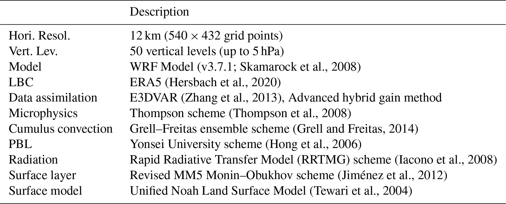
In this study, the Advanced Research WRF model (v3.7.1) is used with 12 km horizontal resolution (540 × 432 grid points) and 50 vertical levels (up to 5 hPa) for the East Asia domain shown in Fig. 1. The model settings and physics scheme are summarized in Table 1. Analysis fields are obtained every 6 h (00:00, 06:00, 12:00, and 18:00 UTC) via assimilation of conventional observations with a 6 h assimilation window, and forecast fields are integrated up to 36 h. The ERA5 reanalysis (Hersbach et al., 2020) is used as the first initial condition before the cycling and as boundary conditions every 6 h.

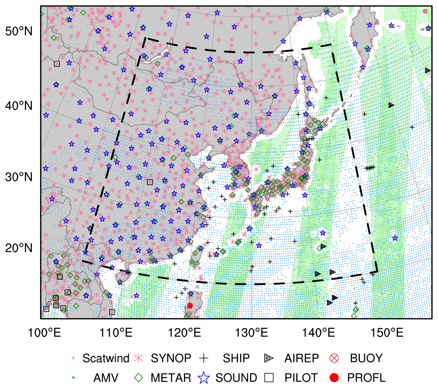
Figure 1 The East Asia Regional Reanalysis domain. The dashed black box denotes a verification area. Different types of NCEP PrepBUFR observations are available for assimilation at 00:00 UTC on 1 January 2017.

Table 1 Model configuration.

2.2 Data assimilation methods

2.2.1 E3DVAR

The E3DVAR method is one of the hybrid DA methods that use a static climatological background error covariance (BEC) and ensemble-based flow-dependent BEC, and couples the EnKF and 3DVAR (Zhang et al., 2013). E3DVAR is based on a cost function of 3DVAR. In E3DVAR, EnKF provides flow-dependent BEC as well as updates on perturbations for ensemble members. Following Zhang et al. (2013),

$$\begin{array}{}\text{(1)}& J^{\mathrm{b}}=J_{\mathrm{s}}^{\mathrm{b}}+J_{\mathrm{e}}^{\mathrm{b}}={\displaystyle \frac{\mathrm{1}}{\mathrm{2}}}\mathit{\delta }{\mathit{x}}^{\mathrm{T}}{\left[(\mathrm{1}-\mathit{\beta })\mathbf{B}+\mathit{\beta }{\mathbf{P}}^{\mathrm{f}}\circ \mathbf{C}\right]}^{-\mathrm{1}}\mathit{\delta }\mathit{x},\end{array}$$

where $J_{\mathrm{s}}^{\mathrm{b}}$ is a traditional cost function based on a static climatological BEC B and $J_{\mathrm{e}}^{\mathrm{b}}$ is an additional cost function based on ensemble-based BEC P^f. C is a correlation matrix for localization of the ensemble covariance P^f. The weighting coefficient β between static and ensemble-based BEC is set to 0.8 in this study. To account for model error for E3DVAR, a multi-physics scheme is applied to 40-member ensembles. Yang and Kim (2021a) found that E3DVAR is the most appropriate DA method among 3DVAR, EnKF, and E3DVAR methods over East Asia. More detailed information on E3DVAR implemented in this study can be found in Yang and Kim (2021a).

2.2.2 Hybrid gain data assimilation method

In the last decade, the traditional hybrid methods have been widely used for many operational centers and research institutes. Recently, Penny (2014) proposed a new class of hybrid gain methods combining desirable aspects of both variational and EnKF families of algorithms by weighting analyses from 3DVAR and LETKF for an optimal analysis in the Lorenz 40-component model. Since then, this algorithm has been implemented at ECMWF (Bonavita et al., 2015) and at a hybrid global ocean DA system in the National Centers for Environmental Prediction (NCEP) (Penny et al., 2015).

The hybrid gain algorithm can be described with the following equations:

$$\begin{array}{}\text{(2)}& {\mathit{x}}_{\mathrm{Hyb}}^{\mathrm{a}}=\mathit{\alpha }{\mathit{x}}_{\mathrm{Det}}^{\mathrm{a}}+(\mathrm{1}-\mathit{\alpha })\stackrel{\mathrm{‾}}{{\mathit{x}}^{\mathrm{a}}},\end{array}$$

where ${\mathit{x}}_{\mathrm{Hyb}}^{\mathrm{a}}$, ${\mathit{x}}_{\mathrm{Det}}^{\mathrm{a}}$, and $\stackrel{\mathrm{‾}}{{\mathit{x}}^{\mathrm{a}}}$ denote the hybrid analysis, deterministic analysis, and the ensemble mean analysis from the ensemble-based assimilation method, and α is a tunable parameter (Penny, 2014; Houtekamer and Zhang, 2016).

The hybrid gain method is different from traditional hybrid methods, in that a hybrid gain approach linearly combines analysis fields from EnKF and variational DA methods to produce a hybrid gain analysis rather than linearly combining respective BECs (Penny, 2014). Basically, the hybrid gain method is used to hybridize two different Kalman gain matrices of ensemble-based (Eq. 4) and variational DA systems (Eq. 5) as in Eq. (3):

$$\begin{array}{}\text{(3)}& \widehat{\mathbf{K}}={\mathit{\beta }}_{\mathrm{1}}{\mathbf{K}}^{\mathrm{f}}+{\mathit{\beta }}_{\mathrm{2}}{\mathbf{K}}^{\mathrm{B}}+{\mathit{\beta }}_{\mathrm{3}}{\mathbf{K}}^{\mathrm{B}}{\mathbf{HK}}^{\mathrm{f}},\end{array}$$

where

$$\begin{array}{}\text{(4)}& {\displaystyle }{\mathbf{K}}^{\mathrm{f}}={\mathbf{P}}^{\mathrm{f}}{\mathbf{H}}^{\mathrm{T}}({\mathbf{HP}}^{\mathrm{f}}{\mathbf{H}}^{\mathrm{T}}+\mathbf{R}{)}^{-\mathrm{1}},\text{(5)}& {\displaystyle }{\mathbf{K}}^{\mathrm{B}}={\mathbf{BH}}^{\mathrm{T}}({\mathbf{HBH}}^{\mathrm{T}}+\mathbf{R}{)}^{-\mathrm{1}}.\end{array}$$

H is an observation operator mapping the model state vector to observation space and R is the observation error covariance matrix. The matrices P^f and B indicate the ensemble-based and the static climatological BEC, respectively. By choosing the specific coefficients (β₁=1, β₂=α, ${\mathit{\beta }}_{\mathrm{3}}=-\mathit{\alpha }$), it can be written as in Eq. (6) and it can give an algebraically equivalent result with Eq. (2) (Penny, 2014):

$$\begin{array}{}\text{(6)}& \widehat{\mathbf{K}}={\mathbf{K}}^{\mathrm{f}}+\mathit{\alpha }{\mathbf{K}}^{\mathrm{B}}(\mathbf{I}-{\mathbf{HK}}^{\mathrm{f}}).\end{array}$$

One of the advantages of the hybrid gain algorithm with respect to its development is that preexisting operational systems can be used without significant modification for a hybrid analysis (Penny, 2014) and independent parallel development of respective methods is allowed (Houtekamer and Zhang, 2016). Furthermore, the hybrid gain approach can be considered a practical and straightforward method in the foreseeable future to combine advantageous features of both ensemble- and variational-based DA algorithms (Houtekamer and Zhang, 2016). More detailed information on this algorithm can be found in Penny (2014).

2.2.3 Advanced hybrid gain data assimilation method

In this study, based on the hybrid gain approach, an advanced hybrid gain DA method (AdvHG) is newly proposed as follows:

$$\begin{array}{}\text{(7)}& X_{\mathrm{AdvHG}}^{\mathrm{a}}=\mathit{\alpha }{X}_{\mathrm{ERA}\mathrm{5}}^{f\left(\mathrm{6}\mathrm{h}\right)}+(\mathrm{1}-\mathit{\alpha }){\stackrel{\mathrm{‾}}{X}}_{\mathrm{E}\mathrm{3}\mathrm{DVAR}}^{\mathrm{a}},\end{array}$$

where $X_{\mathrm{ERA}\mathrm{5}}^{f\left(\mathrm{6}\mathrm{h}\right)}$ denotes the 6 h forecast of ERA5 reanalysis based on the WRF model and ${\stackrel{\mathrm{‾}}{X}}_{\mathrm{E}\mathrm{3}\mathrm{DVAR}}^{\mathrm{a}}$denotes the analysis of E3DVAR (Fig. 2). In Eq. (7), α is a tunable parameter and is assigned to be 0.5 in this study. This advanced hybrid gain approach is different from the hybrid gain approach in that (1) E3DVAR analysis is used instead of EnKF, (2) 6 h forecast of ERA5 is used instead of deterministic analysis from the variational DA method, and (3) the preexisting and state-of-the-art reanalysis data (i.e., ERA5) are simply used instead of producing deterministic analysis by assimilation. The reasons for these different approaches proposed in this study are as follows:

1. E3DVAR is used instead of EnKF because Yang and Kim (2021a) confirmed that E3DVAR outperforms EnKF for winter and summer seasons over East Asia.

2. Instead of deterministic analysis, the 6 h forecast of ERA5 based on the WRF model is used to make the hybrid analysis more balanced and consistent with the WRF model, because ERA5 reanalysis fields are based on its own modeling system with coarser resolution, which is different from that used in this study.

3. European Centre for Medium-Range Weather Forecasts (ECMWF) reanalysis (ERA5) is used instead of producing our own analysis fields from a variational DA method. This is a very efficient approach because of the cost savings as well as the use of the high-quality latest reanalysis from ECMWF assimilating all currently available observations with the state-of-the-art and advanced technology.

Therefore, the approach proposed in this study is called “advanced hybrid gain method” (denoted as “AdvHG”).

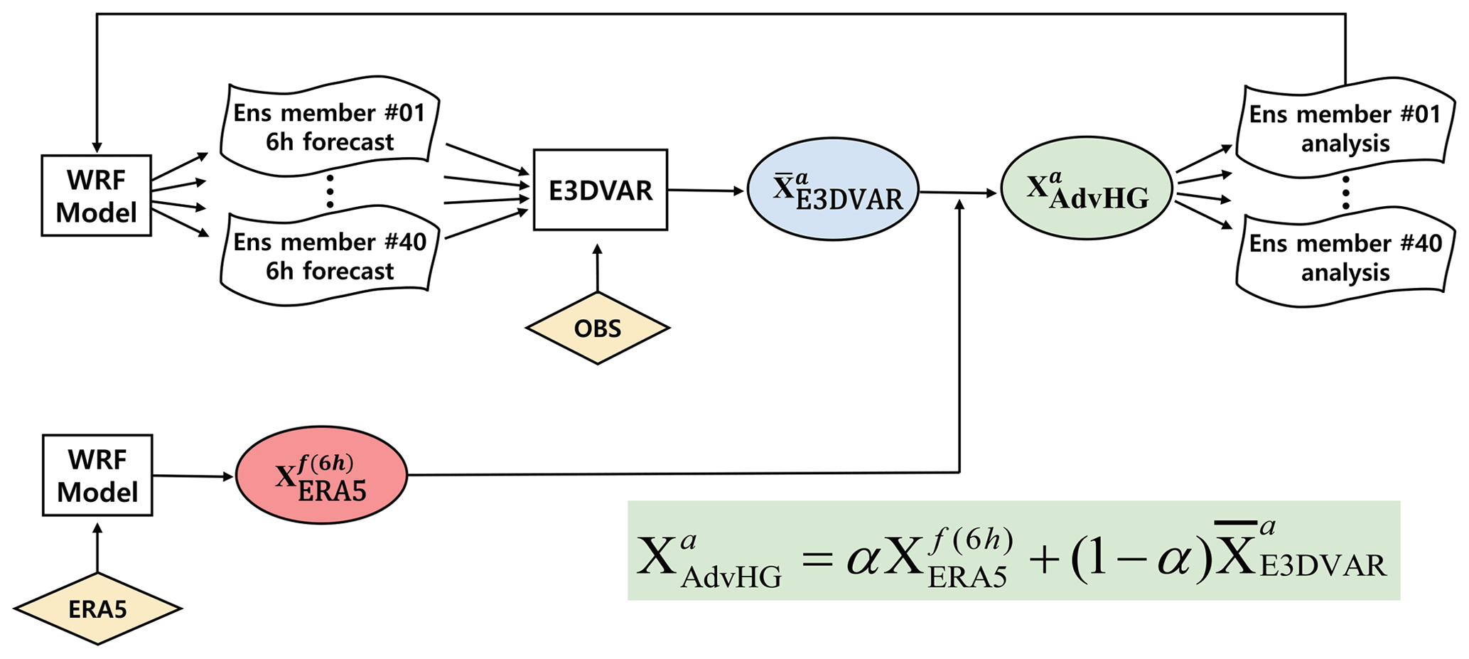
Figure 2 Schematic diagram of the advanced hybrid gain data assimilation method in the East Asia Regional Reanalysis system.

2.3 Observations

The NCEP PrepBUFR (Prepared or QC'd data in BUFR (Binary Universal Form for the Representation of meteorological data) format) conventional observations (global upper-air and surface weather observations, NCEP/NWS/NOAA/U.S.DOC, 2008) are used every 6 h (00:00, 06:00, 12:00, and 18:00 UTC) for an assimilation by E3DVAR and AdvHG methods (Fig. 1). The PrepBUFR is the output of the final process for preparing the observations to be assimilated in the different NCEP analyses. For observations, rudimentary multi-platform quality control (QC) and more complex platform-specific QCs were conducted (e.g., surface pressure, rawinsonde heights and temperature, wind profiler, aircraft wind and temperature) in NCEP (Keyser, 2013). Furthermore, if the innovations (i.e., observation minus background) of some observations are greater than 5 times the observational error, then that observation is rejected during the assimilation procedure in this study.

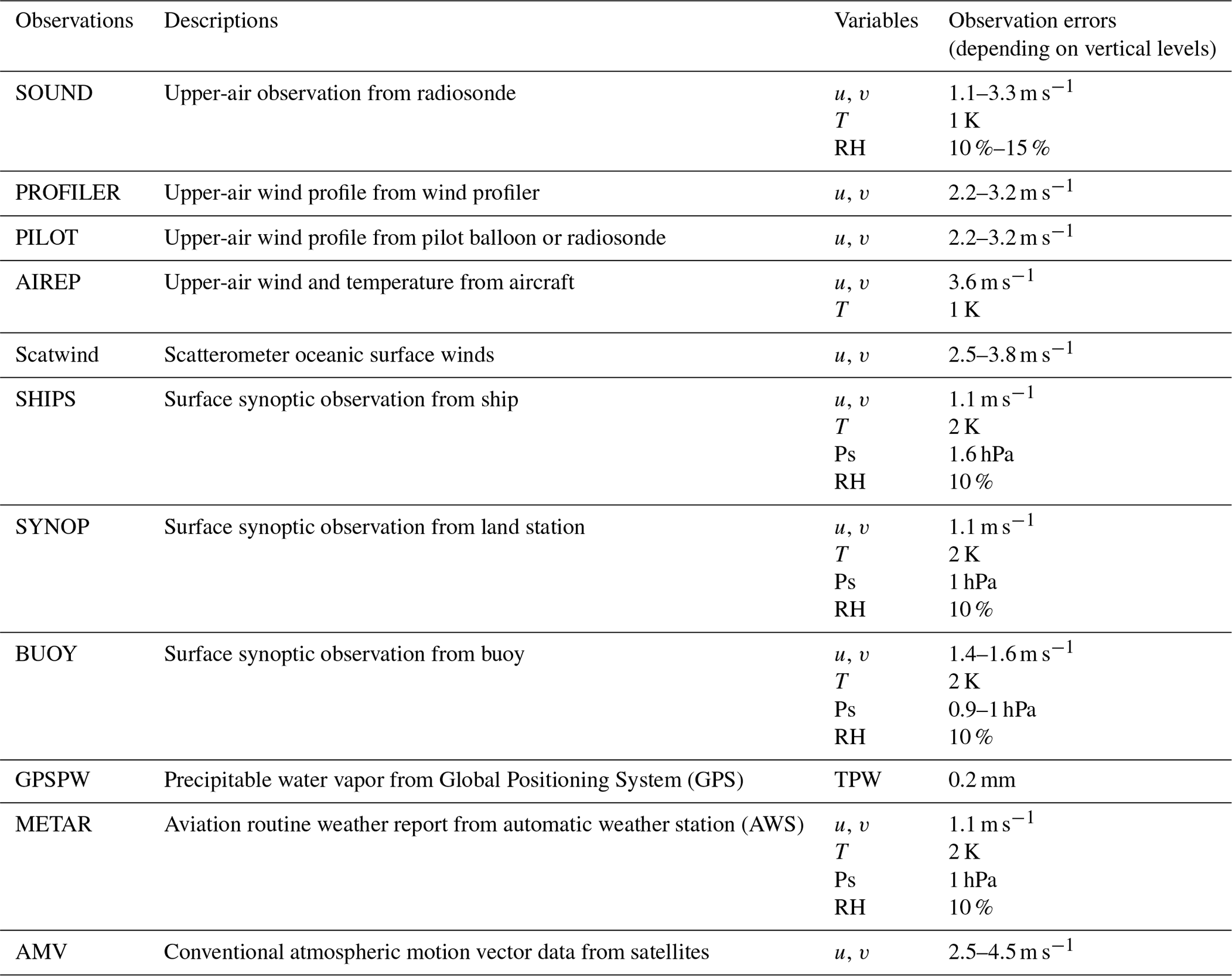
The assimilated observations are as follows: the surface observations (SYNOP, METAR, Ship, and Buoy), radiosonde observation (SOUND), upper-wind report (PILOT), wind profiler, aircraft, atmospheric motion vector (AMV) wind from satellites, scatterometer oceanic surface winds (Scatwind), and precipitable water vapor from the Global Positioning System (GPSPW). The observation errors depending on each observation platform, variable, and vertical levels are assigned based on the default observation error statistics provided in the WRFDA system (Table 2). All observations are spatially thinned by 20 km except for AMV thinned by 200 km, as done by Warrick (2015), Cotton et al. (2016), and Shin et al. (2016).

Table 2 Summary of observations used in this study. The default observation error statistics provided in the WRFDA system are used for assimilation in this study. The variables u, v, T, RH, Ps, and TPW denote zonal wind, meridional wind, temperature, relative humidity, surface pressure, and total precipitable water, respectively.

To evaluate 6 h accumulated precipitation simulated by E3DVAR, AdvHG, ERA-I, and ERA5 over East Asia, global surface weather observations (NCEP PrepBUFR, NCEP/NWS/NOAA/U.S.DOC, 2008) are used every 6 h (00:00, 06:00, 12:00, and 18:00 UTC). For an evaluation of the monthly precipitation fields, the World Monthly Surface Station Climatology (NCDC/NESDIS/NOAA/U.S.DOC et al., 1981) over 4700 different stations (2600 in more recent years) is used.

2.4 Global reanalysis datasets

To compare EARR generated with other reanalysis datasets, ERA5 (Hersbach et al., 2020) and ERA-I (Dee et al., 2011) reanalyses are chosen. The horizontal resolutions of ERA-I and ERA5 are approximately 79 (TL255) and 31 km (TL639), respectively. Because ERA5 is based on the operational system in 2016, improvements in model physics, numerics, data assimilation, and additional observations over the last decade are the advantages of ERA5 (Hersbach et al., 2018).

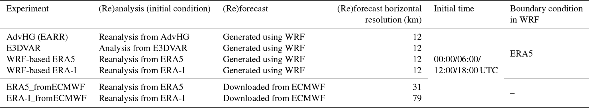
In this study, (re)forecast as well as reanalysis fields need to be verified. Regarding reanalysis and (re)forecast fields of ECMWF, reanalysis fields (i.e., ERA5 and ERA-I) downloaded from ECMWF are evaluated (Figs. 3 and 6). Two different (re)forecast fields (e.g., ERA5_fromECMWF, WRF-based ERA5) are used in this study. WRF-based ERA5 and ERA-I are forecast fields based on the WRF model with 12 km horizontal resolution where ERA5 and ERA-I are used as initial conditions. By contrast, ERA5_fromECMWF and ERA-I_fromECMWF are reforecast fields based on the ECMWF model not the WRF model, and thus the reforecast fields of ERA5 and ERA-I are provided and downloaded from ECMWF. These reforecast fields are only used for evaluation of precipitation (Figs. 8 and 9). The (re)analysis and (re)forecast fields and corresponding experiments are explained in Table 3.

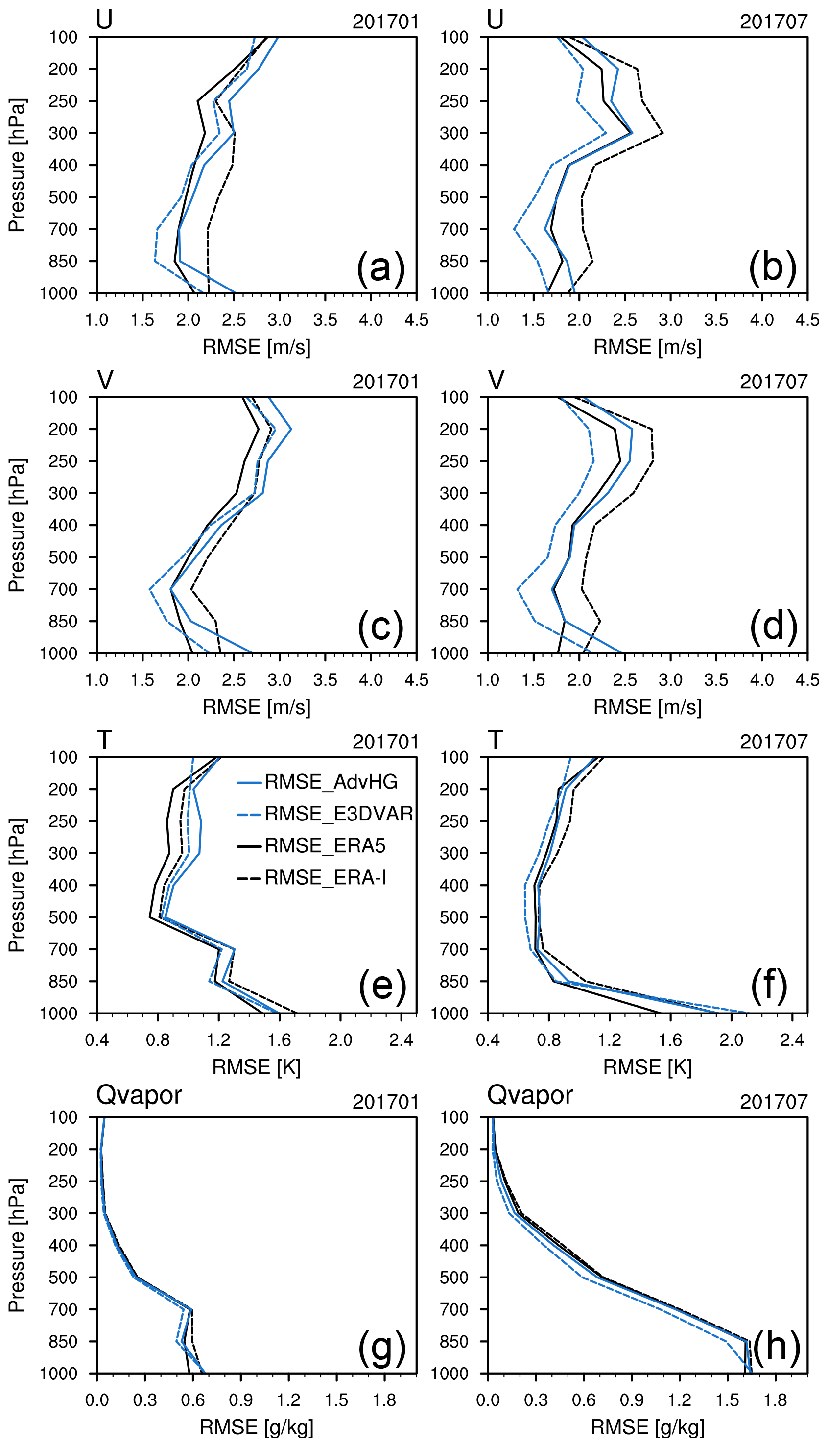
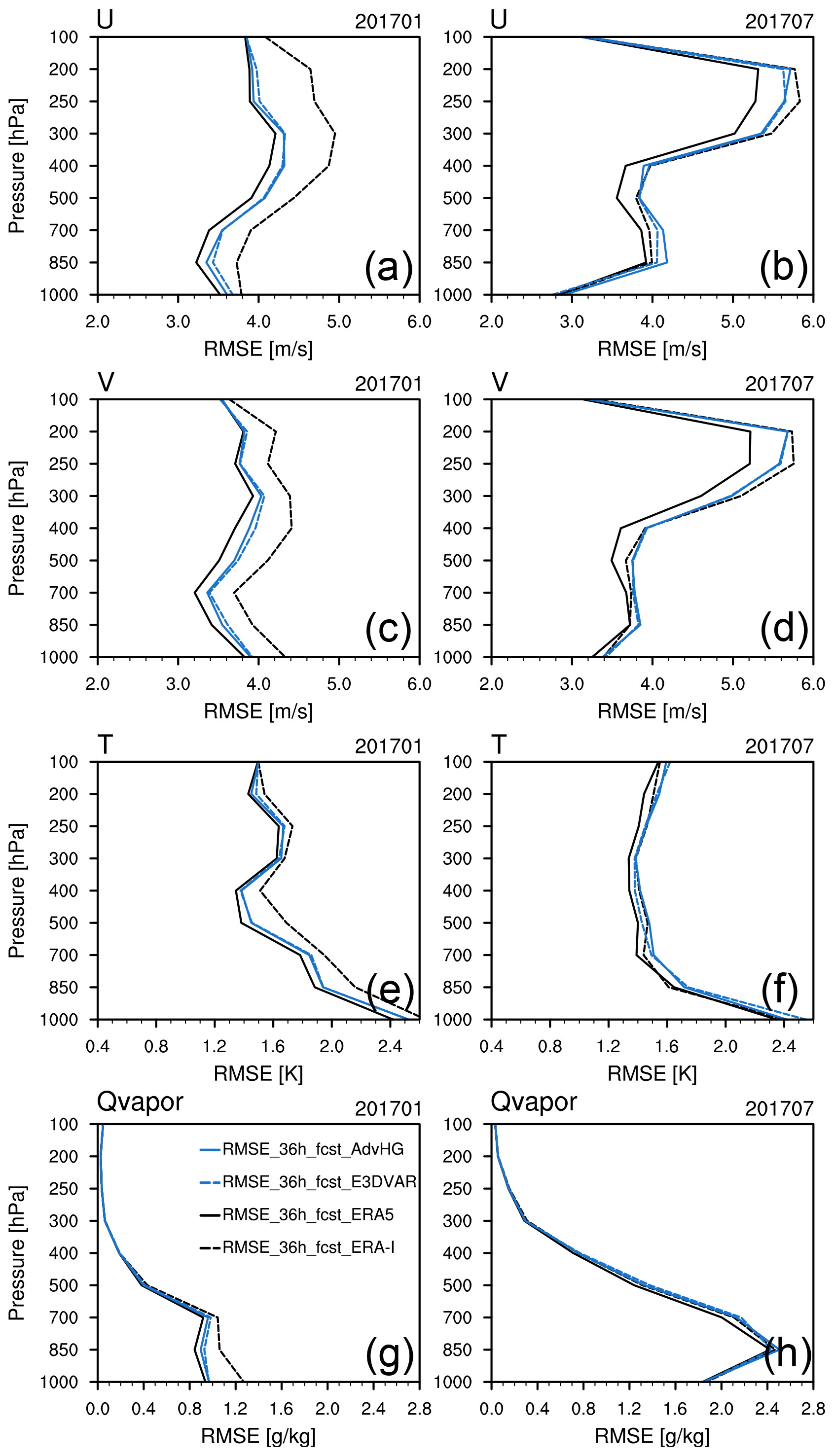
Figure 3 RMSEs in analysis of (a, b) zonal wind, (c, d) meridional wind, (e, f) temperature, and (g, h) Qvapor (water vapor mixing ratio) from ERA-I (dashed black line), ERA5 (solid black line), E3DVAR (dashed blue line), and AdvHG (solid blue line) depending on pressure levels for (a, c, e, g) January and (b, d, f, h) July 2017.

Table 3 (Re)analyses and (re)forecasts with corresponding experiments used in this study.

3 Evaluation method

3.1 Equitable threat score and frequency bias index

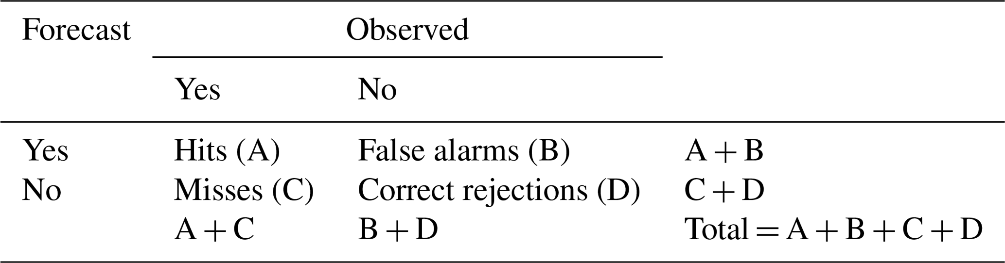
Based on the contingency table (Table 4), ETS is defined as

$$\begin{array}{}\text{(8)}& \mathrm{ETS}={\displaystyle \frac{\mathrm{A}-{\mathrm{A}}_{\mathrm{r}}}{\mathrm{A}+\mathrm{B}+\mathrm{C}-{\mathrm{A}}_{\mathrm{r}}}},\text{where}{\mathrm{A}}_{\mathrm{r}}={\displaystyle \frac{(\mathrm{A}+\mathrm{B})(\mathrm{A}+\mathrm{C})}{\mathrm{A}+\mathrm{B}+\mathrm{C}+\mathrm{D}}}.\end{array}$$

The ETS range is from $-\mathrm{1}/\mathrm{3}$ to 1 and the value 1 for ETS is a perfect score. ETS is a more balanced score than probability of detection (POD) and false alarm ratio (FAR) because it is sensitive to both false alarms and misses (Wilson, 2017).

FBI is defined as

$$\begin{array}{}\text{(9)}& \mathrm{FBI}=\mathrm{Bias}={\displaystyle \frac{\mathrm{A}+\mathrm{B}}{\mathrm{A}+\mathrm{C}}}.\end{array}$$

The FBI indicates whether the model tends to over-forecast (too frequently, FBI >1) or under-forecast (not frequent enough, FBI <1) events with respect to frequency of occurrence.

Table 4 The 2×2 contingency table for dichotomous (yes–no) events.

3.2 Probability of detection and false alarm ratio

Based on the contingency table (Table 4), POD is defined as

$$\begin{array}{}\text{(10)}& \mathrm{POD}={\displaystyle \frac{\mathrm{A}}{\mathrm{A}+\mathrm{C}}}={\displaystyle \frac{\mathrm{Hits}}{\mathrm{Hits}+\mathrm{Misses}}}.\end{array}$$

The POD range is from 0 to 1. POD is required to be used with FAR because POD can be artificially improved by systematically over-forecasting the events (Wilson, 2017).

FAR is defined as

$$\begin{array}{}\text{(11)}& \mathrm{FAR}={\displaystyle \frac{\mathrm{B}}{\mathrm{A}+\mathrm{B}}}={\displaystyle \frac{\text{False alarms}}{\mathrm{Hits}+\text{False alarms}}}.\end{array}$$

The range of FAR is from 0 to 1 and its lower score implies a higher accuracy.

3.3 Brier skill score

Verification of the performance of high-resolution forecast with the traditional verification metrics (e.g., ETS, FBI) can be misleading due to a double penalty, particularly for highly variable fields (e.g., precipitation). Therefore, as one of the spatial verification approaches that do not require forecast to match point observation spatially, the neighborhood (fuzzy) verification method, which assumes that a slightly displaced forecast can be acceptable and a local neighborhood can define the degree of allowable displacement (Ebert, 2008; Kim et al., 2015; On et al., 2018), is used in this section. According to Ebert (2008), depending on the matching strategy, neighborhood verifications can be categorized into two frameworks: “single observation–neighborhood forecast (SO-NF)” where neighborhood forecasts surrounding observations are considered, and “neighborhood observation–neighborhood forecast (NO-NF)” strategies where not only neighborhood forecasts but also neighborhood observations surrounding observations are considered. Due to the absence of high-resolution gridded precipitation observation data in East Asia, various verification scores widely used as an NO-NF strategy are not available in this study. Thus, in this section, the Brier skill score (BSS), as one of the SO-NF strategies, is introduced.

The Brier score (BS) is similar to the mean squared error (MSE) and is defined as (Wilks, 2006)

$$\begin{array}{}\text{(12)}& \mathrm{BS}={\displaystyle \frac{\mathrm{1}}{N}}\sum _{i=\mathrm{1}}^N(p_i-o_i{)}^{\mathrm{2}},\end{array}$$

where p_i denotes the probability forecast, o_i denotes the binary observation which is either 0 or 1, and N is the total number of observations during the given period. Generally, the BSS (or BS) is used to verify ensemble forecasts which are able to calculate probabilistic forecasts (Kay et al., 2013; Kim and Kim, 2017). However, the BSS can also be used for deterministic forecasts using a pragmatic post-processing procedure (Theis et al., 2005; Mittermaier, 2014), which derives probabilistic forecasts from deterministic forecasts at every model grid point by considering neighborhood forecast as pseudo ensemble:

$$\begin{array}{}\text{(13)}& \mathrm{BSS}=\mathrm{1}-{\displaystyle \frac{\mathrm{BS}}{{\mathrm{BS}}_{\mathrm{ref}}}},\end{array}$$

where BS_ref is the BS of reference. The BSS is the skill score with respect to the BS as in Eq. (13). For reference, a climatology or other forecast can be used. In this study, the WRF-based ERA-I is considered as a reference.

3.4 Pattern correlation coefficient

The pattern correlation coefficient (PCC) is defined as Eq. (14) (Shiferaw et al., 2018; Yoo and Cho, 2018; Park and Kim, 2020),

$$\begin{array}{}\text{(14)}& \mathrm{PCC}={\displaystyle \frac{\sum _{i=\mathrm{1}}^N(x_i-\stackrel{\mathrm{‾}}{x})(o_i-\stackrel{\mathrm{‾}}{o})}{{\left[\sum _{i=\mathrm{1}}^N(x_i-\stackrel{\mathrm{‾}}{x}{)}^{\mathrm{2}}\sum _{i=\mathrm{1}}^N(o_i-\stackrel{\mathrm{‾}}{o}{)}^{\mathrm{2}}\right]}^{\mathrm{1}/\mathrm{2}}}},\end{array}$$

where x_i and o_i are (re)forecast and observed precipitation at ith observation location and the over-bar indicates the averaged variables over N observed stations in the verification area.

4 Results

4.1 Evaluation of wind, temperature, and humidity variables

4.1.1 RMSE for January and July 2017

The analysis and forecast RMSEs of E3DVAR, AdvHG, the WRF-based ERA-I, and WRF-based ERA5 are calculated for zonal wind, meridional wind, temperature, and Qvapor (water vapor mixing ratio in WRF) variables against sonde observations at 00:00 and 12:00 UTC in verification domain (dashed box in Fig. 1) for January and July 2017 and averaged over each month (Figs. 3, 4, and 5).

For the analysis RMSE (Fig. 3), E3DVAR is smaller than AdvHG for all pressure levels and variables, except for temperature in July at 1000 hPa and Qvapor in January and July at 1000 hPa. In general, the analysis RMSE of AdvHG for all variables is comparable to or greater than that of ERA5. The analysis RMSE of ERA5 is smaller than that of ERA-I for all levels and variables; in particular, the analysis RMSE difference between ERA5 and ERA-I is distinctive for wind.

Regarding wind variables of analysis (Fig. 3a, b, c, and d), E3DVAR is the most closely fitted to observations except for the wind in the upper troposphere in January, followed by ERA5, AdvHG, and ERA-I. For the temperature RMSE (Fig. 3e and f), E3DVAR is smaller than AdvHG. For Qvapor, RMSE in July is much larger than that in January due to a monsoonal flow carrying moist air to East Asia. In general, the Qvapor RMSE of E3DVAR is the smallest, followed by ERA5, AdvHG, and ERA-I. Therefore, for all variables, E3DVAR analysis fields are generally the most closely fitted to observations. Since the analysis RMSE implies how much the analysis fields are fitted to observations rather than the accuracy of analysis itself, not only the analysis RMSE but also the forecast RMSE should be considered.

For 24 h forecast fields in January (Fig. 4a, c, e, and g), overall, the RMSEs of AdvHG and E3DVAR are greater than those of ERA5 and smaller than those of ERA-I, and the AdvHG RMSE is smaller than the E3DVAR RMSE for all levels and variables. Meanwhile, for July (Fig. 4b, d, f, and h), AdvHG and E3DVAR show comparable RMSE to ERA-I.

Figure 4 The same RMSEs as in Fig. 3, except for 24 h forecast.

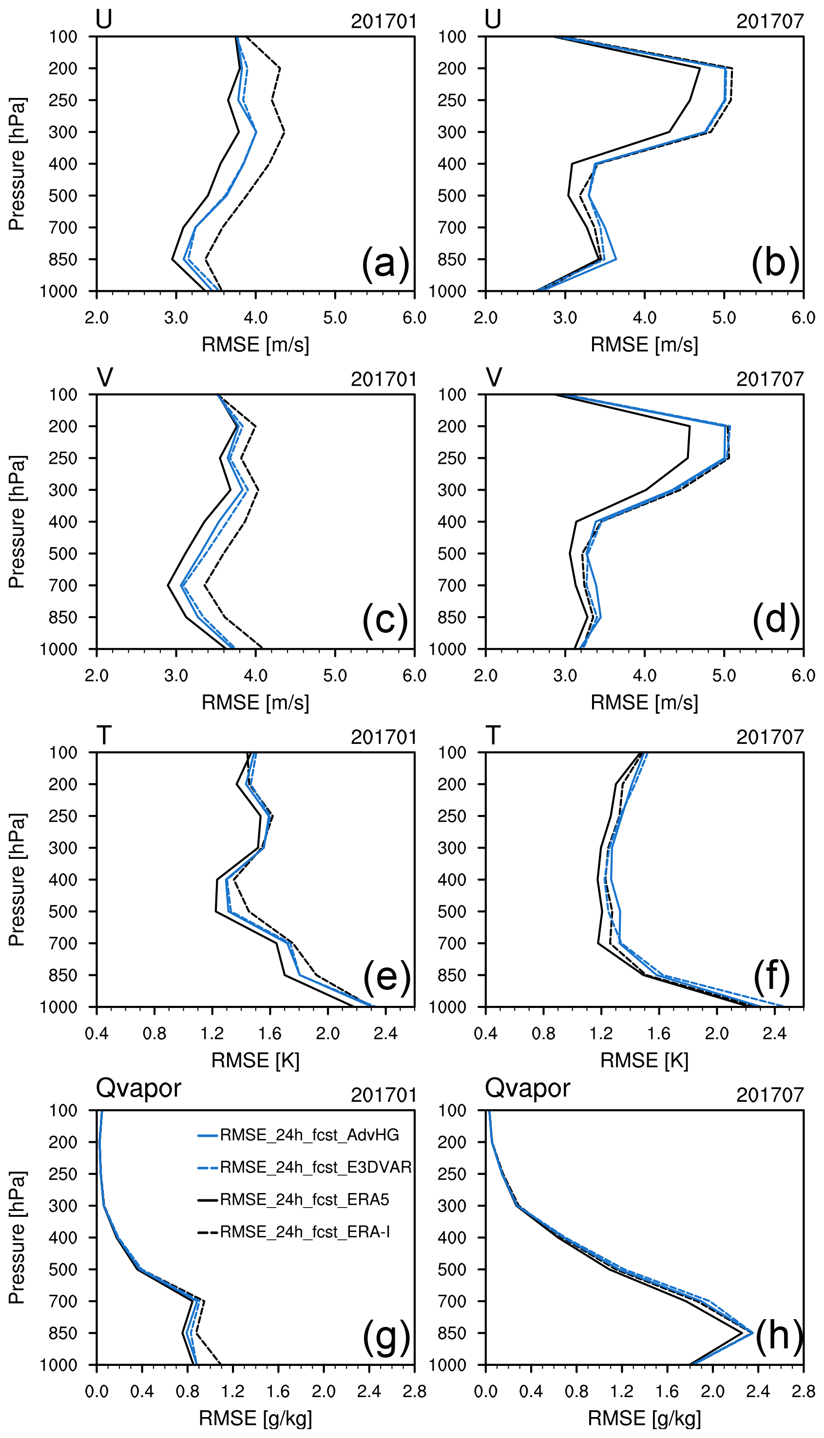
Furthermore, the general features of the 36 h forecast RMSE (Fig. 5) are similar to the 24 h forecast RMSE (Fig. 4). However, particularly in January, the 36 h forecast RMSE differences between ERA5 and ERA-I are more distinctive than those of the 24 h forecast. In January, the vertically averaged 36 h forecast RMSE differences of ERA5 and ERA-I are 0.52 m s⁻¹ for wind, 0.16 K for temperature, and 0.08 g kg⁻¹ for Qvapor, whereas those of the 24 h forecast are 0.4 m s⁻¹ for wind, 0.11 K for temperature, and 0.06 g kg⁻¹ for Qvapor. In addition, the 36 h forecast RMSE differences between ERA5 and AdvHG for January are on average 0.1 m s⁻¹ for wind, 0.05 K for temperature, and 0.02 g kg⁻¹ for Qvapor, which are even smaller compared to those of the 24 h forecast, implying that AdvHG is much more accurate than ERA-I for January 2017. For July, the 36 h forecast RMSE of ERA5 is the smallest and the RMSEs of AdvHG and E3DVAR are similar to those of ERA-I.

Figure 5 The same RMSEs as in Fig. 3, except for 36 h forecast.

4.1.2 RMSE and spread for the period 2010–2019

In this section, the EARR produced in this study is verified for a longer period with WRF-based ERA5. The RMSE and spread of reanalyses and reforecasts based on the AdvHG method are calculated and averaged over the period 2010–2019. The reanalyses and (re)forecast fields are evaluated by calculating RMSE valid at 00:00 and 12:00 UTC and spread at 00:00, 06:00, 12:00, and 18:00 UTC.

The averaged RMSEs of reanalysis for ERA5 and EARR (denoted as AdvHG in Fig. 6) and spread of analysis and 6 h forecast fields of EARR (AdvHG) are shown in Fig. 6. With respect to spread, the ensemble spreads of analysis fields are smaller than those of 6 h forecast fields, on average, by 0.15 m s⁻¹ for wind, 0.04 K for temperature, and 0.02 g kg⁻¹ for Qvapor, which is the well-known characteristic of ensemble-based DA methods. Specifically, the wind spread (Fig. 6a and b) is similar to or greater than the wind RMSE except for the upper troposphere above 200 hPa, implying the ensemble spread for wind is well represented below 200 hPa. On the contrary, the ensembles for temperature and Qvapor (Fig. 6c and d) are underdispersive compared to their RMSEs.

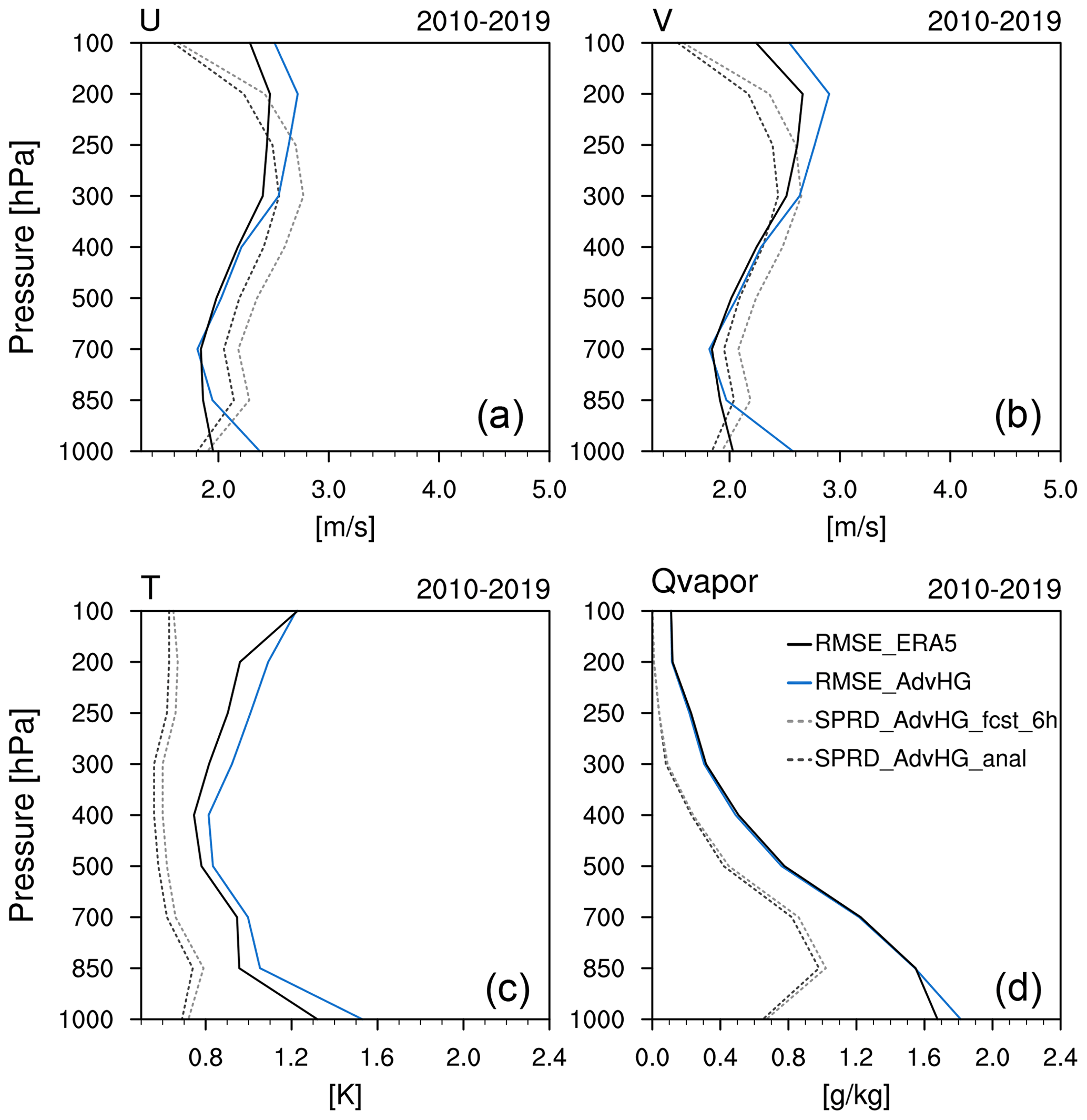
Figure 6 RMSEs of analysis of (a) zonal wind, (b) meridional wind, (c) temperature, and (d) Qvapor (water vapor mixing ratio) from ERA5 (solid black line) and AdvHG (solid blue line) and spreads of analysis (dashed black line) and 6 h forecast (dashed gray line) of AdvHG depending on pressure levels averaged over the 10-year period 2010–2019.

Regarding the reanalysis RMSE, overall AdvHG RMSE is greater than ERA5 RMSE for all variables (Fig. 6). The vertically averaged RMSEs of AdvHG are greater by 0.16 m s⁻¹ for wind, 0.09 K for temperature, and 0.01 g kg⁻¹ for Qvapor than those of ERA5. Nonetheless, the wind RMSEs of AdvHG are similar to those of ERA5 for the middle of the troposphere (400–850 hPa), and the Qvapor RMSEs of AdvHG are similar to those of ERA5 except for 1000 hPa.

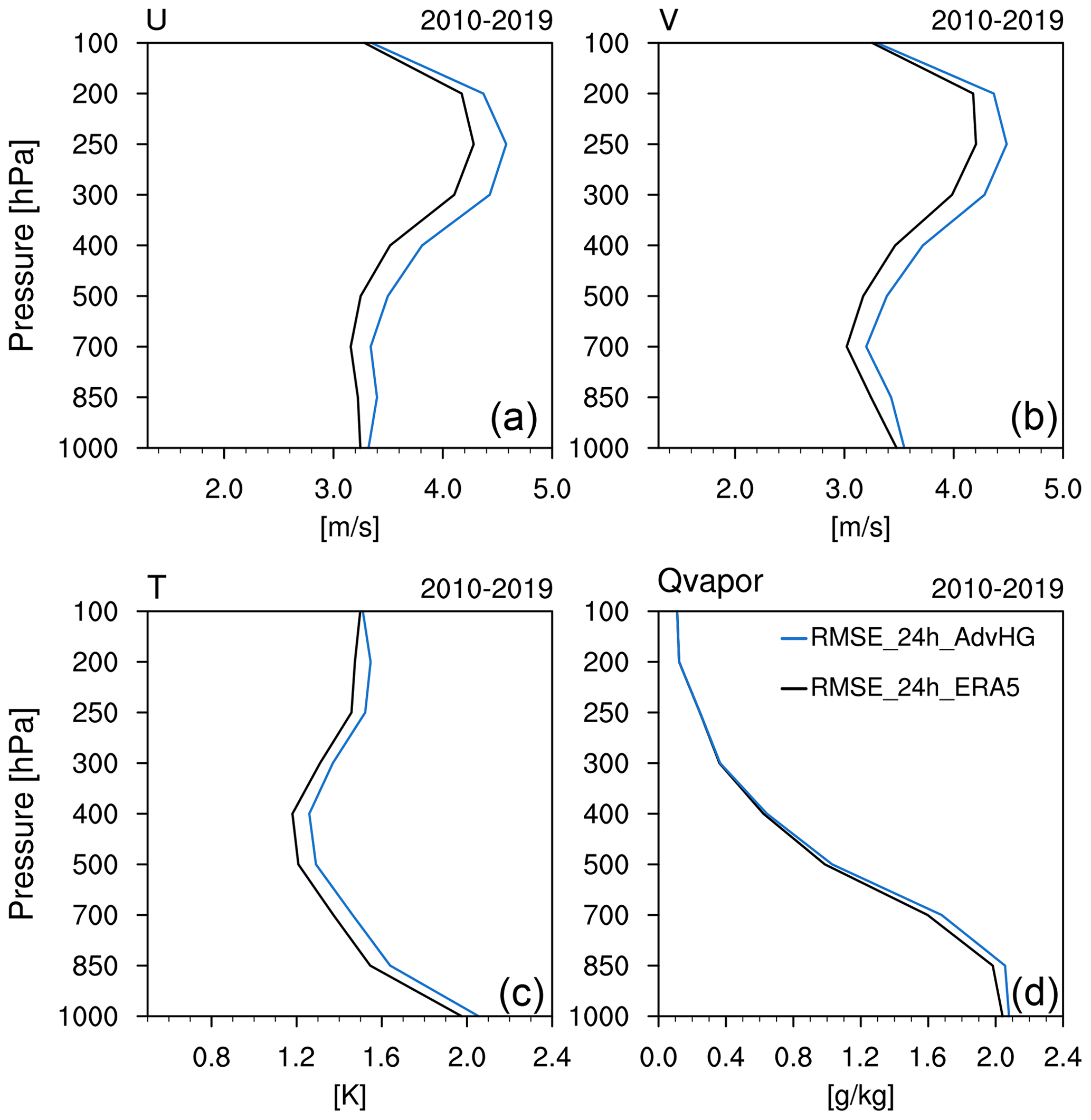
In addition, regarding the 24 h forecast RMSE, AdvHG shows a larger RMSE than ERA5 for all variables (Fig. 7). The vertically averaged RMSE differences of wind, temperature, and Qvapor variables between AdvHG and ERA5 are approximately 0.2 m s⁻¹, 0.07 K, and 0.03 g kg⁻¹, respectively. These differences are smaller, compared to the 24 h forecast RMSE difference between ERA-I and ERA5 shown in Fig. 4 (i.e., wind, temperature, and Qvapor RMSE difference: 0.4 m s⁻¹, 0.11 K, and 0.06 g kg⁻¹ for January 2017, 0.25 m s⁻¹, 0.05 K, and 0.04 g kg⁻¹ for July 2017).

Figure 7 The same RMSEs as in Fig. 6, except for RMSEs of 24 h forecast.

4.2 Evaluation of precipitation for January and July in 2017

4.2.1 Evaluation metrics

Equitable threat score and frequency bias index

In​​​​​​​ this section, for the point-based equitable threat score (ETS) and frequency bias index (FBI) based on Table 4, the 6 h accumulated precipitation fields based on the 6 h forecast of E3DVAR, AdvHG, WRF-based ERA-I, WRF-based ERA5, ERA-I_fromECMWF, and ERA5_fromECMWF are evaluated every 6 h (00:00, 06:00, 12:00, and 18:00 UTC) for January and July 2017 (Fig. 8). Here, all the WRF-based precipitation fields are based on 12 km horizontal resolution, and ERA-I_fromECMWF and ERA5_fromECMWF have 79 and 31 km horizontal resolutions, respectively. Generally, ETS decreases as a threshold increases for both months (Fig. 8a and c). For January 2017 (Fig. 8a), AdvHG ETS is the greatest among others. Compared to precipitation reforecasts from ECMWF (i.e., ERA-I_fromECMWF, ERA5_fromECMWF), AdvHG shows the higher ETS, indicating that AdvHG is able to simulate more accurate precipitation fields than ERA-I and ERA5 from ECMWF in January 2017. Surprisingly, ETS of ERA5_fromECMWF for January 2017 is the lowest among all the results and is even lower than that of ERA-I_fromECMWF.

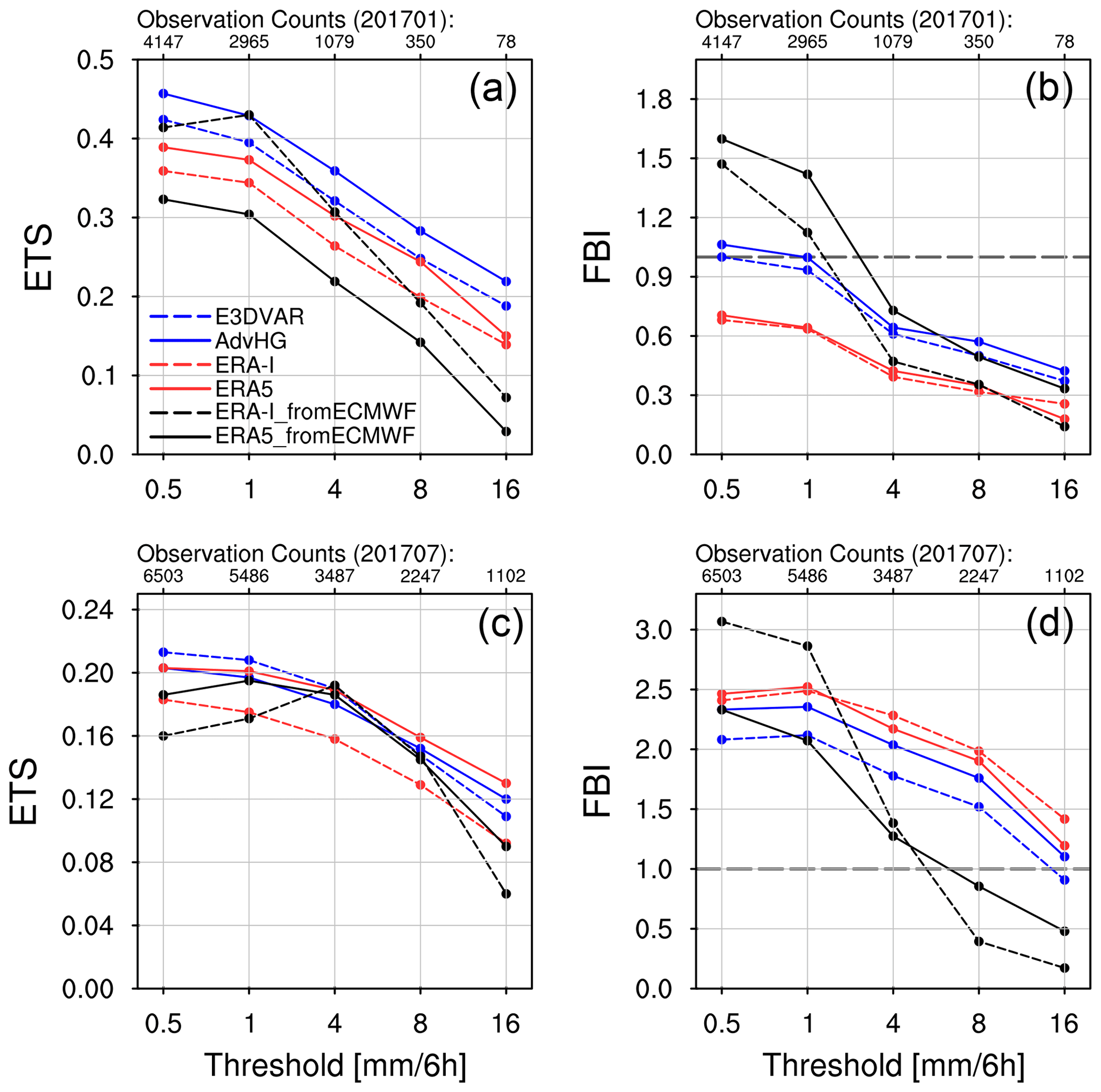
Figure 8 (a, c) ETS and (b, d) FBI for (a, b) January and (c, d) July 2017 depending on thresholds 0.5, 1, 4, 8, and 16 mm per 6 h.

Since the precipitation reforecasts from ECMWF have not only coarser resolutions but also a different forecast model (i.e., the forecasting system of ECMWF), the precipitation forecasts of ERA5 and ERA-I are additionally produced by using the same forecast model with the same resolution as AdvHG and E3DVAR in this study, as explained in Sect. 2.4. For January 2017 (Fig. 8a), ETS of ERA5 (i.e., WRF-based ERA5) is higher than that of ERA5_fromECMWF for all thresholds, whereas ETS of ERA-I (i.e., WRF-based ERA-I) is lower than that of ERA-I_fromECMWF except for high thresholds (8 and 16 mm per 6 h). The ERA5 ETS is greater than the ERA-I ETS, but is smaller than the AdvHG ETS. The AdvHG shows the greatest ETS among others with the same resolution and forecast model, and E3DVAR, ERA5, and ERA-I follow.

Regarding FBI in winter (Fig. 8b), for 4, 8, and 16 mm per 6 h thresholds, all the results show that FBI is smaller than 1, implying an underestimation of the frequency of precipitation for high-threshold events. In general, AdvHG shows the FBI closest to 1 among all the results, which is consistent with the greatest ETS of AdvHG. The E3DVAR FBI is similar to the AdvHG FBI, and ERA5 and ERA-I FBIs are similar to each other.

Overall, the ETS values for January, whose maximum is around 0.4 (Fig. 8a), are much greater than those for July 2017, whose maximum is around 0.2 (Fig. 8c), implying that the precipitation forecast in summer is more difficult than that in winter. The ETS difference between the results in July is smaller than that in January. Particularly, for the thresholds 4 and 8 mm per 6 h, the ETSs in July are similar to each other (Fig. 8c). Except for those two thresholds, the ETS of ERA-I_fromECMWF is the smallest. At the threshold of 16 mm per 6 h, ERA5 ETS is the highest, followed by AdvHG, E3DVAR, ERA-I, ERA5_fromECMWF, and ERA-I_fromECMWF. At the threshold of 0.5 and 1 mm per 6 h, the E3DVAR ETS is the greatest, followed by ERA5, AdvHG, ERA5_fromECMWF, ERA-I, and ERA-I_fromECMWF.

With respect to FBI in July 2017, the WRF-based results yield FBIs greater than 1, whereas reforecast from ECMWF yields FBIs greater than 1 for 0.5, 1, and 4 mm per 6 h thresholds and smaller than 1 for higher thresholds (8 and 16 mm per 6 h) (Fig. 8d). For July 2017, in general, ERA5_fromECMWF FBI is the closest to 1, followed by E3DVAR, AdvHG, ERA5, ERA-I, and ERA-I_fromECMWF FBI.

Probability of detection and false alarm ratio

The probability of detection (POD or hit rate) and false alarm ratio (FAR) are calculated for precipitation simulated from E3DVAR, AdvHG, WRF-based ERA-I, WRF-based ERA5, ERA-I_fromECMWF, and ERA5_fromECMWF for January and July 2017 (Fig. 9). For January 2017, AdvHG POD is the greatest among the WRF-based results, followed by E3DVAR, ERA5, and ERA-I (Fig. 9a). In addition to the lowest ETS of ERA5_fromECMWF for January 2017 as discussed in the Sect. “Equitable threat score and frequency bias index”, the FAR of ERA5_fromECMWF is extremely high with a low POD in winter. Therefore, especially for January 2017, the precipitation fields simulated from EARR (AdvHG) over East Asia are much more accurate than those from ERA5_fromECMWF.

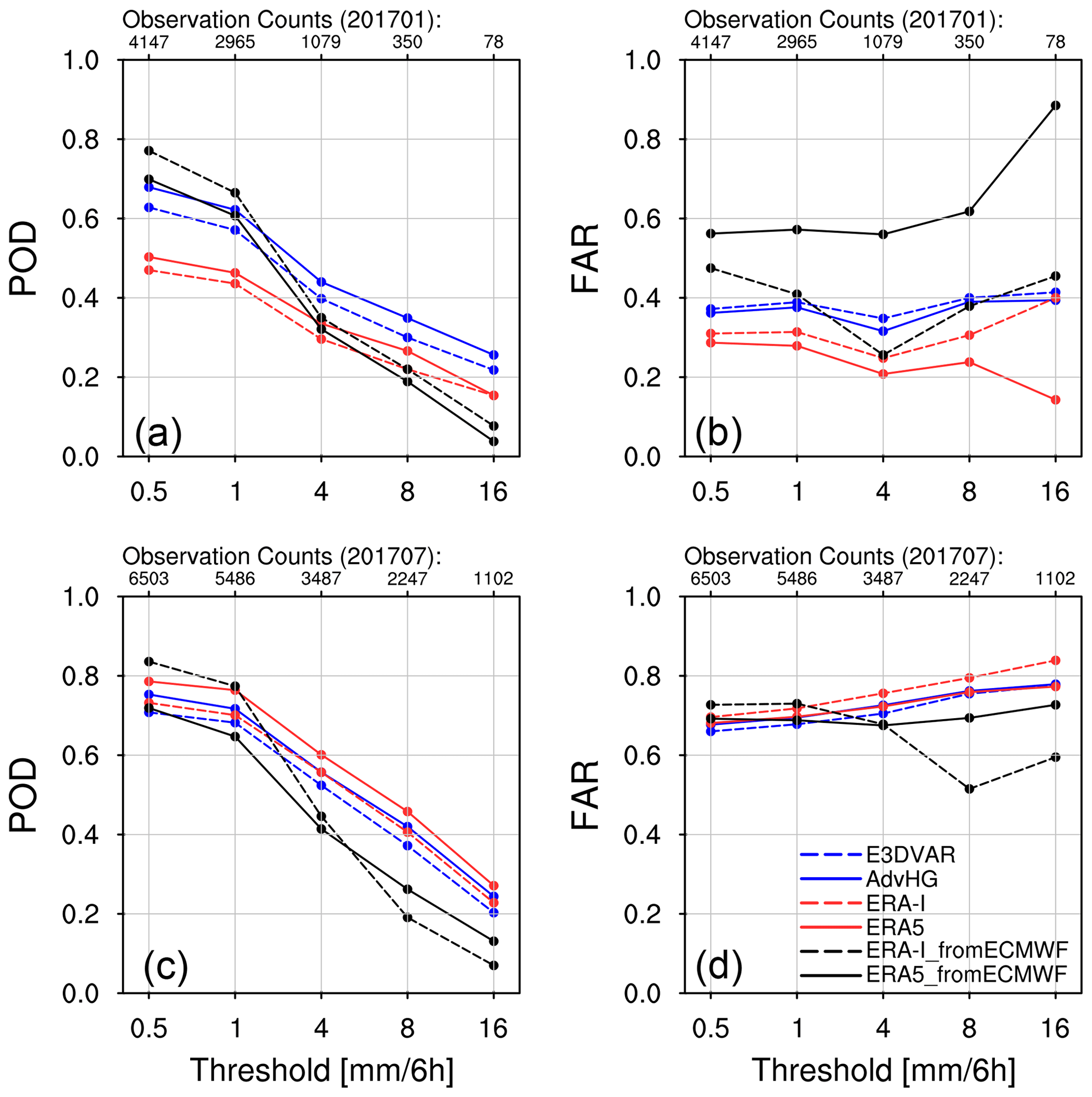
Figure 9 (a, c) POD and (b, d) FAR for (a, b) January and (c, d) July 2017 depending on thresholds 0.5, 1, 4, 8, and 16 mm per 6 h.

For July 2017, generally, AdvHG shows the largest POD, except for ERA5 (Fig. 9c). The FAR values in July are much greater than those in January, which is consistent with the ETS difference between these two seasons.

Brier skill score

The neighborhood sizes are chosen to be 3Δx, 5Δx, 9Δx, and 11Δx, which are 36, 60, 108, and 132 km, respectively, and the thresholds 0.5, 1, 4, 8, and 16 mm per 6 h are considered. The probabilistic precipitation forecasts are calculated at every model grid point depending on neighborhood sizes and thresholds. Regarding each observation, the nearest model grid point to observations is considered as the center of the neighborhood. For verification, 6 h accumulated precipitation fields are extracted from the first 0–6 h forecast fields of WRF-based ERA-I, WRF-based ERA5, E3DVAR, and AdvHG every 6 h (00:00, 06:00, 12:00, and 18:00 UTC). The BSSs of ERA5_fromECMWF and ERA-I_fromECMWF are not calculated, because they have a different resolution from WRF-based results.

Based on the neighborhood approach, the BSS is calculated depending on different neighborhood sizes for January and July 2017, respectively (Fig. 10). Because the reference of BS is chosen as the ERA-I, the positive BSS suggests a better accuracy than ERA-I. In general, for both months, the AdvHG BSS is greater than the ERA5 BSS. Although the E3DVAR BSS is the greatest in July 2017, the AdvHG BSS is the greatest in January 2017.

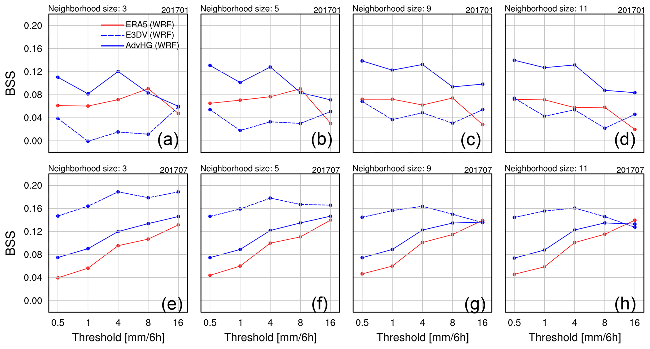
Figure 10 Brier skill score of the probabilistic postprocessed forecast with reference to the WRF-based ERA-I for (a–d) January and (e–h) July 2017 (solid blue line: AdvHG; dashed blue line: E3DVAR; solid red line: WRF-based ERA5).

For January 2017, as a neighborhood size increases, the AdvHG and E3DVAR BSSs tend to increase except for ERA5. Overall, the AdvHG BSS is the greatest among other BSSs for all thresholds for all neighborhood sizes. The ERA5 BSS is greater than the E3DVAR BSS except for 16 mm per 6 h. The highest BSS of AdvHG and the lowest BSS of ERA-I are consistent with the ETS result. Unlike the greater E3DVAR ETS than ERA5 ETS, the ERA5 BSS is greater than the E3DVAR BSS in January 2017.

For July 2017, while the ETS difference between the WRF-based results is not distinct (Fig. 8c), the BSS difference is rather noticeable. Generally, the E3DVAR BSS is the greatest among other BSSs for all thresholds except for 16 mm per 6 h for neighborhood sizes 9 and 11. Although the E3DVAR BSS is the largest, AdvHG outperforms ERA5 and ERA-I. The worst performance of ERA-I precipitation is consistent with the ETS result. At 0.5, 1, and 4 mm per 6 h thresholds, E3DVAR BSS is the greatest, which is similar to ETS. At 8 and 16 mm per 6 h thresholds, ERA5 ETS is the highest, followed by AdvHG and E3DVAR, whereas overall, the E3DVAR BSS is the highest, followed by AdvHG and ERA5.

4.2.2 Spatial distribution

Six h accumulated precipitation with the pattern correlation coefficient

In this section, the spatial distributions of 6 h accumulated precipitation from the WRF-based forecast and reforecast from ECMWF are compared. In addition, pattern correlation coefficients (PCC) are calculated and shown at the bottom right of Figs. 11 and 12.

The PCC is computed according to the usual Pearson correlation operating on the N observed point pairs of 6 h accumulated precipitation fields simulated from (re)forecast and observations at the specific time. For the calculation of PCC, 6 h accumulated precipitation fields from (re)forecast fields are interpolated bilinearly to the N observed points.

First, on 29 and 30 January 2017 (Fig. 11), it is noticeable that the precipitation fields of AdvHG match observations well over East Asia, whereas, in particular, those of ERA5_fromECMWF do not. For example, ERA5_fromECMWF overestimates precipitation over the inland area of China (Fig. 11zz), while AdvHG simulates precipitation similar to observations regarding its position and intensity (Fig. 11x). ERA5_fromECMWF also shows a noticeably smaller PCC (Fig. 11g, n, and zz). Although PCC does not represent the exact accuracy or predictability of precipitation, the overall feature of PCC is consistent with the results found so far. For January 2017, the averaged PCC of AdvHG is the greatest (i.e., 0.61) and that of ERA5_fromECMWF is the smallest (i.e., 0.46; not shown).

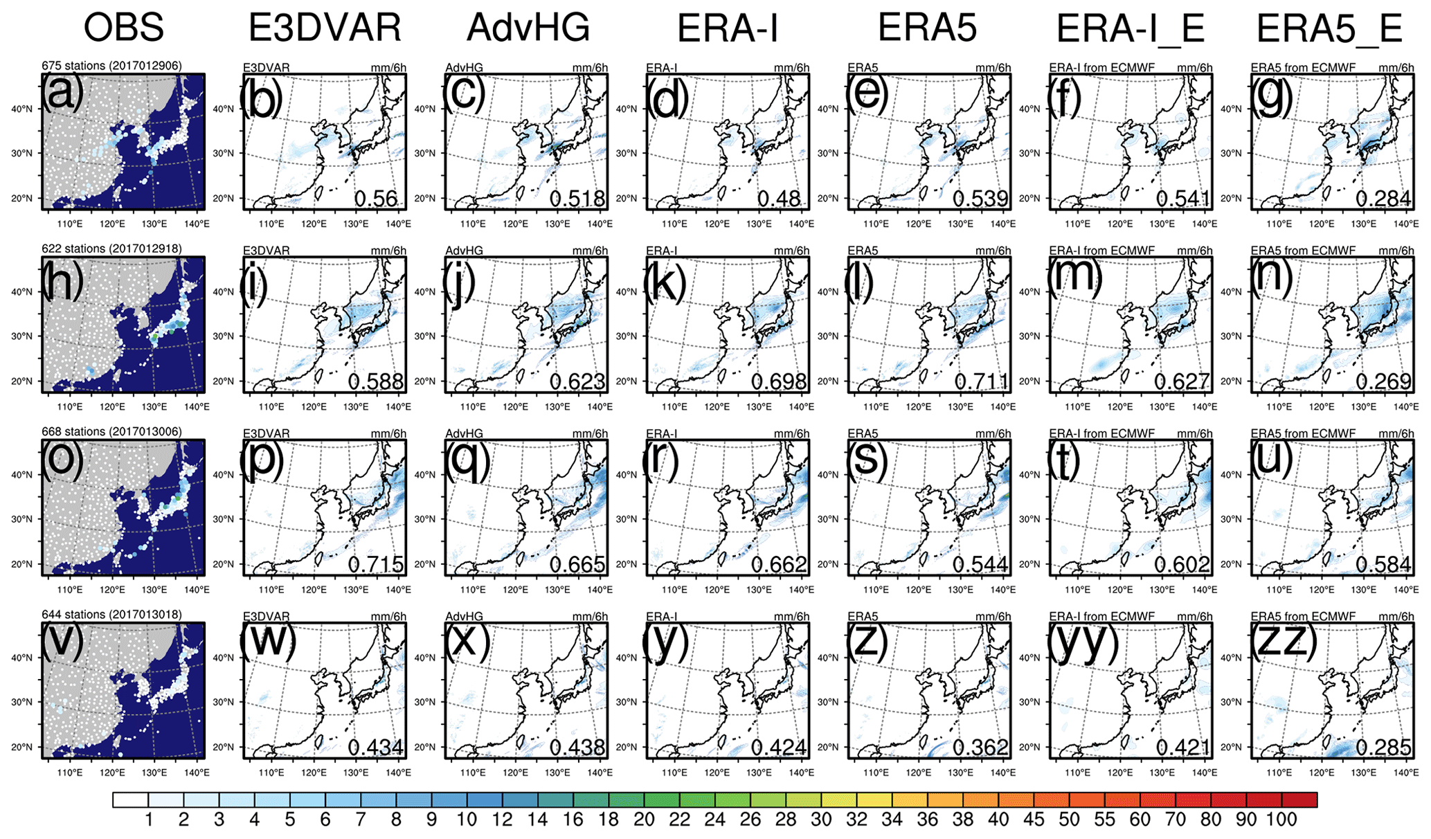
Figure 11 The spatial distribution of 6 h accumulated precipitation of (1st column) observation, (2nd column) E3DVAR, (3rd column) AdvHG, (4th column) ERA-I, (5th column) ERA5, (6th column) ERA-I_fromECMWF, and (7th column) ERA5_fromECMWF and the pattern correlation coefficient (PCC) shown at the bottom right of each figure at the valid time (1st row, 3rd row) of 06:00 UTC and (2nd row, 4th row) 18:00 UTC on 29 and 30 January 2017.​​​​​​​

For 1 and 2 July 2017 (Fig. 12), in general, AdvHG, E3DVAR, and ERA5 simulate well not only the overall features of precipitation fields but also their intensity. During July 2017, ERA5 and ERA-I simulate heavier precipitation than AdvHG (not shown), which is consistent with the larger FBI of ERA5 and ERA-I at higher thresholds. For the 1-month period of July 2017, the averaged PCC of ERA5 is the greatest (i.e., 0.37) and that of AdvHG is 0.34, but the PCC difference between ERA5 and AdvHG is not distinctive. Moreover, the overall range of averaged PCC of different datasets in summer (i.e., 0.29–0.35) is smaller than that in winter (i.e., 0.46–0.61), which is consistent with the seasonal difference of ETS in this study.

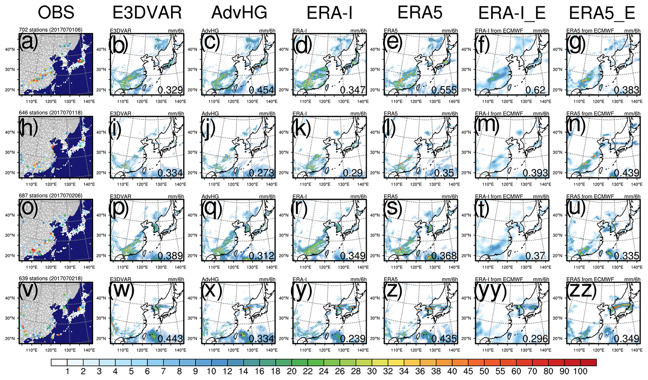
Figure 12 The same spatial distribution of 6 h accumulated precipitation as in Fig. 11, but for 1 and 2 July 2017.

Monthly accumulated precipitation

In this section, the monthly accumulated precipitation fields of rain gauge-based observations, E3DVAR, AdvHG, ERA-I, ERA5, ERA-I_fromECMWF, and ERA5_fromECMWF are compared with each other for two 1-month periods in January and July 2017, respectively.

The monthly accumulated precipitation fields simulated by E3DVAR and AdvHG (Fig. 13b and c) are similar to each other, and E3DVAR and AdvHG produce the best fit to observed fields. Especially for the northwestern part of Japan (e.g., Chugoku and Kinki), E3DVAR and AdvHG are able to represent precipitation correctly, whereas ERA-I_fromECMWF and ERA5_fromECMWF fail to do so (Fig. 13). Moreover, although all the results similarly represent overall features of precipitation in January (Fig. 13), ERA5_fromECMWF (Fig. 13g) simulates the overestimated precipitation over South China, which is consistent with the results in the previous section as well as its larger FBI at lower thresholds (0.5 and 1 mm per 6 h) shown in Fig. 8b. It is noticeable that all results fail to represent the observed precipitation area over the Tibetan Plateau (25–40^∘ N, 95–105^∘ E).

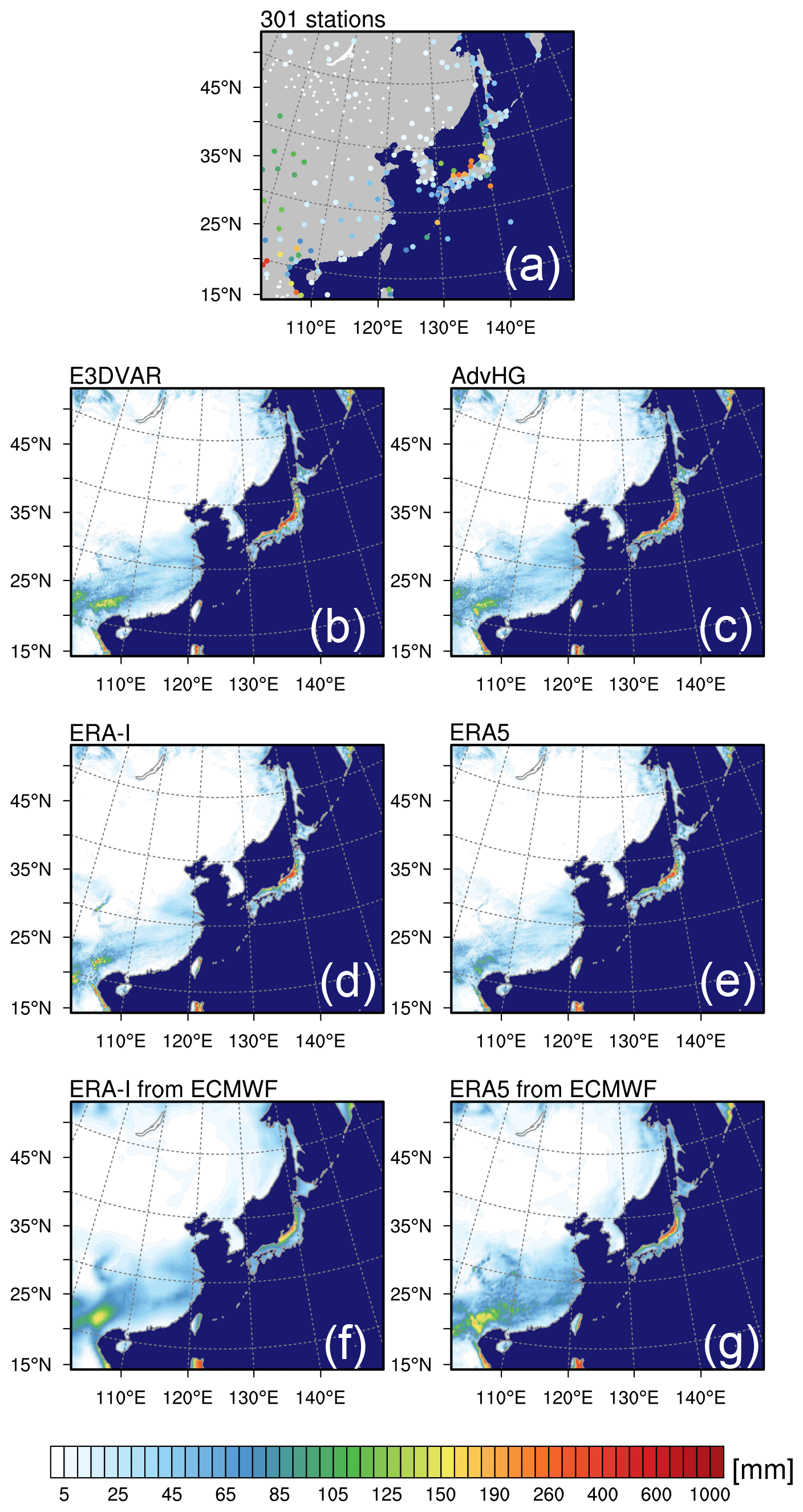
Figure 13 The spatial distribution of the monthly accumulated precipitation of (a) observations, (b) E3DVAR, (c) AdvHG, (d) ERA-I, (e) ERA5, (f) ERA-I from ECMWF, and (g) ERA5 from ECMWF for January 2017.

For the monthly accumulated precipitation in July 2017, overall, the ERA5_fromECMWF (Fig. 14g) and the WRF-based results (Fig. 14b, c, and e) except for ERA-I (Fig. 14d) simulate precipitation well, similar to observations. The WRF-based results including AdvHG overestimate precipitation over the western and southern parts of Japan, while ERA-I_fromECMWF and ERA5_fromECMWF simulate similar precipitation fields to observed fields. The WRF-based results tend to overestimate precipitation in South China, Korea, and Japan, compared with ERA-I_fromECMWF and ERA5_fromECMWF. This is consistent with the result in Fig. 8d, in which FBIs from WRF-based results are generally greater than for higher thresholds (8 and 16 mm per 6 h), whereas those from ECMWF are smaller than 1.

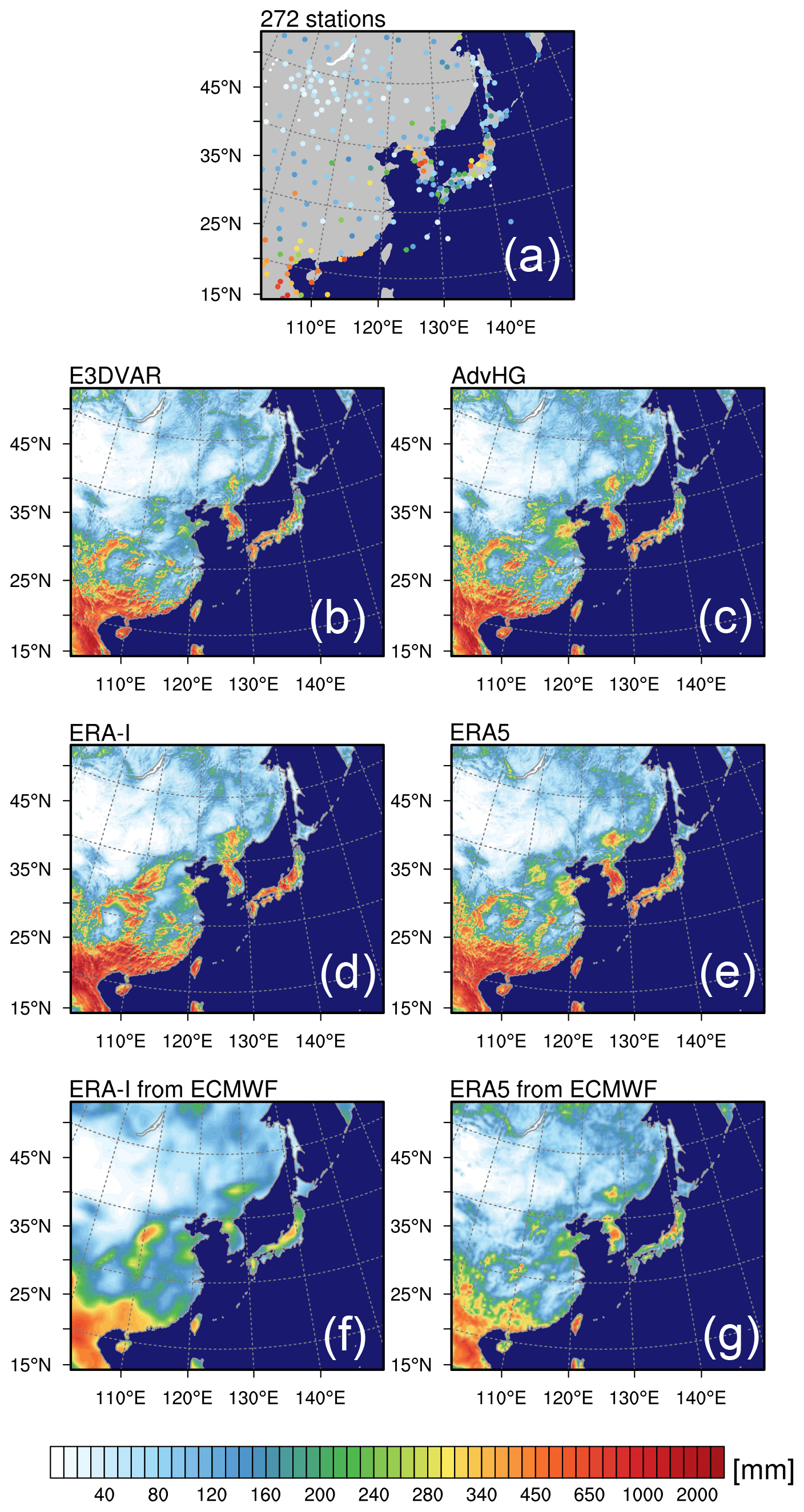
Figure 14 Same observations as in Fig. 13, but for July 2017.

Even though the detailed precipitation features of WRF-based results are different, the overall features of precipitation from WRF-based results are similar to each other, which implies that predictability of precipitation strongly depends on the physics schemes as well as on the NWP model, especially for the summer season. According to Que et al. (2016), depending on the combinations of physics options in the WRF model, the spatial distribution of precipitation can be significantly different over the Asian summer monsoon area, and the YSU PBL scheme which is used in this study tends to overestimate precipitation over the same area. Thus, different physics options could simulate the different spatial distribution of precipitation.

In addition, compared to ERA5 based on the WRF model (Fig. 14e), the ECMWF model for ERA5_fromECMWF (Fig. 14g) seems to suppress precipitation. Thus, the WRF model with the physics schemes used in this study might simulate more precipitation than the ECMWF model, although the initial condition is the same. Therefore, it is important to consider the consistency of the systems for DA and the forecast model for a good performance of forecast weather variables such as precipitation.

5 Data availability

The EARR data presented in this study are available every 6 h (i.e., 00:00, 06:00, 12:00, and 18:00 UTC) for the period 2010–2019 from the Harvard Dataverse Repository (https://dataverse.harvard.edu/dataverse/EARR, last access: 17 March 2022). The EARR 6 hourly data on pressure levels (https://doi.org/10.7910/DVN/7P8MZT, Yang and Kim, 2021b) and 6 hourly precipitation data (https://doi.org/10.7910/DVN/Q07VRC, Yang and Kim, 2021c) are provided in NetCDF file format.

The EARR 6 hourly data on pressure levels (Yang and Kim, 2021b) include u-component of wind, v-component of wind, temperature, geopotential height, and specific humidity variables of reanalysis on pressure levels (i.e., 925, 850, 700, 500, 300, 200, 100, and 50 hPa). The EARR 6 hourly precipitation data (Yang and Kim, 2021c) contain the 6 h accumulated total precipitation variable of the 6 h reforecast on a single level. The 6 h accumulated total precipitation is obtained from the 6 h reforecast field which is integrated for 6 h from the reanalysis field every 6 h (i.e., 00:00, 06:00, 12:00, and 18:00 UTC).

6 Summary and conclusions

In this study, to develop the regional reanalysis system over East Asia, the advanced hybrid gain algorithm (AdvHG) is newly proposed and evaluated with a traditional hybrid DA method (E3DVAR) as well as existing reanalyses from ECMWF (ERA5 and ERA-I) for January and July 2017. The East Asia Regional Reanalysis (EARR) system is developed based on the AdvHG as the data assimilation method using the WRF model and conventional observations. The high-resolution regional reanalysis and reforecast fields over East Asia with 12 km horizontal resolution are produced and evaluated against observations with ERA5 for the 10-year period 2010–2019.

The AdvHG newly proposed in this study is based on the hybrid gain approach, weighting analyses from variational-based and ensemble-based DA algorithms to generate optimal hybrid analysis, which can play an important role as a simple and practical method in the foreseeable future to take advantage of the strength of each DA method. The advanced hybrid gain method is different from the hybrid gain approach in that (1) E3DVAR is used instead of EnKF, (2) 6 h forecast of ERA5 is used instead of deterministic analysis for a more balanced and consistent analysis with the WRF model, and (3) the pre-existing and state-of-the-art reanalysis data (i.e., ERA5) are simply used instead of producing our own analysis fields from a variational DA method. Thus, it can be regarded as an efficient approach for generating a regional reanalysis dataset because of cost savings and the use of the state-of-the-art reanalysis from ECMWF that assimilates all available observations.

For verification, the latest ECMWF reanalysis and reforecast datasets (i.e., ERA5 and ERA-I) are used. With respect to forecast variables, two different forecast fields of ECWMF are used: (1) reforecast fields from ECMWF (i.e., ERA5_fromECMWF and ERA-I_fromECMWF) and (2) forecast fields (i.e., WRF-based ERA5 and WRF-based ERA-I) integrated in the WRF model with 12 km resolution using ERA5 and ERA-I as initial conditions.

Analysis and forecast wind, temperature, and humidity variables of AdvHG are evaluated with ERA5 for the 10-year period and assessed with five different experiments (i.e., E3DVAR, ERA5, ERA-I, ERA5_fromECMWF, ERA-I_fromECMWF) for January and July 2017. Overall, the analysis RMSE of E3DVAR is the smallest among others but comparable to that of ERA5, especially for January 2017. Regarding forecast variables, AdvHG outperforms E3DVAR for January and July 2017. Although ERA5 outperforms AdvHG for upper-air variables for two seasons in 2017, AdvHG outperforms ERA-I in January and shows comparable performance to ERA-I in July. Additionally, the verification results of AdvHG and ERA5 for the period 2010–2019 are consistent with those for two 1-month periods in 2017.

The precipitation forecast variables are also verified regarding a neighborhood-based verification score (i.e., BSS) as well as the point-based verification scores (i.e., ETS, FBI, POD, and FAR). According to the point-based verification scores, the precipitation forecast of AdvHG in January is the most accurate, followed by E3DVAR, ERA5, and ERA-I. For July, the overall ETS values of all results are relatively lower than those in January, implying a lower predictability in summer. In addition, the ETS differences between the results are not distinctive in July. For higher thresholds (8 and 16 mm per 6 h) in July, AdvHG ETS is greater than E3DVAR ETS and smaller than ERA5 ETS, whereas E3DVAR ETS is the greatest followed by ERA5 and AdvHG for lower thresholds (0.5 and 1 mm per 6 h).

To prevent double penalty when verifying highly variable data with high resolution (e.g., precipitation), the BSS based on the neighborhood approach is calculated for 6 h accumulated precipitation forecasts depending on different neighborhood sizes for January and July 2017. In general, the BSS of AdvHG is greater than that of ERA5 and ERA-I for both months. Although the E3DVAR BSS is the greatest in July 2017, the AdvHG BSS is the greatest in January 2017.

Lastly, the spatial distributions of 6 h and monthly accumulated precipitation forecast for AdvHG, E3DVAR, ERA-I, ERA5, ERA-I_fromECMWF, and ERA5_fromECMWF are compared with rain gauge-based observations. For January 2017, it is noticeable that AdvHG precipitation is the closest to observations with the highest PCC (i.e., 0.61), and ERA5_fromECMWF overestimates precipitation over South China with the lowest PCC (i.e., 0.46). For July 2017, the WRF-based results tend to overestimate precipitation compared to ERA-I_fromECMWF and ERA5_fromECMWF. In addition, even though the averaged PCC of ERA5 (i.e., 0.37) is slightly greater than that of AdvHG (i.e., 0.34), the PCC difference between ERA5 and AdvHG is not distinctive and overall the range of averaged PCC of all datasets in summer (i.e., 0.29–0.37) is smaller than that in winter (i.e., 0.46–0.6).

In conclusion, for upper-air variables, overall, ERA5 outperforms EARR based on AdvHG, but the RMSE difference between ERA5 and EARR (AdvHG) is smaller than that between ERA5 and ERA-I. In addition, EARR outperforms ERA-I for January 2017 and shows comparable performance to ERA-I for July 2017. On the contrary, according to the evaluation results of precipitation, in general, EARR represents precipitation better than ERA5 as well as ERA5_fromECMWF for January and July 2017. Even if E3DVAR precipitation is better represented than EARR precipitation for July, the difference is not considerable for July and EARR simulates precipitation for January better than E3DVAR does. Therefore, although the uncertainties of upper-air variables of EARR should be considered when analyzing them, the precipitation reforecast of EARR is more accurate than that of ERA5 for both seasons.

Combining the global reanalysis data (i.e., ERA5) characterized by the high quality of large-scale features with detailed smaller-scale features in the higher resolution represented by the ensemble-based assimilation method (i.e., E3DVAR) as well as a community numerical weather prediction model (i.e., WRF model) is a key factor for EARR to be able to produce high-resolution initial conditions represented with regional features, which could contribute to a reduction in forecast errors, especially for precipitation. Therefore, EARR has its own advantage of representing regional features of precipitation better than relatively coarse-resolution global reanalysis.