the Creative Commons Attribution 4.0 License.
the Creative Commons Attribution 4.0 License.
 | 27 Apr 2022
EUREC4A observations from the SAFIRE ATR42 aircraft
Marie Lothon
Julien Delanoë
Pierre Coutris
Jean-Claude Etienne
Franziska Aemisegger
Anna Lea Albright
Thierry André
Hubert Bellec
Alexandre Baron
Jean-François Bourdinot
Pierre-Etienne Brilouet
Aurélien Bourdon
Jean-Christophe Canonici
Christophe Caudoux
Patrick Chazette
Michel Cluzeau
Céline Cornet
Jean-Philippe Desbios
Dominique Duchanoy
Cyrille Flamant
Benjamin Fildier
Christophe Gourbeyre
Laurent Guiraud
Tetyana Jiang
Claude Lainard
Christophe Le Gac
Christian Lendroit
Julien Lernould
Thierry Perrin
Frédéric Pouvesle
Pascal Richard
Nicolas Rochetin
Kevin Salaün
Alfons Schwarzenboeck
Guillaume Seurat
Bjorn Stevens
Julien Totems
Ludovic Touzé-Peiffer
Gilles Vergez
Jessica Vial
Leonie Villiger
Raphaela Vogel
As part of the EUREC4A (Elucidating the role of cloud–circulation coupling in climate) field campaign, which took place in January and February 2020 over the western tropical Atlantic near Barbados, the French SAFIRE ATR42 research aircraft (ATR) conducted 19 flights in the lower troposphere. Each flight followed a common flight pattern that sampled the atmosphere around the cloud base level, at different heights of the subcloud layer, near the sea surface and in the lower free troposphere. The aircraft's payload included a backscatter lidar and a Doppler cloud radar that were both horizontally oriented; a Doppler cloud radar looking upward; microphysical probes; a cavity ring-down spectrometer for water isotopes; a multiwavelength radiometer; a visible camera; and multiple meteorological sensors, including fast rate sensors for turbulence measurements. With this instrumentation, the ATR characterized the macrophysical and microphysical properties of trade-wind clouds together with their thermodynamical, turbulent and radiative environment. This paper presents the airborne operations, the flight segmentation, the instrumentation, the data processing and the EUREC4A datasets produced from the ATR measurements. It shows that the ATR measurements of humidity, wind and cloud base cloud fraction measured with different techniques and samplings are internally consistent; that meteorological measurements are consistent with estimates from dropsondes launched from an overflying aircraft (the High Altitude and LOng Range Research Aircraft, HALO); and that water-isotopic measurements are well correlated with data from the Barbados Cloud Observatory. This consistency demonstrates the robustness of the ATR measurements of humidity, wind, cloud base cloud fraction and water-isotopic composition during EUREC4A. It also confirms that through their repeated flight patterns, the ATR and HALO measurements provided a statistically consistent sampling of trade-wind clouds and of their environment. The ATR datasets are freely available at the locations specified in Table 11.
- Article
(24641 KB) - Full-text XML
- BibTeX
- EndNote


The interaction of trade-wind clouds with their environment is at the center of fundamental questions such as the role of clouds in climate sensitivity. The EUREC4A field campaign, which took place in January–February 2020 near Barbados, has been designed specifically to address this issue (Bony et al., 2017). During 1 month, four research aircraft, four research vessels, ground-based observations and a myriad of autonomous observing systems characterized clouds and the environment surrounding them over a large range of space scales (Stevens et al., 2021). To elucidate the couplings between clouds and circulation, the nucleus of the experimental strategy was based on the coordinated and repeated flight plans of two core platforms: HALO (High Altitude and LOng Range Research Aircraft, operated by the German Aerospace Center; Konow et al., 2021) and the ATR-42 (hereafter referred to as ATR), operated by the French Service des Avions Français Instrumentés pour la Recherche en Environnment (SAFIRE). These airborne operations were augmented with other platforms operating within the same area, including the Twin Otter operated by the British Antarctic Survey (Denby et al., 2022), the P-3 aircraft operated by the NOAA (Pincus et al., 2021), a Barbadian aircraft operated by the Regional Security System (RSS), the BOREAL and Skywalker unmanned aerial vehicles (UAVs) operated by Météo-France, and the CU-RAAVEN UAV operated by the University of Colorado (de Boer et al., 2022). In addition, ground- and ship-based observations from the Barbados Cloud Observatory (BCO; Stevens et al., 2016) and a research vessel (R/V Meteor) were continuously documenting the atmospheric state on the western and eastern sides of the ATR operations area, respectively.
While HALO was flying at an altitude near 10 km to observe the cloud field from above and to document the environment of clouds with dropsondes, the ATR was flying in the lower troposphere to characterize clouds and their environment through in situ and remote sensing measurements. To help understand the physical processes that control the climate change cloud feedbacks and the mesoscale organization of shallow convection, the primary mission of the ATR was to measure the cloud fraction near cloud base and the dynamical and thermodynamical environment of clouds from the turbulent scale to the mesoscale (Bony et al., 2017).
Due to the nature of the trade-wind regimes, fulfilling this mission constitutes an experimental challenge. First of all, the cloud field in these regimes is composed of very small and thin broken clouds, with an expected cloud fraction at cloud base of only a few percent. Accurate measurements of the cloud base cloud fraction therefore require both a good sensitivity of the instruments to the presence of clouds and an adequate sampling of the cloud field. Secondly, the humidity field is associated with extremely large and steep vertical gradients, ranging from 80 % near the surface to 100 % within clouds and to less than 5 % above the trade inversion (Stephan et al., 2021). These gradients favor phase changes and the deposition of cloud droplets on airborne sensors, which can affect the response time and accuracy of the measurements.
These challenges were met by fitting the aircraft with a wealth of instrumentation, which, in some cases, was used in an airborne configuration for the very first time. The instrumentation was also chosen to promote redundancy or complementarity of sensors and measurement techniques. This redundancy was not only important for the post-processing and calibration of the data, it was also essential to assess the robustness of the ATR measurements of cloud fraction, humidity and winds.
The goal of this paper is to provide an overview of the operations and measurements of the ATR during EUREC4A. Section 2 presents the aircraft, the operations, the flight patterns and their segmentation, and the weather conditions during the flights. Section 3 presents the ATR instrumentation, ranging from the core instrumentation of the aircraft to the instruments that were specifically devised for EUREC4A and provides a brief description of the data post-processing and of the associated datasets. The focus is put on the datasets which have not been subject to specific data papers. Section 4 assesses the internal consistency of ATR measurements regarding the cloud base cloud fraction, humidity and wind, and their consistency with observations from other platforms. Links to the data are provided in Sect. 5, and a brief summary and conclusions are presented in Sect. 6.
2.1 A challenging start
The SAFIRE ATR42 (F-HMTO) is a turbo-propeller aircraft flying in the lower troposphere (its ceiling is at about 7.5 km) which has been modified in many ways to fit scientific research purposes. The preparation of the ATR for the EUREC4A campaign was associated with significant challenges.
First of all, the ATR home base is in Toulouse (in the south of France), and to join the Caribbean during boreal winter, the aircraft had to follow the historical route of the Aerospostale through Tenerife (Canary Islands), Prahia (Cape Verde) and Fortaleza (Brazil). As the crossing of the Atlantic Ocean required an exceptionally long flight (8 h) compared to the maximal autonomy of the aircraft (8.5 h), the ATR had to be kept as light as possible during the transit. For this purpose, most of the EUREC4A instruments and aircraft equipment had to be unmounted from the ATR in Toulouse and shipped to Barbados well in advance of the transit. The final segment from Fortaleza and Barbados was also at the limit of the aircraft autonomy. Unfavorable wind conditions imposed a refuel in Cayenne (French Guyana), but the ATR finally landed in Barbados 5 d after its departure from Toulouse. It was the most remote campaign ever accomplished by this aircraft.
Second, extraordinary circumstances independent of SAFIRE and EUREC4A considerably delayed the maintenance and the upgrade of the aircraft avionics during the last months before the campaign. As a result, and for the first time in SAFIRE history, the full integration of the campaign's scientific payload into the aircraft could not take place in Toulouse as planned but had to be accomplished on site. Most of the aircraft equipment and scientific instruments were mounted on the aircraft after the ATR landed in Barbados on 19 January, and the whole EUREC4A payload flew for the first time in the ATR during the electromagnetic interference (EMI) flight, which took place in Barbados on 23 January. Although the EMI test was successful, this first flight with the whole EUREC4A instrumentation revealed a number of problems that had to be fixed. Therefore, the ATR did not participate in the first coordinated flight of the EUREC4A campaign on 24 January but planned another test flight on 25 January (RF02), including special maneuvers for calibration purposes, and started coordinated missions with the other aircraft on 26 January. On 26 January unfortunately, the inertial navigational system (INS) of the scientific instruments showed malfunctioning. A solution was found, requiring however that for the rest of the campaign, the acquisition rate of navigation data be recorded at 50 Hz instead of 100 Hz.
Despite these challenges to prepare the aircraft for the campaign, the ATR conducted 19 research flights on 11 operation days from 25 January to 13 February 2020 (totaling approximately 82 flight hours; Table 1) and successfully fulfilled the scientific mission that it aimed to accomplish.
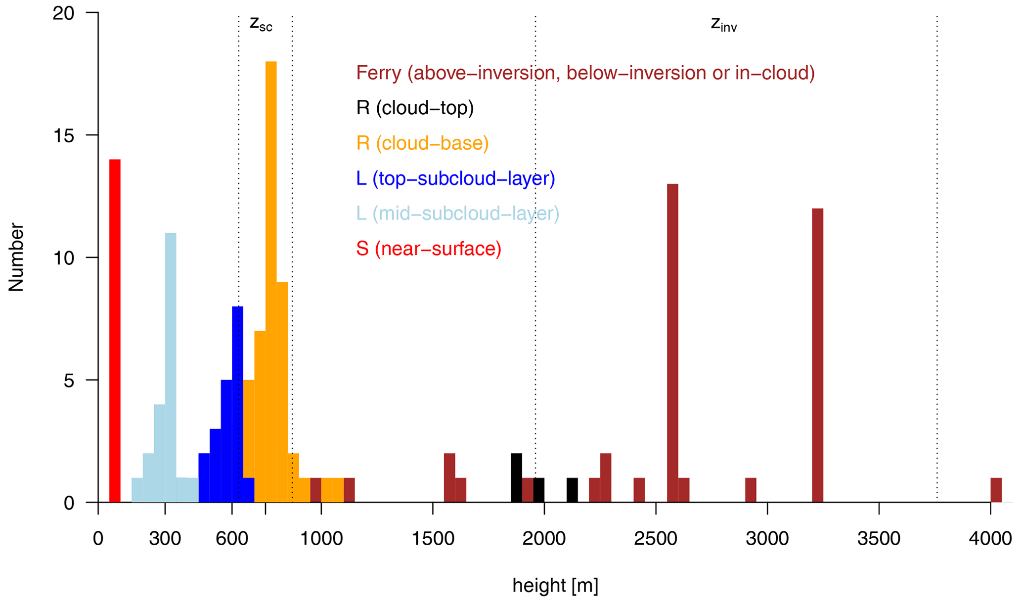
Table 1 List of ATR flights with a brief description of the main flight patterns: the mean approximate height (and number) of rectangles flown around cloud base (Rb) or cloud top (Rt), the height of the L patterns flown near the top and the middle of the subcloud layer, the height of the near-surface leg (S pattern) and of the ferry legs flown above clouds.
1 On 30 January 2020, from 11:42 to 12:32 UTC, HALO flew two racetrack patterns above the ATR rectangle. 2 On 9 February 2020, from 14:32 to 17:00 UTC, the ATR flew within the field of view of the RSS aircraft. 3 On 11 February 2020, from 04:17 to 07:25 UTC, the P3 flew two circular patterns within the EUREC4A circle at an altitude of about 7.5 km and dropped 12 sondes along its first circle (from 04:17 to 05:55 UTC) just before the ATR takeoff.
2.2 Flight patterns
The ATR generally performed two flights per day in coordination with the other aircraft. Each research flight was typically 4.5 or 5 h long, including a transit time from the airport to the EUREC4A circle of about 20 min in each direction. The refuel in Barbados between two flights was about 1 h long so that within 90 min, the ATR was back in the measurement zone for a second mission (Table 1). While the ATR was flying in the lower troposphere, HALO was observing the cloud field from aloft and was dropping sondes along three consecutive circles of about 200 km diameter (Konow et al., 2021).
The ATR's mission was primarily focused on characterizing the cloud base cloudiness, subcloud-layer properties and their signals of spatial organization at the turbulent scale and at the mesoscale. For this purpose, each flight was composed of a basic set of patterns near cloud base and within the subcloud layer that were repeated independent of meteorological conditions. This repetition was motivated by the wish to sample the diversity of boundary layer conditions without any bias and to compare the flights with each other. Then, depending on flight and weather conditions, a few additional patterns were flown near cloud top, at cloud base and/or near the sea surface. Owing to the sharp vertical humidity gradients of the atmosphere and the need to minimize the instruments' memory effects, and due to the abundant presence of sea salt near the ocean surface, which can dirty the instruments'optics, the patterns were preferentially flown from top to bottom.
Figure 2(a) Longitude–latitude trajectories of the ATR colored by the flight altitude (for repetitive flight patterns such as the rectangles, only the last repetition is visible due to overlap). The dashed circle represents the EUREC4A circle. The ATR track is shown for RF11 (5 February) on top of a satellite snapshot of the domain (11.8–14.8∘ N, 57–60∘ W) derived from the visible channel of GOES-16 at about mid-flight time (the tracks of all other flights are shown in Fig. ). (b) Three-dimensional representation of the ATR trajectory during the same flight (RF11), colored by the relative humidity measured at the flight level.
Shortly after takeoff, the ATR ferried towards the EUREC4A circle generally at an altitude of 2.5, 3.5 or 4.5 km, so above or around the trade inversion level (Fig. 2). Upon arrival over the measurement area, it started to fly large rectangles (or racetrack patterns, also referred to as “R patterns”) of about 120 km × 20 km, perpendicular to the mean easterly wind. The width of the rectangle was chosen so as to best sample the cloud field within the rectangle area using horizontal lidar–radar measurements (Sect. 3.5.3). At least two rectangles were flown around cloud base (around 750 m), at an altitude determined with the help of the ground-based support (Sect. 2.3). When an extensive stratiform cloud layer was present near the trade inversion level (as during RF11, RF13, RF17 and RF19), the ATR could fly an additional rectangle around cloud top (near 2 km). Otherwise it flew an additional rectangle at cloud base to increase the cloud base sampling. The flight trajectories and patterns associated with each flight are shown in Figs. and .
Figure 3Schematic representation of the trade-wind layer with the different levels considered as part of the ground support to determine the cloud base level of the ATR, plus sometimes the cloud top level. The subcloud-layer top, referred to as h or zSC, is defined as the level of neutral buoyancy of a parcel originating from the surface layer with a 0.2 K excess in θv (Sect. 2.5); zCFmax is the level of maximum near-base cloud fraction (as would be seen for instance in ground-based radar observations), cbhceil is the peak of the distribution of the first-detected cloud base height (cbh) of the ceilometer, zRHmax is the level of maximum relative humidity (RH) at the mixed-layer top, LCL is the lifting condensation level, zinv,RH and are the inversion heights based on the maximum gradients in RH and θv, and zCFinv is the second level of maximum cloud fraction around the inversion.
Then, to characterize the turbulent and mesoscale organization of the subcloud layer, the ATR flew two L-shape patterns within the subcloud layer, one near the top of the subcloud layer (generally around 600 m) and the other near the middle of the subcloud layer (around 300 m). As the organization of the boundary layer can be anisotropic and dependent on the wind direction, each L pattern was composed of two straight legs perpendicular to each other (each leg being about 60 km long): one along-wind and one cross-wind. Finally, in daylight conditions a near-surface leg of about 40 km was performed at an altitude of about 60 m before returning to the Grantley Adams International Airport (BGI) in Barbados through another ferry leg in the free troposphere.
A few flights were associated with particular features:
-
During RF06 (30 January), from 11:42 to 12:32 UTC, HALO flew (twice as fast as the ATR) two racetrack patterns above the ATR rectangle at an altitude of about 10 km; two dropsondes were dropped at the extremities of the HALO racetrack. This coordinated flight will help compare the cloud detection and characterization performed with the HALO and ATR measurements.
-
During RF16 (9 February), the ATR flew within the field of view of the RSS aircraft, which was flying parallel to the ATR at about the same altitude. On this occasion, the ATR flew four rectangles around cloud base. The coordination between the two aircraft will help compare the cloud detection performed with the ATR instruments with the high-resolution pictures taken by the visible camera of the RSS aircraft.
-
During RF17 (13 February), the ATR flew during nighttime. This flight was coordinated with the P-3 aircraft (Pincus et al., 2021), which dropped sondes (from an altitude of about 7.5 km) along the EUREC4A circle right before the ATR takeoff.
2.3 Ground support
The main role of the ATR during EUREC4A was to measure the cloud fraction and the thermodynamical, dynamical and microphysical properties of the atmosphere at the interface between the subcloud layer and the cloud layer (Bony et al., 2017; Stevens et al., 2021). A ground crew estimating cloud base height using real-time observations from several observing platforms near and within the targeted flight area provided tactical support for each flight mission. It advised the flight planning about the cloud base level and about the relevance of flying at the top of the cloud layer when an extensive layer of stratiform cloudiness was present near the trade inversion.
As illustrated by Fig. 3, the targeted cloud base level was not the lifting condensation level (LCL) but the height of the maximum near-base cloud fraction (zCFmax). This level corresponds to the level where most clouds in the sampling area have reached their base level, and it is most adequately defined by the height at which a cloud radar reports a maximum cloudiness near cloud base. The cloud base height distributions from the ceilometer and estimates of the mixed-layer top, subcloud-layer top (h) and LCL from soundings and surface weather data provided further guidance for choosing the correct cloud base level.
The evening before the flight, and again 2 h before takeoff, a pre-flight estimation of the flight levels was performed based on near-real-time cloud radar, ceilometer, radiosonde and surface weather data from the BCO and R/V Meteor as well as satellite imagery from the Geostationary Operational Environmental Satellite GOES-16 Advanced Baseline Imager (https://doi.org/10.7289/V5BV7DSR, GOES-R, 2017).
During the flights, real-time ATR lidar backscatter quick-looks and visual impressions from the pilots, as well as real-time information from the HALO dropsondes and lidar quick-looks (Konow et al., 2021), were used to fine-tune the flight level. To provide spatial context between the east–west anchor points (R/V Meteor on the eastern side and BCO on the western side), satellite imagery and HALO data were used to anticipate horizontal gradients in the levels. In case the cloudiness was associated with very shallow clouds, and the cloud base height was exhibiting strong gradients across the sampling area, a slight adjustment in the cloud base flight level along the rectangle or in between subsequent rectangles was allowed to improve the sampling of clouds. Occasionally, the cloud base level was slightly adjusted between the northern and southern halves of a given rectangle. However it was never adjusted between the eastern and western sides of the rectangle so that the cloud field within the rectangle was sampled at the same height by the horizontal lidar–radar measurements performed from opposite sides of the rectangle (see Chazette et al., 2020, for an illustration of the sampling by horizontal lidar measurements).
At the beginning of the last rectangle of each flight, the level of the L patterns to be flown within the subcloud layer was determined. The first L pattern was flown near the top of the subcloud layer, about 150–200 m below the lowest cloud base leg (to make sure no cloud is present), and the second L pattern was flown near the middle of the subcloud layer. Finally, shortly before the ferry back to Barbados and when daylight was still present, the ATR flew short straight legs near the sea surface (S pattern).
Over the campaign, the cloud base flight level ranged from about 600 to 850 m; the L pattern near the top and the middle of the subcloud layer were flown around 500–600 and 200–400 m, respectively; and S patterns were flown about 60 m above the sea surface (Table 1, Fig. 4).
Table 2 Segmentation of the ATR flights into patterns (“kind”), flown at different levels (“note”). Each segment is associated with a “name”, where (N being the number of patterns of the “kind” category flown during the flight); X= A, B, C.... and x= a, b … h. See Fig. 6 for an illustration of the sub-segmentation of the patterns into T-shortlegs, T-longlegs and T-longestlegs segments. Also reported is the total number of segments in each category. This information is included in a set of YAML files (one file per flight).

2.4 Flight segmentation
To aid in the analysis of the flight data, each flight is segmented into non-exclusive timestamps summarized in a set of Yet Another Markup Language (YAML) files (Table 2). Different kinds of segments are defined that correspond to basic patterns (“R pattern”, “L pattern”, “S pattern”) or to particular phases of the flight (e.g., “ferry”). The vertical level at which these patterns are flown (at cloud top, cloud base, near the top of the subcloud layer, near the middle of the subcloud layer, near the sea surface, above or below the trade inversion level) is also indicated as a “note” in the YAML files. The vertical excursions of the ATR are referred to as “profiles”, and the direction (upward or downward) in which they were realized is also reported. An example of flight segmentation is shown for RF11 (Fig. 5). The vertical and horizontal trajectories of each flight are shown in Figs. and .
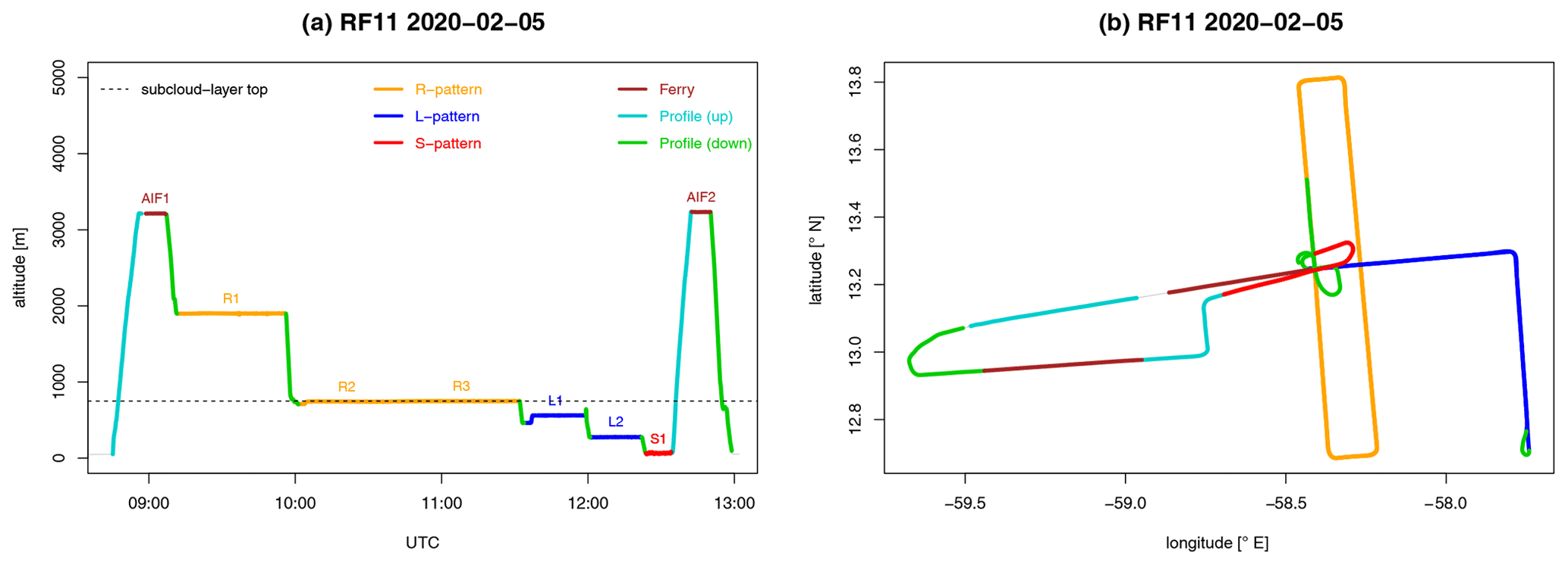
Figure 5(a) Time–height trajectory and (b) longitude–latitude trajectory of the ATR during RF11 (5 February 2020), illustrating the different patterns and segments of the flight. Also reported is the subcloud-layer top diagnosed from HALO dropsondes (Table 3).
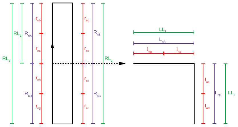
Figure 6Segmentation of the R and L patterns into straight and stabilized segments of equal duration and length for turbulence studies (T-shortlegs: 30 km/5 min in red, referred to as rnx or lnx, where n is the pattern number; T-longlegs: 60 km/10 min in purple, referred to as RnX or LnX). Also reported are the longest stabilized legs in one direction (T-longestlegs, 120 km/20 min or 60 km/10 min, in green, referred to as RLi or LLi, where i=1…P, and P is the number of such segments for the flight). A similar nomenclature is used for the segmentation of the S patterns. See Table 2 for the definition and the nomenclature of these segments. After Brilouet et al. (2021).
The characterization of the turbulence (“T”) requires the consideration of straight and stabilized legs of at least 30 km (Lenschow et al., 1994). For this reason, the R and L patterns were also associated with a finer segmentation in straight horizontal legs of equal duration and length (Fig. 6 from Brilouet et al., 2021): short segments of approximately 30 km (5 min flight) are referred to as “T-shortlegs”, and longer segments of approximately 60 km are referred to as “T-longlegs”. The longest stabilized segments in one direction are also reported as “T-longestlegs”; in contrast with the “T-shortlegs” or `T-longlegs”, these segments can have various lengths, ranging from 60 to 125 km.
Table 3Meteorological conditions associated with each ATR flight and their average over all flights. All quantities are computed from the JOANNE dropsonde dataset (George et al., 2021) as averages over three consecutive circles flown during each ATR flight; zINV, zSC and zLCL are the trade inversion height, the subcloud-layer top height and the lifting condensation level height, respectively; zINV is defined as the height where the moist static energy is minimum between 1300 and 4000 m; zSC is defined as the lowest altitude above 200 m where θv(z) exceeds the mass-weighted average of θv from 200 m to z by more than 0.2 K (Canut et al., 2012; Rochetin et al., 2021; Touzé-Peiffer et al., 2022); zLCL is diagnosed as , with , where T is the temperature and RH the relative humidity. ω is the vertical velocity measured at the scale of the EUREC4A circle by dropsondes (Bony and Stevens, 2019; George et al., 2021); ωSC and ωINV are the mass-weighted averages of ω in a 200 m layer centered around zSC and zINV, respectively. ωFT and RHFT (FT referring to the lower free troposphere) are the mass-weighted averages between 4000 and 6000 m of ω and RH, respectively (note that ω was not measured during RF06). PW (precipitable water) is the mass-weighted integral of water vapor specific humidity from the surface to the altitude of the dropsonde launch (about 10 km). The lower-tropospheric stability (LTS) is defined as LTS (Klein and Hartmann, 1993). Vs is the near-surface wind speed computed from the zonal and meridional wind components measured by dropsondes at 20 m. NA – not available.
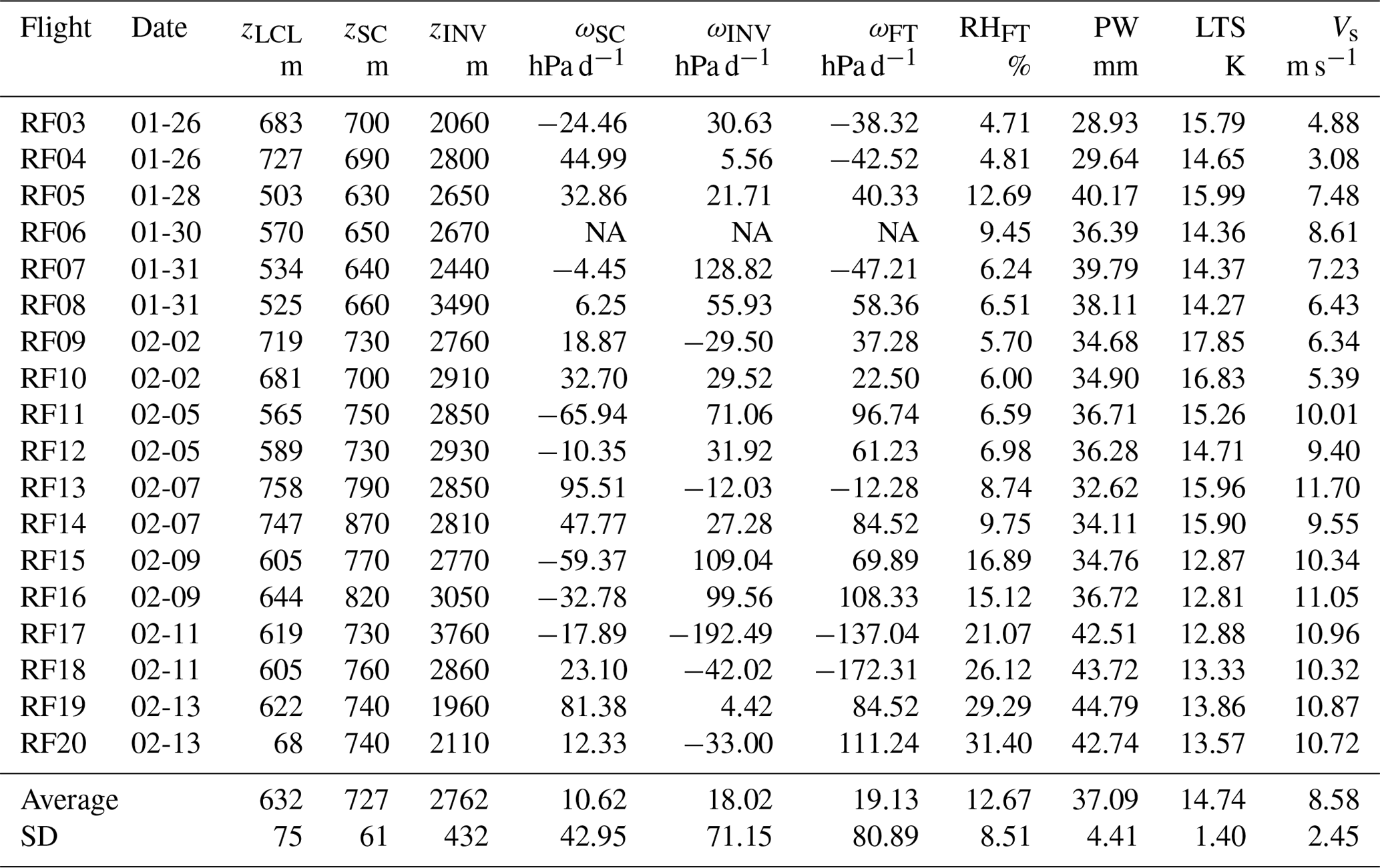
Table 4Cloud, aerosol and precipitation conditions associated with ATR flights. Through the combined analysis of Fig. , GOES-E animations (Appendix B), BCO radar information and C3ONTEXT results (Schulz, 2022), the prominent low-level cloud types (at the scale of the R and L patterns) and cloud mesoscale patterns (at the scale of the EUREC4A circle) are reported for each ATR flight. The different low-level cloud types considered are very shallow cumuli (VS), vertically developed chimney clouds (CH), chimney clouds with stratiform outflow below the inversion (StCH) and chimney clouds with a horizontally extended stratiform layer (ExStCH). Clear-sky is referred to as CS. The mesoscale cloud patterns (referred to as SU, GR, FL or FI for Sugar, Gravel, Flowers and Fish) are defined in Stevens et al. (2020). They are written in bold when there is a consensus about their prominence during the flight. The aerosol extinction coefficient (AEC), volume depolarization ratio (VDR) and dust condition are from Chazette et al. (2020); dust+ corresponds to 1 %≤ VDR <2 % and dust++ to VDR ≥2 %. The fractional areas (%) of the R patterns flown at cloud base covered by drizzle or rain are derived from the BASTA radar using reflectivity thresholds of −20 and 0 dBZ to distinguish clouds from drizzle and drizzle from rain, respectively (Sect. 3.5.3). Asterisks indicate the presence of deeper congestus clouds with cloud top at 5 km (for RF17 and RF18) or alto-stratus layers between 5 and 8 km for RF20.

2.5 Environmental conditions associated with each flight
To aid in the analysis of the ATR data, we summarize in Tables 3 and 4 the main environmental conditions associated with each flight as well as qualitative descriptions of the prominent cloud types and mesoscale cloud patterns present during each flight, plus some information about aerosols and the presence of precipitation. The prominent cloud types are determined by watching animations of the GOES-16 satellite imagery centered on each ATR flight (see their description in Appendix B) plus BCO radar observations. The prominent mesoscale cloud patterns are determined visually from the analysis of the GOES-16 movies associated with each ATR flight and the results of the mesoscale cloud pattern overview of Schulz (2022).
Daily reanalyses from the ECMWF Reanalysis 5th Generation (ERA5) (Hersbach et al., 2020) suggest that over the EUREC4A circle, the sea surface temperature (which corresponds to the foundation temperature and is free from diurnal variations) was 26.9 ∘C on average and exhibited day-to-day variations of only ±0.1 ∘C. On the other hand, weather conditions varied considerably during the campaign (Table 3): the first day of ATR operations (26 January) was associated with much drier conditions in the free troposphere and much weaker trade winds than the last day of operation (13 February); the lower-tropospheric stability was particularly high during RF09–10 (2 February) and RF13–14 (7 February) and particularly low during RF15–16 (9 February) and RF17–18 (11 February); ω in the lower free troposphere was associated with a large-scale ascent during RF17–18 (11 February), but it was associated with subsidence on RF05 (28 January), RF11–12 (5 February) and RF15–16 (9 February); the LCL and subcloud heights were particularly low on RF07–08 (31 January) and particularly high on RF13–14 (7 February).
Consistently with these contrasted environmental conditions, the most prominent cloud types and mesoscale cloud patterns encountered during each flight also varied (Table 4). For instance, small thin clouds prevailed during RF05 and RF06 (28 and 30 January), but deeper cloud systems associated with the presence of stratiform cloudiness around the trade inversion level and rain were present during RF03 (26 January), RF07 (31 January), RF17–18 (11 February) and RF19 (13 February). The mesoscale cloud patterns associated with each ATR flight were often a mix of several patterns. Yet, a few flights were associated with a greater prominence of specific mesoscale patterns. For instance, RF06 (30 January) was clearly associated with a Sugar pattern, while RF09 and RF10 (on 2 February) were clearly associated with a Flowers pattern, RF09 sampling mostly the clear-sky part of the pattern and RF10 sampling more of the cloudy area. The Gravel pattern occurs often in association with other patterns, especially with the Sugar pattern, as found during RF05 (28 January), RF12 (5 February), RF15 and RF16 (9 February).
Finally, episodes of dust occurred from about 31 January to 5 February and on 11 February (Table 4), consistent with those observed on 30 January–6 February and on 9–12 February at Ragged Point in Barbados (Peter Gallimore, personal communication, 2022), from the R/V Ron Brown (Stevens et al., 2021) and in atmospheric composition reanalyses (Chazette et al., 2022).
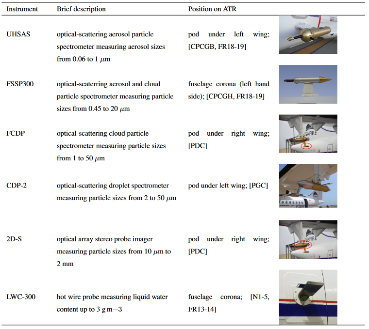
The ATR instrumentation used for EUREC4A (Fig. 7) was composed of an ensemble of in situ probes and sensors to measure the dynamical, thermodynamical and microphysical properties of the atmosphere near the aircraft; passive radiometers to measure broadband radiative fluxes and spectrally resolved infrared radiances; a laser spectrometer to measure the isotopic composition of water vapor in situ; and a lidar and two Doppler cloud radars to characterize the macrophysical properties of clouds and the presence of precipitation and aerosols away from the aircraft. All instruments are used in the EUREC4A datasets presented in this paper except the Gerber, Nevzorov, forward-scattering spectrometer probe (FSSP300) and fast cloud droplet probe (FCDP).
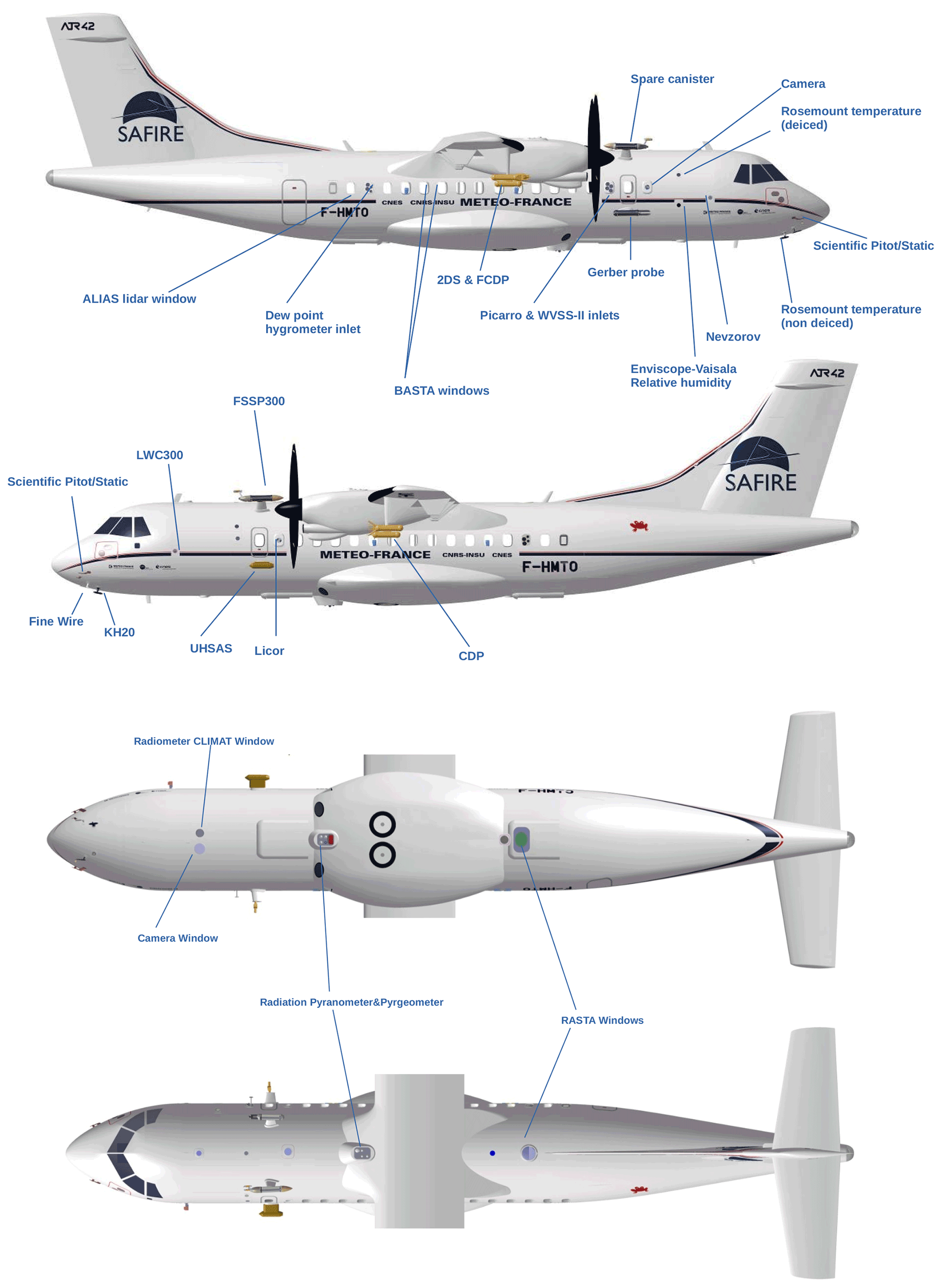
Figure 7Location on the ATR of the main instruments discussed in this paper. The panels show the aircraft from different viewpoints: right, left, bottom and top, respectively. The exact positions of each instrument are given in Tables 5 to 9. Note that the Gerber, Nevzorov, FSSP300 and FCDP probes are not used in the EUREC4A datasets presented in this paper.
The quality control, the calibration and the processing of the datasets derived from the core instrumentation of the ATR (referred to as SAFIRE-CORE, SAFIRE-RADIATION, SAFIRE-CLIMAT and SAFIRE-CAMERA), from the microphysical probes (UHSAS, ultra-high-sensitivity aerosol spectrometer, and PMA, Microphysics Airborne Platform), from the Doppler cloud radars (BASTA, Bistatic Radar System for Atmospheric Studies, and RASTA, RAdar SysTem Airborne) and from the combined radar–lidar dataset (BASTALIAS) are presented below. The processing of the lidar dataset (ALiAS, Airborne Lidar for Atmospheric Studies), the turbulence dataset (SAFIRE-TURB) and the isotopic dataset (Picarro) is fully described in separate papers (respectively Chazette et al., 2020; Brilouet et al., 2021; Bailey et al., 2022); only the main aspects of these datasets are summarized below.
3.1 Aircraft navigation, attitude and meteorological data (SAFIRE-CORE)
3.1.1 Inertial navigation system
The ATR inertial navigation system, also named AIRINS, is an iXblue inertial navigation system using a fiber-optic gyroscope. By construction, an inertial unit is drifting, and the position needs to be reset by a global positioning system (GPS) position to provide accurate parameters. It is done by using a Trimble BX992 GPS. The AIRINS-GPS positioning system then provides groundspeed, acceleration, attitudes angles and speed platform components in an Earth-based coordinate system.
During EUREC4A, three problems occurred that impacted the measurements and the data processing. (1) A failure in the internet output of the AIRINS-GPS system prevented us from recording the data at 100 Hz as usual; the data were recorded instead at 50 Hz on a serial output, and then they were synchronized and averaged at 25 and at 1 Hz. (2) During RF03, the GPS was rejected by AIRINS, which resulted in an incorrect position (true heading and attitude) and thus unreliable horizontal wind measurements for this flight; a corrected position (derived from the GPS only) was used in the V2 version of the SAFIRE-CORE dataset as well as in the RF03 files of other ATR datasets. (3) For RF20, the inertial and GPS data are available at 1 Hz only.
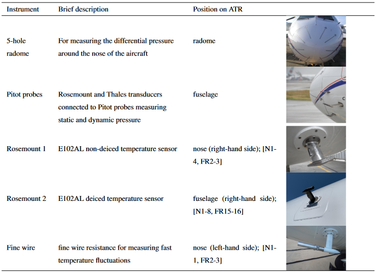
Table 5Core instrumentation of the ATR for pressure and temperature measurements. See Appendix D for the correspondence between the position H, N or FR and the ATR configuration (H refers to an aircraft window, N to the nose of the aircraft and FR to a particular position along the fuselage).
3.1.2 Pressure, anemoclinometric and wind measurements
The ATR is equipped with a five-hole radome that measures the distribution of pressure around the nose of the aircraft (Table 5): the difference in pressure measured between two holes in the vertical or horizontal planes informs about the attack angle and sideslip angle, respectively (Lenschow, 1986). The static and dynamic pressures are measured by Rosemount or Thales transducers connected to Pitot tubes on both sides of the radome. The static pressure, which corresponds to the pressure corrected from the airflow disturbance produced by the aircraft, is determined using a pre-established calibration based on specific flights and maneuvers. The dynamical pressure is obtained by subtracting the static pressure from the total pressure measured at the central radome hole. The true air speed (TAS), which is the speed of the aircraft relative to the air mass through which it is flying, is calculated from the dynamical and static pressures.
The wind is then inferred from the difference between the speed of the aircraft relative to the Earth and the true air speed (Lenschow, 1986). The high-rate wind measurements of the ATR have been very robust since its first field campaign in 2006 (Saïd et al., 2010). Unfortunately, because of a hose leak between a hole of the radome and a pressure transducer inside the radome, the measurement of the vertical wind is not reliable from RF02 to RF08. The horizontal wind measurements were not significantly affected by this problem.
3.1.3 Air temperature
During EUREC4A, the air temperature was measured by two Rosemount sensors E102AL (Table 5). The first one is located on the nose of the aircraft, inside a non-deiced housing, and the second one is located on the fuselage inside a deiced housing (Fig. 7). The static temperature, which is the temperature corrected for aircraft speed and recovery factor of the housing, is calculated as
where Tt is the measured total temperature (∘C), ΔP the dynamic pressure (hPa), Ps the static pressure (hPa) and rf the recovery factor (rf=0.98)
From RF09 to RF20, fast (turbulent) temperature fluctuations were also measured at 200 Hz (and averaged at 25 Hz) with a fine-wire temperature sensor. The fine wire is a 5 µm platinum wire soldered on a support and mounted inside a SFIM T4113 housing. Despite its fragility (a fine wire can easily break during takeoff or landing when the aircraft encounters particles or insects), it remained intact during the whole campaign. Despite its housing, the response time of the Rosemount sensor can sometimes be affected by the presence of cloud droplets (Lawson and Cooper, 1990). The fine wire can also be affected by this problem, but it recovers much more quickly, emphasizing the complementarity of the two sensors (Brilouet et al., 2021). The total temperature from the fine wire is derived by fitting and calibrating its raw measurements against the total temperature measured by the non-deiced Rosemount sensor. The resistance of the fine wire being subject to oxidation, this calibration is performed for each individual flight. The static temperature is estimated using the same method as for the Rosemount sensor, using (for the lack of a better estimate) the same recovery factor.
The Rosemount temperature data are processed at 1 and at 25 Hz, and the fine-wire temperature data are processed at 25 Hz. From RF09 to RF20, the turbulence dataset (SAFIRE-TURB) uses the fine-wire data as the best estimate for fast fluctuations and the Rosemount data as a spare (Brilouet et al., 2021).

3.1.4 Humidity
No fewer than five instruments measured humidity in situ on board the ATR (Table 6), in addition to the cavity ring-down spectrometer (CRDS) presented in another section of this paper (Sect. 3.6). Each instrument is based on a particular measurement principle or technology and therefore exhibits specific strengths and limitations in terms of stability, response rate, sensitivity to the presence of condensation or measuring range. The comparison and fine analysis of the different measurements makes it possible to calibrate and correct or bypass the shortcomings of each measurement so as to produce high-quality humidity datasets. The main features associated with these instruments and the processing of their measurements are outlined below.
A chilled mirror dew point hygrometer (Buckresearch 1011C) measured the atmospheric dew and frost points. This measurement, made by cooling a reflective condensation surface until an optical system detects the presence of condensation, is traditionally considered as a reference measurement for humidity. However, this type of hygrometer can have limitations when the aircraft undergoes large changes in altitude, passes through a cloud or samples environments with high humidity contrasts. This sensor also has a slow response time and shows limitations in very dry conditions such as those encountered above the trade inversion.
A Humicap 180C enviscope–Vaisala capacitive sensor was placed inside a non-deiced Rosemount E102 housing. This sensor is made of a hygroscopic dielectric material whose capacitance is dependent on humidity. After correcting for the effects of aircraft speed, it measures relative humidity directly with a short response time. However, the sensor is sensitive to the presence of cloud droplets, and it can report relative humidities above 100 %. Its measurements are thus considered only in unsaturated environments, and under these conditions they help assess the robustness or even calibrate the measurements of other sensors mentioned above.
Unlike previous sensors, the Water Vapor Sensing System version two (WVSS-II; Fleming and May, 2004) designed by SpectraSensors for use on commercial aircraft can measure humidity with a good reliability and regularity, without being affected by the presence of cloud droplets or very dry air (Smit et al., 2014; Vance et al., 2015). This is due to its particular technology, based on tunable diode laser absorption spectroscopy in the near-infrared (1.37 µm), and to the fact that its sampler has been designed to minimize the biases associated with the presence of cloud droplets or aerosols. Therefore, for this campaign it is considered as a reference for slow humidity measurements, and it is used to adjust or calibrate humidity measurements from other sensors. The WVSS-II measures the mixing ratio of water vapor relative to dry air in parts per million volume (ppmv). The volumic concentration is converted to a mass concentration to provide absolute humidity measurements in grams per cubic meter.
Finally, two additional instruments were used to measure rapid fluctuations in humidity: a Licor LI-7500A and a Campbell Scientific krypton hygrometer (KH20).
The Licor LI-7500A is a near-infrared gas analyzer originally designed to measure eddy-covariance fluxes on ground towers, which has been adapted by SAFIRE to perform airborne measurements (Rozen and Muskardin, 2007) in replacement of the historical reference Lyman-alpha instrument (Buck, 1985; Friehe et al., 1986). Lampert et al. (2018) present a comparison of the two sensors. Its strength lies in its short time response, but its main limitation is its high sensitivity to the presence of liquid water (its performance can be affected even a few seconds after leaving a cloud). Periods when the humidity measurement is affected by condensation (typically inside clouds) are detected on the basis of the strength of CO2 measurements made by the same sensor. The Licor performance can also be affected by the presence of sea salt, particularly when the aircraft is flying low near the sea surface. To minimize this problem, the lowest legs were performed at the end of the flight, and the Licor window was cleaned before each subsequent flight. The Licor humidity measurements (g m−3) are calibrated against the WVSS-II absolute humidity measurements of RF13, and the same calibration coefficients are used in all flights (note however that the calibration of humidity in the SAFIRE-TURB dataset is performed leg by leg as described by Brilouet et al., 2021). As the Licor clock is initialized manually, it is sometimes delayed by a few seconds. This delay is subsequently corrected during post-processing. The corrected and synchronized time parameter of the Licor instrument is also used to correct a delay of 3 s of the WVSS-II sensor induced by the interface of the instrument. Note that Licor data were not recorded during the flights RF05 and RF06.
The KH20 uses the absorption of the UV light emitted at 123.58 and 116.49 nm by a krypton lamp to estimate the water vapor density (Campbell et al., 1985; Foken and Falke, 2012). This instrument has also been originally designed for eddy-covariance measurements on ground towers, but Kotani and Sugita (2004) had reported its use on an aircraft. The instrument has been heavily modified by SAFIRE to be operated on the ATR (Charoy, 2015): the housing of an older humidity sensor (a Lyman-alpha hygrometer) was used to install the source lamp and detector, and the electronic box was installed inside the cabin. This sensor was less sensitive to the presence of cloud droplets than the Licor, but it was more affected by sea salt. Therefore, as the Licor it was cleaned before each subsequent flight. The KH20 measures rapid fluctuations in humidity but not absolute humidity. Absolute values (g m−3) are obtained by calibration against the slow (1 Hz) humidity measurements of the WVSS-II (Brilouet et al., 2021).
Based on the processing of these different measurements, two humidity datasets have been produced: one at 1 Hz, included in the SAFIRE-CORE dataset, and another at 25 Hz, which is included in the SAFIRE-TURB dataset. Note that in the SAFIRE-TURB dataset, the calibration of the humidity measurements is performed on a leg-by-leg basis, for both the Licor 7500A and the KH20 sensors.
Table 7Core instrumentation of the ATR for radiative measurements. See Appendix D for the correspondence between the position on the aircraft and the ATR configuration.
3.2 Radiative measurements
3.2.1 Broadband radiative fluxes (SAFIRE-RADIATION)
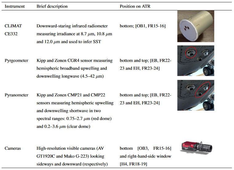
Kipp & Zonen sensors mounted at the top and at the bottom of the ATR measured upwelling and downwelling broadband radiative fluxes, respectively (Table 7): CGR4 pyrgeometers measured hemispheric longwave fluxes in the 4.5–42 µm spectral range, CMP21 pyranometers measured hemispheric shortwave radiation in the 0.75–2.7 µm spectral range (red dome), and CMP22 pyranometers measured hemispheric shortwave radiation in the 0.2–3.6 µm spectral range (clear dome).
Measuring upwelling and downwelling radiative fluxes requires the aircraft to be in a plane and stable position. For this reason, the SAFIRE-RADIATION dataset includes two sets of variables for each radiative flux: raw fluxes and fluxes corrected for the attitude of the aircraft. In the time series of corrected fluxes, whenever the roll or pitch of the aircraft was greater than ±5∘ the radiative measurements were considered to be “undefined”, and otherwise the downwelling shortwave measurements were corrected for the attitude of the aircraft. This correction requires knowledge of the offset of the sensor installation, which corresponds to the bias associated with the potential tilt of the mechanical installation of the sensors relative to their support. This offset must be estimated every time the sensor has been remounted on the aircraft (as done at the arrival of the ATR in Barbados; Sect. 2.1). It was determined through specific maneuvers performed during the test flight RF02.
All pyrgeometers and pyranometers worked properly during the campaign except one: the CMP21 pyranometer (red dome) at the top of the aircraft. Because of this malfunctioning, the downwelling 0.75–2.7 µm irradiance measurements were either absent or invalidated during the campaign. However all other upward and downward longwave and shortwave fluxes, including the downwelling shortwave measurements over the 0.2–3.6 µm spectral range, are available and distributed in the SAFIRE-RADIATION dataset at 1 Hz.
3.2.2 Infrared brightness temperatures (SAFIRE-CLIMAT)
In addition to broadband radiometers, the ATR carried a nadir-viewing multispectral radiometer, the CLIMAT CE332 instrument, developed by the Laboratoire d'Optique Atmosphérique (LOA) in collaboration with CIMEL (Brogniez et al., 2003). This radiometer measures infrared radiances and brightness temperatures at three wavelengths: 8.7, 10.6 and 12 µm (Table 7). It is done by comparing the radiances measured on the observed target with that measured by looking at a reference cavity maintained at a given temperature. During the post-processing, the measurements performed at 6 Hz are synchronized and averaged at 1 Hz. They are included in the SAFIRE-CLIMAT dataset. It is planned to estimate the sea surface temperature from these measurements.
3.2.3 Visible images (SAFIRE-CAMERA)
To visualize the context of the data acquired by in situ measurements or remote sensing, two high-resolution cameras were mounted on the aircraft. One camera, an AV GT 1920C model with a resolution of 1936 × 1456 pixels and a wide angle (focal length of 4.8 mm), took high-frequency images (10 frames per second) through the ATR window on the side of the horizontally staring lidar and radar instruments. The other camera, a Mako G-223 model with a resolution of 2048 × 1088 pixels and a focal length of 16 mm, looked down towards the sea surface at a moderate frequency (1 frame per second). The images taken through the aircraft windows often appear dark because the choice of exposure time was made to avoid saturation due to the brightness of the clouds as much as possible, especially when the sun is behind the aircraft (Fig. 8a). The downward-looking camera can detect the presence of clouds below the aircraft and can help characterize the state of the ocean surface (Fig. 8b).
Three types of products are derived from these cameras: movies (in avi format) are produced for each camera (“window” or “ground”) and for each flight, and high-resolution images (in bmp format) are produced for the window camera for R and L patterns.
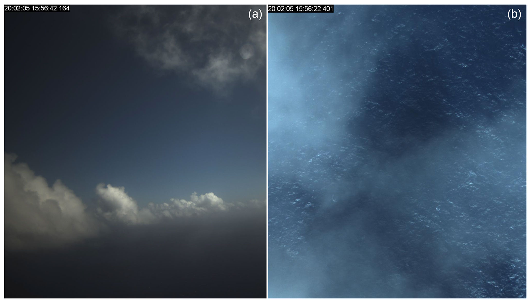
Figure 8(a) Example of a cumulus scene captured by the visible camera through the aircraft window on 5 February 2020 at 15:56 UTC. (b) Image acquired a few minutes earlier by the camera looking down towards the ocean.
3.3 In situ turbulence measurements (SAFIRE-TURB)
The five-hole nose radome and specific temperature and humidity sensors mounted on the ATR (Rosemount and fine-wire thermometers, Licor and KH20 hygrometers; see Tables 5 and 6 and Sect. 3.1) measured rapid fluctuations in the three wind components, temperature and humidity. Based on these high-frequency (25 Hz) measurements, the SAFIRE-TURB turbulence dataset was produced to characterize the turbulent characteristics of the atmosphere through a number of diagnostics. The data processing strategies, the calibration methodologies, the procedures of quality control applied to the 25 Hz temperature and moisture measurements, and the methods used to estimate the turbulent diagnostics are explained in detail in Brilouet et al. (2021).
The dataset includes two kinds of products: “turbulent fluctuations” and “turbulent moments”. The “turbulent fluctuations” include time series of high-frequency fluctuations in the dynamical and thermodynamical variables over straight and stabilized segments of T-shortlegs, T-longlegs or T-longestlegs (Table 2). For each segment, the fluctuation time series are either detrended (“DET”) or high-pass-filtered (“FIL”) with a cutoff frequency of 0.018 Hz (about 5 km wavelength). The comparison of the “DET” and “FIL” calculations informs about the homogeneity of the sample and about random and systematic sampling errors.
The “turbulent moments” include means, variances and covariances of dynamical and thermodynamical variables, turbulent kinetic energy and dissipation rate, third-order moments and skewnesses of wind components, potential temperature, and water vapor mixing ratio. They also include characteristic length scales such as the integral length scale or the wavelength of the vertical velocity density energy spectrum peak, error estimates on the turbulent moments, and quality flags on the wind, temperature and humidity measurements. These diagnostics are produced for each type of segment (T-shortlegs, T-longlegs and T-longestlegs).
This dataset is produced for two levels of data processing. In the Level 2 dataset, the turbulent moments and fluctuations are calculated for each humidity sensor and each temperature sensor, and a quality flag is associated with each sensor. In the Level 3 dataset, a “best estimate” of the turbulent moments and fluctuations is provided, together with a quality flag; for each segment, the best estimate corresponds to the moments and fluctuations computed from the sensor that has the best quality flag over this segment. The dataset is distributed in NetCDF files whose nomenclature is summarized in Table 3 of Brilouet et al. (2021).
Table 8Microphysical probes mounted on the ATR for EUREC4A. See Appendix D for the correspondence between the position on the aircraft and the ATR configuration.
3.4 In situ aerosol and cloud measurements
The ATR payload included a suite of six instruments to measure in situ aerosol and cloud properties (Table 8). The ultra-high-sensitivity aerosol spectrometer (UHSAS), the FSSP300 and the LWC-300 were operated by SAFIRE. The cloud droplet probe (CDP-2), the fast cloud droplet probe (FCDP) and the 2D stereo probe (2D-S) are part of the Microphysics Airborne Platform (PMA), a French national facility operated by LaMP (Laboratoire de Météorologie Physique). Before takeoff, all the data acquisition systems were synchronized to the aircraft central time database (GPS). All instruments but the UHSAS are open-path instruments with fast electronics, and therefore their response time is negligible. The potential plumbing delay of the UHSAS (estimated to be of the order of a second) is not taken into account for now.
3.4.1 Aerosols (UHSAS)
A UHSAS-A probe (airborne version, serial no: 1303-007) was mounted on the lower left-hand pod on the fuselage section (Fig. 7). This probe is an optical-scattering aerosol particle spectrometer developed and commercialized by Droplet Measurement Technologies (DMT) that counts and sizes particles in the 0.06 to 1 µm range. The sizes are then sorted into 99 linearly spaced size bins of fixed width (9.7 nm).
The operating principle is as follows: the external air drawn at a controlled flow rate (about 50 sccm) enters the instrument optical detector, where it is aerodynamically focused and brought through a laser beam (Nd3+:YLiF4 laser operating at 1053 nm). The laser light scattered by each aerosol particle is collected by two pairs of Mangin collection optics, and the scattered intensity is measured with a dual Avalanche photodiode low-gain PIN photodiode detection system. The size of each particle is derived from the scattered intensity by using Rayleigh (40–300 nm) or Mie (300–1000 nm) scattering models implemented in the instrument (they are not corrected for variations in particle refractive index or non-sphericity). The UHSAS-A used in EUREC4A was last maintained and calibrated by DMT in December 2018 (using National Institute of Standards and Technology traceable polystyrene spheres of nominal diameter 100 nm), and a calibration check (using polystyrene beads of various sizes, e.g., Thermo Fisher Scientific 3150A) was performed at SAFIRE prior to the campaign in May 2019.
According to the manufacturer, UHSAS operation is limited to a non-condensing environment. Ladino et al. (2017) reported that UHSAS measurements are subject to water contamination when performed in a cloudy area, which is also visible in our data. Therefore, UHSAS measurements made in cloudy areas (determined by liquid water content >1 mg m−3 using CDP and 2D-S data, as in the case of Ladino et al., 2017) are rejected. Moreover, the UHSAS has a maximum count rate of 3000 s−1, and Cai et al. (2008) have shown that the detection efficiency decreases when the particle concentration exceeds 3000 cm−3 due to a coincidence effect. Therefore, points where the total count exceeds 3000 s−1 are removed from the data. According to Cai et al. (2008), particle concentrations in the small size range come with a caveat that the detection efficiency of a UHSAS (lab version) tends to decrease for particles smaller than 100 nm. Finally, inspection of the housekeeping data revealed erratic variations in the sample flow rate between 32 and 50 sccm, caused by a loose electrical connection at a mass flow controller. Periods of large sample flow variation are manually identified and discarded. The aerosol concentration is calculated from the probe counts per second and the sample flow rate converted from mass (sccm) to volumetric flow rate (cm−3) using temperature and pressure measurements from the aircraft core instruments (Sect. 3.1.2 and 3.1.3).
The total concentration of aerosol particles and the particle size distribution measured by UHSAS during the different ATR flights are shown in Fig. 9. The concentrations in the subcloud layer and out of the cloud at the cloud base level are generally similar, although a few flights (RF06, RF11, RF15 and RF17) show a slightly reduced concentration at the cloud base level. In every case, the concentration is highly variable (Table 4 and Sect. 2.5), with two main regimes: average aerosol concentrations are about 100 cm−3 in half of the flights and about 300–400 cm−3 in the other half. The particle size distribution also varies among flights, with the highest variability occurring in the frequency of large particles (diameters larger than 300 nm).
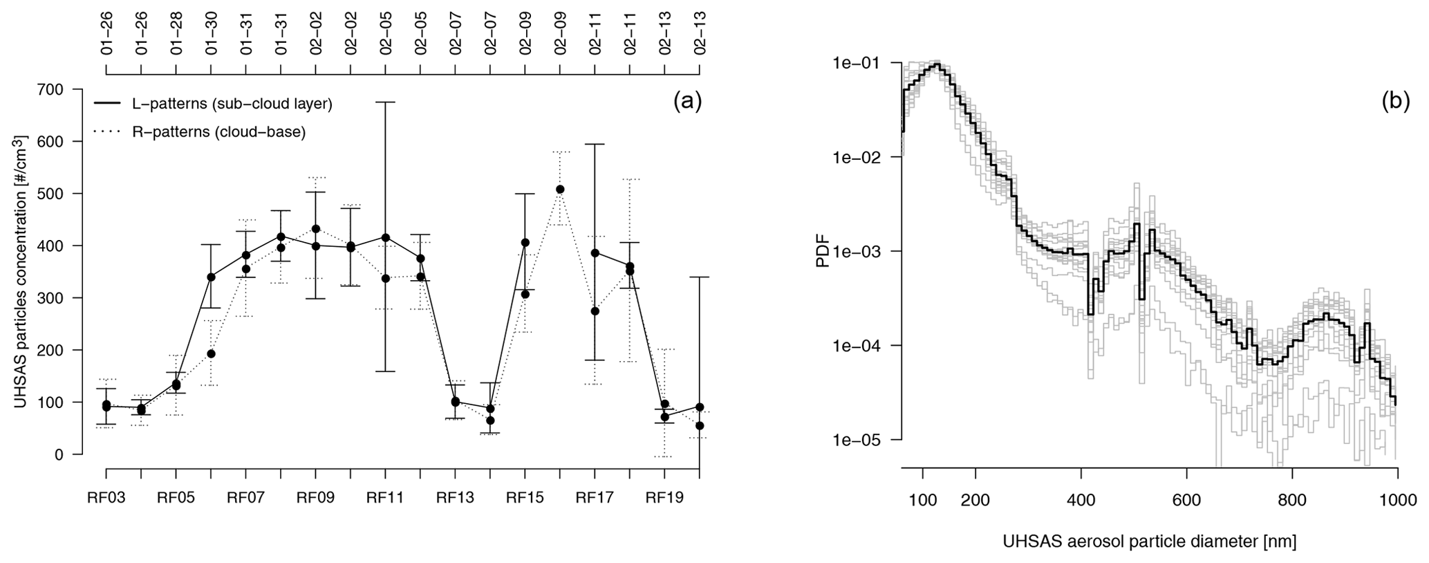
Figure 9(a) Evolution of the total concentration of aerosol particles (cm−3) within the subcloud layer and at the cloud base level derived from UHSAS data (vertical bars represent the standard deviation across the different R patterns or L patterns during each flight). Note that the time axis is not linear, and markers are only related by a line to ease readability. (b) Probability distribution function of the aerosol particle size derived from UHSAS data over the R patterns flown at cloud base; the mean of each ATR flight is shown in gray, and the mean over all flights is shown in black.
3.4.2 Cloud microphysics
Cloud microphysical measurements were made with two instruments: the CDP-2 (Lance et al., 2010), which counts and sizes cloud droplets in the 2–50 µm size range, and the 2D-S (Lawson et al., 2006), which images cloud, drizzle and raindrops in the 10–1280 µm nominal size range (Table 8). Both instruments were mounted under the wings of the ATR, one on the right side and the other on the left side (Fig. 7). Throughout the campaign, the optics of the 2D-S and CDP-2 (and FCDP) probes were cleaned after each flight to remove traces of dust and salt. At low altitudes, where the air is warm, the temperature of the CDP-2 and 2D-S lasers increased rapidly, and therefore the instruments were often switched off by the operator to avoid damaging the probe. As a result, few CDP-2 and 2D-S measurements are reported along the subcloud-layer legs.
CDP-2: cloud droplets
The CDP-2 (serial no. 1711-111, equipped with anti-shatter tips) is a cloud particle spectrometer that counts and sizes cloud droplets in the 2–50 µm range and sorts them into 30 size categories with a resolution of 1–2 µm. The 1 Hz raw data (histograms of counts per second) are processed using DMT's built-in counting and sizing algorithms based on the Mie scattering model, assuming that droplets are spherical with a refractive index of 1.33, and converted to concentrations with the probe sample volume. The sample volume is calculated using the true air speed of the aircraft from SAFIRE-CORE data and the calibrated sample area (0.292 m2) determined prior to the campaign by mapping the probe's response to calibrated water microdroplets injected across the laser beam with an apparatus similar to Lance et al. (2010). At 100 m s−1, which was the typical ATR airspeed during the scientific flights, the sample volume was about 30 cm3 s−1. The calibration of the CDP-2 with respect to particle size was regularly monitored during the campaign by means of calibrated glass bead injection tests.
Measurements in the subcloud layer reveal that the CDP-2 can detect non-cloud droplet particles such as large and ultra-large aerosols. Although these particles may not satisfy the underlying assumption of the CDP-2 sizing algorithms, it was decided not to filter out these measurements in the CDP-2 files so that further investigations of large aerosols may be conducted, at least qualitatively. However, the response of the CDP-2 to such aerosol particles being unknown, the data taken in non-cloudy areas are subject to unquantified errors.
2D-S: cloud droplets, drizzle and raindrops
The 2D-S (serial no: 006) is an optical array probe imaging cloud, drizzle and rain particles in the range 10–1280 µm (the stereo capability of the probe is not used here): an array of 128 photodiodes is illuminated by a laser sheet; when a hydrometeor crosses the sample area (about 0.128 cm × 6.3 cm, located between a pair of emitting and receiving arms), it shades some of the photodiodes. The binary state (occulted, non-occulted) of the photodiodes is recorded at high frequency (up to 17 MHz for this probe), producing time-discretized black-and-white slices of the particle's silhouette, which are subsequently concatenated to reconstruct a projected 2D black-and-white image of the hydrometeor with a resolution of 10 µm. The calibration of the 2D-S probe was tested before the campaign with opaque calibrated features printed on glass spinning disks.
The raw data (from either the vertical or horizontal channel, whichever worked best during the flight) are processed using the LaMP in-house processing routines, which stem from the early release of the SPEC 2DSView software and are continually updated to integrate state-of-the-art corrections.
The calculation of the sample volume takes into account the decrease in depth of field with particle size and follows the manufacturer's formula given in Lawson et al. (2006) and the overload periods of the probe. Artifacts due to noisy or dead pixels are identified and removed using the pixel analysis described in Lawson (2011). This probe is equipped with anti-shattering arm tips (K-tip; Korolev et al., 2013) designed to prevent ice and droplet fragments from falling into the probe sample volume and contaminating the measurement at the lower end of the size spectra (note that no ice was sampled along the ATR flights of EUREC4A). In addition to the K-tip, a splash and shatter detection and removal algorithm based on arrival time analysis is applied (e.g., Field et al., 2006; Korolev and Field, 2015). The size of particles seen out of focus is corrected using the Korolev (2007) diffraction correction. Despite these efforts to clean artifacts, the concentration in the first few bins remains questionable for reasons described in Thornberry et al. (2017) and Bansemer (2018) (the contribution of remnant noisy events is amplified in the concentration calculation due to the small sample volume). The size of truncated particles (partial images) is corrected according to Korolev and Sussman (2000), and the nominal size range (10–1280 µm) is extended to 2.56 mm in post-processing.
Once most of the artifacts have been corrected, a series of geometrical descriptors, e.g., size (defined here as the diameter of a circle having an area equal to the projected area of the particle, often referred to as surface-equivalent diameter in the literature, Deq), area or perimeter, are retrieved from each individual 2D image. Statistical properties are then calculated at 1 Hz, such as the particle size distribution (PSD) or the total concentration (NT; calculated as the sum of bin concentrations). The mass size distribution (MSD) is computed from the PSD assuming that the particles are spherical with a liquid water density of 1 g cm−3.
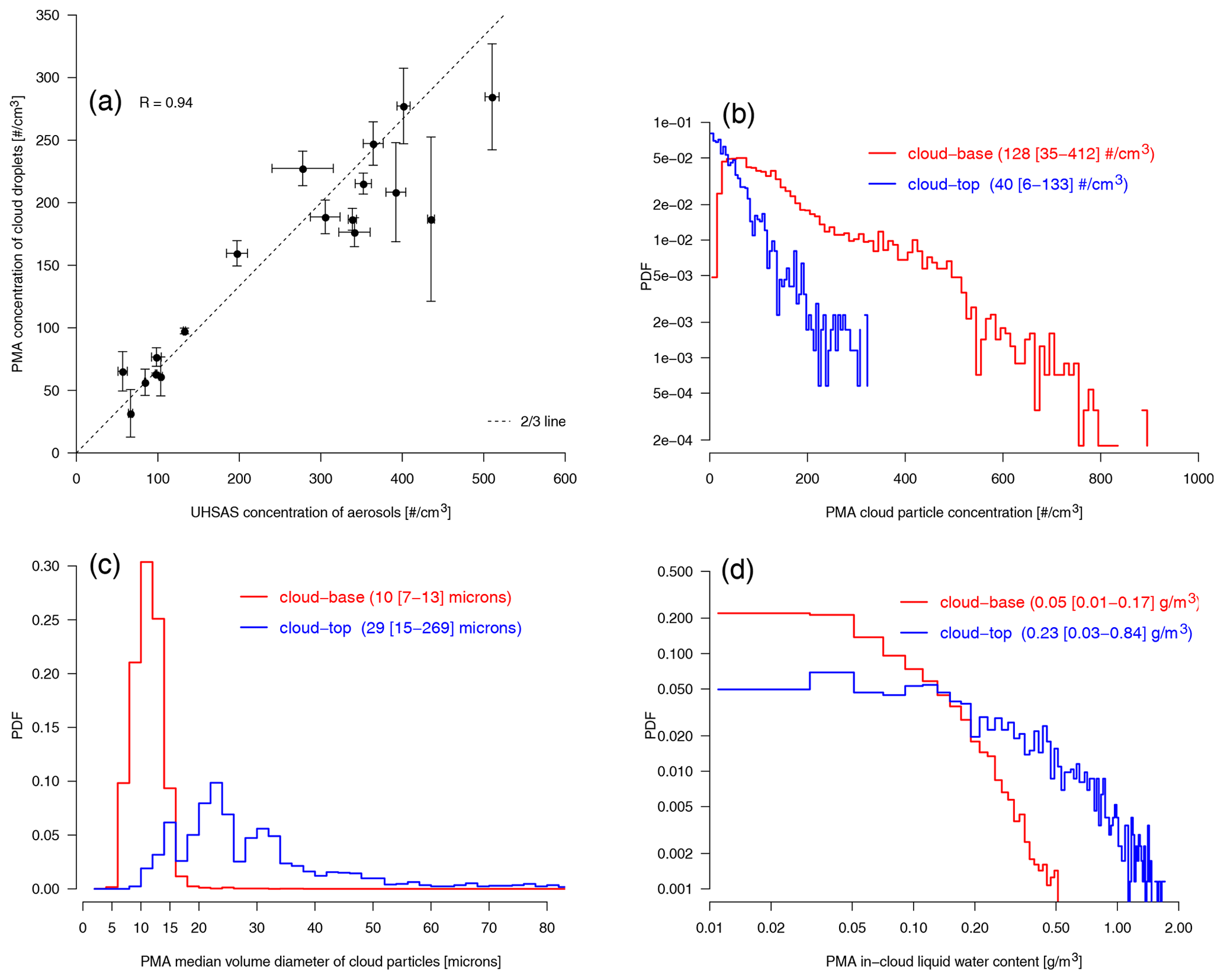
Figure 10(a) Relationship between the concentration of aerosols (from the UHSAS dataset) and the concentration of cloud droplets (from the PMA dataset, excluding drizzle and rain particles) calculated for the R patterns flown at cloud base during the whole EUREC4A campaign. The mean of each ATR flight is reported together with the standard deviation among the different R patterns of the flight. Other panels (b, c, d) show the probability distribution function (calculated over all the R patterns flown at cloud base or at cloud top) of (b) the total concentration of cloud particles, (c) the median volume diameter (MVD) of cloud particles and (d) the in-cloud liquid water content (LWC) derived from the composite PMA dataset. The median of each quantity is reported, together with the 10th and 90th percentiles of each distribution (in brackets). (b–d) Histograms are calculated for in-cloud conditions (where cloud particles can coexist with drizzle or rain particles).
PMA composites
As the cloud drop size distribution is broad, a combined PMA dataset is produced that merges the CDP-2 and 2D-S data into a single composite spectrum that ranges from 2 µm to 2.55 mm, at the native size resolution of the CDP-2 up to 43 µm, the 10 µm size resolution of the 2D-S up to 1 mm and a coarser resolution of 100 µm from 1.05 up to 2.55 mm. To do so, the 2D-S size distributions are interpolated to match the CDP-2 bin resolution on the 10 to 50 µm overlap region. When data from both probes are available, we use CDP-2 data up to 31 (±1) µm; between 33 and 43 (±1) µm, we use the average of CDP-2 and 2D-S concentrations; and beyond 50 (±5) µm, we use 2D-S data. When CDP-2 data are not available (data are set to NaN (not a number, i.e. undefined value) values whenever a probe does not operate), the first two bins of the 2D-S are omitted such that the composite spectra start at 30 (±10) µm. Note that a ±1 s offset was added to the 2D-S data whenever it improved the correlation between the LWC retrieved from the CDP and 2D-S data in the 25–45 µm overlap region.
As the CDP and 2D-S were mounted on two different wings about 10–15 m apart (Table 8), it could happen that only one of the two wings crossed a cloud, thus generating some inconsistency between the measurements of the two probes. Therefore, the composite product comes with a variable (compo_index) that describes the composite and qualifies the overlap between the two sondes (1: CDP data only; 2: 2D-S data only; 3: CDP and 2D-S in good agreement; and 4: CDP and 2D-S in poor agreement). In the future, inconsistencies could be limited by producing another composite that would use the 2–50 µm measurements from the FCDP probe (rather than the CDP) as this probe was mounted just below the 2D-S.
From the composite size distributions we calculate microphysical quantities such as the total concentration of particles (NT); liquid water content (LWC; third moment of the distribution assuming a density of 1 g cm−3); median volume diameter (MVD; defined as the median of the cumulative mass size distribution); and a series of masks that indicate the presence of cloud, drizzle or rain drops.
We define a cloud mask and a drizzle mask based on the LWC and the particle size (diameter D): a cloud particle is identified when the LWC of droplets smaller than D0 exceeds LWC0, where LWC0 and D0 are specified thresholds of LWC and D, respectively. There is no simple definition of cloud situations, and therefore the values of these thresholds remain uncertain. Here, we use LWC0 =0.010 g m−3 (which is consistent with other observational and modeling studies of trade-wind clouds such as Heymsfield and McFarquhar, 2001, or van Zanten et al., 2011) and D0 =100 µm (which is consistent with the AMS glossary definition of cloud drops as water particles between 1 and 100 µm in diameter). We assume that drizzle occurs (drizzle mask is set to 1) when µm, and rain occurs when D≥500 µm.
The cloud LWC was inferred from the size distribution of cloud particles measured by the CDP-2 and 2D-S probes. It was also measured independently by a hot-wire probe (DMT LWC-300) that was part of the core instrumentation of the ATR (Table 8; note that the LWC-300 sensor broke during RF14 and was immediately replaced by a new one). The hot-wire estimates the LWC by measuring the heat released by the vaporization of water droplets on a heated cylinder exposed to the airstream. This calculation is made with the Particle Analysis and Display System (PADS) software, using the aircraft airspeed, pressure and deiced temperature measured by the ATR and the formulas given in the DMT PADS Manual Hot Wire Module 3.5.0 DOC-0290 Rev A. However, the collection efficiency of the sensor is limited for small droplets (< 10 µm), and the evaporation of large drops (>50 µm) can be incomplete, which can underestimate the LWC measurement in drizzle and rain conditions when such large drops are present (DMT LWC-300 LWC operator's manual DOC-0361 Rev C). The LWC estimate derived from the CDP-2 and 2D-S probes (distributed in the PMA composite dataset) is thus considered to be more precise than that derived from the LWC-300 (distributed in the SAFIRE-CORE dataset).
Cloud droplet number concentrations at cloud base and their relationships with aerosol number concentrations (derived from UHSAS) are shown in Fig. 10a. Cloud droplet number concentrations tend to be about of the aerosol concentrations, with a strong case-to-case co-variability (correlation of 0.94). At larger aerosol concentrations, the cloud droplet concentrations are disproportionally less in cases with larger aerosol concentrations. This could be indicative of a lower maximum of cloud base supersaturations in an aerosol-rich environment or a less cloud-active aerosol in conditions when the concentrations are high. However, such a sublinear relationship between cloud condensation nuclei (CCN) and cloud drop concentration is not uncommon, and different interpretations have been proposed for this feature, including a measurement artifact known as “coincidence” (Lance, 2012). Since the CDP-2 probe is prone to coincidence errors at concentrations as low as 200 cm−3 (Lance et al., 2010), in this case an instrumental artifact cannot be ruled out without further investigation.
The distribution along all the R patterns of the droplet number concentration, MVD and LWC values of the clouds derived from the PMA composite dataset is shown in Fig. 10b–d. Cloud particle concentrations are very variable, but, on average, they tend to be much larger at cloud base (median of 128 cm−3) than in the stratiform layers of trade cumuli detraining near the inversion level (median of 46 cm−3); on the other hand, cloud particle sizes and cloud liquid water contents tend to be much smaller at cloud base (about 10 µm and 50 mg m−3, respectively) than at cloud top (about 24 µm and 200 mg m−3 near the inversion level). The range of MVD values measured near cloud base and cloud top during EUREC4A are similar to those measured in trade cumuli over the Indian Ocean (Heymsfield and McFarquhar, 2001) or in cumulus clouds over the sea around the UK (Raga and Jonas, 1993).
3.4.3 Datasets
An aerosol dataset was produced on the basis of UHSAS measurements. It is distributed as an ensemble of NetCDF files (one file per flight) that include products such as the PSD and NT, all processed at a frequency of 1 Hz.
A cloud dataset was produced on the basis of CDP-2 and 2D-S measurements (future versions of the dataset might include data from the FSSP-300 and FCDP probes). It is distributed as a set of NetCDF files (one file per flight) which include products such as PSD, NT and LWC (assuming that particles are spherical with a density of 1 g cm−3), all processed at a frequency of 1 Hz.
The data are distributed for two levels of processing: the Level 2 dataset is associated with single instruments (either 2D-S or CDP-2), while the Level 3 dataset corresponds to a combined PMA dataset that merges CDP-2 and 2D-S data into a single composite spectrum that spans the range 2 µm to 2.55 mm. The composite dataset includes additional products such as a cloud mask, a drizzle mask and a rain mask (defined in Sect. 4.3) as well as the sixth moment of the particle size distribution to ease the comparison with radar reflectivities. The periods of flight when the probes are switched off are filled with NaN values. All datasets also include the time and aircraft position from the SAFIRE-CORE dataset.
The LWC measurements from the LWC-300 are included in the SAFIRE-CORE dataset at 1 Hz.
3.5 Lidar and radar remote sensing
3.5.1 Horizontal lidar measurements (ALIAS)
Table 9Lidar–radar remote sensing and stable isotopologue measurements. See Appendix D for the correspondence between the position on the aircraft and the ATR configuration.

To characterize the presence of clouds and aerosols in the lower troposphere, the ATR was equipped with a lightweight backscatter lidar named ALiAS (Airborne Lidar for Atmospheric Studies) emitting at the wavelength of 355 nm and detecting polarization (Table 9; Chazette et al., 2012, 2020). The main role of this lidar was to measure, together with the BASTA radar described next, the fractional area covered by the cloud field near the cloud base level. For this purpose, the line of sight of the lidar was oriented horizontally, looking through one of the ATR windows (UV fused silica glass) on the right side of the aircraft (Fig. 7).
The native resolution of the lidar backscatter profile along the line of sight is 0.75 m. However, to improve the signal-to-noise ratio, a low-pass filter has been applied, and the resolution was downgraded to 15 m. In addition, the backscatter profile was averaged over 50 consecutive shots during the acquisition, which corresponds to approximately one recording every 5 s (averaging time of 2.5 s and recording time of 2.5 s). The backscatter lidar observations are used to define a cloud mask in the direction perpendicular to the aircraft trajectory. In this direction, the signal was distinguishable from noise up to a distance of about 8 km in clear-sky conditions. However, this range was reduced in the presence of strong scattering, for instance from thick clouds. It means that during the R patterns, as the aircraft was flying rectangles of about 120 km (along track) × 20 km (cross track), the lidar was able to sample most of the rectangle area unless thick clouds within the rectangle extinguished the lidar signal at some distance of the aircraft.
Both aerosol and cloud products have been derived from the ALiAS observations, and the data are distributed as a set of NetCDF files (one per flight) for different levels of processing. Level 1 provides the raw profiles at native resolution recorded by the acquisition system. Level 1.5 data are geolocated, calibrated and corrected for geometric factors and molecular transmission, and time series of the apparent backscatter coefficient (ABC) and volume depolarization ratio (VDR) are produced with a resolution of 15 m along the lidar line of sight. Level 2 provides cloud and aerosol detection information and products, including a cloud mask and an aerosol extinction coefficient (AEC) along the horizontal line of sight. Level 3 provides statistics about the length of the cloud chords inferred from the lidar cloud detection. The ALiAS dataset is described in detail in Chazette et al. (2020).
Figure 11 shows the relationship between the total concentration of particles measured by the UHSAS microphysical probe (Sect. 3.4.1) and the aerosol extinction coefficient retrieved from ALiAS lidar data. Although the two instruments sample the atmosphere very differently (the lidar probes the atmosphere horizontally perpendicular to the aircraft trajectory over a range of several kilometers, while the UHSAS probes the atmosphere in situ along the aircraft trajectory), the two measurements are highly correlated (R=0.89). It shows the consistency of the two measurements and confirms the strong variability in the atmospheric load in aerosols during the campaign (Fig. 9).
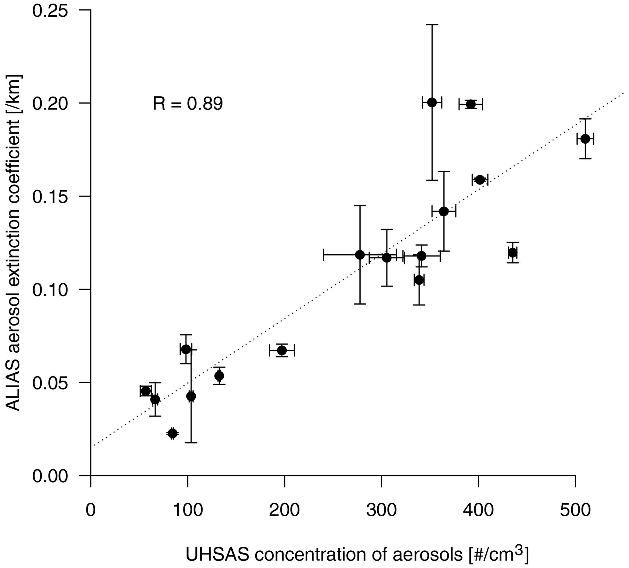
Figure 11Relationship between the total concentration of aerosols measured by UHSAS at cloud base and the aerosol extinction coefficient measured by the horizontally pointing ALiAS lidar at cloud base. Horizontal and vertical bars represent the standard deviation of measurements across the different R patterns of each flight.
3.5.2 Horizontal radar measurements (BASTA)
To characterize the cloudiness in synergy with the lidar, a horizontally staring cloud radar named BASTA (Bistatic Radar System for Atmospheric Studies) was mounted on the right-hand side of the ATR (Table 9). BASTA is a 1 W bistatic FMCW (frequency-modulated continuous-wave) 95 GHz Doppler cloud radar developed from the ground-based BASTA system (Delanoë et al., 2016). It was used in an aircraft for the first time during EUREC4A, with two antennas of 20 cm (0.95∘ beamwidth) installed in back lateral windows of the ATR (Table 9). The radar was operated in two modes, one after the other, at 12.5 and 25 m range resolutions with 0.5 and 1 s time resolutions, respectively. It led to a measurement in one mode every 1.5 s. The maximum range was 12 km with an ambiguous velocity of 9.85 m s−1 for both modes. The minimum detection range is about 80 m from the aircraft due to coupling between the two antennas.
The Level 1 of the BASTA product contains, for both modes, the calibrated and range-corrected radar reflectivity, the Doppler velocity, and a mask distinguishing the meteorological target from background noise and surface echoes. The calibration of the radar has been derived from other field campaigns and confirmed using in situ data by calculating a reflectivity from the CDP and 2D-S cloud particle data and comparing it with radar measurements in cloudy conditions. The sensitivity of the radar is estimated at around −35 dBZ at 1 km. Level 2 data are the most elaborated product, the two modes being combined to optimize the advantages of each range resolution. Within the first 250 m, the 12.5 m mode is used, while the 25 m mode covers the rest of the profile. The combined reflectivity and Doppler profiles are available every 1.5 s. The radar gates are geolocated in latitude, longitude and altitude in order to derive maps. The reflectivity is corrected for gaseous attenuation using colocated information from dropsonde temperature, humidity and pressure. A parameterization of liquid attenuation for both cloud and precipitation as a function of reflectivity was derived thanks to in situ data and applied to correct reflectivity for liquid attenuation. The corrected reflectivity is then used to distinguish cloud areas from drizzle or rain (Sect. 3.5.3). The radar Doppler velocity is corrected for aircraft motion and folding using gate-to-gate correction. All files are available in a self-documented NetCDF file.
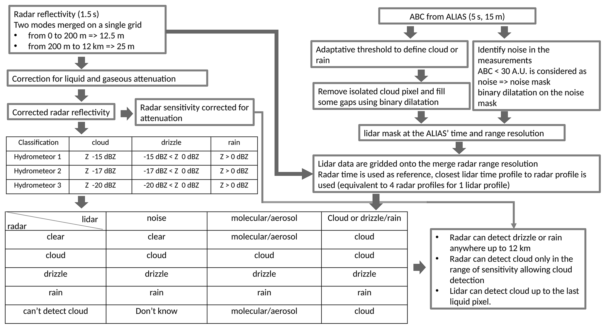
Figure 12Cloud detection algorithm applied to BASTA and ALiAS data to detect hydrometeors (clouds, drizzle and rain).
3.5.3 Combined lidar–radar measurements (BASTALIAS)
Based on ALiAS and BASTA data, a combined dataset was developed that takes advantage of the lidar–radar synergy and complementarity to improve the detection of clouds, drizzle and rain (Fig. 12).
For this purpose, the two modes of the BASTA radar products are merged on a single horizontal grid (resolution of 12.5 m within the first 200 m from the aircraft and 25 m beyond this distance) and a single time resolution (1.5 s). Then the reflectivity is corrected for liquid and gas attenuation, and the radar sensitivity is defined as a function of the distance from the aircraft. A first classification of hydrometeors is then made on the basis of radar observations. As the reflectivity associated with the presence of a remote hydrometeor depends on the drop diameter, reflectivity thresholds can be used to distinguish cloud droplets from drizzle or rain. The definition of these thresholds differs across ground-based radar studies; the threshold distinguishing clouds from drizzle (Zd) is often set at −20 dBZ (e.g., Kato et al., 2001), but it can also be set at −17 or −15 dBZ. The BASTALIAS dataset thus considers three options for the definition of cloud droplets, associated with each of these thresholds. The threshold distinguishing drizzle from rain is set at Zr=0 dBZ.
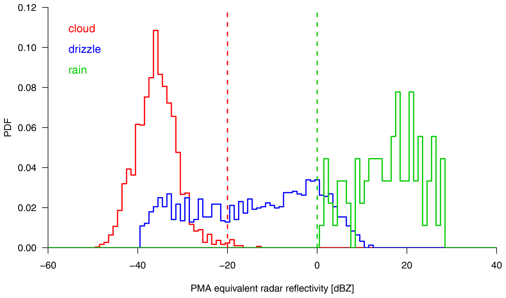
Figure 13Probability distribution function of equivalent radar reflectivities calculated for each ATR flight from the PMA particle size distribution for situations defined as cloud-only, drizzle-only or rain-only by PMA masks (based on LWC and cloud drop diameter; Sect. 3.4.2). The PMA measurements were performed along the R patterns flown around the cloud base level.
To assess the ability of these reflectivity thresholds to distinguish between cloud, drizzle and rain situations, we calculate the reflectivity ZPMA that would correspond to the drop size distribution of the PMA dataset. It is done using the T-matrix approach and accounting for the beam orientation and for the non-sphericity of large particles. For the smallest particles, ZPMA follows Rayleigh theory and is equal to 10 log 10(M6), where M6 is the sixth moment of the drop size distribution. The distribution of ZPMA values for situations classified by the PMA microphysical masks (based on LWC and D measurements; Sect. 3.4.2) as cloud-only, drizzle-only or rain-only shows that clouds and rain are mainly associated with reflectivities lower than −20 dBZ and larger than 0 dBZ, respectively (Fig 13), which supports the Zd and Zr thresholds used in the BASTALIAS dataset. Reflectivities between −20 and 0 dBZ are predominantly associated with drizzle. However, drizzle is associated with a broader range of reflectivities, and therefore its identification from reflectivity thresholds remains imperfect.
Since the sensitivity of the radar decreases as the distance from the aircraft increases, BASTA can only detect clouds within a limited distance from the aircraft; beyond this point, the radar can only detect drizzle or rain. The range over which the radar can possibly detect clouds () is determined by the distance at which the expected radar sensitivity corrected for attenuation equals Zd. In the trade-wind boundary layer conditions of EUREC4A, the radar could detect clouds over a maximum horizontal distance ranging from 1.5 to 3.5 km (2.2 km on average) for dBZ and from 2.9 to 6.2 km (3.8 km on average) for dBZ. On the other hand, drizzle and rain could be detected at any distance up to 12 km if there is no rain in the vicinity of the aircraft.
In parallel, the ALiAS lidar data at their original resolution (Level 1.5 data from Chazette et al., 2020) are analyzed to determine the horizontal lidar profile that corresponds to the molecular or aerosol backscatter, to estimate the noise level, and to detect the presence of clouds. The lidar cloud detection methodology used in the BASTALIAS dataset is inspired from that developed for the CALIPSO spaceborne lidar and the airborne LNG (Leandre Nouvelle Génération) lidar (Ceccaldi et al., 2013). Although derived from a different methodology, the lidar-only cloud mask of the BASTALIAS dataset is very consistent with that proposed by Chazette et al. (2020), showing the robustness of the cloud detection from lidar measurements. This information is then used to define a lidar pseudo cloud mask at the same space and time resolution as the radar information (for this purpose, each radar time is associated with the closest lidar observation in time). The cloud detection by the lidar is considered impossible beyond the distance from the aircraft () at which the lidar backscatter signal is completely extinguished or undistinguishable from noise. During EUREC4A, ranged from 0 to 8 km and was about 5 km on average.
Finally, the lidar and radar cloud masks are analyzed jointly to make a final classification of hydrometeors and a lidar–radar cloud mask (Fig. 12). The synergy between lidar and radar is illustrated by two examples of individual radar and lidar profiles along their horizontal line of sight (Fig. 14). In the first one, derived from a flight (RF05) associated with small very shallow clouds (“Sugar”; Table 3), the lidar detects three clouds in a row which are not detected by the radar; beyond (6.3 km), the backscatter signal is extinguished, and the cloud detection becomes impossible. In the second example, from RF11, the radar detects a cloud within the first kilometer, and then drizzle and rain. Wherever the radar detects drizzle or rain, the hydrometeors detected by the lidar are not considered to be a cloud in the cloud mask.
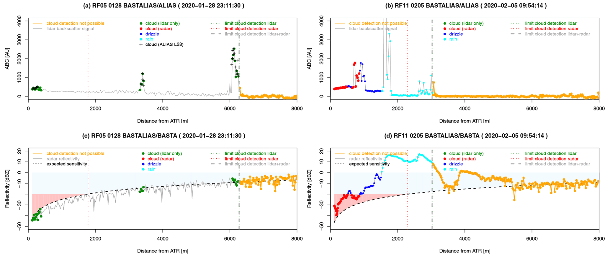
Figure 14Illustration of cloud, drizzle and rain detection by horizontal remote sensing using lidar–radar synergy. The maximum distances and over which cloud detection is possible with the ALiAS lidar or BASTA radar are indicated by vertical dash-dot green and dotted red lines, respectively. The range over which hydrometeor detection is no longer possible with radar or lidar is indicated in orange – it corresponds to the maximum of and . The classification of hydrometeors is reported on the lidar and radar signals: drizzle, rain, clouds detected only by lidar, and clouds detected by radar or both radar and lidar. On 28 January 2020 (RF05) at 23:11:30 UTC, the lidar (ALiAS; a) detects three areas of strong backscatter along its line of sight, while the radar (BASTA; c) detects no hydrometeor in the range (0–1.8 km) in which it could possibly detect clouds; the areas of strong lidar backscatter therefore correspond to the presence of thin clouds; beyond 6.3 km, the lidar signal is fully extinguished, and cloud detection is no longer possible. The cloud detection from the ALiAS Level 2 and Level 3 (L23) dataset (performed at a horizontal resolution of 15 m, as opposed to 25 m for BASTALIAS) and using the methodology described in Chazette et al. (2020)) is also reported (note that the ALiAS L23 times have to be shifted by −10 s to coincide with those of BASTALIAS). On 5 February 2020 (RF11) at 09:54:15 UTC, the lidar (b) measures four areas of strong backscatter and is fully attenuated beyond 3 km. The radar reflectivity (d) shows that the first area corresponds to the presence of clouds but that the following areas correspond to the presence of drizzle or rain (the cloud–drizzle and drizzle–rain transitions are defined by reflectivity thresholds, set here at −20 and 0 dBZ, respectively). In this case, no cloud can be detected beyond 3 km. This case is from an R pattern flown near the inversion level; no cloud mask is available from the ALiAS L23 dataset on R patterns above cloud base.
3.5.4 Vertical radar measurements (RASTA)
RASTA (RAdar SysTem Airborne) is an up-looking pulsed 95 GHz Doppler cloud radar with two antennas (zenith and up-backward, with an elevation of 66.7∘, 30 cm large; Table 9). The radar was dedicated to the characterization of cloud microphysics and dynamics. The radar was operated at 30 m resolution with a maximum range of 6 km at 1 s integration. Both Doppler moments (reflectivity and velocity) and spectrum are available. As for BASTA, the radar reflectivity is range-corrected and calibrated, and the background noise is removed using a thresholding technique based on the background noise characteristics. The derived mask is refined thanks to some image processing. The reflectivity is corrected for gaseous attenuation using colocated information from dropsonde temperature, humidity and pressure. Once the Doppler velocity is unfolded and corrected from the aircraft's motion and when backward and zenith antennas are simultaneously available, the vertical velocity and the along-track wind components of the cloud and precipitation wind are retrieved. Two antennas allow us to retrieve the two components of the wind in the plane defined by the two antennas.
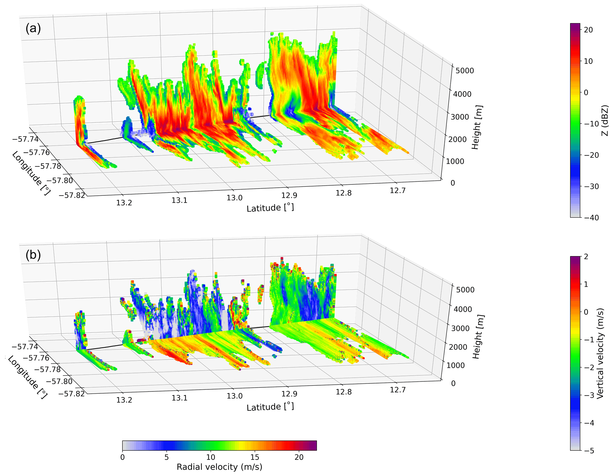
Figure 15(a) Reflectivity corrected for attenuation (dBZ) and (b) Doppler velocity (vertical component Vz and radial component Vx; m s−1) from the vertically pointing RASTA radar and from the horizontally pointing BASTA radar displayed as a function of height (for RASTA) or horizontal range (for BASTA), along a subcloud-layer leg during RF17 (from 09:06:09 to 09:20:03 UTC on 11 February 2020).
Level 2 data are distributed as a set of NetCDF files for the flights during which the radar was operating, and clouds were detectable with the radar (RF03, RF04, RF11 and RF12 plus all flights from RF13 to RF19). For all these flights but two (RF11 and RF12), two antennas were working (zenith and up-backward), which allows us to derive wind information (its radial component) in addition to cloud information. For RF11 and RF12, only one antenna (zenith) was working, and therefore the wind information is not available.
Figure 15 shows the reflectivity and Doppler velocity measured in the vertical and radial directions by the RASTA and BASTA radars during a leg of RF17. During this flight, the height of precipitating cloud tops could exceed 3 km. The vertical and radial reflectivity structures tend to reflect each other, suggesting a well-defined geometry (or aspect ratio) of the clouds. The vertical structure of the Doppler velocity from RASTA exhibits a maximum positive velocity near cloud top and negative velocities in the parts of clouds that are associated with falling hydrometeors (rain or drizzle).
3.6 Water stable isotopes (Picarro)
In addition to characterizing the meteorological, turbulent, microphysical, cloud and radiative properties of the atmosphere, the ATR measured the water-isotopic composition of the atmosphere using a customized fast-response cavity ring-down spectrometer from Picarro (version L2130-i). This effort took place as part of a wider EUREC4A-iso initiative involving multiple platforms and instruments (Stevens et al., 2021; Bailey et al., 2022). The rationale for isotopic measurements is that by quantifying the relative content of isotopically heavy (1H2H16O, 1HO) and light (1HO) water molecules in the atmosphere, it is possible to get information about the transport, mixing and phase changes of water. Isotopically heavy water molecules are associated with lower saturation vapor pressures and smaller diffusion velocities than their most abundant, lighter counterparts. Therefore, the three main components of the boundary layer moisture budget, namely ocean evaporation, convective drying and moistening by hydrometeor evaporation, carry a distinct stable water isotope signature (Risi et al., 2019). Specificities in the water vapor cycling associated with different mesoscale cloud organization patterns therefore result in characteristic isotopic fingerprints (Aemisegger et al., 2021b). Whether these fingerprints are primarily due to the local processing of water vapor in the marine boundary layer or result from the interaction with the large-scale flow is one of the questions to be addressed with water isotope tracers.
The isotopic composition of atmospheric water vapor on board the ATR was measured with a sampling frequency of 1 Hz (Table 9). The CRDS system uses laser absorption spectroscopy as a working principle: the different isotopic molecules having different rotational-vibrational energy level structure, they exhibit different transition frequencies in the near-infrared region of the spectrum. Three nearby absorption peaks in the near-infrared region (7199–7200 cm−1) corresponding to the three molecules (2H1H16O, 1HO and 1HO) are thus scanned by a laser in continuous-wave operation mode. Laser light is injected through a semi-transparent mirror into a 35 cm3 cavity with three mirrors in ring configuration (Crosson, 2008). A photodetector is placed behind another mirror and measures the light intensity leaking out of the cavity. The isotope concentration is determined by measuring the exponential ring-down time of the laser intensity after the laser source has been switched off. The higher the heavy isotope concentration, the faster the decay of the laser intensity.
In the ATR, a rearward-facing 30 cm long stainless-steel inlet with in. outer diameter was fitted to one of the front windows on the right-hand side of the aircraft (Fig. 7, Table 6). A 1.5 m heated PTFE line with 10 mm inner diameter was flushed with an inlet pump (KNF, HN022AN.18) at a rate of 13 L min−1. A filter (0.2 µm PTFE vent filter) was installed at the end of the inlet line to prevent particles from entering the laser spectrometer. A subsample from the inlet line was drawn into the instrument by a second pump (KNF, N920AP.29.18). The flow rate through the laser system was 280 mL min−1, and the residence time of the vapor sample in the system was 7–14 s, depending on the ambient pressure. This bottom-up residence time estimate from the gas flow setup was confirmed by a correlation analysis of the water vapor mixing ratio measured by the Picarro and the ATR’s dew point hygrometer. A time lag of between 6 and 15 s was found for the Picarro with synchronized computer clocks and was corrected in the post-processing. More details on the setup can be found in Bailey et al. (2022).
To assess the instrument's precision and drift, calibration gases were measured on the ground pre- and post-flight using a Picarro Standards Delivery Module (SDM). The high-precision liquid pumps of the SDM deliver a thin stream of liquid water of known isotopic composition into a vaporizer heated to 140 ∘C. In the vaporizer, the liquid water droplets are completely evaporated in a dry airstream, which was produced by pumping ambient air through a drying unit (Drierite) using a small air pump. In addition to the ground-based calibration runs, four in-flight calibrations were performed to assess the impact of aircraft vibrations on the precision of the measurements.
Recent studies have indicated that the precision of laser spectrometers in laboratory settings is comparable to the one of conventional isotope ratio mass spectrometer systems. However, for atmospheric field applications, the overall measurement uncertainty can result from a range of factors such as calibration, sensitivity to variations in water concentration and retention effects from the tubing (Aemisegger et al., 2012). A detailed post-processing procedure was therefore applied to account for these factors. In particular, a two-stage correction procedure following Weng et al. (2020) was applied at water vapor mixing ratios lower than 10 000 ppmv to correct for a known concentration bias in laser-spectrometric isotope measurements. The water vapor mixing ratio measurement from the CRDS system was calibrated based on a linear correction determined in the laboratory using a dew point generator. More details on the post-processing are available in Bailey et al. (2022). The dataset is distributed on AERIS as an ensemble of self-documented NetCDF files (Aemisegger et al., 2021a).
The ATR measured humidity, winds and clouds with multiple instruments based on different observation techniques. This redundancy and/or complementarity is an opportunity in several respects. It is an asset for the quality control of the data from each instrument and for the processing of combined datasets taking advantage of the complementarity of the instruments. It also allows the robustness and the statistical representativeness of the measurements to be assessed. This last point is particularly important for EUREC4A as the experiment was designed on the premise that the relationships between clouds and their environment could be characterized by combining measurements from several instruments and/or observing platforms that sample the atmosphere differently (Bony et al., 2017; Stevens et al., 2021).
The objective of this section is to verify this premise by comparing some of the main ATR measurements made by different instruments using different techniques and/or samplings. We also assess the consistency between the ATR measurements and the simultaneous dropsonde measurements (George et al., 2021) or BCO ground-based observations (Stevens et al., 2016).
4.1 Humidity
On board the ATR, humidity was measured by several instruments, but the WVSS-II sensor was considered as a reference for the calibration of the SAFIRE-CORE and SAFIRE-TURB datasets (Brilouet et al., 2021) because of its reliability and because it was the least affected by the presence of condensation or very dry air (Sect. 3.1.4). The Picarro CRDS measured water vapor with a similar sampling, and its data were calibrated on the basis of laboratory measurements (Sect. 3.6). During most ATR flights, HALO (or, on 11 February, the P-3) was flying circles of 200 km diameter at high altitude, measuring water vapor every 5 min and with a vertical resolution of about 10 m with Vaisala RD-41 dropsondes (George et al., 2021).

Figure 16Comparison for each ATR flight of the water vapor mixing ratio inferred (blue) from the SAFIRE-CORE dataset, (turquoise) from the Picarro dataset and (black) from the JOANNE dropsonde dataset. Panels (a), (b) and (c) are associated with different kinds of ATR patterns: R patterns (flown at cloud base), L patterns (flown in the subcloud layer) and S patterns flown near the sea surface, respectively. Note that the time axis is not linear. For the sake of readability, the markers associated with the different datasets are displayed with a slight horizontal offset. For a given flight, vertical bars represent the standard deviation of the mean values associated with the different segments of the same kind. The standard deviation of dropsonde data is computed on the basis of all the individual dropsondes launched during each ATR flight.
The comparison between these different measurements is presented in Fig. 16 for each ATR flight. For the SAFIRE-CORE and Picarro measurements, the mean and standard deviation of the water mixing ratio are calculated over all the “T-shortlegs” segments (Table 2) associated with a given kind of segment. Note that the legs flown around the middle and the top of the subcloud layer have been considered together because the subcloud layer is well mixed vertically (Albright et al., 2022). For dropsondes, they are calculated over all available Level 4 measurements in a layer comprised between the minimum altitude minus 50 m and the maximum altitude plus 50 m sampled by the ATR for a given pattern. Most of the sounding data within the EUREC4A circle are derived from HALO dropsondes; these data include a correction for the dry bias of these dropsondes (George et al., 2021).
For each flight and each pattern, the ATR measurements (SAFIRE-CORE and Picarro) generally exhibit a good agreement, in terms of both mean humidity and standard deviation: over the cloud base rectangles (R patterns), the mean discrepancy between the two datasets is 0.084 g kg−1 (0.63 %) and 0.21 g kg−1 (18.7 %) for the mean and standard deviation, respectively. Those differences are slightly larger on L patterns (0.27 g kg−1 or 1.85 % and 0.21 g kg−1 or 29.4 %, respectively) and on S patterns close to the surface (0.28 g kg−1 or 1.86 % and 0.13 g kg−1 or 33.5 %). The most notable exceptions occur on 11 February 2020 (RF17 and RF18), when the aircraft flew within or below precipitating clouds (Table 4): along a few legs, the quality of CRDS measurements was affected by the presence of cloud droplets or precipitation in the air inflow system.
The ATR measurements are also in good agreement with the dropsonde data, including when all the measurements show a small variability. Even the standard deviations show good agreement, which is somewhat surprising given the much larger domain sampled by the HALO measurements. However, ATR and HALO measurements disagree more during RF09 (on 2 February) and RF14 (on 7 February), when the cloud organization was very heterogeneous at the mesoscale (Table 3 reports a prominence of Flower and Fish organization on these days). During most of RF09 for instance, the ATR was sampling the clear-sky area surrounding cloud Flowers, while the dropsondes were sampling both clear-sky and cloudy areas. During RF06 (on 30 January), the variability in dropsonde measurements was very small because the corresponding HALO flight was much shorter and was associated with the launch of only 2 dropsondes in the ATR area (as opposed to about 36 for other flights).
This comparison suggests that despite their different sampling and observing techniques, the ATR and HALO generally measured statistically consistent variabilities in humidity around cloud base, within the subcloud layer and near the surface. The main discrepancies occurred when the scale of the cloud field organization was much larger than the scale of the area probed by the ATR. In these cases, the differences are likely to be representative of real spatial differences associated with different samplings.
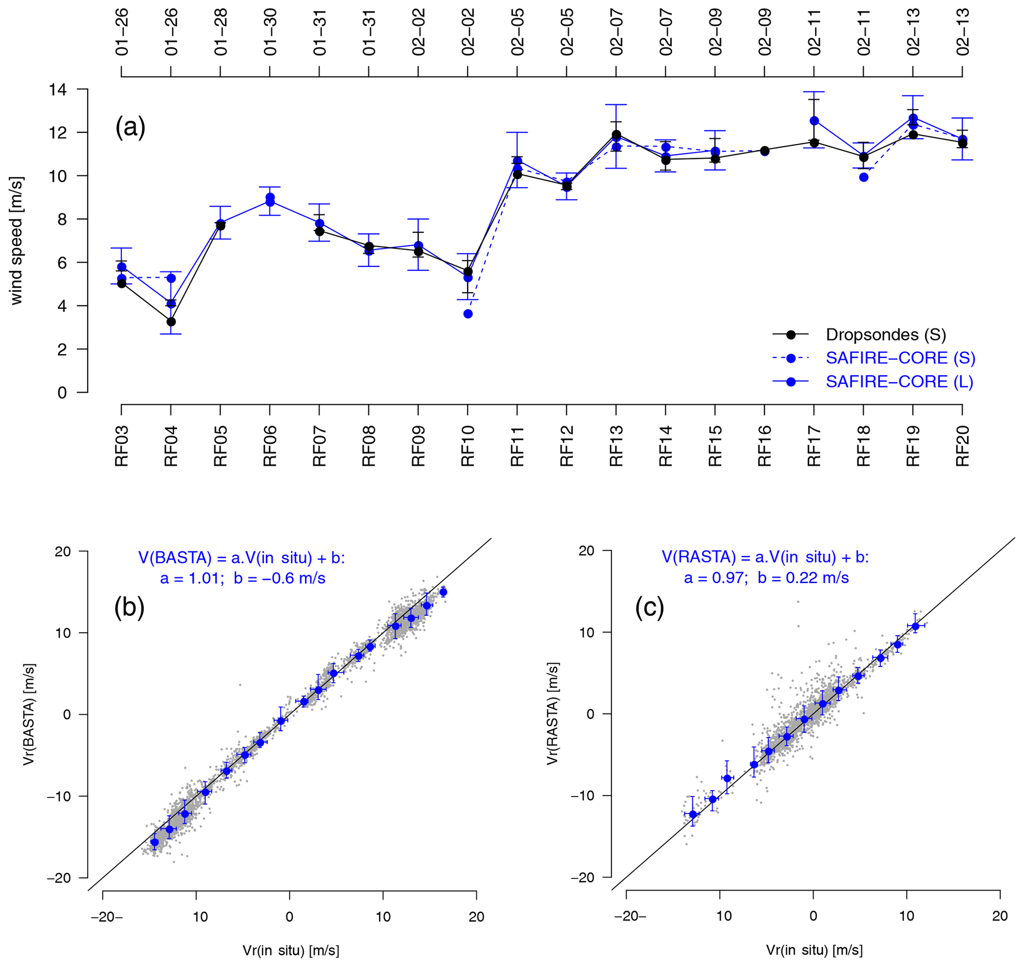
Figure 17(a) Comparison of the wind speed measured by the core instrumentation of the ATR (SAFIRE-CORE) in the subcloud layer with the near-surface wind measurements (at 60 m, close to the altitude of the near-surface legs of the ATR) from the HALO dropsondes. Each marker corresponds to the average value, for a given ATR flight, of the measurements collected over all the L patterns or S patterns of this flight, and the vertical bar represents the standard deviation among the different segments of a given pattern. Note that the time axis is not linear. (b, c) Comparison of the radial component of the wind (perpendicular to the aircraft) derived from the aircraft probes (SAFIRE-CORE dataset) with that inferred from (b) the horizontally staring BASTA Doppler radar at 25 m from the aircraft or (c) the vertically pointing RASTA Doppler radar at 60 m above the aircraft; the comparison is done for all R patterns flown at cloud base during the EUREC4A campaign (note that there were no wind measurements from RASTA from RF05 to RF12 and on RF20). Individual data points are shown in gray, and the binned relationship between the two measurements is shown in blue. Horizontal and vertical bars indicate the 25th–75th percentiles of the measurements within each bin of 2 m s−1.
4.2 Horizontal wind
The wind was measured both in situ using the aircraft probes (Sect. 3.1.2) and through remote sensing using the Doppler radars BASTA and RASTA (Sect. 3.5.2 and 3.5.4). In parallel, the wind was measured by dropsondes (George et al., 2021).
Figure 17 compares the wind speed measured in the subcloud layer or near the surface by the aircraft probes and by the HALO dropsondes at 60 m. The wind speed being quite similar near the surface and within the subcloud layer, we primarily consider the ATR measurements over L patterns because these patterns are available for every flight and are associated with longer measurements. Despite the different flight patterns of the ATR and HALO, the average wind speed measured by the two aircraft is very consistent: the dropsonde and ATR measurements correlate strongly (R=0.98) and differ by only 0.7±0.5 m s−1.
The two Doppler radars also measured the radial component of the horizontal wind along their line of sight. For BASTA, this information is retrieved on every flight, but for RASTA it is available only for RF03, RF04 and RF13 to RF19, when backward and zenith antennas were operating simultaneously. The radial component of the wind (perpendicular to the aircraft trajectory) derived from BASTA and RASTA along R patterns is compared to the horizontal wind measured by the aircraft probes and projected along the radars' line of sight (Fig. 17). For BASTA, the information is derived from the third gate (about 25 m from the aircraft), and for RASTA it is from the fourth gate (about 60 m above the aircraft). The radar Doppler and in situ measurements correlate strongly with each other (0.99 for the BASTA estimates, 0.94 for the RASTA estimates) and differ by −0.61 ± 1.22 and 0.24 ± 1.3 m s−1, respectively, over the whole campaign. The difference between BASTA estimates and in situ measurements reduces to 0 ± 1.22 m s−1 when RF17 and RF18 are not considered, showing that most of the uncertainty in wind retrieval from horizontal radar measurements occurs in the presence of rain. This bias arises because the vertical component of the wind has to be taken into account if the radar beams are not perfectly horizontal, which requires the terminal speed of the hydrometeors to be accounted for. This might be corrected in future versions of the BASTA dataset. The radar Doppler measurements also agree with the HALO radiosonde measurements of the horizontal wind at the same height projected along the line of sight of the radars (not shown); on average over the campaign, the BASTA and RASTA estimates differ from the HALO dropsonde data by −0.45 and +1 m s−1, respectively.
In summary, the horizontal wind measurements of the ATR are consistent with each other and with the dropsonde measurements made along the EUREC4A circle. It confirms that the flight strategy resulted in a good statistical sampling of the lower-tropospheric wind.
4.3 Cloud base cloud fraction
One of the original motivations for the EUREC4A campaign was to test the mixing–desiccation mechanism by which increased convective mixing in the lower troposphere dries the atmosphere around cloud base and reduces cloudiness (Bony et al., 2017). This mechanism, which has been shown to contribute to the strong positive feedback of low clouds and the high climate sensitivity of a number of climate models, remains to be tested observationally. Such a test requires measuring the cloud fraction at cloud base CFb together with the lower-tropospheric mixing from convection and larger-scale vertical motions.
Reflecting the view that clouds are bodies interacting with radiation, collections of particles and a particular state of atmospheric water (Siebesma et al., 2020), we estimate CFb in different ways, using various observations ranging from lidar and radar remote sensing to in situ microphysical measurements (defining the cloud mask either from the cloud particle properties directly or from the equivalent radar reflectivity calculated from these properties) and high-frequency humidity measurements.
Using horizontal lidar–radar measurements from ALiAS and BASTA together with the BASTALIAS cloud detection algorithm described in Sect. 3.5.3, we diagnose the cloud fraction within the rectangle area associated with the R patterns flown at cloud base: for each R pattern, we divide the total number of points classified as “cloudy” along the instruments' line of sight by the total number of points where a cloud detection is possible. The resulting time series of CFb is shown in Fig. 18, which uses a reflectivity threshold for the cloud–drizzle transition of −20 dBZ. Using a different threshold (−17 or −15 dBZ) makes very little difference in the time series (not shown). CFb is small on average (3.5 %), but it ranges from 0 % to 6 % across flights. Minima in CFb occurred during RF09 and RF14, when the ATR was flying within the clear-sky area of a field of “cloud Flowers” organized at the mesoscale (Table 4).
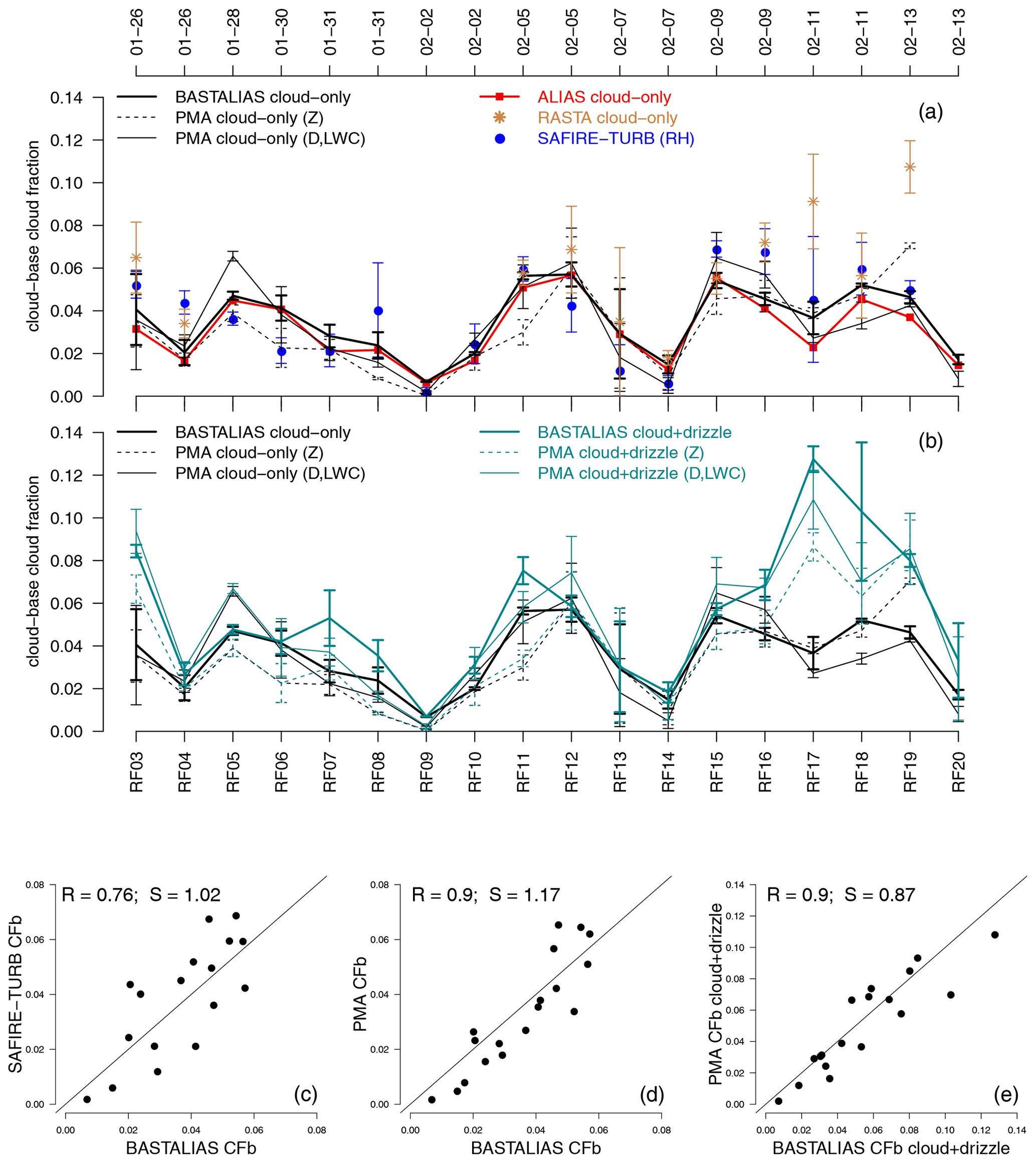
Figure 18(a) Cloud base cloud fraction (CFb) inferred from ATR observations across or along the R patterns flown at cloud base: from horizontal radar–lidar remote sensing (BASTALIAS), from horizontal lidar only (ALiAS), from in situ microphysical measurements (PMA) using an hydrometeor classification based either on (D, LWC) or on reflectivities (Z) inferred from the particle size distribution, from in situ humidity measurements at the turbulence scale (RH from SAFIRE-TURB), and from the vertically pointing RASTA radar. (b) Comparison of the fractional area covered by “clouds only” (in black) or by “clouds+drizzle” (in color) inferred either from the BASTALIAS lidar–radar dataset or from the PMA dataset using both types of hydrometeor classification. Note that the time axis is not linear. (c, d, e) Correlation (R) and linear regression coefficient (S) between the CFb estimates derived from different ATR datasets.
Most of the cloud fraction (from 60 % to 100 %) is composed of clouds which were detected by the lidar only (Fig. 18). As explained in Sect. 3.5.3, it is because a large proportion of clouds in the trades are small (a few hundred meters) and optically thin (especially at cloud base, where the liquid water content is small) and because in the trade-wind boundary layer, horizontal radar measurements can only detect clouds over a range of 2–3 km from the aircraft, while horizontal lidar measurements can detect clouds over a distance at least twice as large.

Figure 19Comparison of the ATR isotope measurements below 400 m (in blue) with the ground-based measurements from the Barbados Cloud Observatory (BCO) during each ATR flight (in black). The comparison is done (from top to bottom) for δ18O, δ2H, d excess (‰), specific humidity (g kg−1) and the length of measurements (expressed in minutes).
Table 10Mean values and standard deviations over all flights for the measurements made by the Picarro onboard the ATR and at the BCO during the ATR flights, as well as the Pearson correlation between the two datasets.
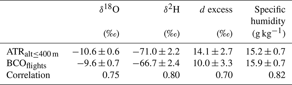
Using reflectivities at the fifth gate (i.e., about 90 m above the aircraft), and a threshold of −20 dBZ to distinguish clouds from drizzle, a cloud fraction can also be derived from the vertically pointing cloud radar measurements (RASTA; Sect. 3.5.4). The CFb estimates from RASTA are in good agreement with those from BASTALIAS, except on RF17 and RF19, during which RASTA measurements seem to be dominated by rain.
A cloud fraction estimate can also be diagnosed from in situ measurements of cloud microphysics (Sect. 3.4.2) using two methods. The first one consists of using the PMA hydrometeor masks defined as LWC ≥0.010 g m−3 and D<100 µm and the drizzle mask as µm. We then compute a cloud fraction along the aircraft trajectory as the ratio between the number of points classified as “cloud-only” over the total number of valid measurements. Although the sampling along the aircraft trajectory is much less extensive than that of horizontal lidar–radar measurements, the time evolution of the CFb derived from PMA data is highly correlated (R=0.90) with that from BASTALIAS (Fig. 18). The presence of drizzle can make the definition of the cloud base cloud fraction ambiguous as drizzle can fall within the cloud base. For this reason, we also compute a cloud fraction considering both clouds and drizzle, diagnosed either from BASTALIAS data or from PMA cloud microphysical data. The cloud-plus-drizzle fraction differs from the cloud-only fraction mostly on 11 February, during which the ATR flew during nighttime (RF17) or in the morning (RF18) in the presence of cloud Flowers and a strong ascending motion in the free troposphere (Sect. 2.5). However, even in the presence of drizzle and rain, estimates from the two measurements are very consistent with each other (R=0.90; Fig. 18).
Finally, recognizing that clouds occur in saturated (or, in the presence of sea salt, nearly saturated with respect to pure water saturation) conditions, it is possible to define a pseudo cloud fraction from the high-frequency (25 Hz), small-scale (4 m) measurements of relative humidity: using the SAFIRE-TURB dataset, we reconstruct high-resolution time series of humidity mixing ratio, temperature and then relative humidity by adding the turbulent fluctuations in each variable measured over stabilized segments (T-shortlegs) to the mean of each segment (Fig. 6 herein, Brilouet et al., 2021). Then, by counting the proportion of measurements having a relative humidity exceeding a threshold RHc, we define a pseudo cloud fraction from the SAFIRE-TURB dataset. The time series of CFb obtained with this method using a threshold RHc=0.98 is in good agreement and correlates well with the cloud fraction estimated from BASTALIAS (R=0.76) or PMA data (R=0.71). The best correlation with BASTALIAS and PMA data is obtained during the second half of the campaign (after RF09), when the high-frequency measurements of humidity were of the best quality (Brilouet et al., 2021).
The values of CFb derived from the different datasets obviously depend to some extent on the thresholds used to define cloudy conditions. However, sensitivity tests suggest that the high correlation among the different estimates remains for a range of threshold values. Considering the diversity of measurement techniques (in situ microphysical and turbulent measurements, horizontal lidar–radar measurements, vertical radar measurements) and spatial samplings (rectangle perimeter or rectangle area) leading to consistent results, the CFb estimates from the ATR can be considered to be robust.
4.4 Water-isotopic composition
To assess the consistency of isotopic data between the ATR Picarro dataset and the ground-based measurements from the BCO (Fig. 19), we select the data collected at altitudes lower than 400 m (this height is well below cloud base for all flights and contains the ground-based measurements at the airport) and compute the mean value for each flight (ATRalt≤400 m). The BCO data are averaged over each flight’s period (BCOflights). The vapor sampled by the Picarro onboard the ATR was drier (−0.7 g kg−1) and more depleted (−1 ‰ in δ18O ‰ and −4.3 ‰ in δ2H) than at the BCO (Table 10). The d excess was nearly identical except for RF04, RF07 and RF08, for which the d excess at the BCO was lower. Similar differences between the BCO and the R/V Atalante were recorded during a comparison stop offshore the BCO (Gilles Reverdin, personal communication, 2022). A possible explanation for the observed differences could be the effect of sea spray evaporation due to the wave activity at the cliff in front of the BCO that enriches and moistens the air close to the land-based site. The flight-to-flight isotope variability recorded by the ATR agrees well with the one observed at the BCO: correlations between ATRalt≤400 m and BCOflights range from 0.7 to 0.82 (Table 10). Due to their spatial separation, the instruments did not measure the exact same air or, if so, due to advection, with a time lag. Therefore, the qualitative and quantitative match between the datasets suggests that the measurement are of good quality and that distinct mesoscale environmental conditions were measurable during the different research flights.
All the datasets discussed in this paper are available on the EUREC4A database of AERIS (https://eurec4a.aeris-data.fr, last access: 19 December 2021), and their respective DOIs are summarized in Table 11.
Bony et al. (2021)Fildier et al. (2021b)CNRM/TRAMM et al. (2021)CNRM/TRAMM (2020a)CNRM/TRAMM (2020b)Cornet and JIANG (2021)Coutris and Schwarzenboeck (2021a)Coutris and Schwarzenboeck (2021b)Coutris (2021)Coutris and Ehses (2021)Le Gac et al. (2021)Delanoë et al. (2021)Caudoux et al. (2021)Bailey et al. (2022)Aemisegger et al. (2021a)Brilouet et al. (2021)Lothon and Brilouet (2020)Chazette et al. (2020)Chazette (2020a)Chazette et al. (2020)Chazette (2020b)Chazette et al. (2020)Chazette (2020c)
The EUREC4A field campaign, which aims at better understanding the link between clouds and circulation in the region of the trades, based its core experimental strategy on the coordinated operations of two research aircraft (Bony et al., 2017; Stevens et al., 2021): the French ATR aircraft flying in the lower troposphere and the German HALO aircraft flying at an altitude of 9–10 km. This paper presents the EUREC4A's ATR operations and presents the 19 ATR flights (totaling approximately 82 flight hours) that took place from 25 January to 13 February 2020 over the tropical Atlantic Ocean, east of Barbados.
The ATR mission focused on characterizing the thermodynamic, dynamical, microphysical, turbulent and cloud properties of the lower atmosphere. One of its specific roles was to measure the cloud fraction around cloud base to help test low-cloud feedback mechanisms. For this and other purposes, the ATR was equipped with a rich and extensive instrumentation composed of in situ sensors, radiometers and active remote sensing. Eighteen coordinated research missions followed a repeated flight plan consisting of rectangles (or R patterns) flown at cloud base or cloud top, L legs flown within the subcloud layer (L patterns), straight legs flown 60 m above the sea surface (S patterns), and ferry legs flown in the lower free troposphere above clouds.
The first part of this paper presents the ATR operations, the flight patterns and the flight segmentation (summarized in a collection of YAML files). It also shows that during its 19 missions, the ATR sampled very contrasted environmental conditions.
The second part of this paper presents the ATR instrumentation used during EUREC4A: three temperature sensors, five humidity sensors, two broadband radiometers, an infrared spectrometer, two visible cameras, six microphysical probes, a horizontally staring backscatter lidar, two Doppler cloud radars (one pointing horizontally and one pointing vertically) and a laser spectrometer for water isotopologues. The paper presents the different instruments, highlighting the complementarity that results from their different working principles. Then it presents the main aspects of the data processing and the datasets produced from the different measurements: the core thermodynamical, dynamical and radiative measurements (SAFIRE-CORE, SAFIRE-RADIATION, SAFIRE-CLIMAT, SAFIRE-CAMERA); turbulence measurements (SAFIRE-TURB; Brilouet et al., 2021); aerosol (UHSAS) and cloud microphysical (PMA) measurements; horizontal lidar measurements (ALiAS; Chazette et al., 2020); horizontal radar (BASTA) and lidar–radar (BASTALIAS) measurements; vertical radar measurements (RASTA); and water-isotopic measurements (Picarro).
Finally, the paper assesses the consistency among the different ATR measurements and between the ATR measurements and those performed by other instruments on different platforms such as HALO or the BCO.
The large variability in the aerosol load in the atmosphere (ranging from 50 to more than 500 cm−3) is measured consistently by the ALiAS lidar and by UHSAS microphysical probes (Sect. 3.4.1 and 3.5.1). The measurements of humidity, wind and cloud base cloud fraction also exhibit a good consistency among the different ATR datasets. The mean specific humidity measured by in situ sensors differs from that measured by the ATR Picarro laser spectrometer by less than 0.1 g kg−1 at cloud base and by less than 0.3 g kg−1 within the subcloud layer; larger disagreements occur on RF17 and RF18, when the Picarro measurements were impacted by cloud droplets and precipitation in the air inflow system. Estimates of the radial component of the wind from the Doppler cloud radars are in good agreement with the aircraft probe measurements, with a discrepancy of m s−1 for BASTA and 0.24 ± 1.3 m s−1 for RASTA. Finally, a cloud base cloud fraction was estimated for the first time from horizontal lidar–radar measurements (BASTALIAS), and other estimates were derived from in situ microphysical or turbulent measurements along the aircraft trajectory. These different estimates are in good agreement with each other (correlations of 0.76 and 0.91 between BASTALIAS and SAFIRE-TURB or PMA estimates, respectively). The cloud base fractional areas associated with “clouds plus drizzle” estimated either from BASTALIAS or from PMA datasets are also consistent with each other (correlation of 0.92). The good consistency obtained despite fundamentally different measurement techniques and different atmospheric samplings (in situ sensors sample the atmosphere along the aircraft line of flight, i. e. along the rectangle perimeter, while horizontal lidar–radar remote sensing samples the interior of the rectangle) shows that the ATR measurements of humidity, wind and cloud base cloud fraction are robust.
The ATR measurements of humidity and winds exhibit a good consistency with HALO dropsonde measurements: the wind measurements from the ATR and from HALO are highly correlated (R=0.98) and differ by only 0.7 ± 0.5 m s−1; the ATR humidity measurements are also in good agreement with the dropsonde data, in terms of both mean and variability. It shows that the measurements made by HALO and the ATR are consistently representative of the explored area, despite the complexity of the cloud organization and its inner heterogeneity.
These results thus verify two premises which were at the basis of the EUREC4A experimental strategy: (1) it is possible to measure the cloud base cloud fraction in a robust way, and (2) the repeated flight patterns of HALO and the ATR allow us to sample the atmosphere statistically in a consistent way, except when the cloud field is organized on a scale much larger than the scale of the ATR flight pattern (which only occurred twice out of the 18 flights). It is therefore legitimate to use observations from the different EUREC4A platforms together to carry out process studies. The availability of data from the ATR and other platforms together with the large diversity of environmental conditions and clouds encountered during the campaign should thus make it possible to better understand the physical processes underlying the cloud–circulation interactions in the trades.
| Abbreviation | Definition |
| 2D-S | 2D stereo |
| ABC | Apparent backscatter coefficient |
| AEC | Aerosol extinction coefficient |
| ALiAS | Airborne Lidar for Atmospheric Studies |
| BASTA | Bistatic Radar System for Atmospheric |
| Studies | |
| BCO | Barbados Cloud Observatory |
| CDP | Cloud droplet probe |
| CRDS | Cavity ring-down spectrometer |
| ERA5 | ECMWF Reanalysis 5th Generation |
| EUREC4A | Elucidating the role of cloud–circulation |
| coupling in climate | |
| FCDP | Fast cloud droplet probe |
| FMCW | Frequency-modulated continuous-wave |
| FSSP | Forward-scattering spectrometer probe |
| GOES | Geostationary Operational Environmental |
| Satellite | |
| GPS | Global positioning system |
| HALO | High Altitude and LOng Range Research |
| Aircraft | |
| INS | Inertial navigational system |
| KH20 | Krypton hygrometer |
| LCL | Lifting condensation level |
| LNG | Leandre Nouvelle Génération |
| LWC | Liquid water content |
| MSD | Mass size distribution |
| MVD | Median volume diameter |
| NOAA | National Oceanic and Atmospheric |
| Administration | |
| NT | Total particle concentration |
| PMA | Microphysics Airborne Platform |
| PSD | Particle size distribution |
| RASTA | RAdar SysTem Airborne |
| RF | Research flight |
| RH | Relative humidity |
| RSS | Regional Security System |
| SAFIRE | Service des Avions Français Instrumentés |
| pour la Recherche en Environnment | |
| UAV | Unmanned aerial vehicle |
| UHSAS | Ultra-high-sensitivity aerosol |
| spectrometer | |
| VDR | Volume depolarization ratio |
| WVSSII | Water Vapor Sensing System version two |
Satellite animations were made to visualize the cloud scenes sampled by the ATR and other platforms during the campaign. Geostationary images shown here are from the GOES-16 visible channel during daytime (channel 2) and infrared channel during nighttime (channel 13). They are retrieved at 1 min time increments and 500 m resolution during daytime and 2 km resolution during nighttime. The code is modular (Fildier et al., 2021a), and it can be used to generate movies with any combination of platforms making measurements in the region captured by the mesoscans (8.2457–17.9343∘ N, 50.1323–61.3010∘ W). It can also include the trajectory of the radiosondes and dropsondes launched. Here, movies are restricted to the ATR track in the domain 11.8–14.8∘ N, 57–60∘ W. The source code to generate GOES movies is archived at https://doi.org/10.5281/zenodo.4777954 (Fildier et al., 2021a) and in the GitHub repository (https://github.com/bfildier/EUREC4A_movies, last access: 19 December 2021).
Figures and show the horizontal and vertical trajectories of each ATR flight.
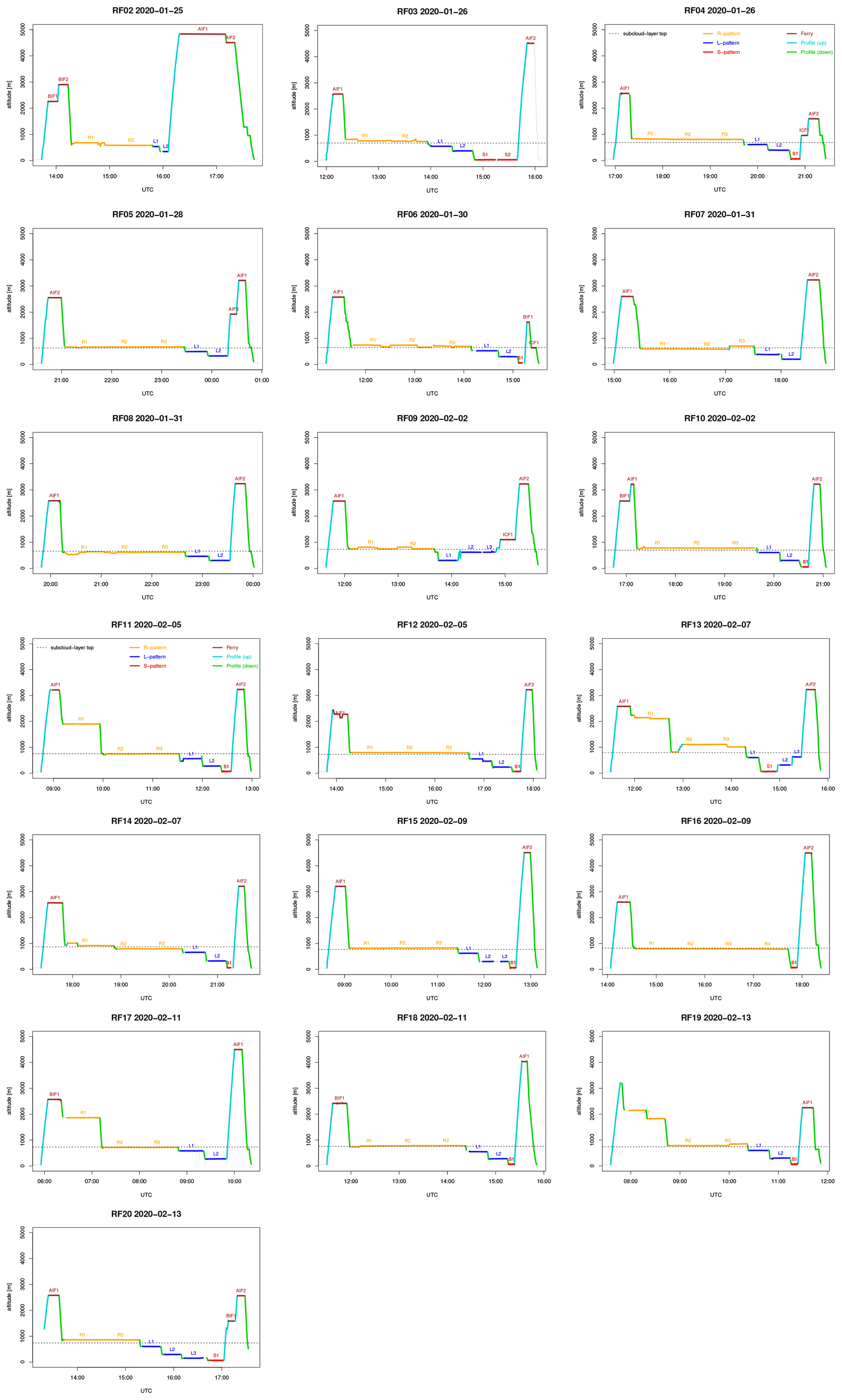
Figure C1Vertical trajectories of each ATR flight, with the main patterns highlighted in color. R patterns at cloud base and/or cloud top (orange), L patterns in the subcloud layer (blue), S patterns near the sea surface (red), ferry legs (black), and upward and downward profiles (turquoise). Also reported (dashed line) is the subcloud-layer top height diagnosed from dropsondes (Table 3).
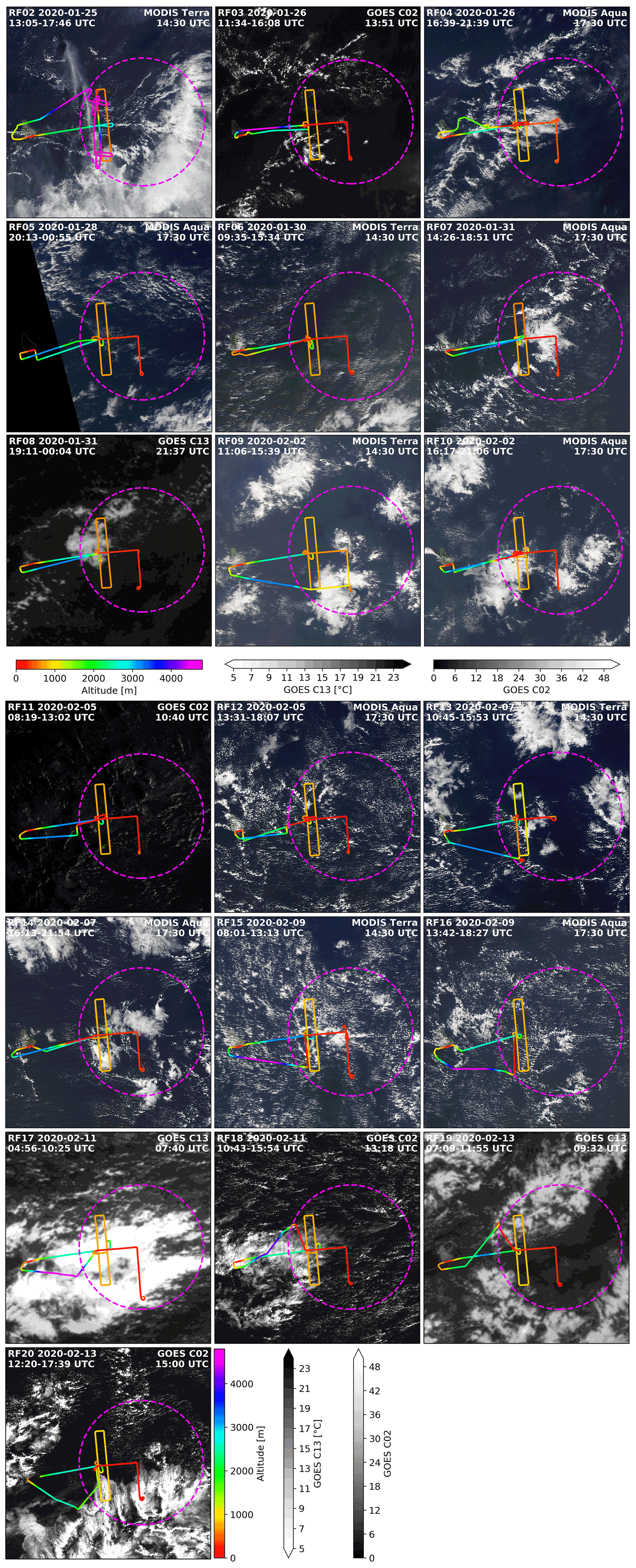
Figure C2Longitude–latitude trajectories of the ATR colored by the flight altitude. For repetitive flight patterns (e.g., the rectangles), only the last repetition is visible due to the overlap. The dashed circle shows the EUREC4A circle along which HALO was flying. The ATR tracks are shown on top of a satellite snapshot of the domain (11.8–14.8∘ N, 57–60∘ W) derived from either MODIS Terra/Aqua images (when available during the flight) or GOES-16 (using either the C02 (visible) or C13 (infrared) channel) at about mid-flight time.
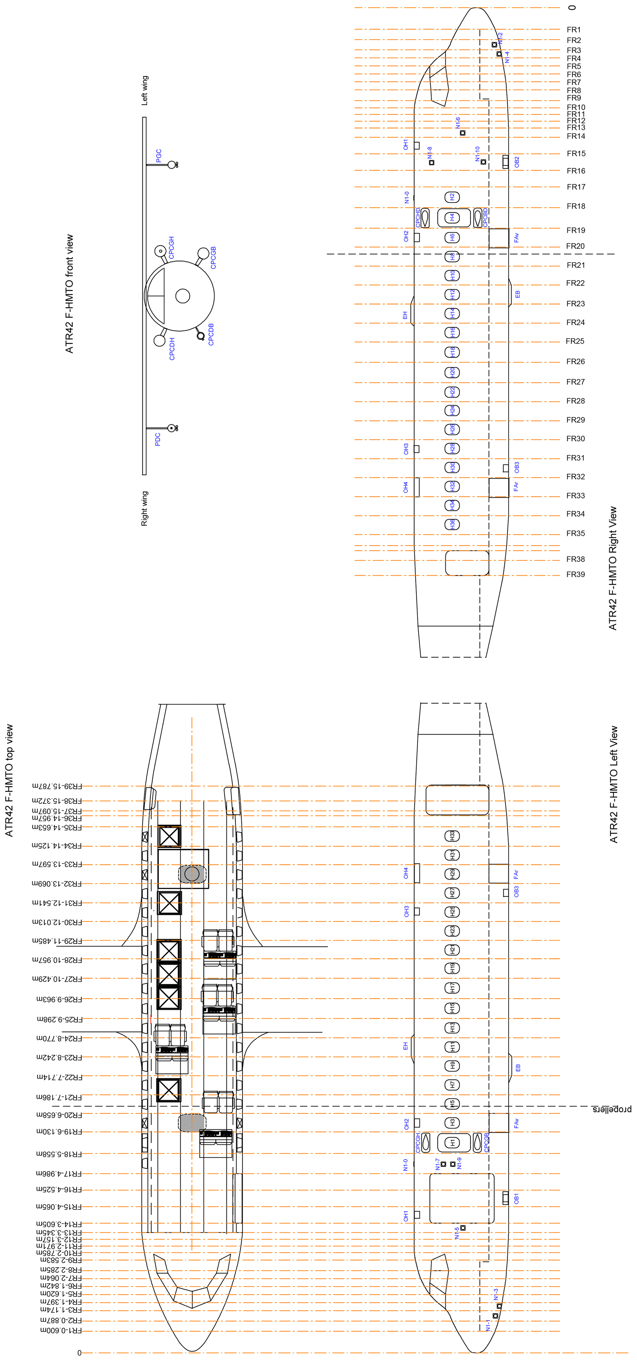
The people responsible for the processing of the different ATR datasets are listed in Table 11. SB led the ATR team and coordinated the scientific operations with ML, JD and BS. JCC and JPD led the SAFIRE operations with the support of AB. PC, CF, JT and AB were responsible for the lidar measurements; JD, CLG and CC for the radar measurements; ML, PEB and SAFIRE/TRAMM (JCE and PR) for the core and turbulence measurements; AS, PC and CG for the microphysical measurements; FA and LV for the isotopic measurements; and CC and TJ for the camera measurements. RV was responsible for the ground support with the help of JV and NR. TA, HB, MC, LG, TJ, ClL, JL, TP, FP, KS and GV were the technicians and engineers who took care of the integration and the operation of the instruments on board the ATR. JFB, GS, DD and ChL flew the ATR. BF and LTP produced the GOES animations with the help of Hauke Schulz. Figures 2a and were prepared by LV; Fig. 3 by RV; Figs. 2b, 7 and D1 by JCE and LG, Fig. 8 by CC; Figs. 12 and 15 by JD; Fig. 16 by PEB, ALA and FA; and Fig. 19 by FA. Tables 3 and 4 have been prepared by JV and Table 10 by LV. SB prepared all other tables and figures; analyzed the consistency among the different ATR datasets; and wrote the paper with ML, JCE, PC and JD, with contributions from FA, RV and JV. All authors edited the manuscript. SB and BS conceived the strategy and led the EUREC4A field campaign.
The contact author has declared that neither they nor their co-authors have any competing interests.
Publisher’s note: Copernicus Publications remains neutral with regard to jurisdictional claims in published maps and institutional affiliations.
This article is part of the special issue “Elucidating the role of clouds–circulation coupling in climate: datasets from the 2020 (EUREC4A) field campaign”. It is not associated with a conference.
The Caribbean Regional Security System (RSS), especially George Harris and Calvert Herbert, are gratefully acknowledged for hosting the ATR and the ATR team in Barbados in the best conditions during the EUREC4A experiment. The authors thank David Farrell, principal of the Caribbean Institute for Meteorology and Hydrology (CIMH), and Don Chee-A-Tow, honorary consul of France in Barbados, for their precious support during the preparation and the realization of the campaign. The Department of Civil Aviation in Barbados, Andrea Hausold from DLR, the British Twin Otter team, the German HALO team, the NOAA P3 team and the Boreal team are also gratefully acknowledged for their help, constructive spirits and cooperation during the airborne operations. The authors are grateful to Caroline Muller, Heike Kalesse, Katharina Baier, Johannes Röttenbacher, Friedhelm Jansen, Sabrina Schnitt, Geet George, Martin Wirth, Silke Gross and Stefan Kinne for their help with ground support during the ATR operations and to Vincent Douet and Karim Ramage for their help in distributing the ATR datasets on the EUREC4A database. The EUREC4A database is maintained by the French national center for atmospheric data and services AERIS.
This project was funded by the European Research Council (ERC) under the European Union’s Horizon 2020 research and innovation program (EUREC4A advanced grant no. 694768). It also received support from the French National Center for Space Studies (CNES) through the EECLAT proposal and from Météo-France. Leonie Villiger and Franziska Aemisegge received funding from the Swiss National Science Foundation (grant no. 188731). The cloud microphysics data were collected using instruments from the French Airborne Measurement Platform, a facility partially funded by CNRS/INSU and CNES.
This paper was edited by Silke Gross and reviewed by Alan Blyth and one anonymous referee.
Aemisegger, F., Sturm, P., Graf, P., Sodemann, H., Pfahl, S., Knohl, A., and Wernli, H.: Measuring variations of δ18O and δ2H in atmospheric water vapour using two commercial laser-based spectrometers: an instrument characterisation study, Atmos. Meas. Tech., 5, 1491–1511, https://doi.org/10.5194/amt-5-1491-2012, 2012. a
Aemisegger, F., Dütsch, M., Rösch, M., and Villiger, L.: Calibrated stable water vapour isotope measurements on board the ATR-42 during EUREC4A, Aeris [data set], https://doi.org/10.25326/244, 2021a. a, b
Aemisegger, F., Vogel, R., Graf, P., Dahinden, F., Villiger, L., Jansen, F., Bony, S., Stevens, B., and Wernli, H.: How Rossby wave breaking modulates the water cycle in the North Atlantic trade wind region, Weather Clim. Dynam., 2, 281–309, https://doi.org/10.5194/wcd-2-281-2021, 2021b. a
Albright, A. L., Bony, S., Stevens, B., and Vogel, R.: Observed subcloud layer moisture and heat budgets in the trades, J. Atmos. Sci., in revision, 2022. a
Bailey, A., Aemisegger, F., Villiger, L., Los, S. A., Reverdin, G., Quiñones Meléndez, E., Acquistapace, C., Baranowski, D. B., Böck, T., Bony, S., Bordsdorff, T., Coffman, D., de Szoeke, S. P., Diekmann, C. J., Dütsch, M., Ertl, B., Galewsky, J., Henze, D., Makuch, P., Noone, D., Quinn, P. K., Rösch, M., Schneider, A., Schneider, M., Speich, S., Stevens, B., and Thompson, E.: Isotopic measurements in water vapor, precipitation, and seawater during EUREC4A, Earth Syst. Sci. Data Discuss. [preprint], https://doi.org/10.5194/essd-2022-3, in review, 2022. a, b, c, d, e
Bansemer, A.: A Multi-Instrument Comparison of Small Ice Particle Size Distributions Measured from Aircraft, 15th Conference on Cloud Physics/15th Conference on Atmospheric Radiation, 9–13 July 2018, Vancouver, BC, 9–13, 2018. a
Bony, S. and Stevens, B.: Measuring Area-Averaged Vertical Motions with Dropsondes, J. Atmos. Sci, 76, 767–783, 2019. a
Bony, S., Stevens, B., Ament, F., Bigorre, S., Chazette, P., Crewell, S., Delanoë, J., Emanuel, K., Farrell, D., Flamant, C., Gross, S., Hirsch, L., Karstensen, J., Mayer, B., Nuijens, L., Ruppert, J. H., Sandu, I., Siebesma, P., Speich, S., Szczap, F., Totems, J., Vogel, R., Wendisch, M., and Wirth, M.: EUREC4A: A field campaign to Elucidate the Couplings between Clouds, Convection and Circulation, Surv. Geophys., 36, 1529–1568, 2017. a, b, c, d, e, f
Bony, S., Brilouet, P.-E., and Aemisegger, F.: SAFIRE ATR42: Flights segmentation, Aeris [data set], https://doi.org/10.25326/315, 2021. a
Brilouet, P.-E., Lothon, M., Etienne, J.-C., Richard, P., Bony, S., Lernoult, J., Bellec, H., Vergez, G., Perrin, T., Delanoë, J., Jiang, T., Pouvesle, F., Lainard, C., Cluzeau, M., Guiraud, L., Medina, P., and Charoy, T.: The EUREC4A turbulence dataset derived from the SAFIRE ATR 42 aircraft, Earth Syst. Sci. Data, 13, 3379–3398, https://doi.org/10.5194/essd-13-3379-2021, 2021. a, b, c, d, e, f, g, h, i, j, k, l, m, n
Brogniez, G., Pietras, C., Legrand, M., Dubuisson, P., and Haeffelin, M.: A High-Accuracy Multiwavelength Radiometer for In Situ Measurements in the Thermal Infrared. Part II: Behavior in Field Experiments, J. Atmos. Ocean. Tech., 20, 1023–1033, https://doi.org/10.1175/1520-0426(2003)20<1023:AHMRFI>2.0.CO;2, 2003. a
Buck, A.: The Lyman-alpha absorption hygrometer. Moisture and Humidity: Measurement and Control in Science and Industry, Tech. rep., Instrum. Soc. Amer., Research Triangle Park, NC, 411–436, 1985. a
Cai, Y., Montague, D. C., Mooiweer-Bryan, W., and Deshler, T.: Performance characteristics of the ultra high sensitivity aerosol spectrometer for particles between 55 and 800nm: Laboratory and field studies, J. Aerosol Sci., 39, 759–769, https://doi.org/10.1016/j.jaerosci.2008.04.007, 2008. a, b
Campbell, G. S., Gauthier, R. V., and Tanner, B. D.: Krypton hygrometer, https://www.osti.gov/biblio/6337278 (last access: 25 April 2022), 1985. a
Canut, G., Couvreux, F., Lothon, M., Pino, D., and Saïd, F.: Observations and Large-Eddy Simulations of Entrainment in the Sheared Sahelian Boundary Layer, Bound.-Lay. Meteorol., 142, 79–101, https://doi.org/10.1007/s10546-011-9661-x, 2012. a
Caudoux, C., Bony, S., and Delanoë, J.: SAFIRE ATR42: RASTA L2 dataset, Aeris [data set], https://doi.org/10.25326/313, 2021. a
Ceccaldi, M., Delanoë, J., Hogan, R. J., Pounder, N. L., Protat, A., and Pelon, J.: From CloudSat-CALIPSO to EarthCare: Evolution of the DARDAR cloud classification and its comparison to airborne radar-lidar observations, J. Geophys. Res., 118, 7962–7981, https://doi.org/10.1002/jgrd.50579, 2013. a
Charoy, T.: Mesure rapide de l'humidité dans l'atmosphère, Tech. rep., Arts et Métiers ParisTech, Bordeaux-Talence, internal report of an engineering internship made at the Laboratoire d'Aérologie de l'Observatoire Midi-Pyrénées and SAFIRE, 2015. a
Chazette, P.: SAFIRE ATR42: Lidar ALiAS – level 1 and 1.5, Aeris [data set], https://doi.org/10.25326/57, 2020a. a
Chazette, P.: EUREC4A – ATR-42 – Lidar ALiAS – level 2 and 3 aerosol products, Aeris [data set], https://doi.org/10.25326/59, 2020b a
Chazette, P.: EUREC4A – ATR-42 – Lidar ALiAS – level 2 and 3 cloud products, Aeris [data set], https://doi.org/10.25326/58, 2020c. a
Chazette, P., Dabas, A., Sanak, J., Lardier, M., and Royer, P.: French airborne lidar measurements for Eyjafjallajökull ash plume survey, Atmos. Chem. Phys., 12, 7059–7072, https://doi.org/10.5194/acp-12-7059-2012, 2012. a
Chazette, P., Totems, J., Baron, A., Flamant, C., and Bony, S.: Trade-wind clouds and aerosols characterized by airborne horizontal lidar measurements during the EUREC4A field campaign, Earth Syst. Sci. Data, 12, 2919–2936, https://doi.org/10.5194/essd-12-2919-2020, 2020. a, b, c, d, e, f, g, h, i, j, k, l
Chazette, P., Baron, A., and Flamant, C.: Mesoscale spatio-temporal variability of airborne lidar-derived aerosol properties in the Barbados region during EUREC4A, Atmos. Chem. Phys., 22, 1271–1292, https://doi.org/10.5194/acp-22-1271-2022, 2022. a
CNRM/TRAMM: ATR-42 – Radiation, Aeris [data set], https://doi.org/10.25326/84, 2020a. a
CNRM/TRAMM: SAFIRE ATR42 Radiometer, EUREC4A, Aeris [data set], https://doi.org/10.25326/61, 2020b. a
CNRM/TRAMM, SAFIRE, and Laboratoire d'Aérologie: SAFIRE ATR42: Core Data 1Hz – V2, Aeris [data set], https://doi.org/10.25326/298, 2021. a
Cornet, C. and JIANG, T.: SAFIRE ATR42: CAMERA dataset, Aeris [data set], https://doi.org/10.25326/297, 2021. a
Coutris, P.: SAFIRE ATR42: PMA/Cloud composite dataset, Aeris [data set], https://doi.org/10.25326/237, 2021. a
Coutris, P. and Ehses, G.: SAFIRE ATR42: UHSAS dataset, Aeris [data set], https://doi.org/10.25326/220, 2021. a
Coutris, P. and Schwarzenboeck, A.: SAFIRE ATR42: PMA/CDP-2 dataset, Aeris [data set], https://doi.org/10.25326/209, 2021a. a
Coutris, P. and Schwarzenboeck, A.: SAFIRE ATR42: PMA/2D-S dataset, Aeris [data set], https://doi.org/10.25326/219, 2021b. a
Crosson, E. R.: A cavity ring-down analyzer for measuring atmospheric levels of methane, carbon dioxide and water vapor, Appl. Phys. B-Lasers O., 92, 403–408, https://doi.org/10.1007/s00340-008-3135-y, 2008. a
de Boer, G., Borenstein, S., Calmer, R., Cox, C., Rhodes, M., Choate, C., Hamilton, J., Osborn, J., Lawrence, D., Argrow, B., and Intrieri, J.: Measurements from the University of Colorado RAAVEN Uncrewed Aircraft System during ATOMIC, Earth Syst. Sci. Data, 14, 19–31, https://doi.org/10.5194/essd-14-19-2022, 2022. a
Delanoë, J., Protat, A., Vinson, J.-P., Brett, W., Caudoux, C., Bertrand, F., Parent du Chatelet, J., Hallali, R., Barthes, L., Haeffelin, M., and Dupont, J.-C.: BASTA: A 95-GHz FMCW Doppler Radar for Cloud and Fog Studies, J. Atmos. Ocean. Tech., 33, 1023–1038, 2016. a
Delanoë, J., Chazette, P., and Bony, S.: SAFIRE ATR42: BASTALIAS L2 dataset, Aeris [data set], https://doi.org/10.25326/316, 2021. a
Denby, L., Blyth, A., Barrett, P., Böing, S., Bower, K., Choularton, T., Cui, Z., Flynn, M., Gallimore, P., Król, S., Kumala, W., Lachlan-Cope, T., Lloyd, G., Malinowski, S., Marsden, N., Nowak, J., Posyniak, M., Rosenberg, P., Saffin, L., and Waclawczyk, M.: BAS Twin Otter aircraft and Ragged Point ground-based measurements during the EUREC4A field campaign, in preparation, 2022. a
Field, P. R., Heymsfield, A. J., and Bansemer, A.: Shattering and Particle Interarrival Times Measured by Optical Array Probes in Ice Clouds, J. Atmos. Ocean. Tech., 23, 1357–1371, https://doi.org/10.1175/JTECH1922.1, 2006. a
Fildier, B., Touzé-Peiffer, L., and Schulz, H.: bfildier/EUREC4A_movies: v1.0.0, Zenodo [data set], https://doi.org/10.5281/zenodo.4777954, 2021a. a, b
Fildier, B., Touzé-Peiffer, L., and Schulz, H.: GOES movie animations for ATR flights during EUREC4A, Aeris [data set], https://doi.org/10.25326/299, 2021b. a
Fleming, R. J. and May, R. D.: The 2nd Generation Water Vapor Sensing System and Benefits of Its Use on Commercial Aircraft for Air Carriers and Society, Tech. rep., UCAR, Boulder, CO, https://www.eol.ucar.edu/system/files/spectrasensors.pdf (last access: 25 April 2022), 2004. a
Foken, T. and Falke, H.: Technical Note: Calibration device for the krypton hygrometer KH20, Atmos. Meas. Tech., 5, 1861–1867, https://doi.org/10.5194/amt-5-1861-2012, 2012. a
Friehe, C. A., Grossman, R. L., and Pann, Y.: Calibration of an Airborne Lyman-Alpha Hygrometer and Measurement of Water Vapor Flux Using a Thermoelectric Hygromete., J. Atmos. Ocean. Tech., 3, 299–304, https://doi.org/10.1175/1520-0426(1986)003<0299:COAALA>2.0.CO;2, 1986. a
George, G., Stevens, B., Bony, S., Pincus, R., Fairall, C., Schulz, H., Kölling, T., Kalen, Q. T., Klingebiel, M., Konow, H., Lundry, A., Prange, M., and Radtke, J.: JOANNE: Joint dropsonde Observations of the Atmosphere in tropical North atlaNtic meso-scale Environments, Earth Syst. Sci. Data, 13, 5253–5272, https://doi.org/10.5194/essd-13-5253-2021, 2021. a, b, c, d, e, f
GOES-R Calibration Working Group and GOES-R Series Program: NOAA GOES-R Series Advanced Baseline Imager (ABI) Level 1b Radiances, NOAA National Centers for Environmental Information, https://doi.org/10.7289/V5BV7DSR, 2017. a
Hersbach, H., Bell, B., Berrisford, P., Hirahara, S., Horányi, A., Muñoz-Sabater, J., Nicolas, J., Peubey, C., Radu, R., Schepers, D., Simmons, A., Soci, C., Abdalla, S., Abellan, X., Balsamo, G., Bechtold, P., Biavati, G., Bidlot, J., Bonavita, M., De Chiara, G., Dahlgren, P., Dee, D., Diamantakis, M., Dragani, R., Flemming, J., Forbes, R., Fuentes, M., Geer, A., Haimberger, L., Healy, S., Hogan, R. J., Hólm, E., Janisková, M., Keeley, S., Laloyaux, P., Lopez, P., Lupu, C., Radnoti, G., de Rosnay, P., Rozum, I., Vamborg, F., Villaume, S., and Thépaut, J.-N.: The ERA5 global reanalysis, Q. J. Roy. Meteor. Soc., 146, 1999–2049, https://doi.org/10.1002/qj.3803, 2020. a
Heymsfield, A. J. and McFarquhar, G. M.: Microphysics of INDOEX clean and polluted trade cumulus clouds, J. Geophys. Res.-Atmos., 106, 28653–28673, https://doi.org/10.1029/2000JD900776, 2001. a, b
Kato, S., Mace, G. G., Clothiaux, E. E., Liljegren, J. C., and Austin, R. T.: Doppler Cloud Radar Derived Drop Size Distributions in Liquid Water Stratus Clouds, J. Atmos. Sci., 58, 2895–2911, https://doi.org/10.1175/1520-0469(2001)058<2895:DCRDDS>2.0.CO;2, 2001. a
Klein, S. A. and Hartmann, D. L.: The seasonal cycle of low stratiform clouds, J. Climate, 6, 1587–1606, 1993. a
Konow, H., Ewald, F., George, G., Jacob, M., Klingebiel, M., Kölling, T., Luebke, A. E., Mieslinger, T., Pörtge, V., Radtke, J., Schäfer, M., Schulz, H., Vogel, R., Wirth, M., Bony, S., Crewell, S., Ehrlich, A., Forster, L., Giez, A., Gödde, F., Groß, S., Gutleben, M., Hagen, M., Hirsch, L., Jansen, F., Lang, T., Mayer, B., Mech, M., Prange, M., Schnitt, S., Vial, J., Walbröl, A., Wendisch, M., Wolf, K., Zinner, T., Zöger, M., Ament, F., and Stevens, B.: EUREC4A's HALO, Earth Syst. Sci. Data, 13, 5545–5563, https://doi.org/10.5194/essd-13-5545-2021, 2021. a, b, c
Korolev, A.: Reconstruction of the Sizes of Spherical Particles from Their Shadow Images. Part I: Theoretical Considerations, J. Atmos. Ocean. Tech., 24, 376–389, https://doi.org/10.1175/JTECH1980.1, 2007. a
Korolev, A. and Field, P. R.: Assessment of the performance of the inter-arrival time algorithm to identify ice shattering artifacts in cloud particle probe measurements, Atmos. Meas. Tech., 8, 761–777, https://doi.org/10.5194/amt-8-761-2015, 2015. a
Korolev, A. and Sussman, B.: A Technique for Habit Classification of Cloud Particles, J. Atmos. Ocean. Tech., 17, 1048–1057, https://doi.org/10.1175/1520-0426(2000)017<1048:ATFHCO>2.0.CO;2, 2000. a
Korolev, A., Emery, E., and Creelman, K.: Modification and Tests of Particle Probe Tips to Mitigate Effects of Ice Shattering, J. Atmos. Ocean. Tech., 30, 690–708, https://doi.org/10.1175/JTECH-D-12-00142.1, 2013. a
Kotani, A. and Sugita, M.: Aircraft turbulence measurements to estimate surface heat fluxes from the mixed layer variance methods over semi-arid grassland, 3rd International Workshop on Terrestrial Change in Mongolia, 9–10 November 2004, Tsukuba, Japan, 37–39, 2004. a
Ladino, L. A., Korolev, A., Heckman, I., Wolde, M., Fridlind, A. M., and Ackerman, A. S.: On the role of ice-nucleating aerosol in the formation of ice particles in tropical mesoscale convective systems, Geophys. Res. Lett., 44, 1574–1582, https://doi.org/10.1002/2016GL072455, 2017. a, b
Lampert, A., Hartmann, J., Pätzold, F., Lobitz, L., Hecker, P., Kohnert, K., Larmanou, E., Serafimovich, A., and Sachs, T.: Comparison of Lyman-alpha and LI-COR infrared hygrometers for airborne measurement of turbulent fluctuations of water vapour, Atmos. Meas. Tech., 11, 2523–2536, https://doi.org/10.5194/amt-11-2523-2018, 2018. a
Lance, S.: Coincidence Errors in a Cloud Droplet Probe (CDP) and a Cloud and Aerosol Spectrometer (CAS), and the Improved Performance of a Modified CDP, J. Atmos. Ocean. Tech., 29, 1532–1541, https://doi.org/10.1175/JTECH-D-11-00208.1, 2012. a
Lance, S., Brock, C. A., Rogers, D., and Gordon, J. A.: Water droplet calibration of the Cloud Droplet Probe (CDP) and in-flight performance in liquid, ice and mixed-phase clouds during ARCPAC, Atmos. Meas. Tech., 3, 1683–1706, https://doi.org/10.5194/amt-3-1683-2010, 2010. a, b, c
Lawson, R. P.: Effects of ice particles shattering on the 2D-S probe, Atmos. Meas. Tech., 4, 1361–1381, https://doi.org/10.5194/amt-4-1361-2011, 2011. a
Lawson, R. P. and Cooper, W. A.: Performance of Some Airborne Thermometers in Clouds, J. Atmos. Ocean. Tech., 7, 480–494, https://doi.org/10.1175/1520-0426(1990)007<0480:POSATI>2.0.CO;2, 1990. a
Lawson, R. P., O'Connor, D., Zmarzly, P., Weaver, K., Baker, B., Mo, Q., and Jonsson, H.: The 2D-S (Stereo) Probe: Design and Preliminary Tests of a New Airborne, High-Speed, High-Resolution Particle Imaging Probe, J. Atmos. Ocean. Tech., 23, 1462–1477, https://doi.org/10.1175/JTECH1927.1, 2006. a, b
Le Gac, C., Bony, S., and Delanoë, J.: SAFIRE ATR42: BASTA L2 dataset, Aeris [data set], https://doi.org/10.25326/314, 2021. a
Lenschow, D.: Probing the atmospheric boundary layer, American Meteorological Society, Boston, https://doi.org/10.1007/978-1-944970-14-7, 1986. a, b
Lenschow, D., Mann, J., and Kristensen, L.: How Long Is Long Enough When Measuring Fluxes and Other Turbulence Statistics?, J. Atmos. Ocean. Tech., 11, 661–673, 1994. a
Lothon, M. and Brilouet, P.-E.: SAFIRE ATR42: Turbulence Data 25 Hz, Aeris [data set], https://doi.org/10.25326/128, 2020. a
Pincus, R., Fairall, C. W., Bailey, A., Chen, H., Chuang, P. Y., de Boer, G., Feingold, G., Henze, D., Kalen, Q. T., Kazil, J., Leandro, M., Lundry, A., Moran, K., Naeher, D. A., Noone, D., Patel, A. J., Pezoa, S., PopStefanija, I., Thompson, E. J., Warnecke, J., and Zuidema, P.: Observations from the NOAA P-3 aircraft during ATOMIC, Earth Syst. Sci. Data, 13, 3281–3296, https://doi.org/10.5194/essd-13-3281-2021, 2021. a, b
Raga, G. B. and Jonas, P. R.: Microphysical and radiative properties of small cumulus clouds over the sea, Q. J. Roy. Meteor. Soc., 119, 1399–1417, https://doi.org/10.1002/qj.49711951409, 1993. a
Risi, C., Galewsky, J., Reverdin, G., and Brient, F.: Controls on the water vapor isotopic composition near the surface of tropical oceans and role of boundary layer mixing processes, Atmos. Chem. Phys., 19, 12235–12260, https://doi.org/10.5194/acp-19-12235-2019, 2019. a
Rochetin, N., Hohenegger, C., Touzé-Peiffer, L., and Villefranque, N.: A Physically Based Definition of Convectively Generated Density Currents: Detection and Characterization in Convection-Permitting Simulations, J. Adv. Model. Earth Sy., 13, e2020MS002402, https://doi.org/10.1029/2020MS002402, 2021. a
Rozen, F. and Muskardin, T.: Mesure rapide de l'humidité atmosphérique sur un avion de recherche, Tech. rep., ENSICA, France, internal report of an engineering internship made at the Laboratoire d'Aérologie de l'Observatoire Midi-Pyrénées and SAFIRE, 2007. a
Saïd, F., Canut, G., Durand, P., Lohou, F., and Lothon, M.: Seasonal evolution of boundary-layer turbulence measured by aircraft during the AMMA 2006 Special Observation Period, Q. J. Roy. Meteor. Soc., 136, 47–65, https://doi.org/10.1002/qj.475, 2010. a
Schulz, H.: C3ONTEXT: a Common Consensus on Convective OrgaNizaTion during the EUREC4A eXperimenT, Earth Syst. Sci. Data, 14, 1233–1256, https://doi.org/10.5194/essd-14-1233-2022, 2022. a, b
Siebesma, A., Bony, S., Jakob, C., and Stevens, B. (Eds.): Clouds and Climate: Climate Science's Greatest Challenge, Cambridge University Press, https://doi.org/10.1017/9781107447738, 2020. a
Smit, H., Kraemer, M., Rolf, C., Spelten, N., Petzold, A., Rohs, S., Neis, P., Maser, R., Ebert, V., Bucholz, B., Bozóki, Z., Tatrai, D., Jones, R., Mead, M., and Hoff, A.: Development and Evaluation of Novel and Compact Hygrometers for Airborne Research “DENCHAR-Assessment Report on the Performance of a New Suite of Hygrometers for EUFAR”, Tech. rep., EUFAR, 2014. a
Stephan, C. C., Schnitt, S., Schulz, H., Bellenger, H., de Szoeke, S. P., Acquistapace, C., Baier, K., Dauhut, T., Laxenaire, R., Morfa-Avalos, Y., Person, R., Quiñones Meléndez, E., Bagheri, G., Böck, T., Daley, A., Güttler, J., Helfer, K. C., Los, S. A., Neuberger, A., Röttenbacher, J., Raeke, A., Ringel, M., Ritschel, M., Sadoulet, P., Schirmacher, I., Stolla, M. K., Wright, E., Charpentier, B., Doerenbecher, A., Wilson, R., Jansen, F., Kinne, S., Reverdin, G., Speich, S., Bony, S., and Stevens, B.: Ship- and island-based atmospheric soundings from the 2020 EUREC4A field campaign, Earth Syst. Sci. Data, 13, 491–514, https://doi.org/10.5194/essd-13-491-2021, 2021. a
Stevens, B., Farrell, D., Hirsch, L., Jansen, F., Nuijens, L., Serikov, I., Brügmann, B., Forde, M., Linné, H., Lonitz, K., and Prospero, J. M.: The Barbados Cloud Observatory: anchoring investigations of clouds and circulation on the edge of the ITCZ, B. Am. Meteorol. Soc., 97, 787–801, 2016. a, b
Stevens, B., Bony, S., Brogniez, H., Hentgen, L., Hohenegger, C., Kiemle, C., L'Ecuyer, T. S., Naumann, A. K., Schulz, H., Siebesma, P. A., Vial, J., Winker, D. M., and Zuidema, P.: Sugar, gravel, fish and flowers: Mesoscale cloud patterns in the trade winds, Q. J. Roy. Meteor. Soc., 146, 141–152, https://doi.org/10.1002/qj.3662, 2020. a
Stevens, B., Bony, S., Farrell, D., Ament, F., Blyth, A., Fairall, C., Karstensen, J., Quinn, P. K., Speich, S., Acquistapace, C., Aemisegger, F., Albright, A. L., Bellenger, H., Bodenschatz, E., Caesar, K.-A., Chewitt-Lucas, R., de Boer, G., Delanoë, J., Denby, L., Ewald, F., Fildier, B., Forde, M., George, G., Gross, S., Hagen, M., Hausold, A., Heywood, K. J., Hirsch, L., Jacob, M., Jansen, F., Kinne, S., Klocke, D., Kölling, T., Konow, H., Lothon, M., Mohr, W., Naumann, A. K., Nuijens, L., Olivier, L., Pincus, R., Pöhlker, M., Reverdin, G., Roberts, G., Schnitt, S., Schulz, H., Siebesma, A. P., Stephan, C. C., Sullivan, P., Touzé-Peiffer, L., Vial, J., Vogel, R., Zuidema, P., Alexander, N., Alves, L., Arixi, S., Asmath, H., Bagheri, G., Baier, K., Bailey, A., Baranowski, D., Baron, A., Barrau, S., Barrett, P. A., Batier, F., Behrendt, A., Bendinger, A., Beucher, F., Bigorre, S., Blades, E., Blossey, P., Bock, O., Böing, S., Bosser, P., Bourras, D., Bouruet-Aubertot, P., Bower, K., Branellec, P., Branger, H., Brennek, M., Brewer, A., Brilouet, P.-E., Brügmann, B., Buehler, S. A., Burke, E., Burton, R., Calmer, R., Canonici, J.-C., Carton, X., Cato Jr., G., Charles, J. A., Chazette, P., Chen, Y., Chilinski, M. T., Choularton, T., Chuang, P., Clarke, S., Coe, H., Cornet, C., Coutris, P., Couvreux, F., Crewell, S., Cronin, T., Cui, Z., Cuypers, Y., Daley, A., Damerell, G. M., Dauhut, T., Deneke, H., Desbios, J.-P., Dörner, S., Donner, S., Douet, V., Drushka, K., Dütsch, M., Ehrlich, A., Emanuel, K., Emmanouilidis, A., Etienne, J.-C., Etienne-Leblanc, S., Faure, G., Feingold, G., Ferrero, L., Fix, A., Flamant, C., Flatau, P. J., Foltz, G. R., Forster, L., Furtuna, I., Gadian, A., Galewsky, J., Gallagher, M., Gallimore, P., Gaston, C., Gentemann, C., Geyskens, N., Giez, A., Gollop, J., Gouirand, I., Gourbeyre, C., de Graaf, D., de Groot, G. E., Grosz, R., Güttler, J., Gutleben, M., Hall, K., Harris, G., Helfer, K. C., Henze, D., Herbert, C., Holanda, B., Ibanez-Landeta, A., Intrieri, J., Iyer, S., Julien, F., Kalesse, H., Kazil, J., Kellman, A., Kidane, A. T., Kirchner, U., Klingebiel, M., Körner, M., Kremper, L. A., Kretzschmar, J., Krüger, O., Kumala, W., Kurz, A., L'Hégaret, P., Labaste, M., Lachlan-Cope, T., Laing, A., Landschützer, P., Lang, T., Lange, D., Lange, I., Laplace, C., Lavik, G., Laxenaire, R., Le Bihan, C., Leandro, M., Lefevre, N., Lena, M., Lenschow, D., Li, Q., Lloyd, G., Los, S., Losi, N., Lovell, O., Luneau, C., Makuch, P., Malinowski, S., Manta, G., Marinou, E., Marsden, N., Masson, S., Maury, N., Mayer, B., Mayers-Als, M., Mazel, C., McGeary, W., McWilliams, J. C., Mech, M., Mehlmann, M., Meroni, A. N., Mieslinger, T., Minikin, A., Minnett, P., Möller, G., Morfa Avalos, Y., Muller, C., Musat, I., Napoli, A., Neuberger, A., Noisel, C., Noone, D., Nordsiek, F., Nowak, J. L., Oswald, L., Parker, D. J., Peck, C., Person, R., Philippi, M., Plueddemann, A., Pöhlker, C., Pörtge, V., Pöschl, U., Pologne, L., Posyniak, M., Prange, M., Quiñones Meléndez, E., Radtke, J., Ramage, K., Reimann, J., Renault, L., Reus, K., Reyes, A., Ribbe, J., Ringel, M., Ritschel, M., Rocha, C. B., Rochetin, N., Röttenbacher, J., Rollo, C., Royer, H., Sadoulet, P., Saffin, L., Sandiford, S., Sandu, I., Schäfer, M., Schemann, V., Schirmacher, I., Schlenczek, O., Schmidt, J., Schröder, M., Schwarzenboeck, A., Sealy, A., Senff, C. J., Serikov, I., Shohan, S., Siddle, E., Smirnov, A., Späth, F., Spooner, B., Stolla, M. K., Szkółka, W., de Szoeke, S. P., Tarot, S., Tetoni, E., Thompson, E., Thomson, J., Tomassini, L., Totems, J., Ubele, A. A., Villiger, L., von Arx, J., Wagner, T., Walther, A., Webber, B., Wendisch, M., Whitehall, S., Wiltshire, A., Wing, A. A., Wirth, M., Wiskandt, J., Wolf, K., Worbes, L., Wright, E., Wulfmeyer, V., Young, S., Zhang, C., Zhang, D., Ziemen, F., Zinner, T., and Zöger, M.: EUREC4A, Earth Syst. Sci. Data, 13, 4067–4119, https://doi.org/10.5194/essd-13-4067-2021, 2021. a, b, c, d, e, f
Thornberry, T. D., Rollins, A. W., Avery, M. A., Woods, S., Lawson, R. P., Bui, T. V., and Gao, R.: Ice water content-extinction relationships and effective diameter for TTL cirrus derived from in situ measurements during ATTREX 2014, J. Geophys. Res.-Atmos., 122, 4494–4507, https://doi.org/10.1002/2016JD025948, 2017. a
Touzé-Peiffer, L., Vogel, R., and Rochetin, N.: Detecting cold pools from soundings during EUREC4A, J. Appl. Meteorol. Clim., in press, 2022. a
Vance, A. K., Abel, S. J., Cotton, R. J., and Woolley, A. M.: Performance of WVSS-II hygrometers on the FAAM research aircraft, Atmos. Meas. Tech., 8, 1617–1625, https://doi.org/10.5194/amt-8-1617-2015, 2015. a
van Zanten, M. C., Stevens, B., Nuijens, L., Siebesma, A. P., Ackerman, A. S., Burnet, F., Cheng, A., Couvreux, F., Jiang, H., Khairoutdinov, M., Kogan, Y., Lewellen, D. C., Mechem, D., Nakamura, K., Noda, A., Shipway, B. J., Slawinska, J., Wang, S., and Wyszogrodzki, A.: Controls on precipitation and cloudiness in simulations of trade-wind cumulus as observed during RICO, J. Adv. Model. Earth Sy., 3, 1–20, 2011. a
Weng, Y., Touzeau, A., and Sodemann, H.: Correcting the impact of the isotope composition on the mixing ratio dependency of water vapour isotope measurements with cavity ring-down spectrometers, Atmos. Meas. Tech., 13, 3167–3190, https://doi.org/10.5194/amt-13-3167-2020, 2020. a
- Abstract
- Introduction
- Flights and operations
- Instrumentation and datasets
- Consistency among observations
- Data availability
- Summary and conclusions
- Appendix A: List of abbreviations used in the paper
- Appendix B: Satellite movies
- Appendix C: Research flight trajectories
- Appendix D: ATR instrumental configuration
- Author contributions
- Competing interests
- Disclaimer
- Special issue statement
- Acknowledgements
- Financial support
- Review statement
- References