the Creative Commons Attribution 4.0 License.
the Creative Commons Attribution 4.0 License.
 | 20 Jan 2022
Correcting Thornthwaite potential evapotranspiration using a global grid of local coefficients to support temperature-based estimations of reference evapotranspiration and aridity indices
Dimos Touloumidis
Marie-Claire ten Veldhuis
Miriam Coenders-Gerrits
Thornthwaite's formula is globally an optimum candidate for large-scale applications of potential evapotranspiration and aridity assessment at different climates and landscapes since it has lower data requirements compared to other methods and especially from the ASCE-standardized reference evapotranspiration (formerly FAO-56), which is the most data-demanding method and is commonly used as the benchmark method. The aim of the study is to develop a global database of local coefficients for correcting the formula of monthly Thornthwaite potential evapotranspiration (Ep) using as benchmark the ASCE-standardized reference evapotranspiration method (Er). The validity of the database will be verified by testing the hypothesis that a local correction coefficient, which integrates the local mean effect of wind speed, humidity, and solar radiation, can improve the performance of the original Thornthwaite formula. The database of local correction coefficients was developed using global gridded temperature, rainfall, and Er data of the period 1950–2000 at 30 arcsec resolution (∼ 1 km at Equator) from freely available climate geodatabases. The correction coefficients were produced as partial weighted averages of monthly ratios by setting the ratios' weight according to the monthly Er magnitude and by excluding colder months with monthly values of Er or Ep < 45 mm per month because their ratio becomes highly unstable for low temperatures. The validation of the correction coefficients was made using raw data from 525 stations of Europe; California, USA; and Australia including data up to 2020. The validation procedure showed that the corrected Thornthwaite formula Eps using local coefficients led to a reduction of RMSE from 37.2 to 30.0 mm m−1 for monthly step estimations and from 388.8 to 174.8 mm yr−1 for annual step estimations compared to Ep using as a benchmark the values of the Er method. The corrected Eps and the original Ep Thornthwaite formulas were also evaluated by their use in Thornthwaite and UNEP (United Nations Environment Program) aridity indices using as a benchmark the respective indices estimated by Er. The analysis was made using the validation data of the stations, and the results showed that the correction of the Thornthwaite formula using local coefficients increased the accuracy of detecting identical aridity classes with Er from 63 % to 76 % for the case of Thornthwaite classification and from 76 % to 93 % for the case of UNEP classification. The performance of both aridity indices using the corrected formula was extremely improved in the case of non-humid classes. The global database of local correction factors can support applications of reference evapotranspiration and aridity index assessment with the minimum data requirements (i.e., temperature) for locations where climatic data are limited. The global grids of local correction coefficients for the Thornthwaite formula produced in this study are archived in the PANGAEA database and can be assessed using the following link: https://doi.org/10.1594/PANGAEA.932638 (Aschonitis et al., 2021).
- Article
(5289 KB) - Full-text XML
-
Supplement
(952 KB) - BibTeX
- EndNote


The assessment of potential or reference evapotranspiration is among the most important components for many hydro-climatic applications such as irrigation design and management, water balance assessment studies, and assessment of aridity classification and drought indices (Weiß and Menzel, 2008; Wang and Dickinson, 2012; McMahon et al., 2013; Aschonitis et al., 2017).
Such applications, and especially applications of aridity classification and drought indices (UNEP, 1997; Thornthwaite, 1948; Palmer, 1965; Holdridge, 1967; Beguería et al., 2014) that are usually employed at large scales, require estimations of potential or reference evapotranspiration of respective scale. The major problem in such applications is not only the limited availability of stations per se but also the limitation of many stations to provide data for a complete set of parameters (i.e., precipitation, temperature, solar radiation, wind speed, humidity). A complete set of climate parameters is prerequisite for accurate estimations of potential or reference evapotranspiration using integrated methods such as these of Penman (1948), Shuttleworth (1993), Allen et al. (1998, 2005), and others which are expressions of energy balance. Unfortunately, large-scale applications suffer from these limitations, and the common solution is to use temperature-based formulas (Thornthwaite, 1948; McCloud, 1955; Hamon, 1961, 1963; Baier and Robertson, 1965; Malmström, 1969; Hargreaves and Samani, 1982; Camargo et al., 1999; Droogers and Allen, 2002; Pereira and Pruitt, 2004; Oudin et al., 2005; Trajkovic, 2005, 2007; Trajkovic and Kolakovic, 2009a, b; Almorox et al., 2015; Aschonitis et al., 2017; Sanikhani et al., 2019; Quej et al., 2019; Trajkovic et al., 2020). However, extensive literature shows that temperature-based formulas are inherently of low performance because temperature cannot properly describe the evaporative flux, while various studies have shown differences among the Penman–Monteith-based and temperature-based potential evapotranspiration assessments such as the one of Thornthwaite (1948), which is the most popular in aridity and drought index applications (Sheffield et al., 2012; Dai, 2013; van der Schrier et al., 2013; Trenberth et al., 2014; Yuan and Quiring, 2014; Zhang et al., 2015; Asadi Zarch et al., 2015).
The formula of Thornthwaite (1948) was firstly proposed as the internal part of the respective Thornthwaite aridity–humidity index, and it was calibrated based on measured monthly evapotranspiration from some well-watered grass-covered lysimeters in the eastern and central USA (Willmott et al., 1985; Van Der Schrier et al., 2011). The specific formula overestimates the potential evapotranspiration in humid climates, and underestimates it in arid climates (Pereira and Pruitt, 2004; Castañeda and Rao, 2005; Trajkovic and Kolakovic, 2009a, b). Thus, a number of efforts have been made to amend the parameters or constants of the empirical formula to adapt it to various geographical zones (Jain and Sinai, 1985; Pereira and Pruitt, 2004; Castañeda and Rao, 2005; Zhang et al., 2008; Bakundukize et al., 2011; Yang et al., 2017). Indicative modifications were proposed by Willmott et al. (1985) using an additional parametrization presented for mean monthly temperature above 26.5 ∘C and an adjustment for variable daylight and month lengths. Camargo et al. (1999) substituted the mean monthly temperature by another factor called effective temperature considering the amplitude between maximum and minimum temperature. Jain and Sinai (1985) modified the constant in the general formula based on the min–max range of the annual mean air temperature to calculate the evapotranspiration for semiarid conditions. Pereira and Pruitt (2004) proposed an adaptation of the Thornthwaite scheme to estimate the daily reference evapotranspiration on two contrasting environments in the USA and Brazil. Castañeda and Rao (2005) recalibrated the coefficient of the general formula based on estimations of potential evapotranspiration using the FAO Penman–Monteith method in southern California while Bautista et al. (2009) performed a similar procedure for stations located in a coastal semiarid climate and inland tropical subhumid climate in regions of Mexico. Zhang et al. (2008) used a modified formula to estimate the actual evapotranspiration in cropland, shrubland, and forest located in the subalpine region of southwestern China. Bakundukize et al. (2011) used two modifications of the original Thornthwaite method for groundwater recharge estimations in the inter-lacustrine zone of east Africa. Yang et al. (2017) presented a method to quantitatively identify the differences in the spatiotemporal variabilities of global drylands between the Thornthwaite and Penman–Monteith parameterizations. Trajkovic et al. (2019, 2020) provided successful corrections of the original formula based on the FAO Penman–Monteith method for stations located in Hungary, Serbia, Romania, Croatia, and Slovakia.
In recent years, advanced interpolation techniques, climatic models, and other methods have achieved gridded datasets of various climatic parameters (Hijmans et al., 2005; Sheffield et al., 2006; Osborn and Jones, 2014; Harris et al., 2014; Brinckmann et al., 2016; Liu et al., 2020), facilitating attempts to develop global maps of potential/reference evapotranspiration and to investigate the accuracy of formulas of reduced parameters versus benchmark methods at global scale (Droogers and Allen, 2002; Weiß and Menzel, 2008; Zomer et al., 2008; Aschonitis et al., 2017). A similar attempt is performed in this study, aiming to develop a global database of local correction coefficients for the original Thornthwaite formula. This attempt aims to support all hydro-climatic applications and specifically to support large-scale applications of aridity indices, which are highly affected by the use of different potential evapotranspiration methods (Proutsos et al., 2021). The hypothesis that is tested in this work is that a global grid of local correction coefficients that integrates the local mean effects of wind speed, humidity, and solar radiation can improve the performance of the original potential evapotranspiration formula of Thornthwaite by converting it into a formula of reference evapotranspiration for short reference crop based on the FAO Penman–Monteith concept.
2.1 Data
The methodological steps of the next sections are used to develop a global map of local coefficients for correcting the original potential evapotranspiration formula of Thornthwaite following a calibration and a validation procedure.
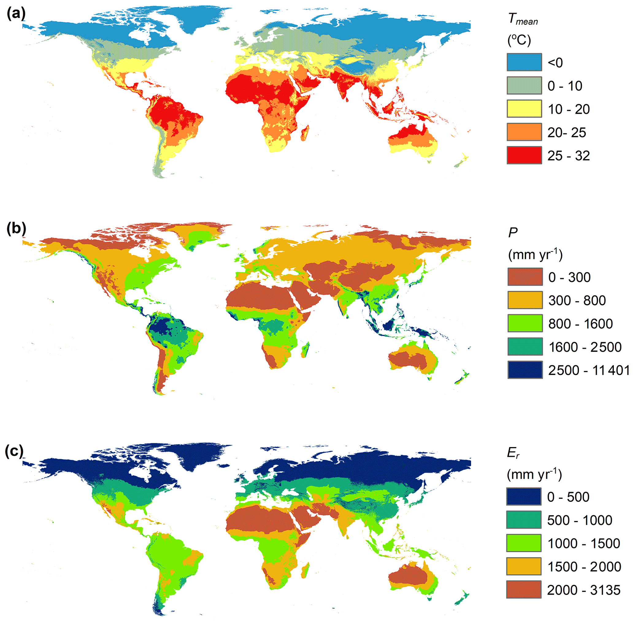
Figure 1(a) Mean annual temperature for the period (Hijmans et al., 2005), (b) mean annual precipitation for the period (Hijmans et al., 2005), and (c) mean annual reference evapotranspiration of ASCE-standardized method for short reference crop for the period (Aschonitis et al., 2017) of 1950–2000.
The derivation–calibration procedure was performed at a global scale using global gridded data from two databases. The first database of Hijmans et al. (2005) provides gridded data of mean monthly precipitation P and mean monthly temperature T of the period 1950–2000 (WorldClim version 1.2) at 30 arcsec spatial resolution (∼ 1 × 1 km at the Equator) (Fig. 1a, b). The second database is of Aschonitis et al. (2017) and provides gridded data of mean monthly reference evapotranspiration Er of the period 1950–2000 at five different resolutions (30 arcsec, 2.5 arcmin, 5 arcmin, 10 arcmin, and 0.5∘) (Fig. 1c). The method used for estimating Er is the ASCE-standardized method (formerly FAO-56 Penman–Monteith), which estimates reference evapotranspiration for short, clipped grass (Allen et al., 2005). The database of Er (Aschonitis et al., 2017) was built using the temperature from the first database of Hijmans et al. (2005) at 30 arcsec resolution, and for this reason the two gridded databases are compatible.
The validation procedure was performed using raw data of stations from three different databases. The first database is the CIMIS database (California Irrigation Management System – CIMIS, https://cimis.water.ca.gov/stations.aspx, last access: 1 October 2020), which includes stations from California, USA, and it was selected because it provides a dense and descriptive network of stations for a specific region that combines semiarid/temperate coastal, plain, and mountain environments. In total 60 stations (Fig. 2a) were used from the CIMIS database that have at least 15 years of observations, with a significant part of their observations after 2000. The second database is the AGBM database (Australian Government – Bureau of Meteorology, http://www.bom.gov.au, last access: 1 June 2020). This database includes many stations from Australia and was selected because the station's network covers a large territory with a large variety of climate classes from desert to tropical climate. The selection of stations was performed in order to cover all the possible existing Köppen–Geiger climatic types (Peel et al., 2007) and altitude ranges that exist in the Australian territory. In total 80 stations were used (Fig. 2b) that have at least 15 years of observations, with a significant part of their observations after 2000. The third database is the ECAD database (European Climate Assessment & Database, https://www.ecad.eu, last access: 1 February 2020). This database is a network that contains more than 20 000 stations throughout Europe and provides daily observations of climatological parameters. In this study, a final number of 385 stations (Fig. 2c) was selected from this database because they contained complete data of precipitation, temperature, solar radiation, relative humidity, and wind speed for a period of at least 20 years with a significant part of their observations after 2000. Some additional stations from the three databases (CIMIS, AGBM, ECAD), which do not have at least 15 years of observations, were selected due to their special Köppen–Geiger climate class or the high altitude of their location. The total final number of stations used in the study from the three databases is 525, and their full description is given in Table S1 of the Supplement.
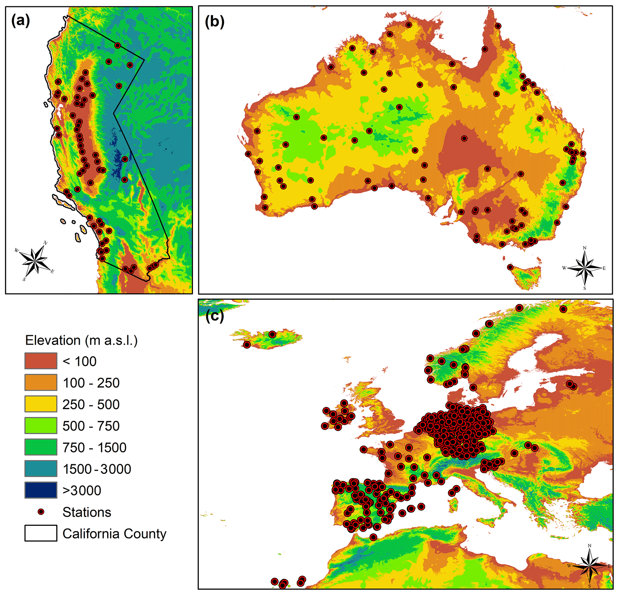
Figure 2(a) The 60 stations in California from the CIMIS database, (b) 80 stations in Australia from the AGBM database, and (c) 385 stations in Europe from the ECAD database.
2.2 Derivation and validation of Thornthwaite correction coefficients for short reference crop based on ASCE-standardized method
The monthly potential evapotranspiration Ep using the Thornthwaite (1948) method after its adjustment for variable daylight and month lengths (Willmott et al., 1985) is estimated as follows.
where , if X≤0 then X=0.00001
Here Ep is the mean monthly potential evapotranspiration or potential evapotranspiration of month i (millimeters per month), Tmean,i is the mean monthly temperature (∘C), n is the number of days in the month, N is the mean length of daylight of the days of the month (hours), J is the annual heat index, ji is the monthly heat index, α is the function of the annual heat index, and dj is the Julian day.
The benchmark method that was used for developing correction coefficients for the temperature-based method of Thornthwaite Ep is the ASCE-standardized method (formerly FAO-56 Penman–Monteith), which estimates reference evapotranspiration from short, clipped grass as follows (Allen et al., 2005):
where Er is the reference evapotranspiration (mm d−1), Δ is the slope of the saturation vapor pressure–temperature curve (kPa ∘C−1), Rn is the net radiation at the crop surface (MJ m−2 d−1), G is the soil heat flux density at the soil surface (MJ m−2 d−1), γ is the psychrometric constant (kPa ∘C−1), u2 is the wind speed at 2 m above the soil surface (m s−1), es is the saturation vapor pressure (kPa), ea is the actual vapor pressure (kPa),Tmean is the mean daily air temperature (∘C), and Cn and Cd are constants, which vary according to the time step and the reference crop type and describe the bulk surface resistance and aerodynamic roughness. Equation (3) can be applied for two types of reference crop (i.e., short and tall). The short reference crop (ASCE-short) corresponds to clipped grass of 12 cm height and surface resistance of 70 s m−1, where the constants Cn and Cd have the values 900 and 0.34, respectively (Allen et al., 2005). The use of Eq. (3) in daily or monthly steps for short reference crop is equivalent to the FAO-56 method (Allen et al., 1998), and this is how it is used in this study.
The derivation of a correction coefficient for Eq. (1) using as a benchmark the values of Eq. (3) is performed based on the same procedure proposed by Aschonitis et al. (2017) that has been used before for developing partially weighted annual correction coefficients for Priestley–Taylor and Hargreaves–Samani evapotranspiration methods. The procedure starts with the derivation of the monthly coefficient cth,i for each month i based on Eq. (5). Applying this procedure, 12 values of monthly cth,i are produced. The 12 monthly cth coefficients are then used to build mean annual coefficients. As was mentioned in Aschonitis et al. (2017), the efficiency of mean annual correction coefficients is mainly associated with their ability to better describe the larger values of the dependent variable (i.e., the values of Er during summer/hot months) and not the smaller values during cold periods when the absolute errors () are smaller. For this reason, weighted annual averages based on the monthly cth,i coefficients are estimated considering the participation weight of each month in the annual Er. Moreover, under cold conditions, the monthly coefficients cth,i may present unrealistic values that significantly affect the weighted averages. To solve this problem, threshold values for the monthly Ep,i and Er,i were used before the inclusion of their cth,i in the weighted average estimations. Preliminary analysis showed that when the mean monthly Ep,i and/or Er,i values are below ∼ 45 mm per month (∼ 1.5 mm d−1), then unrealistic mean monthly cth,i values occur (as unrealistic values are considered those that are at least 1 order of magnitude larger or smaller than 1). Taking into account the above, the following procedure was performed in order to obtain a partially weighted average based on monthly cth,i values after excluding those months with Er and/or Ep≤45 mm per month as follows.
Here cth,i is the monthly correction coefficient, Fr,i is the filter function for the reference method (ASCE) with values of 0 or 1, Fm,i is the filter function for the understudy model (Thornthwaite formula) with values of 0 or 1, is the adjusted monthly value of Er,i from the ASCE-short method that becomes 0 when Fr,i or Fm,i is 0, is the annual sum of the monthly adjusted values, Cth is the annual partially weighted average (p.w.a.) of the monthly cth,i coefficients for short reference crop, and i is the index of each month. Considering the above, the final corrected Thornthwaite formula for monthly calculations is given by the following equation:
where Eps,i is the corrected temperature-based short reference crop evapotranspiration (millimeters per month) of month i.
The above procedure was followed to calibrate the annual partially weighted average Cth (Eq. 10) for every location on the globe based on mean monthly Er and Ep of 1950–2000 using
-
the gridded mean monthly temperature data of Hijmans et al. (2005) that were further used to estimate the original mean monthly gridded Thornthwaite Ep (Eq. 1) for the period 1950–2000 (in the form of 12 raster datasets of Ep for each month) and
-
the respective mean monthly grids of Er based on ASCE-standardized for short reference crop (Eq. 1) from Aschonitis et al. (2017) (in the form of 12 raster datasets of Er for each month).
The validation procedure with the data of the 525 stations was performed by comparing the mean monthly and the mean annual benchmark values of Er (Eq. 4) versus the original Ep (Eq. 1) and versus the corrected Eps Thornthwaite formula (Eq. 11) considering the annual partially weighted average coefficients Cth at the location of each station. The validation was performed separately for each database of stations (ECAD, AGBM, CIMIS) but also all together using the following five statistical criteria.
Here MAE is the mean absolute error, ME the mean error, RMSE the root-mean-square error, RSqr the coefficient of determination, d the index of agreement, O the observed or benchmark value (i.e., Er), S the value simulated by the model (i.e., Ep or Eps), N the number of observations, and i the subscript referring to each observation. The value of perfect fit is 0 for the criteria MAE, ME, and RMSE while 1 is a perfect fit for the criteria RSqr and d. The values of the MAE, ME, and RMSE criteria have the same units as the observed and simulated data while RSqr and d are unitless.
2.3 Evaluating the use of correction coefficients in aridity indices based on station data
The role of the new corrected formula of Thornthwaite (Eq. 11) as an internal parameter of aridity indices was also evaluated against the original method (Eq. 1). For this purpose, the AIUNEP (UNEP, 1997) and AITH (Thornthwaite, 1948) aridity indices were used. The difference between the two indices is that AIUNEP does not consider seasonality. The two indices estimated based on Er (Eq. 4) were used as the benchmark in order to compare the respective indices calculated with the original Thornthwaite Ep (Eq. 1) and the corrected Eps (Eq. 11) using the 525 stations' data. The evaluation was performed
-
by comparing the estimated aridity classes of 525 stations produced by the benchmark AIUNEP and AITH values using Er versus the classes of the two indices using Ep and Eps, respectively, and
-
by comparing the respective values of the indices using 1 : 1 plots and the statistical metrics of Eqs. (12)–(16).
The AIUNEP aridity index is the simpler method for hydroclimatic analysis, and it is given by the following equation:
where Py is mean annual precipitation (mm yr−1) and Ey is mean annual potential evapotranspiration (mm yr−1). The values of Eq. (16) are classified according to the following (UNEP, 1997; Cherlet et al., 2018):
-
AIUNEP < 0.05 → hyper-arid
-
0.03 ≤ AIUNEP < 0.2 → arid
-
0.2 ≤ AIUNEP < 0.5 → semiarid
-
0.5 ≤ AIUNEP < 0.65 → dry subhumid
-
0.65 < AIUNEP → humid
The classes for AIUNEP > 0.65 are usually given as one humid class. The UNEP index does not consider the effect of seasonal variation in precipitation and potential evapotranspiration.
The AITH aridity index is calculated as follows:
and
where Pi and Ei are the monthly precipitation and potential evapotranspiration of month i, respectively. S (mm yr−1) considers only the positive values of (Pi−Ei) > 0, while (Pi−Ei) < 0 values are set to 0. In the case of D (mm yr−1), only the positive values of (Ei−Pi) > 0 are considered while for (Ei−Pi) < 0 they are set to 0. The various climatic types according to AITH values are the following.
-
−60 > AITH → hyper-arid (HE)
-
−60 ≤ AITH < −40 → arid (E)
-
−40 ≤ AITH < −20 → semiarid (D)
-
−20 ≤ AITH < 0 → dry sub-humid (C1)
-
0 ≤ AITH < 20 → moist sub-humid (C2)
-
20 ≤ AITH < 40 → low humid (B1)
-
40 ≤ AITH < 60 → moderate humid (B2)
-
60 ≤ AITH < 80 → highly humid (B3)
-
80 ≤ AITH < 100 → very humid (B4)
-
100 ≤ AITH → hyper-humid (A)
3.1 Derivation and validation of the Cth correction coefficients
The global map of the Cth correction coefficient was developed following the procedure described in Sect. 2.2, and it is given in Fig. 3. The validation of the derived Cth coefficients was performed for each one of the three datasets of stations (California, CIMIS; Australia, AGBM; Europe, ECAD), separately, by comparing the performance of mean monthly values (Fig. S1a–f, Supplement) and the performance of mean annual values (Fig. S2a–f, Supplement) of Ep (Eq. 1) and Eps (Eq. 11) versus the benchmark values of Er (Eq. 4). The statistical criteria (Eqs. 12–16) for both monthly and annual comparisons for each one of the three datasets of stations are given in Table 1. The respective monthly and annual comparisons after merging all the stations from the three datasets are also presented in Fig. 4a–d. From the results shown in Figs. S1, S2, and 4 and Table 1, a much better performance of Eps compared to the original Thornthwaite formula Ep is observed in all cases, providing not only better monthly but also better annual reference evapotranspiration estimations that approximate the values of ASCE for short reference grass.
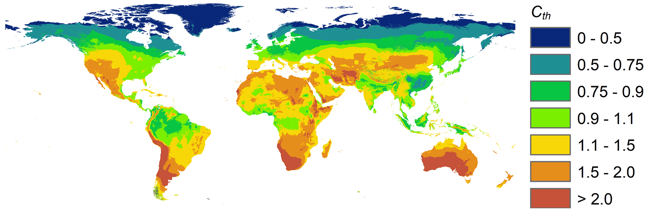
Figure 3Global map of the annual partially weighted average Cth coefficients.
Table 1Statistical metrics (Eqs. 12–16) for the comparisons between Ep vs. Er and Eps vs. Er for CIMIS (California), AGBM (Australia), and ECAD (Europe) stations (the unit for MAE, ME, and RMSE is millimeters per month).
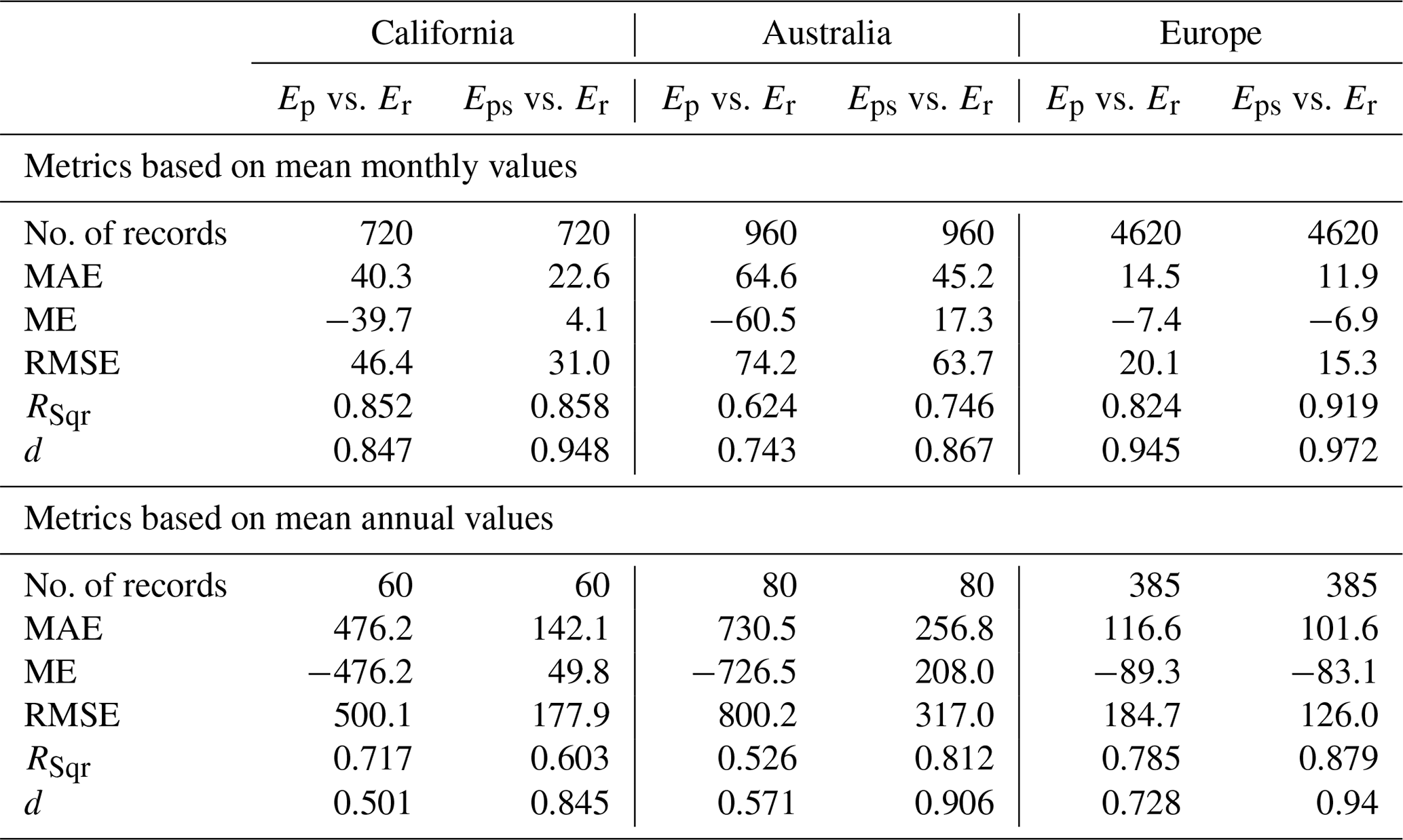
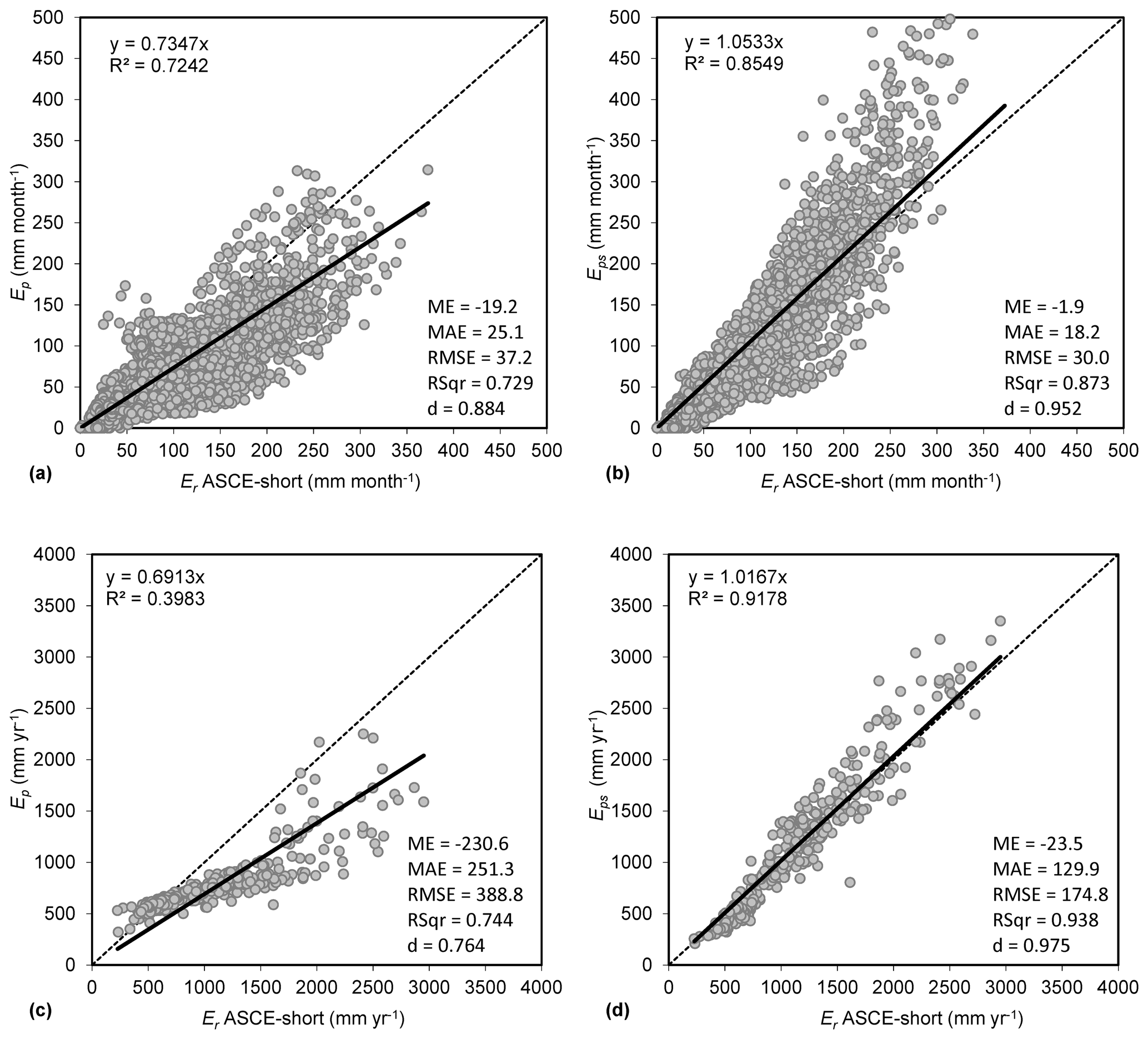
Figure 4(a) The 1 : 1 plots of mean monthly Ep versus mean monthly Er, (b) mean monthly Eps versus mean monthly Er, (c) mean annual Ep versus annual monthly Er, and (d) mean annual Eps versus annual monthly Er, using the data of all 525 stations from the three databases CIMIS, AGBM, and ECAD.
3.2 Evaluating the use of Cth coefficient in AIUNEP and AITH aridity indices
The use of Cth coefficients in AIUNEP and AITH aridity indices was also evaluated based on the raw data of all 525 stations (California, CIMIS; Australia, AGBM; Europe, ECAD).
The aridity classes of 525 stations given by the benchmark AIUNEP using Er were 76 % identical with the classes of the AIUNEP using Ep and 93 % identical with the classes of the AIUNEP using Eps. Similarly, the aridity classes of 525 stations given by the benchmark AITH using Er were 52 % identical with the classes of the AITH using Ep and 58 % identical with the classes of the AITH using Eps. Eps showed better performance compared to Ep at correctly identifying the aridity classes in both indices. The lower percentages of success in the case of AITH for both Ep and Eps are due to the double number of classes of AITH in comparison to AIUNEP. Merging the B and A classes of AITH to one humid class, as in the case of AIUNEP, the successful identical codes with Er are raised to 63 % for Ep and 76 % for Eps.
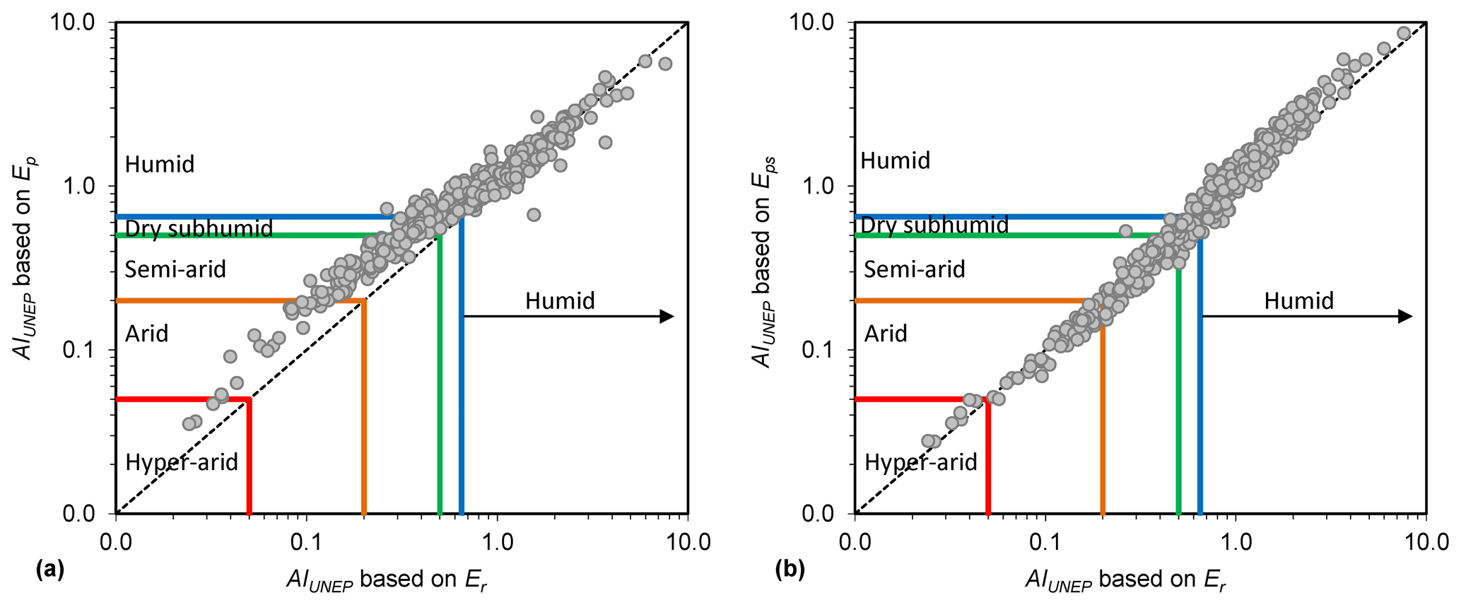
Figure 5(a) The 1 : 1 log-log plots of AIUNEP using mean monthly Ep versus AIUNEP using mean monthly Er and (b) AIUNEP using mean monthly Eps versus mean monthly Er using the data of all 525 stations from the three databases CIMIS, AGBM, and ECAD.
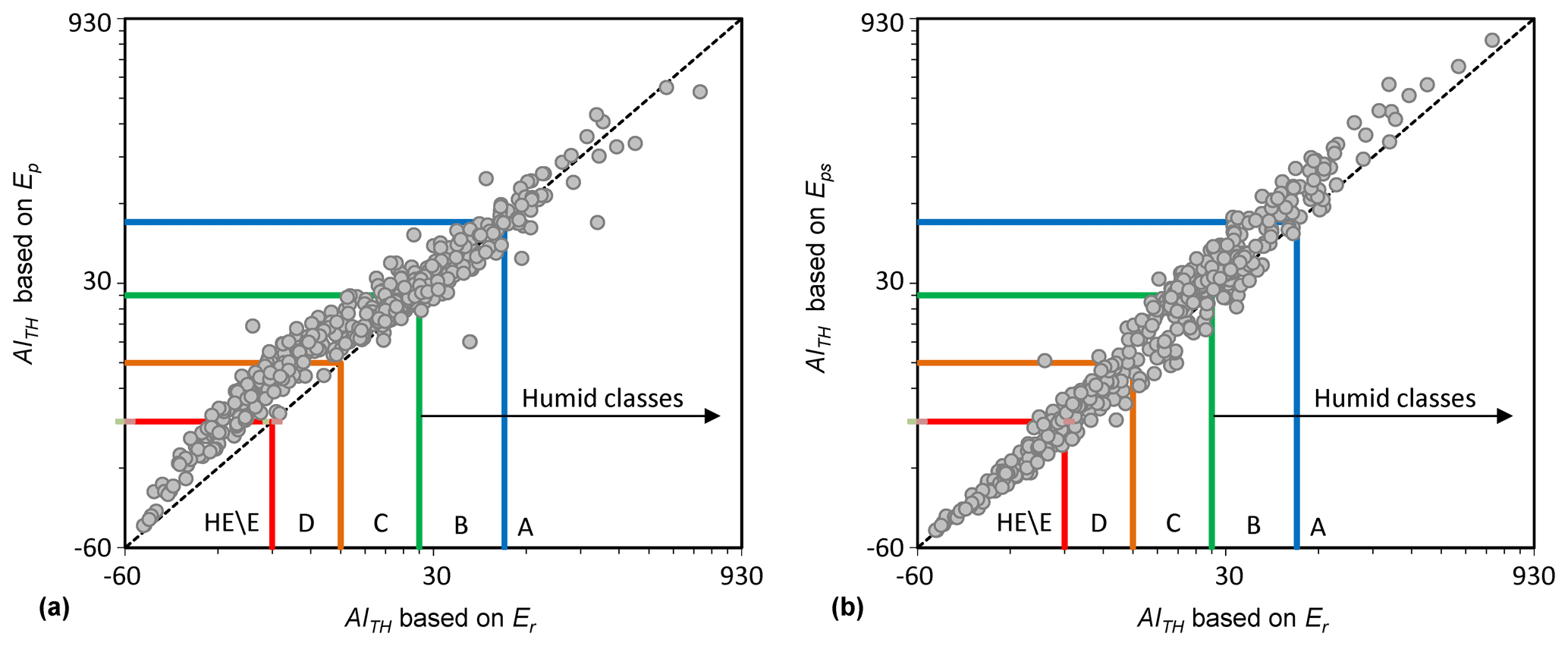
Figure 6(a) The 1 : 1 log-log plots of AITH using mean monthly Ep versus AITH using mean monthly Er and (b) AITH using mean monthly Eps versus mean monthly AITH using the data of all 525 stations from the three databases CIMIS, AGBM, and ECAD.
Table 2Statistical metrics (Eqs. 12–16) for the comparisons between Ep vs. Er and Eps vs. Er when they are applied in the (a) AIUNEP and (b) AITH aridity indices by dividing the 525 stations into two groups based on non-humid or humid classes of each index (MAE, ME, and RMSE are unitless as the indices).
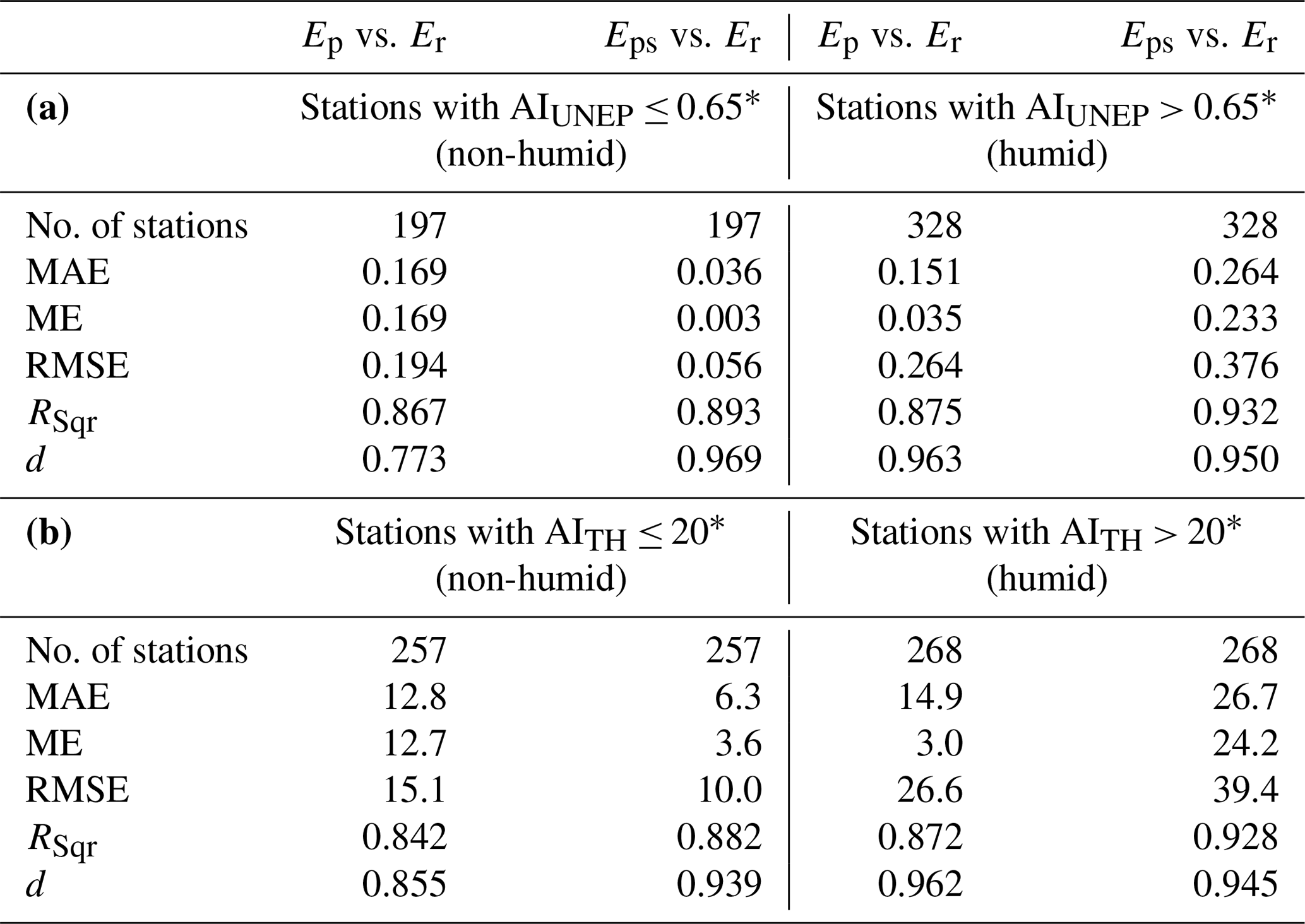
∗ Estimated by the benchmark Er.
The 1 : 1 log-log plots of AIUNEP using Er versus the AIUNEP using Ep and Eps are given in Fig. 5a, b, respectively, while the same comparisons using AITH are given in Fig. 6a, b. The visual inspection of Figs. 5 and 6 clearly shows that Eps outperforms Ep in the range of non-humid classes of both AIUNEP and AITH. To highlight this result, the statistical metrics (Eqs. 12–16) were estimated after splitting the stations into two groups (non-humid and humid) based on the respective thresholds of humid classes of each index calculated using Er (Table 2). Table 2 verifies the better performance of Eps compared to Ep in both AIUNEP and AITH aridity indices for the non-humid classes.
On the other hand, the statistics showed that Ep showed better performance in both AIUNEP and AITH aridity indices for their respective humid classes. This result is of less importance since Eps showed better performance compared to Ep at correctly identifying the aridity classes in both indices based on all stations despite the fact that the stations belonging to humid classes were more in both indices (Table 2). Moreover, in the case of AIUNEP, there is only one humid class (AIUNEP > 0.65), and thus there is no point in comparing the performance of Ep and Eps from a statistical point of view since their values will always lead to the same classification code/characterization (i.e., humid). In the case of AITH > 20, the same justification of AIUNEP could be used since the detailed division of five humid classes (B1, B2, B3, B4, A) provided by AITH was proposed for the alternative use of the index as a “humidity index” (Thornthwaite, 1948).
4.1 Validity of the derived Cth for periods beyond the calibration period
The derivation of local Cth coefficients at a global scale was performed using the mean monthly grid datasets of 1950–2000 assuming stationary climate conditions, while the validation was performed using stations' raw data from California and Australia that are expanded up to 2016 and stations' raw data from Europe that are expanded up to 2020 (Table S1). The reasons for choosing the specific grid datasets for the derivation of Cth coefficients are the following.
-
They are in the form of high-resolution grids (30 arcsec, ∼ 1 km at Equator), which have been developed using interpolation techniques that include the effects of latitude, longitude, and elevation. These grids allow us to derive more representative Cth values for every position even when weather stations do not locally exist.
-
They cover a large period of time (i.e., 1950–2000), so they can provide more representative mean annual p.w.a. Cth values. The upper threshold of the year 2000 of these grids also allows the validation dataset of stations to be more valid since the larger part of their data is after 2000, and this reduces the possibility of having been used in grids' development.
On the other hand, several works have shown climate differences after 2000 (Hansen et al., 2010; McVicar et al., 2012a, b; Wild et al., 2013; Willet et al., 2014; Sun et al., 2017). Such changes could possibly affect the validity of Cth coefficients and the final estimated values of Er for periods beyond 2000. For this reason, the Cth values and the mean monthly Er values of the grids of Aschonitis et al. (2017) of the period 1950–2000 were extracted from the positions of all 525 stations and compared with the respective values of computed Er and Cth using stations' raw data, which go beyond 2000. The results of this comparison are given in Fig. S3a, b (Supplement) and clearly show that the gridded Er data and Cth of 1950–2000 do not show serious deviations from their respective values for periods beyond 2000, allowing their safe use. Moreover, the fact that the original Thornthwaite (1948) formula was built before 1950 using data from the eastern and central USA and that the Cth values of the specific territories range between 0.9–1.1 for 1950–2000 (Fig. 3), it is not only a verification of the Cth derivation methodology but also an additional indication of a generalized temporal stability of Cth.
In the case of Fig. S3b, there is a distinctly deviated Cth pair of values from the 1 : 1 line (point indicated by a red arrow), which is associated with a specific station belonging to the Centro de Investigación Atmosférica de Izaña. This station is an exceptional case since it is at the top of a mountain at 2371 m a.s.l. on Tenerife (Canary Islands). The derived Cth of this station from the grid of the period 1950–2000 is almost half (Cth value equal to 1.37) of the one estimated using stations' raw data (Cth value equal to 2.44). This large difference is not the result of climate difference before and after 2000, but it is fully justified by the fact that the Cth value of the grid corresponds to an area of ∼ 1 km2 while the specific position of the station is unique, which can be described as the most extreme position within this pixel. There are also three stations on Tenerife in lowland areas where the derived Cth values of 1950–2000 are in agreement with those estimated by the stations' raw data.
4.2 Scale and other effects on the accuracy of the derived Cth
The case of Izana station on Tenerife was the perfect example for triggering further investigation for the possible effects of scale in similar environments with extremely variable topography. Investigating the individual stations with the larger percentage of deviation of Eps from Er, a relative systematic deviation was observed at some stations of the CIMIS (California) database, which are concentrated at the coastline between Los Angeles and San Diego. The specific region is a narrow (∼ 20–30 km), highly urbanized coastal zone of ∼ 200 km, which is enclosed between the coastline and a hilly/mountainous zone. At the specific stations, the average of Cth values of the period 1950–2000 from the position of these stations was 1.85, while the average of Cth values using their raw data was estimated at 1.46. Apart from the large topographic variation, another reason for the Cth differences at these stations could be the bias that has been removed by clearing extreme flagged wind values in the data of the CIMIS database, which are probably associated with frequent extreme events in this region (extreme winds, droughts including wildfires, and heavy precipitation). This could justify the fact that the gridded Cth values of 1950–2000 at the positions of the stations are greater than the Cth values estimated by their raw data from CIMIS after removing flagged extreme values.
An additional analysis based only on the stations of California was made to show that a wider regional mean value of Cth coefficient could also be an additional option, especially when the whole territory is described by local Cth coefficients that are only > 1 or only < 1 (in California all local Cth coefficients are > 1). For this analysis, the average value of Cth=1.66 was estimated based on the values of local Cth coefficients of 1950–2000 from the locations of all stations of CIMIS (California). The mean monthly and mean annual Eps values of these stations were computed using Cth=1.66 for all of them and compared with the respective Er values estimated with stations' raw data (Fig. S4a, b, Supplement). The results of Fig. S4a, b showed that even a regional average of Cth values for California can lead to better results of Eps compared to Ep as it was given for monthly and annual estimations in Figs. S1a and S2a, respectively.
4.3 Justifications about the methodology for deriving annual Cth correction coefficients based on partially weighted averages
The initial trials to derive annual correction coefficients Cth of this study were made using the average value of the 12 monthly cth,i values of each i month. This procedure led to unreasonably high values due to the extreme high values during winter. An example of this problem based on the gridded data used in the calibration–derivation procedure is given in Fig. S5a (Supplement), which corresponds to a position close to Lake Garda in Italy (45.45∘ N, 10.124∘ E). According to Fig. S5a, the annual average of monthly cth,i values for this location is equal to 2.4 due to the extremely high values during winter and especially during January. Using the 2.4 value as the annual correction coefficient, the Eps,i value of July becomes equal to 338 mm, which is 203 mm larger than the respective Er,i value of July (Fig. S5a). The specific procedure for deriving annual Cth coefficients was rejected due to this problem. A second approach was to use the 12 pairs of monthly Er and Ep for each position on the grid in order to perform regression analysis based on the form without intercept based on the form of . An example of the specific procedure is given in Fig. S5b using the data of Fig. S5a, where the annual Cth value was found equal to 0.98. The specific procedure provides annual Cth values, which are always closer to the monthly coefficients of the warmer months since optimization algorithms try to minimize the total error, which mainly originates in the months that show larger evapotranspiration values. Despite the fact that the specific procedure pays less attention to the monthly cth,i values of colder months, it was considered acceptable since most of the hydroclimatic applications require higher accuracy for the larger evapotranspiration values rather than the lower ones.
A similar approach with the one of Fig. S5b was performed by Cristea et al. (2013) for deriving annual correction coefficients for the Priestley–Taylor method for 106 stations across the contiguous USA. The correction coefficients were estimated for each station by minimizing the sum of the squared residuals between Priestley–Taylor and the benchmark FAO-56, considering data only for the period April–September (warmer semester). The obtained optimized values of the correction coefficients for each station were then interpolated to produce a map of the Priestley–Taylor correction coefficients. For our study, the specific procedure was found to be extremely demanding in computing requirements since it was impossible to be performed pixel by pixel (777.6 million pixels) with a conventional computer unit for the whole globe using as input 24 rasters of extremely high resolution (∼ 1 km) with a total size of ∼ 70 GB. In order to solve this problem, the method using partially weighted averages (Eqs. 5–10) developed by Aschonitis et al. (2017) was used, which provides similar results to the regression analysis of but allows us to perform calculations step by step with a conventional computer unit in the GIS environment using large gridded databases. For the data of Fig. S5a, the partially weighted average method provided a Cth value equal to 0.99, which is almost equal to 0.98 of Fig. S5b. The method of partially weighted averages is also extremely efficient since it is not restricted only to the warmer semester or to any other predefined period like the case of Cristea et al. (2013) since it controls all months one by one using the threshold of 45 mm per month, which is more appropriate for global applications and especially for applications of high-resolution data, giving the appropriate weight to the months with significant values of evapotranspiration.
The threshold of 45 mm per month was derived empirically after analyzing many datasets using monthly and mean monthly data. In the case of monthly data, a representative example is given in Fig. S6a, b (Supplement) using the monthly data of Embrun station in France (44.57∘ N, 6.50∘ E) 1980–2020. Figure S6a shows the box–whisker plots of monthly Er,i values of the station, while Fig. S6b shows the respective box–whisker plots of monthly cth,i values. The maximum cth,i values of December, January, and February are outside the plot of Fig. S6b, with values of 30.1, 129.4, and 210.1, respectively. Figure S6a, b show that the monthly cth,i values of months with Er,i < 45 mm per month are extremely unstable, and their mean monthly value, even if it seems normal, cannot guarantee its safe use. In the case of mean monthly data, a representative example is given in Fig. 7, where the 6300 mean monthly cth,i values derived by the raw data of the 525 stations were plotted against their respective mean monthly Er values using a 2D density scatter plot. Figure 7 shows that the mean monthly cth,i values of the stations start to exhibit extremely high dispersion below the threshold of 45 mm per month, with values reaching 1 order of magnitude larger than unity. In the case where there is a location where all months show Er or Ep values below 45 mm per month, it is suggested to either use the non-zero Cth value of the closer location in the map of Fig. 3 or directly use the original Thornthwaite formula without correction.
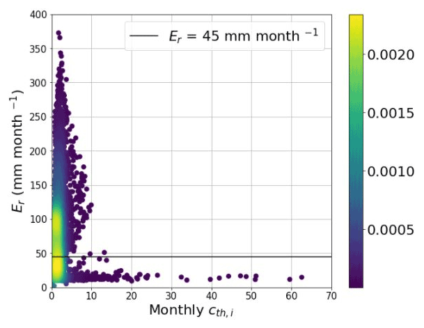
Figure 7The 2D scatter density plot between the 6300 mean monthly cth,i values versus the respective mean monthly Er values derived by the raw data of the 525 stations ( or non-defined due to Er and/or Ep=0 not being included in the graph).
The produced global database of local Cth coefficients of this study has been archived in PANGAEA and can be assessed using the following link: https://doi.org/10.1594/PANGAEA.932638 (Aschonitis et al., 2021). The database is provided at five different resolutions (30 arcsec, 2.5 arcmin, 5 arcmin, 10 arcmin, 0.5∘). The coarser resolutions are provided in order to cover the observed resolution range in the initial climatic data used for developing the published Er gridded data by Aschonitis et al. (2017) (e.g., the temperature data of Hijmans et al., 2005, were provided at 30 arcsec resolution, while the solar radiation, humidity, and wind speed data of Sheffield et al., 2006, were provided at 0.5∘ resolution and rescaled to 30 arcsec using bilinear interpolation). The data of different resolutions can be used as a tool to assess uncertainties associated with temperature variation effects within different resolution pixels or to estimate average values of the coefficients for larger territories, which have problems at coarse resolutions (e.g., coastlines or islands that do not exist in 0.5∘ resolution), taking into account the concept and concerns of Daly (2006).
A global database of local correction coefficients for improving the performance of the monthly temperature-based Thornthwaite potential evapotranspiration method was built using gridded data covering the period 1950–2000. The method for developing the correction coefficients was based on partially weighted averages of their respective mean monthly values estimated as the monthly ratios between the benchmark ASCE-standardized Er method (formerly FAO-56) versus the original Thornthwaite Ep. The correction coefficients were produced as partially weighted averages of monthly ratios by setting the ratios' weight according to the monthly Er magnitude and by excluding colder months because the ratio becomes highly unstable for low temperatures. The correction coefficients were validated using raw data from 525 stations of California, Australia, and Europe that include independent data beyond 2000 up to 2020. The results showed that the correction coefficients significantly improved the monthly and annual results of the original Thornthwaite method Ep. The use of Ep with or without correction coefficients was also evaluated through their use in the aridity indices of Thornthwaite and UNEP versus the respective indices estimated based on the benchmark ASCE-standardized Er. The results showed again that the correction coefficients significantly improved the performance of the indices compared to the original Thornthwaite method, especially in non-humid environments. The global database of local correction coefficients supports applications of reference evapotranspiration and aridity index assessment with minimum data requirements (i.e., mean temperature) for locations where climate data are limited. Uncertainties in the values of correction coefficients were observed in regions of high topographic variability, and a recommendation for such cases is the use of a regional average of correction coefficients or the use of local Cth values based on the available coarser resolutions provided in the database. The methods and results presented in this study and the observed uncertainties can be used as a base for future works focusing on (a) the validation of the correction coefficients for other places in the world, (b) comparison with other models of low data requirements, and (c) use of the p.w.a. method for recalibrating correction coefficients using station or climate models' data of recent periods.
The supplement related to this article is available online at: https://doi.org/10.5194/essd-14-163-2022-supplement.
The idea behind the work was conceived by VA, the data processing was carried out by VA and DT, and quality control, visualization, and writing were completed by VA, DT, MCG, and MCtV.
The contact author has declared that neither they nor their co-authors have any competing interests.
Publisher’s note: Copernicus Publications remains neutral with regard to jurisdictional claims in published maps and institutional affiliations.
This paper was edited by David Carlson and reviewed by one anonymous referee.
Allen, R., Pereira, L., Raes, D., and Smith, M.: Crop evapotranspiration – Guidelines for computing crop water requirements-FAO Irrigation and drainage paper 56, FAO – Food and Agriculture Organization of the United Nations, Rome, Italy, available at: http://www.fao.org/3/X0490E/x0490e00.htm#Contents (last access: 1 April 2020), 1998.
Allen, R. G., Walter, I. A., Elliott, R., Howell, T., Itenfisu, D., Jensen, M., and Snyder, R. L.: The ASCE Standardized Reference Evapotranspiration Equation, American Society of Civil Engineers, Idaho, https://doi.org/10.1061/9780784408056, 2005.
Almorox, J., Quej, V. H., and Martí, P.: Global performance ranking of temperature-based approaches for evapotranspiration estimation considering Köppen climate classes, J. Hydrol., 528, 514–522, https://doi.org/10.1016/j.jhydrol.2015.06.057, 2015.
Asadi Zarch, M. A., Sivakumar, B., and Sharma, A.: Assessment of global aridity change, J. Hydrol., 520, 300–313, https://doi.org/10.1016/j.jhydrol.2014.11.033, 2015.
Aschonitis, V. G., Papamichail, D., Demertzi, K., Colombani, N., Mastrocicco, M., Ghirardini, A., Castaldelli, G., and Fano, E.-A.: High-resolution global grids of revised Priestley–Taylor and Hargreaves–Samani coefficients for assessing ASCE-standardized reference crop evapotranspiration and solar radiation, Earth Syst. Sci. Data, 9, 615–638, https://doi.org/10.5194/essd-9-615-2017, 2017.
Aschonitis, V. G., Touloumidis, D., ten Veldhuis, M.-C., and Coenders-Gerrits, M.: Correcting Thornthwaite evapotranspiration formula using a global grid of local coefficients to support temperature-based estimations of reference evapotranspiration and aridity indices, PANGAEA [data set], https://doi.org/10.1594/PANGAEA.932638, 2021.
Baier, W. and Robertson, G. W.: Estimation of latent evaporation from simple weather observations, Can. J. Plant Sci., 45, 276–284, https://doi.org/10.4141/cjps65-051, 1965.
Bakundukize, C., Van Camp, M., and Walraevens, K.: Estimation of Groundwater Recharge in Bugesera Region (Burundi) using Soil Moisture Budget Approach, Geol. Belgica, 14, 85–102, 2011.
Bautista, F., Bautista, D., and Delgado-Carranza, C.: Calibration of the equations of Hargreaves and Thornthwaite to estimate the potential evapotranspiration in semi–arid and subhumid tropical climates for regional applications, Atmosfera, 22, 331–348, 2009.
Beguería, S., Vicente-Serrano, S. M., Reig, F., and Latorre, B.: Standardized precipitation evapotranspiration index (SPEI) revisited: Parameter fitting, evapotranspiration models, tools, datasets and drought monitoring, Int. J. Climatol., 34, 3001–3023, https://doi.org/10.1002/joc.3887, 2014.
Brinckmann, S., Krähenmann, S., and Bissolli, P.: High-resolution daily gridded data sets of air temperature and wind speed for Europe, Earth Syst. Sci. Data, 8, 491–516, https://doi.org/10.5194/essd-8-491-2016, 2016.
Camargo, A. P., Marin, F. R., Sentelhas, P. C., and Picini, A. G.: Adjust of the Thornthwaite's method to estimate the potential evapotranspiration for arid and superhumid climates, based on daily temperature amplitude, Rev. Bras. Agrometeorol., 7, 251–257, 1999.
Castañeda, L. and Rao, P.: Comparison of methods for estimating reference evapotranspiration in Southern California, J. Environ. Hydrol., 13, 1–10, 2005.
Cherlet, M., Hutchinson, C., Reynolds, J., Hill, J., Sommer, S., and Von Maltitz, G.: World atlas of desertification rethinking land degradation and sustainable land management, Publication Office of the European Union, Luxembourg, https://doi.org/10.2760/9205, 2018.
Cristea, N., Kampf, S., Burges, S., and Asce, F.: Revised Coefficients for Priestley-Taylor and Makkink-Hansen Equations for Estimating Daily Reference Evapotranspiration, J. Hydrol. Eng., 18, 1289–1300, https://doi.org/10.1061/(ASCE)HE.1943-5584.0000679, 2013.
Dai, A.: Increasing drought under global warming in observations and models, Nat. Clim. Chang., 3, 52–58, https://doi.org/10.1038/nclimate1633, 2013.
Daly, C.: Guidelines for assessing the suitability of spatial climate data sets, Int. J. Climatol., 26, 707–721, https://doi.org/10.1002/joc.1322, 2006.
Droogers, P. and Allen, R. G.: Estimating Reference Evapotranspiration Under Inaccurate Data Conditions, Irrig. Drain. Syst., 16, 33–45, https://doi.org/10.1023/A:1015508322413, 2002.
Hamon, W. R.: Estimating Potential Evapotranspiration, J. Hydraul. Div., 87, 107–120, 1961.
Hamon, W. R.: Computation of direct runoff amounts from storm rainfall, Int. Assoc. Sci. Hydrol. Publ., 63, 52–62, 1963.
Hansen, J., Ruedy, R., Sato, M., and Lo, K.: Global Surface Temperature Change, Rev. Geophys., 48, 1–29, https://doi.org/10.1029/2010RG000345, 2010.
Hargreaves, G. H. and Samani, Z. A.: Estimating potential evapotranspiration, J. Irrig. Drain. Eng., 108, 225–230, 1982.
Harris, I., Jones, P. D., Osborn, T. J., and Lister, D. H.: Updated high-resolution grids of monthly climatic observations – The CRU TS3.10 dataset, Int. J. Climatol., 34, 623–642, https://doi.org/10.1002/joc.3711, 2014.
Hijmans, R. J., Cameron, S. E., Parra, J. L., Jones, P. G., and Jarvis, A.: Very high resolution interpolated climate surfaces for global land areas, Int. J. Climatol., 25, 1965–1978, https://doi.org/10.1002/joc.1276, 2005.
Holdridge, L. R.: Life zone ecology, Tropical Science Center, Costa Rica, available at: http://reddcr.go.cr/sites/default/files/centro-de-documentacion/holdridge_1966_-_life_zone_ecology.pdf (last access: 1 March 2021), 1967.
Jain, P. K. and Sinai, G.: Evapotranspiration Model for Semiarid Regions, J. Irrig. Drain. Eng., 111, 369–379, https://doi.org/10.1061/(ASCE)0733-9437(1985)111:4(369), 1985.
Liu, X., Li, C., Zhao, T., and Han, L.: Future changes of global potential evapotranspiration simulated from CMIP5 to CMIP6 models, Atmosph. Ocean. Sci. Lett., 13, 568–575, https://doi.org/10.1080/16742834.2020.1824983, 2020.
Malmström, V. H.: A New Approach To The Classification Of Climate, J. Geog., 68, 351–357, https://doi.org/10.1080/00221346908981131, 1969.
McCloud, D. E.: Water requirements of field crops in Florida as influenced by climate, Proc. Soil Crop Sci. Soc. Florida, 15, 165–172, 1955.
McMahon, T. A., Peel, M. C., Lowe, L., Srikanthan, R., and McVicar, T. R.: Estimating actual, potential, reference crop and pan evaporation using standard meteorological data: a pragmatic synthesis, Hydrol. Earth Syst. Sci., 17, 1331–1363, https://doi.org/10.5194/hess-17-1331-2013, 2013.
McVicar, T. R., Roderick, M. L., Donohue, R. J., and Van Niel, T. G.: Less bluster ahead? ecohydrological implications of global trends of terrestrial near-surface wind speeds, Ecohydrology, 5, 381–388, https://doi.org/10.1002/eco.1298, 2012a.
McVicar, T. R., Roderick, M. L., Donohue, R. J., Li, L. T., Van Niel, T. G., Thomas, A., Grieser, J., Jhajharia, D., Himri, Y., Mahowald, N. M., Mescherskaya, A. V, Kruger, A. C., Rehman, S., and Dinpashoh, Y.: Global review and synthesis of trends in observed terrestrial near-surface wind speeds: Implications for evaporation, J. Hydrol., 416–417, 182–205, https://doi.org/10.1016/j.jhydrol.2011.10.024, 2012b.
Osborn, T. J. and Jones, P. D.: The CRUTEM4 land-surface air temperature data set: construction, previous versions and dissemination via Google Earth, Earth Syst. Sci. Data, 6, 61–68, https://doi.org/10.5194/essd-6-61-2014, 2014.
Oudin, L., Hervieu, F., Michel, C., Perrin, C., Andréassian, A., Anctil, F., and Loumagne, C.: Which potential evapotranspiration input for a lumped rainfall–runoff model?: Part 2 – Towards a simple and efficient potential evapotranspiration model for rainfall–runoff modelling, J. Hydrol., 303, 290–306, https://doi.org/10.1016/j.jhydrol.2004.08.026, 2005.
Palmer, W.: Meteorological Drought, Research paper no. 45, U.S. Department of Commerce Weather Bureau, Washington, D.C., available at: https://www.ncdc.noaa.gov/temp-and-precip/drought/docs/palmer.pdf (last access: 1 March 2021), 1965.
Peel, M. C., Finlayson, B. L., and McMahon, T. A.: Updated world map of the Köppen-Geiger climate classification, Hydrol. Earth Syst. Sci., 11, 1633–1644, https://doi.org/10.5194/hess-11-1633-2007, 2007.
Penman, H. L.: Natural evaporation from open water, hare soil and grass, Proc. R. Soc. Lond. A. Math. Phys. Sci., 193, 120–145, https://doi.org/10.1098/rspa.1948.0037, 1948.
Pereira, A. R. and Pruitt, W. O.: Adaptation of the Thornthwaite scheme for estimating daily reference evapotranspiration, Agric. Water Manag., 66, 251–257, https://doi.org/10.1016/j.agwat.2003.11.003, 2004.
Proutsos, N. D., Tsiros, I. X., Nastos, P., and Tsaousidis, A.: A note on some uncertainties associated with Thornthwaite's aridity index introduced by using different potential evapotranspiration methods, Atmos. Res., 260, 105727, https://doi.org/10.1016/j.atmosres.2021.105727, 2021.
Quej, V. H., Almorox, J., Arnaldo, J. A., and Moratiel, R.: Evaluation of Temperature-Based Methods for the Estimation of Reference Evapotranspiration in the Yucatán Peninsula, Mexico, J. Hydrol. Eng., 24, 05018029, https://doi.org/10.1061/(ASCE)HE.1943-5584.0001747, 2019.
Sanikhani, H., Kisi, O., Maroufpoor, E., and Yaseen, Z. M.: Temperature-based modeling of reference evapotranspiration using several artificial intelligence models: application of different modeling scenarios, Theor. Appl. Climatol., 135, 449–462, https://doi.org/10.1007/s00704-018-2390-z, 2019.
Sheffield, J., Goteti, G., and Wood, E. F.: Development of a 50-Year High-Resolution Global Dataset of Meteorological Forcings for Land Surface Modeling, J. Climate, 19, 3088–3111, https://doi.org/10.1175/JCLI3790.1, 2006.
Sheffield, J., Wood, E. F., and Roderick, M. L.: Little change in global drought over the past 60 years, Nature, 491, 435–438, https://doi.org/10.1038/nature11575, 2012.
Shuttleworth, W. J.: Evaporation, Handbook of Hydrology, 41, 505–572, https://doi.org/10.1021/ie50529a034, 1993.
Sun, X., Ren, G., Xu, W., Li, Q., and Ren, Y.: Global land-surface air temperature change based on the new CMA GLSAT data set, Sci. Bull., 62, 236–238, https://doi.org/10.1016/j.scib.2017.01.017, 2017.
Thornthwaite, C.: An Approach toward a Rational Classification of Climate, Geogr. Rev., 38, 55–94, https://doi.org/10.2307/210739, 1948.
Trajkovic, S.: Temperature-Based Approaches for Estimating Reference Evapotranspiration, J. Irrig. Drain. Eng., 131, 316–323, https://doi.org/10.1061/(asce)0733-9437(2005)131:4(316), 2005.
Trajkovic, S.: Hargreaves versus Penman-Monteith under Humid Conditions, J. Irrig. Drain. Eng., 133, 38–42, https://doi.org/10.1061/(asce)0733-9437(2007)133:1(38), 2007.
Trajkovic, S. and Kolakovic, S.: Estimating reference evapotranspiration using limited weather data, J. Irrig. Drain. Eng., 135, 443–449, https://doi.org/10.1061/(ASCE)IR.1943-4774.0000094, 2009a.
Trajkovic, S. and Kolakovic, S.: Evaluation of reference evapotranspiration equations under humid conditions, Water Resour. Manag., 23, 3057–3067, https://doi.org/10.1007/s11269-009-9423-4, 2009b.
Trajkovic, S., Gocic, M., Pongracz, R., and Bartholy, J.: Adjustment of Thornthwaite equation for estimating evapotranspiration in Vojvodina, Theor. Appl. Climatol., 138, 1231–1240, https://doi.org/10.1007/s00704-019-02873-1, 2019.
Trajkovic, S., Gocic, M., Pongracz, R., Bartholy, J., and Milanovic, M.: Assessment of Reference Evapotranspiration by Regionally Calibrated Temperature-Based Equations, KSCE J. Civ. Eng., 24, 1020–1027, https://doi.org/10.1007/s12205-020-1698-2, 2020.
Trenberth, K. E., Dai, A., van der Schrier, G., Jones, P. D., Barichivich, J., Briffa, K. R., and Sheffield, J.: Global warming and changes in drought, Nat. Clim. Chang., 4, 17–22, https://doi.org/10.1038/nclimate2067, 2014.
UNEP: World atlas of desertification, United nations environment programme, 2nd edn., London, available at: https://wedocs.unep.org/20.500.11822/30300 (last access: 1 March 2021), 1997.
Van Der Schrier, G., Jones, P. D., and Briffa, K. R.: The sensitivity of the PDSI to the Thornthwaite and Penman-Monteith parameterizations for potential evapotranspiration, J. Geophys. Res.-Atmos., 116, D03106, https://doi.org/10.1029/2010JD015001, 2011.
Van Der Schrier, G., Barichivich, J., Briffa, K. R., and Jones, P. D.: A scPDSI-based global data set of dry and wet spells for 1901–2009, J. Geophys. Res.-Atmos., 118, 4025–4048, https://doi.org/10.1002/jgrd.50355, 2013.
Wang, K. and Dickinson, R. E.: A review of global terrestrial evapotranspiration: Observation, modeling, climatology, and climatic variability, Rev. Geophys., 50, RG2005, https://doi.org/10.1029/2011RG000373, 2012.
Weiß, M. and Menzel, L.: A global comparison of four potential evapotranspiration equations and their relevance to stream flow modelling in semi-arid environments, Adv. Geosci., 18, 15–23, https://doi.org/10.5194/adgeo-18-15-2008, 2008.
Wild, M., Folini, D., Schär, C., Loeb, N., Dutton, E. G., and König-Langlo, G.: The global energy balance from a surface perspective, Clim. Dynam., 40, 3107–3134, https://doi.org/10.1007/s00382-012-1569-8, 2013.
Willett, K. M., Dunn, R. J. H., Thorne, P. W., Bell, S., de Podesta, M., Parker, D. E., Jones, P. D., and Williams Jr., C. N.: HadISDH land surface multi-variable humidity and temperature record for climate monitoring, Clim. Past, 10, 1983–2006, https://doi.org/10.5194/cp-10-1983-2014, 2014.
Willmott, C. J., Rowe, C. M., and Mintz, Y.: Climatology of the terrestrial seasonal water cycle, J. Climatol., 5, 589–606, https://doi.org/10.1002/joc.3370050602, 1985.
Yang, Q., Ma, Z., Zheng, Z., and Duan, Y.: Sensitivity of potential evapotranspiration estimation to the Thornthwaite and Penman–Monteith methods in the study of global drylands, Adv. Atmos. Sci., 34, 1381–1394, https://doi.org/10.1007/s00376-017-6313-1, 2017.
Yuan, S. and Quiring, S. M.: Drought in the U.S. Great Plains (1980–2012): A sensitivity study using different methods for estimating potential evapotranspiration in the Palmer Drought Severity Index, J. Geophys. Res.-Atmos., 119, 10996–11010, https://doi.org/10.1002/2014jd021970, 2014.
Zhang, J., Sun, F., Xu, J., Yaning, C., Sang, Y.-F., and Liu, C.: Dependence of trends in and sensitivity of drought over China (1961–2013) on potential evaporation model, Geophys. Res. Lett., 43, 206–213, https://doi.org/10.1002/2015GL067473, 2015.
Zhang, Y., Liu, S., Wei, X., Liu, J., and Zhang, G.: Potential Impact of Afforestation on Water Yield in the Sub-Alpine Region of Southwestern China, JAWRA J. Am. Water Resour. Assoc., 44, 1144–1153, https://doi.org/10.1111/j.1752-1688.2008.00239.x, 2008.
Zomer, R. J., Trabucco, A., Bossio, D. A., van Straaten, O., and Verchot, L. V.: Climate change mitigation: A spatial analysis of global land suitability for clean development mechanism afforestation and reforestation. Agr. Ecosyst. Environ, 126, 67–80, https://doi.org/10.1016/j.agee.2008.01.014 2008.