the Creative Commons Attribution 4.0 License.
the Creative Commons Attribution 4.0 License.
 | 28 Mar 2022
High-resolution spatial-distribution maps of road transport exhaust emissions in Chile, 1990–2020
Mauricio Osses
Néstor Rojas
Cecilia Ibarra
Víctor Valdebenito
Ignacio Laengle
Nicolás Pantoja
Darío Osses
Kevin Basoa
Sebastián Tolvett
Nicolás Huneeus
Laura Gallardo
Benjamín Gómez
This description paper presents a detailed and consistent estimate and analysis of exhaust pollutant emissions generated by Chile's road transport activity for the period 1990–2020. The complete database for the period 1990–2020 is available at the following DOI: https://doi.org/10.17632/z69m8xm843.2 (Osses et al., 2021). Emissions are provided at a high spatial resolution (0.01∘ × 0.01∘) over continental Chile from 18.5 to 53.2∘ S, including local pollutants (CO; volatile organic compounds, VOCs; NOx; PM2.5), black carbon (BC) and greenhouse gases (CO2, CH4). The methodology considers 70 vehicle types, based on 10 vehicle categories, subdivided into 2 fuel types and 7 emission standards. Vehicle activity was calculated based on official databases of vehicle records and vehicle flow counts. Fuel consumption was calculated based on vehicle activity and contrasted with fuel sales to calibrate the initial dataset. Emission factors come mainly from the Computer programme to calculate emissions from road transport version 5 (COPERT 5), adapted to local conditions in the 15 political regions of Chile, based on emission standards and fuel quality. While vehicle fleet grew 5-fold between 1990 and 2020, CO2 emissions have followed this trend at a lower rate, and emissions of air local pollutants have decreased due to stricter abatement technologies, better fuel quality and enforcement of emission standards. In other words, there has been decoupling between fleet growth and emissions' rate of change. Results were contrasted with global datasets (EDGAR, CAMS, CEDS), showing similarities in CO2 estimations and striking differences in PM, BC and CO; in the case of NOx and CH4 there is coincidence only until 2008. In all cases of divergent results, global datasets estimate higher emissions.
- Article
(4565 KB) - Full-text XML
- BibTeX
- EndNote


Building and updating emission inventories provide key information for designing and evaluating public policies concerning topics relevant to city inhabitants' quality of life, the environment and mitigation of climate change (Kuenen et al., 2014; Creutzig et al., 2015). In international and national experiences, the construction of reliable emission inventories for road transport has been a bottleneck in mapping the emissions in cities (Zheng et al., 2014). In general, these difficulties occur for two main reasons: the lack of disaggregated data at a level to construct detailed inventories and the many variables to consider when modelling emissions, increasing the uncertainty in the estimation of total emissions (Bond et al., 2004; Tolvett et al., 2016).
Latin America has an urbanization rate of more than 80 %, and cities suffer changes in local climate and air pollution, imposing big challenges to cope with (Henríquez and Romero, 2019; Hardoy and Romero-Lankao, 2011). Transport in cities is a major source of air pollution and emissions of greenhouse gases (GHGs) (Huneeus et al., 2020a). Reliable inventories are needed to assess policy measures for air quality and climate change. In the case of Santiago, Chile's capital, there are good examples of the use of local data to analyse the impact of emissions on air pollution (Mazzeo et al., 2018) and the health benefits of policy scenarios (Mena-Carrasco et al., 2012) and for retrospective evaluation of the evolution of mobility and air quality, relating them to policy measures (Gallardo et al., 2018).
Despite research results for specific data analysis, inventories for Chile have huge scope for improvement in terms of data accuracy and disaggregation. Better inventories are needed for decision-making related to cities' air quality and for climate change commitments. Barraza et al. (2017) estimated that motor vehicles were responsible for 37.3 % of PM2.5 in Santiago, which highlights the role played by mobile sources in large urban areas. The transport sector at large accounts for 25 % of 2018 CO2 estimates in Chile (MMA, 2021). Further, in 2016, a fraction of 7 % of total black carbon (BC) is linked to the on-road transportation sector (Gallardo et al., 2020). International inventories include data for Chile; for example, EDGAR V4.3.2 covers between 1970 and 2012 and later until 2015 (Crippa et al., 2019) and recently EDGAR V5.0 extended its range to 2018 (Crippa et al., 2020).
Chile has two separate inventories, one for GHGs and another for criteria pollutants of air quality. The GHG inventory follows the methodology established by the Intergovernmental Panel on Climate Change; it has been systematically kept since 2012, and it includes estimates starting in 1990 (MMA, 2021). This inventory is made in-house at the Ministry of the Environment in coordination with other sectorial ministries, which assures capacity building within the ministry. Although this dataset is well evaluated and consistent, the level of aggregation is national or at best at split into political regions. On the other hand, inventories for criteria pollutants are built in connection with the establishment of attainment plans and produced through external consultancies, which has resulted in a scattered picture regarding reference years, emission factors used and cities across continental Chile. These inventories only consider specific industrial complexes or urban areas and not rural areas or background conditions, which limits the scope of attainment plans as highlighted by Huneeus et al. (2020b).
The recent commitment made by Chile before the Paris Agreement and the United Nations Framework Convention on Climate Change (UNFCCC) considers achieving carbon neutrality regarding GHGs by 2050 and reducing black carbon emissions by at least 25 % by 2030 with respect to levels in 2016 (Gobierno de Chile, 2020). To accurately monitor progress with respect to BC emissions will require an improved spatial resolution and explicit monitoring of BC in PM2.5 (Gallardo et al., 2020). The same applies when considering health impacts linked to PM and BC (Burnett et al., 2018; Kirrane et al., 2019)
Chile has included short-lived climate pollutants (SLCPs) in its inventories since 2012, when the Ministry of the Environment joined the Climate and Clean Air Coalition (CCAC) and committed to reducing emissions of SLCPs. One of the actions taken was to identify the main sources of these pollutants, concluding that transport was a main emission sector and that black carbon concentrations were worryingly high (Jorquera et al., 2017). Data on black carbon emissions were recently updated and show the situation has not changed significantly (Gallardo et al., 2020). Black carbon (BC) is a pollutant with impact on human health and contributes to climate change on a global and local scale (Bond et al., 2013; Hadley and Kirchstetter, 2012; Ramanathan and Carmichael, 2008), hence motivating the inclusion of a goal for black carbon reduction in Chile's nationally determined contributions to the UNFCCC (Gobierno de Chile, 2020).
This description paper presents an extension and update of the data for the emission inventory for on-road transport in Chile, considering fuel consumption records, the vehicle fleet, stricter emission standard requirements and the inclusion of motorcycles as a vehicular category. This inventory is based on previous methodologies (MAPS Chile, 2013; Osses et al., 2014; Jorquera et al., 2017; Gallardo et al., 2020; Zheng et al., 2014). It incorporates the latest data available, with the purpose of calculating transport activity to obtain an updated estimate of transport emissions and offering high-resolution spatially distributed maps for Chile.
The paper is structured as follows: Sect. 2 describes the methodology; Sect. 3 presents the main results showing the evolution of vehicle technologies and their impact on emissions and regional differences; Sect. 4 makes a comparison of results with the EDGAR, CAMS and CEDS datasets for the period 1990 to 2015; Sect. 5 concludes.
The annual emission database provides estimates of exhaust emissions for on-road transport, i.e. vehicles travelling on public routes, nationwide, in urban and rural areas, for the years 1990 to 2020. It does not include rail, air and sea transport modes and off-road machinery. The calculation of emissions was based on estimations of the number of vehicles and their activity level by political region, which were used to calculate fuel consumption by vehicle category and, subsequently, exhaust emissions, as summarized in the methodological diagram (Fig. 1) and explained in this section. The resultant emission database was spatially distributed at 0.01×0.01∘ of latitude and longitude resolution.

2.1 Vehicle fleet composition
Vehicle fleet composition was based on official government data on the annual registration of in-use vehicles, i.e. the vehicles that pay their circulation permit each year after having been approved according to a periodic technical inspection. The National Institute of Statistics (INE, https://www.ine.cl/, last access: 23 November 2021) provides annual reports of the total number of vehicles with a circulation permit per political region. Vehicle categories reported are light passenger, commercial and taxi vehicles; 12 and 18 m buses; light-, medium- and heavy-duty trucks; and two-wheeled motorized vehicles. Since the emission factors and fuel consumption of the distinct types of vehicles are modelled using the Computer programme to calculate emissions from road transport (COPERT) version 5 coordinated by the European Environment Agency (EMISIA, https://www.emisia.com/utilities/copert, last access: 23 November 2021) (Ntziachristos et al., 2009), the equivalence between Chilean INE categories and COPERT is shown in Table 1.
Table 1Equivalence of European and Chilean main vehicle categories. HDT denotes heavy-duty truck.
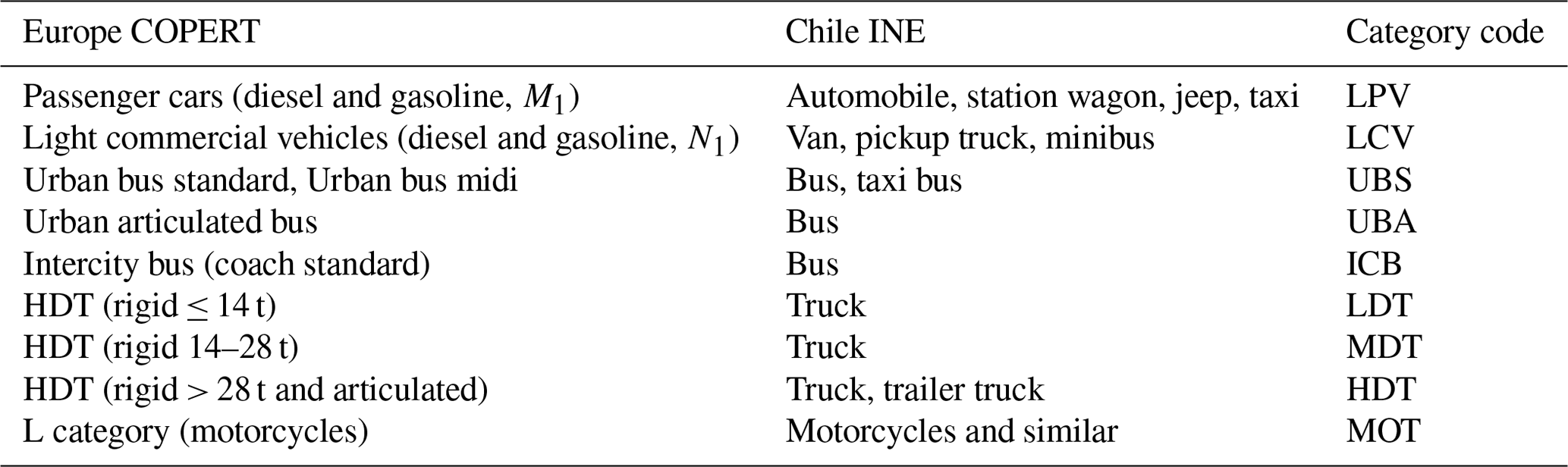
Each of these categories was subdivided to distinguish the type of fuel used (gasoline or diesel), using the most recent information from the Ministry of Transport and Telecommunications (MTT) and the Transport Secretariat (Osses et al., 2014), and the technology used, based on the emission standard in its European equivalent (Euro standard). To model the vehicle technology distribution, we used information given in the supreme decrees of MTT and the Ministry of the Environment (MMA), corresponding to the enforcement of emission technology standards for new vehicles entering the national fleet (all vehicles are imported), for the distinct vehicular categories distinguishing between regions.
Table 2Introduction of emission standards for vehicle categories in Chile.
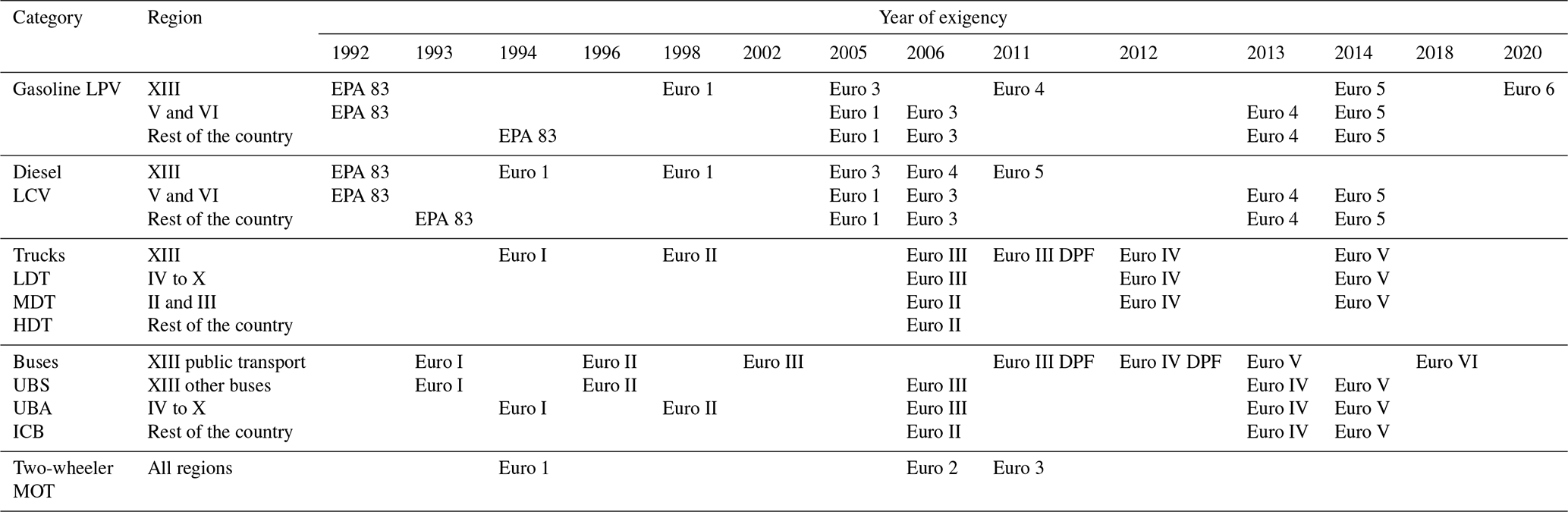
Roman number notation applies to heavy-duty vehicles, and Arabic numbers apply to light commercial and passenger vehicles. EPA 83: the Environmental Protection Agency's 1983 emission standards. DPF: diesel particulate filter.
Information in Table 1 is based on the following government decrees: DS 82/93MTT, DS 54/94MTT, DS 55/94MTT, DS 130/2002MMT and DS 4/2012MMA, available at https://www.bcn.cl/leychile/ (last access: 24 November 2021).
The combination of categories, fuels and emission standards generates a total of 70 types of vehicles for the emission analysis, distributed over political regions and distinguishing between urban and interurban activity. The distribution of vehicles into urban and interurban activity per region was based on a proportional regional distribution according to Osses et al. (2010).
2.2 Calculation of vehicle activity and fuel consumption
The activity level is expressed as VKT (vehicle kilometres travelled) calculated as the sum of the vehicles in each type per kilometre driven (Eq. 1).
where is the number of vehicles of type i in region j and road class k (urban or interurban) and KM is the kilometres travelled per year by vehicles type i, in region j and road class k.
The kilometres travelled by each type of vehicle used in Eq. (1) are shown in Table 3. They correspond to estimations by Osses et al. (2014) and MAPS Chile (2013) for the first level of vehicle aggregation (main vehicle categories in Table 1).
Table 3Annual activity level per region and vehicle type (AL). Currently, there are 15 political regions in Chile numbered from I to XV, with XIII being the Santiago Metropolitan Region.
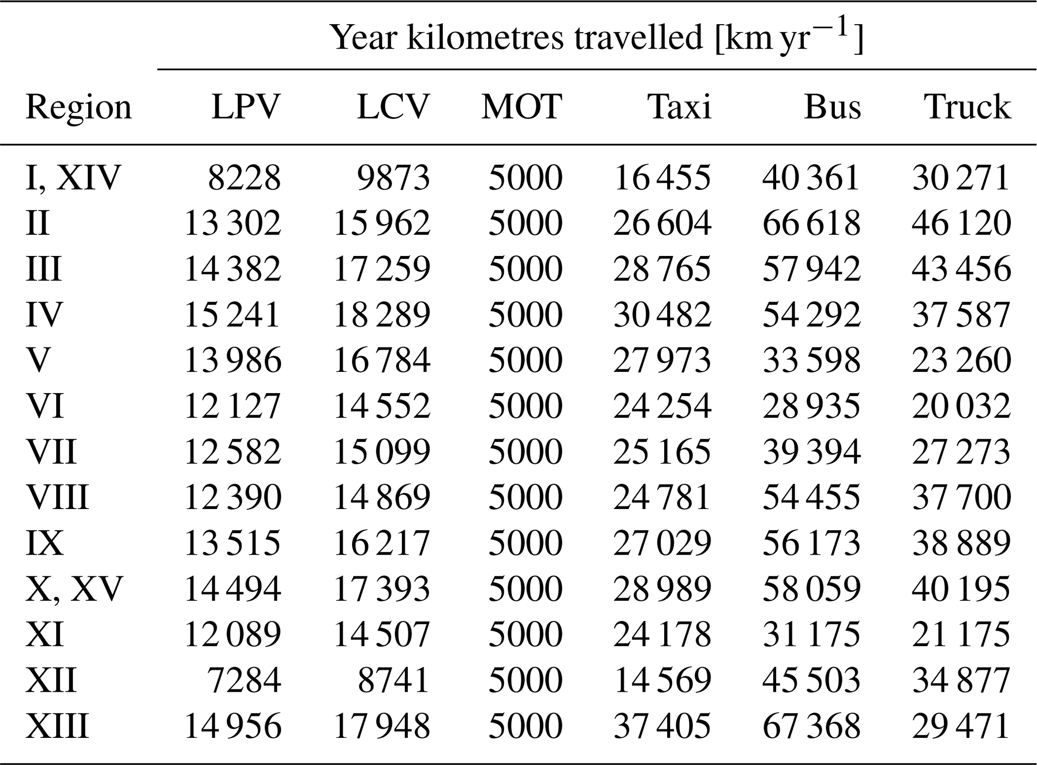
Source: authors' elaboration based on Osses et al. (2014).
Once the number of vehicles per region has been obtained, the total fuel consumption (TFC) for a given year is calculated as shown in Eq. (2):
where i is the region to which the vehicle belongs; j represents the vehicle type (passenger, commercial, bus, truck, motorcycle); k represents the share of the subcategory for the distinct vehicle types (the subcategories are for passenger and commercial vehicles diesel and gasoline; for buses rigid, articulated and intercity; and for trucks light-, medium- and heavy-duty); l represents the share of vehicles that drive in urban areas or on interurban roads; and m is the share of vehicles according to their emission control technology (pre-Euro I, Euro I–VI). The terms of Eq. (2) represent the following: AL is the annual activity level of the vehicle [km per year per vehicle], N is the total number of registered vehicles per year and per region where the sub-indices disaggregate this number into the subcategories mentioned, FC is the fuel consumption per vehicle [km L−1], X1 is the percentage of the distinct subcategories, X2 is the share of traffic counts depending on if the vehicle is driven in urban or rural areas, and X3 is the percentage of vehicles with distinct emission control technologies. Thus, Eq. (2) is used to calculate the total fuel consumption for each category presented as sub-indices.
TFC was compared to real fuel sales for each region. The Superintendency of Electricity and Fuels (SEC, http://www.sec.cl, last access: 23 November 2021) provides information on sales of diesel and gasoline for the transportation sector, by political region. The calculated TFC (see Eq. 2) was compared to the data given by SEC, and then a correction factor was applied to the total number of registered vehicles in each region to make these two fuel consumption values equal, correcting for those vehicles that are registered but do not contribute to actual driving activity. Thus, the number of active vehicles in a region was inferred and adjusted accordingly. A comparison between official figures of national fuel sales (SEC) and estimated TFC, for gasoline and diesel at a national level, is shown in Fig. 2.
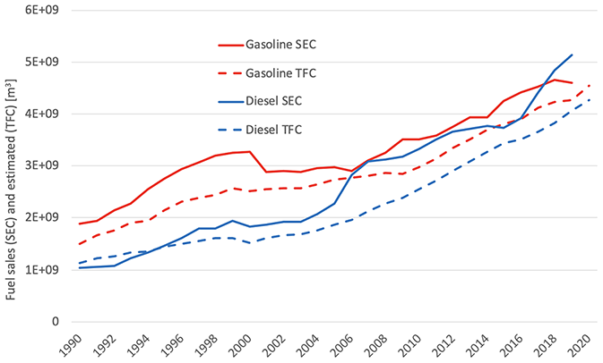
Figure 2National fuel sales and estimated total fuel consumption for gasoline and diesel in Chile.
In general, estimates of fuel consumption are lower than fuel sales, which means the number of registered vehicles generates lower activity than in reality or specific consumption factors for each vehicle technology are lower than the real driving conditions in Chile. These differences are addressed by increasing the number of vehicles according to their technology and matching official fuel sales figures.
2.3 Emission factors and annual emissions
The estimation of emissions considered that all vehicles that enter Chile are required to comply with the European Euro regulations or their US equivalent, according to the regulation requirements in Table 2 (Introduction of emission standards for vehicle categories in Chile). The assignment of emission factors for each of these vehicle types was carried out by applying COPERT 5 values (EEA, 2020), adapted to the Chilean fleet (Gómez, 2020). Total emissions are calculated multiplying VKT by an emission factor in grams per kilometre. The result is a regional emission database distinguishing between urban and interurban emissions, for CO, CO2, volatile organic compounds (VOCs), NOx, PM2.5, CH4 and BC.
With the calculated mobility demand, emissions of pollutants based on vehicle kilometres travelled by the different vehicular categories can be estimated through Eq. (3) (Zheng et al., 2014):
where the sub-index n represents the pollutant: CO2, CO, NOx, PM2.5, BC, and VOCs and CH4. EF is the emission factor for the pollutant n [g km−1] for each vehicle.
CO2, CO, NOx, PM2.5 and VOC emission factors are modelled using COPERT 5 methodology (Ntziachristos et al., 2009) based on the average speed in the driving cycles given by previous studies in all regions of Chile (Osses et al., 2014). The CH4 emission factors used are from previous reports (Ntziachristos et al., 2007; USEPA, 2018). However, COPERT 5 does not model black carbon emission factors due to the difficulty of the classification of this type of aerosol (Bond et al., 2013). Nonetheless, there have been studies to determine black carbon fractions in particulate matter, distinguishing between vehicle technology and fuel type, considering that elemental carbon and black carbon fractions are equivalent (Bond et al., 2004; Chow et al., 2010; Minjares et al., 2014; Ntziachristos et al., 2007). These fraction values can be used to obtain BC emission factors as follows:
where EFPM is the emission factor of the total particulate matter in the exhaust, F2.5 is the mass fraction of particles that have an aerodynamic diameter of 2.5 µm or less, and FBC is the fraction of black carbon in these particles. The mass fraction of fine particles used is 0.9 since in a generic and ideal particle distribution, between 80 % and 95 % of the total mass of the particles is concentrated in this range (Payri and Desantes, 2011). Table 4 shows the black carbon fractions used, distinguishing vehicle category, motorization and vehicle technology. Motorcycle BC emission factors used were taken from the literature (Cai et al., 2013).
Table 4 fractions for vehicle emission technologies in Chile.
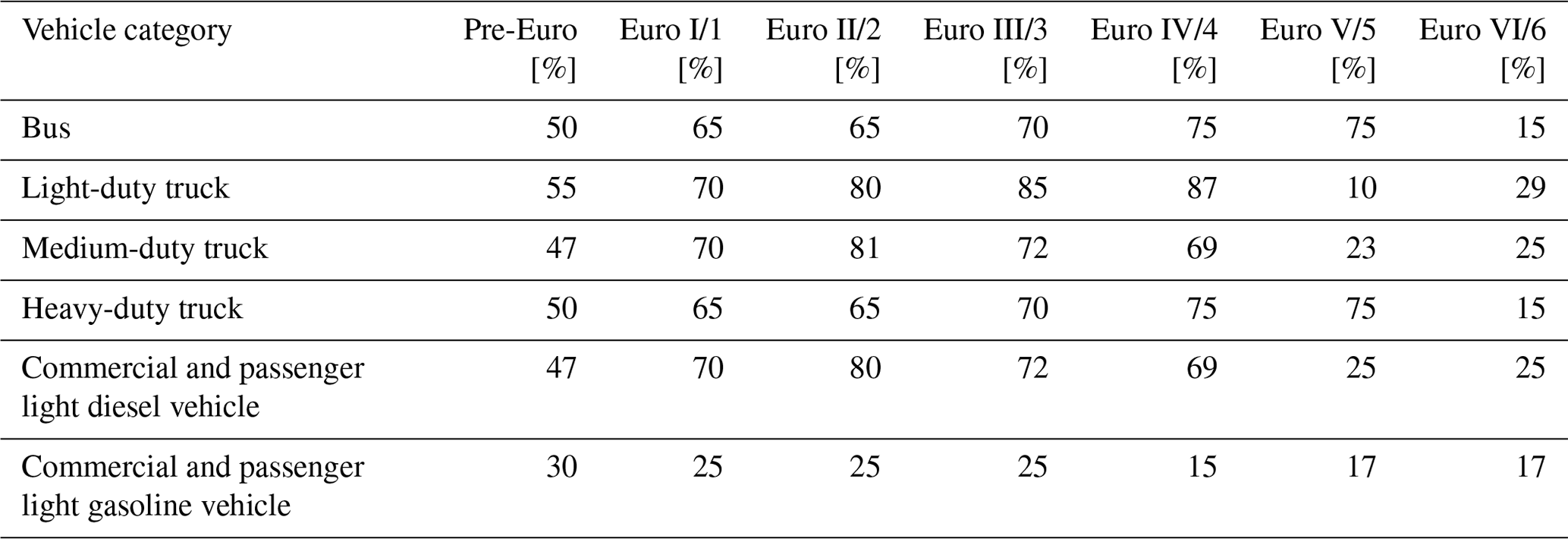
Roman number notation applies to heavy-duty vehicles, and Arabic numbers apply to light commercial and passenger vehicles.
COPERT 5 considers correction of emission factors by vehicle age for light vehicle categories Euro 3 and 4 and for VOCs, CO and NOx. These corrections were also applied.
2.4 Spatial disaggregation
The spatial distribution of transport emissions per political region consists of allocating gigagrams of emissions per year to each cell in a grid, with cells of 0.01×0.01∘ of latitude and longitude covering the 15 regions in the country. The regions correspond to the political administrative division of the territory. The distribution depends on the types of roads in each cell, the vehicle flow and the presence of urban populations.
The identification of roads in each cell was based on road network maps, available from the official road database for Chile and the official regional limits (BCN, 2020). The information on Chile's road network was complemented with data from OpenStreetMap (OSM, 2020). It covers a total of 77 800 km of rural and urban roads. Each road on the network was classified into a hierarchy comprising freeways, arterial roads, collectors and local roads. The estimation of vehicle flow on each type of road resulted from applying a road weight factor, based on toll barrier vehicle counts at interurban roads (MOP, 2020) and origin–destiny surveys on urban roads. Average weight factors are 54 % for freeways, 23 % on arterial roads, 16 % for collectors and 7 % on local roads. The road weight factors vary by region, urban and interurban area, and cities in a region and are provided by the Transport Secretariat, SECTRA (Osses et al., 2010).
Emissions were distributed over the road network using QGIS open-source software. Urban emissions were also distributed among the cities of each region according to their population (INE, 2017). QGIS allocates emissions to cells based on the types of roads, with their weight factor, and the presence of cities. Therefore, emissions for each cell depend on the roads and the presence of urban populations. The Transport Secretariat, SECTRA, provides the proportion of urban and interurban roads per region (Osses et al., 2010), and the urban areas of each region can be associated with cities with populations of over 5000 inhabitants. The number of kilometres in each cell is proportional to the annual emissions for each cell in the grid, and the sum of emissions in all cells coincides with the total emissions assigned to each region of the country.
3.1 Evolution of fuel quality, vehicle technology and emission factors
Based on the information given in Sect. 2.1 and 2.2, the number of vehicles and their technological evolution have been determined according to European emission standards (pre-Euro, Euro 1–6 for light-duty vehicles, Euro I–VI for trucks and buses). The enforcement of stricter emission standards across the country has been sustained by permanent national fuel quality improvements. The reduction in sulfur in fuels was progressive from 1990 to 2004, going from 5000 to 50 ppm of sulfur in diesel and from 1000 to 30 ppm in gasoline. In April 2001, the elimination of leaded gasoline was made effective, which allowed national enforcement of three-way catalytic converters, reducing the levels of CO, VOCs, NOx and also particulate matter from motor vehicles (Moreno et al., 2010). Since 2004 the levels of parts per million of sulfur in diesel and gasoline have been regulated by law for the whole country. The standard was fixed to 10 ppm for gasoline in the year 2010 (DS 66/2010MMA, available at https://www.bcn.cl/leychile/, last access: 20 November 2021.) and to 15 ppm for diesel in 2012 (DS 40.263/2012MMA). Currently, with the introduction of Euro 6/VI emission standards (DS 40/2019MMA), the maximum limit of sulfur in diesel is set at 10 ppm in the country. These policies, involving the introduction of better fuel quality and stricter emission standards (Table 2), are expected to keep decreasing the exhaust emissions of local pollutants from on-road transportation, even considering the permanent increase in mobility. The evolution of emission standards and number of vehicles for the whole country are shown in Figs. 3 and 4, adding up specific regional information from 1990 until 2020.
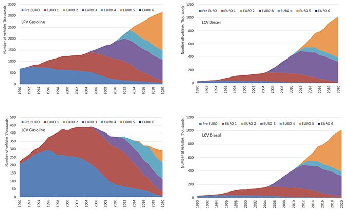
Figure 3Emission standards and vehicle fleet in Chile, 1990–2020, for light passenger vehicles (LPV) and light commercial vehicles (LCV), using gasoline and diesel respectively.
Figure 3 shows a continuous growth in light vehicles in Chile, except for the LCV-gasoline category, whose fall is offset by a strong increase in LCV-diesel vehicles. The total fleet of active light vehicles, both gasoline and diesel, grew from 968 000 to 5.1 million units between 1990 and 2020. The gradual disappearance of technologies prior to Euro requirements (pre-Euro) and Euro 1 standards is also observed, ending in 2020 with a fleet mixed between Euro 3 and Euro 5. By 2020 there were already a few Euro 6 vehicles, but they cannot be distinguished in the graphs.
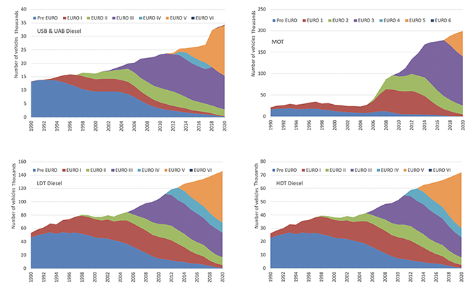
Figure 4Emission standards and vehicle fleet in Chile, 1990–2020, for urban standard buses (USB), urban articulated buses (UAB), two-wheelers (MOT), light-duty trucks (LDT) and heavy-duty trucks (HDT).
The vehicles in heavy diesel categories have similar behaviours. The number of heavy diesel vehicle units shows a sustained growth, going from 92 000 in 1990 to 250 000 in 2020, adding all types of buses and trucks in Chile. The introduction of standards has been gradual, with the disappearance of pre-Euro and Euro I vehicles in 2020, leaving a mixed fleet between Euro II and Euro V at the end of the analysis period. By 2020, the first low-emission buses for public transport were operating in the metropolitan region, with a total of 700 Euro VI units and 400 electric buses, which is almost imperceptible in the upper left graph of Fig. 4.
Two-wheel vehicles were not important in Chile until 2006, when they started to increase, all of them four-stroke. The fleet of 22 000 units in 1990 grew to 200 000 motorcycles in 2020, most of them complying with the Euro 4 standard. Growing urban congestion and the proliferation of home delivery services can explain this higher demand for motorcycles in Chile.
Knowing the different vehicle technologies in Chile and their equivalence with the European categories (Table 1), it is possible to obtain the emission factors from the values reported by the COPERT model (Ntziachristos et al., 2009). For doing this, different activity parameters are considered, where the most relevant are the average speed of displacement and load level. Table 6 shows the result of this assignment, considering urban speeds for light vehicles, buses and motorcycles and interurban speeds for trucks. The vehicle categories correspond to those indicated in Table 5.
Table 5Emission factors used for different compounds and vehicle categories in Chile, the numbers 0–6 indicate the corresponding Euro standards, and the letters G and D correspond to gasoline and diesel respectively.
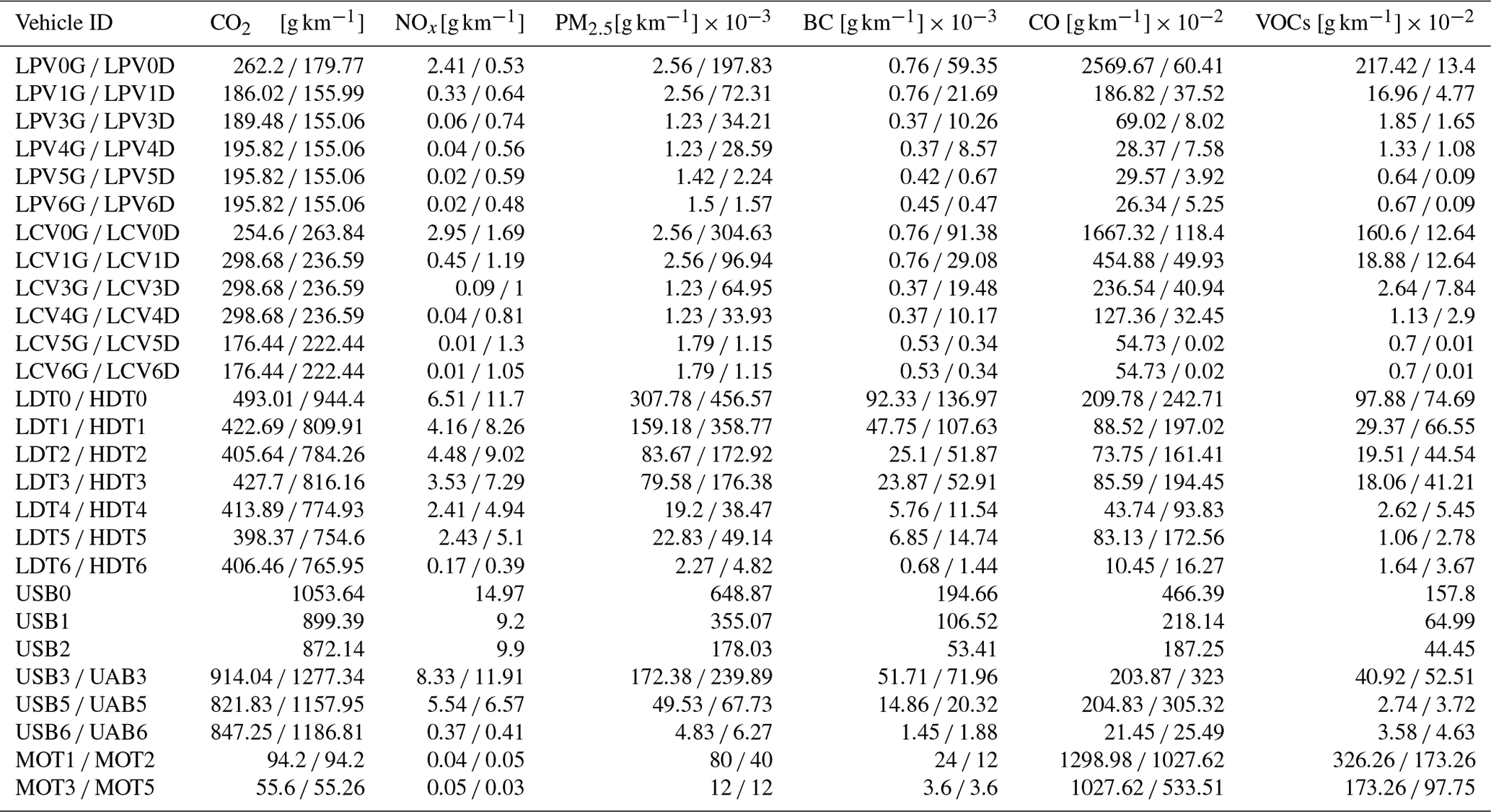
In total, 70 vehicle categories are generated, which are doubled to 140 types of emission when considering urban and interurban travelling speeds. All these emission types apply to the different pollutants, which are shown in Table 6. In general, all emission factors decrease as the level of the Euro standard is increased. CO2 emissions for gasoline vehicles are higher than for diesel vehicles, this compound being the one with the fewest reductions since all technologies burn fossil fuels. Diesel vehicles contribute most of the emissions of PM2.5, BC and NOx but with important reductions when going from Euro 4/IV to Euro 5/V or Euro 6/VI. It is interesting to note the high emission factors of PM2.5 and CO from motorcycles, especially considering their recent increase in the Chilean vehicle fleet.
3.2 Annual emission trends at a national level
Using the activity levels and emission factors previously described, total emissions are calculated by pollutant, vehicle type and country region. Table 6 shows a summary of the total annual emissions, with the variation percentages between 1990 and 2020. CO2 has an increase of 207.7 %, compared to 309 % in mobility growth (VKT) for the same period. CO2 official values for on-road transportation were reported by Chile from 2010 until 2018 (MMA, 2020), differing by ±1.4 % with values shown in Table 6 during those years.
Table 6Total annual exhaust emissions produced by on-road transportation in Chile, 1990–2020.
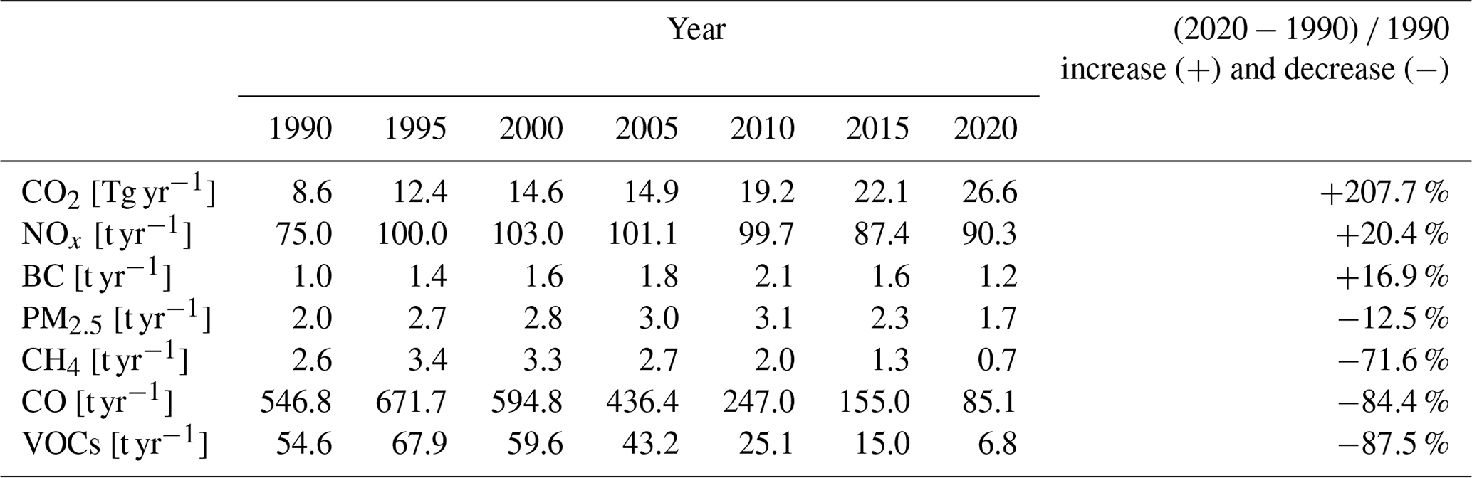
Unlike CO2, the rest of the local pollutants included in Table 6 are decoupled from the growth in mobility, reducing their contribution significantly thanks to technological improvements. NOx is the one with the least reduction compared with economic growth, with 20.4 % of emissions in 2020 compared to 1990. Emissions of PM2.5 and BC go up for the first 20 years of analysis, starting to decrease after 2010, when the reduction ratio of PM2.5 is greater than BC. CO and VOCs, mainly associated with gasoline engines, show significant reductions, mainly due to the massive incorporation of three-way catalytic converters required for vehicles complying with Euro standards.
Table 7Total annual exhaust emissions by vehicle type in Chile, 1990–2020.
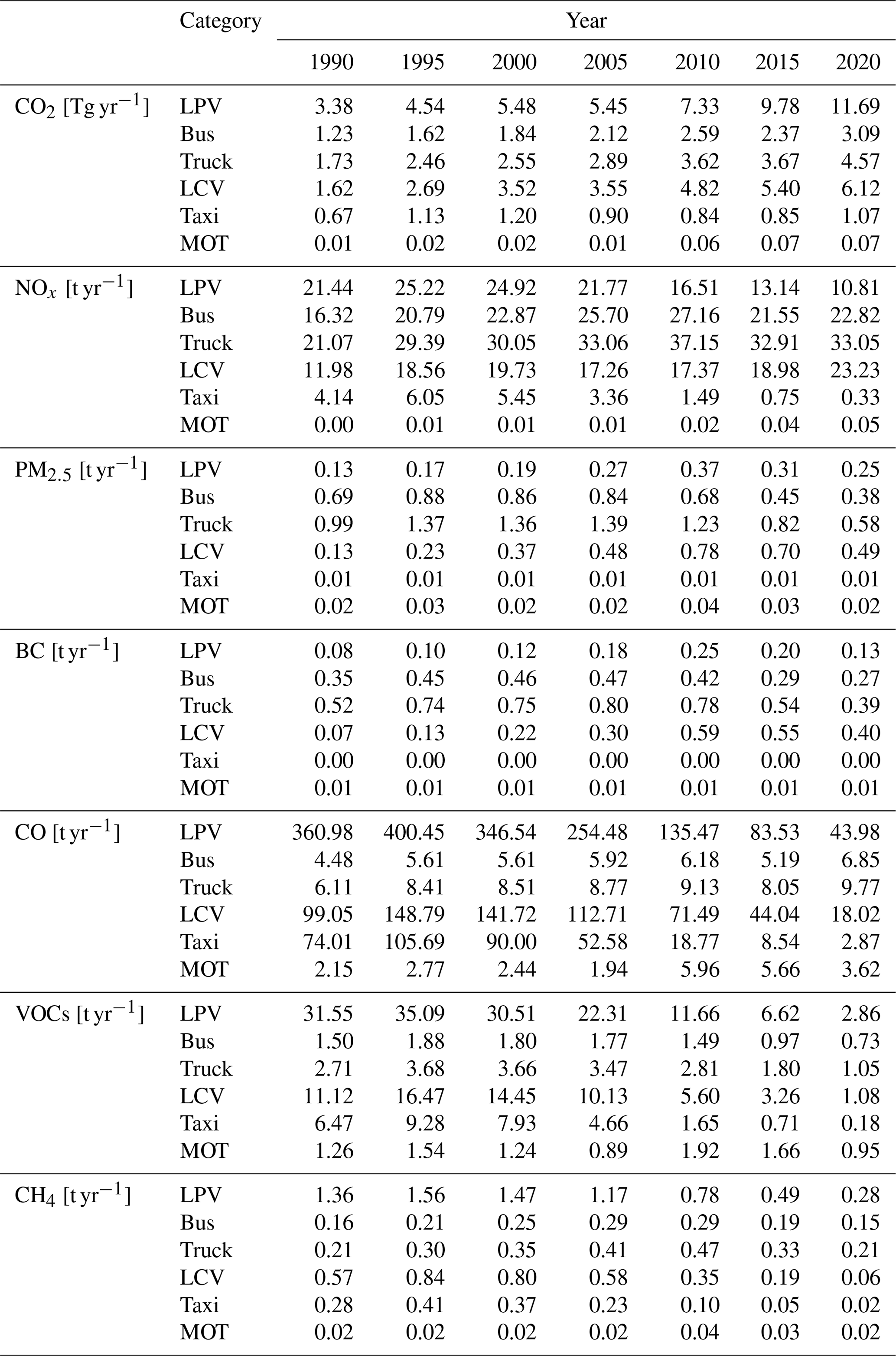
Table 7 and Fig. 5 show annual emission trends for six different compounds, divided by vehicle type. In the case of CO2 and NOx, all types of vehicle have relevant contributions (Fig. 5a and b); diesel vehicles are responsible for the majority of PM2.5 and BC emissions (Fig. 5c and d), and gasoline cars dominate CO and VOC emissions (Fig. 5e and f).
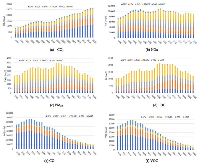
Except for CO and CO2, all annual emission curves show continuous growth from 1990 to 2006–2008. Thereafter, the general trend for local pollutants is to decrease. This turning point coincides with the change throughout the country in the requirement to go from Euro 1 to Euro 3 for light vehicles and from Euro II to Euro III for heavy-duty vehicles between 2005 and 2006 (Table 2). The limits for light gasoline vehicles for NOx, CO and VOCs between Euro 1 and Euro 3 are strict, which largely explains this change in trend. The change in PM2.5 in 2007 occurs immediately after the year 2006, when Euro III was imposed for buses in the most important regions of the country and Euro II was required for the first time from the rest of the public and private buses (previously many of them had no obligation to meet standards). Subsequently, during the years 2011–2014, Euro 4 and Euro 5 were required for light vehicles and Euro IV and Euro V for buses and trucks, which has allowed for continuing reducing emissions despite the growth in the vehicle fleet.
It is important to note that Chile has one of the most advanced state-owned vehicle homologation centres in Latin America (3CV Centro de Control y Certificación Vehícular, https://www.mtt.gob.cl/3cv.html, last access: 23 November 2021), which has controlled the entry of all new vehicles sold in the country since 1996. A 3CV emissions laboratory allows experimental verification of compliance with the regulations in force in Chile, according to European or United States procedures. Additionally, since 2007 the periodic technical inspection (PRT) procedure in Chile includes tests under load and simultaneously controls CO, HC and NOx for light vehicles and opacity for buses and trucks. The combination of both procedures, 3CV and PRT, are the main policy tools to enforce that the emissions of the vehicles that circulate in the country comply with the regulations in force at the time of their sale and during their lifespan.
From 2008 onwards, BC emissions have not been mitigated at the same rate as PM2.5, with the BC reduction being less effective, which can contribute to local health problems and negative effects on local climate change (Bond et al., 2013; WHO Regional Office for Europe, 2012). This can be explained given that the fraction for light vehicles decreases significantly when going from Euro 4 to Euro 5, but this is not the case for heavy vehicles, which have this significant decrease later, between Euro V and Euro VI (Table 4). Trucks and buses are the main contributors to the total emissions of BC, and these two categories are the latest to be required to comply with Euro VI. According to the information given in Table 4, the BC fraction in PM2.5 emissions for heavy-duty trucks is 75 % under Euro V, which is not a considerable reduction compared to other vehicle types.
Finally, all the emission curves show a drop in the 1999–2004 period, which is explained by the impact that the Asian financial crisis had on Chile, significantly affecting the sale of motor vehicles and their activity.
3.3 Spatial disaggregation
The complete database for the period 1990–2020 is available at the following DOI: https://doi.org/10.17632/z69m8xm843.2 (Osses et al., 2021). This inventory is part of the first gridded national inventory of anthropogenic emissions for Chile of criteria pollutants as well as of GHGs (hereafter INEMA from Spanish for Inventario Nacional de EMisiones Antropogénicas), presented by Álamos et al. (2022). INEMA comprises emissions for vehicular, industrial, energy, mining and residential sectors for the period 2015–2017 in Chile.
The spatial disaggregation of emissions at the national level shows the high concentration of emissions in urban areas and on main roads in the country. Figure 6 shows the fraction of PM2.5 emissions for the year 2020 over the cells of 0.01×0.01∘ of latitude and longitude, which is equivalent to approximately 1.11×1.11 km. It is difficult to clearly identify these emissions on the complete map of Chile due to its shape (Fig. 6a). However, when zooming in on each region, the populated areas with high emissions on the road network appear. Figure 6b shows the city of Antofagasta, which is approximately 22 km long and has a population of 388 thousand inhabitants, where most of the on-road vehicle activity is concentrated. Figure 6c corresponds to the metropolitan region with Santiago in the centre, where 7 million of the almost 19 million inhabitants of Chile live (INE, 2020). The same image shows the city of Valparaíso on the coast and Rancagua, south of Santiago. Finally, Fig. 6d shows the Biobío region, with the city of Concepción, which is home to 221 000 inhabitants.
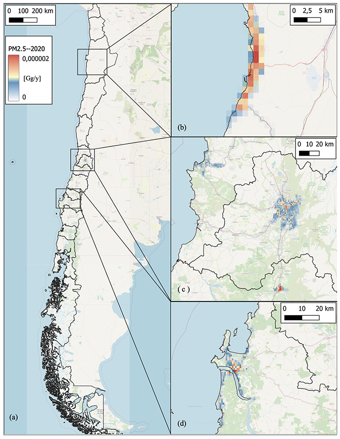
Figure 6Spatial disaggregation of PM2.5 exhaust emissions across the country (a), in Antofagasta (b), in the metropolitan region (c) and in Biobío–Concepción (d), 2020, as a fraction of Gg yr−1.
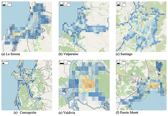
Figure 7Spatial disaggregation of NOx exhaust emissions for six cities in Chile, 2020, as a fraction of Gg yr−1. The colour legend is the same as in Fig. 6.
The images in Fig. 7 show the fraction of NOx emissions for the year 2020 in six major cities of Chile, from north to south. The emission grid is superimposed with the road network, green areas and uninhabited areas, obtaining a good match between them. In each city, the areas of greatest activity are coloured with warmer tones, indicating greater NOx emissions, decreasing towards colder tones for a lower fraction of these emissions.
3.3.1 Comparison with previous results
A direct comparison of emissions from this study with other emissions estimates was performed to reflect the differences in estimation approaches between local (bottom-up) and global (top-down) models, as well as the sensitivity to different assumptions in the estimates. Figures 8, 9 and 10 show the comparison among local estimates from this work – INEMA, the national emission inventory – INGEI (MMA, 2020) and an estimate using the LEAP model (Kuylenstierna et al., 2020) and global estimates by the EDGAR V5.0 global model (Janssens-Maenhout et al., 2017) – EDGAR, the CAMS-GLOB-ANT v4.2 dataset – CAMS (Granier et al., 2019), and the CEDS dataset – CEDS (McDuffie et al., 2020; Smith et al., 2015), for CO2, CH4, PM, BC, CO and NOx from 1990 to 2020 according to the pollutants available in each estimate. It is worth mentioning that EDGAR, CAMS and CEDS are not independent. For historic years CAMS is mostly based on EDGAR but extrapolated to more recent years using other information such as trends from CEDS.
CO2 and methane emissions are compared in Fig. 8. There is a good agreement in CO2 emissions and trends among most of the estimates for most of the period, which indicates that the activity level, i.e. fuel consumption, is consistent between top-down and bottom-up approaches. The largest difference is observed for the LEAP inventory from 2015, caused by a sudden reduction in 2015 and a slower increase between 2015 and 2020. Methane emissions show similar trends but different levels between this work (INEMA) and EDGAR from 1990 to 2004, global estimates being higher than the local estimate by 20 % to 43 %. The trends have become divergent since 2005, with decreasing emissions in the local estimate and increasing emissions in EDGAR, CAMS and CEDS. EDGAR and CAMS estimates were very similar between 2000 and 2011. Later, CAMS estimates increased linearly and more slowly than EDGAR emissions. On the other hand, EDGAR and CEDS estimates were the same between 2000 and 2014. Later, CEDS increased slightly more slowly than EDGAR. The decrease in the CEDS estimate between 2019 and 2020 is not reported in EDGAR.
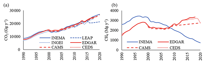
Figure 8Comparison between CO2 (a) and CH4 (b) between this work (INEMA) and other local and global emission inventories.
Figure 9 shows emissions estimates for PM and BC. With the exception of CEDS, there was a good agreement between local and global emission inventories between 1990 and 1998. However, EDGAR and CAMS show a sudden increase in 1999 that cannot be explained by a change in activity and is likely due to a change in the emission factors used in those inventories. Furthermore, after 1999, these global inventories show a consistent increasing trend. Such a trend was not followed by local estimates, which show a stabilization between 1997 and 2005 and a rather consistent decrease since 2007. As a result, EDGAR and CAMS PM (BC) emissions from 1999 to 2015 were between 85 % (87 %) and 315 % (208 %) higher than those from the local inventory. On the other hand, CEDS estimates for BC were even higher than EDGAR and CAMS estimates for the whole period, although they followed similar trends between 2000 and 2015. CEDS INEMA BC emission ratios range from 2.76 to 5.69, suggesting that BC emission factors in the CEDS dataset are significantly higher than those used in this work. Since this work's emission factors are based on the COPERT model and the actual vehicle technology distribution, higher PM and BC emission factors used in EDGAR and CEDS imply assumptions of an older fleet in global inventories. Standards for diesel vehicle emissions and sulfur fuel content have been greatly improved in Chile since 2000, so EDGAR, CAMS and CEDS emissions and increasing trends for PM and BC are likely overestimated.
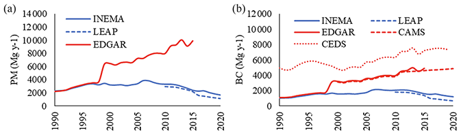
Figure 9Comparison of PM2.5 (a) and BC (b) emissions between this work (INEMA) and other local and global inventories.
CO and NOx emissions and trends are shown in Fig. 10. CO emissions were considerably higher in the global inventories (EDGAR, CAMS and CEDS) than in the local inventories (INEMA and LEAP), with a mean difference of 254 % (95 %–811 %), and the trends have been divergent since 2006, with increasing emissions in the global inventories and decreasing emissions in the local inventories. This is likely due to assumptions of an older fleet and, therefore, higher CO emission factors in the global inventories. A similar situation was observed for EDGAR and CEDS NOx emissions compared to local estimates, which showed rather similar levels between 1990 and 2005, with larger differences between 1993 and 1998, and diverged after 2005, with increasing emissions in the global inventories and decreasing emissions in the local inventories. Differences increased from 9 % in 2009 up to 70 % in 2015, with respect to local inventories. Once again, these differences suggest that global estimates did not reflect improvements in Chile's vehicle fleet after 2005.
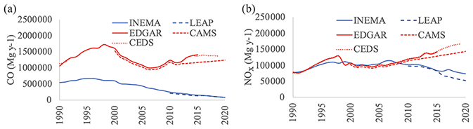
Figure 10Comparison between CO (a) and NOx (b) between this work (INEMA) and other local and global emission inventories.
Finally, the ratio and its trends are shown in Fig. 11, which includes not only Chile but also a comparison with European and two other countries in the Latin America and Caribbean (LAC) region between 1970 and 2020. The ratio was much higher in the global inventories than in the local inventories, with a mean difference of 209 % (90 %–457 %) between EDGAR and INEMA estimates for Chile and shows a decreasing trend in both, with more fluctuations in the global inventory. The differences in emissions and trends for CO and NOx suggest that global emission inventories use emission factors that correspond to technologies older than those that have been and are currently used in Chile. Considering the differences between EDGAR data and this study's results for Chile, trends in the ratio for other European and LAC countries from EDGAR were included. A big difference appears between these two groups of fleets, the ratio being much higher for selected LAC countries. In other words, according to EDGAR figures, LAC ratios reach European values 40 years later (1970 versus 2012), which seems inaccurate according to local estimates. Chile's ratios are in the same range as those found in European countries, which is supported by the fleet renewal shown in Figs. 3 and 4. Most of the Chilean fleet consists of Euro II/2 and Euro III/3 vehicles, which have much lower ratios than pre-Euro ones. Our analysis for Chile suggests that a careful analysis of national versus global estimates and/or emission factors for road transport emissions is needed for other LAC countries as well.
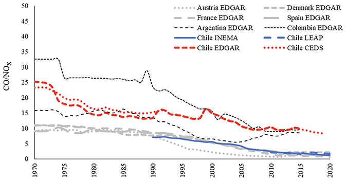
Figure 11 ratios for Chile and different countries from EDGAR and this work. External data obtained from the models EDGAR, CEDS and LEAP.
This dataset contains annual exhaust emission inventories of CO, VOCs, NOx, PM2.5, CO2, CH4 and BC from on-road transportation in Chile, for the period 1990–2020. The data are presented as netCDF4 files, in Gg yr−1 per cell for each species and year and gridded with a spatial resolution of 0.01∘ × 0.01∘ covering the domain 66–75∘ W and 17–56∘ S. It can be accessed through the open-access data repository https://doi.org/10.17632/z69m8xm843.2, under a CC BY 4.0 license (Osses et al., 2021).
This paper describes an original dataset for transport emission in Chile between 1990 and 2020, spatially distributed at 0.01∘ × 0.01∘. The dataset is based on annual reports from governmental agencies and estimates the evolution of air pollutants (CO, VOCs, NOx, PM2.5), greenhouse gases (CO2, CH4) and black carbon (BC). Results were contrasted with EDGAR, CAMS and CEDS datasets.
The analysis shows a significant growth in the vehicle fleet coupled with increasing CO2 emissions, which agrees with the national inventory of GHGs. Air pollutants show different patterns, with a general decreasing trend which coincides with pollution control measures. Data show a clear relationship between these emissions and the introduction of better fuel quality, due to a reduction in sulfur content and enforcement of technological improvements. These policy measures included regulation of emission standards for new vehicles into the fleet, mandatory periodic technical inspection for in-use vehicles and effective procedures for regulation enforcement.
The comparison with EDGAR, CAMS, CEDS and locally estimated datasets shows agreement in CO2 estimations and striking differences for local compounds, with global estimates consistently higher. This disagreement is likely due to differences in assumptions of vehicle technologies characterizing the fleet and quality of the fuel used. Trends between EDGAR and this transport dataset diverge in the case of PM and BC from 1998 and for CO, NOx and CH4 from 2006–2008. Results suggest that global emission inventories use emissions factors that do not coincide with the technologies of the vehicle fleet. EDGAR assumes a 40-year delay in technological updating for Latin American vehicle fleets compared to European ones, which is inaccurate for the case of Chile according to the dataset presented in this paper.
Every dataset has limitations, and this is not an exception; INEMA does not include cold-start emissions, and nor does it consider a calibration of fuel consumption according to vehicle age. The use of international emission factors is a second best compared to using locally measured emission factors, and COPERT does not cover ageing for all vehicle categories in the dataset. The impact of COVID-19 is not considered in 2020, but other studies have addressed its effects on urban emissions in Santiago (Toro et al., 2020). However, these limitations should not significantly change the results of the paper since the database provided is more accurate and extended than the existing ones, and the comparative analysis with external datasets shows differences that need attention.
This paper illustrates the potential of local datasets for policy ex post impact assessment. It also reinforces the value of available official raw data, produced with transparent methods and on a regular basis, as well as the production of national inventories. Further work could build on the dataset presented in this paper to produce projections and scenarios for future policymaking. Work should be carried out on the construction of local emission factors; this is the only information of the modelling that is not produced locally, and real emissions campaigns of a sample of the fleet could strengthen the results of this analysis.
NR contributed to the methodology, investigation, and writing – review and editing; CI contributed to the methodology, conceptualization, and writing – review and editing; VV contributed to the conceptualization and formal analysis; IL contributed to the methodology, formal analysis, data curation, and visualization; NP contributed to the data curation and visualization; DO contributed to the data curation and visualization; KB contributed to the methodology and review and editing; ST contributed to the methodology and review and editing; NH contributed to the review and editing; LG contributed to the review and editing; BG contributed to the methodology and data curation; MO contributed to the conceptualization, methodology, investigation, and writing – review and editing.
At least one of the (co-)authors is a guest member of the editorial board of Earth System Science Data. The peer-review process was guided by an independent editor, and the authors also have no other competing interests to declare.
Publisher's note: Copernicus Publications remains neutral with regard to jurisdictional claims in published maps and institutional affiliations.
This article is part of the special issue “Surface emissions for atmospheric chemistry and air quality modelling”. It is not associated with a conference.
The authors would like to acknowledge to the data providers of EDGAR V5.0 database, available at the EDGAR air pollutant website (https://edgar.jrc.ec.europa.eu/overview.php?v=_50_AP, last access: 23 November 2021). Also, we acknowledge developers of the CAMS dataset, described by Granier et al. (2019). Finally, data provided by the GEIA data portal ECCAD (https://eccad.aeris-data.fr/, last access: 23 November 2021) have been a great support for this study.
Institutional support and funding have been provided by the Center for Climate and Resilience Research (FONDAP no. 15110009), Technological Scientific Center of Valparaíso (ANID PIA/APOYO AFB180002), and the EU project Prediction of Air Pollution in Latin America and the Caribbean (PAPILA, ID 777544, H2020-EU.1.3.3.)
This paper was edited by Hugo Denier van der Gon and reviewed by two anonymous referees.
Álamos, N., Huneeus, N., Opazo, M., Osses, M., Puja, S., Pantoja, N., Denier van der Gon, H., Schueftan, A., Reyes, R., and Calvo, R.: High-resolution inventory of atmospheric emissions from transport, industrial, energy, mining and residential activities in Chile, Earth Syst. Sci. Data, 14, 361–379, https://doi.org/10.5194/essd-14-361-2022, 2022.
Barraza, F., Lambert, F., Jorquera, H., Villalobos, A. M., and Gallardo, L.: Temporal evolution of main ambient PM2.5 sources in Santiago, Chile, from 1998 to 2012, Atmos. Chem. Phys., 17, 10093–10107, https://doi.org/10.5194/acp-17-10093-2017, 2017.
BCN, Biblioteca del Congreso Nacional: Mapoteca, Mapas vectoriales webpage, https://www.bcn.cl/siit/mapas_vectoriales (last access: 23 November 2021), 2020.
Bond, T. C., Streets, D. G., Yarber, K. F., Nelson, S. M., Woo, J. H., and Klimont, Z.: A technology-based global inventory of black and organic carbon emissions from combustion, J. Geophys. Res.-Atmos., 109, 1–43, https://doi.org/10.1029/2003JD003697, 2004.
Bond, T. C., Doherty, S. J., Fahey, D. W., Forster, P. M., Berntsen, T., Deangelo, B. J., Flanner, M. G., Ghan, S., Kärcher, B., Koch, D., Kinne, S., Kondo, Y., Quinn, P. K., Sarofim, M. C., Schultz, M. G., Schulz, M., Venkataraman, C., Zhang, H., Zhang, S., Bellouin, N., Guttikunda, S. K., Hopke, P. K., Jacobson, M. Z., Kaiser, J. W., Klimont, Z., Lohmann, U., Schwarz, J. P., Shindell, D., Storelvmo, T., Warren, S. G., and Zender, C. S.: Bounding the role of black carbon in the climate system: A scientific assessment, J. Geophys. Res.-Atmos., 118, 5380–5552, https://doi.org/10.1002/jgrd.50171, 2013.
Burnett, R., Chen, H., Szyszkowicz, M., Fann, N., Hubbell, B., Pope, C. A., Apte, J. S., Brauer, M., Cohen, A., Weichenthal, S., Coggins, J., Di, Q., Brunekreef, B., Frostad, J., Lim, S. S., Kan, H., Walker, K. D., Thurston, G. D., Hayes, R. B., Lim, C. C., Turner, M. C., Jerrett, M., Krewski, D., Gapstur, S. M., Diver, W. R., Ostro, B., Goldberg, D., Crouse, D. L., Martin, R. V., Peters, P., Pinault, L., Tjepkema, M., van Donkelaar, A., Villeneuve, P. J., Miller, A. B., Yin, P., Zhou, M., Wang, L., Janssen, N. A. H., Marra, M., Atkinson, R. W., Tsang, H., Quoc Thach, T., Cannon, J. B., Allen, R. T., Hart, J. E., Laden, F., Cesaroni, G., Forastiere, F., Weinmayr, G., Jaensch, A., Nagel, G., Concin, H., and Spadaro, J. V.: Global estimates of mortality associated with long-term exposure to outdoor fine particulate matter, P. Natl. Acad. Sci. USA, 115, 9592–9597, https://doi.org/10.1073/pnas.1803222115, 2018.
Cai, H., Burnham, A., and Wang, M.: Updated emission factors of air pollutants from vehicle operations in GREETTM using MOVES, Syst. Assess. Sect. Energy Syst. Div. Argonne Natl. Lab., September, 2013.
Chow, J. C., Watson, J. G., Lowenthal, D. H., Chen, L. W. A., and Motallebi, N.: Black and organic carbon emission inventories: Review and application to California, J. Air Waste Manage., 60, 497–507, https://doi.org/10.3155/1047-3289.60.4.497, 2010.
Creutzig, F., Jochem, P., Edelenbosch, O. Y., Mattauch, L., van Vuuren, D. P., McCollum, D., and Minx, J.: Transport: A roadblock to climate change mitigation?, Science, 350, 911–912, https://doi.org/10.1126/science.aac8033, 2015.
Crippa, M., Oreggioni, G., Guizzardi, D., Muntean, M., Schaaf, E., Lo Vullo, E., Solazzo, E., Monforti-Ferrario, F., Olivier, J. G. J., and Vignati, E.: Fossil CO2 and GHG emissions of all world countries – 2019 Report, EUR 29849 EN, Publications Office of the European Union, Luxembourg, ISBN 978-92-76-11100-9, https://doi.org/10.2760/687800, JRC117610, 2019.
Crippa, M., Solazzo, E., Huang, G., Guizzardi, D., Koffi, E., Muntean, M., Schieberle, C., Friedrich, R., and Janssens-Maenhout, G.: High resolution temporal profiles in the Emissions Database for Global Atmospheric Research, Sci. Data., 7, 121, https://doi.org/10.1038/s41597-020-0462-2, 2020.
EEA, European Environmental Agency: Spreadsheet Appendix 4 to chapter '1.A.3.b.i-iv Road transport', EMEP/EEA air pollutant emission inventory guidebook 2019, Updated on 25 September 2020 and linked to COPERT v. 5.4, https://www.eea.europa.eu/publications/emep-eea-guidebook-2019/part-b-sectoral-guidance-chapters/1-energy/1-a-combustion/road-transport-appendix-4-emission/view (last access: 23 November 2021), 2020.
Gallardo, L., Barraza, F., Ceballos, A., Galleguillos, M., Huneeus, N., Lambert, F., Ibarra, C., Munizaga, M., O'Ryan, R., Osses, M., Tolvett, S., Urquiza, A., and Véliz, K. D.: Evolution of air quality in Santiago: The role of mobility and lessons from the science-policy interface, Elem. Sci. Anth., 6, 38, https://doi.org/10.1525/elementa.293, 2018.
Gallardo, L., Basoa, K., Tolvett, S., Osses, M., Huneeus, N., Bustos, S., Barraza, J., and Ogaz, G.: Mitigación de carbono negro en la actualización de la Contribución Nacionalmente Determinada de Chile: Resumen para tomadores de decisión, available at: https://www.cr2.cl/wp-content/uploads/2020/04/Mitigacion_carbono_negro_NDC_Chile2020.pdf (last access: 23 November 2021), Santiago de Chile, 2020.
Gobierno de Chile: Contribución determinada a nivel nacional (NDC) de Chile, Actualización 2020, https://www4.unfccc.int/sites/ndcstaging/PublishedDocuments/Chile irst/Chile's_NDC_2020_english.pdf (last access: 18 March 2022), 2020.
Gómez, B.: Modelación y proyección de emisiones contaminantes generadas por vehículos terrestres en el período 2020–2050 en Chile, Dissertation, Department of Mechanical Engineering, Universidad Tecnológica Federico Santa María, Chile, 2020.
Granier, C., Darras, S., van der Gon, H. D., Jana, D., Elguindi, N. The Copernicus Atmosphere Monitoring Service global and regional emissions (April 2019 version), Research Report, Copernicus Atmosphere Monitoring Service, https://doi.org/10.24380/d0bn-kx16, 2019.
Hadley, O. L. and Kirchstetter, T. W.: Black-carbon reduction of snow albedo, Nat. Clim. Change, 2, 437–440, https://doi.org/10.1038/nclimate1433, 2012.
Hardoy, J. and Romero Lankao, P.: Latin American cities and climate change: challenges and options to mitigation and adaptation responses, Curr. Opinion Environ. Sustain., 3, 158–163, https://doi.org/10.1016/j.cosust.2011.01.004, 2011.
Henríquez, C. and Romero, H.: Urban Climates in Latin America, Springer International Publishing, Cham, Switzerland, https://doi.org/10.1007/978-3-319-97013-4, 2019.
Huneeus, N., Denier van der Gon, H., Castesana, P., Menares, C., Granier, C., Granier, L., Alonso, M., de Fatima Andrade, M., Dawidowski, L., Gallardo, L., Gomez, D., Klimont, Z., Janssens-Maenhout, G., Osses, M., Puliafito, S. E., Rojas, N., Ccoyllo, O. S., Tolvett, S., and Ynoue, R. Y.: Evaluation of anthropogenic air pollutant emission inventories for South America at national and city scale, Atmos. Environ., 235, 117606, https://doi.org/10.1016/j.atmosenv.2020.117606, 2020a.
Huneeus, N., Urquiza A., Gayó, E., Osses, M., Arriagada, R., Vald s, M., Alamos, N., Amigo, C., Arrieta, D., Basoa, K., Billi, M., Blanco, G., Boisier, J.P., Calvo, R., Casielles, I., Castro, M., Chahu n, J., Christie, D., Cordero, L., Correa, V., Cort s, J., Fleming, Z., Gajardo, N., Gallardo, L., Gómez, L., Insunza, X., Iriarte, P., Labra a, J., Lambert, F., Muñoz, A., Opazo, M., O'Ryan, R., Osses, A., Plass, M., Rivas, M., Salinas, S., Santander, S., Seguel, R., Smith, P., Tolvett, S (2020). El aire que respiramos: pasado, presente y futuro – Contaminación atmosférica por MP2,5 en el centro y sur de Chile, Centro de Ciencia del Clima y la Resiliencia (CR)2, (ANID/FONDAP/15110009), 102 pp., 2020b.
INE, Instituto Nacional de Estadísticas: Official Statistics for population webpage, https://www.ine.cl/estadisticas/sociales/censos-de-poblacion-y-vivienda/poblacion-y-vivienda (last access: 23 November 2021), 2017.
Instituto Nacional de Estadísticas (INE): Censo 2017 de población y vivienda, bases de datos, https://www.ine.cl/estadisticas/sociales/censos-de-poblacion-y-vivienda/poblacion-y-vivienda, 2020.
Janssens-Maenhout, G., Crippa, M., Guizzardi, D., Muntean, M., Schaaf, E., Olivier, J. G., Peters, J. A. H. W., and Schure, K. M.: Fossil CO2 & GHG emissions of all world countries, Publications Office of the European Union, Luxembourg, https://publications.jrc.ec.europa.eu/repository/handle/JRC107877 (last access: 18 March 2022) 2017.
Jorquera, H., Cifuentes, L. A., Osses, M., Domínguez, M. P., Valdés, J. M., Cabrera, C., and Busch, P.: Apoyo a la iniciativa para el plan de mitigación de los contaminantes climáticos de vida corta en Chile, Ministerio de Medioambiente, Chile, https://www.greenlab.uc.cl/wp-content/uploads/2017/07/0-Resumen-Ejecutivo.pdf (last access: 18 March 2022), 2017.
Kirrane, E. F., Luben, T. J., Benson, A., Owens, E. O., Sacks, J. D., Dutton, S. J., Madden, M., and Nichols, J. L.: A systematic review of cardiovascular responses associated with ambient black carbon and fine particulate matter, Environ. Int., 127, 305–316, https://doi.org/10.1016/j.envint.2019.02.027, 2019.
Kuenen, J. J. P., Visschedijk, A. J. H., Jozwicka, M., and Denier van der Gon, H. A. C.: TNO-MACC_II emission inventory; a multi-year (2003–2009) consistent high-resolution European emission inventory for air quality modelling, Atmos. Chem. Phys., 14, 10963–10976, https://doi.org/10.5194/acp-14-10963-2014, 2014.
Kuylenstierna, J. C. I., Heaps, C. G., Ahmed, T., Vallack, H. W., Hicks, W. K., Ashmore, M. R., Malley, C. S., Wang, G., Lefèvre, E. N., Anenberg, S. C., Lacey, F., Shindell, D. T., Bhattacharjee, U., and Henze, D. K.: Development of the Low Emissions Analysis Platform – Integrated Benefits Calculator (LEAP-IBC) tool to assess air quality and climate co-benefits: Application for Bangladesh, Environ. Int., 145, 106155, https://doi.org/10.1016/j.envint.2020.106155, 2020.
MAPS Chile: Escenarios referenciales para la mitigación del cambio climático en Chile, Reporte Final Fase 1. Santiago de Chile: Ministerio del Medio Ambiente, https://mapschile.mma.gob.cl/lanzamiento-escenarios-referenciales-para-la-mitigacion-del-cambio-climatico-en-chile/ (last access: 23 November 2021), 2013.
Mazzeo, A., Huneeus, N., Ordoñez, C., Orfanoz-Cheuquelaf, A., Menut, L., Mailler, S., Valari, M., Denier van der Gon, H., Gallardo, L., Muñoz, R., Donoso, R., Galleguillos, M., Osses, M., and Tolvett, S.: Impact of residential combustion and transport emissions on air pollution in Santiago during winter, Atmos. Environ., 190, 195–208, https://doi.org/10.1016/j.atmosenv.2018.06.043, 2018.
McDuffie, E. E., Smith, S. J., O'Rourke, P., Tibrewal, K., Venkataraman, C., Marais, E. A., Zheng, B., Crippa, M., Brauer, M., and Martin, R. V.: A global anthropogenic emission inventory of atmospheric pollutants from sector- and fuel-specific sources (1970–2017): an application of the Community Emissions Data System (CEDS), Earth Syst. Sci. Data, 12, 3413–3442, https://doi.org/10.5194/essd-12-3413-2020, 2020.
Mena-Carrasco, M., Oliva, E., Saide, P., Spak, S. N., de la Maza, C., Osses, M., Tolvett, S., Campbell, J. E., Tsao, T. E. C. C., and Molina, L. T.: Estimating the health benefits from natural gas use in transport and heating in Santiago, Chile, Sci. Total Environ., 429, 257–265, https://doi.org/10.1016/j.scitotenv.2012.04.037, 2012.
Ministerio de Medio Ambiente (MMA): Cuarto Informe Bienal de Actualización de Chile sobre Cambio Climático, Ministerio del Medio Ambiente, Santiago, https://cambioclimatico.mma.gob.cl/wp-content/uploads/2021/01/Chile_4th_BUR_2020.pdf (last access: 23 November 2021), 2020.
Ministerio del Medio Ambiente (MMA): Informe del Inventario Nacional de Chile 2020: Inventario nacional de gases de efecto invernadero y otros contaminantes climáticos 1990–2018, Oficina de Cambio Climático. Santiago, Chile, 2021.
Ministerio de Obras Públicas (MOP): Peaje y pasadas vehiculares 2008–2020, Dirección de Vialidad, https://vialidad.mop.gob.cl/Paginas/PasadasVehiculares.aspx (last access: 23 November 2021), 2020.
Minjares, R., Wagner, D. V, Baral, A., Chambliss, S., Galarza, S., Posada, F., SHARPE, B., Wu, G., Blumberg, K., Kamakate, F., LLOYD, A., Kojima, M., HAMILTON, K., Johnson, T., Kopp, A., Hosier, R., and Akbar, S.: Reducing Black Carbon Emissions from Diesel Vehicles: Impacts, Control Strategies, and Cost-Benefit Analysis, Washington DC, https://www.ccacoalition.org/en/resources/reducing-black-carbon-emissions-diesel-vehicles-impacts-control-strategies-and-cost (last access: 23 November 2021), 2014.
Moreno, F., Gramsch, E., Oyola, P., and Rubio, M. A.: Modification in the Soil and Traffic-Related Sources of Particle Matter between 1998 and 2007 in Santiago de Chile, J. Air Waste Manage., 60, 1410–1421, https://doi.org/10.3155/1047-3289.60.12.1410, 2010.
Ntziachristos, L., Mellios, G., Fontaras, G., and Gkeivanidis, S.: Updates of the Guidebook Chapter on Road Transport, LAT Rep., 707, 65 pp., 2007.
Ntziachristos, L., Gkatzoflias, D., Kouridis, C., and Samaras, Z.: COPERT: A European Road Transport Emission Inventory Model, in: Information Technologies in Environmental Engineering, edited by: Athanasiadis, I. N., Rizzoli, A. E., Mitkas, P. A., and Gómez, J. M., Environmental Science and Engineering. Springer, Berlin, Heidelberg, 491–504, https://doi.org/10.1007/978-3-540-88351-7_37, 2009.
OSM, Open Street Maps: Webpage for Chile, https://wiki.openstreetmap.org/wiki/ES:Chile (last access: 23 November 2021), 2020.
Osses, M., Tolvett, S., and Henríquez, P.: Análisis y Desarrollo de una Metodología de Estimación de Consumos Energéticos y Emisiones para el Transporte. Report commissioned by Secretaria de Transporte, SECTRA, http://www.sectra.gob.cl/biblioteca/detalle1.asp?mfn=2800 (last access: 23 November 2021), 2010.
Osses, M., Tolvett, S., and Henríquez, P.: Actualización Metodológica del Modelo de Consumo Energético y Emisiones para el Sector Transporte (STEP), Informe comisionado por la Secretaria de Transporte, SECTRA, http://www.sectra.gob.cl/biblioteca/detalle1.asp?mfn=3236 (last access: 23 November 2021), 2014.
Osses, M., Rojas, N., Ibarra, C., Valdebenito, V., Laengle, I., Pantoja, N., Osses, D., Basoa, K., Tolvett, S., Huneeus, N., Gallardo, L., and Gómez, B.: High-definition spatial distribution maps of on-road transport exhaust emissions in Chile, 1990 – 2020, Mendeley Data V2 [data set], https://doi.org/10.17632/z69m8xm843.2, 2021.
Payri, F. and Desantes, J. M.: Motores de combustión interna alternativos, edited by: Payri, F. and Desantes, J. M., 1st Edn., Editorial Universitat Politècnica de València, Valencia, ISBN: 978-84-8363-705-0, 2011.
Ramanathan, V. and Carmichael, G.: Global and regional climate changes due to black carbon, Nat. Geosci., 1, 221–227, https://doi.org/10.1038/ngeo156, 2008.
Smith, J. S, Zhou, Y., Kyle, P., Wang, H., and Yu, H.: A Community Emissions Data System (CEDS): Emissions For CMIP6 and Beyond International Emission Inventory Conference, 101, 19395–19409, 2015.
Tolvett, S., Henríquez, P., and Osses, M.: Análisis de variables significativas para la generación de un inventario de emisiones de fuentes móviles y su proyección, Ingeniare, Rev. Chil. Ing., 24, 32–39, https://doi.org/10.4067/S0718-33052016000500005, 2016.
Toro, R., Catalán, F., Urdanivia, F. R., Rojas, J. P., Manzano, C. A., Seguel, R., Gallardo, L., Osses, M., Pantoja, N., and Leiva-Guzmán, M. A.: Air pollution and COVID-19 lockdown in a large South American city: Santiago Metropolitan Area, Chile, Urban Clim., 36, 100803, https://doi.org/10.1016/j.uclim.2021.100803, 2021.
USEPA: Emission Factor for Greenhouse Gas Inventories, U.S., https://www.epa.gov/sites/default/files/2018-03/documents/emission-factors_mar_2018_0.pdf (last access: 23 November 2021), 2018.
WHO Regional Office for Europe: Health effects of black carbon, Copenhagen, https://www.euro.who.int/en/health-topics/environment-and-health/air-quality/publications/2012/health-effects-of-black-carbon-2012 (last access: 23 November 2021), 2012.
Zheng, B., Huo, H., Zhang, Q., Yao, Z. L., Wang, X. T., Yang, X. F., Liu, H., and He, K. B.: High-resolution mapping of vehicle emissions in China in 2008, Atmos. Chem. Phys., 14, 9787–9805, https://doi.org/10.5194/acp-14-9787-2014, 2014.