the Creative Commons Attribution 4.0 License.
the Creative Commons Attribution 4.0 License.
 | 30 Nov 2021
INSTANCE – the Italian seismic dataset for machine learning
Alberto Michelini
Spina Cianetti
Sonja Gaviano
Carlo Giunchi
Dario Jozinović
Valentino Lauciani
The Italian earthquake waveform data are collected here in a dataset suited for machine learning analysis (ML) applications. The dataset consists of nearly 1.2 million three-component (3C) waveform traces from about 50 000 earthquakes and more than 130 000 noise 3C waveform traces, for a total of about 43 000 h of data and an average of 21 3C traces provided per event. The earthquake list is based on the Italian Seismic Bulletin (http://terremoti.ingv.it/bsi, last access: 15 February 2020) of the Istituto Nazionale di Geofisica e Vulcanologia between January 2005 and January 2020, and it includes events in the magnitude range between 0.0 and 6.5. The waveform data have been recorded primarily by the Italian National Seismic Network (network code IV) and include both weak- (HH, EH channels) and strong-motion (HN channels) recordings. All the waveform traces have a length of 120 s, are sampled at 100 Hz, and are provided both in counts and ground motion physical units after deconvolution of the instrument transfer functions. The waveform dataset is accompanied by metadata consisting of more than 100 parameters providing comprehensive information on the earthquake source, the recording stations, the trace features, and other derived quantities. This rich set of metadata allows the users to target the data selection for their own purposes. Much of these metadata can be used as labels in ML analysis or for other studies. The dataset, assembled in HDF5 format, is available at http://doi.org/10.13127/instance (Michelini et al., 2021).
- Article
(19373 KB) - Full-text XML
- BibTeX
- EndNote


Important breakthroughs in the understanding of earthquake phenomena can be achieved through the analysis of the very large number of continuous waveform recordings stored in the existing seismic archives. To this end, it can be important to make available well-organized representative subsets of the archives together with their associated metadata information.
The recent developments of machine learning (ML) software platforms like TensorFlow, PyTorch, Keras, Caffe (see Abadi et al., 2016; Paszke et al., 2019; Chollet and others, 2015; and Jia et al., 2014, respectively); the availability of high performance computing hardware (i.e., GPUs); and the access to thoroughly selected benchmark datasets (e.g., STEAD, https://github.com/smousavi05/STEAD, last access: 19 November 2021; and LEN-DB, https://doi.org/10.5281/zenodo.3648231) offer new opportunities to apply ML methodologies to seismological and earthquake engineering problems. In particular, the use of sophisticated and optimized ML algorithms for the analysis of large amounts of seismic data can lead to remarkable improvements for automated tasks like seismic waveform onset picking, ground motion prediction, and earthquake early warning; for the detection of hidden signals currently recognized as noise; or for novel modeling and inversion strategies (see Kong et al., 2018; Bergen et al., 2019; and Dramsch, 2020, for recent reviews). Specifically, the advent of ML in the field of seismology has highlighted the importance of reference datasets for benchmarking the developed methodologies, and it has fostered more thorough and statistically sound schemes for analyzing the data, like splitting all the available data into training, validation, and test sets. Moreover, the introduction of competitions like those for predicting laboratory earthquakes launched on the Kaggle platform (https://www.kaggle.com/c/LANL-Earthquake-Prediction/data, last access: 19 November 2021) or the SeismOlympics (Fang et al., 2017), which attracted several thousand teams, evidences even more the great potential of benchmark datasets (Johnson et al., 2021) and the general interest to tackle seismology problems with ML.
The application of ML techniques to seismological waveform data can be quite straightforward.
Indeed, large amounts of labeled data are already available thanks to the analyses carried out for many decades by expert analysts that have compiled and reviewed earthquake catalogs (which include phase onset readings, earthquake location, and size estimates)
or that have assembled ground motion parameters in special flat files and maps of strong ground motion among the most common tasks.
Their work provides effectively metadata that can be associated with the recorded waveforms and that can be used as labels when performing ML analysis.
A main bottleneck in wide-scale implementation of ML is, however, the fast access to the waveforms and to the associated metadata.
Open-access waveform archives available to the seismological community (e.g., EIDA, Strollo et al., 2021; or IRIS, Ingate, 2008)
were mainly designed for preserving the continuous data and making them available to the scientific community.
In practice, one of the main goals of seismological data centers has been the seamless acquisition of continuous data from the networks and the preservation, curation, and archiving of the entire record of continuous waveforms.
In this context, the users have complete flexibility in the selection of the data to download, but accessing large data volumes can be very time consuming.
Thus, despite the achievements attained in the last decades with the implementation of well-tested and efficient web services (e.g., FDSN dataselect), the accessibility of remote servers still remains cumbersome (Quinteros et al., 2021).
It follows that in order to attract a broader audience of users and developers there is a strong need to assemble and publish benchmark datasets that can be readily used with the existing software platforms (Mousavi et al., 2019).
In practical terms, the matter consists of assembling quality-checked data and metadata according to volume and formats ready to be used in ML applications.
Recently, effort has been made to assemble and make publicly available datasets consisting of waveforms and associated metadata. In detail, the dataset used in the works by Ross et al. (2018a), Ross et al. (2018b), and Meier et al. (2019) is downloadable from the Southern California Earthquake Data Center at the web portal https://scedc.caltech.edu/data/deeplearning.html (last access: 19 November 2021). This dataset includes 4.8 million time series recorded by nearly 700 receivers from more than 270 000 earthquakes in southern California. The STEAD dataset assembled by Mousavi et al. (2019) includes 1.2 million of 3C traces comprising 450 000 local earthquakes and 100 000 noise windows recorded by more than 2600 stations at the global scale. The LEN-DB dataset (Magrini et al., 2020) is also a global dataset of local earthquakes and includes 1.2 million 3C waveform traces, with half belonging to earthquakes and half to noise. The NEIC dataset (Yeck and Patton, 2020) includes global data and has been used by Yeck et al. (2020) to train the 1.3 million seismic-phase arrivals using three separate convolutional neural network models to predict arrival time onset, phase type, and distance.
Results attained by Ross et al. (2018b), L. Zhu et al. (2019), W. Zhu et al. (2019), Mousavi et al. (2020), and Mousavi and Beroza (2020) are excellent examples of successful applications of ML which can improve substantially the earthquake detection level with respect to most traditional methods, leading to the location of tiny and previously undetected earthquakes improving our knowledge on the heterogeneity of stress release on known and unknown faults. This enhanced information is crucial to make more thorough assessments of the ongoing seismotectonics and seismic hazard. The ML methods are likely to become an irreplaceable tool in seismology to extract as much information as possible from the large amount of data already stored in the archives. Among the indirect advantages, the enhanced detection can, to some extent, also govern network densification with sensible reductions in equipment investments and maintenance costs.
In general, the impressive performances of ML applications have been strongly related to the availability of large amounts of data with associated properly labeled metadata. Large amounts of data are critical to perform proper training and avoid data overfitting. However, the preparation of a ML dataset is also tedious and very time consuming. These are the main reasons that motivated the work presented in this article. Our goal is to provide an open-access dataset consisting of raw and instrument removed waveform data and associated metadata to study earthquake occurrence in Italy. The data collection, named INSTANCE, gathers seismic waveform data from weak- and strong-motion stations that have been extracted from the Italian EIDA node (Danecek et al., 2021; see Sect. 6 for a full list of the FDSN networks included in the dataset). The metadata associated with the waveforms are extracted from the INGV earthquake catalogue and from the waveform traces themselves. We expect this reference dataset to be used for several different purposes spanning from improvements of the existing configurations of seismic monitoring in Italy to the development and testing of new techniques for earthquake detection and ground motion estimation.
2.1 Data preparation
The data collection was assembled following the main stages listed below:
-
earthquake selection;
-
station selection;
-
waveform data selection and download;
-
cross-validation between phase-based station selection and downloaded waveform data;
-
processing of the data counts waveforms;
-
application of the instrument transfer function to the waveforms.
2.1.1 Earthquake selection
To compile the waveform dataset, we started from the Italian Seismic Bulletin (http://terremoti.ingv.it/en/bsi, last access: 15 February 2020, INGV bulletin hereinafter) and seismic stations archives (http://terremoti.ingv.it/iside, last access: 15 February 2020).
These data are public and can be queried using the fdsnws-event (https://www.fdsn.org/webservices/fdsnws-event-1.2.pdf, last access: 19 November 2021) and the fdsnws-station web services provided by INGV.
The event data belong to the INGV bulletin, which has been adopting the same velocity model and earthquake location software in the time period included in this study (see Appendix B for details).
The first step consisted of retrieving all the earthquakes with M≥0 from 1 January 2005 to 31 January 2020 in an enlarged area within the latitude and longitude corners (35.0, 5.0) and (49.0, 19.0). A total of 315 225 earthquakes were found. The beginning of the query corresponds approximately with the update, renovation, and increase in the number of stations of the national seismic network (Michelini et al., 2016; Danecek et al., 2021; Margheriti et al., 2021). Around 2005, the INGV network (FDSN code IV) underwent a major upgrade, with the existing, predominantly analog, instruments being replaced by high-quality digital seismic data loggers and new, mostly broadband (and some extended short period), three-component (3C) sensors. Selected stations were also complemented with additional 3C strong-motion sensors. The upgrade resulted in more than a 2-fold increase in the number of stations of IV network. In addition, since 2005, there have been many temporary deployments of seismic stations coinciding with earthquake sequences and specific experiments, the data of which are also available through the EIDA INGV node (Danecek et al., 2021). The total number of stations also increased thanks to the contribution of the networks belonging to other Italian institutions (e.g., the University of Genoa, the National Institute of Oceanography and Experimental Geophysics (OGS), and the University of Naples, among others). This increment resulted in a significant improvement of the detection of low-magnitude earthquakes. At the regional scale of Italy, the magnitude of completeness of the INGV bulletin is around ∼M 1.7–M 1.8, although significant differences occur depending on the area. In this regard, the preferred INGV catalogue magnitude is the local magnitude, Ml, (Richter, 1935) but sometimes also Mw and Md (see below for additional details).
A relevant aspect when compiling a large dataset to be used for ML purposes consists of gathering a balanced distribution of data. In seismology, when using earthquake magnitude for classification, balanced representation is impossible to achieve because small-size earthquakes, following the Gutenberg–Richter magnitude versus the number of earthquakes power law (Gutenberg and Richter, 1944), outnumber larger earthquakes. To address this issue (or at least to mitigate its influence), we choose to select in our target area
-
the great majority of the earthquakes with M≥4.0 – the earthquakes that have been discarded (30) all (except for 5) occurred outside the Italian country borders and mainly in the Balkan area (the earthquakes in Italy, all with M<5, will be included in a future update of the dataset);
-
earthquakes with origin times differing by more than 120 s in the range ; and
-
an additional 20 000 earthquakes, randomly selected, with origin times differing by more than 120 s for M<2.0.
The resulting distribution of the earthquakes according to their magnitude is detailed in Table 1, and they are mapped in Fig. 1a.
Table 1Final data selection. “All” indicates the total number of earthquakes in the INGV bulletin in the time period between 1 January 2005 and 31 January 2020, “Selected” and “Percent kept” refer to the earthquakes, and “Nb. 3C records” refers to the waveform traces included in the dataset.
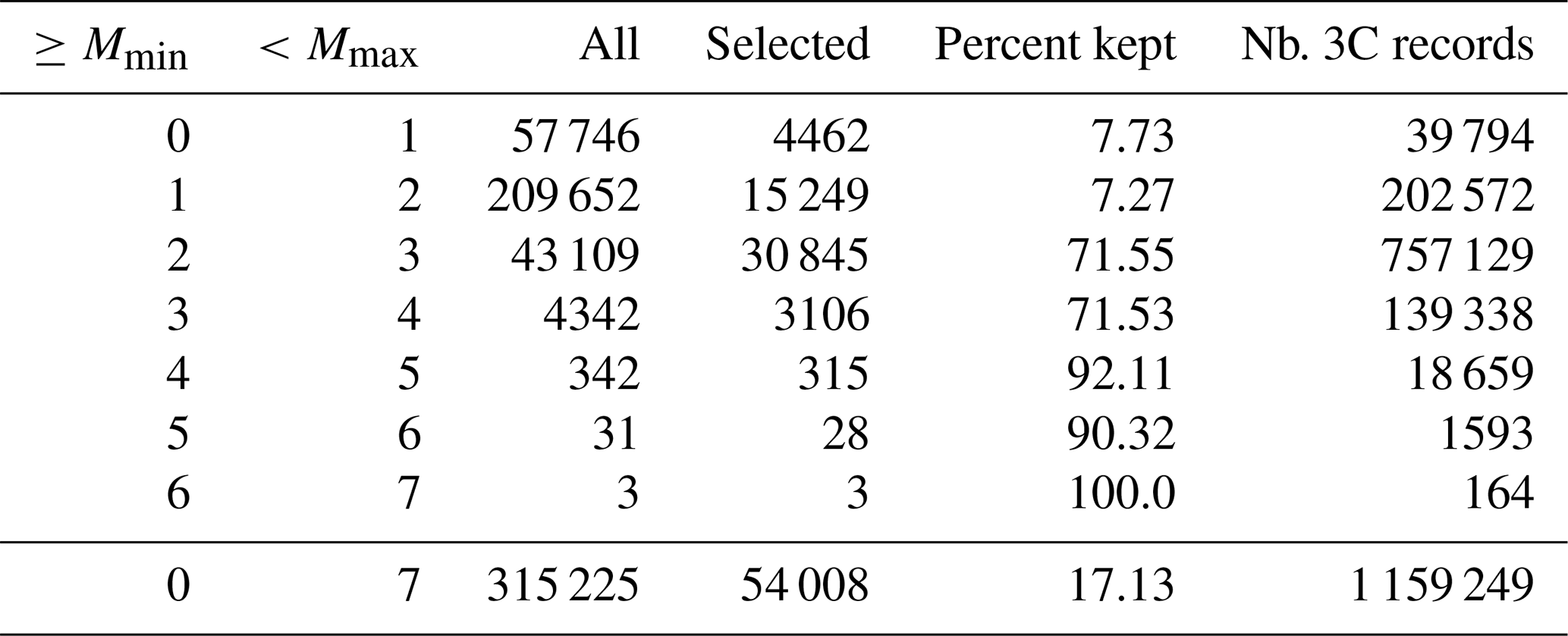
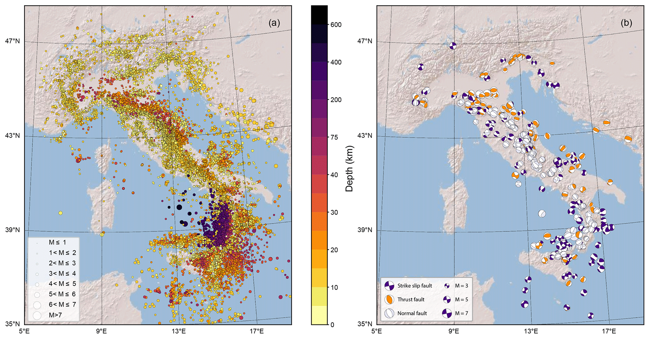
Figure 1Map of the earthquakes included in the dataset shown as solid circles with colors selected according to depth (a), and map of the available moment tensors with colors assigned depending on the focal mechanism (b). Symbol size, in both maps, is proportional to earthquake magnitude.
2.1.2 Station selection
In order to gather high-quality earthquake signals, we based our choice on the most accurately picked P- and S-wave onset phases published in the INGV bulletin. In this regard, the manual picking of the arrival phases is routinely performed by a group of about 20 INGV highly trained staff personnel who also review the hypocenter locations and magnitude determination before bulletin publication. These manually reviewed locations are indicated as preferred solutions in the INGV bulletin. In practice, we have selected only those stations that had P- and, if available, S-wave onset picks associated with the preferred location of the INGV bulletin. We note that the strong-motion data provided by the national strong-motion network (Rete Accelerometrica Nazionale) operated by the Italian Department of Civil Protection do not enter in the earthquake picking and location performed by the INGV staff, and the same data are not available through EIDA. They may be included, however, in future releases of the dataset.
In summary, we have adopted the following criteria to identify the waveform records to be included in the dataset after the earthquake selection above was applied:
-
all stations that feature P-wave onset phases (and S-wave onset phases when available) used for the preferred earthquake location (no distinction is made between Pg, and Pn and no secondary phases like PmP are picked);
-
all stations with waveform data available through the Italian EIDA node (see the dataset contributing networks in the pie diagram of Fig. 5b);
-
P- and S-wave location residual times less than 1.0 s;
-
P- and S-wave phases that contributed to the location with a weight larger than 10 %.
This selection procedure reduced the number of P- and S-wave phases from ∼1.9 to ∼1.2 and from ∼1.1 to ∼0.7 millions, respectively.
2.1.3 Waveform data selection and download
The selection procedure described in Sect. 2.1.2 resulted in the compilation of a list of waveform data time windows to be downloaded from the EIDA continuous waveform archive. We choose a time window of 120 s in order to include both P and S waves from stations whose distance is up to ∼600 km from the hypocenter. Indeed, in these cases, the S − P time differences are approximately 75–80 s. Adding about 20 s of the signal before the P-wave time and about 20 s after the S wave, we end up with a 120 s window choice providing the most significant earthquake signals for either the most distant stations, in the case of crustal depth earthquakes, or closer stations, in the case of deep earthquakes of the Calabrian Arc subduction.
More technically, the time windows set for data download were defined by inserting a randomly selected buffer time ranging between 15 and 20 s before the P-wave onset arrival phase and enlarging the time window to 125 s.
The adoption of 125 s long windows at the data download stage is arbitrary since after data processing the time windows have been all set to 120 s.
This criterion ensured that the great majority of the waveform traces downloaded featured a pre-P-wave onset buffer time between 15 and 20 s.
However, we found that, when dealing with such a large number of waveforms acquired by diversified instruments configured differently, some discrepancies may occur.
In practice, since the data
are archived in miniSEED compressed format that features different sizes of the logical records, and since the web service extracts the full logical record containing the predefined trace start time, the start time of the trace can be earlier than the predefined minimum time of 20 s (i.e., in this case, there is a longer time interval between the P-arrival and the actual trace start time).
In contrast, when data are missing before the P-wave onset time (i.e., in the 15–20 s pre-P-onset buffer time), start time of the extracted window can be delayed and a shorter time interval will separate the trace window start time from the P-wave arrival time (i.e., <15 s). See Fig. D1 in the Appendix for the distribution of the P- and S-wave phase arrival time samples.
The data (miniSEED format) were downloaded using the FDSN dataselect web services provided by INGV (http://terremoti.ingv.it/en/webservices_and_software, last access: 19 November 2021).
Using a set of 14 container-based querying procedures running in parallel, this stage required about 7 d to complete the download of the ∼4 million waveform traces (i.e., ∼1.3 million 3C traces), with a storage requirement of ∼80 GB (miniSEED STEIM1 compression).
2.1.4 Cross-validation between phases-based metadata and downloaded waveform data
After the massive data download was concluded, a list of all the downloaded files was generated. This list was intersected with the originally selected metadata (Sect. 2.1.2) to have a one-to-one correspondence between the miniSEED data and the metadata (i.e., each 3C waveform record – three miniSEED files – must correspond to a row of the metadata file).
2.1.5 Preparation of processed waveforms in digital units
This part of our data assembling procedure targets the preparation of the digital counts waveform traces. It includes the following steps:
-
removal of traces containing data gaps (i.e., missing data);
-
trimming the waveform trace to the nearest sample to the start time;
-
120 s trace windowing;
-
removal of mean and linear trends from the data;
-
resampling at 100 Hz;
-
calculation of the signal-to-noise ratio;
-
extraction of the data quality metrics.
No rotation of the horizontal component along the N–S and E–W directions was required since all sensors used are oriented accordingly. For each waveform trace (i.e., each component), the maximum value of signal-to-noise ratio (SNR) was extracted and kept as metadata. The SNR was calculated as
where and are the 95th percentile of the data absolute values in a 5 s window immediately after the S-wave onset and right before the P-wave arrival time. If the S-wave onset were not available, the S-wave window was determined after calculation of the predicted S-wave arrival using an average velocity of 3.0 km s−1 and the hypocentral distance.
During this stage of the data preparation, we have also calculated some quality parameters extracted from the waveform traces for the purpose of a later inclusion in the metadata information.
These additional parameters, providing the distribution of the trace values, have been computed using the MSEEDMetadata class of the ObsPy python software (Beyreuther et al., 2010; Megies et al., 2011; Krischer et al., 2015).
For the same purpose, we have determined the number of spikes using a Hampel filter on a 161-sample sliding window to find outliers in the traces.
The final dataset consists of a total of 1 159 249 3C waveform data records from 54 008 earthquakes in count units assembled within an HDF5 format file. Table 1 provides the number of traces within each magnitude interval of the final assembled dataset.
2.1.6 Application of the instrument transfer function to the waveforms
To make the dataset of more general use,
we have also generated a dataset in units of physical ground motion after deconvolving the instrument response.
To this end, we have downloaded the station response files for all the stations used and applied the transfer functions to
the individual traces with frequency filtering corners
0.01, 0.04, 25, and 40 Hz using a cosine flank frequency domain taper (see cosine_sac_taper in ObsPy) and applying a 5 % cosine tapering at both ends of the trace signal.
After removing the instrument response, we extracted the intensity measures (IMs, i.e., peak ground acceleration, PGA; peak ground velocity, PGV; and the spectral accelerations at a 0.3, 1.0, and 3.0 s period) on each component so that they could be included among the metadata parameters.
Peak ground displacements are not included since they are from single or double integration of velocity and acceleration records, respectively, and their determination can be inaccurate when performed automatically.
2.2 Metadata description
The 115 metadata associated with each 3C waveform trace of our collection are listed in Table 2. They provide different kind of information that can be subdivided into four main types – source, station, trace, and path metadata. The unit of each metadata is provided in its denomination.
The source metadata provide information on the earthquake with description of the source origin time; location; size; and, when available, the focal mechanism, the moment tensor, and the finite fault.
The station metadata provide information on the characteristics of the recording station, which include the station, channel, network, and location (SCNL) (cf. http://www.fdsn.org/seed_manual/SEEDManual_V2.4.pdf, last access: 19 November 2021); the geographical coordinates; and the average shear-wave velocity of the top 30 m of the Earth, VS,30, which is an important parameter for classifying sites in seismic engineering applications (e.g., Boore, 2004) and is extracted from the map used in the INGV implementation of the USGS ShakeMap software in Italy (Michelini et al., 2019).
The trace metadata consists of parameters that are extracted from the waveform traces like maximum and minimum amplitudes, root mean squared values of the traces, and, after application of the transfer function, intensity measures (IMs) of the ground motion. In this class of metadata, we include the P (and S wave) provided by the INGV bulletin and, in addition, the number of P and S picks obtained by processing the waveforms with two deep-learning, phase-picking and event-detection algorithms (GPD and EQTransformer; Ross et al., 2018a; Mousavi et al., 2020) to make the user aware that the waveform trace being used may include more than a single earthquake (see discussion further below).
The path metadata follow from the calculation of parameters that link the types of metadata above (e.g., traveltimes, hypocentral, and epicentral distances).
The rationale of our metadata selection reflects our intention of providing the users with comprehensive information about the data. This appears to be an important issue since the data, being recorded automatically, can suffer from many diverse problems deriving from malfunctioning of the data loggers and of the sensors or from poor data transmission. Since we seek to assemble a dataset that can be used also for analyzing real-time data streams using ML, we note that the automatic processing summarized above does not differ significantly from that routinely applied to the streamed data.
One alternative to our metadata comprehensive approach would have consisted of “cleaning” the dataset by removing the faulty traces from the dataset altogether. We do not think this approach is appropriate since in this case the dataset would not be representative of the “true” data that are collected in real time by the monitoring networks. Thus, the basic idea behind our criterion is that we would like to enable the users to make their own choices using opportune filters to exploit the data for their own purposes. For example, if a user looks for the cleanest data, this can be achieved by filtering the metadata accordingly (e.g., saturated velocimetric data acquired by broadband sensors equipped with 24 bit data loggers could be removed in a conservative fashion just by selecting only those traces with counts within ). In contrast, the user could also opt to leave the ML model to learn the data problems so that they can be detected when using real data. An approach of this kind has been used by Jozinović et al. (2020) for missing data. In Jozinović et al. (2020), the dataset used for ML consists of a fixed number of stations, and when data from one or more stations are missing (either the whole trace or parts of it), the signal trace is set to be an array of zeros. The ML model used there was found to detect and learn the problematic values, and compensate for them, having a similar prediction accuracy on those stations as the accuracy on the stations which had the input data available. In practice, the provision of a rich set of waveform descriptive metadata is important not only to make use of an enlarged suite of labels that can be used for diverse purposes but also to identify problems with the waveform data and include or filter them out.
Our metadata include P- and S-wave onsets manually picked by INGV analysts as provided in the INGV bulletin. Recall that the traces were selected to include just one P-wave arrival time and possibly one S-wave arrival time since we sought to assemble one earthquake per window trace. This criterion was chosen for the purpose of facilitating the training of ML models using traces containing just one earthquake (for phase picking, peak ground motions, etc.). However, even though we have made considerable efforts to isolate only one earthquake per time window, more than one can be present effectively within the same time window (e.g., the analyst did not see or just disregarded other events with smaller amplitudes). Because the presence of additional, unidentified earthquakes adds complexities to the ML training phase, we followed the same approach taken by Mousavi et al. (2019) to run automatic picking algorithms upon the waveform dataset and include as metadata also the number of P- and S-wave phases picked automatically by the generalized phase detection, GPD, technique proposed by Ross et al. (2018a) and the EQTransformer technique by Mousavi et al. (2020). In the analysis we have used as detection threshold 0.99 for P- and S-phase detection for GPD and 0.2, 0.1 and 0.1 for earthquakes, P-phase detection, and S-phase detection, respectively, for EQTransformer. Both GPD and EQTransformer have been run only on the high-gain channels (i.e., HH, EH).
As presented above, metadata are important constituents of data collections.
They can be used for identifying the data to be analyzed, and they can be used as labels in ML applications.
In addition to the fact that not all the metadata information in INSTANCE is always available (e.g., moment tensors are generally available only for events with magnitudes or the S-wave onset pick retrieved from the INGV bulletin may not be present), we have found that the automatically processed ground motion trace data may suffer from errors because the original traces contained already undetected malfunctioning problems (e.g., spikes, anomalous trends) which, after application of the instrument transfer function, are mapped into erroneous ground motion traces and IM values.
Similarly, it may have also occurred that in isolated cases the coefficients of the instrument transfer functions were incorrect, producing also in this case incorrect traces and IM values.
To address these problems, we have operated in two ways.
First, we have chosen to detect the traces' maximum and minimum values lying outside the acceptable physical range and to replace them with NumPy nan in the metadata file.
This acceptable range was based on the IMs reported in the “flat” file of the ESM DB (https://esm-db.eu/, last access: 19 November 2021, Lanzano et al., 2018), which includes all the IMs (obtained from analyst processing) of all the recordings available of earthquakes with M≥4.0 in Europe.
Secondly, we have verified our instrument transfer function processing procedure by cross-validating all our IM values with those reported in the ESM DB flat file.
In this regard, we found a very good correspondence between the IMs obtained using the two methodologies, giving us confidence in the quality of the applied data processing and of the IM metadata being provided.
Table 2List of the metadata for the events and noise waveform traces. The units are given in parenthesis in the “Description” column. Only a subset of metadata can be associated with the noise traces (star in the “Noise” column).

The horizontal line between “trace_EQT_number_detections” and “trace_[E,N,Z]_pga_cmps2” separates the additional metadata obtained after application of the instrument response transfer function.
2.3 Dataset description
Figure 1a shows the earthquakes included in the dataset. The symbol size is proportional to the earthquake magnitude. We observe that the 54 008 selected earthquakes composing the dataset can be considered a representative subset of the entire seismicity in Italy and, for the larger events, also for those earthquakes occurring in the near vicinity of the Italian national borders. During the time span of our data selection three important sequences occurred in Italy after the main shocks of the 2009 L'Aquila M 6.0 earthquake, the 2012 Emilia M 5.9 earthquake, and the 2016 central Italy extended sequence which featured three main earthquakes with magnitudes M 6.0, M 5.9, and M 6.5.
In Fig. 1b we plot the 527 moment tensors included in the metadata.
The size of the moment tensor symbol is proportional to source_magnitude, while the colors are defined according to the prevalent strain regime: indigo, lavender, and dark orange for strike slip, normal, and thrust faults, respectively. The prevalent strain regime is determined according to the fault's rake as derived from source_mechanisms_strike_dip_rake: strike slip for and , normal for , and thrust for .
In Fig. 2 we show the maps of the stations included in the events and noise datasets, respectively. The symbol size in panel a is proportional to the number of reported phase arrivals by each station, while in panel b it is proportional to the number of waveforms included in the dataset for each station. Figure 2a demonstrates that quite a different number of phases have been reported by the stations included in the event dataset. These differences depend on several factors like whether the stations are permanent or temporary, the time length of the acquisition, the noise level, and the level of seismicity of the area where the stations have been deployed. For example, it is evident that many stations in central Italy display many phases (and associated trace recordings) mainly because the area was struck by the 2009 and 2016 earthquake sequences. In contrast, stations that are located in the Po Plain generally feature a small number of phases mainly because the noise level is high, making the phase picking difficult. The same diversification in the number of available traces is not observable for the noise dataset shown in Fig. 2b. This occurs because it was an intentional choice to select a more or less even number of traces for all the station channels.
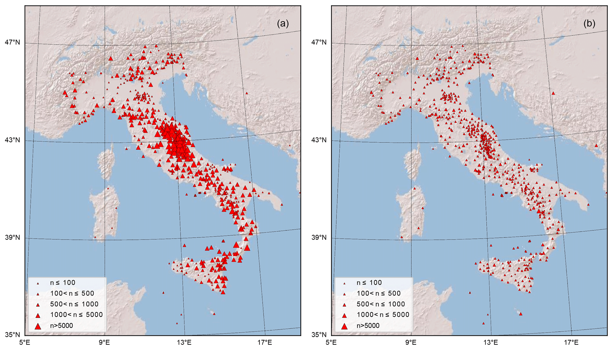
Figure 2Map of the stations used to assemble the events (a) and noise (b) datasets. The symbol size in panel (a) is proportional to the number of P phases and corresponding waveform traces available for each station. In panel (b) the symbol size is proportional to the number of traces. A total of 620 stations are included.
In Fig. 3, we show the distribution according to magnitude, earthquake to station epicentral distance, earthquake depth, and back azimuth of the 3C record traces composing the dataset. The panels show the histograms using the log 10 scale to provide a complete representation of the distribution of the dataset. We adopt the linear scale, however, to emphasize the distribution of the back azimuth in Fig. 3d. Despite the attempt to balance the distribution of earthquakes according to magnitude (Sect. 2.1.1), Fig. 3a shows that our selection still reflects (inevitably) the Gutenberg–Richter increase in the number of earthquakes at smaller magnitudes. The largest amount of trace records in the dataset belongs to earthquakes in the magnitude range . The significant decrease in the number of traces for M<2 follows from our choice to balance the dataset at small magnitudes by taking only about 7 % of the whole dataset. For what concerns the epicentral distances of the stations (Fig. 3b), the great majority of the traces have been recorded within 200 km. A better appreciation of the selected traces can be obtained from the observation of Fig. 4, where we show the magnitude versus hypocentral distance distribution of the dataset traces represented as density plots using hexagon binning (hexbin, Hunter, 2007). The earthquake depth distribution (Fig. 3c) shows that the great majority of the traces belong to shallow crustal earthquakes, although a few thousand occur in the depth range 100 to 300 km. At greater depths, the number of traces decreases sharply, and only a few hundred or fewer recordings are included in the depth range 400 to 550 km. Figure 3d shows that the great majority of the P- and S-wave onsets belong to paths more frequent along the NW–SE direction, in agreement with the geographical trend of the Apennines and of peninsular Italy overall.
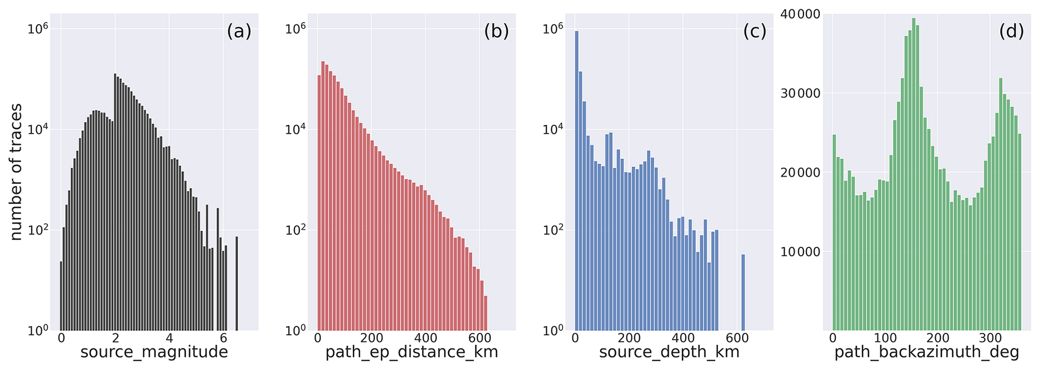
Figure 3Histograms of the distribution of the trace records composing the dataset according to magnitude (a), epicentral distances (b), earthquake depth (c), and back azimuth (d). The labels of the horizontal axis are assigned using the metadata names listed in Table 2.
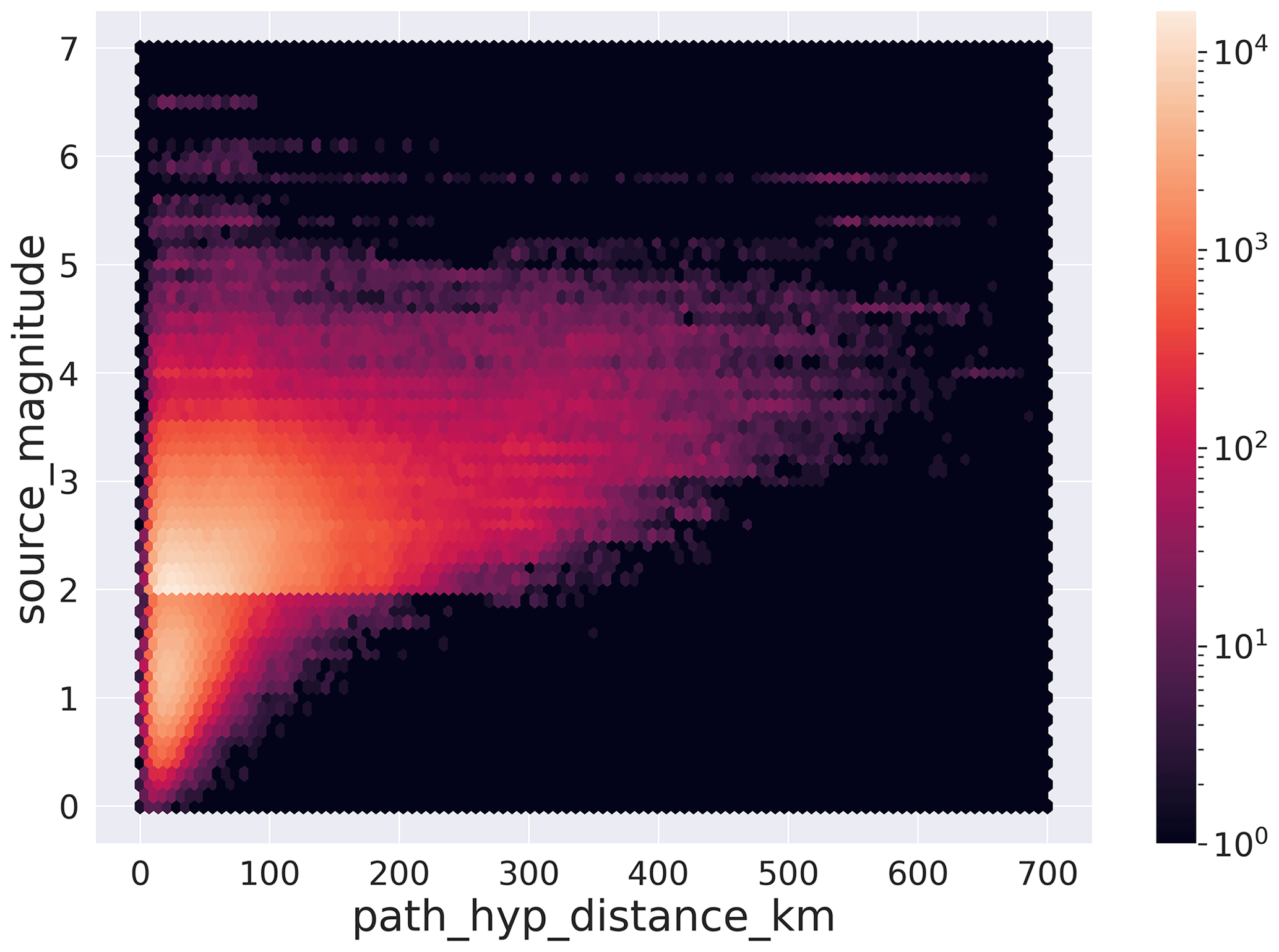
Figure 4Diagram of the earthquake magnitude distribution of the dataset versus receiver distance represented as a hexbin plot. The labels are assigned using the metadata names listed in Table 2.
Figure 5a shows the distribution of the trace channels of the dataset (station_channels).
The weak-motion, high-gain channels represent more than 70 % of the total number of traces.
These are subdivided into HH channels associated with the broadband high-gain velocimeters (51 %) of the total, whereas the extended-short-period channel (EH) traces account for 20 %.
The low-gain accelerometric channels form the remaining part of the dataset.
In Fig. 5b, we show the distribution of the records subdivided according to the different networks (station_network_code) operating in Italy and in neighboring countries that have been included in the dataset.
The dominant portion of the data (∼96 %) have been acquired by the Italian National Seismic Network (IV code) and by the MedNet (MN code), both operated by INGV (Michelini et al., 2016; Danecek et al., 2021).
The full list of the contributing networks is provided in the caption.
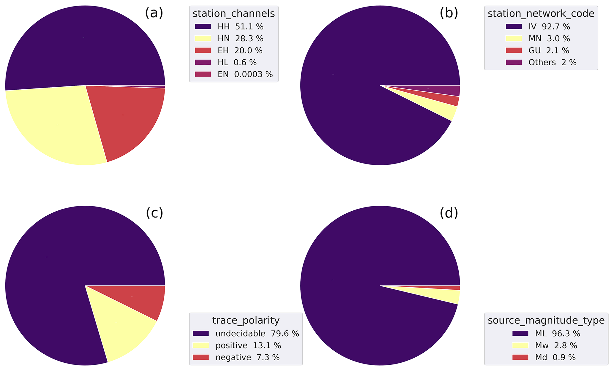
Figure 5Pie diagrams of the earthquake dataset summarizing the distribution of the channels (a), the data contributing networks (b), the P-wave polarities (c), and the magnitude types (d) of the dataset. The full list of station_network_code with %<1 collected in “Others” in decreasing order is OX, ST, SI, XO, NI, IX, OT, RF, YD, TV, B1, AC, HL, ZM, and 3A. See the metadata names listed in Table 2 for the specific metadata being represented.
The polarities associated with the P-wave onsets (trace_polarity) are shown in Fig. 5c and have been reported in only 20 % of the total number of traces.
Although this represents only a fraction of the dataset, we are confident that its number (∼235 000) is likely large enough to be used in a ML dedicated model (e.g., Ross et al., 2018b) for training and testing and then used to recover the polarities of the remaining batch.
In this regard, it is noteworthy to observe that the positive and negative polarities have a ratio of nearly 2:1. In Appendix C we have examined the possible origin for this asymmetry.
In addition, we would like to point out that, although the source_type is provided among the metadata, there are inherent difficulties to identify man-made sources by the staff analysts.
The magnitude type distribution (source_magnitude_type) is shown in Fig. 5d.
The Wood–Anderson local magnitude ML (Richter, 1935) is calculated predominantly (∼96 %).
The moment magnitude Mw is determined for earthquakes with and when enough good quality station data are available (Scognamiglio et al., 2009).
The Md magnitude is used only when it is impossible to determine the ML, and it is provided mainly in the first years of the dataset when the IV network still included a considerable number of analog stations.
In Fig. 6a and c we present the histograms of the P- and S-wave residual times included in the dataset. Figure 6b and d show the phase arrival weights resulting from the earthquake locations for P and S phases, respectively.
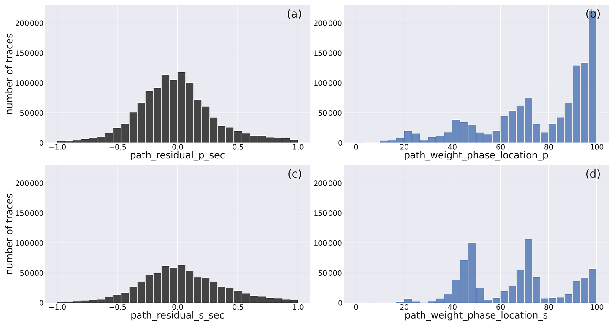
Figure 6Histogram of the P- and S-wave residuals (a, c) and of the preassigned phase arrival weights, expressed as percent, resulting from the location (b, d). The metadata names listed in Table 2 are used as labels for the specific metadata being represented.
To provide a broader perspective of the dataset and with the intent of showing the wide range of waveform paths that have been included, we present, in Fig. 7, the hexbin plots of the traveltime for both P- and S-wave arrival times used in the locations. These panels have been arranged using four different maximum distances and are useful for visualizing the dominant structure of the data selection given the large number of data.
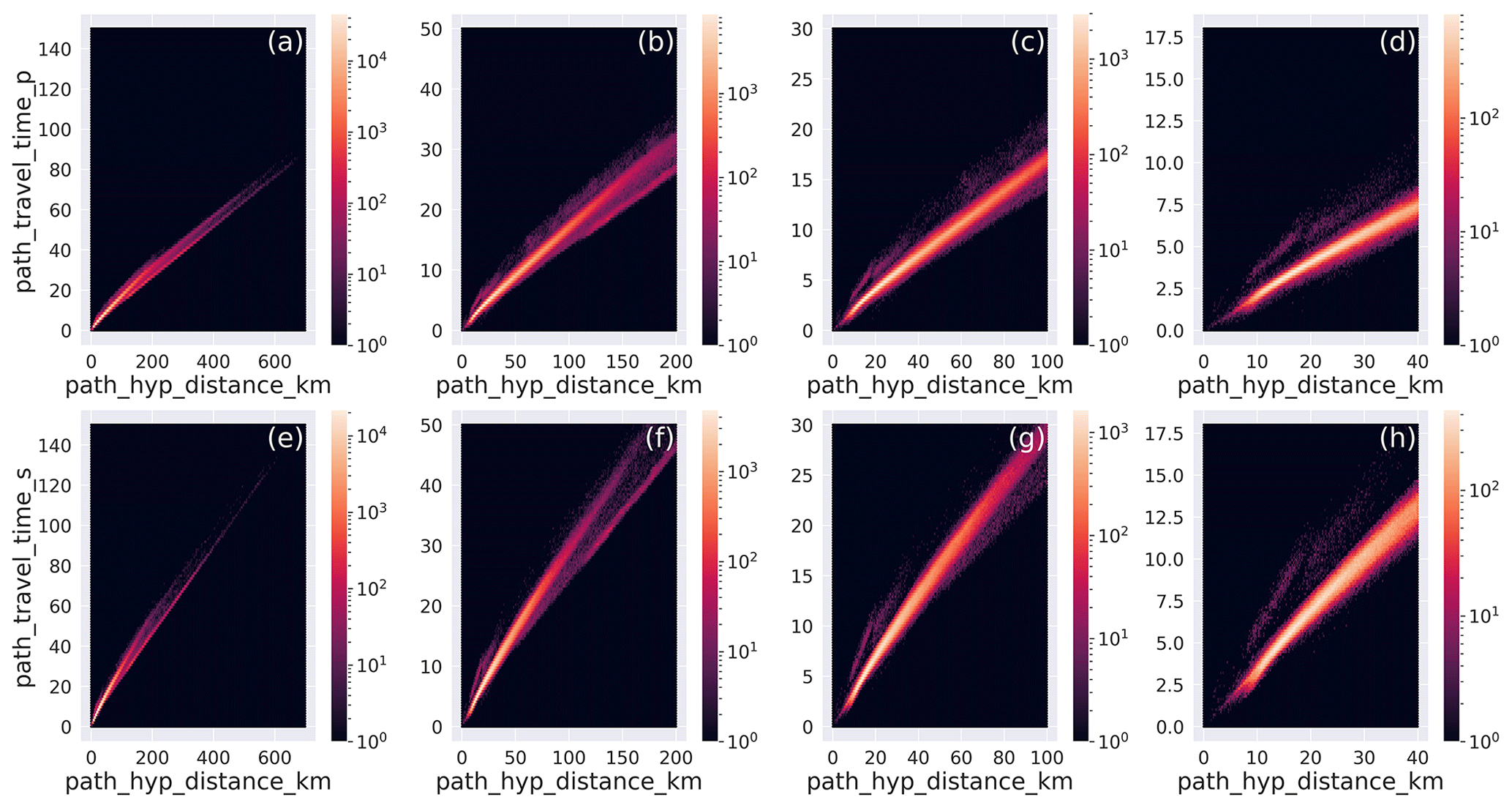
Figure 7Hexbin plot of the traveltimes for different hypocentral distance ranges for P (a–d) and S waves (e–h): (a, e) 0–700 km; (b, f) 0–200 km; (c, g) 0–100 km; (d, h) 0–40 km. The metadata names listed in Table 2 are used as labels.
More specifically, it can be observed that the hexagon binning panels for the larger distance ranges (700 and 200 km max distance) and for both P- and S-wave traveltimes (Fig. 7a, b, e, f) highlight well both the direct and the Moho refracted traveltimes. At smaller distance ranges (100 and 40 km, Fig. 7c, d, g, h), it is evident that our dataset includes waveforms that propagated across crustal structures with different velocities. This is very evident, for example, for both P and S waves in the hexbin plots, where at a small distance very low VP and VS velocities are observable.
In the following, we will focus on the trace amplitude metadata. These parameters are important for refined selection of the traces and are extracted from both the raw waveforms expressed in counts and from the traces in physical units after application of the instrument transfer function. Some of these parameters can be obtained without any knowledge on the earthquake source parameters, whereas others, like the SNR, require knowledge on the arrival times of P- and S-wave onset times.
The panels of Fig. 8 display the median (trace_[E,N,Z]_median_counts) and the mean values (trace_[E,N,Z]_mean_counts) of the dataset traces.
To evidence the whole range of values attained by these two metadata, we adopt the base-10 log scale.
The histograms show, for all the three components, remarkable differences of the distributions.
The mean values, which have been removed in the preprocessing preparation stage (cf. Sect. 2.1.5), are (obviously) centered about the zero value, whereas the median histograms, while being similarly centered about the zero value, do display a broader distribution of values around zero.
This last behavior occurs whenever the waveform trace values are unevenly distributed about the mean, and it derives from the preprocessing of faulty traces that, for example, result in defective removal of the linear trend.
The same figure for the full range of the parameters is available in Fig. D2.
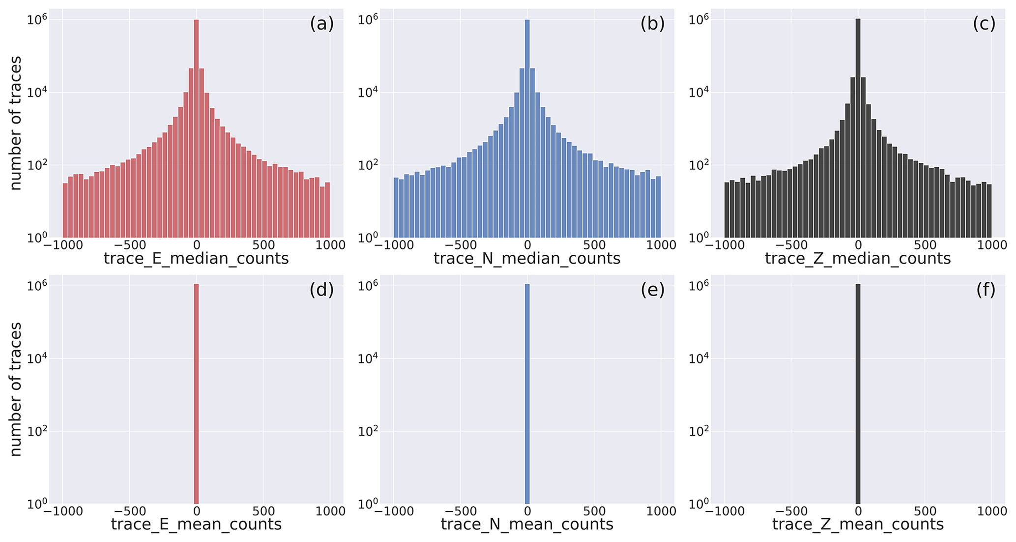
Figure 8Close view of the histogram of the distribution of the median and mean values of the E-, N-, and Z-component earthquake waveform traces. The full distribution is shown in Fig. D2. Note that the mean values (d–f) are shown to the sole scope of reference. The metadata names listed in Table 2 are used as labels for the specific metadata being represented.
In Fig. 9, we present the histograms of the distribution of the trace quality control parameters obtained from the application of the MSEEDMetadata module of the ObsPy seismological software suite.
The figure shows the distribution of the quality control parameters in a closer view (see the full range of values in Fig. D3).
The histograms show that the largest majority of the traces feature root mean square values less than 2.5×10⁴, with a minor contribution from traces featuring higher values.
The minimum and maximum values follow a similar trend for negative and positive values, respectively.
The lower- and upper-quartile values of the traces show that the peak of the distributions are at , respectively.
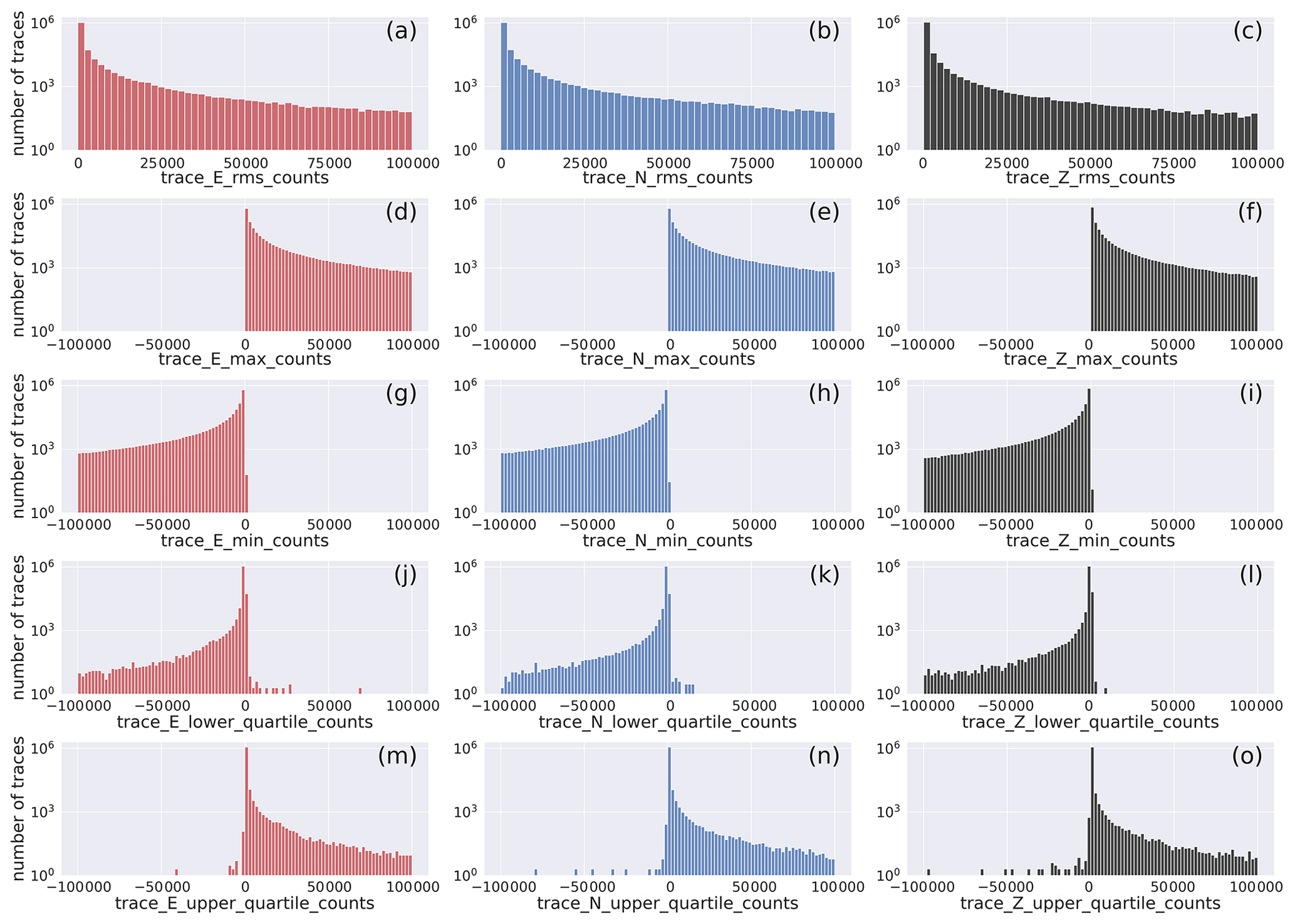
Figure 9Histogram of the distribution of quality control metadata of the earthquake E-, N-, and Z-component waveform traces: rms, min, max, and first and third quartile. The width of the bins is 2×10³. The full distribution of values is provided in Fig. D3. The horizontal axis labels correspond to the metadata being represented which are listed in Table 2.
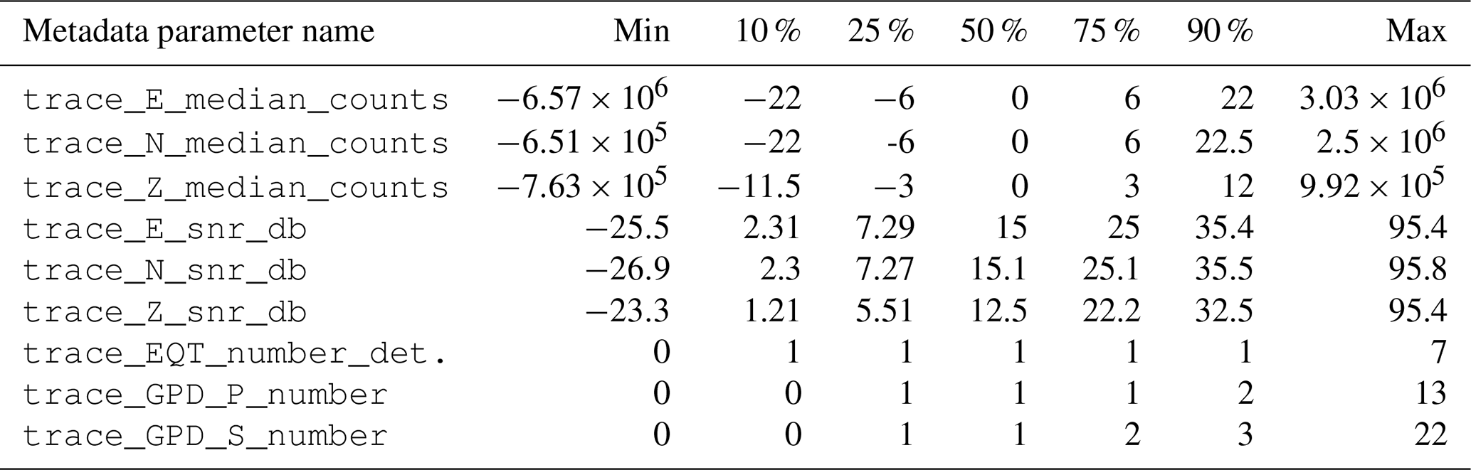
The SNR distributions are shown in Fig. 10 as histograms and versus distance and magnitude (M≥2) as hexbin plots in Fig. 11. The histograms show that the peak values for the whole dataset are at ∼10 db for the two horizontal components and slightly less for the vertical components (∼6 db). This is expected because the S-wave motion in the shallow, near-surface, low-velocity layers is polarized on a plane perpendicular to the nearly vertical propagation direction of the wavefront, implying that the ground motion occurs mainly along the horizontal components. In any event, the distribution of the SNR values of our dataset can be considered sensible given that values larger than 2 already provide distinct earthquake signals. In contrast and at the lower end of the SNR distribution, we find that 10 % (see Table 3) of the trace data of the HH channels have SNR values less than 2.3 (1.2 for the vertical component) that corresponds to roughly to 59 000 waveform traces out of the 592 000 traces of the HH channels included in the dataset. This number of low SNR traces could still be used, for example, to train ML models aimed at the detection of very small magnitude earthquakes slightly above the background noise level.
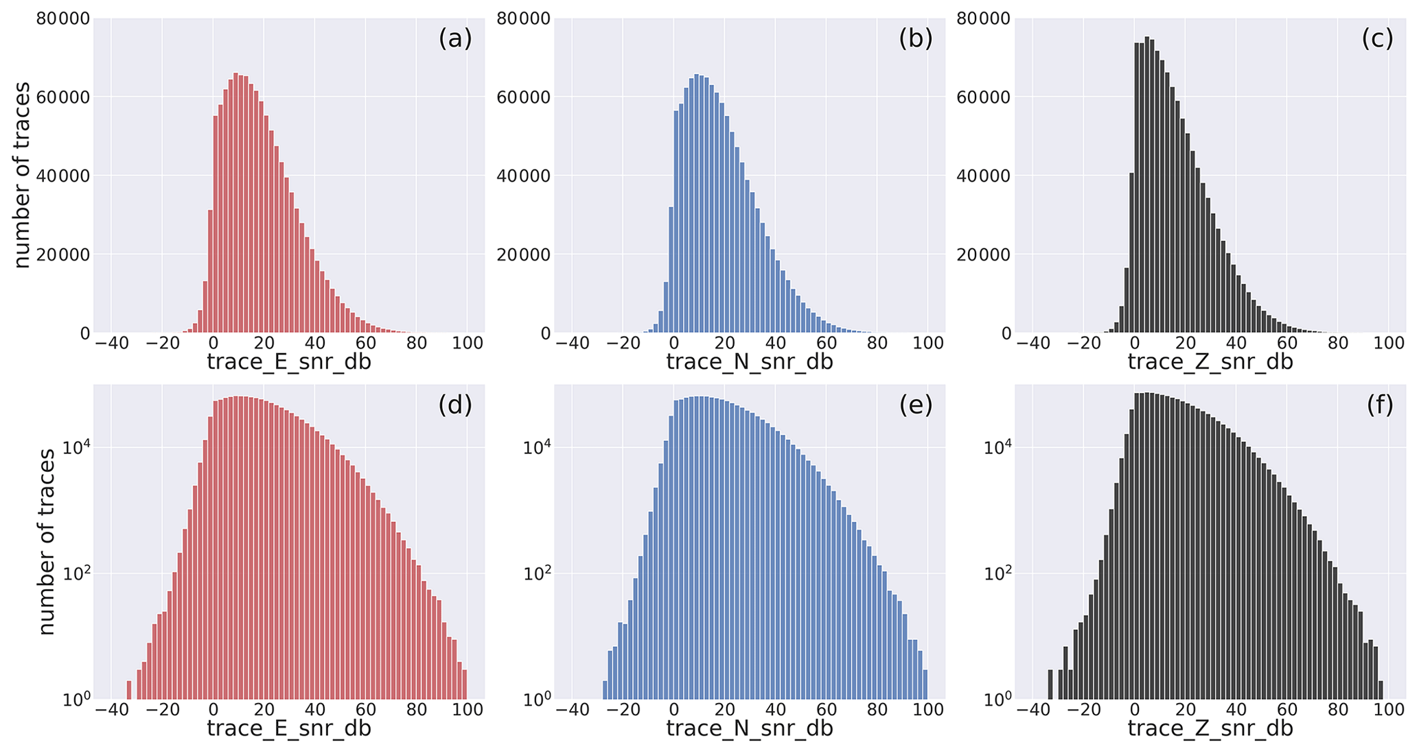
Figure 10Distribution of the signal-to-noise ratio of the earthquake E-, N-, and Z-component waveform traces. The panels (a)–(c) have linear y axes, whereas those on the bottom are in logarithmic scale. The horizontal axis labels correspond to the metadata being represented which are listed in Table 2.
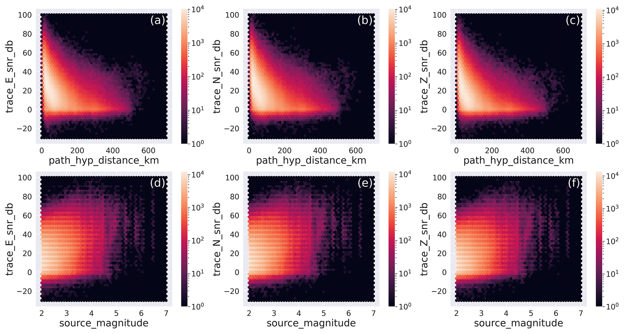
Figure 11Hexbin representation of the distribution of the signal-to-noise ratio for the E, N, and Z components of the earthquake dataset as function of hypocentral distance and magnitude. The metadata names listed in Table 2 are used as labels for the specific metadata being represented.
Table 3Distribution according to different quantiles of selected metadata (cf. Table 2) for the HH channels of the event dataset.
The hexbin plots of Fig. 11 provide a snapshot of the dominant levels of SNR with distance and magnitude. It is observed that higher values occur for nearby earthquakes and that the SNR progressively decreases at farther distances. Conversely and as expected, the SNR generally increases with larger-magnitude earthquakes.
The hexbin plots of the distribution of the IMs with distance for earthquakes with M≥2 are shown in Fig. 12, whereas their associated distributions are shown in Fig. D4. The panels evidence a broad concentration of ground motion values deriving from the inclusion of earthquake recordings from different distances and magnitudes. The panels also evidence some horizontal stripes at higher and lower values of ground motion resulting presumably from the acquisition and processing problems mentioned in Sect. 2.2.
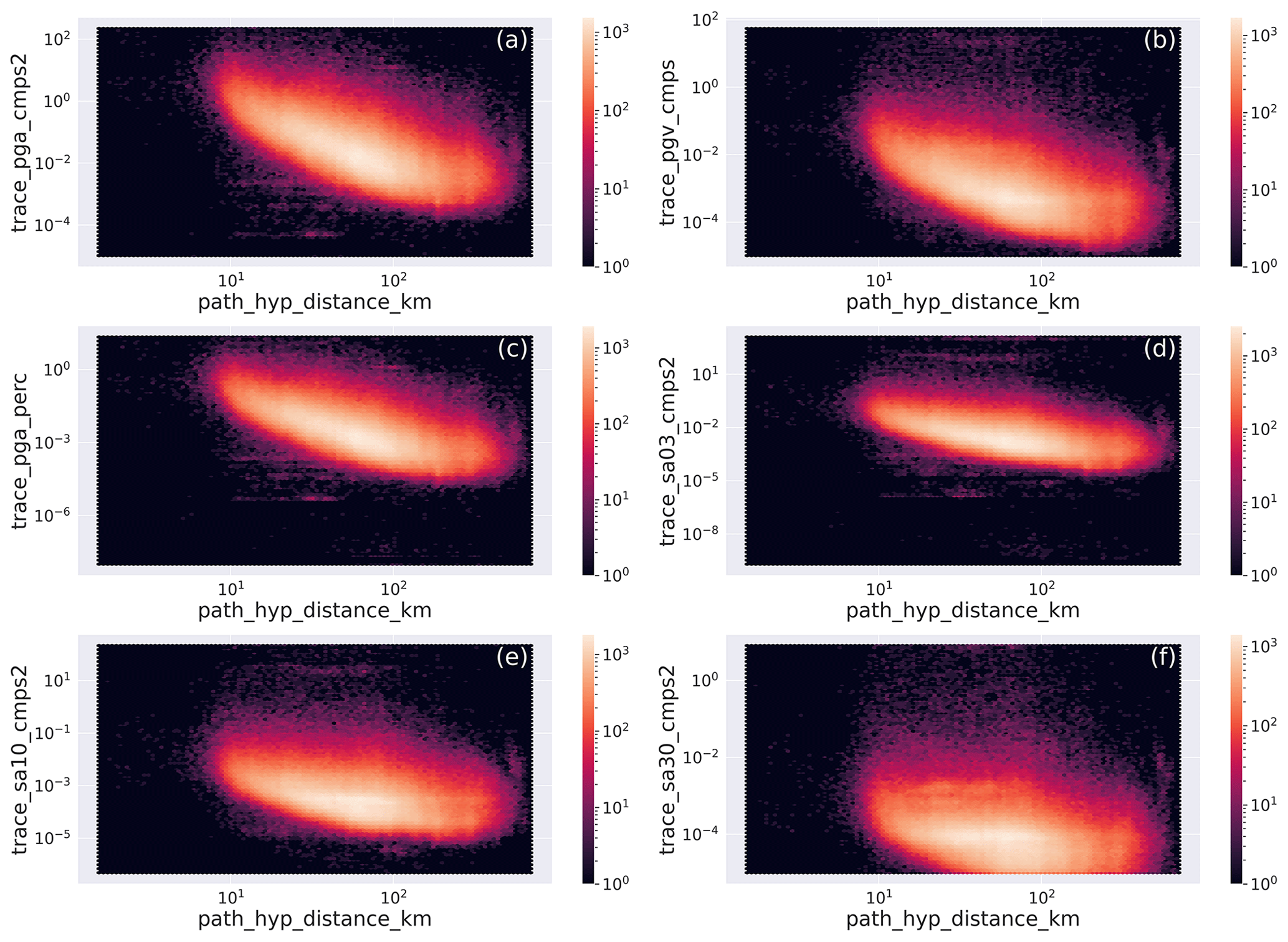
Figure 12Hexbin plot of the distribution of the intensity measures (IMs) with hypocentral distance of the earthquake dataset for the M≥2 earthquakes. The units are kilometers (km) along the horizontal axis in all panels, and along the vertical axis the units are centimeters per second squared (cm s−2) in panels (a) and (d)–(f), centimeters per second (cm s−1) in panel (b), and percent of the acceleration of gravity (% g) in panel (c). The metadata names listed in Table 2 are used as labels for the specific metadata being represented.
To show the distance dependence of the IMs for a given magnitude, in Fig. 13 we plot the values for M=3 earthquakes (i.e., IMs in the range ). The maximum concentration of IMs represent an average ground motion model for M=3 earthquakes in Italy.
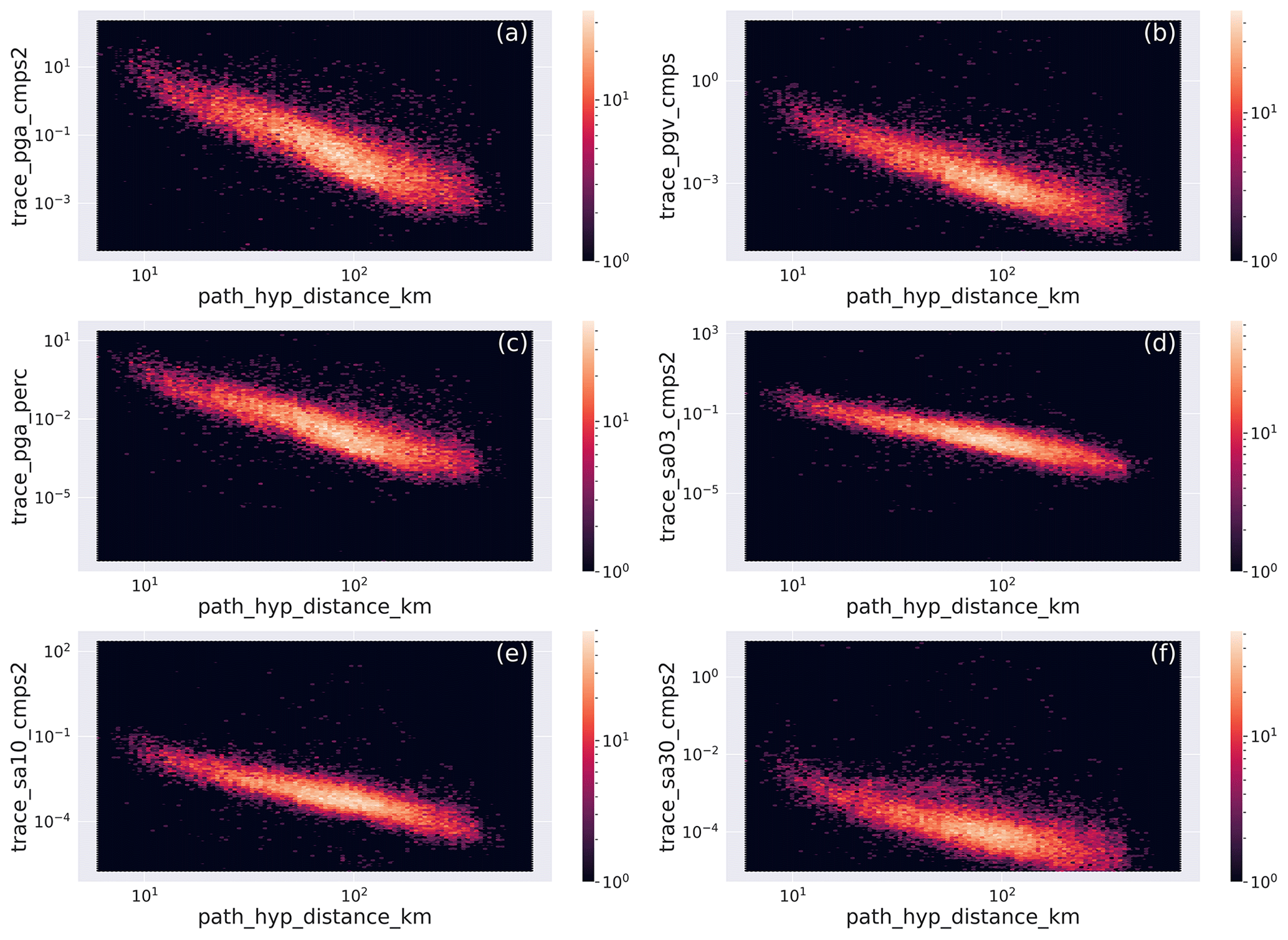
Figure 13Hexbin plot of the distribution of the intensity measures (IMs) with hypocentral distance for M=3 earthquakes. The units are kilometers (km) along the horizontal axis in all panels, and along the vertical axis the units are centimeters per second squared (cm s−2) in panels (a) and (d)–(f), centimeters per second (cm s−1) in panel (b), and percent of the acceleration of gravity (% g) in panel (c). The metadata names listed in Table 2 are used as labels for the specific metadata being represented.
2.4 Examples of event data traces
Some examples of the data traces are shown in Figs. 14, 15, and 16. The traces have been selected randomly according to certainly non-exhaustive criteria described in the figure caption using, as a guideline, the metadata distribution illustrated in Sect. 2.3.
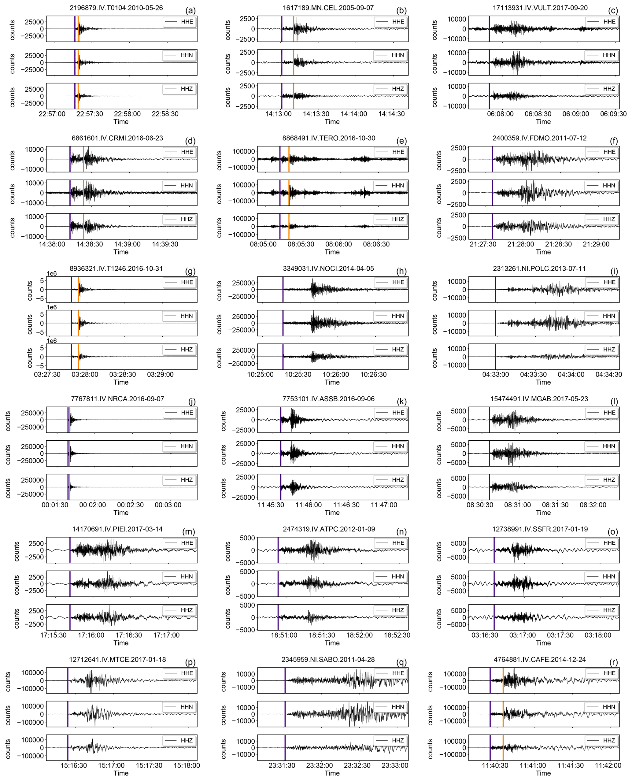
Figure 14Example of earthquake waveforms of the broadband HH channels contained in INSTANCE randomly drawn according to different criteria based on the metadata provided in Table 2.
Each row contains three, randomly selected, 3C traces based on the following criteria:
(a–c) earthquakes (66.8 % of the total of the HH channels);
(d–f) earthquakes (13.5 %);
(g–i) earthquakes M≥4 (2.0 %);
(j–l) earthquakes trace_E_snr_db ≥10 and path_ep_distance < 100 km (55.0 %);
(m–o) earthquakes trace_E_snr_db ≥10 and path_ep_distance ≥100 km (10.8 %);
(p–r) earthquakes M≥4 and trace_E_snr_db ≥10 (1.7 %).
The arrival times of P- and S-wave onsets (i.e., trace_[P,S]_arrival_time) are shown by indigo and dark orange vertical lines, respectively.
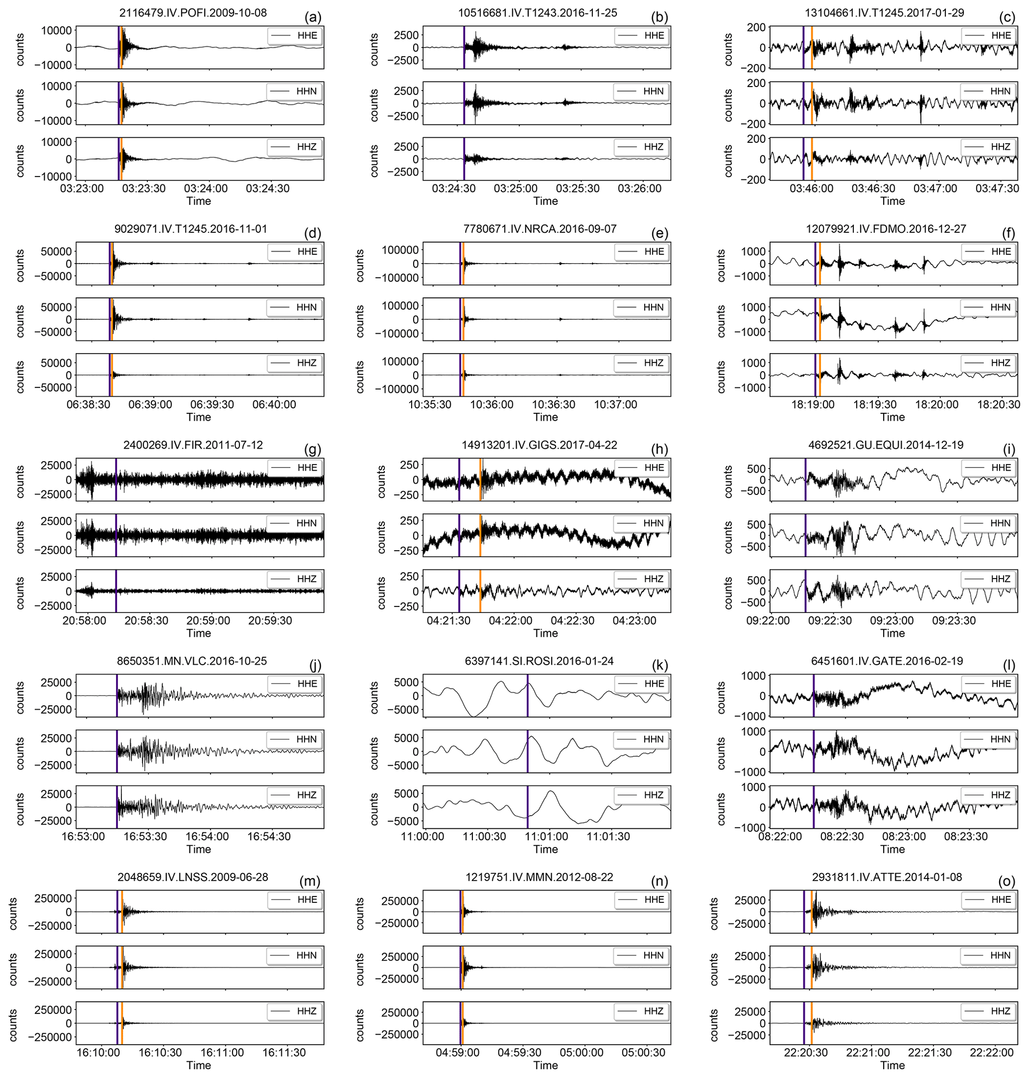
Figure 15Example of randomly selected “problematic” earthquake waveforms of the broadband HH channels. Each row contains three, randomly selected, 3C traces drawn according to the following criteria based on the metadata listed in Table 2:
(a–c) traces with trace_GPD_[P,S]_number >3 (7.96 % of the total of the HH channels);
(d–f) traces with trace_EQT_number_detections >3 (0.38 % of the total of the HH channels);
(g–i) traces trace_[ENZ]_snr_db with at least one component in the 10 % quantile (18.10 % of the total of the HH channels);
(j–l) traces with all trace_[ENZ]_median_counts either in the first 10 % or the last 10 % quantiles (5.90 % of the total of the HH channels);
(m–o) traces with trace_[ENZ]_median_counts either in the first 10 % or the last 10 % quantiles
and corresponding trace_[ENZ]_snr_db excluded from the first quartile (5.06 % HH dataset).
The arrival times of P- and S-wave onsets (i.e., trace_[P,S]_arrival_time ) are shown by indigo and dark orange vertical lines, respectively.
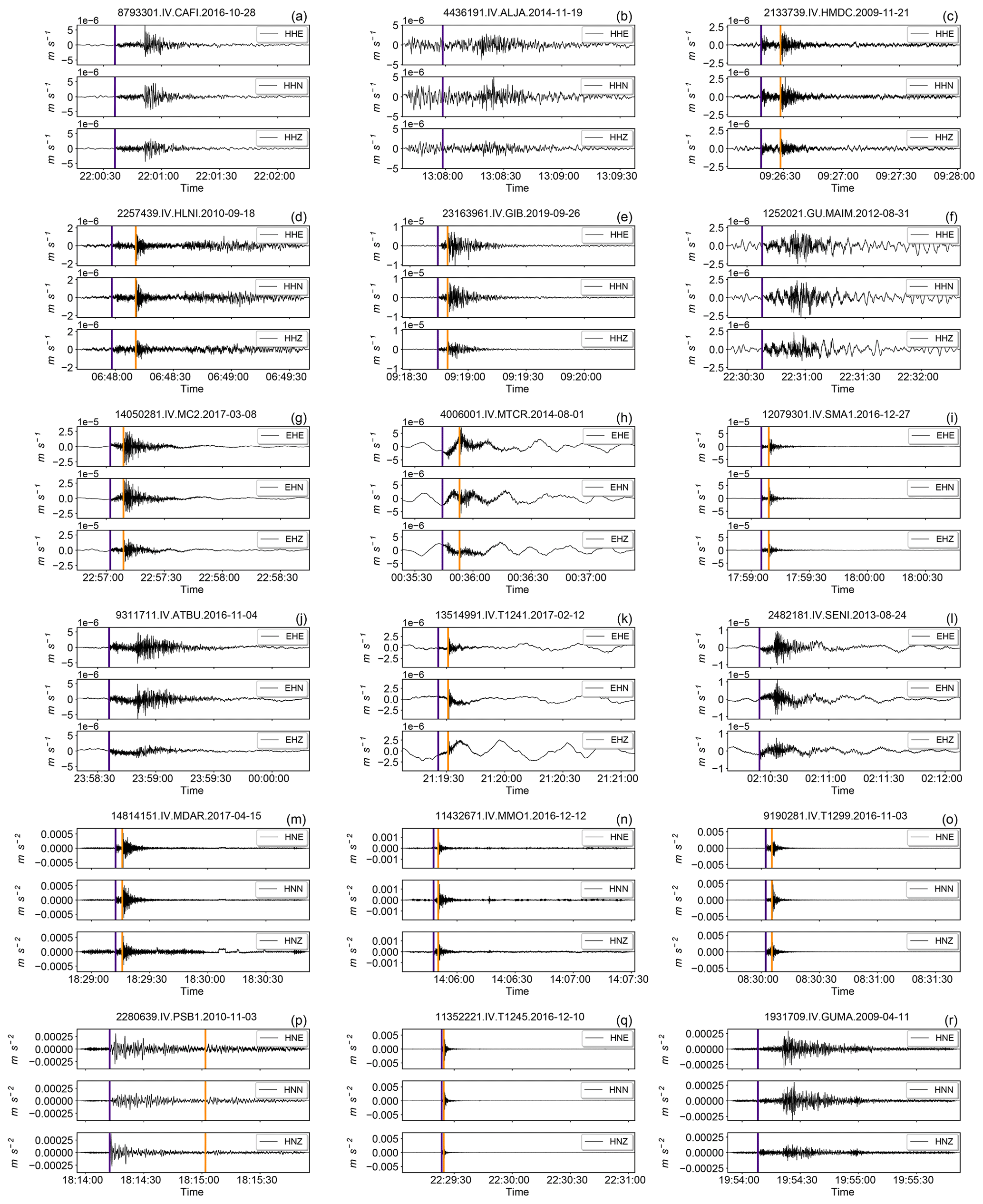
Figure 16Example of randomly selected event waveforms in ground motion physical units of the HH, EH, and HN channels in INSTANCE. The traces are representative of 75 % of the data and belong to the second, third, and fourth quartiles of each channel. Each row contains three, randomly selected, 3C traces drawn according to the following criteria based on the metadata listed in Table 2 and the quantile values provided in Table 4:
(a–f) HH traces with trace_pga_perc % g;
(g–l) EH traces with trace_pga_perc % g;
(m–r) HN traces with trace_pga_perc % g.
The arrival times of P- and S-wave onsets (i.e., trace_[P,S]_arrival_time) are shown by indigo and dark orange vertical lines, respectively.
In Fig. 14 we show the traces in counts of events recorded by the broadband instruments (HH channels). Specifically, the first three rows (Fig. 14a–i) show traces for different ranges of magnitude which, taken together, represent more than 80 % of the total HH traces. In the following two panel rows (Fig. 14j–o) we show examples of traces selected according to SNR and distance criteria that evidence that more than 65 % of the traces feature relatively high SNR (i.e., ≥10) within the whole distance range covered by our data collection. The seismograms shown in the last panel row (Fig. 14p–r) provide some samples of recordings of the largest events (M≥4) where we found that ∼87 % feature SNR ≥10.
To show how metadata can be used to isolate end-members of the dataset, we focus next on examples of problematic traces. Although different criteria could have been used given the comprehensive set of metadata available, here for simplicity we base our identification on (i) the number of picks and detections resulting from application of the GPD and EQTransformer algorithms to isolate those traces likely containing more than a single event, (ii) the value of the SNR to identify poor-quality noisy traces, (iii) the values of the trace median values which are expected to diverge from zero whenever the trace values are unevenly distributed about the mean value as result of acquisition or processing problems, and (iv) the values of peak acceleration and velocity ground motion parameters. The user, depending on desiderata, can customize the selection criteria. In Table 3, we provide a basic quantification of the distribution of the relevant metadata shown in Fig. 15, and, in Table 4, we present the distribution of the values of the maximum horizontal ground acceleration and velocity expressed as percent of the acceleration of gravity (% g) and centimeters per second (cm s−1), respectively. Some of the values reported in these two tables are used for our trace selections.
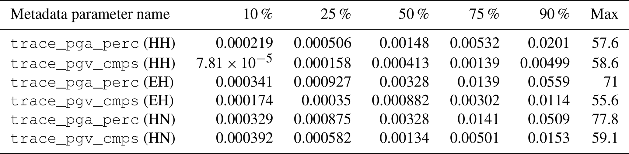
Table 4Distribution according to different quantiles of IM selected metadata for the HH, EH, and HN channels.
In Fig. 15a–c and d–f we show some traces that have been selected from the HH channels according to the number of P- and S-wave onset picks greater than three detected through the application of the GPD and EQTransformer techniques, respectively. Based on the values reported in Table 3, the presence of these multiple event traces in the dataset is less than the 10 %. In Fig. 15g–i, we focus attention on the traces that feature SNR values on at least one component within the lowest 10 % of the dataset. These traces are good examples of noisy traces and low-amplitude event signals. In Fig. 15j–l, we plot three traces for which the median values of all the three components fall within the two 10 % extremes. They represent about 6 % of the entire HH channels dataset. In the bottom row of Fig. 15m–o, we show that by excluding the very low 25 % of SNR values from the previous selection (Fig. 15j–l), it is possible to select traces that do not suffer of particular problems. In particular, we see that just by selecting a higher threshold of SNR values, about 85 % of the first and last 10 % of the distribution of median values, the traces appear acceptable.
In Fig. 16, we show the instrument-corrected traces randomly chosen in groups of six for each channel. The traces drawn from the entire dataset belong to the 75 % with the largest values of the maximum horizontal acceleration (i.e., second, third, and fourth quartile of the value distribution; see Table 4). The total of traces satisfying this criterion amounts to more than 860 000 3C traces. Application of the instrument transfer function appears to be generally successful without introduction of particular side effects with the exception of some amplification of the very low frequencies for some very low amplitude traces of the EH channels (e.g., panels h and k in Fig. 16). This effect results from our choice to bandpass filter all the traces channels in the same frequency range: this has the negative effect of boosting the low frequencies of the narrower-band EH channels, although it can be promptly removed by high-pass filtering. Overall, the quality of the ground motion unit dataset can be considered of satisfactory quality to perform analysis of ground motions.
Noise is generated by many different sources such as ocean waves, wind, traffic, instrumental noise, and electrical noise, and its suppression in earthquake recordings represents a long-standing objective (W. Zhu et al., 2019, and references therein). The inclusion of noise data in a dataset like INSTANCE is thus important because it provides information on the noise characteristics of the individual stations in the absence of earthquake-generated signal. ML models can reveal to be effective for noise removal or, in a classification analysis, for improving the detection of earthquakes. The noise data have been assembled starting from the stations gathered in the event selection stage described above.
3.1 Data preparation
Starting from the entire catalogue consisting of more than 300 000 events (Table 1), we first identified 600 s long time windows free of any earthquake. Secondly, we obtained the operational times of acquisition of each station. The third step consisted of identifying the 120 s time windows to be included in the dataset for each station and channel. This was achieved by intersecting the time window series obtained in the previous two stages (i.e., the event-free windows and the periods of station acquisition). It follows that the adopted procedure does not entail the selection of the same time window for multiple stations. For stations acquiring more than one channel type (e.g., HH and HN), noise windows for all the channels were identified and downloaded. The resulting total number of noise trace windows is 132 288, corresponding to about 10 % of the total number of traces of INSTANCE. We note also that this procedure does not preclude the presence of noise traces that include energy from regional and teleseismic events.
3.2 Metadata description
The 46 metadata elements (Table 2) used for the noise data selection include for each 3C waveform trace an identifier based on the start time, the station parameters, the trace quality control that includes the automatic picks, and event detection obtained using the GPD and EQTransformer procedures. These picks provide potential insights on whether any earthquake not catalogued in the INGV bulletin might be present in the selected time windows.
In Fig. 17 we show the channel subdivision of the downloaded noise together with the networks the stations belong to.
In Figs. 18 and 19, in analogy with what is presented for the event data, we present the trace characteristics of the metadata.
The trace_[E,N,Z]_mean_counts and trace_[E,N,Z]_median_count provide an outlook on the distribution of the mean and median values, and likewise the same parameters extracted from the event traces could be used to identify high-quality data.
The histograms of the trace_[E,N,Z]_rms_counts noise values fall mainly in the range of values from 0 to 2000 counts with similar peak values for either trace_[E,N,Z]_max_counts or trace_[E,N,Z]_min_counts.
This all would suggest that the gathered noise traces are of fairly good quality responding to the expectation of traces characterized by amplitudes with small number of counts.
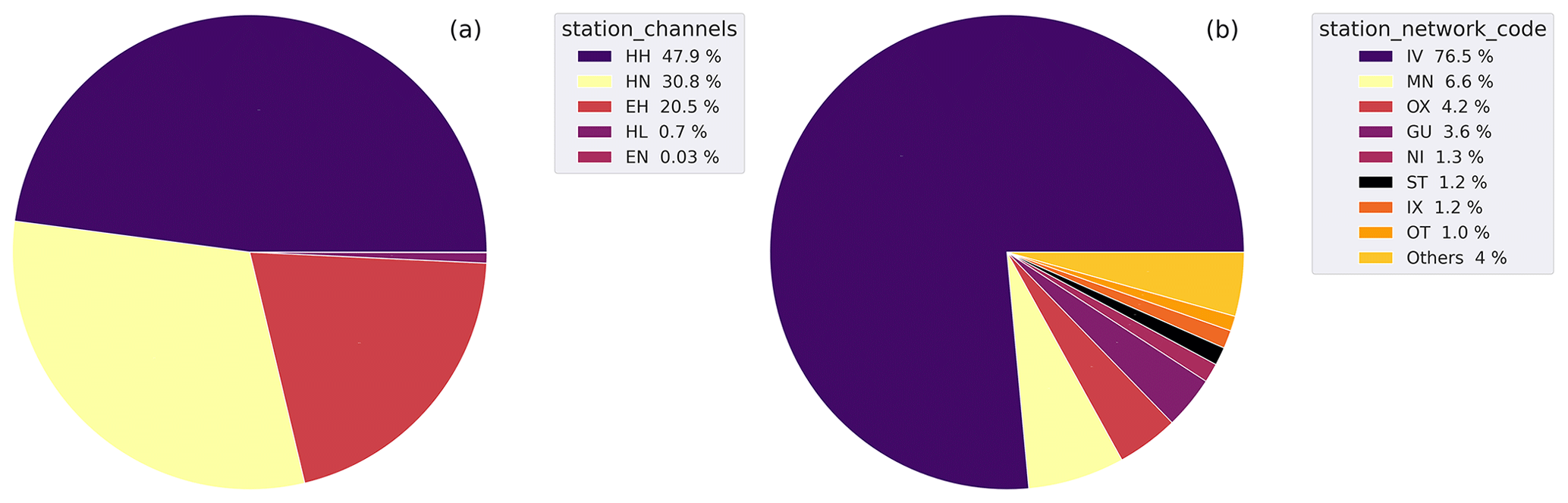
Figure 17Pie diagrams summarizing the distribution of the channels (a) and the data contributing networks (b) of the noise dataset.
The full list of station_network_code with %<1 collected in “Others” in decreasing order is SI, YD, 3A, XO, ZM, BA, AC, HL, TV, and RF.
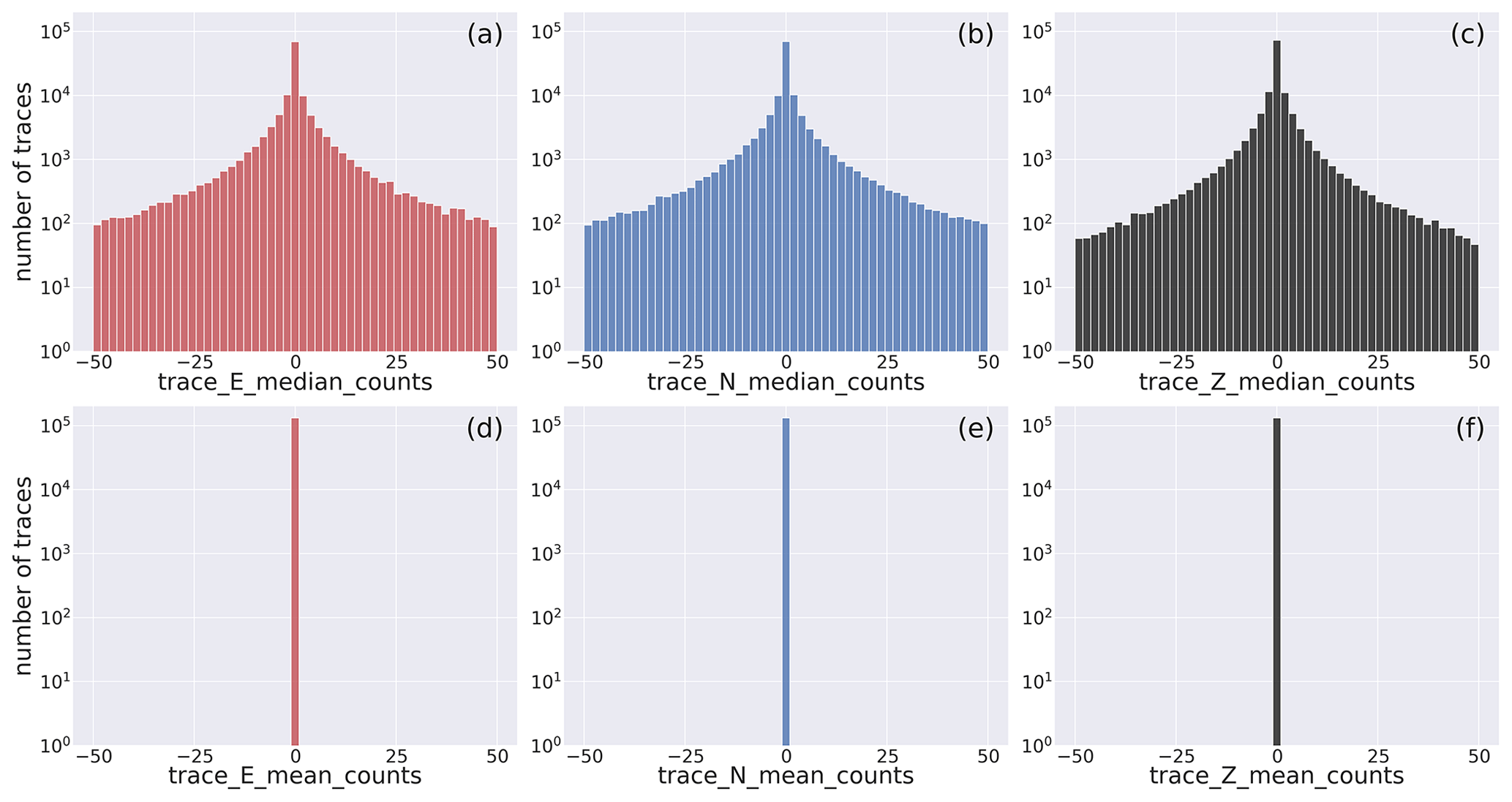
Figure 18Close view of the histogram of the distribution of the median and mean values of the E-, N-, and Z-component noise waveform traces. The full distribution is shown in Fig. D5. Note that the mean values (d–f) are shown to the sole scope of reference. The metadata names listed in Table 2 are used as labels for the specific metadata being represented.
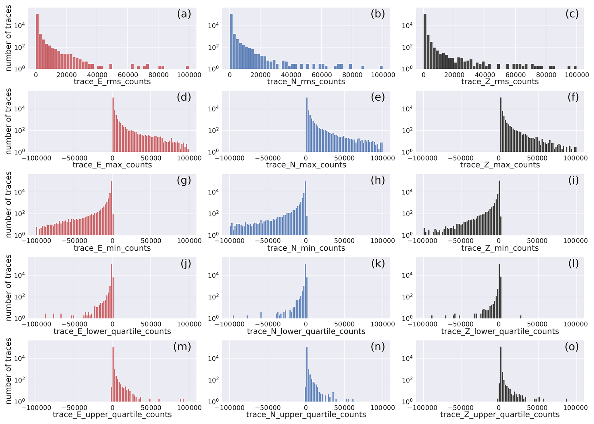
Figure 19Histogram of the distribution of the quality control metadata of the noise E-, N-, and Z-component waveform traces: rms, min, max, and first and third quartile. The width of the bins is 2×10³. The full distribution of values is provided in Fig. D6. The horizontal axis labels correspond to the metadata being represented which are listed in Table 2.
3.3 Examples of noise data traces
Examples of the noise traces are shown in Fig. 20. To perform the selection, we have used the distribution of the trace rms values that is provided in Table 5.
Table 5Distribution according to different quantiles of selected noise metadata (cf. Table 2) for the HH and EH channels.
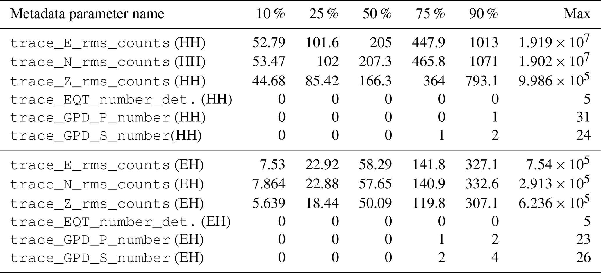
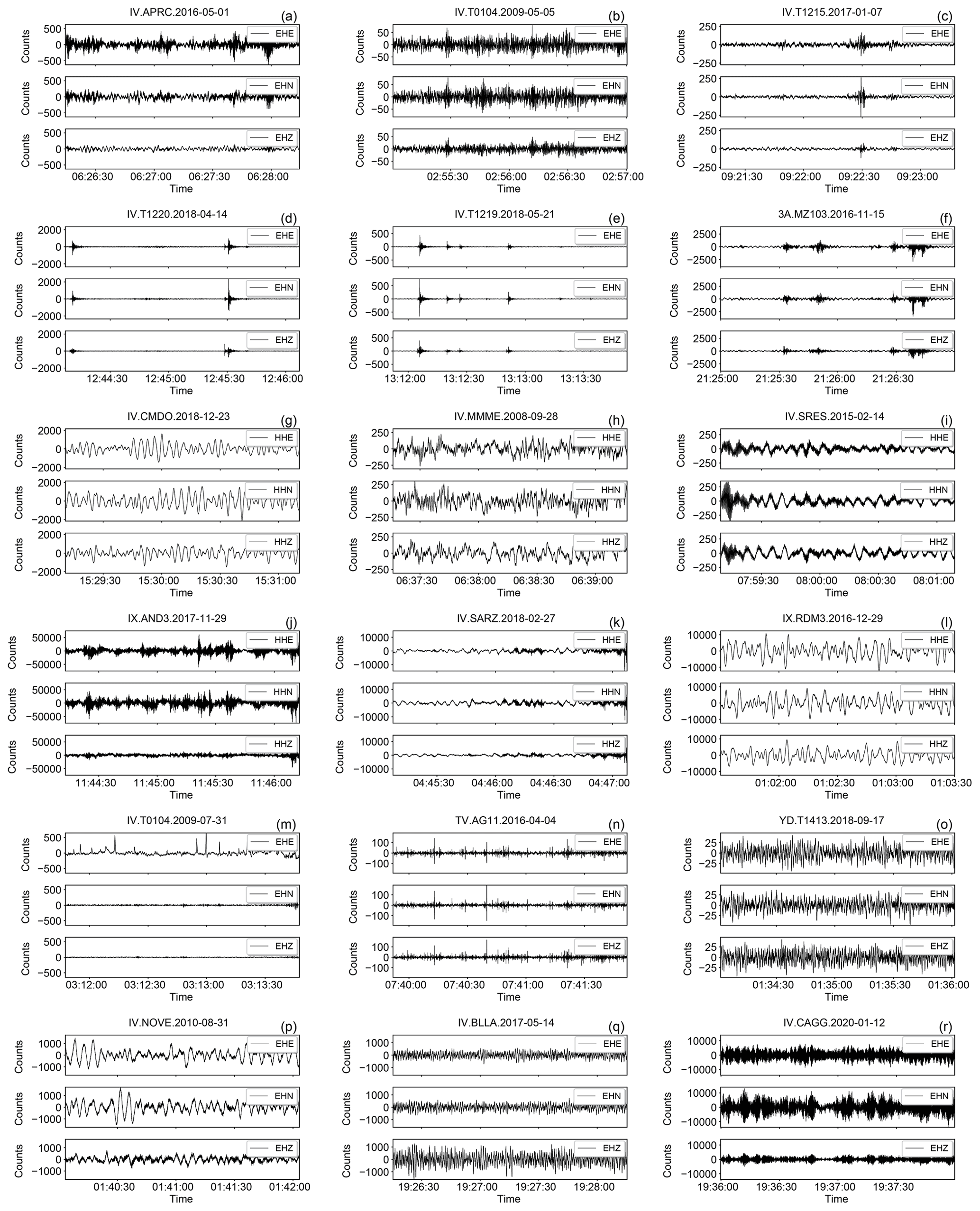
Figure 20Example of randomly selected noise waveforms of the HH and EH channels contained in INSTANCE. The traces are drawn randomly according to different criteria based on the metadata provided in Table 2 and on the quantile values listed in Table 5.
Each row contains three, randomly selected, 3C traces drawn according to the following criteria:
(a–c) trace_GPD_[P,S]_number >3 (11.6 % of the total of the EH channels);
(d–f) trace_EQT_number_detections >3 (0.13 % of the total of the EH channels);
(g–i) all the trace_[E,N,Z]_rms_counts < [1013, 1071, 793] (86.31 % of the total of the HH channels);
(j–l) any of the trace_[E,N,Z]_rms_counts > [1013, 1071, 793] (13.69 % of the total of the HH channels);
(m–o) all the trace_[E,N,Z]_rms_counts < [327.1, 332, 307] (86.36 % of the total of the EH channels);
(p–r) any of the trace_[E,N,Z]_rms_counts > [327.1, 332, 307] (13.64 % of the total of the EH channels).
In the top two rows of Fig. 20, some examples of events detected using the GPD and EQTransformer algorithms on the EH channels are shown. As it was the case with the event dataset, the noise traces also contain undetected events although their number according to our analysis seems rather small especially for the earthquakes detected by EQTransformer. This result gives us good confidence that the noise traces are for the great majority free of earthquake events. The following rows of Fig. 20 provide waveform samples drawn from the 90 % of the dataset (panels g–i and m–o) for the HH and EH channels, respectively. Both sets of panels exemplify some of the features of the great majority of the noise data. In contrast, the panels j–l and p–r have been chosen to show what could be considered traces exceeding noise values or that contain finite-duration events of uncertain origin.
The primary objective of this work has been to assemble a benchmark dataset consisting of seismic waveforms and associated metadata. It has been designed to be used for the analysis of earthquakes in Italy (and neighboring areas) using ML techniques, and it could prove useful for ML analysis also elsewhere in other active tectonic regions by adopting transfer learning methodologies (Jozinović et al., 2021). The dataset consists of three HDF5 volumes – raw and instrument removed event traces, as well as raw noise traces – and of the associated metadata.
The selection of the waveform traces to be included was based on the availability of low (≤1 s) P- and S-phase location residual times and large location weights taken from the preferred solutions listed in the INGV bulletin. To counteract the Gutenberg–Richter power law which affects the compilation of seismological datasets targeting ML analysis applications, attention was paid towards assembling a dataset that was not completely skewed by a large number of small-magnitude earthquakes. To this end, we included all the traces available of the larger-size earthquakes, and then we decreased progressively the number of smaller-size earthquakes and associated traces. Our effort, however, trades off with the need of assembling a dataset that is sufficiently large for ML purposes. The distribution of the selected traces shown in Figs. 3 and 4 according to magnitude, distance, and focal depth allows the users to make the appropriate choices for their purposes even though we recognize that the achievement of the sought balanced distribution remains difficult. Other data selection criteria could have been used (e.g., select all the data acquired within distance ranges depending on earthquake magnitude), but the (un)balanced magnitude and distance distribution would have persisted. Thus, given the criteria adopted it is pleonastic to remark that this dataset is not designed for studies addressing the earthquake magnitude power-law distribution (e.g., the b-value parameter). Similarly, although the dataset contains an average of 21 traces per earthquake, it may not be optimal for dedicated earthquake relocation studies.
Our criterion, based on the available high-quality P and S phases with low location residual times, is expected to provide a large number of traces with distinct earthquake signal and high SNRs. The distribution of SNR values shown in Figs. 10 and 11 and in Table 3 and the example seismograms shown in Figs. 14j–r and 15m–o appear to confirm our choices.
The selection of 120 s trace length time window is longer than those made by other authors for analogous benchmark datasets (e.g., Mousavi et al., 2019; Magrini et al., 2020). This relatively long time window was required, however, because we sought to include the entire seismicity occurring in Italy that spans from very shallow to very deep (Fig. 3). Unfortunately, this long window trades off with a higher probability of including earthquakes close in time that had not been reported in the INGV catalogue. For this reason, we carried out also a (preliminary) automatic picking and earthquake detection analysis using two well-established recent ML techniques (GPD and EQTransformer; Ross et al., 2018a; Mousavi et al., 2020) to possibly isolate those traces that include multiple events. The results of this analysis summarized in Table 3 would indicate that about 90 % of the event data contain only one earthquake according to the EQTransformer analysis, whereas the GPD analysis returned some slightly higher numbers of P- and S-phase detections.
Our metadata for the earthquake part of the dataset consist of 115 parameters. They are subdivided into three main classes plus one additional class derived from the previous ones. This is a rather rich set of parameters that can be used either (i) to select subsets of the dataset or (ii) as additional features to rely on when developing ML models, as labels in supervised ML analysis, or for unsupervised ML applications. In addition, the metadata could be used by themselves for specific studies (seismic velocity model regionalization, traveltime tomography, ground motion prediction models, local site corrections, etc.).
Earthquake data gathered by seismic instruments and streamed in real time to earthquake monitoring centers or preserved within archives can suffer from problems of different nature (e.g., sensor, data logger, equipment installation, data transmission, and processing among the most common). Thus, the compiled dataset could be useful for the development of robust techniques of analysis, and this is one main reason for including several trace quality parameters as metadata since they can help the user to identify the possibly faulty records, which can be then either removed or included to train the ML model just to “learn” them. This approach may seem to contradict one of the main purposes of compiling a high-quality dataset, and it may also be an obstacle when attempting to reveal deep information therein, but the expectation is that, by including all the data together, the rich set of metadata leaves the users enough freedom to identify the “good” data for their purposes. It is worthwhile to mention that Yeck et al. (2020) have found that inclusion of only good, high-SNR trace data during training of various body waves resulted in lower performance when applied to real-time pick data.
The INSTANCE dataset includes intensity measures (i.e., PGA, PGV, spectral accelerations) obtained after deconvolution of the instrument response performed automatically and possibly affected by digital signal processing problems induced, for example, by the presence of abnormal drifts and spikes. Given the difficulty in verifying the quality of all the individual processed traces, the availability of a rich set of trace metadata can be useful (again) to detect the faulty traces.
The example traces drawn randomly from the dataset that we have presented in Figs. 14, 15, 16, and 20 provide some evidence of the characteristics of the traces contained in the dataset and how they can be promptly selected through the provided metadata. Although the great majority of the data appear to be of very good quality, we are also aware that low-quality data almost inevitably occur. Inspection of the waveform traces by using other selection criteria than those shown here and of the IM metadata (see Fig. 12) gives us, however, good confidence on an overall good quality of the dataset.
The INSTANCE data collection assembles for the first time a very large amount of earthquake and noise data throughout Italy. If on one hand this might seem a limitation when compared to other recent data collections like STEAD and LEN-DB that have gathered data globally, on the other hand the dataset can be considered a representative subset of the seismicity in Italy and neighboring areas. The dataset equals to more than 43 000 h of continuous event and noise data and associated metadata with an average of 21 3C traces per earthquake. For the purpose of comparison, in Table 6, we summarize the main features of the currently available seismological datasets assembled for ML analysis. As noted above, the main features that distinguish INSTANCE from the other datasets are the number of metadata for both earthquakes and noise traces and the average number of traces per event. In addition, the dataset provides a generally large number of traces for each recording site, making the dataset suitable for quite diversified target studies. The dataset is also unique since it is the only one (yet) to provide the waveform traces in both digital counts and physical units. In this context, the set of parameters provided by INSTANCE spans both specific seismological parameters like P and S arrival times, fault plane and moment tensor solutions, and also peak ground motion parameters in physical units (e.g., PGA, PGV), which can be used for studies that target the estimation of the ground shaking (e.g., shakemaps).
Table 6Comparison between INSTANCE and other published seismic waveform datasets. It was not possible to retrieve some attributes of the original SCEDC dataset since it is available as different subsets extracted for specific application (list available at https://scedc.caltech.edu/data/deeplearing.html, last access: 19 November 2021).
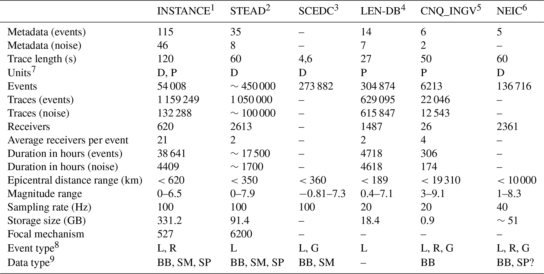
1 INSTANCE, https://doi.org/10.13127/instance. 2 STEAD, https://doi.org/10.1109/ACCESS.2019.2947848. 3 SCEDC, https://scedc.caltech.edu/data/deeplearning.html (last access: 19 November 2021). 4 LEN-DB, https://doi.org/10.5281/zenodo.3648232. 5 ConvNetQuake_INGV (CNQ_INGV), https://doi.org/10.5281/zenodo.5040865. 6 NEIC, https://doi.org/10.5066/P9OHF4WL. 7 D: digital; P: physical. 8 L: local; R: regional; G: global. 9 BB: broadband; SM: strong motion; SP: short period.
In summary, the dataset features strengths such as the prompt availability of a large number of records assembled within a ready-to-use data volume that can be certainly considered representative of the whole waveform data archive of the INGV ORFEUS-EIDA node and that can be used for many diverse studies. In our opinion, the strengths of providing a diversified set of data outnumber the weaknesses, and the latter ones be isolated and their negative contribution reduced through the exploitation of the very rich set of metadata.
For the purpose of describing the range of possible applications of INSTANCE, we follow the basic exposition schema adopted by Mousavi et al. (2019) for the STEAD benchmark dataset. These authors addressed four main areas in which benchmark datasets can prove very effective for improving seismological knowledge and seismic monitoring operational activities: earthquake trace denoising, earthquake detection and onset picking, classification/discrimination, and direct earthquake characterization.
The seismic noise level at a station is frequency dependent and derives from many factors such as types of equipment, installation, meteorological conditions, anthropic generated noise, geography, season, and time of day (McNamara and Buland, 2004). Seismic trace denoising enhances the SNR that is crucial to lowering the magnitude detection level of earthquake catalogs and, by so doing, increase the number events detected. Analogously, denoising can be relevant to preprocess seismic traces when performing ambient noise cross-correlation analysis (e.g., Baig et al., 2009), for detecting speed-of-light changes of the gravitational field (Vallée et al., 2017), or for the analysis of seismic data acquired in urban areas (e.g., Parolai, 2009), just to mention a few among many applications. ML techniques seem very promising to address the reduction of noise in seismic data. For example, W. Zhu et al. (2019) (and references therein for a list of applications in applied geophysics and seismology) have proposed a denoising/decomposition method, DeepDenoiser, based on a deep neural network which is based on the adoption of signal and noise masks which are then used to effectively decompose the input data into a signal of interest and noise. The technique has been tested against a dataset composed of broadband recordings of the North California Seismic Network which is similar to the data of INSTANCE. The adoption of an unsupervised machine learning method has been instead advocated by Chen et al. (2019), who have proposed it in combination with an autoencoder algorithm that adaptively learns the features from the raw noisy seismological datasets and uses the sparse constraint to suppress the learned trivial features that may be associated with the partial noise component. They apply the technique to the waveform stacked data used in Shearer (1991), and similar stacks can be promptly prepared using INSTANCE at the local/regional scale and applying the denoising technique accordingly.
Earthquake detection (including phase picking), discrimination, and rapid characterization represent main pillars of seismic monitoring and surveillance. During their lifetime, operational seismic centers alternate between calm periods characterized by low levels of seismicity, in which the detection of even the smallest possible events can become of relevance to delineate the activation of often hidden tectonic structures, and paroxysmal periods starting with significant earthquakes and followed by hundreds or thousands of aftershocks felt by people. To ameliorate the response of the centers in both these extreme cases, we find that the INSTANCE dataset can be of importance to calibrate and benchmark methodologies (i) for phase onset picking and earthquake detection methods to lower the magnitude detection level (e.g., Ross et al., 2018a; L. Zhu et al., 2019; Walter et al., 2020; Mousavi et al., 2020, among others); (ii) to discriminate between volcanic and tectonic earthquakes (e.g., Esposito et al., 2006) and, in the future, after updating INSTANCE with new data, discriminate between earthquakes and other sources of seismic energy (e.g., sonic booms, quarry blasts, underwater explosions) often felt by the population (e.g., Del Pezzo et al., 2003; Linville et al., 2019); (iii) for the rapid and accurate characterization of the earthquake source, distance, and depth (e.g., Perol et al., 2018; Trugman and Shearer, 2018; Kriegerowski et al., 2018; Zhang et al., 2020; Lomax et al., 2019; Mousavi and Beroza, 2020; Münchmeyer et al., 2021) and of the ground shaking (e.g., Alavi, 2011; Derras et al., 2012; Derras, 2014; Jozinović et al., 2020; Münchmeyer et al., 2020).
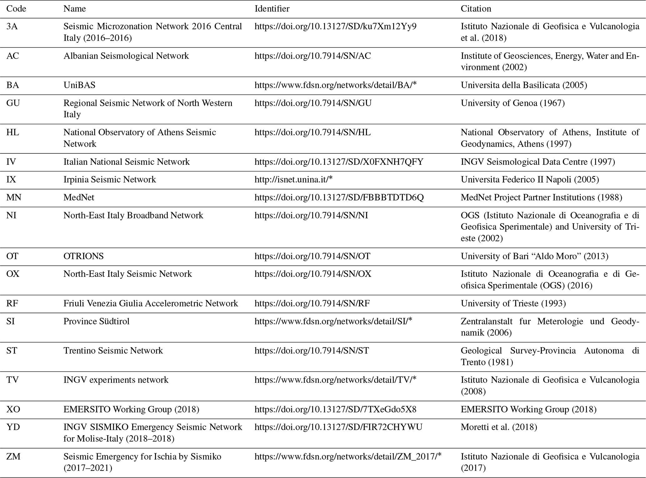
Istituto Nazionale di Geofisica e Vulcanologia et al. (2018)Institute of Geosciences, Energy, Water and Environment (2002)Universita della Basilicata (2005)University of Genoa (1967)National Observatory of Athens, Institute of Geodynamics, Athens (1997)INGV Seismological Data Centre (1997)Universita Federico II Napoli (2005)MedNet Project Partner Institutions (1988)OGS (Istituto Nazionale di Oceanografia e di Geofisica Sperimentale) and University of Trieste (2002)University of Bari “Aldo Moro” (2013)Istituto Nazionale di Oceanografia e di Geofisica Sperimentale (OGS) (2016)University of Trieste (1993)Zentralanstalt fur Meterologie und Geodynamik (2006)Geological Survey-Provincia Autonoma di Trento (1981)Istituto Nazionale di Geofisica e Vulcanologia (2008)EMERSITO Working Group (2018)Moretti et al. (2018)Istituto Nazionale di Geofisica e Vulcanologia (2017)Table 7Seismic networks used in the compilation of the INSTANCE dataset.
* last access: 19 November 2021.
Indeed, the field of application of the dataset is quite extensive, it can be used to address many diverse topics depending on how the data are grouped, and it can also be useful for applications not relying on ML techniques. For example, the dataset features some stations with several thousand traces recording earthquakes from different azimuths and distances that can be used to construct common-station gathers of seismograms for swaths of sources in almost any desired geometry (e.g., Korneev et al., 2003) or to study in detail the local site response. Analogously, the metadata alone provide a rich set of arrival times (cf. Fig. 7) that could be used as is for traveltime tomography at a regional scale in Italy, and, in addition, the availability of the associated waveforms makes possible the application of methodologies that resolve the velocity structure jointly using arrival times and waveform data (e.g., Zhang and Chen, 2014). For what concerns the ground motion amplitude data, the availability of these metadata can be of relevance in combination with the shakemaps to develop new tools for rapid earthquake ground motion estimation. Other applications of the data collection include the adoption of unsupervised ML algorithms to group the waveforms independently of the earthquake location and just on the waveform themselves (e.g., Seydoux et al., 2020). INSTANCE can also be used, as a dataset with a large number of data, for creating pretrained models when using transfer learning techniques either for seismological or other applications which use time-series data (Otović et al., 2021).
Overall, we believe that the dataset will be useful for stepping up towards a new generation of earthquake monitoring tools that will profit from the ongoing very fast developments in machine learning. What is certain is that seismology is in great need of benchmark datasets (Mousavi et al., 2019) upon which to test new and existing techniques. To this end, standardization of the input data and metadata formats is of great relevance, and in constructing this dataset we have adopted the schema proposed by the SeisBench initiative (Wollam et al., 2021). It is needless to emphasize that widespread adoption of the same metadata schema and data volume formats can foster the compilation of similar datasets also for other regions with the possibility of merging them all together giving the opportunity to perform ML analysis exploiting the potentials of the resulting large datasets. Perhaps more importantly, standardization of data and metadata formats will make it easier to test different datasets using the same ML model or, alternatively, benchmarking different models on the same dataset, and in both cases the benefits appear clear.
The data used in this work are all gathered on the Italian node of the European Integrated Data Archives (EIDA; http://eida.ingv.it/en/, last access: 19 November 2021) and were downloaded using the web services provided by INGV (http://terremoti.ingv.it/en/webservices_and_software, last access: 19 November 2021). The networks used for the INSTANCE dataset are organized in Table 7.
Routines and notebooks for analysis and display of the dataset (and the sample dataset) are available at https://github.com/ingv/instance (last access: 19 November 2021). The processing was performed using ObsPy (Beyreuther et al., 2010; Megies et al., 2011; Krischer et al., 2015), NumPy (Harris et al., 2020), SciPy (Virtanen et al., 2020), and Pandas (McKinney, 2010; The pandas development team, 2020) python modules, and the graphics were prepared using the Matplotlib library (Hunter, 2007) and seaborn (Waskom, 2021).
The dataset can be downloaded from http://doi.org/10.13127/instance (Michelini et al., 2021). A versioning schema has also been included since the dataset is expected to undergo modifications or expansions in the future. For instance, it is possible that some earthquakes or noise traces have been misclassified or that future significant seismic events have been included. A sample dataset is also provided on the same landing page.
INSTANCE is the first dataset designed for the application of ML methodologies compiled using the seismic data archived on the ORFEUS-EIDA node of INGV for Italy (Danecek et al., 2021). One of the main scopes of the dataset is to provide a benchmark for developing improved techniques for earthquake and ground motion characterization. The dataset consists of about 1.3 million, 120 s long each, 100 Hz sampling, 3C traces subdivided into about 1.2 million containing seismic events and more than 100 000 that include noise. The traces are assembled within HDF5 formatted volumes to facilitate access and analysis. More than 100 metadata grouped according to source, station, and trace (and derived quantities) are associated with each trace to give the user much flexibility and control for the selection of the most appropriate data for her/his scientific targets.
The event data include recordings of earthquakes in the magnitude range and in the distance range between 0 and more than 600 km, although the great majority of the traces belong to earthquakes in the magnitude range and within 250 km. The depth of the earthquakes varies between very shallow crustal earthquakes and about 600 km depth in the Calabrian subduction slab. The data have been recorded by more than 600 stations operating in Italy in the time span January 2005–January 2020. The dataset equals to more than 43 000 h of continuous event and noise data and associated metadata. An average of 21 3C traces is provided per earthquake.
The waveform trace data are provided in binary HDF5 file volumes. The volumes have been prepared for event data in counts and ground motion units and for noise data in counts.
The HDF5 format allows for rapid and easy access to the individual traces without the need of loading the whole dataset into memory.
The waveform trace datasets have been created using the HDF5 group data structure https://portal.hdfgroup.org/display/HDF5/HDF5 (last access: 19 November 2021), which contains as many HDF5 datasets as 3C waveforms.
Every three-component waveform is a separate HDF5 dataset and is accessed by its trace name (trace_name), found in the metadata file.
The earthquake locations provided in the Italian Seismic Bulletin (http://terremoti.ingv.it/en/help#BSI, last access: 19 November 2021) are fully described by Mele et al. (2010). The model consists of two layers over a half space assuming a ratio .
Table B1P- and S-wave velocity model used in the location procedures for the Italian Seismic Bulletin.

The IPOP software developed by Alberto Basili is used for the earthquake locations (Bono, 2008).
In this Appendix, we examine the origin for the observed asymmetry (almost 2:1 ratio) in the number of reported positive (up) and negative (down) polarities of the INSTANCE dataset. We evaluate whether (i) the inclusion of anthropic, unidentified sources like quarry blasts mistaken for earthquakes can affect the reported asymmetry and (ii) the tectonics of the region can condition the number of positive and negative polarities in INSTANCE.
For the first investigation, we have followed Mele et al. (2010) (see also the recent work by Gulia and Gasperini, 2021), who found that in the 2008 bulletin 99.6 % of the blasts have local magnitude ML≤2.2 (Fig. 23 of their study). We have progressively increased the lower magnitude threshold to verify whether the nearly 2:1 ratio between positive and negative polarities persists as the magnitude is increased. The expectation is that, as the magnitude increases, the ratio progressively levels out since the blasts (or other artificial sources) do not produce magnitudes greater than M=3 in Europe (cf. Giardini et al., 2004). To address the variation of the proportion between positive and negative polarities with magnitude, we have selected from the INSTANCE dataset earthquakes with progressively larger minimum threshold magnitudes and found that the fraction (percent values) of negative polarities increases progressively from 36 % to 41 % when including earthquakes with M>0.25 and M>3, respectively. For larger minimum magnitudes, the percentage stabilizes around 42 %–43 %. This indicates that inclusion of the polarities of, e.g., unrecognized blasts (i.e., with M<3) has a moderate but still significant impact on the observed asymmetry between the reported positive and negative polarities. This asymmetry, although somewhat surprising, seems to occur also elsewhere. For example, Ross et al. (2018b) report, in their analysis of the southern California earthquake dataset (before data augmentation), a content of 67 % and 33 % for up and down polarities, respectively. We also note that the regional tectonic setting in Southern California is quite different from that in Italy.
Secondly, we have subdivided the Italian area into two zones selecting earthquakes with magnitude M>2.5 occurring in the Apennines (defined as a rectangular area from 41 to 44∘ N latitude and 9 to 15∘ E longitude) and elsewhere outside this area. This data selection is aimed at verifying if the observed asymmetry of positive and negative polarities can result from the dominant extensional stress field characterizing the Apennines when compared to the other areas in Italy. In the Apennine target area, the largest majority of the earthquakes are characterized by normal faulting mechanisms: in this case the lobes of the seismic radiation pattern show negative polarities at short epicentral distances.
Given these conditions, the observed asymmetry could result from the complex interplay between the source receiver geometry, the 200–300 km width of peninsular Italy, and the dominant NE–SW extensional axis direction characterizing the tectonic regime in the Apennines. In this setting, the radiation pattern predicts negative polarities in the near field and positive polarities farther away from the source. Also the negative lobes are characterized by a smaller extension with respect to the positive lobes. Since the seismic receivers are more or less evenly distributed, the chance to record a negative pulse is smaller with respect to the positive one.
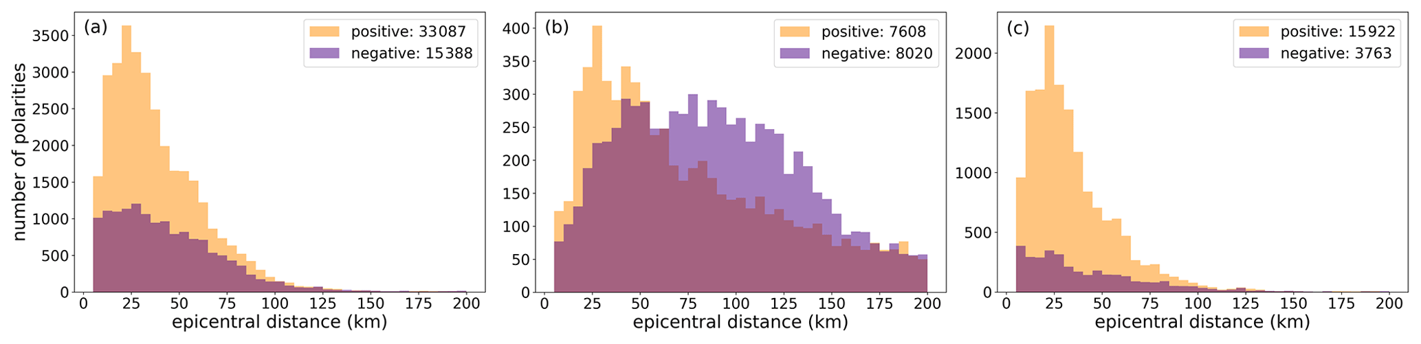
Figure C1Distribution of the positive and negative P-wave polarities for earthquakes with M>2.5 in the Apennine region (41–44∘ N and 9–15∘ E) (a); (b) as in panel (a) but for earthquakes outside the Apennines; (c) as in panel (a) but filtered by back azimuth along the NE–SW directions, corresponding to the intervals 15–105∘ and 195–285∘.
The Fig. C1 shows the histograms of the distribution of the positive and negative polarities with distance. The Fig. C1a shows the distribution of the polarities for the chosen target area in the Apennines, while Fig. C1c exhibits the polarities in the same area but only along back azimuth approximately NE–SW (i.e., the ranges 15–105∘ and 195–285∘). Finally, Fig. C1b displays the polarities from earthquakes outside the target area. We note that within the target area (Fig. C1a) the polarities are overwhelmingly positive, in gross agreement with the explanation above. For further confirmation, we note in Fig. C1c that, if we restrict to the NE–SW propagation direction perpendicular to the Italian Peninsula, the ratio between positive and negative polarities (positive %, negative %) increases further from (68 %, 32 %) to (81 %, 19 %), respectively. Conversely, the number of polarities for the earthquakes outside the target area are pretty much well balanced (49 %, 51 %) as shown in Fig. C1b.
In conclusion, (i) the INSTANCE dataset does contain positive polarities resulting from the inclusion of quarry blasts misidentified as earthquakes for magnitudes M≲2.5–3.0.
This follows from what reported by Mele et al. (2010)
(see also the recent work by Gulia and Gasperini, 2021)
and the change in positive and negative polarity proportions in INSTANCE at varying minimum magnitude thresholds appears to confirm it; (ii) the current modalities of earthquake revision at INGV do not allow for the identification of all the anthropic sources, so the (source_type) parameter of the metadata can be misleading; (iii) the target area in the selected Apennine region includes 76 % of the total number of polarities of the dataset and features a dominance of positive polarities: a possible explanation is the dominant normal type of earthquake faulting in the selected Apennine region; and (iv) the asymmetry observed in the target Apennine region disappears for M>2.5 elsewhere in Italy.
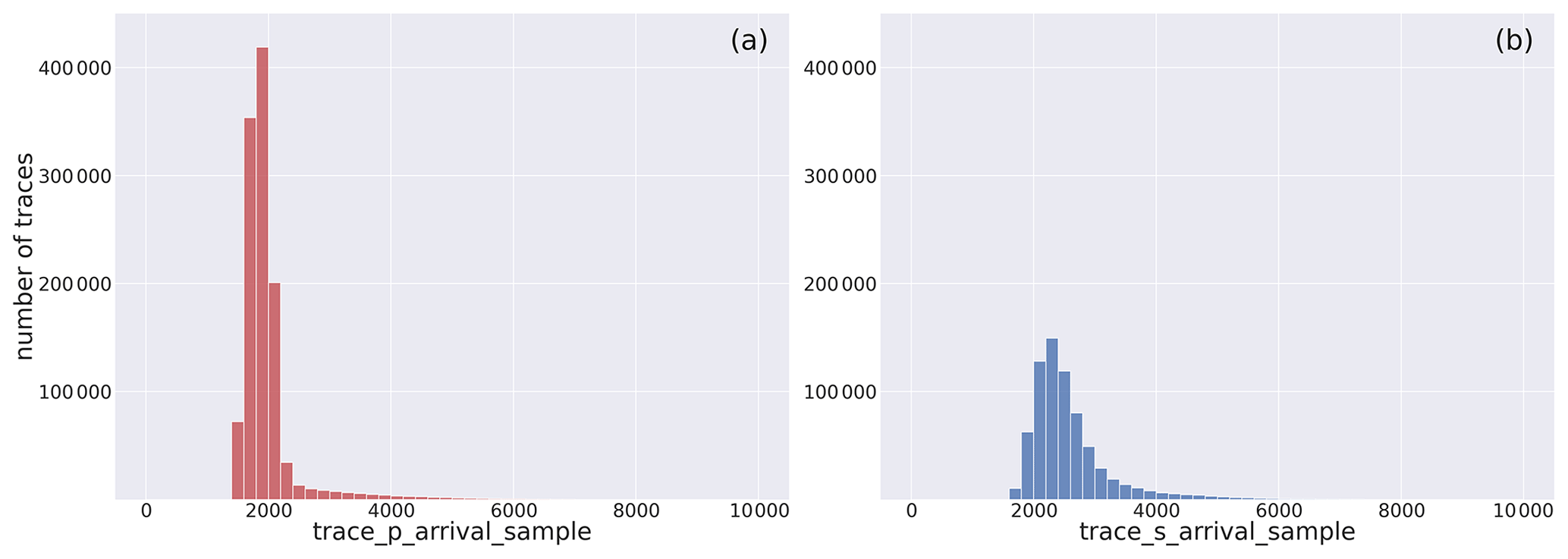
Figure D1Distribution of P- (a) and S-arrival (b) samples of the extracted waveform traces belonging to the earthquake dataset.
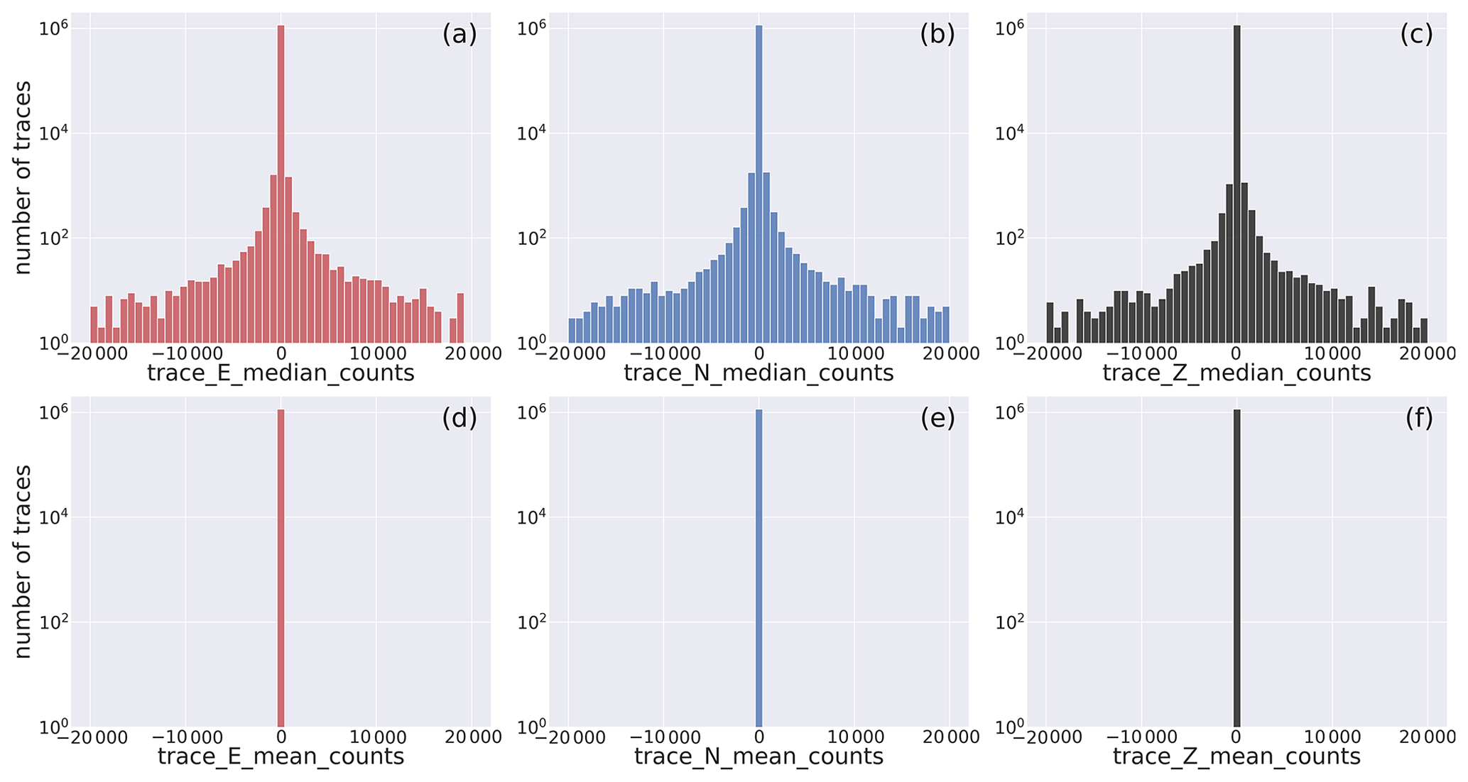
Figure D2Histogram of the distribution of the quality control metadata of the full earthquake dataset, with the horizontal axis inclusive of the complete range of values: median (a–c) and mean (d–f). The width of the bins is 2×10³; axes are labeled according to the metadata listed in Table 2.
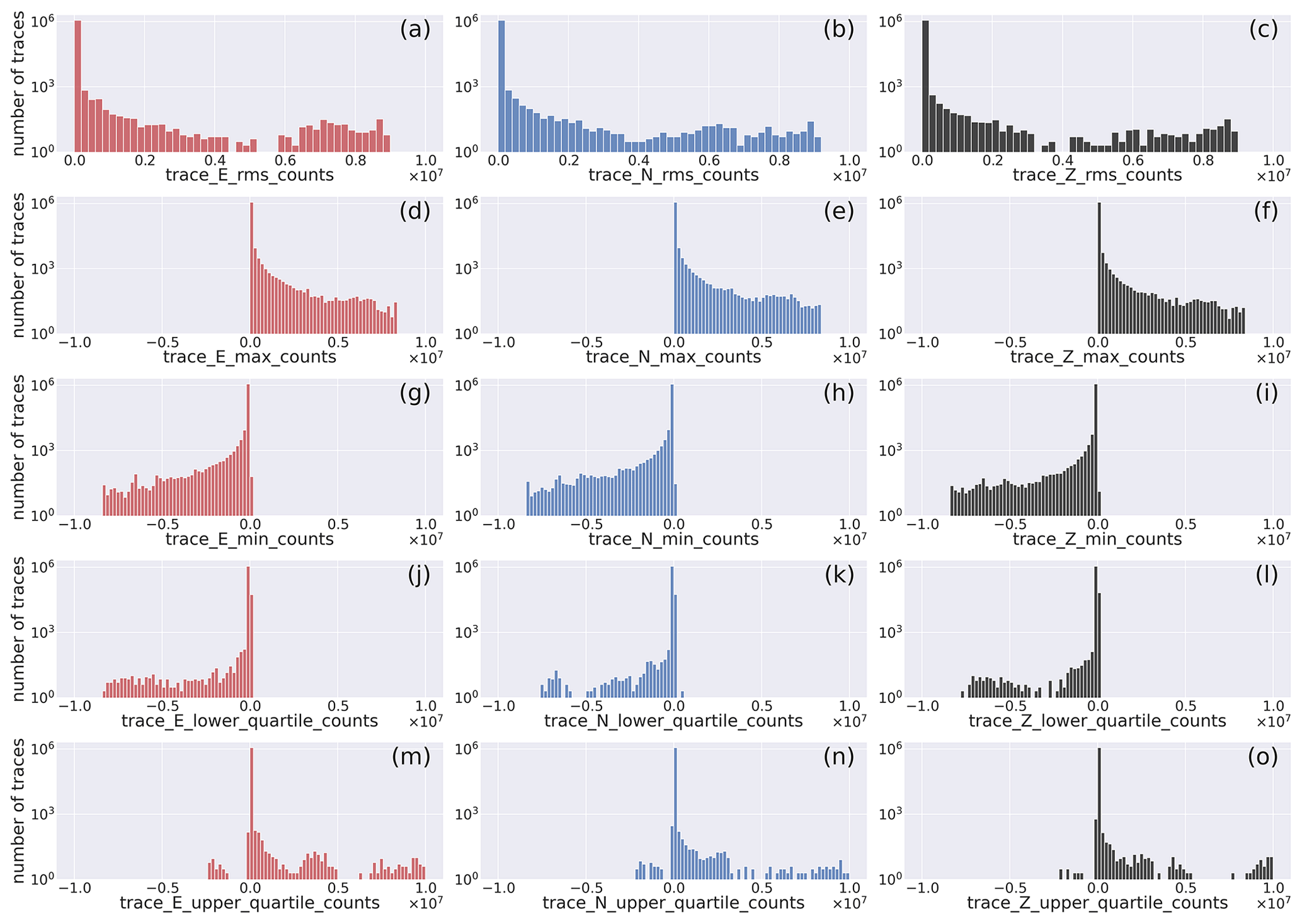
Figure D3Histogram of the distribution of quality control metadata of the full earthquake dataset, with the horizontal axis inclusive of the complete range of values: rms, min, max, and first and third quartile. The width of the bins is 2×10⁵; axes are labeled according to the metadata listed in Table 2.

Figure D4Histograms of the distribution of the intensity measures (IMs) of the earthquake dataset for M≥2 earthquakes, with the horizontal axis inclusive of the complete range of values. Axes are labeled according to the metadata listed in Table 2.

Figure D5Histogram of the distribution of the noise quality control metadata including the full range of values attained by the median values: median (a–c) and mean (d–f). The width of the bins is 2×10³; axes are labeled according to the metadata listed in Table 2.

AM prepared the initial data and metadata selection, drafted the manuscript, and created the initial version of the figures. SC and SG provided ML estimation of the waveform data and contributed to final versions of the figures and manuscript revision. CG contributed to data preparation and manuscript revision. DJ compiled the HDF5 formatted volumes and contributed to the data and manuscript revision. VL set up the virtual machines and the scripts to perform the massive data download.
The contact author has declared that neither they nor their co-authors have any competing interests.
The authors decline any responsibility for possible errors present in the INSTANCE dataset which can lead erroneous evaluations and to physical and economic damages.
Publisher's note: Copernicus Publications remains neutral with regard to jurisdictional claims in published maps and institutional affiliations.
This work would not have been possible without the effort and dedication of the people that install and maintain the stations of the networks used here, as well as the skilled IT people that are in charge of archiving, curating, and providing access to the data. We also greatly acknowledge the earthquake analysts that routinely perform the data analysis for the compilation of the earthquake bulletins. The metadata nomenclature benefited from the interaction and discussions within the recently formed SeisBench group. Sonja Gaviano benefited from the DL training schools organized by the Cost Action 17137 G2NET, coordinated by Elena Cuoco, who is kindly acknowledged. We would like to thank Jannes Münchmeyer, Elisa Tinti, and Anthony Lomax for reading the initial manuscript and providing suggestions. The reviewers Martijn van den Ende and John Clinton are kindly acknowledged for the insightful comments, questions, and suggestions that helped to clarify the text and improve the manuscript overall.
This work has been partially supported by the project INGV Pianeta Dinamico 2021 Tema 8 SOME (grant no. CUP D53J1900017001) funded by the Italian Ministry of University and Research “Fondo finalizzato al rilancio degli investimenti delle amministrazioni centrali dello Stato e allo sviluppo del Paese, legge 145/2018” and by the European Union's Horizon 2020 research and innovation program (grant no. 821115), Real-time Earthquake Risk Reduction for a Resilient Europe (RISE).
This paper was edited by Kirsten Elger and reviewed by John Clinton and Martijn van den Ende.
Abadi, M., Agarwal, A., Barham, P., Brevdo, E., Chen, Z., Citro, C., Corrado, G. S., Davis, A., Dean, J., Devin, M., Ghemawat, S., Goodfellow, I., Harp, A., Irving, G., Isard, M., Jia, Y., Jozefowicz, R., Kaiser, L., Kudlur, M., Levenberg, J., Mane, D., Monga, R., Moore, S., Murray, D., Olah, C., Schuster, M., Shlens, J., Steiner, B., Sutskever, I., Talwar, K., Tucker, P., Vanhoucke, V., Vasudevan, V., Viegas, F., Vinyals, O., Warden, P., Wattenberg, M., Wicke, M., Yu, Y., and Zheng, X.: TensorFlow: Large-Scale Machine Learning on Heterogeneous Distributed Systems, arXiv [preprint], arXiv:1603.04467, 14 March 2016. a
Alavi, A. H.: Prediction of principal ground-motion parameters using a hybrid method coupling artificial neural networks and simulated annealing, Comput. Struct., 89, 2176–2194, https://doi.org/10.1016/j.compstruc.2011.08.019, 2011. a
Baig, A. M., Campillo, M., and Brenguier, F.: Denoising seismic noise cross correlations, J. Geophys. Res., 114, B08310, https://doi.org/10.1029/2008JB006085, 2009. a
Bergen, K. J., Johnson, P. A., de Hoop, M. V., and Beroza, G. C.: Machine learning for data-driven discovery in solid Earth geoscience, Science, 363, eaau0323, https://doi.org/10.1126/science.aau0323, 2019. a
Beyreuther, M., Barsch, R., Krischer, L., Megies, T., Behr, Y., and Wassermann, J.: ObsPy: A Python Toolbox for Seismology, Seismol. Res. Lett., 81, 530–533, https://doi.org/10.1785/gssrl.81.3.530, 2010. a, b
Bono, A.: SisPick! 2.0 Sistema interattivo per l'interpretazione di segnali sismici, Manuale utente, Tech. Rep. Rapporti tecnici, n. 59, INGV, Rome, Italy, available at: http://editoria.rm.ingv.it/archivio_pdf/rapporti/58/pdf/rapporti_59.pdf (last access: 30 August 2021), 2008. a
Boore, D. M.: Estimating Vs(30) (or NEHRP Site Classes) from Shallow Velocity Models (Depths < 30 m), B. Seismol. Soc. Am., 94, 591–597, https://doi.org/10.1785/0120030105, 2004. a
Buland, R.: SEED Reference Manual, Tech. Rep., Incorporated Research Institutions for Seismology (IRIS), available at: http://www.fdsn.org/pdf/SEEDManual_V2.4.pdf (last access: 30 August 2021), 2006. a
Chen, Y., Zhang, M., Bai, M., and Chen, W.: Improving the Signal-to-Noise Ratio of Seismological Datasets by Unsupervised Machine Learning, Seismol. Res. Lett., 90, 1552–1564, https://doi.org/10.1785/0220190028, 2019. a
Chollet, F. and others: Keras [code], available at: https://keras.io (last access: 25 November 2021), 2015. a
Danecek, P., Pintore, S., Mazza, S., Mandiello, A., Fares, M., Carluccio, I., Della Bina, E., Franceschi, D., Moretti, M., Lauciani, V., Quintiliani, M., and Michelini, A.: The Italian Node of the European Integrated Data Archive, Seismol. Res. Lett., 92, 1726–1737, https://doi.org/10.1785/0220200409, 2021. a, b, c, d, e
Del Pezzo, E., Esposito, A., Giudicepietro, F., Marinaro, M., Martini, M., and Scarpetta, S.: Discrimination of Earthquakes and Underwater Explosions Using Neural Networks, B. Seismol. Soc. Am., 93, 215–223, https://doi.org/10.1785/0120020005, 2003. a
Derras, B.: Peak Ground Acceleration Prediction Using Artificial Neural Networks Approach: Application to the Kik-Net Data, International Journal of Earthquake Engineering and Hazard Mitigation, 2, 144–153, https://doi.org/10.15866/irehm.v2i4.7121, 2014. a
Derras, B., Bard, P., Cotton, F., and Bekkouche, A.: Adapting the Neural Network Approach to PGA Prediction: An Example Based on the KiK‐net Data, B. Seismol. Soc. Am., 102, 1446–1461, https://doi.org/10.1785/0120110088, 2012. a
Dramsch, J. S.: Chapter One – 70 years of machine learning in geoscience in review, Adv. Geophys., 61, 1–55, https://doi.org/10.1016/bs.agph.2020.08.002, 2020. a
EMERSITO Working Group: Rete sismica del gruppo EMERSITO, sequenza sismica del 2016 in Italia Centrale, Instituto Nazionale di Geofisica e Vulcanologia [data set], https://doi.org/10.13127/SD/7TXEGDO5X8, 2018. a
Esposito, A. M., Giudicepietro, F., Scarpetta, S., D'Auria, L., Marinaro, M., and Martini, M.: Automatic Discrimination among Landslide, Explosion-Quake, and Microtremor Seismic Signals at Stromboli Volcano Using Neural Networks, B. Seismol. Soc. Am., 96, 1230–1240, https://doi.org/10.1785/0120050097, 2006. a
Fang, L., Wu, Z., and Song, K.: SeismOlympics, Seismol. Res. Lett., 88, 1429–1430, https://doi.org/10.1785/0220170134, 2017. a
Geological Survey-Provincia Autonoma di Trento: Trentino Seismic Network, International Federation of Digital Seismograph Networks [data set], https://doi.org/10.7914/SN/ST, 1981. a
Giardini, D., Wiemer, S., Faeh, D., and Deichmann, N.: Seismic Hazard Assessment of Switzerland, 2004, Tech. Rep., Swiss Seismological Service, ETH Zurich, available at: http://www.seismo.ethz.ch/export/sites/sedsite/knowledge/.galleries/pdf_hazard2004/hazard_report_2004.pdf_2063069299.pdf (last access: 25 November 2021), 2004. a
Gulia, L. and Gasperini, P.: Contamination of Frequency–Magnitude Slope (b‐Value) by Quarry Blasts: An Example for Italy, Seismol. Res. Lett., 92, 3538–3551, https://doi.org/10.1785/0220210080, 2021. a, b
Gutenberg, B. and Richter, C. F.: Frequency of earthquakes in California, B. Seismol. Soc. Am., 34, 185–188, 1944. a
Harris, C. R., Millman, K. J., van der Walt, S. J., Gommers, R., Virtanen, P., Cournapeau, D., Wieser, E., Taylor, J., Berg, S., Smith, N. J., Kern, R., Picus, M., Hoyer, S., van Kerkwijk, M. H., Brett, M., Haldane, A., del Río, J. F., Wiebe, M., Peterson, P., Gérard-Marchant, P., Sheppard, K., Reddy, T., Weckesser, W., Abbasi, H., Gohlke, C., and Oliphant, T. E.: Array programming with NumPy, Nature, 585, 357–362, https://doi.org/10.1038/s41586-020-2649-2, 2020. a
Hunter, J. D.: Matplotlib: A 2D graphics environment, Comput. Sci. Eng., 9, 90–95, https://doi.org/10.1109/MCSE.2007.55, 2007. a, b
Ingate, S.: The IRIS Consortium: Community Based Facilities and Data Management for Seismology, in: Earthquake Monitoring and Seismic Hazard Mitigation in Balkan Countries, NATO Science Series: IV: Earth and Environmental Sciences, edited by: Husebye, E. S., vol. 81, 121–132, Springer, Dordrecht, https://doi.org/10.1007/978-1-4020-6815-7_8, 2008. a
INGV Seismological Data Centre: Rete Sismica Nazionale (RSN), Instituto Nazionale di Geofisica e Vulcanologia [data set], https://doi.org/10.13127/SD/X0FXNH7QFY, 1997. a
Institute of Geosciences, Energy, Water and Environment: Albanian Seismological Network, International Federation of Digital Seismograph Networks [data set], https://doi.org/10.7914/SN/AC, 2002. a
Istituto Nazionale di Geofisica e Vulcanologia (INGV): INGV experiments network, Instituto Nazionale di Geofisica e Vulcanologia [data set], available at: http://cnt.rm.ingv.it/instruments/network/TV (last access: 19 November 2021), 2008. a
Istituto Nazionale di Geofisica e Vulcanologia (INGV): Seismic Emergency for Ischia by Sismiko (2017–2021), International Federation of Digital Seismograph Networks [data set], available at: https://www.fdsn.org/networks/detail/ZM_2017/ (last access: 19 November 2021), 2017. a
Istituto Nazionale di Geofisica e Vulcanologia (INGV), Istituto di Geologia Ambientale e Geoingegneria (CNR-IGAG), Istituto per la Dinamica dei Processi Ambientali (CNR-IDPA), Istituto di Metodologie per l'Analisi Ambientale (CNR-IMAA), and Agenzia Nazionale per le nuove tecnologie, l’energia e lo sviluppo economico sostenibile (ENEA): Rete del Centro di Microzonazione Sismica (CentroMZ), sequenza sismica del 2016 in Italia Centrale, Instituto Nazionale di Geofisica e Vulcanologia [data set], https://doi.org/10.13127/SD/KU7XM12YY9, 2018. a
Istituto Nazionale di Oceanografia e di Geofisica Sperimentale (OGS): North-East Italy Seismic Network, International Federation of Digital Seismograph Networks [data set], https://doi.org/10.7914/SN/OX, 2016. a
Jia, Y., Shelhamer, E., Donahue, J., Karayev, S., Long, J., Girshick, R., Guadarrama, S., and Darrell, T.: Caffe: Convolutional Architecture for Fast Feature Embedding, arXiv [preprint], arXiv:1408.5093, 20 June 2014. a
Johnson, P. A., Rouet Leduc, B., Pyrak-Nolte, L. J., Beroza, G. C., Marone, C. J., Hulbert, C., Howard, A., Singer, P., Gordeev, D., Karaflos, D., Levinson, C. J., Pfeiffer, P., Puk, K. M., and Reade, W.: Laboratory earthquake forecasting: A machine learning competition, P. Natl. Acad. Sci. USA, 118, e2011362118, https://doi.org/10.1073/pnas.2011362118, 2021. a
Jozinović, D., Lomax, A., Štajduhar, I., and Michelini, A.: Rapid prediction of earthquake ground shaking intensity using raw waveform data and a convolutional neural network, Geophys. J. Int., 222, 1379–1389, https://doi.org/10.1093/gji/ggaa233, 2020. a, b, c
Jozinović, D., Lomax, A. J., Stajduhar, I., and Michelini, A.: SSA 2021 Annual Meeting, Seismol. Res. Lett., 92, 1213–1479, https://doi.org/10.1785/0220210025, 2021. a
Kong, Q., Trugman, D. T., Ross, Z. E., Bianco, M. J., Meade, B. J., and Gerstoft, P.: Machine Learning in Seismology: Turning Data into Insights, Seismol. Res. Lett., 90, 3–14, https://doi.org/10.1785/0220180259, 2018. a
Korneev, V. A., Nadeau, R. M., and McEvilly, T. V.: Seismological Studies at Parkfield IX: Fault-Zone Imaging Using Guided Wave Attenuation, B. Seismol. Soc. Am., 93, 1415–1426, https://doi.org/10.1785/0120020114, 2003. a
Kriegerowski, M., Petersen, G. M., Vasyura Bathke, H., and Ohrnberger, M.: A Deep Convolutional Neural Network for Localization of Clustered Earthquakes Based on Multistation Full Waveforms, Seismol. Res. Lett., 90, 510–516, https://doi.org/10.1785/0220180320, 2018. a
Krischer, L., Megies, T., Barsch, R., Beyreuther, M., Lecocq, T., Caudron, C., and Wassermann, J.: ObsPy: a bridge for seismology into the scientific Python ecosystem, Computational Science & Discovery, 8, 014003, https://doi.org/10.1088/1749-4699/8/1/014003, 2015. a, b
Lanzano, G., Luzi, L., Russo, E., Felicetta, C., D'Amico, M., Sgobba, S., and Pacor, F.: Engineering Strong Motion Database (ESM) flatfile [data set], Tech. Rep., Istituto Nazionale di Geofisica e Vulcanologia (INGV), https://doi.org/10.13127/esm/flatfile.1.0, 2018. a
Linville, L., Pankow, K., and Draelos, T.: Deep Learning Models Augment Analyst Decisions for Event Discrimination, Geophys. Res. Lett., 46, 3643–3651, https://doi.org/10.1029/2018GL081119, 2019. a
Lomax, A., Michelini, A., and Jozinović, D.: An Investigation of Rapid Earthquake Characterization Using Single‐Station Waveforms and a Convolutional Neural Network, Seismol. Res. Lett., 90, 517–529, https://doi.org/10.1785/0220180311, 2019. a
Magrini, F., Jozinovic, D., Cammarano, F., Michelini, A., and Boschi, L.: Local earthquakes detection: A benchmark dataset of 3-component seismograms built on a global scale, Artificial Intelligence in Geosciences, 1, 1–10, https://doi.org/10.1016/j.aiig.2020.04.001, 2020. a, b
Margheriti, L., Nostro, C., Cocina, O., Castellano, M., Moretti, M., Lauciani, V., Quintiliani, M., Bono, A., Mele, F. M., Pintore, S., Montalto, P., Peluso, R., Scarpato, G., Rao, S., Alparone, S., Di Prima, S., Orazi, M., Piersanti, A., Cecere, G., Cattaneo, M., Vicari, A., Sepe, V., Bignami, C., Valoroso, L., Aliotta, M., Azzarone, A., Baccheschi, P., Benincasa, A., Bernardi, F., Carluccio, I., Casarotti, E., Cassisi, C., Castello, B., Cirilli, F., D'Agostino, M., D'Ambrosio, C., Danecek, P., Cesare, W. D., Bina, E. D., Di Filippo, A., Di Stefano, R., Faenza, L., Falco, L., Fares, M., Ficeli, P., Latorre, D., Lorenzino, M. C., Mandiello, A., Marchetti, A., Mazza, S., Michelini, A., Nardi, A., Pastori, M., Pignone, M., Prestifilippo, M., Ricciolino, P., Sensale, G., Scognamiglio, L., Selvaggi, G., Torrisi, O., Zanolin, F., Amato, A., Bianco, F., Branca, S., Privitera, E., and Stramondo, S.: Seismic Surveillance and Earthquake Monitoring in Italy, Seismol. Res. Lett., 92, 1659–1671, https://doi.org/10.1785/0220200380, 2021. a
McKinney, W.: Data Structures for Statistical Computing in Python, in: Proceedings of the 9th Python in Science Conference, edited by: van der Walt, S. and Millman, J., pp. 56–61, https://doi.org/10.25080/Majora-92bf1922-00a, 2010. a
McNamara, D. E. and Buland, R. P.: Ambient Noise Levels in the Continental United States, B. Seismol. Soc. Am., 94, 1517–1527, https://doi.org/10.1785/012003001, 2004. a
MedNet Project Partner Institutions: Mediterranean Very Broadband Seismographic Network (MedNet), Instituto Nazionale di Geofisica e Vulcanologia [data set], https://doi.org/10.13127/SD/FBBBTDTD6Q, 1988. a
Megies, T., Beyreuther, M., Barsch, R., Krischer, L., and Wassermann, J.: ObsPy – What can it do for data centers and observatories?, Ann. Geophys.-Italy, 54, 47–58, https://doi.org/10.4401/ag-4838, 2011. a, b
Meier, M.-A., Ross, Z. E., Ramachandran, A., Balakrishna, A., Nair, S., Kundzicz, P., Li, Z., Andrews, J., Hauksson, E., and Yue, Y.: Reliable Real-Time Seismic Signal/Noise Discrimination With Machine Learning, J. Geophys. Res.-Sol. Ea., 124, 788–800, https://doi.org/10.1029/2018JB016661, 2019. a
Mele, F., Arcoraci, L., Battelli, P., Berardi, M., Castellano, C., Lozzi, G., Marchetti, A., Nardi, A., Pirro, M., and Rossi, A.: Bollettino Sismico Italiano 2008 (Italian Seismic Bulletin 2008), Quaderni di geofisica, p. 45, available at: https://istituto.ingv.it/images/collane-editoriali/quaderni-di-geofisica/quaderni-di-geofisica-2010/quaderno85.pdf (last access: 19 November 2021), 2010. a, b, c
Michelini, A., Margheriti, L., Cattaneo, M., Cecere, G., D'Anna, G., Delladio, A., Moretti, M., Pintore, S., Amato, A., Basili, A., Bono, A., Casale, P., Danecek, P., Demartin, M., Faenza, L., Lauciani, V., Mandiello, A. G., Marchetti, A., Marcocci, C., Mazza, S., Mele, F. M., Nardi, A., Nostro, C., Pignone, M., Quintiliani, M., Rao, S., Scognamiglio, L., and Selvaggi, G.: The Italian National Seismic Network and the earthquake and tsunami monitoring and surveillance systems, Adv. Geosci., 43, 31–38, https://doi.org/10.5194/adgeo-43-31-2016, 2016. a, b
Michelini, A., Faenza, L., Lanzano, G., Lauciani, V., Jozinović, D., Puglia, R., and Luzi, L.: The New ShakeMap in Italy: Progress and Advances in the Last 10 Yr, Seismol. Res. Lett., 91, 317–333, https://doi.org/10.1785/0220190130, 2019. a
Michelini, A., Cianetti, S., Gaviano, S., Giunchi, C., Jozinović, D., and Lauciani, V.: INSTANCE The Italian Seismic Dataset For Machine Learning, INGV [data set], https://doi.org/10.13127/instance, 2021. a, b
Moretti, M., De Gori, P., Govoni, A., Margheriti, L., Piccinini, D., Pintore, S., and Valoroso, L.: Seismic Data acquired by the SISMIKO Emergency Group – Molise-Italy 2018 – T14, EIDA [data set], https://doi.org/10.13127/SD/FIR72CHYWU, 2018. a
Mousavi, S. M. and Beroza, G. C.: A Machine‐Learning Approach for Earthquake Magnitude Estimation, Geophys. Res. Lett., 47, e2019GL085976, https://doi.org/10.1029/2019GL085976, 2020. a, b
Mousavi, S. M., Sheng, Y., Zhu, W., and Beroza, G. C.: STanford EArthquake Dataset (STEAD): A Global Data Set of Seismic Signals for AI, IEEE Access, 7, 179464–179476, https://doi.org/10.1109/ACCESS.2019.2947848, 2019. a, b, c, d, e, f
Mousavi, S. M., Ellsworth, W. L., Zhu, W., Chuang, L. Y., and Beroza, G. C.: Earthquake transformer-an attentive deep-learning model for simultaneous earthquake detection and phase picking, Nat. Commun., 11, 3952, https://doi.org/10.1038/s41467-020-17591-w, 2020. a, b, c, d, e
Münchmeyer, J., Bindi, D., Leser, U., and Tilmann, F.: The transformer earthquake alerting model: A new versatile approach to earthquake early warning, Geophys. J. Int., 225, 646–656, https://doi.org/10.1093/gji/ggaa609, 2020. a
Münchmeyer, J., Bindi, D., Leser, U., and Tilmann, F.: Earthquake magnitude and location estimation from real time seismic waveforms with a transformer network, Geophys. J. Int., 226, 1086–1104, https://doi.org/10.1093/gji/ggab139, 2021. a
National Observatory of Athens, Institute of Geodynamics, Athens: National Observatory of Athens Seismic Network, International Federation of Digitial Seismograph Networks [data set], https://doi.org/10.7914/SN/HL, 1997. a
OGS (Istituto Nazionale di Oceanografia e di Geofisica Sperimentale) and University of Trieste: North-East Italy Broadband Network, International Federation of Digitial Seismograph Networks [data set], https://doi.org/10.7914/SN/NI, 2002. a
Otović, E., Njirjak, M., Jozinović, D., Mauša, G., Michelini, A., and Štajduhar, I.: Intra-domain and cross-domain transfer learning for time series, EGU General Assembly 2021, online, 19–30 Apr 2021, EGU21-12142, https://doi.org/10.5194/egusphere-egu21-12142, 2021. a
Parolai, S.: Denoising of Seismograms Using the S Transform, B. Seismol. Soc. Am., 99, 226–234, https://doi.org/10.1785/0120080001, 2009. a
Paszke, A., Gross, S., Massa, F., Lerer, A., Bradbury, J., Chanan, G., Killeen, T., Lin, Z., Gimelshein, N., Antiga, L., Desmaison, A., Kopf, A., Yang, E., DeVito, Z., Raison, M., Tejani, A., Chilamkurthy, S., Steiner, B., Fang, L., Bai, J., and Chintala, S.: PyTorch: An Imperative Style, High-Performance Deep Learning Library, in: Advances in Neural Information Processing Systems 32, edited by: Wallach, H., Larochelle, H., Beygelzimer, A., Alché-Buc, F. d., Fox, E., and Garnett, R., Curran Associates, Inc., 8024–8035, available at: http://papers.neurips.cc/paper/9015-pytorch-an-imperative-style-high-performance-deep-learning-library.pdf (last access: 19 November 2021), 2019. a
Perol, T., Gharbi, M., and Denolle, M.: Convolutional neural network for earthquake detection and location, Sci. Adv., 4, e1700578, https://doi.org/10.1126/sciadv.1700578, 2018. a
Quinteros, J., Carter, J. A., Schaeffer, J., Trabant, C., and Pedersen, H. A.: Exploring Approaches for Large Data in Seismology: User and Data Repository Perspectives, Seismol. Res. Lett., 92, 1531–1540, https://doi.org/10.1785/0220200390, 2021. a
The pandas development team: pandas-dev/pandas: Pandas 1.1.4 (v1.1.4), Zenodo [code], https://doi.org/10.5281/zenodo.4161697, 2020. a
Richter, C. F.: An instrument earthquake magnitude scale, B. Seismol. Soc. Am., 25, 1–32, 1935. a, b
Ross, Z. E., Meier, M., Hauksson, E., and Heaton, T. H.: Generalized Seismic Phase Detection with Deep Learning, B. Seismol. Soc. Am., 108, 2894–2901, https://doi.org/10.1785/0120180080, 2018a. a, b, c, d, e
Ross, Z. E., Meier, M.-A., and Hauksson, E.: P Wave Arrival Picking and First-Motion Polarity Determination With Deep Learning, J. Geophys. Res.-Sol. Ea., 123, 5120–5129, https://doi.org/10.1029/2017JB015251, 2018b. a, b, c, d
Scognamiglio, L., Tinti, E., and Michelini, A.: Real-Time Determination of Seismic Moment Tensor for the Italian Region, B. Seismol. Soc. Am., 99, 2223–2242, https://doi.org/10.1785/0120080104, 2009. a
Seydoux, L., Balestriero, R., Poli, P., de Hoop, M., Campillo, M., and Baraniuk, R.: Clustering earthquake signals and background noises in continuous seismic data with unsupervised deep learning, Nat. Commun., 11, 3972, https://doi.org/10.1038/s41467-020-17841-x, 2020. a
Shearer, P. M.: Imaging global body wave phases by stacking long-period seismograms, J. Geophys. Res.-Sol. Ea., 96, 20353–20364, https://doi.org/10.1029/91JB00421, 1991. a
Strollo, A., Cambaz, D., Clinton, J., Danecek, P., Evangelidis, C. P., Marmureanu, A., Ottemöller, L., Pedersen, H., Sleeman, R., Stammler, K., Armbruster, D., Bienkowski, J., Boukouras, K., Evans, P. L., Fares, M., Neagoe, C., Heimers, S., Heinloo, A., Hoffmann, M., Kaestli, P., Lauciani, V., Michalek, J., Odon Muhire, E., Ozer, M., Palangeanu, L., Pardo, C., Quinteros, J., Quintiliani, M., Antonio Jara-Salvador, J., Schaeffer, J., Schloemer, A., and Triantafyllis, N.: EIDA: The European Integrated Data Archive and Service Infrastructure within ORFEUS, Seismol. Res. Lett., 92, 1788–1795, https://doi.org/10.1785/0220200413, 2021. a
Trugman, D. T. and Shearer, P. M.: Strong Correlation between Stress Drop and Peak Ground Acceleration for Recent M 1–4 Earthquakes in the San Francisco Bay Area, B. Seismol. Soc. Am., 108, 929–945, https://doi.org/10.1785/0120170245, 2018. a
Universita della Basilicata: UniBAS, International Federation of Digital Seismograph Networks [data set], available at: https://www.fdsn.org/networks/detail/BA/ (last access: 19 November 2021), 2005. a
Universita Federico II Napoli: Irpinia Seismic Network, International Federation of Digital Seismograph Networks [data set], available at: https://www.fdsn.org/networks/detail/IX/ (last access: 19 November 2021), 2005. a
University of Bari “Aldo Moro”: OTRIONS, International Federation of Digital Seismograph Networks [data set], https://doi.org/10.7914/SN/OT, 2013. a
University of Genoa: Regional Seismic Network of North Western Italy, International Federation of Digital Seismograph Networks [data set], https://doi.org/10.7914/SN/GU, 1967. a
University of Trieste: Friuli Venezia Giulia Accelerometric Network, International Federation of Digital Seismograph Networks [data set], https://doi.org/10.7914/SN/RF, 1993. a
Vallée, M., Ampuero, J. P., Juhel, K., Bernard, P., Montagner, J.-P., and Barsuglia, M.: Observations and modeling of the elastogravity signals preceding direct seismic waves, Science, 358, 1164–1168, https://doi.org/10.1126/science.aao0746, 2017. a
Virtanen, P., Gommers, R., Oliphant, T. E., Haberland, M., Reddy, T., Cournapeau, D., Burovski, E., Peterson, P., Weckesser, W., Bright, J., van der Walt, S. J., Brett, M., Wilson, J., Millman, K. J., Mayorov, N., Nelson, A. R. J., Jones, E., Kern, R., Larson, E., Carey, C. J., Polat, İ., Feng, Y., Moore, E. W., VanderPlas, J., Laxalde, D., Perktold, J., Cimrman, R., Henriksen, I., Quintero, E. A., Harris, C. R., Archibald, A. M., Ribeiro, A. H., Pedregosa, F., van Mulbregt, P., and SciPy 1.0 Contributors: SciPy 1.0: Fundamental Algorithms for Scientific Computing in Python, Nat. Methods, 17, 261–272, https://doi.org/10.1038/s41592-019-0686-2, 2020. a
Walter, J. I., Ogwari, P., Thiel, A., Ferrer, F., and Woelfel, I.: easyQuake: Putting Machine Learning to Work for Your Regional Seismic Network or Local Earthquake Study, Seismol. Res. Lett., 92, 555–563, https://doi.org/10.1785/0220200226, 2020. a
Waskom, M. L.: seaborn: statistical data visualization, Journal of Open Source Software, 6, 3021, https://doi.org/10.21105/joss.03021, 2021. a
Woollam, J., Münchmeyer, J., Tilmann, F., Rietbrock, A., Lange, D., Bornstein, T., Diehl, T., Giunchi, C., Haslinger, F., Jozinović, D., Michelini, A., Saul, J., and Soto, H.: SeisBench – A Toolbox for Machine Learning in Seismology, arXiv [preprint], arXiv:2111.00786, 1 November 2021. a
Yeck, W. L. and Patton, J.: Waveform Data and Metadata used to National Earthquake Information Center Deep-Learning Models, USGS [data set], https://doi.org/10.5066/P9OHF4WL, 2020. a
Yeck, W. L., Patton, J. M., Ross, Z. E., Hayes, G. P., Guy, M. R., Ambruz, N. B., Shelly, D. R., Benz, H. M., and Earle, P. S.: Leveraging Deep Learning in Global 24/7 Real-Time Earthquake Monitoring at the National Earthquake Information Center, Seismol. Res. Lett., 92, 469–480, https://doi.org/10.1785/0220200178, 2020. a, b
Zentralanstalt fur Meterologie und Geodynamik (ZAMG): Province Sudtirol, International Federation of Digital Seismograph Networks [data set], available at: https://www.fdsn.org/networks/detail/SI/ (last access: 19 November 2021), 2006. a
Zhang, J. and Chen, J.: Joint seismic traveltime and waveform inversion for near surface imaging, in: SEG Technical Program Expanded Abstracts 2014, Society of Exploration Geophysicists, Denver, Colorado, pp. 934–937, https://doi.org/10.1190/segam2014-1501.1, 2014. a
Zhang, X., Zhang, J., Yuan, C., Liu, S., Chen, Z., and Li, W.: Locating induced earthquakes with a network of seismic stations in Oklahoma via a deep learning method, Scientific Reports, 10, 1941, https://doi.org/10.1038/s41598-020-58908-5, 2020. a
Zhu, L., Peng, Z., McClellan, J., Li, C., Yao, D., Li, Z., and Fang, L.: Deep learning for seismic phase detection and picking in the aftershock zone of 2008 Mw 7.9 Wenchuan Earthquake, Phys. Earth Planet. In., 293, 106261, https://doi.org/10.1016/j.pepi.2019.05.004, 2019. a, b
Zhu, W., Mousavi, S. M., and Beroza, G. C.: Seismic Signal Denoising and Decomposition Using Deep Neural Networks, IEEE T. Geosci. Remote, 57, 9476–9488, https://doi.org/10.1109/TGRS.2019.2926772, 2019. a, b, c
- Abstract
- Introduction
- Earthquakes
- Noise
- Discussion
- Applications
- Code and data availability
- Conclusions
- Appendix A: Preparation of the HDF5 data containers
- Appendix B: Velocity model used by the Italian Seismic Bulletin for the earthquake locations
- Appendix C: Positive and negative polarities
- Appendix D: Additional quality control figures
- Author contributions
- Competing interests
- Disclaimer
- Acknowledgements
- Financial support
- Review statement
- References