the Creative Commons Attribution 4.0 License.
the Creative Commons Attribution 4.0 License.
 | 17 Nov 2021
Global anthropogenic CO2 emissions and uncertainties as a prior for Earth system modelling and data assimilation
Margarita Choulga
Greet Janssens-Maenhout
Ingrid Super
Efisio Solazzo
Anna Agusti-Panareda
Gianpaolo Balsamo
Nicolas Bousserez
Monica Crippa
Hugo Denier van der Gon
Richard Engelen
Diego Guizzardi
Jeroen Kuenen
Joe McNorton
Gabriel Oreggioni
Antoon Visschedijk
The growth in anthropogenic carbon dioxide (CO2) emissions acts as a major climate change driver, which has widespread implications across society, influencing the scientific, political, and public sectors. For an increased understanding of the CO2 emission sources, patterns, and trends, a link between the emission inventories and observed CO2 concentrations is best established via Earth system modelling and data assimilation. Bringing together the different pieces of the puzzle of a very different nature (measurements, reported statistics, and models), it is of utmost importance to know their level of confidence and boundaries well.
Inversions disaggregate the variation in observed atmospheric CO2 concentration to variability in CO2 emissions by constraining the regional distribution of CO2 fluxes, derived either bottom-up from statistics or top-down from observations. The level of confidence and boundaries for each of these CO2 fluxes is as important as their intensity, though often not available for bottom-up anthropogenic CO2 emissions. This study provides a postprocessing tool CHE_UNC_APP for anthropogenic CO2 emissions to help assess and manage the uncertainty in the different emitting sectors. The postprocessor is available under https://doi.org/10.5281/zenodo.5196190 (Choulga et al., 2021). Recommendations are given for regrouping the sectoral emissions, taking into account their uncertainty instead of their statistical origin; for addressing local hot spots; for the treatment of sectors with small budget but uncertainties larger than 100 %; and for the assumptions around the classification of countries based on the quality of their statistical infrastructure. This tool has been applied to the EDGARv4.3.2_FT2015 dataset, resulting in seven input grid maps with upper- and lower-half ranges of uncertainty for the European Centre for Medium-Range Weather Forecasts Integrated Forecasting System. The dataset is documented and available under https://doi.org/10.5281/zenodo.3967439 (Choulga et al., 2020). While the uncertainty in most emission groups remains relatively small (5 %–20 %), the largest contribution (usually over 40 %) to the total uncertainty is determined by the OTHER group (of fuel exploitation and transformation but also agricultural soils and solvents) at the global scale. The uncertainties have been compared for selected countries to those reported in the inventories submitted to the United Nations Framework Convention on Climate Change and to those assessed for the European emission grid maps of the Netherlands Organisation for Applied Scientific Research. Several sensitivity experiments are performed to check (1) the country dependence (by analysing the impact of assuming either a well- or less well-developed statistical infrastructure), (2) the fuel type dependence (by adding explicit information for each fuel type used per activity from the Intergovernmental Panel on Climate Change), and (3) the spatial source distribution dependence (by aggregating all emission sources and comparing the effect against an even redistribution over the country). The first experiment shows that the SETTLEMENTS group (of energy for buildings) uncertainty changes the most when development level is changed. The second experiment shows that fuel-specific information reduces uncertainty in emissions only when a country uses several different fuels in the same amount; when a country mainly uses the most globally typical fuel for an activity, uncertainty values computed with and without detailed fuel information are the same. The third experiment highlights the importance of spatial mapping.
- Article
(9160 KB) - Full-text XML
-
Supplement
(526 KB) - BibTeX
- EndNote


Accurate assessment of anthropogenic carbon dioxide (CO2) emissions is important to better understand the global carbon cycle. Efforts towards a global anthropogenic CO2 monitoring and verification support capacity as described by Janssens-Maenhout et al. (2020) rely on atmospheric modelling and atmospheric observations, like in situ (e.g. the Integrated Carbon Observation System, ICOS), airborne (e.g. aircraft campaigns), or spaceborne observations (e.g. the Orbiting Carbon Observatory, OCO-2, and the Greenhouse gases Observing Satellite, GOSAT). Atmospheric measurements of CO2 and co-emitted species can be assimilated into flux inversion systems to provide top-down estimates of CO2 fluxes at multiple spatiotemporal scales. The European Centre for Medium-Range Weather Forecasts (ECMWF), for example, aims to develop an operational inversion system to estimate CO2 fluxes using observed atmospheric concentrations of CO2 and other relevant species.
The global transport models require an initial best estimate of the CO2 emission fields with uncertainties, the so-called “prior information”. The intensity of the emission fields is corrected through minimization of the difference between the modelled and measured concentration values for CO2. The uncertainty in these corrected CO2 fluxes based on inverse modelling will be lower with the increase in CO2 observations and their accuracy. The disentanglement of the fossil CO2 emissions from the total atmospheric CO2 emissions remains challenging. For example in 2018 total anthropogenic CO2 concentrations (5.4 ± 0.4 ppm) represented only 1.3 % of the global atmospheric CO2 concentration (407.4 ± 0.1 ppm) (Friedlingstein et al., 2019), which states the need for a high accuracy of measurements (≥ 1.0 %).
Table 1Examples of global gridded anthropogenic CO2 emission bottom-up datasets.
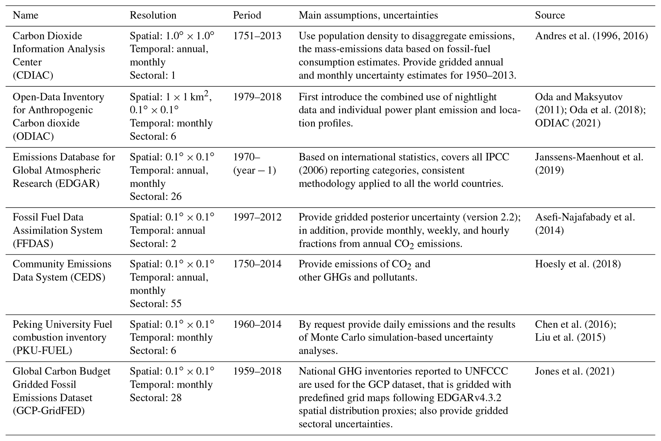
Emission fields are often supplied through emission inventories. Bottom-up emission inventories start from human activity statistics. Emission factors are defined for each activity and provided at the international or country level (e.g. national greenhouse gas inventory report, NIR). Such inventories need to be gridded and characterized with uncertainties to represent a prior dataset useful for numerical modelling. Table 1 shows examples of most commonly used global gridded CO2 emission datasets; for more details see Cong et al. (2018, Table 1), Janssens-Maenhout et al. (2019, Table 3), Andrew (2020), and Jones et al. (2021).
Only four datasets from Table 1 provide uncertainty estimates, namely CDIAC, FFDAS, PKU-FUEL, and GCP-GridFED. CDIAC uncertainties have no sectors and include contributions from the tabular fossil fuel CO2 emissions (assigned per seven country types; values are constant over time), geography map (power plant location), and population map (has details in both time and space and used to distribute fossil fuel CO2 emissions). Population map uncertainty strongly dominates in the generated gridded fossil fuel CO2 uncertainties (Andres et al., 2016). CDIAC uncertainties have no sectoral distribution and are presented on a 1.0∘ × 1.0∘ grid. FFDAS provides only posterior uncertainties, which are based on a model inversion. These posterior uncertainties could be used as prior uncertainties for separate inversion systems. However, this would make the characterization of uncertainty more complex if there were similarities in the model and observations used. PKU-FUEL uncertainty estimates of CO2 emission maps, associated with uncertain fuel data and uncertain activity data in the spatial disaggregation process, are based on Monte Carlo ensemble simulations. Input data were randomly sampled 1000 times from an a priori normal uncertainty distribution with a certain coefficient of variation: for fuel consumptions from ships and aviation the sector coefficient of variation is set to be 20 %, for the wildfires sector 18 %, for all other fuel data 10 %, and for combustion rates 20 % (Marland et al., 2003; Marland et al., 2006; Wang et al., 2013; Oda et al., 2019). GCP-GridFED focusses strongly on the fuel disaggregation for the global CO2 emissions, for which a detailed assessment of the uncertainty has not yet been published.
2.1 Purpose and UNFCCC context
Intercomparisons of global greenhouse gas (GHG) emission inventories were carried out (e.g. Cong et al., 2019; Petrescu et al., 2020) to better understand discrepancies and missing or lesser-known sources. The United Nations Framework Convention on Climate Change (UNFCCC) experts, reviewing national GHG inventories on a yearly basis, are keen to know which sectors or fuels need extra attention for an inventory that complies with the principles of transparency, accuracy, consistency, completeness, and comparability (TACCC principles). Discrepancies are often related to the different interpretations of definitions or to missing information (statistics and/or measurements). When focussing on global emission datasets, which are calculated bottom-up following the Intergovernmental Panel on Climate Change (IPCC) 2006 Guidelines for National Greenhouse Gas Inventories, then the discrepancy using different definitions disappears, while the lack of information becomes strongly apparent for certain regions. More information costs time and effort when compiling a global dataset in a consistent way. Therefore, it is of paramount importance to prioritize the additional information needs and the weaknesses in the inventory with sources of large uncertainty in intensity or variability.
The IPCC has been addressing uncertainty from the beginning. Methodology, data, and data sources in this paper were taken from IPCC (2006) guidelines and their refinements (IPCC, 2019). Also, the assumptions are based on IPCC (2006), so all emissions are considered to be fully uncorrelated with activity (and so with sector and type) (i.e. all activities from IPCC (2006) are fully uncorrelated with each other) for the calculation of the uncertainty as well as of the covariance matrices.
While the UNFCCC sticks to national inventories, the atmospheric modelling community needs spatially distributed data. This adds an extra uncertainty to the emission grid maps, not evaluated with the uncertainty in the proxy data but which needs an assessment of the representativeness of the selected proxies for distributing the emissions. The point sources, leading to large plumes, were prioritized for being treated separately with more data. These consisted of super power plants, which are defined as a large power plant or a group of closely located power plants (operating at maximum capacity and availability), causing CO2 plumes from a single grid cell with a CO2 flux ≥ 7.9 × 10⁻⁶ . According to expert knowledge, the upper-half range of uncertainty for super power plants is not larger than +3.0 %, whereas for small plants whose operation is decided based on day-to-day needs, this can reach up to +15.0 %. In this paper, 30 grid cells of 0.1∘ × 0.1∘ from 12 countries were identified, representing these super power generators (896.7 Mt of the energy sector) and including large plants from China, Russia, and India (for the detailed ranking of the power plant sites as a function of their emission intensity, refer to the Supplement, Sect. S1). The power plant coordinates were checked to avoid the need for an uncertainty related to their positioning. The remaining power plants (not super power generators), over 30 000, could not be checked to the same extent and therefore are recommended in a second emission group.
2.2 Generating uncertainty input for transport models
The uncertainty calculation methodology and initial uncertainty values (i.e. activity data and emission factor uncertainties per CO2-emitting activity) are both taken from IPCC (2006) and its refinements (IPCC, 2019). The following terminology is used to ease the explanation: “activity” – IPCC (2006) activities which result in anthropogenic CO2 emissions in the yearly budget (a long-cycle carbon), “sector” – combination of different activities that are measured or reported together (that have emission budget data), “group” – combination of different sectors that have emission budget data purely for modelling or comparison needs.
In general, uncertainties are calculated in three steps: (i) sector uncertainties (based on emission factors and activity data uncertainties), (ii) annual grouped uncertainties, and (iii) monthly grouped uncertainties. By default, all calculations are performed separately for upper- and lower-half ranges of uncertainties and sector and/or group combined uncertainties, where upper- and lower-half ranges of uncertainty are in percent.
2.2.1 Calculating sector uncertainties
The initial 92 IPCC (2006) activity uncertainties are combined into sectors for which the user has emission budget data1, following Eqs. (1) and (2):
where combined uncertainties UCactivity_i per activity i were calculated using uncertainties for emission factors EFactivity_i and activity data ADactivity_i in percent provided in IPCC (2006) and its refinements (IPCC, 2019);
where combined uncertainties UCsector_j per sector j were calculated with the error propagation method, taking into account particularly for that sector activity combined uncertainties UCactivity_1, UCactivity_2, … , UCactivity_n used in percent.
2.2.2 Group annual uncertainties
This concerns the further grouping of the combined IPCC (2006) sectors according to the user needs into groups and calculation of group yearly uncertainties. Usually, there are computational restrictions for operational modelling: the number of emission input fields read by the model cannot be too large, or emission values are too low to be distinguishable from a global or large regional modelling perspective, so some sectors need to be merged. In addition, instantaneous local emission data as an aggregated total might be rather uncertain and hard to evaluate for different emission types all over the world. IPCC (2006) and its refinement (IPCC, 2019) provide the best possible information on how certain emissions are reported on an annual national level.
Sector uncertainties have to be adjusted to consider a country's statistical system development level and its yearly emission budget and log-normal distribution of non-negative emissions and then further combined into group uncertainties for modelling and comparison purposes in the following way (by default all calculations are performed separately for upper- and lower-half ranges of uncertainties):
where corrected uncertainties (UCsector_j)corr per sector j were calculated to take into account large combined uncertainty (100 % ≤ UCsector_j≤ 230 %) and underestimation by the error propagation method in comparison to a Monte Carlo simulation; correction factor FCsector_j is computed based on Frey (2003), and also log-normal adjustment of the emission distribution is computed based on Frey (2003) as detailed in the Supplement, Sect. S3;
where the combined uncertainties UCgroup_k and total emissions Egroup_k per group k were calculated taking into account specifically for that group sector log-normally transformed uncertainties , , …, in percent.
Group upper- and lower-half range values of uncertainty are descriptive but not straightforward to use in numerical modelling (e.g. emission perturbations in ensemble runs, flux inversions), so mean μln and standard σln deviation of the group log-normal distribution are calculated starting from Eq. (7):
where z is a standard normal variable, and parameters μln and σln represent a natural logarithm of group emissions, not the emissions themselves. The lower and upper bounds of the 95 % probability range, which are the 2.5th and 97.5th percentiles, respectively, are calculated assuming a log-normal distribution based on a corrected estimated half range of uncertainty from the error propagation approach and are lower and upper uncertainty values. Taking this into account and using the Z table for 2.5th and 97.5th percentiles p (, mean μln and standard deviation σln of log-normal distribution can be calculated following Eq. (8):
resulting in Eqs. (9) and (10).
where [UCgroup_k]low and [UCgroup_k]high are in percent.
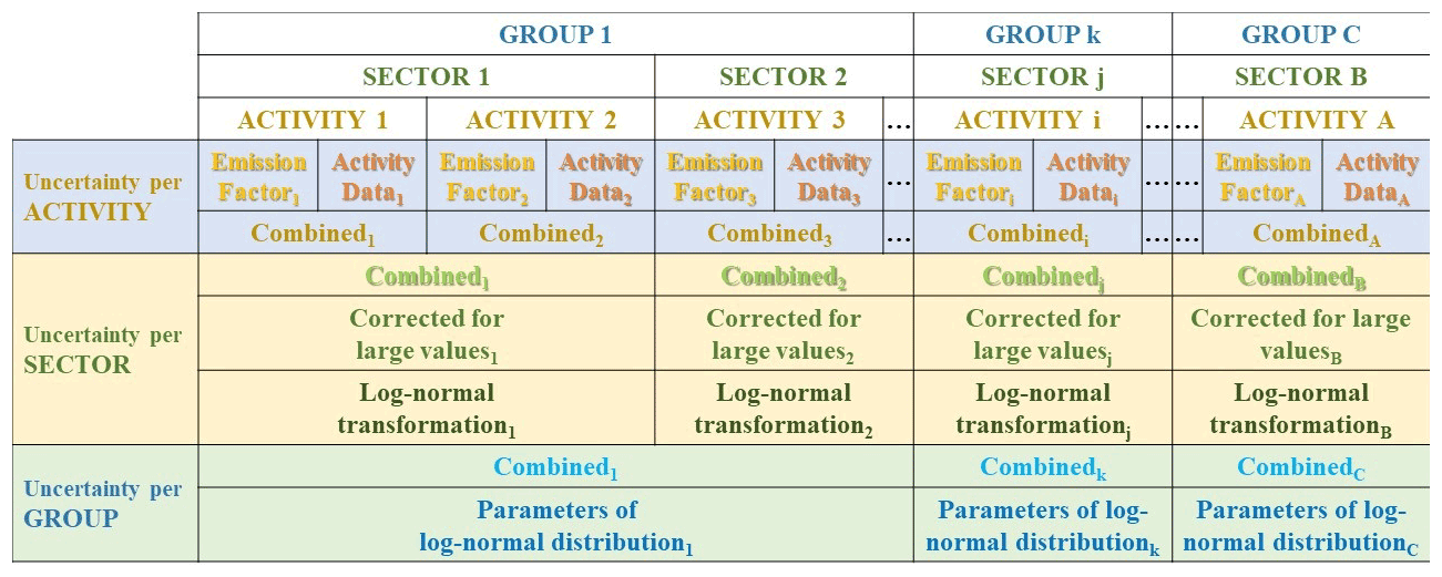
Figure 1 shows a simplified roadmap for yearly uncertainty calculations.
2.2.3 Group monthly uncertainties
The group monthly uncertainties are calculated starting from the yearly uncertainties, which can provide a more appropriate variation than the yearly timescale for operational modelling. In this way, yearly sector uncertainties are adjusted to represent monthly variability (no correlation between months is assumed) and further combined into group monthly uncertainties by means of the following four steps.
-
The same steps as for annual uncertainty calculation are used but based on monthly emission budgets (i.e. uncertainties for IPCC activities are combined to sectors with the error propagation method, corrected for systematic underestimation by the error propagation method, and adapted to have log-normal distribution).
-
The correlation α (an uncertainty-boosting parameter) between yearly and monthly uncertainties is based on an analysis of the variations over the different months following Eq. (11). It is computed to enhance obtained monthly uncertainties as they are the same or even smaller than the yearly ones because empirical equations applied use emission budgets, which are smaller for individual months compared to the yearly values:
where E and UC correspond to sector emission budget and uncertainty in kilotonnes and percent, respectively; YEAR, MONTH1, MONTH2, … , MONTH12 are yearly and monthly (January, February, … , December) values. Equation (11) is based on the rule for combining uncorrelated uncertainties under the addition of the error propagation equation (see Eq. 5) and the assumption that each month's uncertainty should be enhanced (boosted) by the same value.
-
The prior yearly sector uncertainties are multiplied by the boosting parameter (specific per country and emission sector), and the results are used as a first guess of prior month sector uncertainties.
-
The calculation steps (1) to (3) are iterated to find the best boosting parameter as the best fit between yearly and combined 12-month uncertainties, with the incremental step below a given acceptable threshold from Eq. (11) for each country and emission sector. With this optimum boosting parameter, monthly uncertainties per sector are calculated and then merged into groups, with a log-normal distribution of CO2 emissions.
Detailed information on each Unix shell script included in the anthropogenic CO2 emission uncertainty calculation tool CHE_UNC_APP (Choulga et al., 2021) is provided in the Supplement, Sect. S4.
2.2.4 Remarks about the fuel dependence and assumptions concerning correlation
It should be noted that IPCC (2006) provides default emission factor values for different fuels in transport-related activities (e.g. railways, aviation). Detailed fuel consumption information per IPCC activity that results in a long-cycle carbon was not available, and instead the most typical and consumed (common) fuel type (or its emission factor value) was used:
-
aviation cruise (1.A.3.a_CRS), climbing and descent (1.A.3.a_CDS), and landing and take-off (1.A.3.a_LTO) – jet kerosene;
-
road transportation (1.A.3.b) and pipelines, off-road transport (1.A.3.e) – most typical emission factor uncertainty;
-
shipping (1.A.3.d) – composition of 80 % diesel and 20 % residual fuel oil;
-
railways (1.A.3.c) – diesel.
It should also be noted that some uncertainty ranges for emission factors and/or activity data in IPCC (2006) and its refinements (IPCC, 2019) are not symmetrical and have higher uncertainty values for the lower-half range than for the half-range (or vice versa) due to input from expert knowledge or available in situ data, which then leads to the same pattern in final prior uncertainty range.
It should finally be noted that according to the IPCC (2006), all anthropogenic CO2 emissions are assumed to be fully uncorrelated; hence the prior error correlations between grid cell emissions from the same sector or group should be assumed negligible if country- and/or sector-specific information is lacking.
The method explained above has been applied to the EDGARv4.3.2_FT2015 dataset to prepare prior uncertainty information for the ECMWF Integrated Forecasting System (IFS) model.
3.1 Data input
In this example, 2015, the year of the Paris Agreement and reference for several Nationally Determined Contributions, is chosen as a base year to analyse anthropogenic CO2 budgets (i.e. global, regional, national) from different sources (i.e. global statistics, national reports), benefitting the availability of observations (both in situ ground and spaceborne) as well as reported and verified emission inventories.
Table 2Grouping of anthropogenic long-cycle carbon CO2 emission sectors into groups. Note provides main information and typical fuel type; global emission budgets for 2015 in megatonnes provides values for EDGARv4.3.2_FT2015 (total sum 35 986.5 Mt) and CHE_EDGAR-ECMWF_2015 (total sum 35 995.2). Italics represent values with the biggest differences; asterisks (∗) represent values that were replaced from EDGARv4.3.2
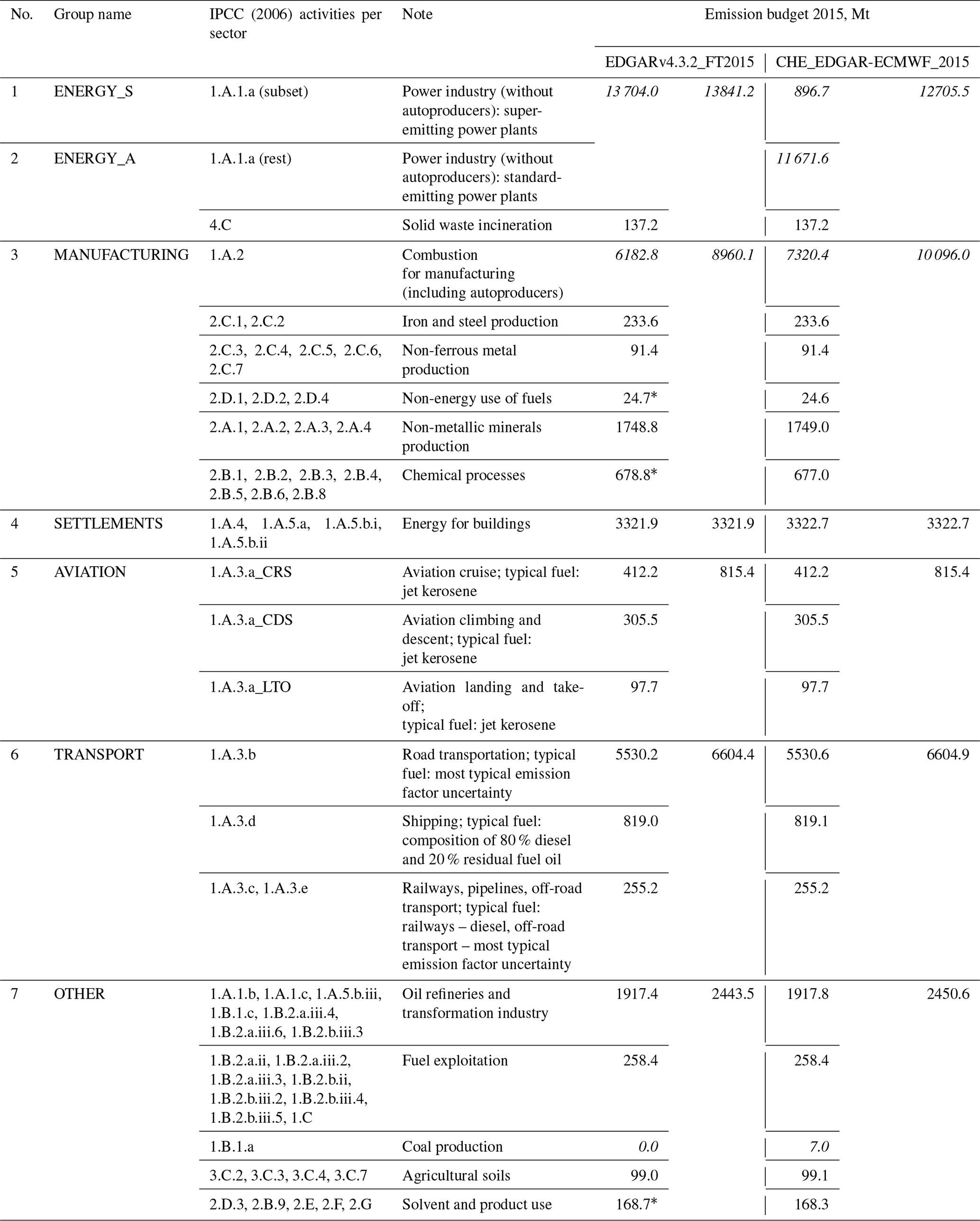
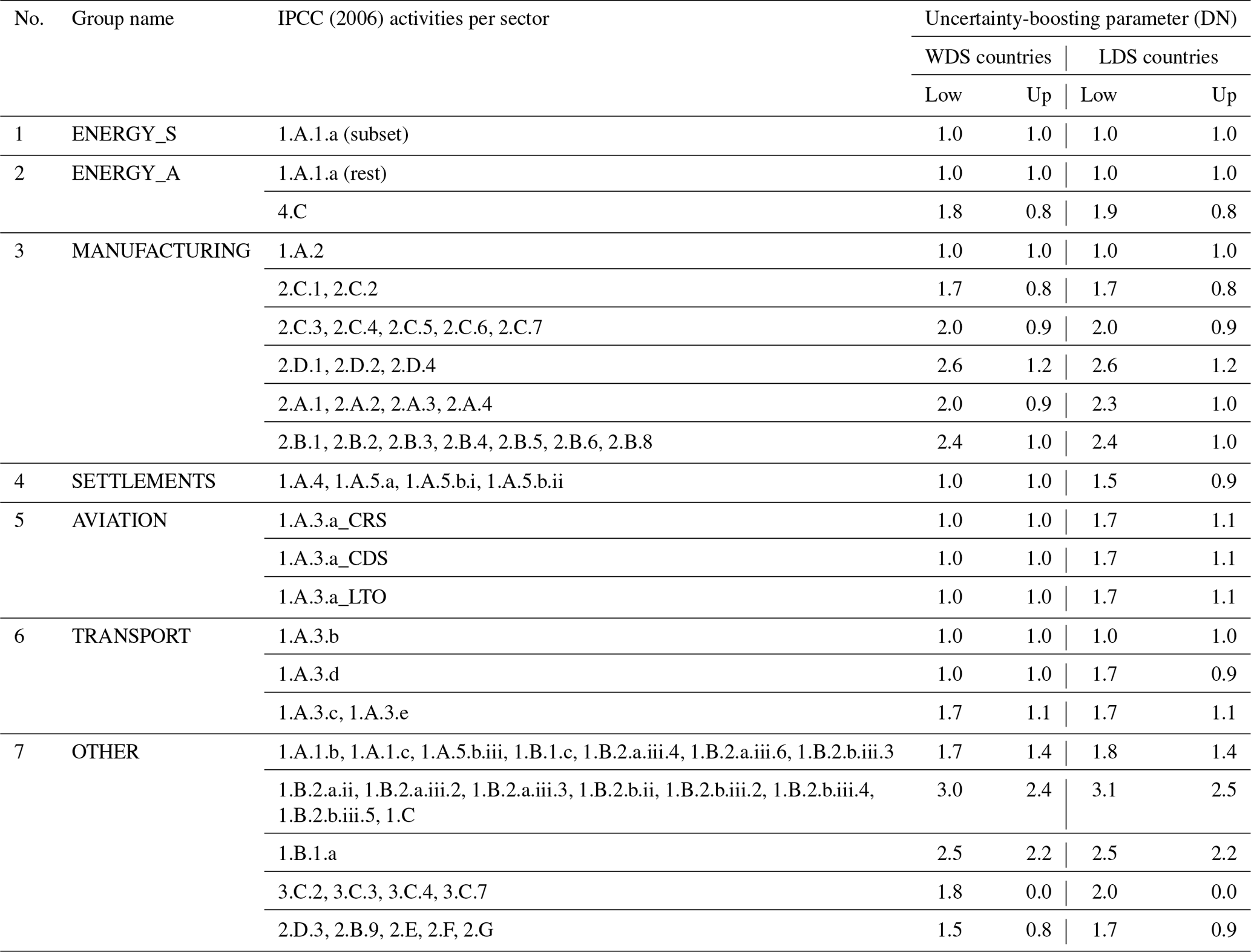
Following IPCC (2006) and its refinements (IPCC, 2019), starting from the global fossil CO2 grid maps of EDGAR inventory versions 4.3.2 (Janssens-Maenhout et al., 2019) and 4.3.2_FT2015 (Olivier et al., 2016a), for 2012 and 2015, respectively, an updated emission dataset CHE_EDGAR-ECMWF_20152 (Choulga et al., 2020) is derived. The EDGARv4.3.2 dataset is improved by correcting the allocation of the autoproducers to the manufacturing sector instead of the energy sector. Autoproducers are defined by the International Energy Agency (IEA) and include the energy (electricity and heat) generated by an industry for its own use, mostly for the manufacturing. An extra emission source of fugitive CO2 from coal mines is also added, following the recommendations from IPCC (2019). Even though this emission source is not that large globally, usually the coal seam gas is composed dominantly of methane (CH4), but in some coal mines (in Australia and also in Brazil) seam gas consists predominantly (> 95 %) of CO2 (Beamish and Vance, 1992), leading to significant atmospheric CO2 concentration increases. An additional map for CHE_EDGAR-ECMWF_2015 with coal mining emissions from underground mines has been generated following the IPCC (2019) default values and the coal mining activity of CH4 emission grid maps from hard and brown coal production in EDGARv4.3.2 (for more information refer to the Supplement, Sect. S2). For the update from 2012 to 2015 the fast-track approach of Olivier et al. (2016b) is used. The initial 92 IPCC activity uncertainties are combined into 20 EDGAR sectors for two distinct country types with well- and less well-developed statistical infrastructures (i.e. country's ability to register different emissions, meaning tabulate even very small emissions or only major ones, respectively). For the input to the IFS model the emission sectors are grouped in seven groups, with one group devoted to super power plants. Table 2 shows activity and sector grouping and emission budget differences between EDGARv4.3.2_FT2015 and CHE_EDGAR-ECMWF_2015 datasets due to reallocation of the autoproducers from the energy sector (−8 %) to the manufacturing sector (+18 %) and due to the extra emission source of diffusive coal mine CO2.
3.2 Model constraints
The operational IFS model is used to provide global CO2 forecasts using the gridded prior emissions previously described (Agusti-Panareda et al., 2014; Agusti-Panareda et al., 2019). A prototype 4D-Var inverse modelling system is currently under development to monitor anthropogenic CO2 emission using the IFS. There is also an ongoing development to extend the window length beyond 24 h using an ensemble-based methodology.
The uncertainties derived for the seven groups described here have been used to generate an ensemble of forecasts for 2015 based on the operational IFS ensemble system (McNorton et al., 2020). This provides a representation of the model uncertainty and an estimation of the expected signal-to-noise ratio for a future inverse modelling system. Random seeds for each group and country were applied to the normalized log-normal mean μln and standard deviation σln to generate emission scaling factors, which were then used for 50 ensemble members.
Primarily, the derived emission uncertainties presented here are envisaged for use as prior errors within atmospheric inversion frameworks. Aggregation of emission sectors into seven groups is required for computational efficiency and to reduce the dimensions of the inverse problem. To resolve collocated emissions, further information is required about spatial correlations and/or co-emitted species (e.g. nitrogen oxides, NOx). Within the IFS inversion prototype, the log-normal normalized standard deviation outlined in the previous section is used to provide the uncertainty values to prevent negative scaling factors.
3.3 CHE_EDGAR-ECMWF_2015 output
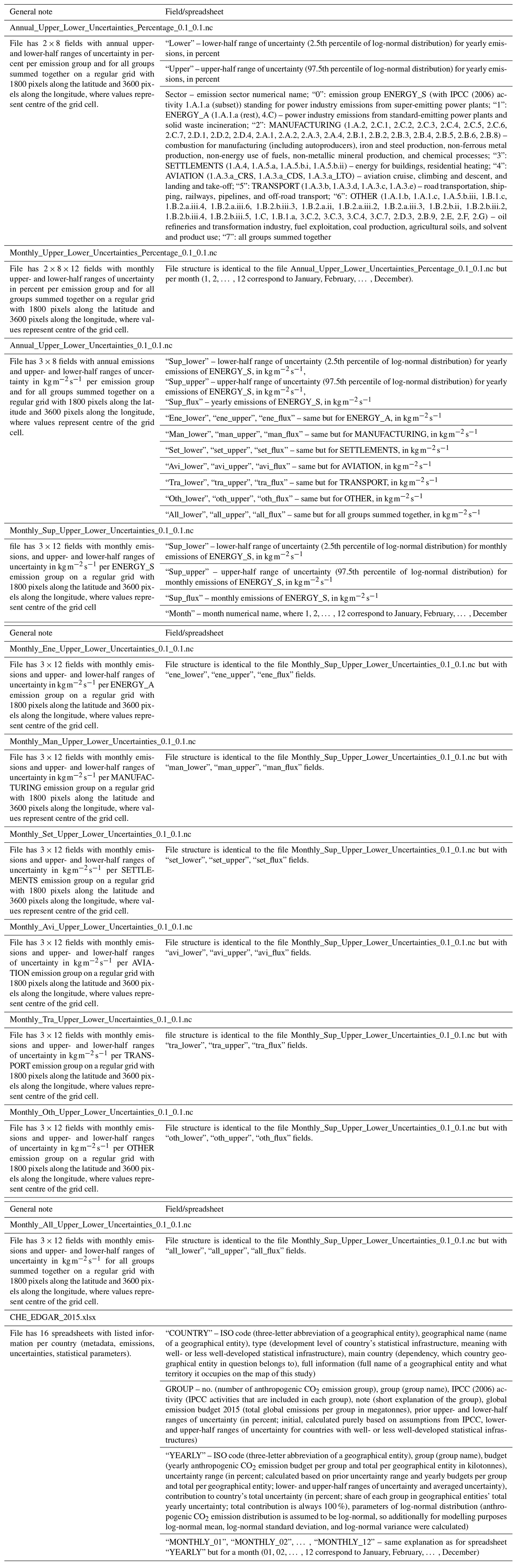
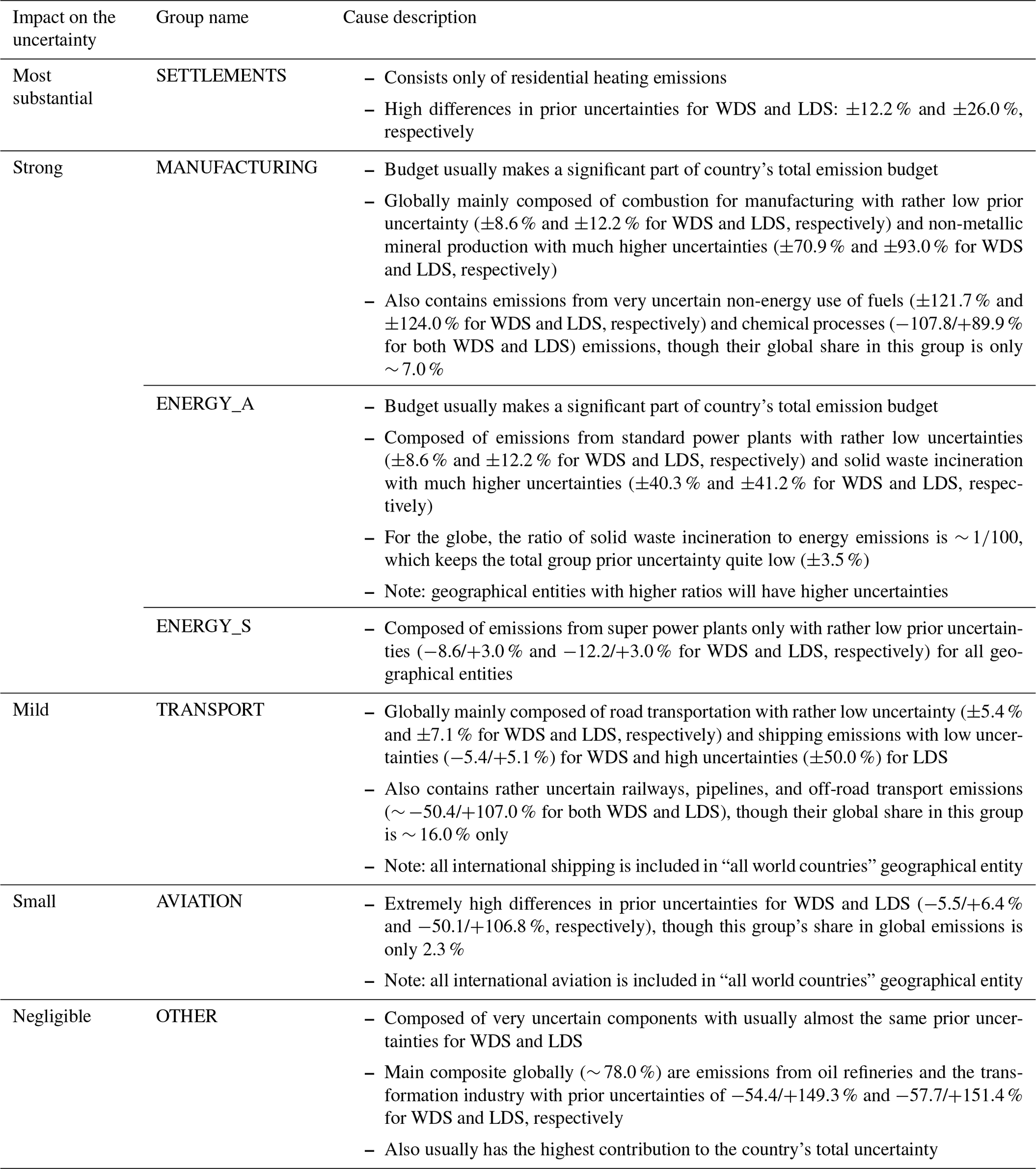
The new CHE_EDGAR-ECMWF_2015 dataset with anthropogenic fossil CO2 emissions and their uncertainties was compiled and tested at ECMWF. The fossil CO2 emissions include all long-cycle carbon emissions from human activities, such as fossil fuel combustion, industrial processes (e.g. cement), and product use, but excludes emissions from land-use change and forestry. Human CO2 emission inventories were processed into gridded 0.1∘ × 0.1∘ resolution maps to provide an estimate of prior CO2 emissions, aggregated in seven main emissions groups: (1) energy production by super-emitters, (2) energy production by standard emitters, (3) manufacturing, (4) settlements, (5) aviation, (6) other transport at ground level, and (7) others, with an estimation of their uncertainty and covariance. Aggregation of the IPCC activities and sectors into groups was based on similarities between the magnitude of uncertainty, the spatiotemporal correlation, and co-emission factors of each sector. It is assumed that each emission group is fully correlated with itself and fully uncorrelated with any other group (only diagonal values of the 7 × 7 group covariance matrix for the atmospheric transport model are non-zero and equal to log-normal variance). The CHE_EDGAR-ECMWF_2015 data are freely available (https://doi.org/10.5281/zenodo.3967439; Choulga et al., 2020) and consist of 11 grid maps in NetCDF format and one Excel file with information on anthropogenic CO2 emissions and their uncertainties. For detailed information on each file see Table 3.
3.4 Example of uncertainty calculation
Table 4 shows a step-by-step example of how yearly uncertainties are calculated, and Fig. 2 shows plotted probability density functions based on computed log-normal parameters. The example shows calculations for the TRANSPORT group that consists of several emission sectors. The example shows two countries with different statistical infrastructure development levels (the country with well-developed statistical infrastructure is Germany, and the country with less well-developed statistical infrastructure is the Russian Federation) and significant differences in emission budgets.
Table 4Yearly uncertainty calculation steps. Example shows TRANSPORT group uncertainty calculations for Germany (DEU) and the Russian Federation (RUS), countries with a well- (WDS) and less well-developed statistical infrastructure (LDS), respectively. (a) Preparatory step (data collection) – same values are applied for all countries with the same development level of statistical infrastructure. (b) First step – same values are applied for all countries with the same development level of statistical infrastructure. (c) Second step – values are specific per geographical entity considering countries' development level of statistical infrastructure and emission budget (values are from CHE_EDGAR-ECMWF_2015); SD stands for standard deviation.
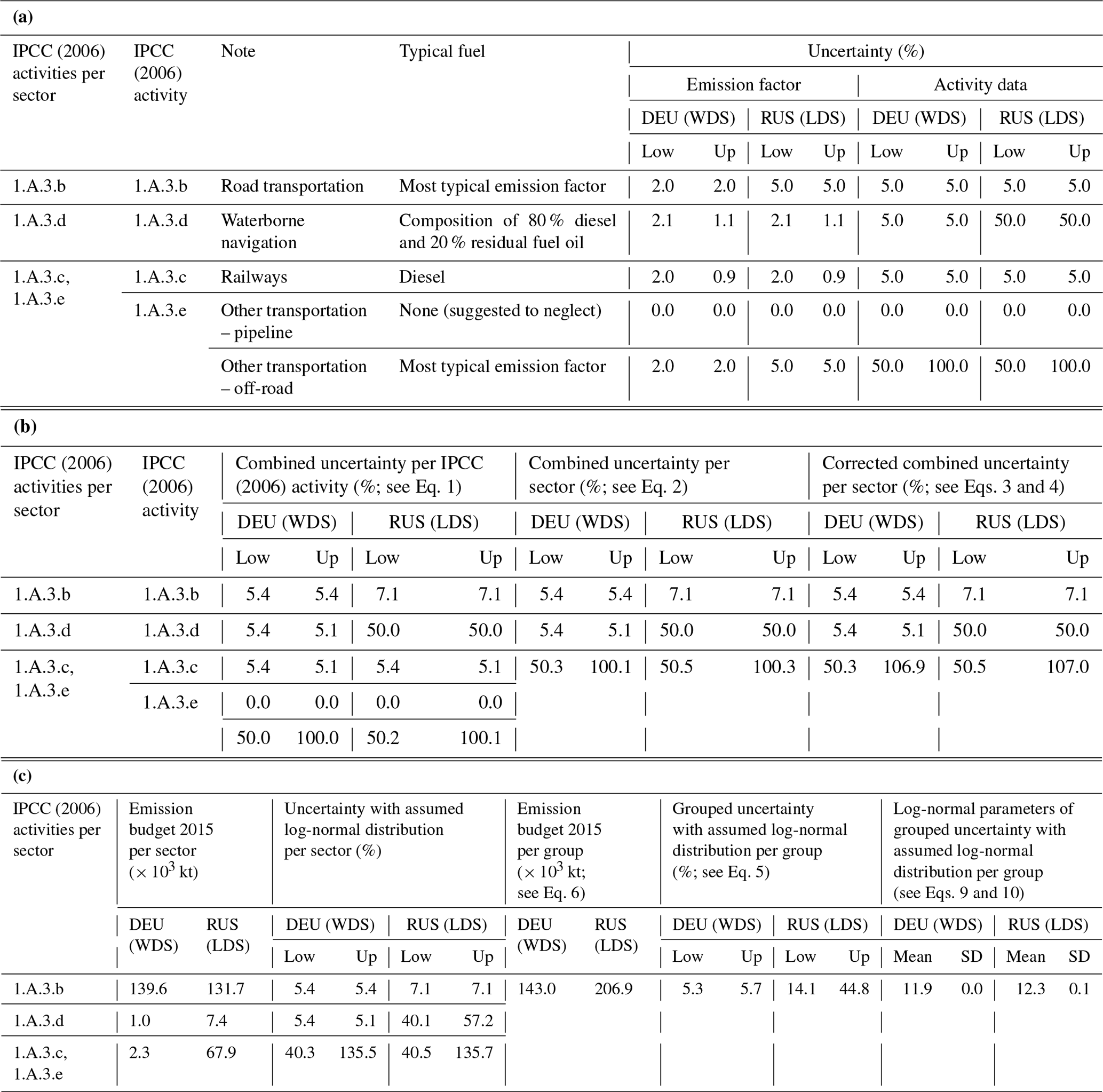
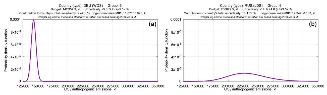
Figure 2Probability density functions (for Germany a and the Russian Federation b) based on computed log-normal mean and standard deviation for the TRANSPORT group.
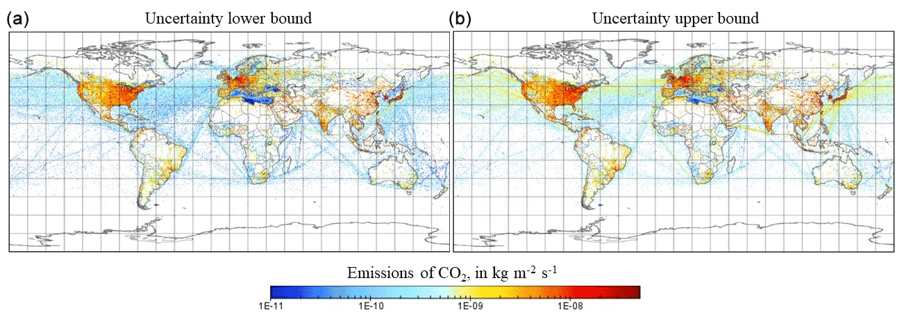
Figure 3CO2 emission flux uncertainties (a lower- and b upper-half ranges of uncertainty) for the TRANSPORT group in .
Calculated yearly and monthly uncertainties per country and emission group were assigned to each grid box on the global map. National uncertainties were applied uniformly across each country. Figure 3 shows an example of the upper and lower uncertainty limits of anthropogenic CO2 emission flux for the TRANSPORT group. It should be noted that uncertainties related to the spatial distribution (representativeness of the proxy data and their uncertainty) should be much higher than the ones presented in this study. This research does not address uncertainties related to the spatial distribution. In the future it is planned to address these uncertainties too, for example by following Oda et al. (2019) to characterize spatial patterns of the disaggregation errors in the emission maps.
4.1 Comparison of total uncertainty in global CO2 emission datasets
Calculated emissions and uncertainties in fossil CO2 have been compared to other global datasets based on the country-specific data reported to UNFCCC and on fuel-specific data reported in the energy statistics of IEA. The global values and their uncertainty at a 2σ range for the CHE_EDGAR-ECMWF_2015 dataset show a lowest value of −4.7 %/+9.6 %, or ±7.1 %; see Table 5. This result might be attributed to the methodology, in particular considering that (i) all calculations were done at the country level and then aggregated to the global level assuming no correlation following IPCC (2006); (ii) all calculations were done separately for upper- and lower-half ranges of uncertainty to preserve original information with asymmetric confidence intervals for large uncertainties (not required for the Approach 1 described in IPCC (2006), in which only the higher uncertainty value of the asymmetric interval should be used, leading to artificial inflation of uncertainty upper or lower limit); and (iii) in this study proxy grid map uncertainties are not considered.
Table 5Comparison of global anthropogenic CO2 emission uncertainty at 2σ associated with certain emission datasets.

∗ The difference between ODIAC and CDIAC gridded data is 3.3 %–5.7 % (Oda et al., 2018).

Figure 4Main emission group that contributes to the total uncertainty per grid cell – global region.
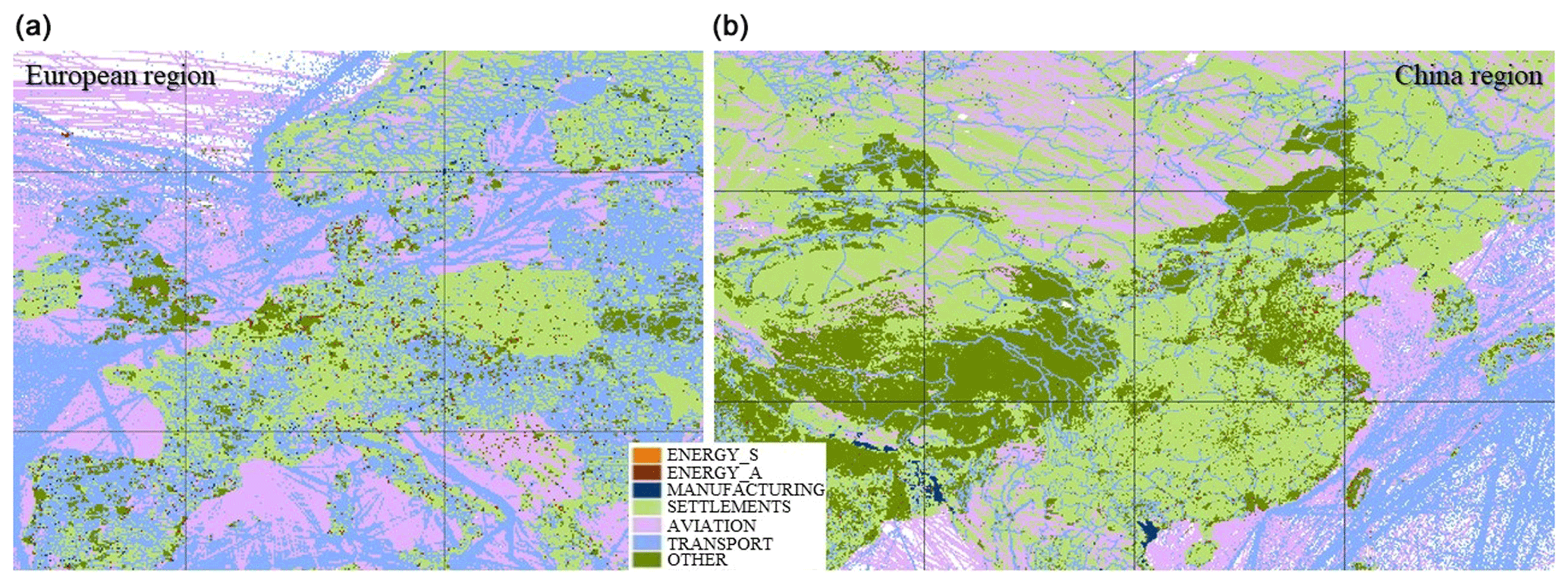
Figure 5Main emission group that contributes to the total uncertainty per grid cell – European (a) and China (b) regions.
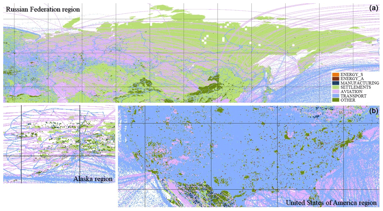
Figure 6Main emission group that contributes to the total uncertainty per grid cell – the Russian Federation (a) and the United States of America (b) regions.
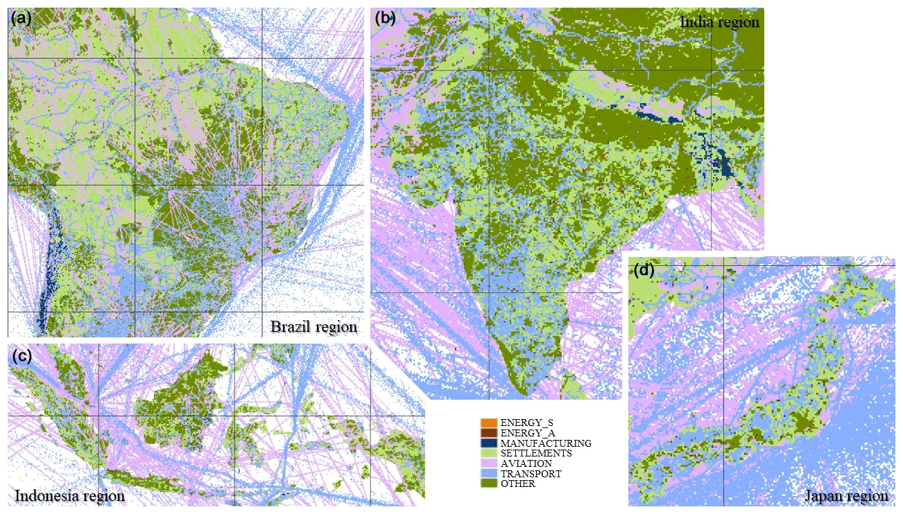
Figure 7Main emission group that contributes to the total uncertainty per grid cell – Brazil (a), India (b), Indonesia (c), and Japan (d) regions
The contribution of each emission group to the total uncertainty per grid cell is assessed. Figures 4–7 show which group contributes the most to the total uncertainty per grid cell. The TRANSPORT group contributes most to the grid cell uncertainty over the Unites States of America (due to road and off-road transport) and over the ocean (due to shipping). The AVIATION group contributes most over main flight routes all over the globe. The OTHER group contributes the most over agricultural areas and regions with oil refineries and transformation industry and fuel exploitation. The MANUFACTURING group contributes most over industrial areas (e.g. in Vietnam and Bangladesh). The ENERGY_A (and ENERGY_S) group contributes the most over power plant (and super power plant) location grid cells (e.g. South Africa). The SETTLEMENTS group contributes the most to the grid cell uncertainty over either very densely or very sparsely populated areas.
4.2 Dependence of the country-specific statistical infrastructure
Also, some specific geographical areas are analysed: chosen to be among the most emitting in total or per emission group and the most typical or most influential for a certain region. A list of these geographical entities and development levels of their statistical infrastructures is presented in Table 6.
Table 6List of selected geographical entities with their statistical infrastructure's development levels.
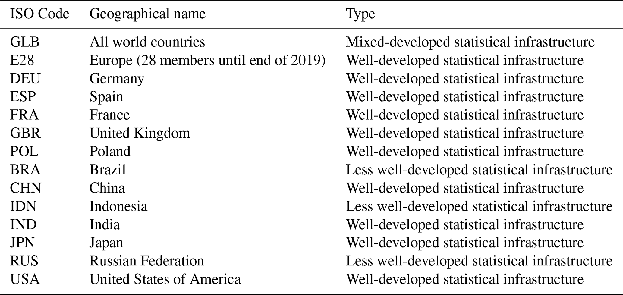
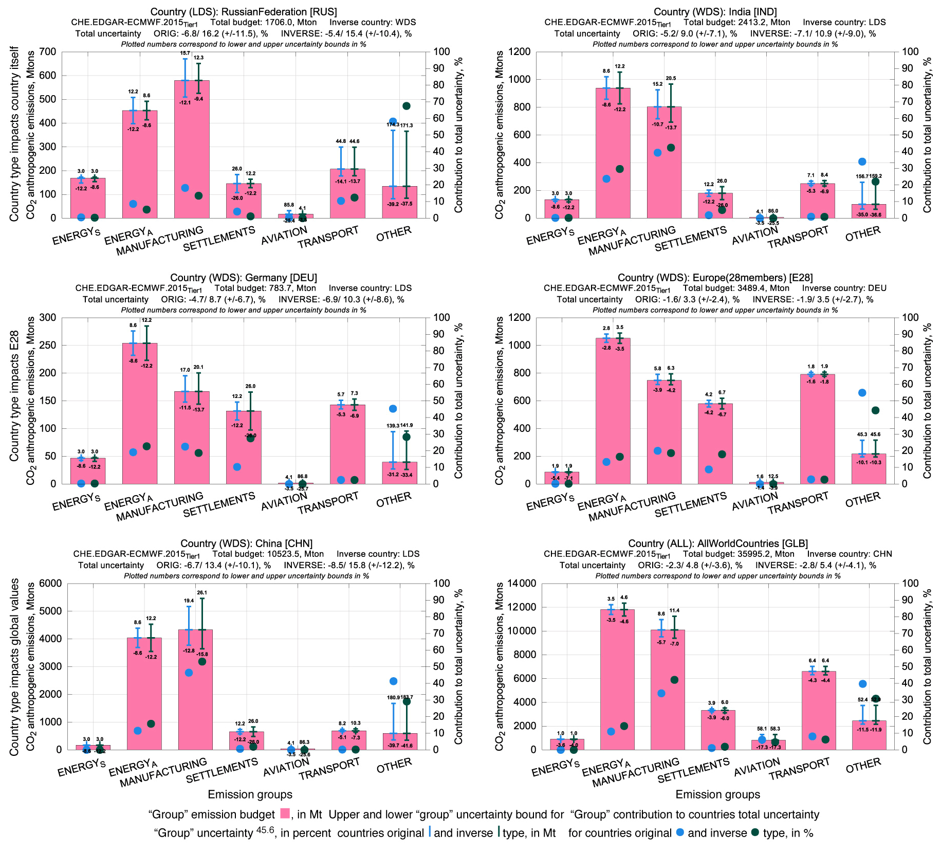
Figure 8Emission budgets, uncertainties, and contributions in percentage to the total uncertainty in the country with their original and switched (inverse) types (countries with well- and less well-developed statistical infrastructures – WDSs and LDSs, respectively): impacting mainly the country itself, e.g. the Russian Federation (RUS) and India (IND); impacting also Europe (E28), e.g. Germany (DEU); impacting even global values, e.g. China (CHN).
Table 7Influence of country's statistical infrastructure (countries with well- and less well-developed statistical infrastructures – WDSs and LDSs, respectively) on emission uncertainty.
In order to see how the development level of country's or geographical entity's statistical infrastructure influences the emission uncertainty in that country or geographical entity itself and (possibly) the globe, uncertainty calculations for selected entities were performed twice – with their original and switched types (i.e. a country with a well-developed statistical infrastructure becomes a country with a less well-developed statistical infrastructure and vice versa). More details on a geographical entity's statistical infrastructure development level (e.g. how it was determined) are given in the Supplement, Sect. S5. Figure 8 shows sectoral emission budgets, uncertainties, and contributions in percentage to the total uncertainty in a country or geographical entity with its original and switched statistical infrastructure development levels. The biggest impact of development level change occurs for countries with larger emission budgets. On average, total uncertainties in selected countries (see Table 6) changed by 1 %–2 %; group uncertainties changed in line with prior uncertainties and countries' emission budgets, as reported in Table 7.
Alterations in some countries' (e.g. Germany, France) statistical infrastructure's development levels lead to changes in uncertainties in Europe (28 members until end of 2019), with the most substantial change for the SETTLEMENTS group (e.g. 2.5 % and 1.0 %, respectively). Huge changes (> 10.0 %) in Europe's (28 members until end of 2019) AVIATION group's uncertainty percentage value can be due to the variation in statistical infrastructure development level for Germany, United Kingdom, France, or Spain, though this group's contribution to Europe's total uncertainty remains negligible. Alterations in statistical infrastructure development levels for China or the United States of America modify even global uncertainties because these countries substantially contribute to the total global emission budget; e.g. China emits ∼ of the global anthropogenic CO2 budget and can change global total uncertainty up to 0.5 %.
4.3 Effect of increasing temporal resolution from yearly to monthly
To increase the emission temporal resolution, monthly emissions and their uncertainties were calculated combining yearly emissions, monthly
multiplication factors, and adapted uncertainty calculation methodology (see Sect. 2.2). Prior yearly uncertainties were multiplied by a dimensionless
uncertainty-boosting parameter α (same value for each month) to compute prior monthly uncertainties, which were further used together with
monthly emission budgets for countries' monthly uncertainty calculation. Monthly uncertainties (just like yearly uncertainties) are determined by
empirical formulas from IPCC (2006) with monthly emission budgets (weighted with the total number of days in a month). The dimensionless uncertainty-boosting parameter α is applied; see Table 8 for most common values for countries with well- and less well-developed statistical
infrastructures per sector. Boosting parameters become active (α≠1) when absolute uncertainty values are ≥ 25.0 %, and
α increases with the increase in absolute uncertainty following a third-order polynomial. For lower-half ranges of uncertainty, α has larger
values and steeper growth than for upper-half ranges of uncertainty
(e.g. −25.0 % ![]() α = 1.5 and
−124.0 %
α = 1.5 and
−124.0 % ![]() α = 2.6,
+25.0 %
α = 2.6,
+25.0 % ![]() α = 0.8 and
+124.0 %
α = 0.8 and
+124.0 % ![]() α = 1.2;
α = 1.2; ![]() means
“corresponds to”), and α behaves in the same way for countries with well- and less well-developed statistical infrastructures. Discrepancies
in a different geographical entity's (country's) boosting parameters might be for several reasons. The main ones are (i) sector emissions were zero
(e.g. super power plant emissions of the energy sector had no emissions), and (ii) sector uncertainties were ≥ 50.0 % and needed to be
adapted accordingly to log-normal distribution (this is the case for the agricultural soils sector with prior uncertainties
−70.7/+0.0 % for countries with well- and less well-developed statistical infrastructures; discrepancies from
Table 8 for agricultural soils are France – α = 1.8/3.1, UK – 1.8/7.2, China – 1.8/8.4, Japan – 1.8/10.8, Brazil – 1.8/0.0, and the Russian
Federation – 1.8/5.6, where the first value is for the lower-half range of uncertainty, and the second value is for the upper-half range of uncertainty).
means
“corresponds to”), and α behaves in the same way for countries with well- and less well-developed statistical infrastructures. Discrepancies
in a different geographical entity's (country's) boosting parameters might be for several reasons. The main ones are (i) sector emissions were zero
(e.g. super power plant emissions of the energy sector had no emissions), and (ii) sector uncertainties were ≥ 50.0 % and needed to be
adapted accordingly to log-normal distribution (this is the case for the agricultural soils sector with prior uncertainties
−70.7/+0.0 % for countries with well- and less well-developed statistical infrastructures; discrepancies from
Table 8 for agricultural soils are France – α = 1.8/3.1, UK – 1.8/7.2, China – 1.8/8.4, Japan – 1.8/10.8, Brazil – 1.8/0.0, and the Russian
Federation – 1.8/5.6, where the first value is for the lower-half range of uncertainty, and the second value is for the upper-half range of uncertainty).
Table 8Dimensionless (DN) lower- and upper-half-range boosting parameter for countries with well- and less well-developed statistical infrastructures – WDSs and LDSs, respectively.
In general, Brazil, Indonesia, and India have a very weak yearly cycle with quite high monthly uncertainties throughout the year. The globe, Europe (28 members until end of 2019), Germany, Spain, France, United Kingdom, Poland, China, Japan, the Russian Federation, and the United States of America have more pronounced yearly cycles, most significant for the SETTLEMENTS and ENERGY_A (and ENERGY_S where present) groups and less significant for the AVIATION, TRANSPORT, and MANUFACTURING groups. This is in line with the monthly profiles applied in EDGARv4.3.2 for northern and southern temperate zones and the Equator; see Janssens-Maenhout et al. (2019). In the summer months for the northern temperate zone, a strong decrease in SETTLEMENTS and ENERGY_A (and ENERGY_S where present) group emissions was observed, with a light decrease in MANUFACTURING group emissions and a light increase in AVIATION and TRANSPORT group emissions. This corresponds rather well to the assumption that most of the population in the Northern Hemisphere heat their houses during winter and take holidays and travel more during summer.
4.4 Comparison for selected European countries with UNFCCC and TNO data
The CHE_EDGAR-ECMWF_2015 dataset containing seven global gridded fossil CO2 emission flux maps and country- and group-specific emission budgets and uncertainties have been assessed with independent data. Global emission budget values from different datasets are almost never the same; therefore it is important to first identify why estimates differ between datasets. Datasets might use the same country-level information as primary input, though differences in inclusion, interpretation, and treatment of that data lead to diverse results in emissions. It is necessary to try to harmonize data inclusion or omission across datasets to have more clarity in the discrepancies.
For Europe (28 members until end of 2019), Germany, Spain, France, United Kingdom, Poland, Japan, the Russian Federation, and the United States of America, emission and uncertainty data were collected from UNFCCC NIR. The aggregation of the IPCC (2006) activity-specific emissions and uncertainties into seven groups was done assuming no correlation, following IPCC (2006). Although IPCC (2006) has a standard table to report GHG emissions, uncertainties can be reported in less detail by a more general category (e.g. 2.D only instead of 2.D.1, 2.D.2, 2.D.3, 2.D.4), meaning information “harmonization” required lots of careful time-consuming country-specific technical work by the authors of this paper.
The Netherlands Organisation for Applied Scientific Research (TNO) has prepared the first version of their GHG and co-emitted species emission database (TNO_GHGco_v1.1) that covers the entire European domain (at 0.1∘ × 0.05∘ resolution), including CO2 (distinguishing between fossil fuel and biofuel). Initial emission data are from the UNFCCC (common reporting format, CRF, tables) and the European Monitoring and Evaluation Programme (EMEP) of the Centre on Emission Inventories and Projections (CEIP) for air pollutants. These data were harmonized; checked for gaps, errors, and inconsistencies; and (where needed) replaced or completed using emission data from the Greenhouse Gas and Air Pollution Interactions and Synergies (GAINS) model (Amann et al., 2011). Moreover, inland shipping emissions were replaced with the TNO's own estimates, and sea shipping is based on automatic identification system (AIS)-based tracks. Expert judgement is used to assess the quality of each data source and to make choices on which source to use. The resulting emissions were checked in detail regarding their absolute value and trends (Kuenen et al., 2014). In this study emission budgets from 30 TNO sectors (Ingrid Super, Jeroen Kuenen, Antoon Visschedijk, and Hugo Denier van der Gon, personal communication, February 2020), and prior uncertainties calculated from IPCC (2006) and its refinements (IPCC, 2019) are used. In addition, the TNO has provided Tier 2 (Monte Carlo approach) uncertainties based on the same budgets and uncertainties from submitted NIR reports based on a Tier 1 approach. The Monte Carlo simulations were done at the highest detail level (nomenclature for reporting (NFR) sector and fuel type) assuming correlations between certain sectors (for more information see Super et al., 2020), and then emissions were aggregated to groups assuming no correlation.
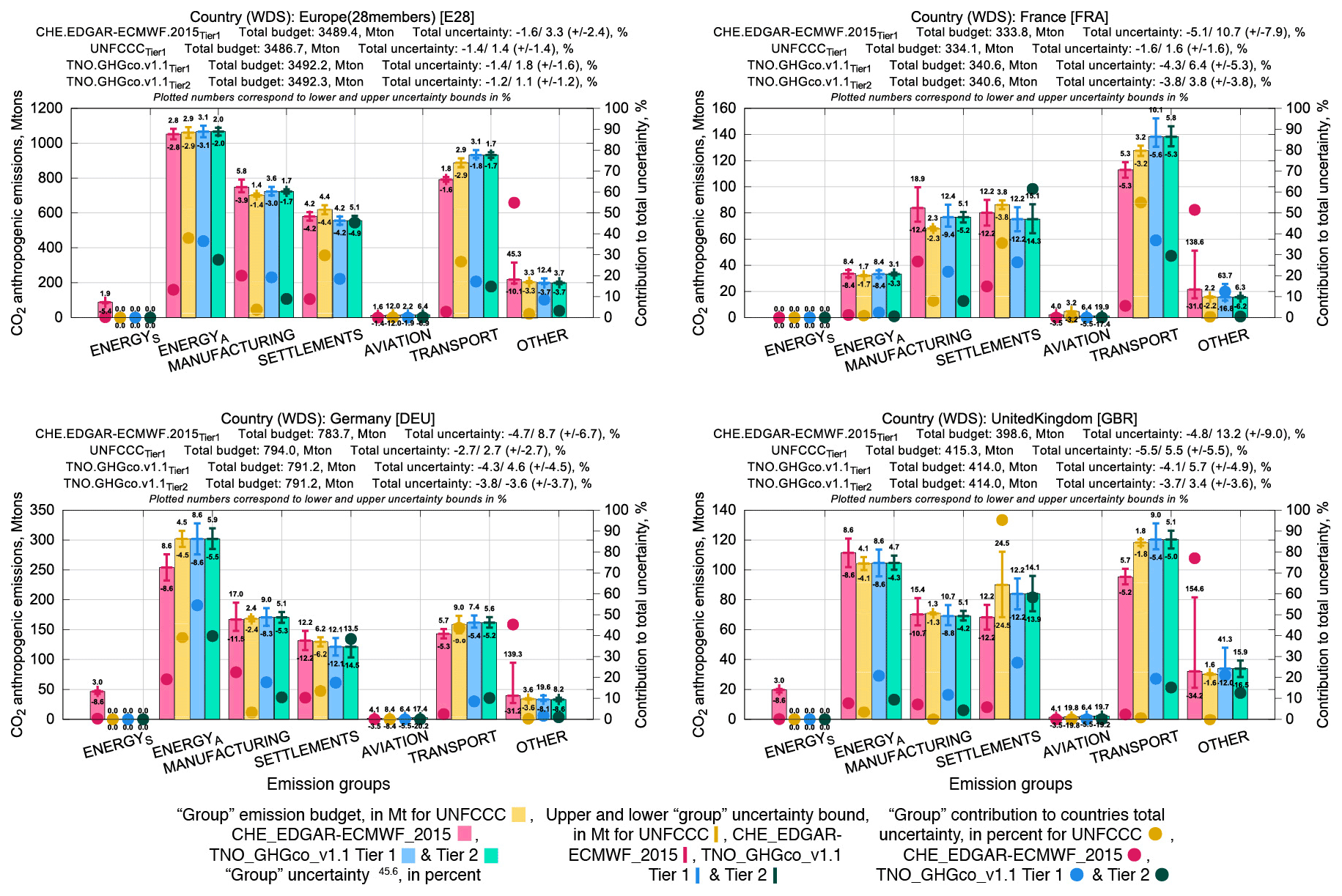
Figure 9Emission budgets, uncertainties, and contributions in percentage to the total uncertainty for Europe (E28), Germany (DEU), France (FRA), and United Kingdom (GBR).
Figure 9 shows emission budgets and uncertainties in megatonnes and contributions in percent to the total geographical entity's uncertainty for Europe (28 members until end of 2019), Germany, France, and United Kingdom with their original statistical infrastructure development types based on data from CHE_EDGAR-ECMWF_2015 (in pink), UNFCCC (in yellow), and TNO_GHGco_v1.1 Tier 1 (in blue) and Tier 2 (in green); plots for Spain and Poland are not shown here. Out of the four different sources, usually UNFCCC and TNO_GHGco_v1.1 Tier 2 uncertainties are the lowest ones and CHE_EDGAR-ECMWF_2015 the highest one. It should be noted that (i) UNFCCC uncertainties were aggregated to groups individually per country as uncertainties are reported in a rather free form and thus could be aggregated from different levels of precision; (ii) uncertainties for Europe (28 members until end of 2019) from CHE_EDGAR-ECMWF_2015 are rather low as they were calculated by aggregating information from 28 countries; and (iii) differences in uncertainties in CHE_EDGAR-ECMWF_2015 with other sources, especially in fuel-dependent emission groups, might be due to biofuels or other fuels (e.g. wood and/or coal for residential heating). Differences in uncertainties between CHE_EDGAR-ECMWF_2015 and TNO_GHGco_v1.1 Tier 1 show additional value in more detailed emission budget knowledge (i.e. where absence of the uncertain glass production activity in the non-metallic mineral production sector decreases overall uncertainty). Differences in uncertainties between TNO_GHGco_v1.1 Tier 1 and TNO_GHGco_v1.1 Tier 2 show additional value in an advanced calculation technique using a more sophisticated, data-demanding Monte Carlo approach instead of simple error propagation. Overall, there is quite good agreement in emission budgets and uncertainties from different sources of emission data.
Emission budgets, Tier 1 uncertainties, and contributions in percentage to the total geographical entity's uncertainty for Japan, the Russian Federation, and the United States of America from CHE_EDGAR-ECMWF_2015 could be compared only with UNFCCC data (plots not shown here). UNFCCC uncertainties are usually lower than the ones calculated in this study. The main reason for that is the use of country-specific emission data and activity data uncertainties, which are lower than default values suggested by IPCC (2006) and its refinements (IPCC, 2019). Only for the fuel-dependent groups (e.g. AVIATION) might UNFCCC uncertainties be higher than in this study as rather uncertain biofuels might be taken into account (note: CHE_EDGAR-ECMWF_2015 does not take biofuels into account). Also, emission budgets reported to the UNFCCC show some differences from the ones from CHE_EDGAR-ECMWF_2015. For Japan, group budgets agree rather well, and the total budget difference is ∼ 1.0 %. For the Russian Federation, major differences are in the ENERGY_A (and ENERGY_S) and MANUFACTURING groups, which results in a ∼ 6.0 % higher total budget of CHE_EDGAR-ECMWF_2015. For the United States of America, major differences are ∼ 200 Mt and ∼ 100 Mt for the SETTLEMENTS and OTHER groups, respectively, which results in a ∼ 4.0 % higher total budget than based on UNFCCC data. Recent comparison of different gridded global datasets by Andrew (2020) pointed out that only a few of these datasets provide quantitative uncertainty assessment; see the summary in Table 5. Compared to other global emission uncertainty values, CHE_EDGAR-ECMWF_2015 shows the lowest values mainly due to the aggregation technique.
4.5 Sensitivity to the fuel specificity
As mentioned above, for transport-related emission uncertainty calculations only the most typical fuel type (for aviation, railways, shipping) and emission factor uncertainty (for road and off-road transport) were used because detailed fuel consumption information per IPCC activity was not available for this study. The EDGAR dataset development team do have specific fuel information globally, which could be used for uncertainty calculation. The EDGAR dataset with incorporated fuel-specific activity data and emission factor uncertainties and Tier 1 approach for uncertainty calculation (see Supplement, Sect. S6) is hereinafter referred to as EDGAR-JRC. Country budget uncertainties were calculated by considering “full fuel” splitting and by taking into consideration the assumption that the emission factors, from sectors sharing the same fuel, are fully correlated. This latter assumption transformed the sum in quadrature of Eq. (2) into a linear summation (Bond et al., 2004; Bergamaschi et al., 2015). The uncertainty in activity data was set in accordance with IPCC (2006) guidelines, in the range of 5.0 % to 10.0 % for combustion activities; 10.0 % to 20.0 % for combustion in the residential sector; 25.0 % for bunker fuels in marine transport; and 35.0 % for industrial processes of cement, lime, glass, and ammonia (the range of uncertainty values refers to the 95 % confidence interval of the mean, assigned separately to countries with well- and less well-developed statistical infrastructures). Uncertainties from the EDGAR-JRC dataset aggregated to the group level were compared with the ones from CHE_EDGAR-ECMWF_2015; see Table 9 for Europe (28 members until end of 2019) and all world countries and Table S8 from the Supplement, Sect. S6, for all the remaining geographical entities from Table 6. Emission uncertainties from EDGAR-JRC reflect the share of fuel composing the emission of each country and are in line with the estimates by CHE_EDGAR-ECMWF_2015 for those countries where the fuel-composite uncertainty is closer to the average value assigned. Uncertainties calculated with fuel-specific data are usually smaller; when prevailing fuel coincides with a typical fuel type from CHE_EDGAR-ECMWF_2015, emission group uncertainties from both sources are quite similar. It should be noted that (i) countries' total uncertainty is higher in EDGAR-JRC due to the aggregation technique (full correlation is assumed), and (ii) AVIATION group uncertainties are higher in EDGAR-JRC due to prior aggregation of all three aviation connected sectors (cruise, climbing and descent, and landing and take-off).
Table 9Aggregated to the group level uncertainties (lower- and upper-half ranges of uncertainty) in percent and contributions in percent to the total uncertainty (CV) for Europe (E28) and the globe (GLB) from EDGAR-JRC (with extra fuel type knowledge) and CHE_EDGAR-ECMWF_2015 (with typical fuel only).

The uncertainties derived in this study are an upper bound of the uncertainty estimation compared to the uncertainties calculated with more detailed information, as done by the countries and reported to UNFCCC or to the uncertainties calculated with fuel-specific data. Even though sometimes differences might be quite high in percentage values, they are usually quite small in megatonnes.
4.6 Atmospheric sensitivity to nationally disaggregated emissions
The gridded emissions are required input to the ECMWF IFS model used to simulate atmospheric CO2 globally (Agusti-Panareda et al., 2014; Agusti-Panareda et al., 2019). Ideally, uncertainties at a grid cell level would be preferred by the models in general, which is a difficult time-consuming task. To check the usefulness of the information-intensive derivation of uncertainties at a grid cell level, it was decided to run some experiments. High-resolution (∼ 25 km horizontal resolution, 137 vertical levels) simulations with the ECMWF IFS model have been performed to assess the atmospheric sensitivity to fully resolved emissions compared to nationally smoothed (global emission budget is conserved); see Fig. 10.
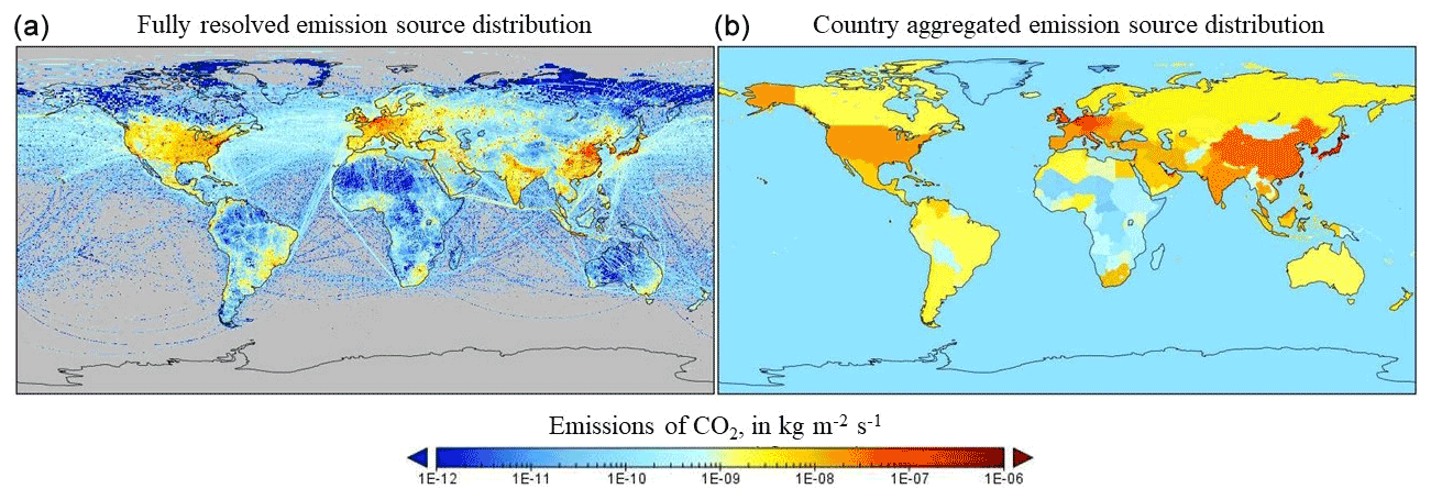
Figure 10Anthropogenic CO2 flux source distribution at ∼ 25 km resolution – fully resolved (a), country aggregated (b).
Model simulations were performed for January 2015 with 3-hourly output. Anthropogenic, fire, ocean, and biogenic fluxes (large-scale model bias mitigated by the biogenic CO2 flux adjustment scheme, BFAS) were considered. For the full model configuration description see McNorton et al. (2020). It was noted that point sources (e.g. power plants, factories) can be easily detected if they comprise a substantial part of countries' total emission budget (e.g. in South Africa). If point sources are distributed homogeneously over the country, and other areal sources are rather high as well, it becomes difficult to detect one extra or missing emitting hotspot (e.g. in Germany). China is a very good example for both cases as its western part has very few hotspots, and they are easy to detect over the low-emitting background. Its eastern part, however, has lots of hotspots and high-emitting areal sources, making it almost impossible to disentangle emissions from a single power plant or factory from the high-emitting background. Differences of several parts per million are detected over multiple regions, highlighting the importance of using high-resolution spatially resolved emissions. With increase in both flux and transport model resolutions, these differences are expected to increase further with steeper atmospheric CO2 gradients.
EDGARv4.3.2 data are open-access and available at http://data.europa.eu/89h/jrc-edgar-edgar_v432_ghg_gridmaps (last access: 29 June 2021, Janssens-Maenhout et al., 2017) and are documented in Janssens-Maenhout et al. (2019). CHE_EDGAR-ECMWF_2015 data are freely available https://doi.org/10.5281/zenodo.3967439 (Choulga et al., 2020) and documented in this paper. The CHE_UNC_APP anthropogenic CO2 emission uncertainty calculation tool is freely available https://doi.org/10.5281/zenodo.5196190 (Choulga et al., 2021) and documented in this paper.
A pre-processor has been created that allows derivation of the upper- and lower-half range of uncertainty grid maps while making use of an appropriate classification of more certain and uncertain sectors. These grid maps allow assessment of the error propagation of country emission budgets following the IPCC 2006 Guidelines for National Greenhouse Gas Inventories. It is a first step in evaluating where to provide more effort in reducing the propagated error budget that can be taken up in any global or regional atmospheric model as a first step. The method has been applied using EDGARv4.3.2_FT2015 and was tested as input to the ECMWF IFS ensemble spread to characterize the carbon dioxide (CO2) atmospheric concentrations' uncertainties in the prototype of the Copernicus CO2 Monitoring and Verification Support Capacity. At the country level the CHE_EDGAR-ECMWF_2015 dataset provides generally larger uncertainty ranges, reduced when more detailed information is available. In summary, using the information uniformly available for all countries, a coherent uncertainty representation is obtained.
The application in the ECMWF IFS Earth system model sheds light on the spatial representativeness of the emissions. While the emission-intensive point sources were checked with reference to their spatial location, the diffuse emission sources are gridded using spatial proxy data. With CHE_EDGAR-ECMWF_2015 implemented in the IFS model it was demonstrated that the choice of the spatial proxy data has a strong influence on the model results. As such, it is proposed that this is analysed in comparison to other datasets, going beyond the evaluation of the probability density of the spatial proxy itself. Contribution of representativeness errors to uncertainties and time correlation will need to be assessed in successive future studies, as foreseen under the Prototype System for a Copernicus CO2 Service (CoCO2) project, following up on the CO2 Human Emissions (CHE) project.
The use of an ensemble technique to estimate CO2 uncertainties is recommended. The optimal number of ensemble members is bound by practical considerations on computational costs. Leutbecher (2018) found a minimum of an 8-member ensemble can mimic some of the skill of larger ensembles, with a 20-member ensemble being a typical value used by several modelling systems and with a 50-member ensemble being a desirable target. Further grouping of anthropogenic emissions into, for example, one to reduce the dimensions of the problem is also possible with the tool CHE_UNC_APP (Choulga et al., 2021).
The estimation of global gridded emissions with their spatially and temporally distributed uncertainties constitute the backbone for atmospheric inversions to estimate anthropogenic emissions from atmospheric concentrations (Pinty et al., 2017). Dedicated satellite missions (e.g. Copernicus anthropogenic CO2 monitoring mission CO2M described in Janssens-Maenhout et al., 2020) are being planned to monitor anthropogenic emissions from space and substantially reduce emission uncertainties. The developments in the emission uncertainty, based on computation of priors presented in this paper, are an important preparatory step for an ensemble-based CO2 monitoring and verification system prototype, such as the one developed within the CHE project.
The supplement related to this article is available online at: https://doi.org/10.5194/essd-13-5311-2021-supplement.
All the authors participated in the uncertainty calculation tool CHE_UNC_APP design and CHE_EDGAR-ECMWF_2015 map generation (methodology, data generation), model experiment set-up, and analysis of the result. Margarita Choulga and Greet Janssens-Maenhout wrote the manuscript with contributions from all the other authors.
The authors declare that they have no conflict of interest.
Publisher's note: Copernicus Publications remains neutral with regard to jurisdictional claims in published maps and institutional affiliations.
The authors thank Glenn Carver (ECMWF) for editorial help and assistance and Vladimir Tupoguz for invaluable support during the preparation of the paper and numerous discussions. Margarita Choulga was funded by the CO2 Human Emissions (CHE) project, which received funding from the European Union's Horizon 2020 research and innovation programme under grant agreement no. 776186, and by the Prototype System for a Copernicus CO2 Service (CoCO2) project, which received funding from the European Union's Horizon 2020 research and innovation programme under grant agreement no. 958927.
This research has been supported by the CO2 Human Emissions (CHE) project (grant no. 776186) and the Prototype System for a Copernicus CO2 Service (CoCO2) project (grant no. 958927).
This paper was edited by David Carlson and reviewed by three anonymous referees.
Agustí-Panareda, A., Massart, S., Chevallier, F., Boussetta, S., Balsamo, G., Beljaars, A., Ciais, P., Deutscher, N. M., Engelen, R., Jones, L., Kivi, R., Paris, J.-D., Peuch, V.-H., Sherlock, V., Vermeulen, A. T., Wennberg, P. O., and Wunch, D.: Forecasting global atmospheric CO2, Atmos. Chem. Phys., 14, 11959–11983, https://doi.org/10.5194/acp-14-11959-2014, 2014.
Agustí-Panareda, A., Diamantakis, M., Massart, S., Chevallier, F., Muñoz-Sabater, J., Barré, J., Curcoll, R., Engelen, R., Langerock, B., Law, R. M., Loh, Z., Morguí, J. A., Parrington, M., Peuch, V.-H., Ramonet, M., Roehl, C., Vermeulen, A. T., Warneke, T., and Wunch, D.: Modelling CO2 weather – why horizontal resolution matters, Atmos. Chem. Phys., 19, 7347–7376, https://doi.org/10.5194/acp-19-7347-2019, 2019.
Amann, M., Bertok, I., Borken-Kleefeld, J., Cofala, J., Heyes, C., Höglund-Isaksson, L., Klimont, Z., Nguyen, B., Posch, M., Rafaj, P., Sandler, R., Schöpp, W., Wagner, F., and Winiwarter, W.: Cost-effective control of air quality and greenhouse gases in Europe: Modelling and policy applications, Environ. Modell. Softw., 26, 1489–1501, 2011.
Andres, R. J., Marland, G., Fung, I., and Matthews, E.: A 1∘ × 1∘ distribution of carbon dioxide emissions from fossil fuel consumption and cement manufacture, 1950–1990, Global Biogeochem. Cy., 10, 419–429, https://doi.org/10.1029/96GB01523, 1996.
Andres, R. J., Boden, T. A., and Marland, G.: Annual Fossil-Fuel CO2 Emissions: Mass of Emissions Gridded by One Degree Latitude by One Degree Longitude, United States: N. p., (NDP-058.2016), ESS-DIVE [data set], https://doi.org/10.3334/CDIAC/ffe.ndp058.2016, 2016.
Andrew, R. M.: A comparison of estimates of global carbon dioxide emissions from fossil carbon sources, Earth Syst. Sci. Data, 12, 1437–1465, https://doi.org/10.5194/essd-12-1437-2020, 2020.
Asefi-Najafabady, S., Rayner, P. J., Gurney, K. R., McRobert, A., Song, Y., Coltin, K., Huang, J., Elvidge, C., Baugh, K.: A multiyear, global gridded fossil fuel CO2 emission data product: Evaluation and analysis of results, J. Geophys. Res.-Atmos., 119, 10.213–10.231, https://doi.org/10.1002/2013JD021296, 2014.
Beamish, B. B. and Vance, W. E.: Greenhouse gas contributions from coal mining in Australia and New Zealand, J. Roy. Soc. New Zeal., 22:2, 153–156, https://doi.org/10.1080/03036758.1992.10420812, 1992.
Bergamaschi, P., Corazza, M., Karstens, U., Athanassiadou, M., Thompson, R. L., Pison, I., Manning, A. J., Bousquet, P., Segers, A., Vermeulen, A. T., Janssens-Maenhout, G., Schmidt, M., Ramonet, M., Meinhardt, F., Aalto, T., Haszpra, L., Moncrieff, J., Popa, M. E., Lowry, D., Steinbacher, M., Jordan, A., O'Doherty, S., Piacentino, S., and Dlugokencky, E.: Top-down estimates of European CH4 and N2O emissions based on four different inverse models, Atmos. Chem. Phys., 15, 715–736, https://doi.org/10.5194/acp-15-715-2015, 2015.
Bond, T. C., Streets, D. G., Yarber, K. F., Nelson, S. M., Woo, J.-H., and Klimont, Z.: A technology-based Global inventory of black and organic carbon emissions from combustion, J. Geophys. Res., 109, D14203, https://doi.org/10.1029/2003JD003697, 2004.
CHE: CO2 Human Emissions (CHE) project official website, available at: https://www.che-project.eu, last access: 29 June 2021.
Chen, H., Huang, Y., Shen, H., Chen, Y., Ru, M., Chen, Y., Lin, N., Su, S., Zhuo, S., Zhong, Q., Wang, X., Liu, J., Li, B., and Tao, S.: Modelling temporal variations in global residential energy consumption and pollutant emissions, Appl. Ener., 184, 0306–2619, 820–829, https://doi.org/10.1016/j.apenergy.2015.10.185, 2016.
Choulga, M., McNorton, J., and Janssens-Maenhout, G.: CHE_EDGAR-ECMWF_2015, Zenodo [data set], https://doi.org/10.5281/zenodo.3967439, 2020.
Choulga, M., Janssens-Maenhout, G., and McNorton, J.: Anthropogenic CO2 emission uncertainty calculation tool CHE_UNC_APP, Zenodo [code], https://doi.org/10.5281/zenodo.5196190, 2021.
Cong, R., Saitō, M., Hirata, R., Ito, A., and Maksyutov, S.: Uncertainty Analysis on Global Greenhouse Gas Inventories from Anthropogenic Sources, in: Proceedings of the 2nd International Conference of Recent Trends in Environmental Science and Engineering (RTESE'18), Niagara Falls, Canada 10-12.06.2018, Paper No. 141, https://doi.org/10.11159/rtese18.141, 2018.
Cong, R., Saitō, M., Hirata, R., Ito, A., and Maksyutov, S.: Uncertainty Analysis on Global Greenhouse Gas Inventories from Anthropogenic Sources, International Journal of Environmental Pollution and Remediation (IJEPR), 7, 1–8, https://doi.org/10.11159/ijepr.2019.001, 2019.
Frey, H. C.: Evaluation of an Approximate Analytical Procedure for Calculating Uncertainty in the Greenhouse Gas Version of the Multi-Scale Motor Vehicle and Equipment Emissions System, Prepared for Office of Transportation and Air Quality, U.S. Environmental Protection Agency, Ann Arbor, MI, 30 May 2003, 2003.
Friedlingstein, P., Jones, M. W., O'Sullivan, M., Andrew, R. M., Hauck, J., Peters, G. P., Peters, W., Pongratz, J., Sitch, S., Le Quéré, C., Bakker, D. C. E., Canadell, J. G., Ciais, P., Jackson, R. B., Anthoni, P., Barbero, L., Bastos, A., Bastrikov, V., Becker, M., Bopp, L., Buitenhuis, E., Chandra, N., Chevallier, F., Chini, L. P., Currie, K. I., Feely, R. A., Gehlen, M., Gilfillan, D., Gkritzalis, T., Goll, D. S., Gruber, N., Gutekunst, S., Harris, I., Haverd, V., Houghton, R. A., Hurtt, G., Ilyina, T., Jain, A. K., Joetzjer, E., Kaplan, J. O., Kato, E., Klein Goldewijk, K., Korsbakken, J. I., Landschützer, P., Lauvset, S. K., Lefèvre, N., Lenton, A., Lienert, S., Lombardozzi, D., Marland, G., McGuire, P. C., Melton, J. R., Metzl, N., Munro, D. R., Nabel, J. E. M. S., Nakaoka, S.-I., Neill, C., Omar, A. M., Ono, T., Peregon, A., Pierrot, D., Poulter, B., Rehder, G., Resplandy, L., Robertson, E., Rödenbeck, C., Séférian, R., Schwinger, J., Smith, N., Tans, P. P., Tian, H., Tilbrook, B., Tubiello, F. N., van der Werf, G. R., Wiltshire, A. J., and Zaehle, S.: Global Carbon Budget 2019, Earth Syst. Sci. Data, 11, 1783–1838, https://doi.org/10.5194/essd-11-1783-2019, 2019.
Hoesly, R. M., Smith, S. J., Feng, L., Klimont, Z., Janssens-Maenhout, G., Pitkanen, T., Seibert, J. J., Vu, L., Andres, R. J., Bolt, R. M., Bond, T. C., Dawidowski, L., Kholod, N., Kurokawa, J.-I., Li, M., Liu, L., Lu, Z., Moura, M. C. P., O'Rourke, P. R., and Zhang, Q.: Historical (1750–2014) anthropogenic emissions of reactive gases and aerosols from the Community Emissions Data System (CEDS), Geosci. Model Dev., 11, 369–408, https://doi.org/10.5194/gmd-11-369-2018, 2018.
IPCC: 2006 IPCC Guidelines for National Greenhouse Gas Inventories, edited by: Eggleston, S., Buendia, L., Miwa, K., Ngara, T., and Tanabe, K., IPCC-TSU NGGIP, IGES, Hayama, Japan, available at: https://www.ipcc-nggip.iges.or.jp/public/2006gl/index.html (last access: 29 June 2021), 2006.
IPCC: 2019 Refinement to the 2006 IPCC Guidelines for National Greenhouse Gas Inventories, Calvo Buendia, E., Guendehou, S., Limmeechokchai, B., Pipatti, R., Rojas, Y., Sturgiss, R., Tanabe, K., Wirth, T., Romano, D., Witi, J., Garg, A., Weitz, M. M., Bofeng, C., Ottinger, D. A., Dong, H., MacDonald, J. D., Ogle, S. M., Theoto Rocha, M., Sanz Sanchez, M. J., Bartram, D. M., and Towprayoon, S. (authors), edited by: Gomez, D. and Irving, W., Vol. 1. Ch. 8, Task Force on National Greenhouse Gas Inventories (TFI), IPCC’s 49th Session, 12 May 2019, Kyoto, Japan, 2019.
Janssens-Maenhout, G., Crippa, M., Guizzardi, D., Muntean, M., and Schaaf, E.: Emissions Database for Global Atmospheric Research, version v4.3.2 part I Greenhouse gases (gridmaps), European Commission, Joint Research Centre (JRC) [data set], available at: http://data.europa.eu/89h/jrc-edgar-edgar_v432_ghg_gridmaps (last access: 29 June 2021), 2017.
Janssens-Maenhout, G., Crippa, M., Guizzardi, D., Muntean, M., Schaaf, E., Dentener, F., Bergamaschi, P., Pagliari, V., Olivier, J. G. J., Peters, J. A. H. W., van Aardenne, J. A., Monni, S., Doering, U., Petrescu, A. M. R., Solazzo, E., and Oreggioni, G. D.: EDGAR v4.3.2 Global Atlas of the three major greenhouse gas emissions for the period 1970–2012, Earth Syst. Sci. Data, 11, 959–1002, https://doi.org/10.5194/essd-11-959-2019, 2019.
Janssens-Maenhout, G., Pinty, B., Dowell, M., Zunker, H., Andersson, E., Balsamo, G., Bézy, J.-L., Brunhes, T., Bösch, H., Bojkov, B., Brunner, D., Buchwitz, M., Crisp, D., Ciais, P., Counet, P., Dee, D., Denier van der Gon, H., Dolman, H., Drinkwater, M., Dubovik, O., Engelen, R., Fehr, T., Fernandez, V., Heimann, M., Holmlund, K., Houseling, S., Husband, R., Juvyns, O., Kentarchos, A.,. Landgraf, J., Lang, R., Löscher, A., Marshall, J., Meijer, Y., Nakajima, M., Palmer, P., Peylin, P., Rayner, P., Scholze, M., Sierk, B., and Veefkind, P.: Towards an operational anthropogenic CO2 emissions monitoring and verification support capacity, B. Am. Meteorol. Soc., 101, E1439–E1451, https://doi.org/10.1175/BAMS-D-19-0017.1, 2020.
Jones, M. W., Andrew, R. M., Peters, G. P., Janssens-Maenhout, G., De-Gol, A. J., Ciais, P., Patra, P. K., Chevallier, F., and Le Quéré, C.: Gridded fossil CO2 emissions and related O2 combustion consistent with national inventories 1959–2018, Sci. Data, 8, 2, https://doi.org/10.1038/s41597-020-00779-6, 2021.
Kuenen, J. J. P., Visschedijk, A. J. H., Jozwicka, M., and Denier van der Gon, H. A. C.: TNO-MACC_II emission inventory; a multi-year (2003–2009) consistent high-resolution European emission inventory for air quality modelling, Atmos. Chem. Phys., 14, 10963–10976, https://doi.org/10.5194/acp-14-10963-2014, 2014.
Liu, Z., Guan, D., Wei, W., Davis, S. J., Ciais, P., Bai, J., Peng, S., Zhang, Q., Hubacek, K., Marland, G., Andres, R. J., Crawford-Brown, D., Lin, J., Zhao, H., Hong, C., Boden, T. A., Feng, K., Peters, G. P., Xi, F., Liu, J., Li, Y., Zhao, Y., Zeng, N., and He, K.: Reduced carbon emission estimates from fossil fuel combustion and cement production in China, Nature, 524, 7565, 335–338, https://doi.org/10.1038/nature14677, 2015.
Leutbecher, M.: Ensemble size: How suboptimal is less than infinity?, Q. J. Roy. Meteor. Soc., 145, 107–128, https://doi.org/10.1002/qj.3387, 2018.
Marland, G., Pielke Sr., R., Apps, M., Avissar, R., Betts, R., Davis, K., Frumhoff, P., Jackson, S., Joyce, L., Kauppi, P., Katzenberger, J., Macdicken, K., Neilson, R., Niles, J., Niyogi, D., Norby, R., Pena, N., Sampson, N., and Xue, Y.: The climatic impacts of land surface change and carbon management, and the implications for climate-change mitigation policy, Clim. Policy, 3, 149–157, https://doi.org/10.3763/cpol.2003.0318, 2003.
Marland, G., Boden, T. A., and Andres, R. J.: Global, regional, and national fossil fuel CO2 emissions, in: Trends: A Compendium of Data on Global Change, US Department of Energy, Carbon Dioxide Information Analysis Center, Oak Ridge National Laboratory, Oak Ridge, Tennessee, USA, 2006.
McNorton, J. R., Bousserez, N., Agustí-Panareda, A., Balsamo, G., Choulga, M., Dawson, A., Engelen, R., Kipling, Z., and Lang, S.: Representing model uncertainty for global atmospheric CO2 flux inversions using ECMWF-IFS-46R1, Geosci. Model Dev., 13, 2297–2313, https://doi.org/10.5194/gmd-13-2297-2020, 2020.
Oda, T. and Maksyutov, S.: A very high-resolution (1 km × 1 km) global fossil fuel CO2 emission inventory derived using a point source database and satellite observations of nighttime lights, Atmos. Chem. Phys., 11, 543–556, https://doi.org/10.5194/acp-11-543-2011, 2011.
Oda, T., Maksyutov, S., and Andres, R. J.: The Open-source Data Inventory for Anthropogenic CO2, version 2016 (ODIAC2016): a global monthly fossil fuel CO2 gridded emissions data product for tracer transport simulations and surface flux inversions, Earth Syst. Sci. Data, 10, 87–107, https://doi.org/10.5194/essd-10-87-2018, 2018.
Oda, T., Bun, R., Kinakh, V., Topylko, P., Halushchak, M., Marland, G., Lauvaux, T., Jonas, M., Maksyutov, S., Nahorski, Z., Lesiv, M., Danylo, O., and Horabik-Pyzel, J.: Errors and uncertainties in a gridded carbon dioxide emissions inventory, Mitig. Adapt. Strat. Gl., 24, 1007–1050, https://doi.org/10.1007/s11027-019-09877-2, 2019.
ODIAC: ODIAC Fossil Fuel CO2 Emissions Dataset, ODIAC [data set], https://doi.org/10.17595/20170411.001, 2021.
Olivier, J. G. J. and Janssens-Maenhout, G.: CO2 Emissions from Fuel Combustion – 2016 Edition, IEA CO2 report 2016, Part III, Greenhouse-Gas Emissions, OECD – IEA, ISBN 9789264258563, EU Science Hub, https://doi.org/10.1787/co2_fuel-2016-en, 2016a.
Olivier, J. G. J., Janssens-Maenhout, G., Muntean, M., and Peters, J. A. H. W.: Trends in global CO2 emissions: 2016 report, PBL Netherlands Environmental Assessment Agency, The Hague, the Netherlands, PBL publication number: 2315, European Commission, Joint Research Centre, Directorate Energy, Transport & Climate, JRC Science for Policy Report: 103428, 1–86, available at: https://www.pbl.nl/sites/default/files/downloads/pbl-2016-trends-in-global-co2-emisions-2016-report-2315_4.pdf (last access: 29 June 2021), 2016b.
Petrescu, A. M. R., Peters, G. P., Janssens-Maenhout, G., Ciais, P., Tubiello, F. N., Grassi, G., Nabuurs, G.-J., Leip, A., Carmona-Garcia, G., Winiwarter, W., Höglund-Isaksson, L., Günther, D., Solazzo, E., Kiesow, A., Bastos, A., Pongratz, J., Nabel, J. E. M. S., Conchedda, G., Pilli, R., Andrew, R. M., Schelhaas, M.-J., and Dolman, A. J.: European anthropogenic AFOLU greenhouse gas emissions: a review and benchmark data, Earth Syst. Sci. Data, 12, 961–1001, https://doi.org/10.5194/essd-12-961-2020, 2020.
Pinty, B., Janssens-Maenhout, G., Dowell, M., Zunker, H., Brunhes, T., Ciais, P., Dee, D., Denier van der Gon, H., Dolman, H., Drinkwater, M., Engelen, R., Heimann, M., Holmlund, K., Husband, R., Kentarchos, A., Meijer, Y., Palmer, P., and Scholze, M.: An operational anthropogenic CO2 emissions monitoring & verification support capacity – Baseline requirements, Model components and functional architecture, European Commission Joint Research Centre, Publications Office of the European Union, Luxembourg, JRC107499, EUR 28736 EN, ISBN 978-92-79-72101-4, https://doi.org/10.2760/08644, 2017.
Super, I., Dellaert, S. N. C., Visschedijk, A. J. H., and Denier van der Gon, H. A. C.: Uncertainty analysis of a European high-resolution emission inventory of CO2 and CO to support inverse modelling and network design, Atmos. Chem. Phys., 20, 1795–1816, https://doi.org/10.5194/acp-20-1795-2020, 2020.
Wang, R., Tao, S., Ciais, P., Shen, H. Z., Huang, Y., Chen, H., Shen, G. F., Wang, B., Li, W., Zhang, Y. Y., Lu, Y., Zhu, D., Chen, Y. C., Liu, X. P., Wang, W. T., Wang, X. L., Liu, W. X., Li, B. G., and Piao, S. L.: High-resolution mapping of combustion processes and implications for CO2 emissions, Atmos. Chem. Phys., 13, 5189–5203, https://doi.org/10.5194/acp-13-5189-2013, 2013.
Often, emission budgets are provided not per IPCC (2006) activity but for several activities together (usually due to measuring or reporting limitations), for which the user then needs to assume a lump sum activity, emission factor, and uncertainties in those.
CHE stands for the CO2 Human Emissions project (CHE, 2021).