Description of a global marine particulate organic carbon-13 isotope data set

Marine particulate organic carbon stable isotope ratios (δ¹³C_POC) provide insights into understanding carbon cycling through the atmosphere, ocean and biosphere. They have for example been used to trace the input of anthropogenic carbon in the marine ecosystem due to the distinct isotopically light signature of anthropogenic emissions. However, δ¹³C_POC is also significantly altered during photosynthesis by phytoplankton, which complicates its interpretation. For such purposes, robust spatio-temporal coverage of δ¹³C_POC observations is essential. We collected all such available data sets and merged and homogenized them to provide the largest available marine δ¹³C_POC data set (https://doi.org/10.1594/PANGAEA.929931; Verwega et al., 2021). The data set consists of 4732 data points covering all major ocean basins beginning in the 1960s. We describe the compiled raw data, compare different observational methods, and provide key insights in the temporal and spatial distribution that is consistent with previously observed large-scale patterns. The main different sample collection methods (bottle, intake, net, trap) are generally consistent with each other when comparing within regions. An analysis of 1990s median δ¹³C_POC values in a meridional section across the best-covered Atlantic Ocean shows relatively high values ($\ge -\mathrm{22}$ ‰) in the low latitudes (<30^∘) trending towards lower values in the Arctic Ocean ($\sim -\mathrm{24}$ ‰) and Southern Ocean ($\le -\mathrm{28}$ ‰). The temporal trend since the 1960s shows a decrease in the median δ¹³C_POC by more than 3 ‰ in all basins except for the Southern Ocean, which shows a weaker trend but contains relatively poor multi-decadal coverage.

1 Introduction

Carbon is an essential element for life, and it regulates climate via its atmospheric form CO₂, a long-living greenhouse gas. Understanding carbon cycling is fundamental to reliably projecting changes in the Earth's future climate. Carbon is subject to transformation and cycling throughout the ocean, land and atmosphere. It is a major part of organic matter of all living organisms which can both consume (e.g., photosynthesis) and produce (e.g., respiration) inorganic carbon. Besides the natural cycling processes, the total amount and distribution of carbon is strongly perturbed by human activity caused by industrialization, most notably due to fossil fuel emissions, deforestation, farming, cement production and other industrial processes. Anthropogenic CO₂ emissions are one of the main driving forces of modern climate change which is likely to continue in the future (IPCC, 2013). Only about 60 % of anthropogenic CO₂ emissions have been compensated for by natural sinks, including the dissolution of inorganic carbon in the ocean. This means the atmosphere has already been enriched with anthropogenic carbon by about 880 Gt CO₂ since 1750 (IPCC, 2014), which is driving the increase in global temperature levels. The ocean serves as an important buffer as it absorbs a significant amount of anthropogenic carbon, with the ocean interior being the largest readily exchangeable reservoir of carbon in the Earth system.

Marine phytoplankton convert dissolved inorganic carbon (e.g., aqueous CO₂) into organic carbon via photosynthesis in the euphotic surface layer. This organic carbon forms the base of the food web for higher tropic levels in marine ecosystems. Some particulate organic carbon (POC) sinks down to ocean depths, where it either is respired back to dissolved inorganic carbon by heterotrophic organisms or becomes buried in ocean sediments (Suess, 1980). This process is known as the soft-tissue biological carbon pump, an important mechanism for sequestering carbon to the deep ocean from the atmosphere (Volk and Hoffert, 1985; Banse, 1990; McConnaughey and McRoy, 1979). Since the deep ocean has a residence time of about a millennium, it is a key carbon reservoir influencing long-term climate change.

Carbon isotopes provide additional insights into the cycling of carbon in the Earth system (Zeebe and Wolf-Gladrow, 2001). The element carbon exists in two naturally occurring stable isotopes, ¹²C and ¹³C, with abundances of around 98.9 % and 1.1 %, respectively. Knowledge of their pathways through carbon reservoirs can support deeper understanding of carbon transfer and can help identify carbon sources with different isotopic ratios (Rounick and Winterbourn, 1986). Relative abundances of carbon isotopes are usually given in δ notation, which is based on the carbon isotope ratio $\frac{{}^{\mathrm{13}}\text{C}}{{}^{\mathrm{12}}\text{C}}$, standardized and given in parts per thousands as

$$\begin{array}{}\text{(1)}& {\mathit{\delta }}^{\mathrm{13}}\text{C}=\left({\displaystyle \frac{\frac{{}^{\mathrm{13}}\text{C}}{{}^{\mathrm{12}}\text{C}}}{R_{\mathrm{std}}}}-\mathrm{1}\right).\end{array}$$

The constant R_std=0.0112372 is a standard ratio, originally referring to the calcareous fossil Pee Dee Belemnite. The values ¹²C and ¹³C are the absolute concentrations of the individual isotopes (Hayes, 2004).

Distributed within the carbon cycle, the fractionation of δ¹³C is influenced by biological and thermodynamic processes (Gruber et al., 1999). Air–sea gas exchange plays a dominant role at the ocean surface. Phytoplankton photosynthesis and POC remineralization increase their influence in the ocean interior (Gruber et al., 1999; Morée et al., 2018). The processes are dependent on circulation and temperature, and thus their individual influence varies with geographic location (Gruber et al., 1999; Schmittner et al., 2013).

Phytoplankton preferentially incorporate (i.e., fractionate) the lighter ¹²C carbon isotope into its organic matter. This fractionation causes phytoplankton organic δ¹³C to be 10 ‰ to 25 ‰ lower than that of inorganic δ¹³C, which depends on a variety of environmental, ecological and physiological conditions (e.g., Popp et al., 1989, 1998; Rau et al., 1989, 1996). The main factors that control phytoplankton fractionation are concentrations of CO₂(aq), species-specific effects enforced by the phytoplankton composition and the cellular growth rate, although uncertainties remain regarding the quantification of the specific processes and mechanisms that cause variations in phytoplankton fractionation (e.g., Fry, 1996; Laws et al., 1995; Popp et al., 1998; Bidigare et al., 1997; Cassar et al., 2006).

δ¹³C_POC provides insights into physical and biological carbon cycle processes in the ocean (e.g., Fry and Sherr, 1989). It helps to diagnose carbon pathways from the atmosphere to the deep ocean including the biological carbon pump (e.g., Jasper and Hayes, 1990; Popp et al., 1989; Freeman and Hayes, 1992) and assists reconstruction of oceanic carbon cycling and even plankton cell size and community structure (e.g., Tuerena et al., 2019; Lorrain et al., 2020). For example, anthropogenic carbon emissions have a distinctly low δ¹³C content, making δ¹³C a useful property for tracing anthropogenic carbon throughout the Earth system (Eide et al., 2017; Levin et al., 1989; Ndeye et al., 2017). Atmospheric δ¹³C${}_{{\mathrm{CO}}_{\mathrm{2}}}$ has decreased from −6.5 ‰ in preindustrial times to −8.4 ‰ presently (Rubino et al., 2013). The measurable decrease due to anthropogenic fossil carbon emissions is known as the Suess effect (Keeling, 1979), which enters the ocean via air–sea gas exchange. However, changes in marine δ¹³C_POC are also significantly influenced by changes in phytoplankton fractionation due to other anthropogenic controls. For example increasing CO₂(aq) concentrations increase surface δ¹³C fractionation (Young et al., 2013) and changes in phytoplankton composition and temperature influence phytoplankton growth rates and δ¹³C fractionation over the air–sea interface (Zhang et al., 1995). But determination of the driving processes(es) of δ¹³C_POC spatial and temporal trends remains a challenge. We also stress that all of these processes are sensitive to temperature changes which adds additional complexity to understanding how fractionation may change in space and time. A better understanding of the contributions from all of these effects requires a robust global data set of δ¹³C_POC.

Theoretical projection and understanding of changes associated with δ¹³C_POC can be executed by models of different scales, which include δ¹³C_POC circulation. Earth system models serve to simulate and test hypotheses in different scenarios as unbiased assessments (e.g., IPCC, 2014) and may support future decision-making. Besides resolving the mass flux of carbon, many models also simulate stable carbon isotopes (e.g., Schmittner and Somes, 2016; Buchanan et al., 2019; Hofmann et al., 2000; Jahn et al., 2015; Tagliabue and Bopp, 2008; Morée et al., 2018; Magozzi et al., 2017). For reliable calibrations and validations of such processed-based mechanistic models, a spatially and temporally comprehensive data set is essential. This additional constraint provided by marine δ¹³C_POC assists the reconstruction of oceanic carbon cycling including how much anthropogenic carbon is entering marine ecosystems and being exported to the deep ocean. But until today, there has been a lack of suitable data sets as constraints. This results in large and mostly unknown uncertainties in model results.

Data sets of marine δ¹³C_POC improve our understanding of marine carbon cycling by providing another independent constraint. Recent model approaches support long-term past climate projections (Tjiputra et al., 2020) and assess estimations of the Suess effect (Liu et al., 2021). To date, numerous individual δ¹³C_POC data sets exist, while the number of accessible, merged data sets is lacking. Existing merged data sets contain data from several sources but have often been focused on a specific region or process (e.g., Goericke, 1994; Tuerena et al., 2019). Individual data sets are usually collected during a specific cruise or time series station and are often neglected since they contain relatively few data. Such data sets can easily be accessed on data platforms such as PANGAEA and, when combined, they can represent an important and significant source of data.

In this study, we provide a novel merged seawater δ¹³C_POC data product (Verwega et al., 2021) that – to our knowledge – contains the most expansive spatio-temporal coverage to date. It contains all available δ¹³C_POC seawater data from PANGAEA and the merged data sets by Goericke (1994), Tuerena et al. (2019) and Young et al. (2013), as well as unpublished data from different cruises by Anne Lorrain. No data were excluded, even if sampled at extreme locations (e.g.,  trenches, hydrothermal vents). The metadata comprise information about the sampling location, time, depth and method as well as the original source, which makes original raw data values, methods, and further technical description easily accessible. Provided data files are Network Common Data Form (NetCDF) files interpolated onto two different global grids and a csv file that includes the data and their anomalies with respect to their overall mean together with all corresponding available meta-information.

The paper is structured as follows: we provide a brief overview of δ¹³C_POC data acquisition in Sect. 2 and their compilation and metadata in Sect. 3. The characteristics of the collected δ¹³C_POC data are shown in Sect. 4. We present their spatial distribution in Sect. 5 and temporal distribution in Sect. 6. Lastly, we provide a short summary and concluding remarks.

2 Data acquisition

The data set includes 4732 entries for δ¹³C_POC from 185 different sources and ranges from the 1960s to the 2010s. In addition to many data sets from the data platform PANGAEA, we included unpublished data provided by Anne Lorrain and the data products from Tuerena et al. (2019), Goericke (1994) and Young et al. (2013). The adjustments that we conducted are described in the following.

2.1 Data sources

As a basis of our data set, we chose the 1990s data collection by Goericke (1994). This was established to investigate variations in δ¹³C_POC with temperature and latitude. The δ¹³C_POC sample data and measurements were conducted by investigating zooplankton, net plankton or particulate organic matter. We cross-checked and extended this data set by looking up all available primary sources. Goericke (1994) originally included 476 δ¹³C_POC data points from 17 contributions. The largest contributions came from Fischer (1989) with 107 entries, Fontugne et al. (1991) with 97, and Fontugne and Duplessy (1981, 1978) with 78. Large extensions were possible, e.g., in the Fischer (1989) and Eadie and Jeffrey (1973) data sets, incorporating more than 70 additional data points from these primary sources. With this extension, we could increase the data set to 626 data points for δ¹³C_POC.

We collected most data from the PANGAEA data platform, an open-access online library archiving and providing geo-referenced Earth system data, hosted and monitored by the Alfred-Wegener-Institut (2020) – Helmholtz Centre for Polar and Marine Research (AWI) – and the Center for Marine Environmental Sciences, University of Bremen (MARUM). With the data made available therein, we could further extend the data set by an additional ∼ 3500 measurements of δ¹³C_POC. Most δ¹³C_POC data from PANGAEA are associated with samples collected during the Joint Global Ocean Flux Study (JGOFS, 2020), with more than 2000 δ¹³C_POC data points. Additionally, 529 samples are contributions by the Antarctic Environment and Southern Ocean Process Study (AESOPS, 2020), 342 are by the Archive of Ocean Data (EurOBIS Data Management Team, 2020) and 279 are by the SFB313 research project (Thiede et al., 1988).

Other collected data were provided by Robyn Tuerena and Anne Lorrain. Robyn Tuerena provided a data contribution coming from the data set mentioned in Tuerena et al. (2019), which we will refer to as the Tuerena data set. This contains 595 data points including 501 from Young et al. (2013) and covers samples within the euphotic zone and an observation time frame of 1964–2012. Moreover, we included 69 unpublished data points provided by Anne Lorrain, covering the years 2012–2015 and sampled during the cruises CASSIOPEE, PANDORA, OUTPACE, NECTALIS-3, NECTALIS-4 and KH-13. We refer to this data set as the Lorrain data set.

A recent collection of 303 measurements of δ¹³C_POC has been provided by Close and Henderson (2020), largely based on data gathered from individual publications referenced therein. Since our analyses originally relied on data sources that differed from those of Close and Henderson (2020), we find our collection to be as yet incomplete. Especially measurements from national databases might provide a huge future benefit.

2.2 Adjustments made

All data were taken with as many details as possible from the sources and have been reshaped to fit the structure of the data set. No rounding or cutoff of detailed data was made. Spatial coordinates originally given as depth intervals were replaced by their respective midpoints. Time intervals were not changed in this way. If they contained just 1 month or year, this was included; otherwise the time information was omitted. Sample depth given as “surface” was denoted as 1 m. Longitude values were converted to the format $[-\mathrm{180}{}^{\circ },\mathrm{180}{}^{\circ }]$ by the transformation

$$\begin{array}{}\text{(2)}& {\mathrm{Long}}_{\mathrm{new}}=\left\{\begin{array}{ll}{\mathrm{Long}}_{\mathrm{old}}-\mathrm{360}{}^{\circ }& \text{for all }{\mathrm{Long}}_{\mathrm{old}}\in \left(\mathrm{180}{}^{\circ },\mathrm{360}{}^{\circ }\right]\\ {\mathrm{Long}}_{\mathrm{old}}& \text{otherwise.}\end{array}\right.\end{array}$$

Wherever possible the data were taken from their original publication. Changes made to the data by Goericke (1994) are described in Table 1 and changes to all other data in Table 2. The complete structure is presented in Table 3.

Degens et al. (1968)Goericke (1994)Eadie and Jeffrey (1973)Goericke (1994)Fischer (1989)Goericke (1994)Fontugne and Duplessy (1978)Goericke (1994)Fontugne and Duplessy (1981)Goericke (1994)Francois et al. (1993)Goericke (1994)Goericke (1994)Sacket et al. (1965)Goericke (1994)Saupe et al. (1989)Goericke (1994)Wada et al. (1987)Goericke (1994)Eadie and Jeffrey (1973)Goericke (1994)Goericke (1994)Fischer (1989)Goericke (1994)Goericke (1994)Fontugne and Duplessy (1978)Goericke (1994)Goericke (1994)Fontugne and Duplessy (1981)Goericke (1994)Goericke (1994)Francois et al. (1993)Goericke (1994)Goericke (1994)Sacket et al. (1965)Goericke (1994)Goericke (1994)Eadie and Jeffrey (1973)Goericke (1994)Fischer (1989)Goericke (1994)Sacket et al. (1965)Goericke (1994)Wada et al. (1987)Goericke (1994)Fischer (1989)Goericke (1994)Goericke (1994)Fontugne and Duplessy (1978)Goericke (1994)Goericke (1994)Fontugne and Duplessy (1981)Goericke (1994)Goericke (1994)Fischer (1989)Goericke (1994)Goericke (1994)Fontugne and Duplessy (1981)Goericke (1994)Goericke (1994)Francois et al. (1993)Goericke (1994)Goericke (1994)Sacket et al. (1965)Goericke (1994)Goericke (1994)Fischer (1989)Goericke (1994)Fontugne and Duplessy (1978)Goericke (1994)

Table 1 Changes that were introduced into data taken from Goericke (1994): the first column names the publication or author of the primary data set. The second column lists in which part of the data we applied changes. The third and fourth columns show what these changes were, and the last column gives the reason for this.

^∗ The original source was not available, but we highly suspected an error in the coordinates that interchanged east and west.

Trull and Armand (2013a)Trull and Armand (2001)Trull and Armand (2013b)Trull and Armand (2001)Chang et al. (2013)MacKenzie et al. (2019)Voss and von Bodungen (2003)De Jonge et al. (2015a)De Jonge et al. (2015b)

Table 2 Changes made in other data: this table's structure is equivalent that of to Table 1. It refers to all changes made in general and any data other than the Goericke (1994) data.

¹ By arithmetic mean. ² Only for sample durations entirely within an explicit month and year, otherwise information on time frames has been discarded. ³ We applied Eq. (2).

Table 3 Available data and meta-information: the columns of the raw data set correspond to the provided data and meta-information. Their names are given in the first column of this table. The second holds a short description of their content and the third their ranges of values. In the final column we give how well this data kind is covered relative to the size of the full data set.

¹ Ratio of available entries relative to the full number of data points. ² Wherever possible, this includes: author(s), year, title, journal name, full, number, issue, pages and DOI. ³ Primary source was not available in every case as a reference. A note, where the data were taken is included in this case. ⁴ With as many decimal places as available. ⁵ Rounded to two decimal places. ⁶ Here, abundance is given relative to the full number of sediment trap samples.

Most data listed in the Goericke (1994) data set could be gathered from the original publications directly. Some data are not accessible from an original source, including those data labeled as “Harrison”, “Hobson” and “Schell”, which were included as unpublished data by personal communication in Goericke (1994). Also, we could not identify the original data sources of “Voss (1991)” and “Sackett et al. (1966)”. Data from these sources are used as provided by Goericke (1994). All other data could be directly compared with and linked to their origin. According to Table 3 we complemented the data with the month, year, depth, sample method, cruise, trap duration and references wherever available. Special notes given in Goericke (1994) were conserved in our “project/cruise”-named meta-information. Rounded values were adjusted to their source values as well as data with interchanged longitudinal information, which is shown in detail in Table 1.

In two cases we identified multiple δ¹³C_POC data sets from a single event (time, place, investigator) where the data had been subject to different stages of processing or different types of measurement: in Westerhausen and Sarnthein (2003), we chose the “mass spectrometer” data set because this was the originally measured one. In Trull and Armand (2013a, b), we used the “blank corrections” data set of δ¹³C, since this set of δ¹³C_org values is recommended to be considered (Trull and Armand, 2001).

The primary source of the Tuerena and Lorrain data was mentioned in our data set in the project/cruise column. In the data set from Tuerena et al. (2019), this was originally labeled as “source” and in the Lorrain data set as “campaign”. In both data sets the longitude was converted to $[-\mathrm{180}{}^{\circ },\mathrm{180}{}^{\circ }]$ from a $[\mathrm{0}{}^{\circ },\mathrm{360}{}^{\circ }]$ format by Eq. (2). In the data of MacKenzie et al. (2019) we deleted a typo where the depth value was set equal to the negative longitude value. We disregarded the trap duration given in Voss and von Bodungen (2003), which was given as the negative value −1.

3 Content and structure of the data set

The data collection is made available in files of raw and interpolated values (Verwega et al., 2021). The raw data are in a csv file that includes the δ¹³C_POC measurements, their anomalies with respect to their mean and all available meta-information. The interpolated data are provided as NetCDF files on two different global grids: a $\mathrm{1.8}{}^{\circ }\times \mathrm{3.6}{}^{\circ }$ resolution and 19 depth layers from a model that simulates δ¹³C_POC (e.g., Schmittner and Somes, 2016), in the following referred to as the UVic grid, and the $\mathrm{1}{}^{\circ }\times \mathrm{1}{}^{\circ }$ resolution and 102-depth-layer grid of the World Ocean Atlas (Garcia et al., 2018), in the following referred to as the WOA grid. Interpolation required the availability of the full spatial information (latitude, longitude and depth) of included δ¹³C_POC data to locate them on the grid.

On the WOA grid we provide 13 NetCDF files containing only data with full spatio-temporal metadata: one averages all observations from each year together, each year accounting for a time increment on the time axis, and the other 12 files average only observations from an individual month with again each year accounting for a time increment on the time axis. These files provide a variety of analysis opportunities but also limited the content of δ¹³C_POC data.

On the UVic grid we provide seven individual NetCDF files: six of them each represent one of the decades from the 1960s to the 2010s containing all data which were able to be assigned to their respective decade. One file contains all available δ¹³C_POC data completely independent of their measurement time. This individual provision of data on a decadal and overall timescale increases the fraction of usable δ¹³C_POC data for the following analyses.

3.1 Raw data file

The csv-format data file includes δ¹³C_POC measurements, anomalies and meta-information in its columns. A full description of the content, value range and coverage of the individual columns is given in Table 3. Anomalies of δ¹³C_POC were calculated, based on the arithmetic mean of the full data collection. The mean was calculated, rounded to two digits after the floating point and used as

$$\begin{array}{}\text{(3)}& {\mathrm{mean}}_{{\mathit{\delta }}^{\mathrm{13}}{\text{C}}_{\mathrm{POC}}}=-\mathrm{23.96}\mathrm{‰}.\end{array}$$

Anomalies contain all the relevant information with respect to the variability in the δ¹³C_POC data in space and time. This way it becomes easier to analyze bias information separately, e.g., during the first steps of model calibration.

The reference includes the citations in as much detail as possible. Wherever available, this is taken from the original source. Otherwise, we tried to include the author, title, publication year and platform, and DOI. For unpublished data like Harrison's (unpublished data, quoted from Goericke, 1994) from the Goericke (1994) data set or those included by the co-authors, we specified from where we took the data.

Coordinates are given in decimal degrees over $[-\mathrm{90}{}^{\circ },\mathrm{90}{}^{\circ }]\times [-\mathrm{180}{}^{\circ },\mathrm{180}{}^{\circ }]$. The sample depth is given in meters measured positively from the ocean surface downwards. Data published as measured at 0 m were included as this, while no surface microlayer measurements were included. The month and year were used to describe the sample date; specific days are neglected.

Anomalies of δ¹³C_POC are given in the δ ratio described in Eq. (1). A sample method was added, wherever available. Any special sampling circumstances were given in the “Note” column. Activity duration of sediment traps was denoted in the last column.

The “Origin” columns listed the associated project or cruise or author note. Some samples were given with multiple project connections; all of them were given in this column.

3.2 Interpolated data sets

The interpolated δ¹³C_POC data are available as NetCDF files on two global grids with different resolutions. NetCDF files are machine-independent and support the creation, accessing and sharing of array-oriented scientific data. On the UVic grid, we provide seven different files, each of them independent of time and averaged over the available spatial information. Six of them contain an individual decade each (from the 1960s through the 2010s). The seventh file comprises a combined set of all interpolated δ¹³C_POC data. On the WOA grid, we provide 13 files including all δ¹³C_POC measurements with complete spatial–temporal information, averaged across time and space.

One major aim of this work is to support reliable validation and calibration of δ¹³C_POC-simulating models. Hence, we chose the grid of the UVic model version 2.9, as used, e.g., in Schmittner and Somes (2016). Horizontally, it consists of 100×100 cells with a resolution of $\mathrm{1.8}{}^{\circ }\times \mathrm{3.6}{}^{\circ }$, arranged from 0 to 360^∘ in longitude (LONG) and −90 to 90^∘ in latitude (LAT). Vertically, it is split up into 19 vertical layers (DEPTH), decreasing in resolution with depth. The two uppermost layers reach down to depths of 50 and 130 m, respectively, and they are supposed to comprise the upper ocean's euphotic zone.

The WOA grid is based on the $\mathrm{1}{}^{\circ }\times \mathrm{1}{}^{\circ }$ grid of the World Ocean Atlas (Garcia et al., 2018). It has a horizontal resolution of 360 arranged from −180 to 180^∘ in the longitude (LONG) and 180 arranged from −90 to 90^∘ in the latitude (LAT) direction. Vertically, it is split up into 102 layers (DEPTH). The time axis (TIME) increases in increments for each year from 1964 to 2015 by 1 and has a size of 52. This interpolation includes only δ¹³C_POC data with full spatio-temporal metadata coverage; i.e., additionally to latitude, longitude and depth, we also required and included year and month information.

Ferret scripts were used for the interpolations. These averaged the irregularly measured data points within the ocean grid to one single data point representing each covered grid cell. The interpolation function SCAT2GRIDGAUSS by NOAA's Pacific Marine Environmental Laboratory (2020) performed the spatial averaging under PyFerret v7.5. Calculations in this function are based on a work by Kessler and McCreary (1992) and can be summarized as follows: let $(x_{\mathrm{1}},y_{\mathrm{1}}),\mathrm{\dots },(x_n,y_n)\subseteq {\mathbb{R}}^{\mathrm{2}}$ be an equidistant grid and $(\stackrel{\mathrm{̃}}{x_{\mathrm{1}}},\stackrel{\mathrm{̃}}{y_{\mathrm{1}}}),\mathrm{\dots },(\stackrel{\mathrm{̃}}{x_m},\stackrel{\mathrm{̃}}{y_m})\subseteq {\mathbb{R}}^{\mathrm{2}}$ be irregular measurement locations of a real tracer $D_j,j\in \mathit{\{}\mathrm{1},\mathrm{\dots },m\mathit{\}}$. Then the value D_i∈ℝ at grid point $(x_i,y_i),i\in \mathit{\{}\mathrm{1},\mathrm{\dots },n\mathit{\}}$ becomes interpolated as

$$\begin{array}{}\text{(4)}& D_i:={\displaystyle \frac{{\sum }_{j=\mathrm{1}}^m{D}_j{W}_{i,j}}{{\sum }_{j=\mathrm{1}}^m{W}_{i,j}}},\end{array}$$

where

$$\begin{array}{}\text{(5)}& W_{i,j}:=\left\{\begin{array}{ll}\mathrm{0};& {\mathit{\tau }}_{i,j}<e^{-CX}\\ \mathrm{0};& {\mathit{\tau }}_{i,j}<e^{-CY}\\ {\mathit{\tau }}_{i,j}& \text{otherwise},\end{array}\right.\end{array}$$

where ${\mathit{\tau }}_{i,j}:=\exp \left(-\left(\frac{{\left(x_j-x_i\right)}^{\mathrm{2}}}{X^{\mathrm{2}}}+\frac{{\left(y_j-y_i\right)}^{\mathrm{2}}}{Y^{\mathrm{2}}}\right)\right)$ is the Gaussian weight function, $X,Y\in \mathbb{R}$ comprises scaling arguments and C∈ℝ the cutoff parameter. We set X=1.8, Y=0.9 and C=1 in our script.

Since the interpolation into the WOA grid excluded all data without full spatio-temporal metadata coverage, we focus the following descriptions of interpolated data on the UVic grid interpolations. These also include data without month information in the six decadal files and even completely without temporal information in the seventh time-independent file.

4 Main data set characteristics

The final data set includes 4732 individual δ¹³C_POC measurements of seawater samples. We show the distribution of δ¹³C_POC values by Gaussian kernel density estimation (KDE) in Fig. 1. KDEs are non-parametric density estimations (Silverman, 1986) for the approximation of probability density functions, which are theoretically similar to histograms but with continuous curves not dependent on rigid intervals. We applied a Python implementation from the SciPy stats package (Virtanen et al., 2020) to create the results presented here. Likewise, we derived conditional probability densities of δ¹³C_POC values, given the different measurement method applied (Fig. 3).

Figure 1 The density function of all individual δ¹³C_POC measurements approximated by Gaussian kernel density estimation: values of the estimated density are drawn on the y axis; the δ¹³C_POC values run on the x axis. The higher the value of the estimated density is, the more δ¹³C_POC points have been measured around this value.

4.1 Range and outlier values

The data distribution is presented by its KDE in Fig. 1. The interval of δ¹³C_POC values ranges over $[-\mathrm{55.15},-\mathrm{4.5}]$ with a mostly smooth distribution. Most of our data exhibit values around δ¹³C${}_{\mathrm{POC}}\approx -\mathrm{24}$ ‰, which becomes clearly identifiable as a single maximum in the KDE. Two smaller modes are visible at around δ¹³C${}_{\mathrm{POC}}\approx -\mathrm{27.5}$ ‰ and δ¹³C${}_{\mathrm{POC}}\approx -\mathrm{22}$ ‰ (see also Table A1 in the Appendix). A steep decline to zero is visible outside the two outer modes. The steep decline in the KDE stops at around δ¹³C${}_{\mathrm{POC}}=-\mathrm{37}$ ‰ and δ¹³C${}_{\mathrm{POC}}\approx -\mathrm{14}$ ‰. Between δ¹³C${}_{\mathrm{POC}}\approx -\mathrm{37}$ ‰ and δ¹³C${}_{\mathrm{POC}}\approx -\mathrm{55.15}$ ‰ as well as between δ¹³C${}_{\mathrm{POC}}\approx -\mathrm{14}$ ‰ and δ¹³C${}_{\mathrm{POC}}\approx -\mathrm{4.5}$ ‰ the KDE closely aligns to the x axis, which indicates very few data points lie in this range.

Below δ¹³C${}_{\mathrm{POC}}=-\mathrm{37}$ ‰ we find 17 data points ranging down to δ¹³C${}_{\mathrm{POC}}=-\mathrm{55.15}$ ‰. Down to δ¹³C${}_{\mathrm{POC}}=-\mathrm{48}\mathrm{‰}$ these were all taken from Lein and Ivanov (2009) and Lein et al. (2006), measured in September or October 2003, around the location 10^∘ N, 104^∘ W and below 2500 m depth in the vicinity a hydrothermal field close to the Pacific coast of middle America. The lowest outlier at δ¹³C${}_{\mathrm{POC}}=-\mathrm{55.15}$ ‰ was taken from Altabet and Francois (2003a) from November 1996 and at 62.52^∘ S, 169.99^∘ E at the ocean surface south of New Zealand.

Above δ¹³C${}_{\mathrm{POC}}=-\mathrm{10}$ ‰ we find 15 data points ranging up to δ¹³C${}_{\mathrm{POC}}=-\mathrm{4.5}\mathrm{‰}$. Three of them were taken from Lein et al. (2007) and measured at 800 m depth at a hydrothermal vent located 30.125^∘ N, 42.117^∘ W in the middle north Atlantic. Ten were taken from Calvert and Soon (2013b, c, a). All of these were measured between 636 and 901 m depth around 49^∘ N, 130^∘ W close to the American coast of the Pacific, and all of them were measured in February or May, except one in August. The final two were part of the Lorrain data set. Both were measured at the ocean surface in the South Pacific, in July at 5.3^∘ S, 164.9^∘ E and December at 20.9^∘ S, 159.6^∘ E.

Since more than 98 % of the data (4668 of the 4732 data points) have values that lie between δ¹³C${}_{\mathrm{POC}}=-\mathrm{35}$ ‰ and δ¹³C${}_{\mathrm{POC}}=-\mathrm{15}$ ‰, we will focus on this range in our following analyses.

We tested the robustness of our KDE approach in a subsampling experiment. We considered 500 random subsets of 20 % of the original data over the range with the highest data density $[-\mathrm{35},-\mathrm{15}]$ and visualize their KDEs in Fig. 2. They show peaks at δ¹³C${}_{\mathrm{POC}}\approx -\mathrm{23}$ ‰, fitting the maximum and the second smaller mode to the right of it, and at δ¹³C${}_{\mathrm{POC}}\approx -\mathrm{27.5}$ ‰. Outside $[-\mathrm{27},-\mathrm{22}]$ the KDEs are closely aligned. The mean of and standard variation in the KDE ensemble also show the highest variability around the two modes at δ¹³C${}_{\mathrm{POC}}=-\mathrm{23}$ ‰ and δ¹³C${}_{\mathrm{POC}}=-\mathrm{27.5}$ ‰.

Figure 2 A random sample of 20 % of the δ¹³C_POC data was taken from the full data set for 500 times to generate an ensemble of subsets. Their densities were approximated with a Gaussian kernel density estimator. Panel (a) shows all 500 estimated densities by individual lines. Panel (b) shows the mean and the variance of the full ensemble of densities by a graph and the shaded area around it, respectively.

4.2 Sampling methods

Various sampling methods were involved in obtaining the δ¹³C_POC data. Around 67 % of the data had associated sampling-method information, which included 18 different sampling methods. In principle, all 18 methods could be grouped into five main observational types: bottles, intake, nets, traps and diverse. “Bottle” data include samples taken from Niskin bottles and samples collected via Sea-Bird submersible pumps. By “intake” we refer to all versions of pumps and underway cruise track measurements, as well as multiple-unit large-volume filtration systems (MULVFSs). “Net” data represent all occurring versions of plankton nets, and “traps” refers to all represented sediment traps and moorings. Finally, the deep-sea manned submersible (MIR2) is not classified into any of these groups and was assigned to a cluster that we refer to as “diverse”.

All sample devices provided data over all sample depths. Deeper samples were mainly taken from traps and pump systems and the upper samples from bottle and net data. Most data sampled deeper than 2600 m were collected by sediment traps. At 3800 m there were several trap contributions by Calvert (e.g., Calvert, 2002), mostly from the late 1980s. Data sampled by a deep-sea manned submersible were given at locations down to 2520 m (Lein and Ivanov, 2009).

Figure 3 Separation of δ¹³C_POC in the Atlantic Ocean data by four main sample methods: bottle, intake net and trap data. Panel (a) shows the full Atlantic Ocean, panel (b) the equatorial core of the Atlantic Ocean, panel (c) the Atlantic between 30^∘ S and 30^∘ N, and panel (d) its most northern area. In each plot, the density of the δ¹³C_POC sample groups with enough data was approximated by Gaussian KDEs and drawn with an individual color. An additional graph shows the comparison to the full-δ¹³C_POC-data density in the respective area. The numbers of used data points are indicated in each KDE label.

For resolving differences between sampling methods we chose data from the Atlantic Ocean which comprise all four major methods (with data embracing a region between 45^∘ S and 80^∘ N and 70^∘ W and 20^∘ E). In addition, data were distinguished by tropical, temperate and polar subregions. By crudely sorting the data according to their sampling locations, we gain some insight into methodological variability within a subregion and may relate this to variations between the three subregions (Fig. 3). Overall, we do not find any severe bias with respect to any particular method. Bottle data seem to cover most of the lower δ¹³C_POC values that typically range between −28 ‰ and −21 ‰, which could be due to samples collected at greater depths. Intake and net measurements are rather restricted to the upper ocean layers, and these methods often yield δ¹³C_POC values larger than −25 ‰, with some polar net measurements being a notable exception (Fig. 3d). For the tropical Atlantic (30^∘ S–30^∘ N) the net and intake measurements vary around −21 ‰, with 95 % confidence limits between −24 ‰ and −18 ‰ (see Table A2 in the Appendix). According to our comparison, we could not identify any method that yields much greater variance of δ¹³C_POC values than others. The spatio-temporal variations of the δ¹³C_POC compare well among different methods, but we advise caution when comparing bottle measurements with data of other methods because of potential differences in the depth range covered.

In the full Atlantic Ocean, densities of intake and net data are most representative of the maximum full δ¹³C_POC sample. From the intake data shown here, ∼80 % were sampled within 30^∘ S and 30^∘ N. When restricting data to this area, net data better resemble the full data. Of all net sample data, ∼80 % were collected between 30 and 60^∘ N, where they fit the overall δ¹³C_POC density best, followed by trap data. Trap and bottle data deliver the lowest δ¹³C_POC measurements in the Atlantic Ocean. Of both data kinds, ∼74 % to 85 % were sampled north of 60^∘ N. A restriction to this area shows trap and bottle samples being closely aligned to the full data in this region.

The variance of the intake and trap data is ∼3 ‰ and lower than the variance of all δ¹³C_POC together, which is ∼5 ‰, the highest value observed here. Both bottle and net data show a variance of less than 2 ‰. Furthermore, trap, net and full δ¹³C_POC show a pronounced second mode in their densities, while bottle and net data show a clear individual maximum. Median values of net and intake data are ∼1 ‰ to ∼2 ‰ higher, respectively, than the one of the full data. This has a median of δ¹³C_POC=22.46 ‰. Both bottle and trap data show a ∼2 ‰ lower median. Analytical errors and uncertainties are typically 0.2 ‰ or lower (Young et al., 2013) and thus are not likely to significantly contribute to the much larger variance in the observations

5 Spatial distribution

We show the spatial distribution of δ¹³C_POC measurements across the global ocean surface and depths. Most δ¹³C_POC data have been measured in the uppermost few ocean meters, and the best surface coverage is available for the Atlantic Ocean. Changes in δ¹³C_POC on the ocean surface were evaluated based on the UVic grid.

5.1 Vertical distribution of the data set

Depth values are available for more than 80 % of the sample data with most of them located in the upper ocean. The distribution of depth measurements is shown in Fig. 4. An approximation of the depth measurements by Gaussian KDE is visualized in Fig. 5 along with the δ¹³C_POC value distribution over them in the main ocean basins. The KDE resolves the best data coverage for the uppermost ∼500 m of the oceans and a second far smaller maximum at ∼3800 m. The depth ranges presented in Fig. 4 correspond to the depth intervals of the UVic grid; only the two uppermost layers are presented in more detail, and the last four are combined. Within the first 130 m we observe the highest data density and find nearly 2500 measurements of δ¹³C_POC, where nearly 1000 of them were measured within [0 m,10 m). A total of 200 δ¹³C_POC values were available in the depth interval [3430 m,3900 m). The two deepest values were taken from Fischer (1989) and Altabet and Francois (2003b) and sampled at 4500 and 4850 m depth, respectively.

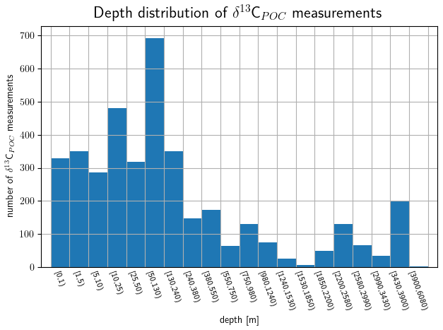
Figure 4 Vertical data coverage in depth layers based on the UVic grid: the uppermost 50 m is divided into subranges; below they are according to the UVic grid. The number of δ¹³C_POC data points available is plotted against its respective depth range.

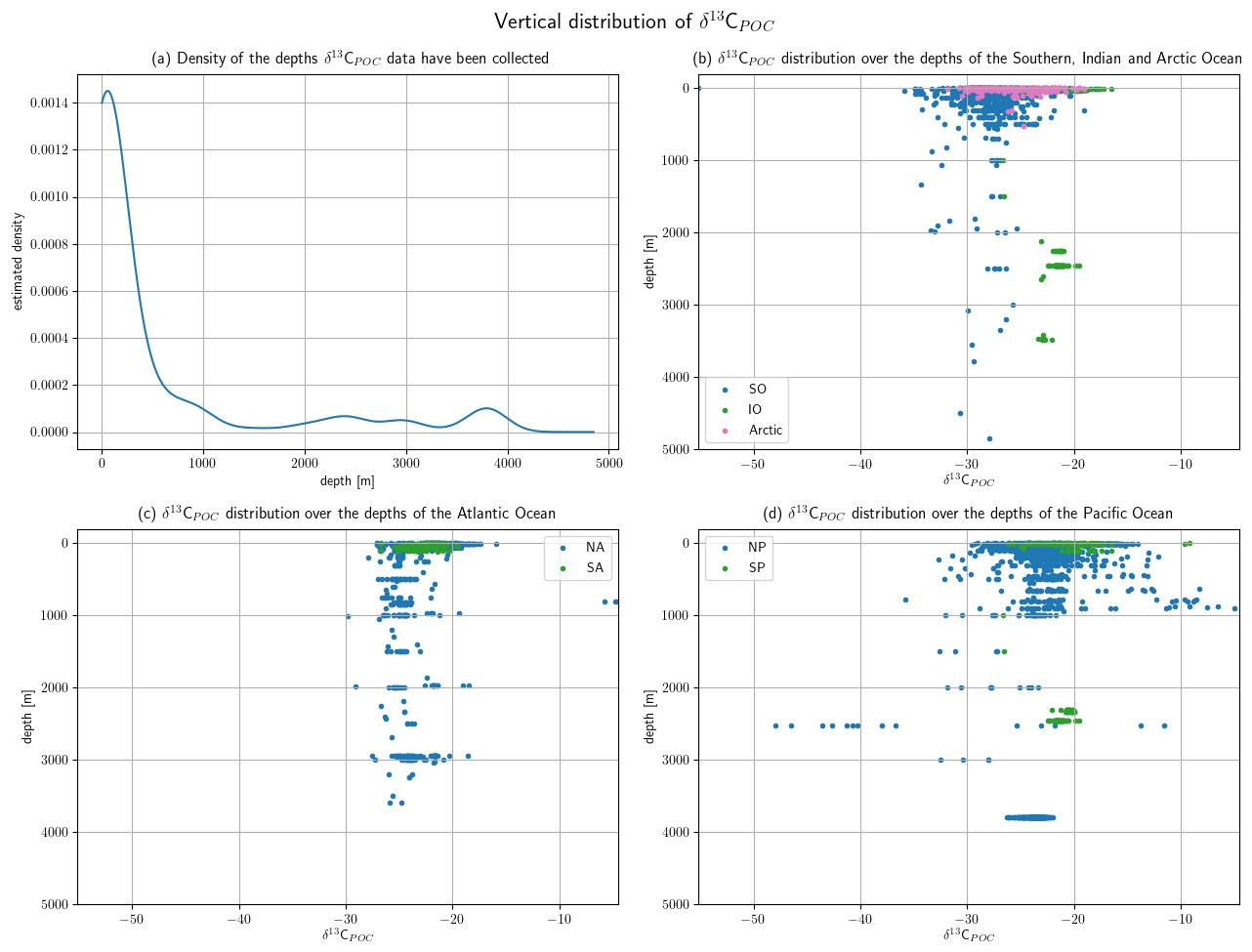
Figure 5 The vertical distribution of available δ¹³C_POC samples is shown (a) as the approximated density of the measurement depths and (b–d) as measured δ¹³C_POC values relative to their respective measurement depth. Panel (a) provides the estimated density of the depth values on the y axis and the depth in meters on the x axis. The estimation was realized by a Gaussian KDE. Panel (b) resolves the measurements of the Southern, Indian and Arctic Ocean, (c) the North Atlantic and South Atlantic, and (d) the North Pacific and South Pacific. The last three panels show the depth in meters on the y axis and the measured δ¹³C_POC value on the x axis. Different colors are used to mark different ocean basins.

Values of δ¹³C_POC are, apart from in the North Pacific, closely aligned within the individual ocean basins. The Atlantic, South Pacific and Indian Ocean show values mostly of −28 ‰ to −19 ‰. The δ¹³C_POC values in the Arctic reach down to approximately −30 ‰ and those in the Southern Ocean even to approximately −35 ‰. The North Pacific shows a wide spread of δ¹³C_POC values, especially between 50 and 100 m depth and at 2500 m depth. There they reach either down to less than −40 ‰ or up to more than approximately −10 ‰ at a depth of 2500 m.

Measurements in the North Atlantic, North Pacific and Indian Ocean reach down to more than 3500 m. Measurements down to nearly 5000 m were sampled in the Southern Ocean. The South Pacific was sampled down to a depth of 2500 m and the Arctic Ocean and South Atlantic only in the uppermost few hundred meters.

5.2 Horizontal distribution of the data set

All global oceans are covered with δ¹³C_POC data. In Fig. 6 the horizontal distribution of available data is depicted for both grids. For the UVic grid we show data from the file including all data independent of time; the WOA grid is averaged over all times. In both cases, we averaged data over all depths and also added data without depth information to best visualize the horizontal coverage. A similar plot, although with a different purpose, is given later in this work in Fig. 10 showing only surface data locations.

Figure 6 Global distribution of the δ¹³C_POC data is visualized based on the (a) UVic grid and (b) WOA grid. The data used for (a) are independent of time and include all available measurements with latitude and longitude information. The data shown in (b) include only data with complete temporal metadata and are averaged over the years 1964–2015. Both kinds of data are averaged over all measurements including data with missing depth information. Each colored square refers to a grid cell with available δ¹³C_POC measurements. The colors indicate the δ¹³C_POC value in the respective grid cell.

Many cruises are visible as lines formed by connected grid cells in Fig. 6, especially in the Atlantic and Indian Ocean and less so in the Southern Ocean. Also, smaller sample spots occur, mainly located in the Pacific, Arctic and Southern Ocean. The Atlantic Ocean provides the best data coverage. Then the Southern and Indian oceans contain the next best coverage with the North Pacific having the sparsest.

The highest δ¹³C_POC values are evident in low-latitude regions. In the Atlantic Ocean the highest values were measured between 0–30^∘ N and 30–60^∘ W as well as close to the western coast of France, reaching up to at least −17 ‰. The Indian Ocean shows generally high values of approximately −20 ‰. In the Pacific Ocean the highest values are close to the Peruvian coast and Papua New Guinea. We also find high values in the Bering Strait and on the northern edge of the Southern Ocean at around 65^∘ E.

The lowest δ¹³C_POC values are mostly found in the Southern Ocean. Nearly all measured grid cells here belong to δ¹³C_POC values lower than around −28 ‰. The Arctic Ocean shows low values as well, for instance in the Kara Sea. The lowest values in the Pacific Ocean occur in the Southern Ocean at high latitudes.

5.3 Meridional trend of δ¹³C_POC values

We show the north–south trend of δ¹³C_POC over the Atlantic Ocean based on the time-independent UVic grid and restricted to the uppermost 130 m, which resembles the euphotic zone in the UVic model. We chose this section due to it having the best data coverage. A biome mask according to Fay and McKinley (2014) was applied to the gridded data, thereby defining latitudinal zones in the entire Atlantic Ocean. Distributions of δ¹³C_POC within the biomes are shown in Fig. 7 (see also Table A3 in the Appendix).

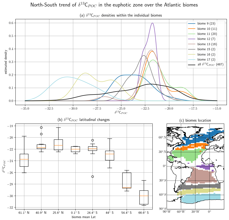
Figure 7 The north–south trend of sampled δ¹³C_POC values is visualized by a cross section over the Atlantic Ocean. Biomes (Fay and McKinley, 2014) define the latitudinal bands of the interpolated data set. Panel (a) presents a Gaussian KDE for each biome approximating the density of the contained δ¹³C_POC data. Different colors mark the individual biomes, and a black line shows the general global δ¹³C_POC distribution. The number in parentheses in each KDE label counts the number of δ¹³C_POC measurements used for the respective graph. Panel (b) shows in a box plot the steep decline in δ¹³C_POC values from the tropical biomes towards the higher latitudes. The x axis provides the mean latitudes of the biomes introduced in (a). The y axis measures the δ¹³C_POC value. Panel (c) shows the biome locations. Each biome is drawn in the color of its corresponding density estimate in (a) above. The biome numbers increase from the north to the south.

The biomes derived by Fay and McKinley (2014) are areas with consistent biological and ecological properties. The chosen biomes cover the Atlantic Ocean and extend to the Arctic Sea and parts of the Southern Ocean. The biomes are numbered 9 to 17, excluding 14. The biomes 15 to 17 represent parts of the Southern Ocean and were restricted to 70^∘ W and 20^∘ E. Their locations are shown in Fig. 7.

Observations by the biomes are consistent with the ones from Fig. 6. The two biomes showing the lowest δ¹³C_POC values from −28 ‰ to −29 ‰ are those located farthest south. The biome located farthest north contains the next-lowest values of about −24 ‰. The biomes with more positive δ¹³C_POC values are in the lower latitudes and show similarly higher values from −23 ‰ to −21 ‰.

6 Temporal distribution of the data set

The full δ¹³C_POC data cover a time period of around 50 years over 1964–2015 and all 12 calendar months. The number of samples measured during individual decades varies considerably with most measurements in the 1990s. Coverage within the months is quite comparable; only winter months in both hemispheres exhibit fewer data.

The distribution of δ¹³C_POC samples over the years is resolved in Table 4 and is visually approximated by Gaussian KDE in Fig. 8. The 1990s shows the best data coverage. More than half of the data points are associated with a year in this decade, which is visible by a pronounced maximum in the estimated density. The sparsest data are found in the 1960s, when only 74 data points were sampled. All other decades come with between around 300 and 600 δ¹³C_POC data points. The latest data are mostly from Anne Lorrain, MacKenzie et al. (2019) and Kaiser et al. (2019). The oldest data were taken from the data sets by Robyn Tuerena, Degens et al. (1968), and Eadie and Jeffrey (1973).

Table 4 Data coverage within the available decades: the first column lists the available decades and the second column the number of sampled δ¹³C_POC data points within this time frame.

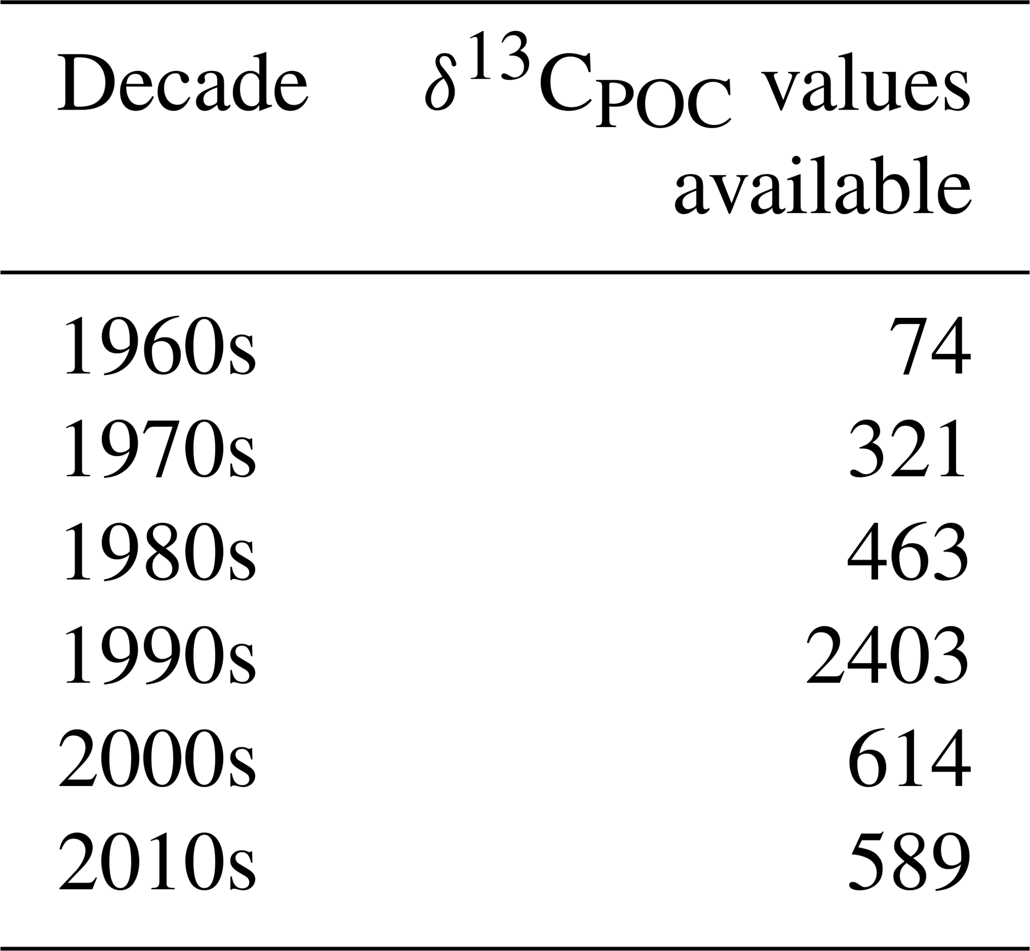
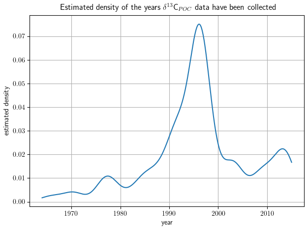
Figure 8 The distribution of δ¹³C_POC data samples over the years approximated by Gaussian KDE. The density is drawn on the y axis; the sample year is on the x axis. A higher altitude of the graph indicates years with more available data.

6.1 Monthly variations

Monthly clustered data of the Northern Hemisphere and Southern Hemisphere show monthly variations, but more observations are required to demonstrate robust seasonality within different regions. Since more than 50 % of the available δ¹³C_POC data originate in the 1990s, we selected data from this decade to exclude changes that might be introduced by longer-term trends. Furthermore, we restricted our data to the uppermost 130 m, which resembles the euphotic zone in the UVic model. In Fig. 9 we displayed all months with enough data points by a KDE and indicate the same months by the same colors. We excluded July, November and December in the Northern Hemisphere from this KDE representation because these months provided three or fewer data points each, which resulted in a KDE that overgrew the others by magnitudes and made their visual comparison difficult. The KDEs are supported by comparison of the median values of the individual months in Table 5.

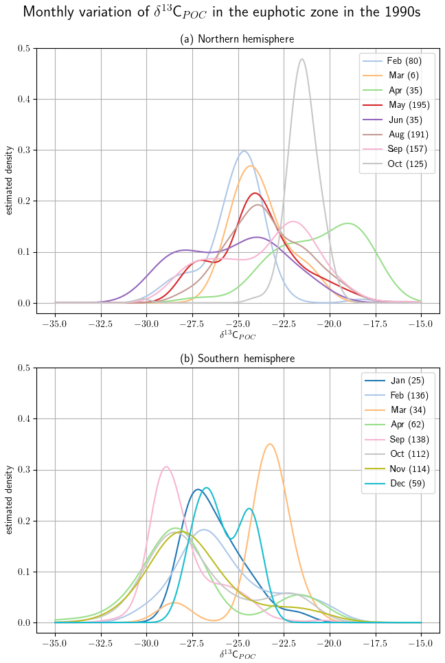
Figure 9 Monthly variations are split up by hemisphere with the Northern Hemisphere in (a) and Southern Hemisphere in (b). Due to their having the best data coverage, the analyses are carried out within the 1990s and in the uppermost 130 m. The δ¹³C_POC values are split up by sample month, and for every month with enough available data points (here more than three) a Gaussian KDE approximates their density. The number of used data points is given in each KDE label. For each hemisphere the densities are drawn all together; each month is indicated by an individual color.

Table 5 Monthly median change in δ¹³C_POC. Due to their having the best data coverage, the analyses were carried out within the 1990s and in the uppermost 130 m.

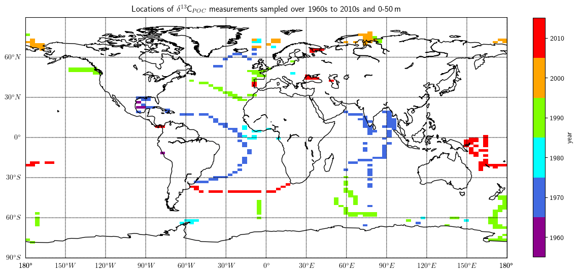
Figure 10 Grid locations of the δ¹³C_POC data, colored by sampling decades. Only data of the uppermost layer are considered in this plot. The different colors indicate the different sample decades and were plotted increasing in time above each other.

The monthly resolved variations in δ¹³C_POC do not reveal any significant seasonal pattern (Fig. 9; see also Table A4 in the Appendix). In general we find the highest δ¹³C_POC values in the Northern Hemisphere, with a median δ¹³C_POC of −20.4 ‰ in April and a median δ¹³C_POC of −21.5 ‰ in October, which are typical months with enhanced primary production (Northern Hemisphere spring and autumn blooms). Similarly high median δ¹³C_POC values cannot be ascertained for any month with data of the Southern Hemisphere, where values of δ¹³C_POC above −20 ‰ have rarely been observed at any time of the year. In fact, there is an overall tendency towards low δ¹³C_POC values for the Southern Hemisphere, which becomes well expressed during the months April and September, with medians of δ¹³C${}_{\mathrm{POC}}=-\mathrm{28.1}$ ‰ and δ¹³C${}_{\mathrm{POC}}=-\mathrm{28.5}$ ‰, respectively. However, interpretations of this north–south trend should be treated with caution because the apparent tendency is likely conditioned by some imbalance in the number of high-latitude data points. Compared to the number of data points from the Southern Ocean, samples from the Arctic Ocean are considerably underrepresented (see also Fig. 10). Furthermore, the discrimination between data of the Northern Hemisphere and Southern Hemisphere is crude, and we encourage the use of our data collection for more advanced analyses of seasonal, monthly based changes in the δ¹³C_POC signal.

6.2 Decadal variations

The decadal UVic grid NetCDF files are the basis for showing long-term changes in the δ¹³C_POC data. An overview of where the data within the individual decades were sampled is given in Fig. 10. This shows that the sparsest coverage was obtained in the 1960s, located close to the central American continent. Most data in the Indian Ocean were sampled in the 1970s. A cruise across the southern part of the Atlantic Ocean up to 30^∘ N and some samples close to Iceland were also measured in this decade. The 1980s is similarly sparse in spatial coverage to the 1960s. Measurements of the 1980s were taken at locations in the Southern Ocean, in the Arctic and in the Atlantic close to the Equator. The 1990s has the best coverage including most ocean basins. Most Southern Ocean data were sampled within the 1990s. The 2000s provides good coverage of the Arctic Ocean. Finally, the 2010s data were mostly sampled in the Southern Hemisphere in the open Pacific and Atlantic. A smaller number of Eurasian continental sea data were also part of the 2010s samples.

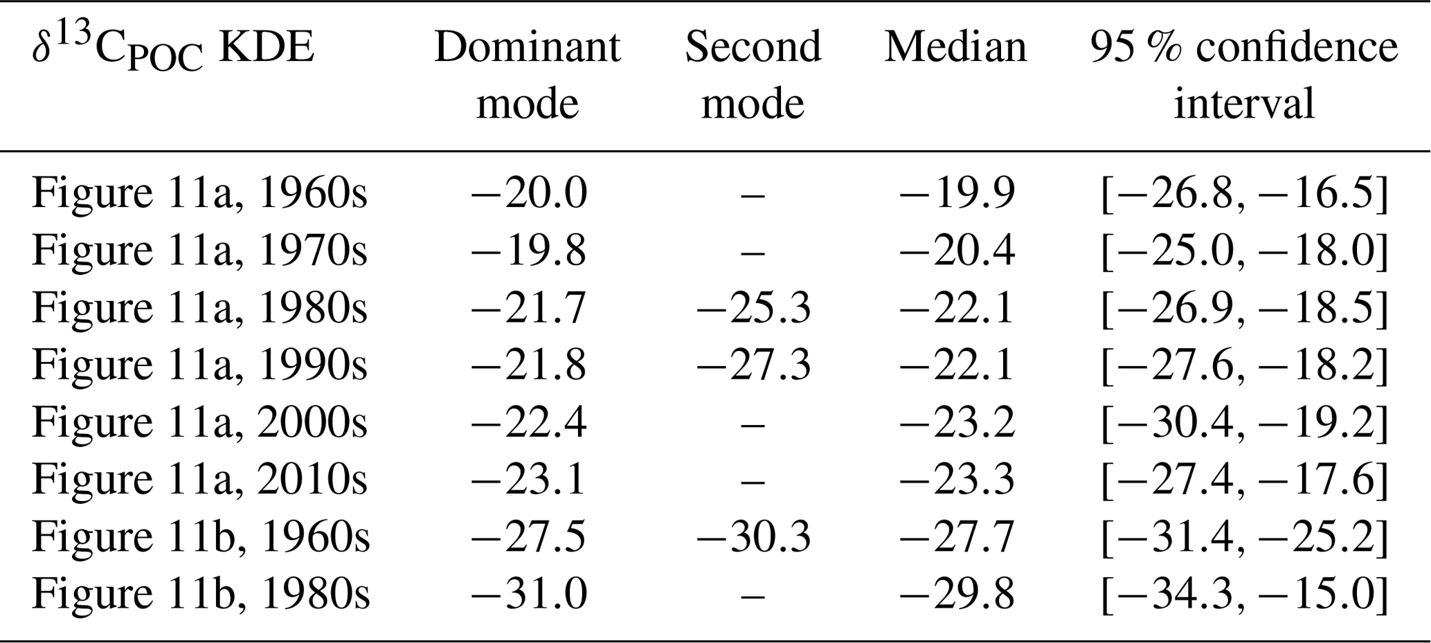
We show the changes in δ¹³C_POC values over the available decades by density estimates in Fig. 11 (see also Table A5 in the Appendix) and by their median in Fig. 12. Figure 11 visualizes the sparse coverage of the Southern Ocean outside of the 1990s, which is why the area is not part of any further discussion here. The Southern Ocean is defined as the ocean area south of 45^∘ S. All presented analyses were restricted to the euphotic zone, i.e., the uppermost 130 m resembling the two first layers of the UVic grid.

Figure 11 The decadal shift in δ¹³C_POC values for all but the Southern Ocean (a) and only the Southern Ocean (b) shown by estimated densities of δ¹³C_POC values. The differently colored graphs refer to the individual decades. Southern Ocean data are sparsely covered, and the region does not provide enough data for a reasonable comparison.

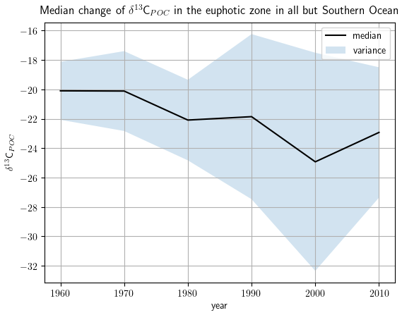
Figure 12 The decadal shift in δ¹³C_POC values in the uppermost 130 m for all but the Southern Ocean: δ¹³C_POC decadal median against the decades. The shaded area around the graph marks the variance of the respective decade in each direction.

A clear decrease in δ¹³C_POC densities in Fig. 11 can be identified for the global ocean outside of the Southern Ocean. All decades but the 1980s show one clear maximum in their approximated densities. The 1980s shows a second expressed density maximum at lower values. The main maximum shifts from the 1960s at δ¹³C${}_{\mathrm{POC}}\approx -\mathrm{19.9}$ ‰ to the 2010s at δ¹³C${}_{\mathrm{POC}}\approx -\mathrm{23}$ ‰. This decrease is also clearly visible in the comparison of the decadal medians (Fig. 12). The Southern Ocean provides far worse data coverage. Only the 1980s and 1990s include enough data to construct a comparable KDE. Due to this very low data availability, all of these results must be taken with the highest caution.

7 Data availability

The described δ¹³C_POC data are available at https://doi.org/10.1594/PANGAEA.929931 (Verwega et al., 2021).

8 Conclusions

The aim of this work was to construct the largest publicly accessible δ¹³C_POC data set. The starting point of our collection and analyses was the readily available data collection of Goericke (1994), which comprised 467 data points. Our primary objective was to elaborate this set of data by adding useful meta-information from the original publications and by introducing additional δ¹³C_POC measurements, as recorded in the world ocean database PANGAEA and made available by Robyn Tuerena and Anne Lorrain. This way we could expand the data collection substantially, from the original 467 to 4732 data points. This new δ¹³C_POC data set provides the best coverage to date and will be a useful tool to help constrain many marine carbon cycling processes and pathways from ocean–atmosphere exchange to marine ecosystems, as well as to better understand observations and validate models. To ensure dynamic growth of our data collection, the corresponding author will provide annual updates of the data set. Furthermore, he may be contacted by any interested researcher who would like to add their data to this collection.

The data are provided in a csv structure and interpolated onto two different global grids in NetCDF format. The csv file contains the δ¹³C_POC values, their anomalies to their mean and all available meta-information. The interpolations are provided on a coarse $\mathrm{1.8}{}^{\circ }\times \mathrm{3.6}{}^{\circ }$ grid of a δ¹³C_POC-simulating model and a finer $\mathrm{1}{}^{\circ }\times \mathrm{1}{}^{\circ }$ grid by the World Ocean Atlas. We have provided a detailed description of our data collection procedure, all added meta-information and data coverage as well of the interpolation procedure carried out. We took the utmost care to make all data coherent, comparable and back-trackable and all adjustments transparent. Assumptions, changes and deletions of the used data sets have been described in detail.

We have described the general spatial and temporal trends of the sampled δ¹³C_POC data of the raw data file. Distributions were always approximated by Gaussian kernel density estimators. The data range from 1964–2015 with by far the best coverage in the 1990s. Sample locations reach down to a depth of nearly 5000 m and best cover the uppermost 10 m, especially in the Atlantic and Indian Ocean. We were able to show our δ¹³C_POC data values are mostly located between δ¹³C${}_{\mathrm{POC}}=-\mathrm{15}$ ‰ and δ¹³C${}_{\mathrm{POC}}=-\mathrm{35}$ ‰ with two maxima at around δ¹³C${}_{\mathrm{POC}}=-\mathrm{27}$ ‰ and δ¹³C${}_{\mathrm{POC}}=-\mathrm{23}$ ‰, the latter one being more pronounced. A comparison of the main sample methods showed consistent results when compared with regions. δ¹³C_POC data separated by months indicate counteracting seasonal trends in both hemispheres, but more data are required to demonstrate robust seasonality.

The interpolated data provide insights into geographical behavior of the sampled δ¹³C_POC data. We showed a good general coverage of all global oceans by δ¹³C_POC but observed a lack of data in PANGAEA that cover North Pacific regions. Since the Atlantic Ocean provides the best coverage, corresponding data were used for a north–south trend analysis, where we observed that the lowest values (⪅−28 ‰) can be found in the Southern Ocean, whereas the highest (⪆−22 ‰) are restricted to low-latitude regions. This might also have influenced the observed lower δ¹³C_POC values in the Southern Hemisphere compared to the Northern Hemisphere, due to the relatively good coverage of the Southern Ocean. Finally, we showed the sample locations and value development of δ¹³C_POC over the observed decades. Since the Southern Ocean data were mainly sampled in the 1990s, a significant multi-decadal trend could not be detected there. In all other oceans our δ¹³C_POC data show a decrease by about 3 ‰ over the observed time frame, which is about double the rate of the known Suess effect (Keeling, 1979) on aqueous δ¹³CO₂ (Young et al., 2013). This corroborates an increase in phytoplankton carbon fractionation that may be associated with a change in phytoplankton communities as previously suggested (Lorrain et al., 2020; Young et al., 2013). The data set shows promise for better understanding, constraining and prediction of carbon cycling as it provides a validation tool for mechanistic models and supports separation of non-spatial components in δ¹³C_POC variations.

Appendix A: Statistical properties of δ¹³C_POC kernel density estimates

In Tables A1, A2, A3, A4 and A5 we present the modes, medians and confidence limits of the KDEs derived in Figs. 1, 3, 7, 9 and 11, respectively.

Table A1 Statistical properties of the KDE derived for Fig. 1 evaluated on an equidistant grid over $[-\mathrm{55.15},-\mathrm{4.5}]$ with 1001 grid points: the first column indicates the respective KDE, the following two its modes, the fourth the median and the fifth the 95 % confidence interval of the respective KDE. All values are given in per mill.

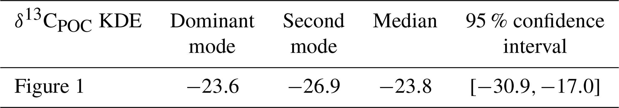
Table A2 Statistical properties of the KDEs derived for Fig. 3 evaluated on an equidistant grid over $[-\mathrm{35},-\mathrm{15}]$ with 1001 grid points: the first column indicates the respective KDE, the following two its modes, the fourth the median and the fifth the 95 % confidence interval of the respective KDE. All values are given in per mill.

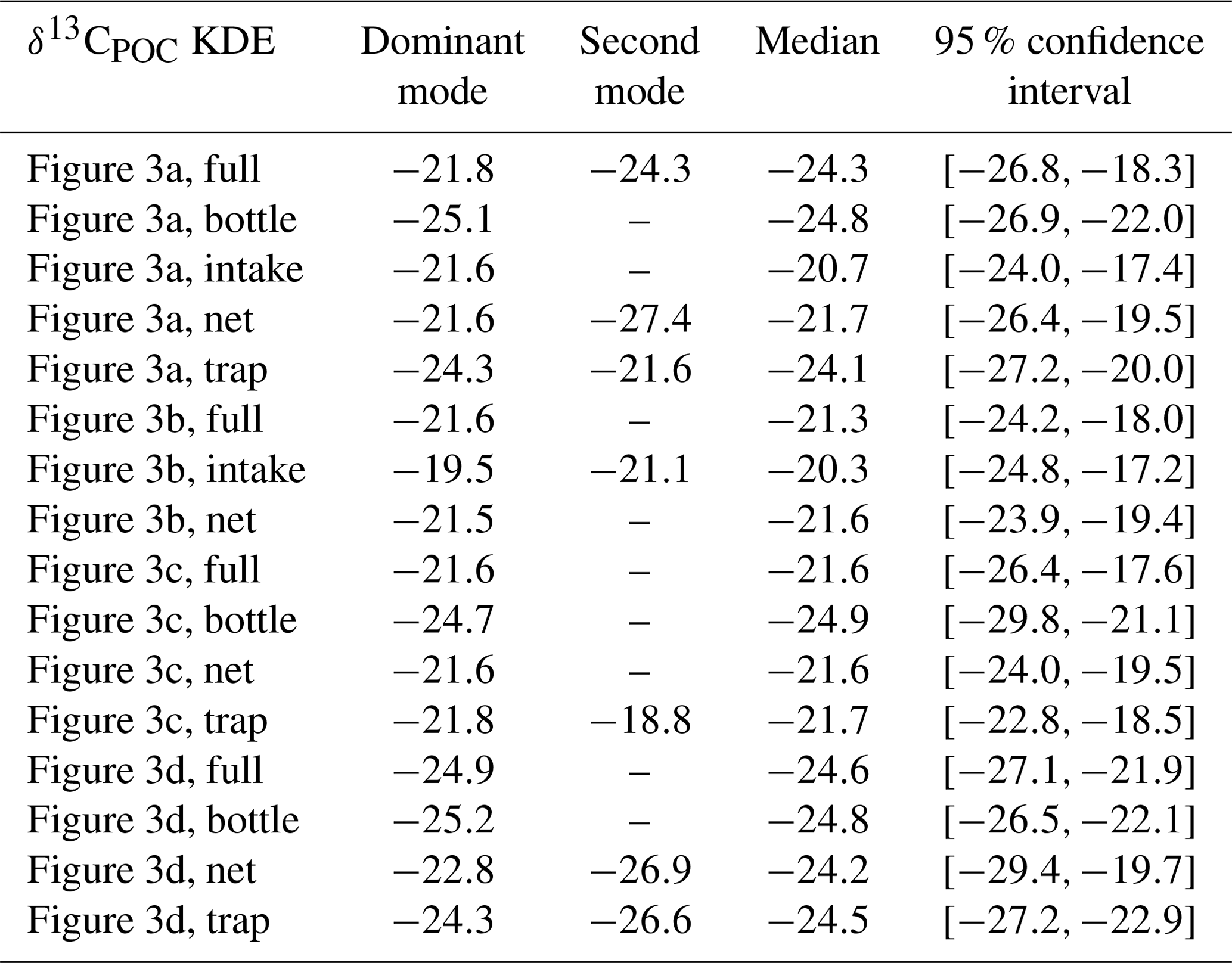
Table A3 Statistical properties of the KDEs derived for Fig. 7 evaluated on an equidistant grid over $[-\mathrm{35},-\mathrm{15}]$ with 1001 grid points: the first column indicates the respective KDE, the following two its modes, the fourth the median and the fifth the 95 % confidence interval of the respective KDE. All values are given in per mill.

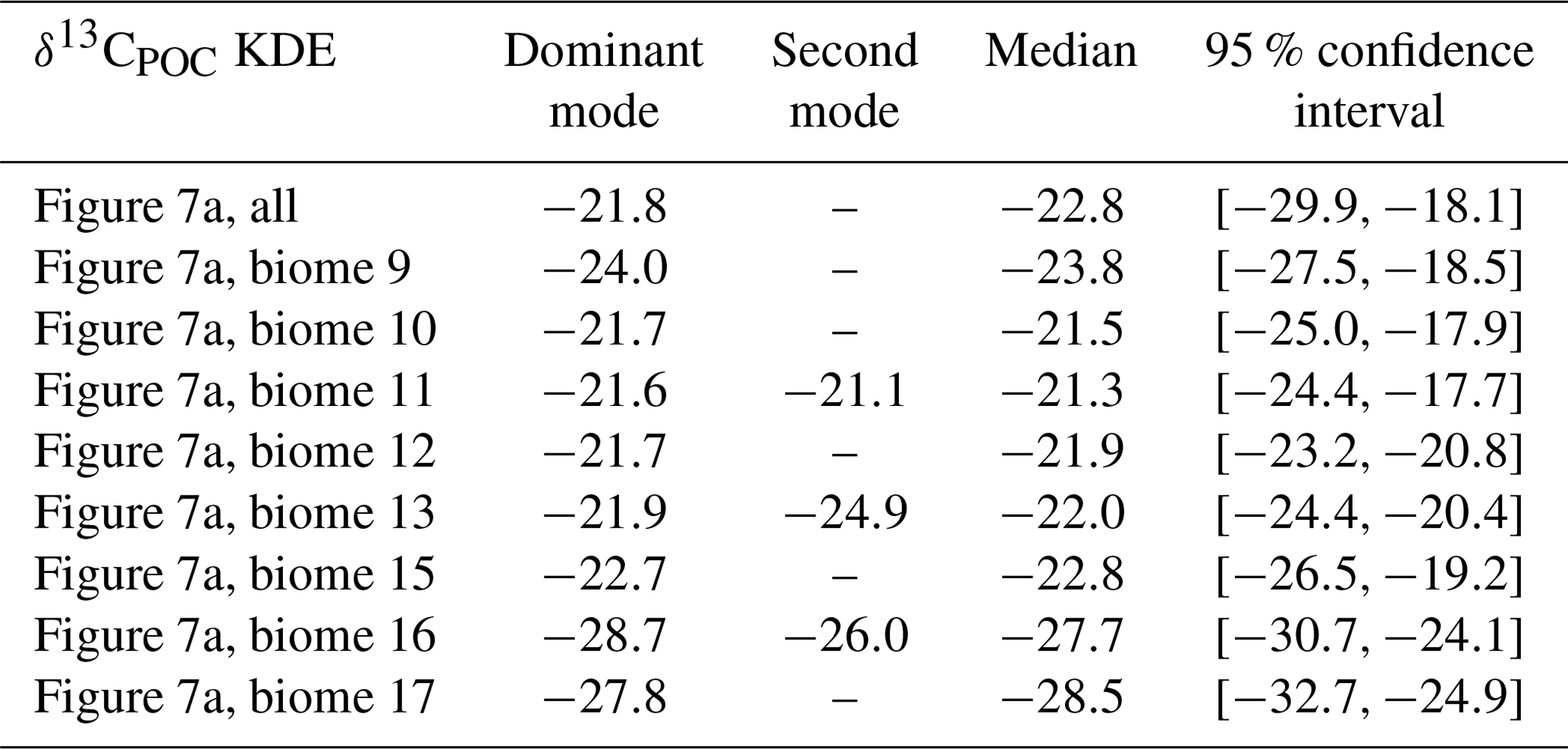
Table A4 Statistical properties of the KDEs derived for Fig. 9 evaluated on an equidistant grid over $[-\mathrm{35},-\mathrm{15}]$ with 1001 grid points: the first column indicates the respective KDE, the following two its modes, the fourth the median and the fifth the 95 % confidence interval of the respective KDE. All values are given in per mill.

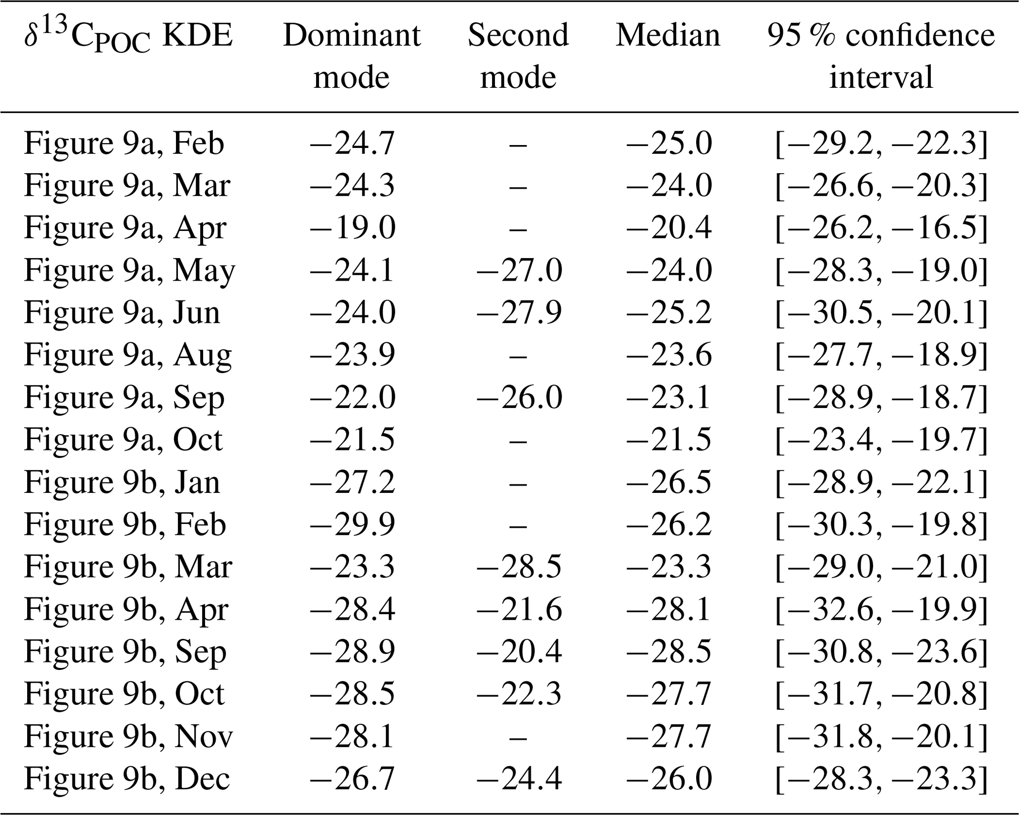
Table A5 Statistical properties of the KDEs derived for Fig. 11 evaluated on an equidistant grid over $[-\mathrm{35},-\mathrm{15}]$ with 1001 grid points: the first column indicates the respective KDE, the following two its modes, the fourth the median and the fifth the 95 % confidence interval of the respective KDE. All values are given in per mill.