the Creative Commons Attribution 4.0 License.
the Creative Commons Attribution 4.0 License.
 | 15 Oct 2021
A first investigation of hydrogeology and hydrogeophysics of the Maqu catchment in the Yellow River source region
Mengna Li
Maciek W. Lubczynski
Jean Roy
Lianyu Yu
Hui Qian
Zhenyu Li
Jie Chen
Lei Han
Han Zheng
Tom Veldkamp
Jeroen M. Schoorl
Harrie-Jan Hendricks Franssen
Kai Hou
Qiying Zhang
Panpan Xu
Fan Li
Kai Lu
Yulin Li
Zhongbo Su
The Tibetan Plateau is the source of most of Asia's major rivers and has been called the Asian Water Tower. Detailed knowledge of its hydrogeology is paramount to enable the understanding of groundwater dynamics, which plays a vital role in headwater areas like the Tibetan Plateau. Nevertheless, due to its remoteness and the harsh environment, there is a lack of field survey data to investigate its hydrogeology. In this study, borehole core lithology analysis, soil thickness measurement, an altitude survey, hydrogeological surveys, and hydrogeophysical surveys (e.g. magnetic resonance sounding – MRS, electrical resistivity tomography – ERT, and transient electromagnetic – TEM) were conducted in the Maqu catchment within the Yellow River source region (YRSR). The hydrogeological surveys reveal that groundwater flows from the west to the east, recharging the Yellow River. The hydraulic conductivity ranges from 0.2 to 12.4 m d−1. The MRS sounding results, i.e. water content and hydraulic conductivity, confirmed the presence of an unconfined aquifer in the flat eastern area. Based on TEM results, the depth of the Yellow River deposits was derived at several places in the flat eastern area, ranging from 50 to 208 m. The soil thickness measurements were done in the western mountainous area of the catchment, where hydrogeophysical and hydrogeological surveys were difficult to be carried out. The results indicate that most soil thicknesses, except on the valley floor, are within 1.2 m in the western mountainous area of the catchment, and the soil thickness decreases as the slope increases. These survey data and results can contribute to integrated hydrological modelling and water cycle analysis to improve a full-picture understanding of the water cycle at the Maqu catchment in the YRSR. The raw dataset is freely available at https://doi.org/10.17026/dans-z6t-zpn7 (Li et al., 2020a), and the dataset containing the processed ERT, MRS, and TEM data is also available at the National Tibetan Plateau Data Center with the link https://doi.org/10.11888/Hydro.tpdc.271221 (Li et al., 2020b).
- Article
(14165 KB) - Full-text XML
-
Supplement
(3106 KB) - BibTeX
- EndNote


With a huge amount of water storage, the Tibetan Plateau (TP) acts as the “Water Tower of Asia” (Qu et al., 2019; Wang et al., 2017), recharging many major Asian rivers including the Salween, Mekong, Brahmaputra, Irrawaddy, Indus, Ganges, Yellow, and Yangtze rivers (Immerzeel et al., 2009), feeding more than 1.4 billion people (Immerzeel et al., 2010) and promoting regional social and economic development (Xiang et al., 2016). Due to climate change, the TP has experienced accelerated temperature rise over the past decades (Huang et al., 2017). Since the 1950s, the warming rate over the TP ranges between 0.16–0.36 ∘C per decade and rises to 0.50–0.67 ∘C per decade from the 1980s (Kuang and Jiao, 2016). The retreating glaciers and snow cover, decreasing wetland area, and rising snow lines indicate that the hydrological system on the TP is undergoing profound changes (Kang et al., 2010; Li et al., 2019; Xu et al., 2016; Yao et al., 2013).
So far, the groundwater-related studies on the TP are mainly satellite-based, focusing on using the Gravity Recovery and Climate Experiment (GRACE) to estimate terrestrial water storage, which consists of surface and subsurface water (Haile, 2011; Jiao et al., 2015; Zhong et al., 2009). Among those studies, Xiang et al. (2016) separated the groundwater storage from terrestrial water storage observed by GRACE using four land surface models: the Community Land Model (CLM), Mosaic, Noah, and the Variable Infiltration Capacity (VIC) model of the Global Land Data Assimilation System (GLDAS) (Rodell et al., 2004), Climate Prediction Center (CPC) soil moisture data (Fan and Van Den Dool, 2004), and a glacial isostatic adjustment model.
An integrated surface-groundwater model is essential for improving understanding of different processes quantitatively (Graham and Butts, 2005). To set up an integrated surface-groundwater model, different kinds of data are needed for the parameterization of land surface and subsurface but also for atmospheric forcing and state variables that are required for model calibration and validation. Land surface data such as topography, land cover, and soil parameters can be obtained from digital elevation models (DEMs) and regional or global soil databases (Su et al., 2011; Zhao et al., 2018). Atmospheric forcing data, including precipitation, air temperature, wind velocity, and other variables, are available from regional or global meteorological datasets (Li et al., 2017; Su et al., 2013, 2020; Yang, 2017).
Subsurface data, like hydrogeological information (e.g. lithology, water table depth, hydrogeological parameters) and state variables (e.g. hydraulic heads and soil moisture content at root zone or of deeper layers), usually require in situ measurements. These hydrogeology-related data are the most difficult ones to acquire. Efforts have been made to develop the global map of permeability (Gleeson et al., 2014, 2011), hydraulic conductivity (Gupta et al., 2021; Montzka et al., 2017), groundwater table depth (Fan et al., 2013), and groundwater volume and distribution (Gleeson et al., 2016). However, global subsurface databases suffer large uncertainty, mainly because of spatial heterogeneity and scale effects that can be resolved only by field measurements. The TP lacks such measurements due to its remoteness and harsh environment (Yao et al., 2019). Lately, the Chinese Academy of Science (CAS) launched the CAS Earth Poles project (X. Li et al., 2020, 2021), which aims to address the bottleneck of polar (high-mountain cold region) data curation, integration, and sharing, which is expected to overcome some of the aforementioned difficulties.
The conventional way to acquire hydrogeological information in an unknown area is by augering or drilling boreholes and carrying out hydraulic tests, for example, pumping tests (Vouillamoz et al., 2012). However, due to the harsh environment of the TP and the high costs and time-consuming nature of the traditional hydrogeological survey methods, little hydrogeological work has been done on the TP.
The hydrogeophysical methods are up and coming in hydrogeological studies (Chirindja et al., 2016). They have been applied in various conditions, for example in wetlands (Chambers et al., 2014), rivers (Steelman et al., 2015), proglacial moraines (McClymont et al., 2011), karst regions (McCormack et al., 2017), and volcanic systems (Di Napoli et al., 2016; Fikos et al., 2012). Compared to other hydrogeophysical methods, such as seismic, gravity, and resistivity methods, magnetic resonance sounding (MRS) is the only method that is able to detect the free water in the subsurface directly (Lubczynski and Roy, 2003, 2004) and quantify hydrogeological parameters and water storage (Lachassagne et al., 2005; Legchenko et al., 2002, 2018; Lubczynski and Roy, 2007).
The MRS method is based on the nuclear magnetic resonance (NMR) principle, widely implemented in medical magnetic resonance imaging (MRI). In contrast to MRI, the MRS excitation is done at the Larmor frequency corresponding to the local magnetic field of the Earth, which propagates and gets attenuated through conductive subsurface media. Therefore, at a given position of the Earth, MRS signal response depends on the strength of the Earth's magnetic field, and on the strength of the natural and artificial noise (Lubczynski and Roy, 2004) but also on the subsurface resistivity. The electrical resistivity measurement is suggested to be jointly used with MRS (Braun and Yaramanci, 2008; Descloitres et al., 2007; Vouillamoz et al., 2002). Electrical resistivity tomography (ERT) is one of the predominantly employed hydrogeophysical methods to estimate the subsurface electrical resistivity (Herckenrath et al., 2012; Jiang et al., 2018). It has been widely applied together with MRS to explore regional hydrogeology (Vouillamoz et al., 2003; Descloitres et al., 2008; Pérez-Bielsa et al., 2012). Furthermore, the transient electromagnetic survey (TEM), referred to as the time domain electromagnetic (TDEM) method, also provides subsurface resistivity but is able to achieve deeper penetration than ERT. The ERT has already been used on the TP by Gao et al. (2019) and You et al. (2013) to investigate permafrost. Nevertheless, we have not seen the combined use of MRS, ERT, and TEM for hydrogeophysical surveys over the TP.
Investigations on various fields, such as geomorphology, climate change, glacier, and permafrost, have been done on the TP based on different DEMs. Zhang et al. (2006) analysed the geomorphic characteristics of the Minjiang drainage basin with SRTM (Shuttle Radar Topography Mission) data. Wei and Fang (2013) assessed the trends of climate change and the spatiotemporal differences over the TP from 1961–2010, with a generalized temperature zone–elevation model and SRTM. Ye et al. (2015) calculated the glacier elevation change in the Rongbuk catchment from 1974 to 2006 based on topographic maps and ALOS (Advanced Land Observing Satellite). Niu et al. (2018) mapped permafrost distribution throughout the Qinghai–Tibet Engineering Corridor based on ASTER (the Terra Advanced Spaceborne Thermal Emission and Reflection Radiometer) global DEM. However, different DEMs used in different studies may lead to potential inconsistencies for understanding relevant physical processes (Zeng et al., 2019, 2015). For the Maqu catchment, located within the TP and being the focus of this study, it is crucial to evaluate the accuracy of different DEMs to select the best one and eventually calibrate it using ground measurements since altitude is used to calculate hydraulic heads, which determine and control groundwater flow. Therefore, it is important to evaluate the accuracy of satellite DEM products with a ground-based real-time kinematic global positioning system (GPS-RTK); such works have not been common over the TP.
This study jointly uses hydrogeological and hydrogeophysical methods, including aquifer tests, MRS, ERT, TEM, and other necessary approaches at the Maqu catchment in the Yellow River source region (YRSR) on the TP. The paper focuses on field hydrogeological and hydrogeophysical surveys and corresponding datasets, aiming to fill the scientific data gap on the TP. In what follows, the study area is introduced in Sect. 2. Borehole core lithology analysis, soil thickness measurement, altitude surveys, hydrogeological surveys, and hydrogeophysical surveys are presented in Sect. 3. The results are documented and uncertainties are discussed in Sect. 4. Data availability is given in Sect. 5. Conclusions are made in Sect. 6.
The study area is a catchment (33∘43′–33∘58′ N, 101∘51′–102∘16′ E) in Maqu County, China (Fig. 1). It is located at the north-eastern edge of the TP, the first major bend of the Yellow River. Maqu County is regarded as the “reservoir” of the YRSR. The part of the Yellow River in contact with the Maqu catchment is about 36 km long, while the whole length passing Maqu County is 433.3 km. When the Yellow River flows through Maqu County, the annual run-off increases by 10.8×10⁹ m3, accounting for 58.7 % of the total run-off of 18.4×10⁹ m3 of the Yellow River in the YRSR (Wang, 2008). The Maqu catchment is characterized by a cold climate with dry winter and warm summer, assigned as Dwb in the updated Köppen–Geiger climate classification (Peel et al., 2007). The annual mean temperature is about 1.8 ∘C, and the precipitation is around 620 mm annually. The catchment is covered by short grasses used for grazing by yaks and sheep. The elevation ranges between 3367 and 4017 m a.s.l. according to ALOS PALSAR (Phase Array type L-band Synthetic Aperture Radar) RT1 (high terrain correction resolution). There is a reservoir in the catchment (Fig. 1c) with functions of grassland irrigation and flood control.
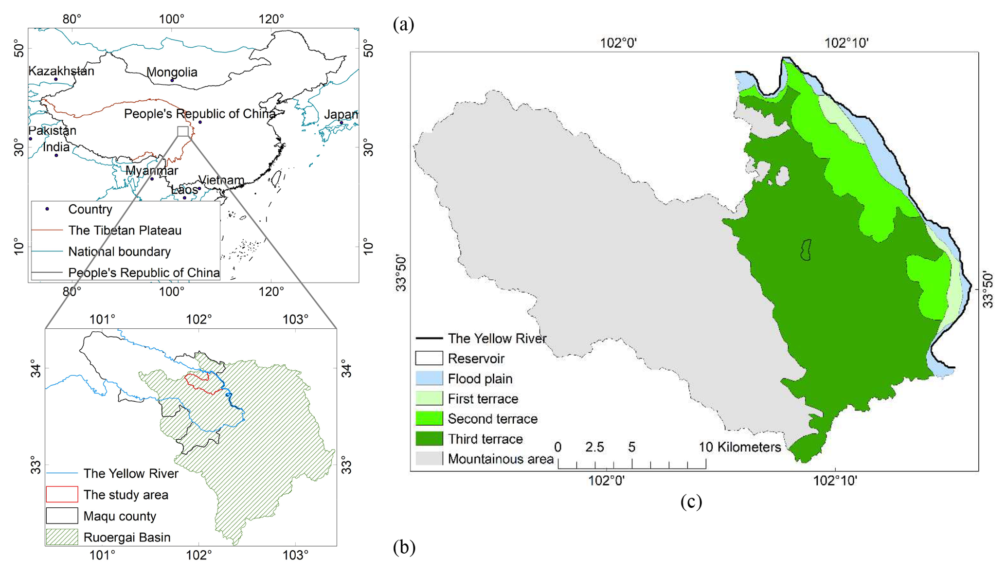
Figure 1The geographical location of Maqu catchment, Maqu County, and Ruoergai basin on the TP and geomorphologic map: (a) the geographical location and boundary of the TP (Zhang et al., 2014a, b); (b) the geographical location of the Maqu catchment, Maqu County, and Ruoergai basin (Li and Gao, 2019); (c) the geomorphologic map of Maqu catchment.
Based on the field survey of geomorphology and geology (Compton, 1962; Dackombe and Gardiner, 2020), the catchment can be divided into two parts, the flat eastern area and the western mountainous area. The western mountains are feldspathic quartzose sandstone and sandy slate with soil covered at the top, while the eastern, relatively flat part is composed mainly of sediments, such as alluvial deposits with intercalated aeolian units. The eastern part, together with its extension outside of the study area, is called the Ruoergai basin (Fig. 1b). Surface processes cause erosion, mixing, unmixing, and redistribution of alluvial materials within the thick alluvia accumulation in the eastern part. Geomorphological characterization was carried out in the Maqu catchment in 2018, and the three terraces were identified (Fig. 1c).
Some previous works have been done in or around the catchment. Su et al. (2011) monitored the soil moisture and soil temperature from 5 to 80 cm below the ground surface. Dente et al. (2012) assessed the reliability of AMSR-E (Advanced Microwave Scanning Radiometer for Earth Observing System) and ASCAT (Advanced Scatterometer) soil moisture products. Zheng et al. (2016) investigated the impacts of Noah model physics on catchment-scale run-off simulations. Zeng et al. (2016) combined the in situ soil moisture networks with the classification of climate zones to produce the in-situ-measured soil moisture climatology at the plateau scale. Zhao et al. (2018) studied the soil hydraulic and thermal properties of the 0.8 m top soil column. Zhuang et al. (2020) blended the surface soil moisture data from satellites, land data assimilation, and in situ measurements with the constraint of in situ data climatology and estimated the root zone soil moisture by scaling the blended surface soil moisture product. The present research focuses on the hydrogeological and hydrogeophysical aspects, complementing previous studies.
Figure 2 shows the fieldwork workflow towards establishing a hydrogeological conceptual model, which is beyond the scope of this study and will be presented in a future study. The workflow includes the borehole core lithology analysis, soil thickness measurement, an altitude survey, hydrogeological surveys, and hydrogeophysical surveys (Table 1 and Fig. 2). Yellow boxes in Fig. 2 represent the fieldwork, and green boxes represent the results of fieldwork, which will finally contribute to the set-up of the hydrogeological conceptual model. The obtained information on lithology, soil thickness, and ground surface elevation provides basic knowledge in the study area. Hydrogeological measurements of water table depth and hydraulic conductivity provide important input that can be used to deduce the direction and rate of regional groundwater flow, which is beyond the scope of this study. For hydrogeophysical results, magnetic susceptibility measurements ensure the suitability of applying MRS, while underground resistivity measurements from ERT are used in the inversion of MRS for deriving water content and transmissivity. TEM provides deeper resistivity information than other methods and estimates the depth of the hydrogeological boundary. The locations of the surveys and measurements are shown in Figs. 3, 4, and 5.
Table 1Methods, equipment, and timing for carrying out relevant measurements as in Fig. 2.
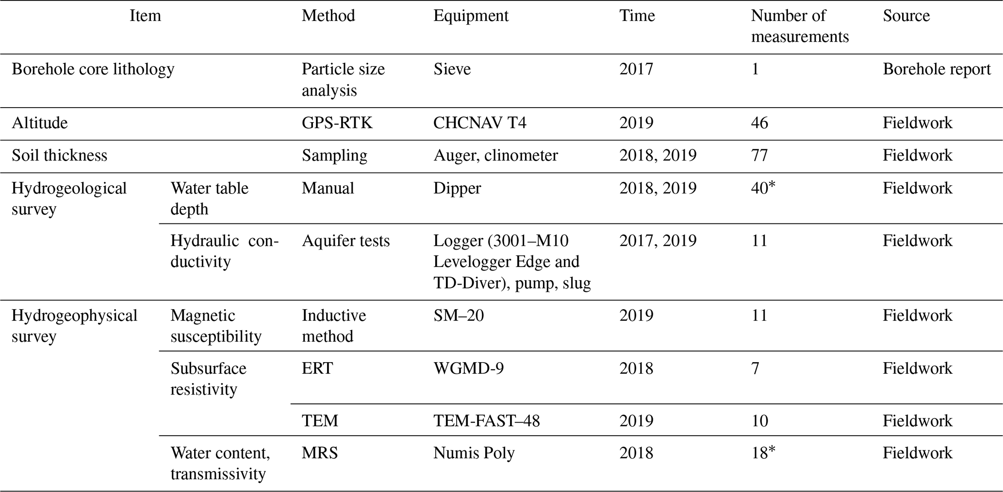
*40 water table depths were measured instantaneously in 34 boreholes in 2018 and 2019.
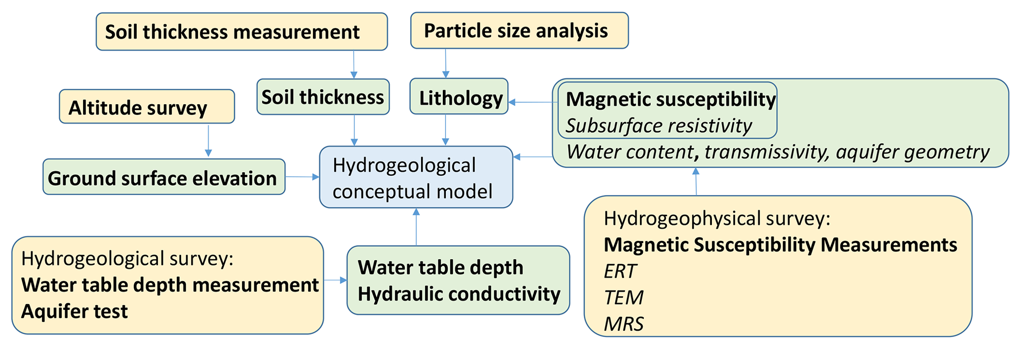
Figure 2Fieldwork workflow for setting up a hydrogeological conceptual model at Maqu catchment, where italics represent indirect technique (e.g. inversion type of retrieval) with unknown uncertainty, regular bold letters represent direct technique with low uncertainty, and regular letters do not convey uncertainty information.
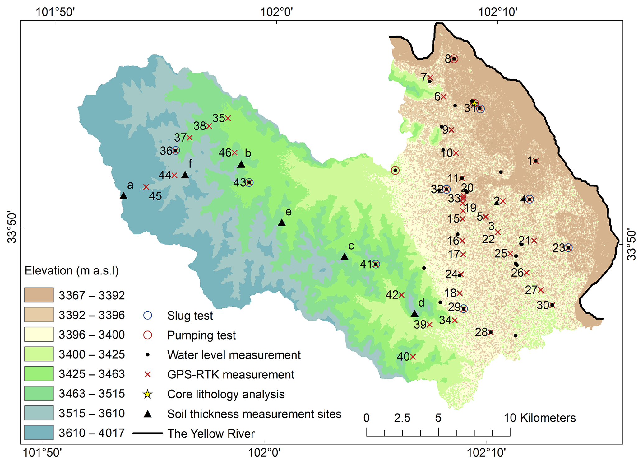
Figure 3Locations of the hydrogeological surveys, ground surface elevation measurements, core lithology analysis, and soil thickness measurements. The numbers from 1 to 46 (due to limited space, several numbers are not shown in the figure) indicate the measurement sequence of GPS-RTK.

Figure 4Panels (a), (b), (c), (d), (e), and (f) are the exact locations of soil thickness measurements at the sites a, b, c, d, e, and f, respectively, shown in Fig. 3, in the .KML-formatted image from © Google Earth.
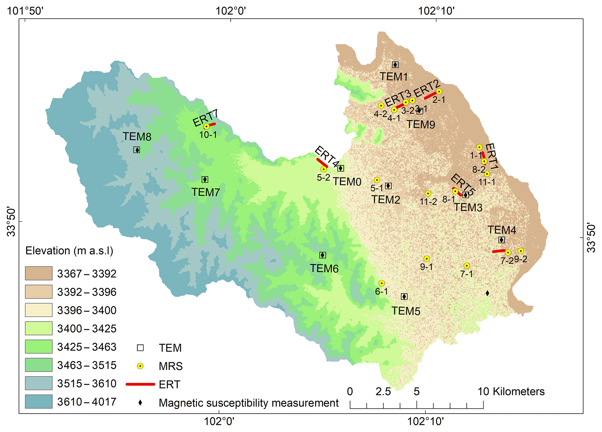
Figure 5Location of hydrogeophysical surveys.
3.1 Borehole core lithology
The borehole core lithology is helpful in terms of understanding the formation of an area, assessing geometry of aquifers, and estimating hydrogeological parameters. Some boreholes were available for water table depth measurement in the study area, but information of borehole core lithology was only available in one borehole (ITC_Maqu_1; shown in Fig. 3 as core lithology analysis) drilled in 2017 down to the depth of 32 m from the ground surface. The lithology of the cores was determined based on particle size analysis using the sieving method with mesh sizes of 60, 40, 20, 10, 5, 2, 1, 0.5, 0.25, and 0.075 mm.
3.2 Soil thickness measurement
In the mountainous west, where transportation and set-up of hydrogeophysical surveys are difficult, we auger-sampled the thickness of the overlying soils (Fig. 3) to build the hydrogeological conceptual model and to validate simulations of spatially distributed soil thickness by the landscape evolution model LAPSUS (LandscApe ProcesS modeling at mUlti-dimensions and scaleS) (Schoorl et al., 2006, 2002) (relevant details will be presented in another study). The fieldwork was carried out at six sites (Fig. 4a–f). Measurements at sites 1 and 2 were conducted in 2018, while the rest were conducted in 2019. Soil thickness and slope of the ground surface were measured using an auger and a clinometer from Eijkelkamp Soil & Water Company (https://en.eijkelkamp.com, last access: 4 March 2021). The exact measurement positions at each site (Fig. 4) were decided based on slope forms and surface pathways.
3.3 Altitude survey
The accuracy of ground surface elevation is crucial for the assessment of hydraulic heads, hydraulic gradients, and also groundwater flow and its direction; therefore it is also important for groundwater modelling. The dynamic type of GPS positioning technique, GPS-RTK, is able to achieve centimetre-level accuracy in real time, in terms of geolocation and elevation. The GPS-RTK instrument CHCNAV T4 from Shanghai Huace Navigation Technology Limited (https://www.chcnav.com, last access: 4 March 2021), with a vertical accuracy of 3 cm and a horizontal accuracy of 2 cm, was employed to measure elevations in 2019. Among the 46 ground surface elevation measurements made in total, 33 were located in the flat eastern area, and 13 were located in the mountainous area (Fig. 3). The ground data were intended to evaluate seven DEM datasets (Table 2) to select the most accurate DEM to be applied for the calculation of hydraulic heads where the ground-based altitude survey is not available and also as the top model boundary in groundwater modelling (that is not part of this paper). The seven DEMs are all open-access and were downloaded from websites of the United States Geological Survey (USGS), Japan Aerospace Exploration Agency (JAXA), and Alaska Satellite Facility (ASF).

3.4 Hydrogeological surveys
3.4.1 Water table depth measurement
Water table depth information is important for hydrology and hydrogeology. By subtracting the water table depth from ground surface elevation, a hydraulic head is obtained. A set of hydraulic heads distributed over the study area can be used to determine the regional groundwater piezometric map to enable a general understanding of the groundwater flow system in the study area. We measured 40 instantaneous water table depths in 34 boreholes during 5–8 August 2018 and 20 August–5 September 2019 using a dipper (Fig. 3). For each measurement, the depth was measured three to four times to ensure data quality. Eight level-loggers were installed to monitor the long-term groundwater level fluctuation (see Data.xlsx in repositories), but the data are not available yet.
3.4.2 Aquifer tests
Aquifer tests, including pumping tests and slug tests, were conducted to obtain aquifer hydraulic conductivity (Fig. 3). The first pumping test was done in 2017, in the borehole ITC_Maqu_1, where core lithology information was available. The pumping rate was constantly 55.6 m3 d−1, measured with a flowmeter, and the pumping duration was about 30 min. The pumping rate was limited because the borehole ITC_Maqu_1 could easily collapse if the pumping rate were too high. The water level became stable soon after the start of pumping and was recorded every minute using a data logger (TD-Diver manufactured by Van Essen Instruments, with a measuring range of 10 m). Other tests were carried out in 2019, including two pumping tests and eight slug tests (Fig. 3). For the two pumping tests with the constant rate of 31.6 and 101.52 m3 d−1, only water level recovery data were analysed because the water pump ran out of energy before reaching a stable water level. Also recovery tests were done in the eight slug tests, where in all the tests, groundwater levels were abruptly lowered by extracting 11.75 L of water. The recovering water levels were recorded every second or 2 s in the six slug tests and every 5 s or 20 s in pumping-recovery tests, all using a data logger (3001 Levelogger Edge manufactured by Solinst, with a range of 10 m).
The pumping test data acquired from the borehole ITC_Maqu_1 were analysed using the Boulton (1963) method as follows:
where s is drawdown (m), Q is pumping rate (m3 d−1), T is transmissivity (m2 d−1), and W is a dimensionless variable obtained by Theis curve matching. The method can be used for pumping tests performed in an unconfined aquifer (isotropic or anisotropic) and for both fully or partially penetrating wells.
Slug test data were analysed using the Bouwer and Rice (1976) method for hydraulic conductivity in an unconfined aquifer as follows:
In case of partially penetrating wells,
where K is hydraulic conductivity (m d−1), r is the radius of the borehole casing (m), Re is the effective radial distance over which the head difference is dissipated (m), R is the radius measured from the borehole centre to the undisturbed aquifer (m), L is the length of the screen (m), t is time (d), h0 is the water level at time 0 (m), ht is the water level at time t (m), H is the length from the bottom of the well screen to the water table (m), D is the thickness of the aquifer (m), and A and B are dimensionless coefficients that can be obtained from empirical curves developed by Bouwer and Rice (1976).
Another two pumping test data were analysed using the Boulton and Agarwal (1980) method. The Agarwal method employs the following simple data transformations for recovery test data:
where Sr is the recovery drawdown (m), h is the head during the recovery period (m), hp is the head at the end of the pumping period (m), tr is the recovery time (d), t is the time since pumping started (d), and tp is the duration of pumping (d). Applying the data transformations in the Boulton method accounts for the drawdown period and allows recovery plots to be analysed with curve matching (Thorne and Newcomer, 2002). Data were processed automatically in AquiferTest software (https://www.waterloohydrogeologic.com/products/aquifertest/, last access: 4 March 2021)
3.5 Hydrogeophysical surveys
3.5.1 MRS
MRS was conducted to define aquifer geometry and estimate transmissivity, hydraulic conductivity, and water content with depth that can be used to derive storage parameters. In total, 18 soundings (Fig. 5) were performed using the MRS instrument Numis Poly, the latest version of MRS equipment from the IRIS Instruments company (http://www.iris-instruments.com, last access: 4 March 2021). The Larmor frequency, measured with the proton magnetometer in the field, was set at 2241.8 Hz, and the inclination of the Earth's magnetic field was set at 52∘ N. Square loops with a side length of 150 m or 100 m were used. Positions were measured with the UniStrong MG858s handheld GPS (global positioning system) instrument (http://www.unistrong.com, last access: 4 March 2021), with a horizontal and vertical accuracy of 30 cm.
To estimate hydraulic conductivity, the decay time constant Td was used. There are three kinds of Td: longitudinal decay time constant T1, transverse decay time constant T2, and free induction decay time constant . With the current instrument, only T1 (actually an approximate value ) and were available. The Seevers equation (Seevers, 1966) (Eq. 6) and the Kenyon equation (Kenyon et al., 1989) (Eq. 7) were used for estimating hydraulic conductivity K (m d−1):
where Cp is the calibration coefficient, which is a lithology-dependent factor that needs to be calibrated from the pumping test (dimensionless). θMRS is the MRS-estimated water content (%). Compared to the Kenyon equation, the Seevers equation is more accurate (Plata and Rubio, 2008) and has been widely used (e.g. Legchenko et al., 2002; Vouillamoz et al., 2007; Nielsen et al., 2011) and is used in this study. Once K is estimated, the transmissivity T (m2 d−1) can be calculated using the equation
where Δz is the layer thickness (m) derived from MRS inversion.
MRS data were interpreted with an open-access software Samovar V6.6 from the IRIS Instruments company (http://www.iris-instruments.com, last access: 4 March 2021), which is based on the Tikhonov regularization method (Legchenko and Shushakov, 1998). Samovar assumes the default calibration coefficient Cp of 7E–09 for sandy aquifers and aquifers composed of weathered and highly fractured rock based on MRS calibration experience in France (Legchenko et al., 2004). In this study, Cp was estimated using only pumping test data.
3.5.2 Magnetic susceptibility
The magnetic susceptibility of rocks changes the local geomagnetic field. The magnetic rocks, which lead to different gradients and intensities of the geomagnetic field, result in different Larmor frequencies and further can make the MRS signal undetectable (Lubczynski and Roy, 2007; Plata and Rubio, 2007). The MRS sounding is usually not possible when the magnetic susceptibility is larger than 10−2 SI units but possible when it is lower than 10−3 SI units. The sounding may be or may not be possible within the interval between 10−2 SI and 10−3 SI units, probably depending on the remanent magnetization of the material (Bernard, 2007). Therefore, it is always recommended to measure the magnetic susceptibility before embarking on an MRS survey (Roy et al., 2008). In this study, a portable magnetic susceptibility meter SM–20 was used to measure the magnetic susceptibility at 11 sites in the field (Fig. 5). At each site, an average magnetic susceptibility was obtained from three to five repeated measurements.
3.5.3 ERT
Subsurface resistivity depends on many different parameters, e.g. lithology, water content, and water conductivity. Its distribution in the subsurface can be visualized by 2D ERT. ERT was employed in this study because it not only provides a general understanding of the aquifer but also supports the analysis of MRS measurements.
We performed seven ERT surveys with the WGMD-9 ERT instrument manufactured by Chongqing Benteng Digital Control Technical Institute (http://www.cqbtsk.com.cn, last access: 4 March 2021) in China using two standard configurations, Wenner and dipole–dipole. Wenner usually has a good signal-to-noise ratio () and is good at detecting vertical changes in resistivity, i.e. suitable for image horizontal structures. Dipole–dipole is sensitive to horizontal changes in resistivity, so it is ideal for vertical structure delineation. Multicore cables with a fixed electrode spacing of 10 m were used in the field. The length of cable was 890 m for ERT1–ERT4 and 810 m for ERT5–ERT7 (Fig. 5). Electrode positions were measured with a UniStrong MG858s handheld GPS (global positioning system) instrument (http://www.unistrong.com, last access: 4 March 2021), with a horizontal and vertical accuracy of 30 cm. The industry-standard RES2DINV (Loke, 1999) was employed for ERT inversion.
3.5.4 TEM
Compared to ERT, TEM also provides subsurface resistivity but with deeper penetrations, a relatively lower resolution, and a shorter time of data acquisition. The TEM instrument is usually operated in a 1D sounding mode as compared to the ERT 2D profiling mode. Since magnetic fields propagate faster in resistive media than in conductive ones, TEM is advantageous in low-resistivity media and in mapping deep conductive targets. Similar to MRS but with different constraints, there is a dead time between the excitation or transmitter function and the detection or receiver function, which are time-shared. Such TEM dead time is much shorter than in the case of MRS. TEM commonly involves placing a square loop on the targeted place and performing soundings. It generates a primary magnetic field that is abruptly interrupted to produce induced eddy currents in the subsurface. The eddy currents will lead to a secondary magnetic field, which can be detected by the loop on the ground surface. The received signals can be used to estimate subsurface resistivities by using appropriate inversion techniques (Nabighian and Macnae, 1991).
The TEM soundings were performed at 10 locations (Fig. 5) using the TEM-FAST 48 TEM instrument developed by Applied Electromagnetic Research Limited (http://www.aemr.net, last access: 4 March 2021). The TEM-FAST 48 is very small, compact, portable, and easy to deploy and apply in the field (Gonçalves, 2012). Only one TEM configuration was used, i.e. coincident square loop, consisting of one loop that combines functions of the transmitter and receiver. At each location, different loop sizes (3–95 m), time ranges (3–9 µs), stacks (5–10), and currents (0.7–1.1 A) were applied to select the optimal dataset to have the maximum investigation depth. If abrupt changes occurred in the obtained curve presenting the relation between apparent specific resistivity and time, the measurement was repeated to ensure data quality. After field collection, data were processed using TEM-Researcher proprietary software (http://www.aemr.net, last access: 4 March 2021) based on the solution of the inverse problem in time domain electromagnetic sounding.
4.1 Borehole core lithology
The core lithology of the borehole ITC_Maqu_1 is shown in Fig. 6a, b, and c. The top layer is aeolian sand and loam. There are dunes that have been blown out of the river bed on top of the terraces. The deep layer is fluvial sediment. Based on the lithology information, the range of lithology-related parameters can be estimated. According to Chen et al. (1999), the Ruoergai basin was occupied by a large inland lake during the Quaternary before around 40 ka BP, while currently, it is a dry lake basin, with lake deposits exceeding 300 m in thickness. The extent of the ancient lake and Quaternary lake deposits is shown in Fig. 6c. Based on Fig. 6c and the log of the ITC_Maqu_1 borehole shown in Fig. 6a, it is assumed that deep sections of the Quaternary lacustrine deposits in the eastern part of the Maqu catchment are covered with the alluvial Yellow River deposits with a thickness of more than 32 m. This conclusion is generally consistent with the log of two other boreholes located to the east of the study area in Ruoergai basin, RM (33∘57′, 102∘21′) and RH (33∘54′, 102∘33′) (Fig. 6). RH is about 40 km east of the study area, with a depth of 120 m, not reaching bedrock. The top 12.4 m of coarse alluvial sediments, i.e. sands, was deposited by rivers, while the deeper deposits are lake sediments, mainly composed of silt clay, clay silt, and clay (Wang et al., 1995). RM is about 20 km east of the study area, with a depth of 310 m also not reaching bedrock. Like RH, RM core also reveals thick lake sediments, with 5.5 m river deposits on the top (Xue et al., 1998). Besides, the river deposits and alluvial sediments in RM and RH, located near a tributary of the Yellow River, are thinner than the fluvial sediment in borehole ITC_Maqu_1, which is located near the main stream of the Yellow River.
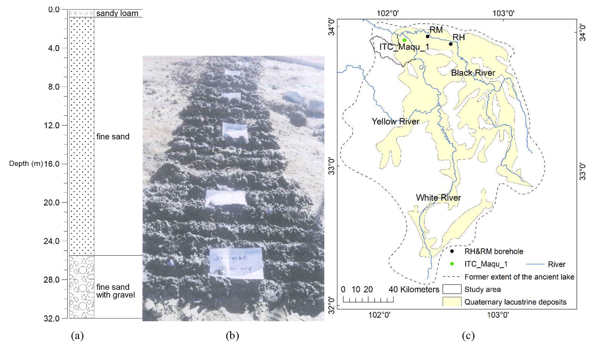
Figure 6Borehole information: (a) the core lithology of borehole ITC_Maqu_1, (b) a picture of the core sediment when the borehole was drilled, (c) location of boreholes RM and RH (after Chen et al., 1999).
4.2 Soil thickness measurement
Results of soil thickness measurements indicate that in the mountainous west, feldspathic quartzose sandstone and sandy slate parent materials show variable soil depths related to landscape position, i.e. the soil thicknesses decrease as the slope increases, and are within 1.2 m in most cases (Fig. 7a). Based on the measurements, the relationship between the soil thickness and slope can be expressed using the equation
where x is the slope (∘), and y is soil thickness (cm). Equation (9) is a regression line from data obtained over residual soils in the west. The measured thickness is a result of in situ soil-forming processes, while in the east, a transported soil is observed, the thickness of which is controlled by different processes from those acting on residual soils. In general, assuming similar geology and except for the valley bottom, Eq. (9) would apply to the western study area (Fig. 7b).
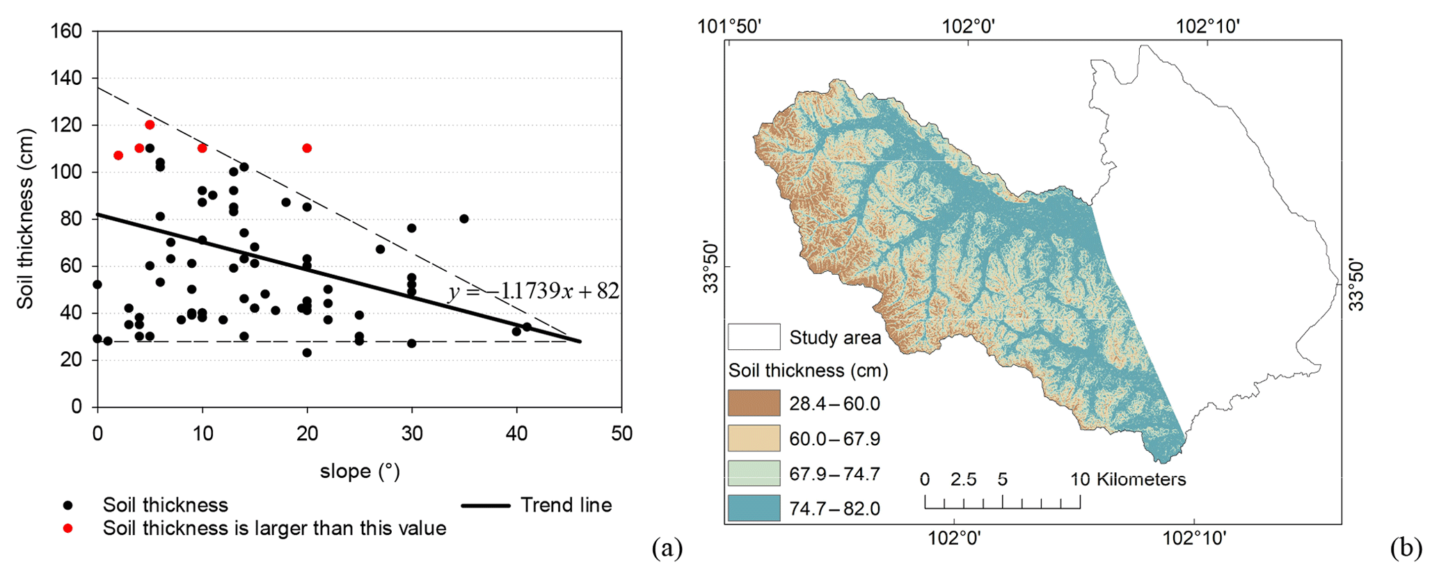
Figure 7Soil thickness: (a) soil thickness (cm) vs. slope (∘), (b) estimated soil thickness using Eq. (9).
In the west, under the soil layer, a less weathered layer exists where water can also flow and needs to be taken into account in the conceptual model. In the field, the difference between the less weathered layer and the soil layer is that the less weathered layer contains partially weathered stones. According to the owners of three boreholes located in or near the valley (numbered 32–34 in Fig. 8), their depths are larger than 10 m and do not reach bedrock. By subtracting the estimated soil thickness (Fig. 7b) from available depth-to-bedrock estimates, for example from Yan et al. (2020) and Shangguan et al. (2017), the thickness of the less weathered layer can be estimated (Fig. 8). In the mountainous west, because the estimated depth to bedrock is often at least an order of magnitude larger than the soil thickness, the uncertainty in the less weathered layer thickness mainly depends on the uncertainty in the estimated depth to bedrock, which is high due to the lack of boreholes for appropriate training (Shangguan et al., 2017; Yan et al., 2020).
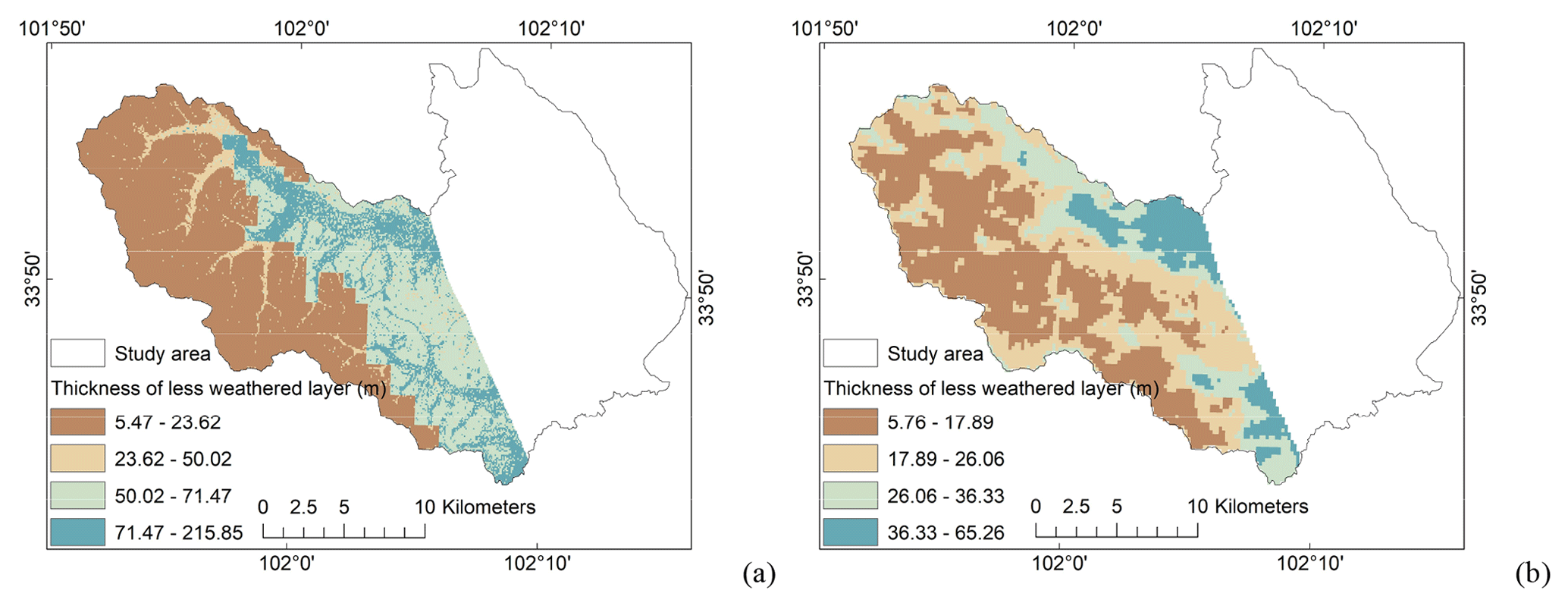
Figure 8The estimated thickness of the less weathered layer in the west: (a) based on the ensemble model estimated depth to bedrock from Yan et al. (2020), (b) based on the depth to bedrock from Shangguan et al. (2017).
According to the study from Yan et al. (2020), the ensemble-model-estimated depth to bedrock in the mountainous west ranges from 6.2 to 70.0 m, and in the east it is generally within the range of 70 to 95 m, while according to Shangguan et al. (2017), the depth to bedrock in the mountainous west ranges from 6.4 to 35.0 m and in the east is generally within the range of 35 to 74 m. Both studies appear to underestimate depth to bedrock in the east, which is also due to the lack of boreholes for proper constraining. Though with high uncertainty, the calculated less weathered layer thickness in the west can be applied for characterizing the hydrogeological conceptual model since the west mainly plays a role in collecting water, and there are no other data available to determine the thickness of the less weathered layer.
4.3 Hydrogeological surveys
4.3.1 Water table depth measurement
For the altitude survey, ALOS RT1, with a spatial resolution of 12.5 m, performed better than other DEM products across the whole study area and had a higher resolution than the others. It was the most suitable DEM to be used in this study area for determining water table (WT) depths. For details, see Appendix A1.
There were 22 WT depths measured in 2018 and 18 in 2019 (Fig. 3). In the flat eastern area, the WT depths were interpolated with the software Surfer (https://www.goldensoftware.com/products/surfer, last access: 4 March 2021) using the default ordinary kriging method with the linear variogram model (slope = 1, anisotropy ratio = 1, anisotropy angle = 0) (Cressie, 1990, 1991), which provides reasonable grids in most circumstances. Owing to the fact that most people living in the mountainous west use water from streams (via field survey), the need for groundwater is low, and only few boreholes exist. As such, only three boreholes numbered 32–34 were found in that western area (Fig. 9), and WT depths were measured. Normally, a good interpolation of WT depths or piezometric head over a large area needs and uses every measurement. But in this case, a reasonable WT depth map or piezometric head map in the mountainous west will need more than 100 borehole measurements (Hopkins and Anderson, 2016) because the ground surface elevation changes dramatically in the west, and so does the groundwater level. The three boreholes are far from enough to provide a reasonable WT depth map or piezometric head map and, therefore, were excluded from the interpolation. In contrast, the measured groundwater depths (and the interpolation) in the eastern study area can give a reasonable WT depth map or piezometric head map (Fig. 9a and b). Among the 34 boreholes with WT depth measurements, ground surface elevations measured by GPS-RTK were only available for 13 boreholes. For the remaining 21 boreholes, ground surface elevations were extracted from ALOS RT1. These elevations were used to derive hydraulic heads by subtracting the WT depths from the ground surface elevation. Similarly, using the kriging method, hydraulic heads were interpolated to obtain piezometric maps in the flat east (Fig. 9c and d).
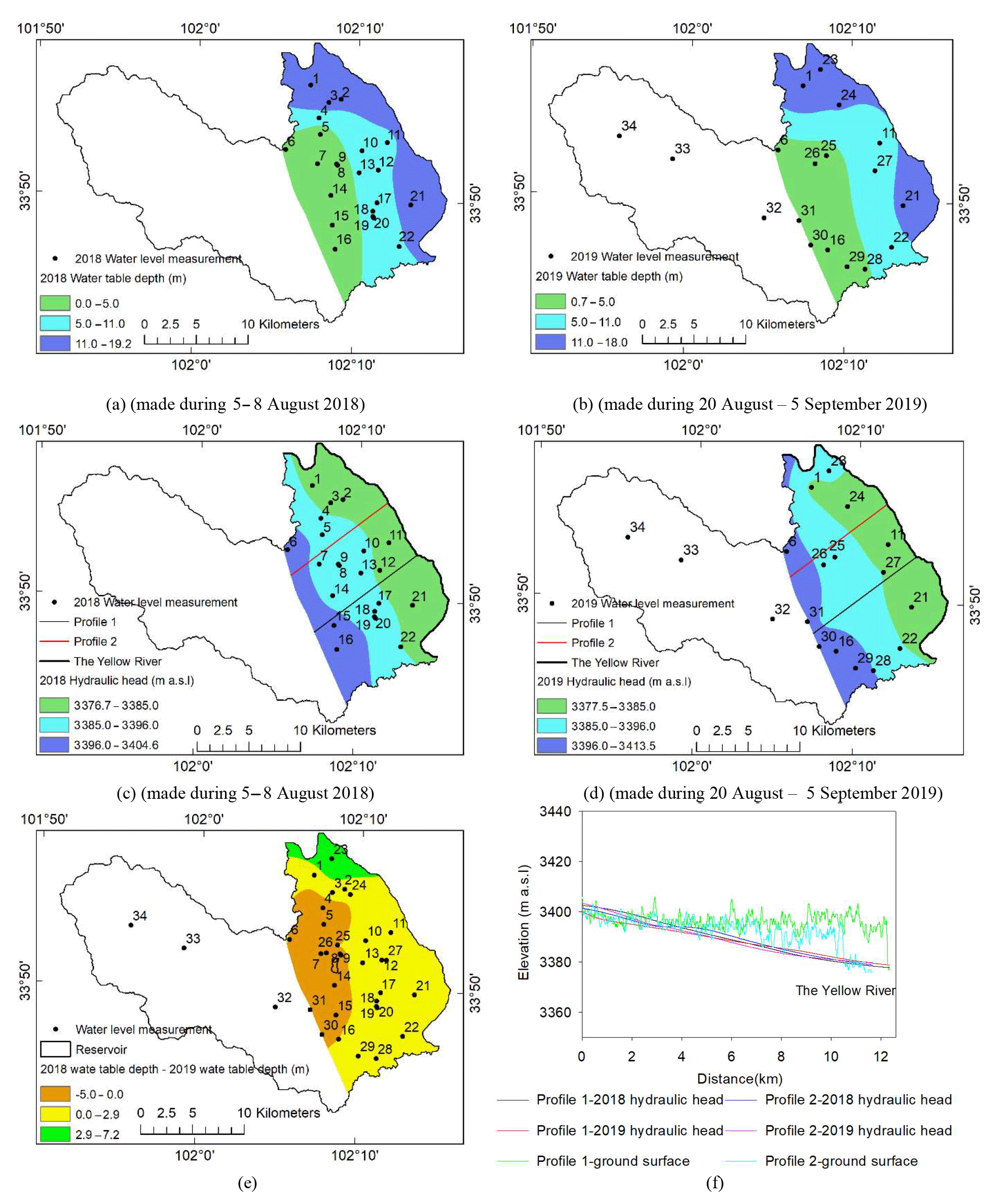
Figure 9Water table depths (m) and piezometric heads (m a.s.l.) of the eastern Maqu catchment. Panels (a) and (b) are water table depths (m) of the eastern Maqu catchment in 2018 and 2019, respectively; (c) and (d) are piezometric heads (m a.s.l.) of the eastern Maqu catchment in 2018 and 2019, respectively; (e) is the difference (m) in water table depth between 2018 and 2019; (f) is the profile 1 and profile 2 showing the hydraulic head and ground surface, with the profile locations shown in Fig. 9c and d. Numbers from 1 to 34 are identification numbers of boreholes.
In general, the range of WT depth was between 0.0 and 19.1 m in 2018 and between 0.7 and 18.0 m in 2019. In both 2018 and 2019, the interpolated WT depths (Fig. 9a and b) show a similar trend; i.e. the depth increases from the middle of the study area to the eastern boundary. The difference in WT depth in 2018 and 2019 (Fig. 9e) is probably caused by (1) different positions and number of control points, (2) the gates being open to reduce water storage in the reservoir (Fig. 9e) in 2019 to facilitate nearby constructions, (3) the interannual variation in precipitation and evapotranspiration. Nevertheless, in both 2018 and 2019, hydraulic heads (Fig. 9c and d) decrease from the middle of the study area to the eastern boundary, meaning that the groundwater flow is from the west to the east, with a hydraulic gradient of about 0.002 (dimensionless), recharging the Yellow River (Fig. 9f). This is consistent with the conclusion from Chang (2009). Ground surface elevations in Fig. 9f were extracted from ALOS RT1, and hydraulic heads were extracted from Fig. 9c and d. Some hydraulic heads are higher than the ground surface elevations as shown in Fig. 9f, which is due to (1) the accuracy of ALOS RT1 and (2) the lack of control points of hydraulic heads.
4.3.2 Aquifer tests
There were 11 aquifer tests conducted (Figs. 10 and 3) in unconfined aquifers, in partially penetrating boreholes. Eight slug tests were done in boreholes numbered 16, 21, 24, 26, 27, 32, 33, and 34 (Fig. 9); two pumping tests were carried out in 2019 at boreholes 6 and 23 (Fig. 9); and one pumping test was carried out in 2017 at the borehole ITC_Maqu_1. Data were processed automatically in AquiferTest software (https://www.waterloohydrogeologic.com/products/aquifertest/, last access: 4 March 2021) with assumptions made considering the average conditions in the study area: the aquifer is unconfined and 35 m thick; the borehole is partially penetrating; the screen radius is 0.27 m; the screen length is 15 m; the distance from aquifer top to screen bottom is 15 m; the casing radius is 0.25 m; the borehole radius is 0.3 m. Considering the spatial heterogeneity of hydraulic conductivities, they were not interpolated in the study area. As a result, the hydraulic conductivities ranged from 0.1 to 15.6 m d−1 (Fig. 10). According to Healy et al. (2007), this range of hydraulic conductivity can be classified as fine silty sand to coarse clean sand. The slug test in borehole 24 provided lower estimates of hydraulic conductivity than the nearby pumping test in borehole ITC_Maqu_1, which likely underestimated the hydraulic conductivity as borehole 24 was not used for a period of time. Therefore, compared to the slug test, the hydraulic conductivity obtained from the pumping test is more accurate and is a volumetric average, which makes it more suitable to calibrate Cp because MRS results are also volumetric averages.
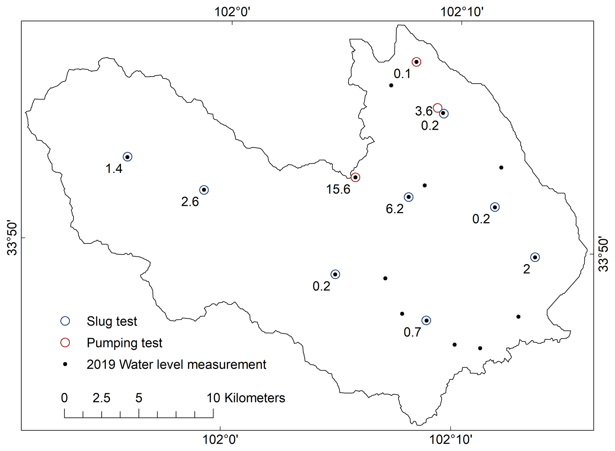
Figure 10Hydraulic conductivity (m d−1) obtained from aquifer tests in the Maqu catchment.
4.4 Hydrogeophysical surveys
4.4.1 MRS
ERT results were used to establish geoelectrical models for MRS inversion (see Appendix A3). The magnetic susceptibility measurements reveal very low susceptibility in the catchment, ensuring the suitability of applying MRS in the study area (see Appendix A2).
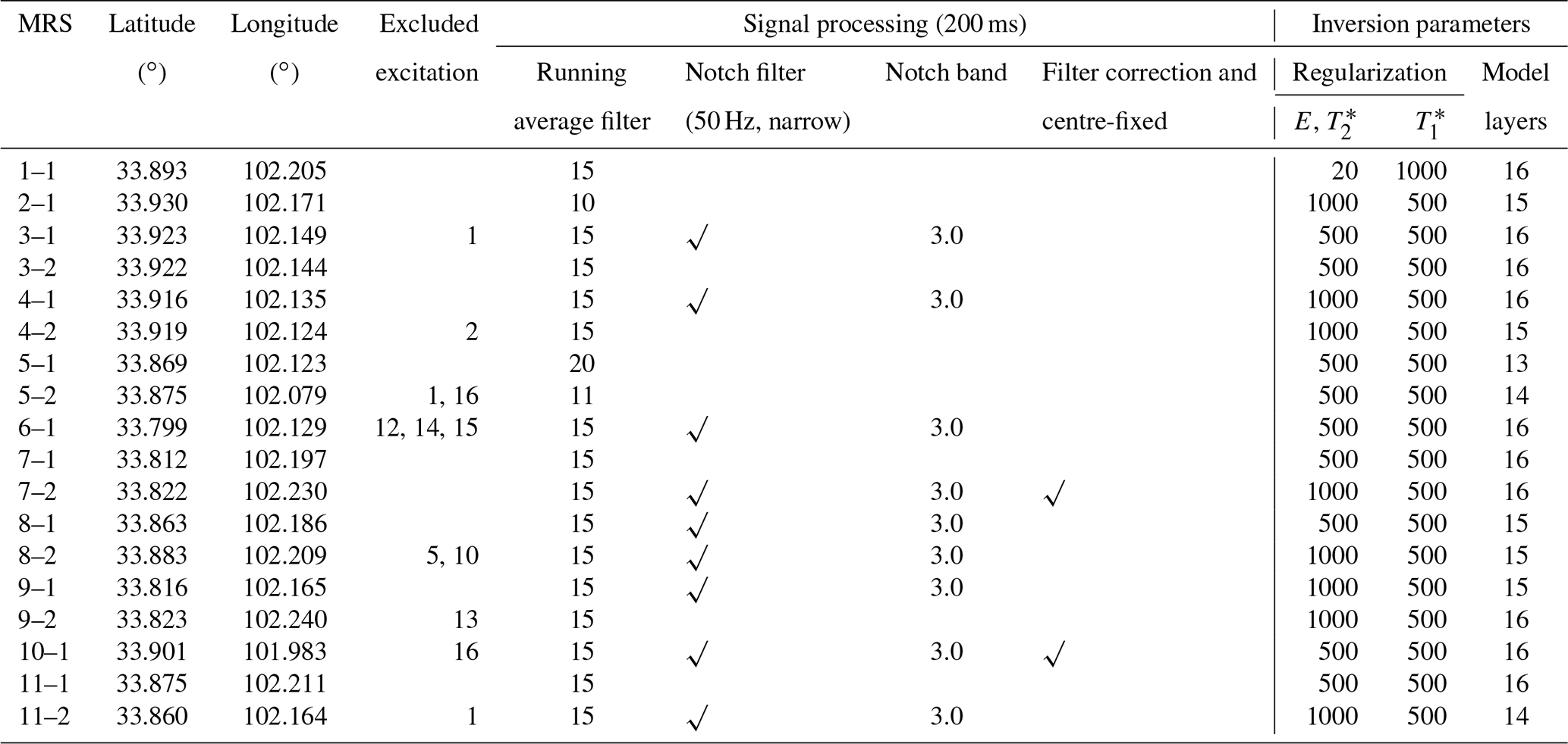
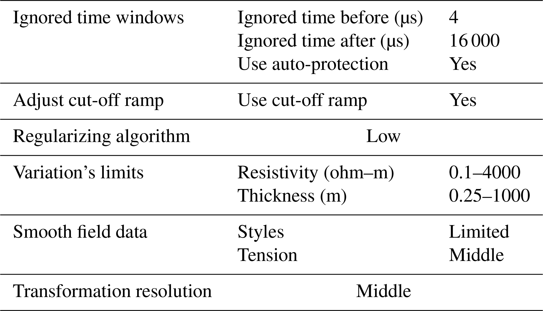
We did not use default inversion parameters because they sometimes result in abrupt changes or discontinuities of water content at two adjacent MRS sounding sites and lead to unrealistic results (Shah et al., 2008). Some excitations were excluded during inversion based on and the mismatch in terms of amplitude, Larmor frequency, and phase. The inversion parameters are listed in Table A7. The temperature of the water leads to different water densities and viscosities and therefore also influences hydraulic parameters. In Samovar V6.6, a default temperature of 20 ∘C is used. But in the study area, the average groundwater temperature is 6.2 ∘C. Therefore, it was necessary to take the true groundwater temperature into account when estimating hydraulic parameters. Thus, by correcting gravitational acceleration, water densities, and water viscosities using Eq. (10), a correction factor of 0.69 was used during the inversion process to improve accuracy.
where K is hydraulic conductivity (m d−1), k is the permeability of porous media (m2), ρ is water density (kg m−3), g is the gravitational acceleration (m s−2), and η is water viscosity (Pa s).
MRS3-1 sounding (Fig. 5) was used to calculate the calibration coefficient Cp because it is the nearest MRS sounding to the borehole ITC_Maqu_1 for which pumping test data are available. Using a single point of calibration, the calibration coefficient Cp can be estimated with the uncertainty ≤150 % (Boucher et al., 2009). The calibrated Cp is for T1 and for . Figure 11 shows inversion results of water content and T1 of MRS2-1, MRS3-1, and MRS3-2, and complete results are shown in Fig. A3 in the Appendix. Details are available in MRS inversion results.xlsx at the National Tibetan Plateau Data Center, including T1, , water content, T1- and -derived hydraulic conductivities and , and T1- and -derived transmissivities and .

The water content distribution of MRS9-2, MRS7-2, MRS7-1, and MRS4-1 (Fig. A3) extends down to 150 m deep. Except for MRS4-1, soundings MRS9-2, MRS7-2, and MRS7-1 are adjacent, indicating that in the south-east, near the Yellow River, the groundwater extends to more than 150 m depth. So it is concluded that the flat east plays the main role in storing groundwater, and the groundwater can extend to more than 150 m depth.
Limiting values of 0.00 and 1000.00 ms for and 0.00 and 3000.00 ms for T1 are indicators that a valid numerical solution to the measured records (i.e. the inversion) was not reached, and no valid outcome is available. Except for invalid values, T1-derived hydraulic conductivity () ranges from 0.00 to 210.98 m d−1, and -derived hydraulic conductivity () ranges from 0.00 to 19.64 m d−1. The value of 0.00 m d−1 comes from the estimation of very low water content. Here, an order-of-magnitude difference is observed between the range of and , which is due to the big difference between T1 and . In theory, T1 is less affected by magnetic heterogeneities and thus permits a better estimation of the hydraulic conductivity compared to . However, it is to note that no magnetic disturbance is expected in the Maqu catchment (Fig. A1). Furthermore in the case of T1, because two timed delayed responses are compounded, any model mismatch, e.g. the MRS loop sampled volume being significantly different from a layered model parallel to the loop due to near-source river deposit media heterogeneity, can make the measured responses “doubly” distorted and may not fit a T1 expected response. In both cases, T1 and , a distortion is occurring. Nevertheless, according to specific circumstances, , which is evaluated from rest with a single pulse, may undergo less severe overall distortion. So and tend to be more reliable than and and should be used for future study. By checking the values of , it is concluded that there is an unconfined aquifer in the eastern study area. Based on (and water content results), with a proper threshold to define aquifer and non-aquifer, the aquifer geometry can be defined.
MRS has its own limitations in that some of the in situ water information is missing and that the current “window of the technique” is only sensitive to the larger pore fraction of water content. The near-source river environment leads to the unknown mixture of varied lithology. Missing water is unknown, but accounting for a variety of lithology, including fine-pore lithology, from water table depth (Fig. 9) to the base of the aquifer (50 to 208 m range; see the following TEM section) may lead to well over 50 % missed water (Boucher et al., 2011). Besides, the invalid values for and T1 may be attributed to the hydrogeological conditions, such as highly heterogeneous lithology or too-low signal-to-noise ratio, and may be eased using an updated version of Samovar V6.6, such as Samovar V11.4, which not only improves the capability of signal analysis, for example, and allows the optimization of the number of inverted layers but also adds an uncertainty estimation function by incorporating singular value decomposition. Nevertheless, in highly heterogeneous environments, the indetermination of some parameters may remain with current technology. In terms of using default inversion parameters, part of the difficulty is in fitting the observed data to a too-large number of layers: i.e. partly fitting to the noise component of the records. The heterogeneity of the near-source river environment is also contributing to this difficulty. With more recent tools, like Samovar V11.4, the difficulty can be better handled (Legchenko et al., 2017).
In general, MRS provides preliminary and valuable information on water content, hydraulic conductivity, and transmissivity. Once the geometrical mapping and its fabric have been mapped, groundwater flow parameters and groundwater storage or volume can be better determined.
4.4.2 TEM
A variety of acquisition parameters were applied, and the signals were analysed to determine the optimal TEM measurements for each site. Detailed information of 10 optimal TEM measurements and inversion parameters is listed in Tables 3 and A8, respectively. The industrial noise filter was set at 50 Hz, and the amplifier was off. In the study area, using the square loop with a side length of 48 m or 95 m, the maximum time of 1 ms or 4 ms, stack between 5–10, and current of 0.8 A or 1.1 A, the TEM method can reach the maximum investigation depth ranging from 150 to more than 1000 m. For data processing, the invalid data points were first removed, and the field data were smoothed. Then the voltage data were inverted to obtain an apparent resistivity, which was further inverted to get true resistivity (Abiye and Haile, 2008; Cosentino et al., 2007). Applying a variety of acquisition parameters ensures that bad data can be revealed (Auken et al., 2006). Induced polarization (IP) and superparamagnetic (SPM) effects were not considered in the inversion process (Macnae, 2016). Because of the dead time and the fact that at most sites, a relatively dry layer of sediments exists near the ground surface with a corresponding high-resistivity depth interval, the upper 15 to 30 m of the sounding is lost, although subsequent layered Earth modelling attempts fill the gap.
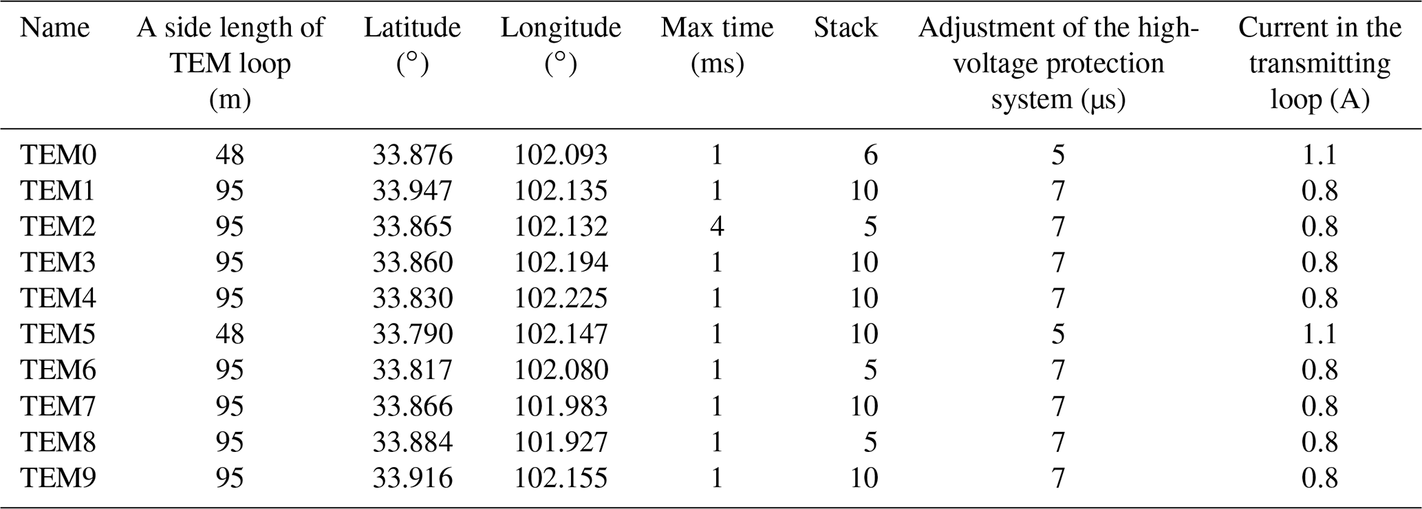
The root mean square (RMS) error in the inversion results shown in Fig. 12 is below 2 % in the flat area and below 10 % in the mountainous area. The results in the mountainous area, i.e. results of TEM6, TEM7, and TEM8, indicate that the resistivity becomes larger in the deep subsurface and is consistent with our understanding that the bedrock is located at relatively shallow depth from the ground surface. The maximum investigation depth of TEM6 is shallow; only 10 time windows were available and resulted in about 150 m investigation depth from the ground surface. This may be due to the local unknown geological condition. In addition to consolidated rock resistivity of the order of 2 to 4 kΩ m, TEM7 and TEM8 responses may show instances of fracturing, weathering, or faulting. To determine exactly what structure it is and the scope of the structure, further investigation is needed, for example, a systematic high-spatial-resolution geophysical survey with appropriate depth capability, such as the airborne electromagnetic survey, followed by systematic borehole drilling. The rest of the TEM measurements are scattered in the east, where it is likely that lake deposits are covered by river deposits on the top. Because the clay silt lithology has a lower resistivity than sand-rich lithology, and Chen et al. (1999) suggested that the ancient lake in Ruoergai basin was a freshwater or slightly saline lake for most of its life, the decrease in resistivity may indicate the change from river deposits to lake deposits. Table 4 listed the TEM-derived depth of the bottom of river deposits in the east. For TEM0, TEM1, TEM2, TEM3, TEM4, and TEM9, the bottoms of river deposits are deeper than 100 m, with lake deposits underneath. But for TEM5, located near the mountainous area, the bottom of river deposits is at 50 m deep, followed by 64 m thick lake deposits, with the bedrock at the bottom, and the nearest MRS sounding MRS6-1 indeed shows that there is no free water under 50 m depth.
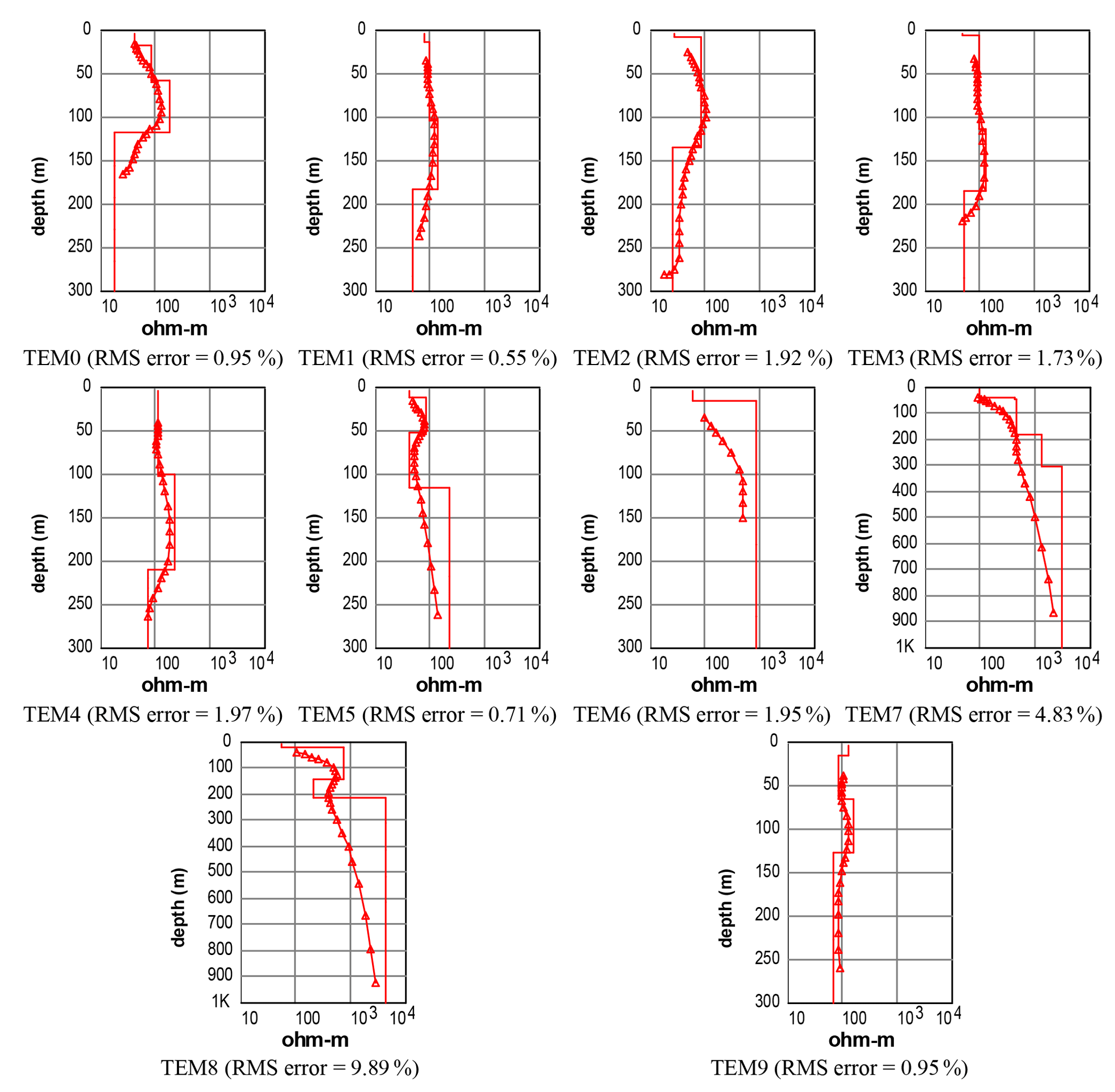
Figure 12Apparent resistivity with depth. The red triangles connected by the red line represent the measured apparent resistivity values, and the red line without triangles represents the inverted 1-D geoelectric model.
Table 4TEM-derived depth of river deposits bottom in the east.

The large contact area between river and lake deposits in the eastern study area and the Ruoergai basin allows large water exchange. According to Fig. 12, the thickness of the lake deposits can reach more than 150 m. The thick lake deposits constitute a nearly infinite hydraulic buffer reservoir, allowing multi-year storage equivalent in the Maqu catchment. Thus it would be relevant to include the deep lake deposits in future hydrogeological models.
4.5 Uncertainties
As shown in Fig. 2, direct techniques, i.e. particle size analysis, altitude survey, soil thickness measurement, water table depth measurement, aquifer test, and magnetic susceptibility measurements, have low uncertainties. There are random errors for particle size analysis (Wang, 2011), but they are small and not expected to affect the final lithology result (ASTM D6913/D6913M-17, 2017) and thus can be neglected. For measured ground surface elevations, soil thicknesses, and water table depths, the uncertainty is supposed to be within a few centimetres considering the accuracy of equipment and errors during the measurement process (Burt, 2014; Cunningham and Schalk, 2011; Rydlund Jr. and Densmore, 2012). In terms of hydraulic heads derived from ALOS RT1 in boreholes, the uncertainty comes not only from water table depth measurement but also from ALOS RT1, which contains the mean absolute error of 4.4 m in the study area based on our results (Table A1). For hydraulic conductivities obtained from aquifer tests, the uncertainty mainly comes from data collection and processing. Though the duration of pumping in the borehole ITC_Maqu_1 did not reach 48 h, the water levels became steady very soon after the pumping started, so the uncertainty is estimated to be within 25 % according to studies from Brown et al. (1995) and Delnaz et al. (2019). For magnetic susceptibility, although the resolution of SM–20 is SI units, the actual reading accuracy is dependant on appropriate corrections, e.g. temperature, shape, volume, effective distance to sensor, etc. The corrections may reach a few orders of magnitude for volume and up to % for shape (Hoffman, 2006). In the case of the Maqu catchment, these are so far from the levels at which the MRS problem may occur that, corrected or not, the final results will still be below the threshold for concerns.
In terms of indirect techniques, ERT, MRS, and TEM, performances of the raw data could be evaluated with parameters such as for MRS and number of bad data for ERT and TEM. Knowledge of the subsurface geometry and fabric would lead to the resolution of the main uncertainty issues for inverted data because there are implicit modelling assumptions for each method. For example, the assumption for MRS is that the subsurface is made of 1D planar layers parallel to the MRS loop with depth-increasing thickness. We cannot quantify the extent to which these assumptions are met and therefore also the extent to which the inversion data are accurate measurements of the site's hydrogeological parameters; thus appropriate uncertainty figures cannot be reliably generated for inverted data. The inverted data, as an illustration of what can be extracted from the raw data, are preliminary results with only inversion RMS errors quantified (ERT and TEM). Lake deposits, being far from the source, should not suffer from the near-source river deposits' heterogeneity, but their lithology makes it insensitive to MRS.
To further reduce uncertainties from indirect techniques, ERT, MRS, and TEM, it is important to determine subsurface geometry and its fabric. State-of-the-art airborne electromagnetic technology allows high-spatial-resolution mapping down to 500 m depth and is probably the most appropriate tool for now (Legault, 2015). After the site geometry is properly mapped, and the subsurface fabric is properly understood, optimum borehole drilling locations can be selected. When the detailed geometrical mapping of the subsurface and systematic borehole information are available, the inversion process can be better constrained and improved (Galazoulas et al., 2015; Vouillamoz et al., 2005; Wang et al., 2021).
The raw dataset is archived and freely available in the DANS repository under the link https://doi.org/10.17026/dans-z6t-zpn7 (Li et al., 2020a), and the dataset containing the processed ERT, MRS, and TEM data is available at the National Tibetan Plateau Data Center with the link https://doi.org/10.11888/Hydro.tpdc.271221 (Li et al., 2020b).
We conducted borehole core lithology analysis, an altitude survey, soil thickness measurement, hydrogeological surveys, and hydrogeophysical surveys in the Maqu catchment of the Yellow River source region on the Tibetan Plateau, where little subsurface data are available. Seven DEMs were evaluated using GPS-RTK-measured ground surface elevations, and ALOS RT1 is suggested to be used in this study because of its better accuracy as well as higher resolution than other DEMs. The medium-deep lithology of the subsurface down to 32 m below the ground surface, mainly composed of sand, is available from one borehole (ITC_Maqu_1). It helps provide useful information for the cross-validation with hydrogeophysical survey results. According to the in situ measurements, soil thicknesses, except on the valley floor, are within 1.2 m depth in most cases in the west, and the soil thickness decreases as the slope increases. The hydrogeological surveys reveal that groundwater flows from the west to the east, recharging the Yellow River, and the hydraulic conductivity ranges from 0.2 to 12.4 m d−1. The hydrogeophysical surveys demonstrate the presence of an unconfined aquifer in the east. The water content and hydraulic parameters of that aquifer were estimated at MRS sounding locations. The depth of the Yellow River deposits was derived at TEM sounding positions in the flat eastern area.
Although water table depths were only measured once or twice, and hydrogeophysical methods, like ERT, TEM, and MRS, have inherent non-uniqueness problems during the inversion process, they all provide valuable information, especially in such data-scarce areas as the TP. The data from direct techniques with low uncertainties, as shown in Fig. 2 (lithology, ground surface elevation, soil thickness, water table depth measurement, hydraulic conductivity from aquifer test, magnetic susceptibility), can contribute to related global or regional databases where the in situ data over the TP are scarce or be regarded as verification and validation data for groundwater modelling over the Maqu catchment. Indirect techniques such as ERT, MRS, and TEM are a rare, unique, and particularly rich training data source for geoscientists interested in the data processing and interpretation of the particular hydrogeological and hydrogeophysical techniques used here. It is a dynamic set where additional complementary data will gradually add constraints to the inversion processes. For example, a researcher developing new techniques for improvements of some of these techniques will get free and highly relevant data to work with.
In the Maqu catchment, a near-source river environment without adequate geometrical mapping, the representativity of the various sampled volumes is unknown as well as whether the sampled volume fits the models used for data inversion. This is much less the case farther away from the source where homogeneity and fitting of the model to the actual hydrogeological setting are achieved. In such an away-from-source case, pumping test data may be assumed to be representative of the tested formation, while in techniques such as MRS, depth and thickness information may be extracted from the datasets as well as hydraulic estimates. This is an ongoing project, and it may become available later if such above-mentioned mapping is completed. Any further similar surveys and borehole drillings would benefit from such geometrical mapping since their precise localization may then be optimized in view of proper data inversion and information gap filling.
Generally speaking, all the methods work well in the study area and have confirmed the presence of an unconfined fluvial aquifer within the 250 m below the surface and the presence of lake deposits with much finer pore lithology. By combining our dataset with available depth-to-bedrock datasets, a preliminary hydrogeological conceptual model can be established. If combining our dataset with detailed geometrical mapping of the subsurface and deep borehole information, a more complete and accurate conceptual model can be obtained. Furthermore, we will be monitoring the groundwater and surface water in the study area and aim for establishing a long-term monitoring network, which will eventually contribute to the verification and validation of future studies on groundwater modelling over the Maqu catchment. To our knowledge, this is the first time such detailed surveys were conducted in a TP catchment in order to set up a hydrogeological conceptual and numerical groundwater model. This paper is expected not only to contribute to the hydrogeological conceptual and numerical model of the Maqu catchment at the TP but also to provide data for hydrogeological and hydrogeophysical communities and promote interdisciplinary research.
A1 Altitude survey
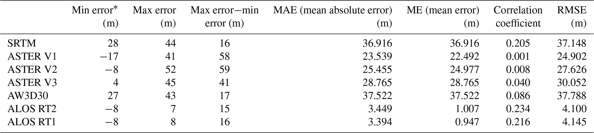
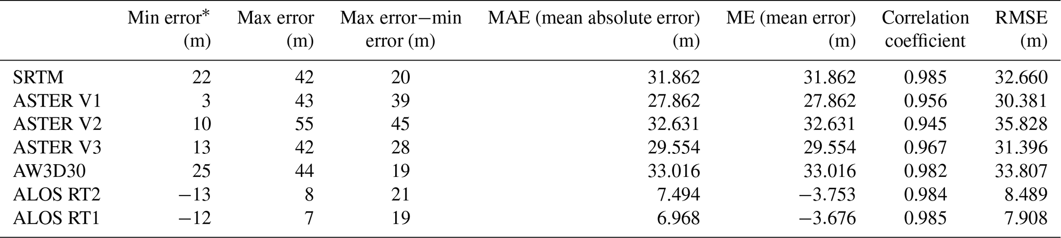
A total of 46 ground surface elevations were measured (33 in the flat east, 13 in the mountainous west) and were used to evaluate the accuracies of seven DEM datasets (data available in DEM.xlsx in the National Tibetan Plateau Data Center), and the most accurate one was applied in this study. The statistical analysis results of the seven DEMs in the study area are shown in Table A1. The root mean square errors (RMSEs) of ALOS RT1 and ALOS RT2 are 5.695 and 5.477 m, respectively, much smaller than the RMSE of the other five DEMs. The correlation coefficient, the mean error, and the mean absolute errors in ALOS RT1 and ALOS RT2 also show better performance than those of the other five DEMs. Comparing ALOS RT1 with ALOS RT2, ALOS RT1 slightly outperforms ALOS RT2 with regards to RMSE, correlation coefficient, and the mean error. Tables A2 and A3 list the statistical analysis results of seven DEMs separately for the flat eastern area and the mountainous western area. All seven DEMs behave better in the west than the east in terms of the correlation coefficient. In the west, the correlation coefficients of seven DEMs are all larger than 0.94, while in the east, the correlation coefficients are all lower than 0.24. This is because the range of ground surface elevation in the flat east is much smaller than the range of elevation in the mountainous west. With regard to the RMSE, mean error, and mean absolute error, all seven DEMs have better behaviour in the east than in the west. In general, ALOS RT1 and ALOS RT2 also outperform the other five DEMs, according to Tables A2 and A3.
Since ALOS RT1 performs slightly better than ALOS RT2 in the whole study area and has a higher resolution than ALOS RT2, it is the most suitable DEM to use in this study area. For ALOS RT1 in the flat east, 52 % of errors (DEM value − GPS-RTK value) are within the range of −3 to 3 m, and 79 % of errors are within the scope of −5 to 5 m, while in the mountainous west, 54 % of errors are within the range of −8 to −12 m, and 46 % of errors are within the range of 0 to 7 m.
Previous TP works about DEM evaluation mainly focused on SRTM and ASTER. Our results are generally consistent with previous studies in terms of RMSE of SRTM. Nan et al. (2015) evaluated the height accuracy of SRTM and ASTER in the eastern TP with reference to the relatively high precision of the 1:50 000 scale DEM surveyed and mapped by the State Bureau of Surveying and Mapping in China. As a result, the RMSEs of SRTM and ASTER are 35.3 and 50.2 m, respectively. Ye et al. (2011) evaluated SRTM and ASTER in the Mt. Qomolangma (Mt. Everest) area on the TP by comparing 211 elevation checkpoints on the 1:50 000 topographic maps surveyed and mapped by the State Bureau of Surveying and Mapping in China, demonstrating an average height difference of 31.3 and 44.9 m for SRTM and ASTER, respectively. However, there are other studies that have different evaluation results. Fujita et al. (2008) found that the elevation differences between DEMs and ground survey data from differential GPS were 11.0 m for ASTER and 11.3 m for SRTM in the Lunana region, Bhutan Himalaya. The DEM evaluation results also indicated that in different places over the TP, the satellite DEM estimates are acquired with varying accuracy. This may be due to different topographic complexity in different areas.
The DEMs' quality can be influenced by several factors, such as sensor type, algorithm, terrain type, and grid spacing (Hebeler and Purves, 2009). In this study, grid spacings of DEMs are similar except for ALOS RT1, so the main factors that affect the accuracy of the DEMs should be sensor types and algorithms. For SRTM, the issue inherent to the production method is mast oscillations, while for ASTER and AW3D30, the issue is scene mismatch (Grohmann, 2018). As for radiometrically terrain-corrected (RTC) products ALOS RT1 and ALOS RT2, the quality is directly related to the quality of the source DEM SRTM which was used in the RTC process. This results in very similar correlation coefficients of SRTM, ALOS RT1, and ALOS RT2 and obvious improvements in RMSE, MAE, and ME (Table A1).
Table A1Statistical analysis of seven DEMs in the study area.

* Error = DEM value−GPS-RTK value.
Table A2Statistical analysis of seven DEMs in the flat eastern area.
* Error = DEM value−GPS-RTK value.
Table A3Statistical analysis of seven DEMs in the mountainous western area.
* Error = DEM value−GPS-RTK value.
A2 Magnetic susceptibility
The magnetic susceptibility measurements (Fig. A1) reveal very low susceptibility in the catchment, with susceptibility values all smaller than SI units, with an average of SI units. A previous study from Chen et al. (1999) also reported low magnetic susceptibility of the RH core (Fig. 6c) with 120 m length located 40 km east of the study area in the Ruoergai basin. The low magnetic susceptibility ensured the suitability of applying MRS in the study area.
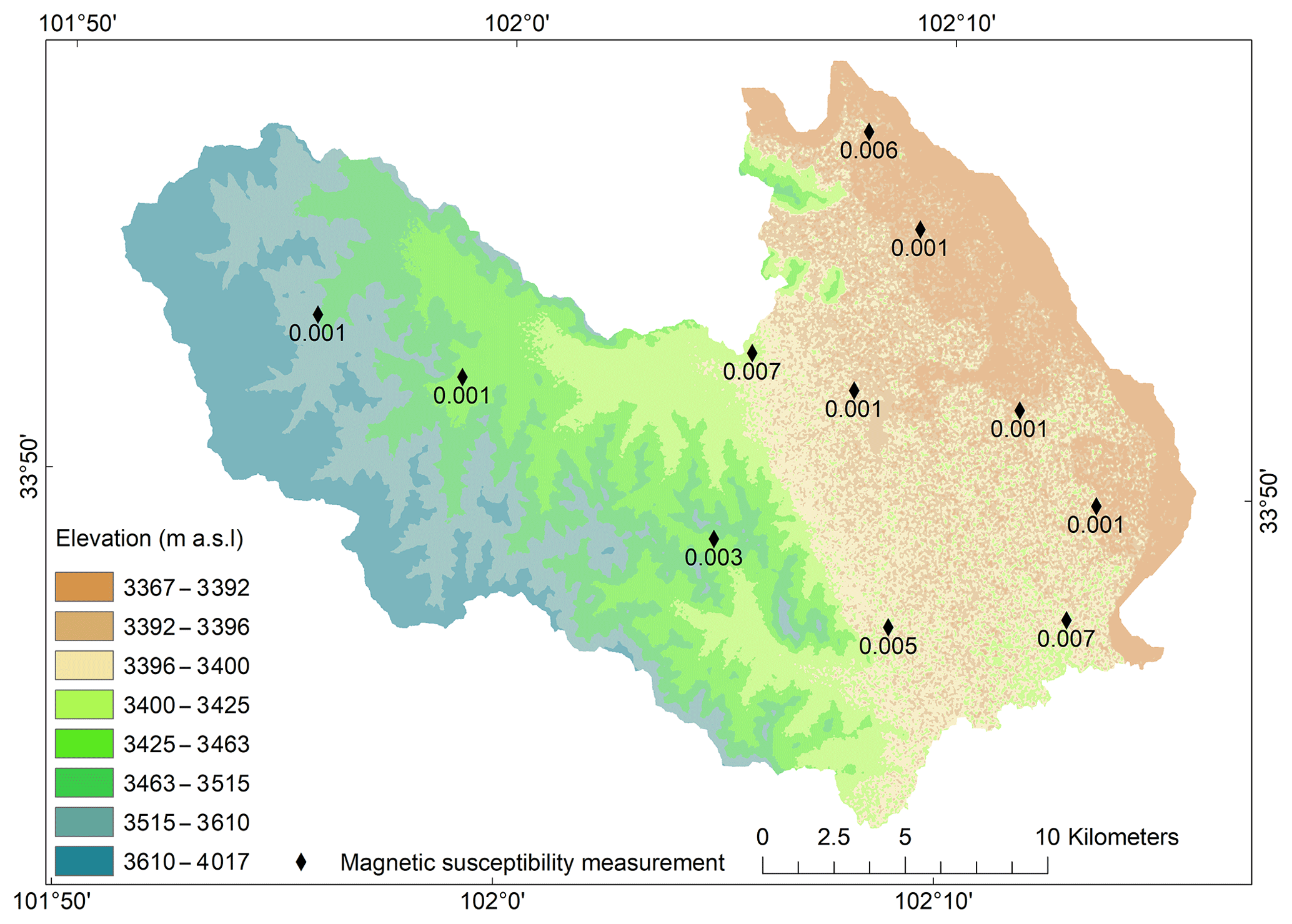
Figure A1Magnetic susceptibility measurements (10−3 SI units) ensured the suitability of applying MRS in the study area.
A3 ERT
Detailed information of ERT profiles and inversion parameters is listed in Tables A4 and A5, respectively. For a specific pseudo-depth, the values between adjacent points generally vary smoothly. Bad data points can be easily identified as they appeared as outlier points in the pseudo-section plot in RES2DINV due to their too-high or too-low apparent resistivity values. The bad data points were filtered out based on the following criteria: (i) having negative apparent resistivity or small apparent resistivity close to 0 Ω m or (ii) having negative or positive pulse amplitude ratios <0.75 or >1.33 (a measure of waveform symmetry) (Slater et al., 2010; Wilkinson et al., 2016). After filtering, the least square method was used for the inversion. Results are shown in Fig. A2, with the root mean square (RMS) error less than 5 %. A pattern of roughly regular parallel-to-surface electrostratigraphy is observed in all ERT profiles, except 0–310 m of profile ERT5, where the pattern is dipping relative to the surface. This means that strata are likely to be stratified in most parts of the study area. For ERT2, ERT3, ERT5, and ERT6, three electrostratigraphic layers can be identified: the first layer with the highest resistivity, the second layer with the lowest resistivity, and the third layer with a medium resistivity. The second layer is likely to represent an aquifer. However, considering ERT4 and ERT7, there is a lack of marker electrostratum; i.e. a layer with high resistivity does not exist at the ground surface. This is probably due to high water content near the ground surface in the mountainous area where ERT4 and ERT7 were located. As for ERT1, rainfall occurred during the field measurement. Rainwater accumulations occurred next to some of the electrodes, causing abnormal current distribution during the ERT measurements, and about half of the data were filtered out. The ERT1 inversion results show a three-layer pattern similar to the one observed along the ERT2, ERT3, ERT5, and ERT6 profiles. One or more short-wavelength anomalies (<200 m) are observed along all profiles but particularly in the case of ERT1, ERT3, and ERT6. Short-wavelength anomalies along ERT1 may be due to data acquisition made during rainfall, while in the case of the other profiles, localized changes in water content or lithology variations are suspected.
Compared to the dipole–dipole configuration, the investigation depth of the Wenner configuration is deeper. So resistivity values obtained from the Wenner configuration were used to establish geoelectrical models for MRS inversion. For ERT2, ERT3, ERT5, and ERT6, three-layer geoelectrical models were extracted, while for ERT4 and ERT7, two-layer geoelectrical models were extracted. ERT1 was neglected due to the influence of rainfall. For ERT5, from 0 to 310 m, there is a topographic change; the ground surface elevation decreases from 3395 m a.s.l. and stabilizes at around 3390 m a.s.l. Ground surface with low resistivity exists along this 310 m transect. Because the MRS soundings were conducted in flat areas, only resistivity from 310 to 810 m was used for the first layer of the geoelectrical model. The geoelectrical models and corresponding MRS measurements are shown in Table A6. The depths of the last layer of geoelectrical models are extended to 1.5 times the MRS investigation depth since signal distortion due to subsurface resistivity is calculated down to that depth while making the MRS linear filter. In this particular version, MRS investigation depth was considered to be the MRS loop size, i.e. 150 and 100 m. Nevertheless, like other geophysical methods, ERT has equivalence problems, i.e. non-uniqueness of inversion results. Despite equivalence problems, the ERT method still provides important subsurface information in the Maqu catchment, where we have little fundamental information. This is the very first investigation in this area; when more lithology information becomes available later, ERT can be better constrained to reflect the subsurface lithology.
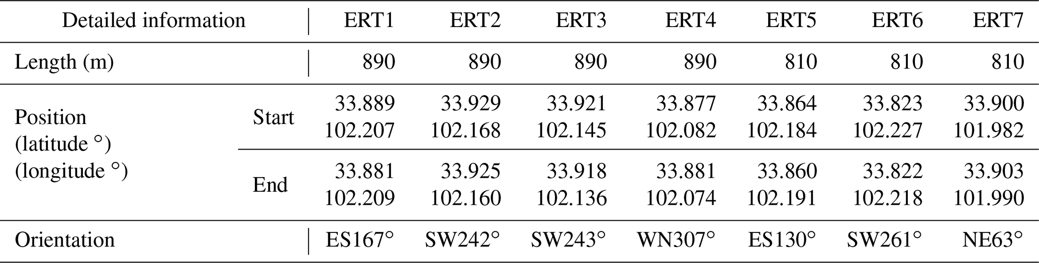
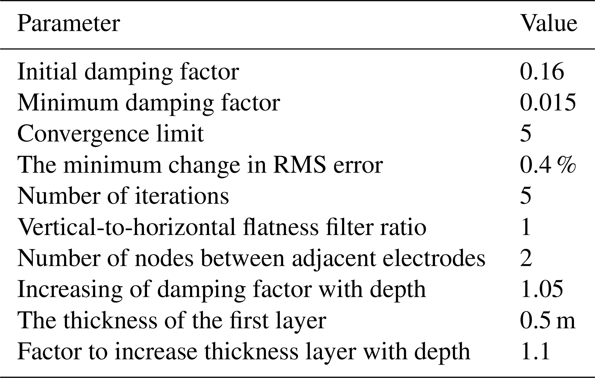
Table A6Geoelectrical models used for MRS inversion.
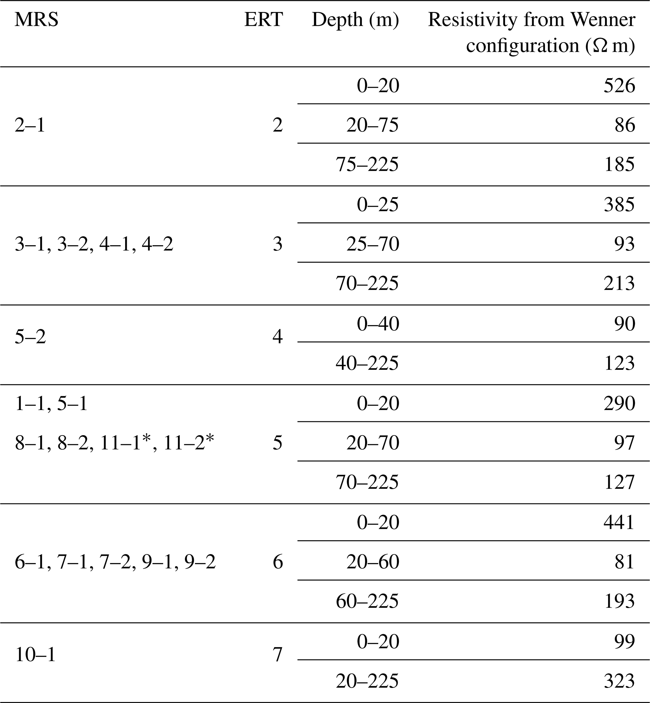
* The depth of the third layer is 150 m rather than 225 m.
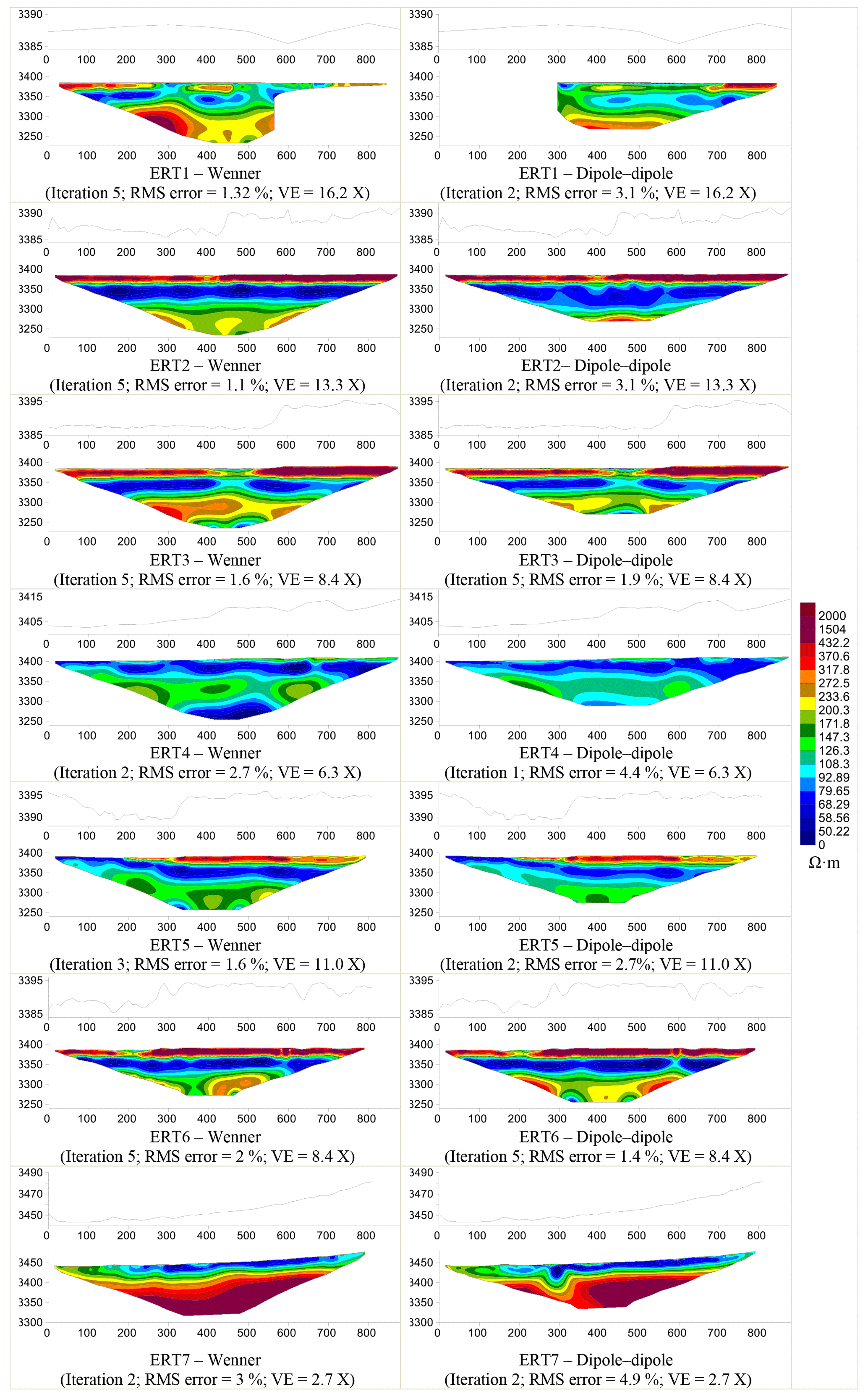
Figure A2ERT measurements and corresponding ground surface elevation and vertical exaggeration (VE).
A4 Inversion parameters for MRS
A5 MRS inversion results
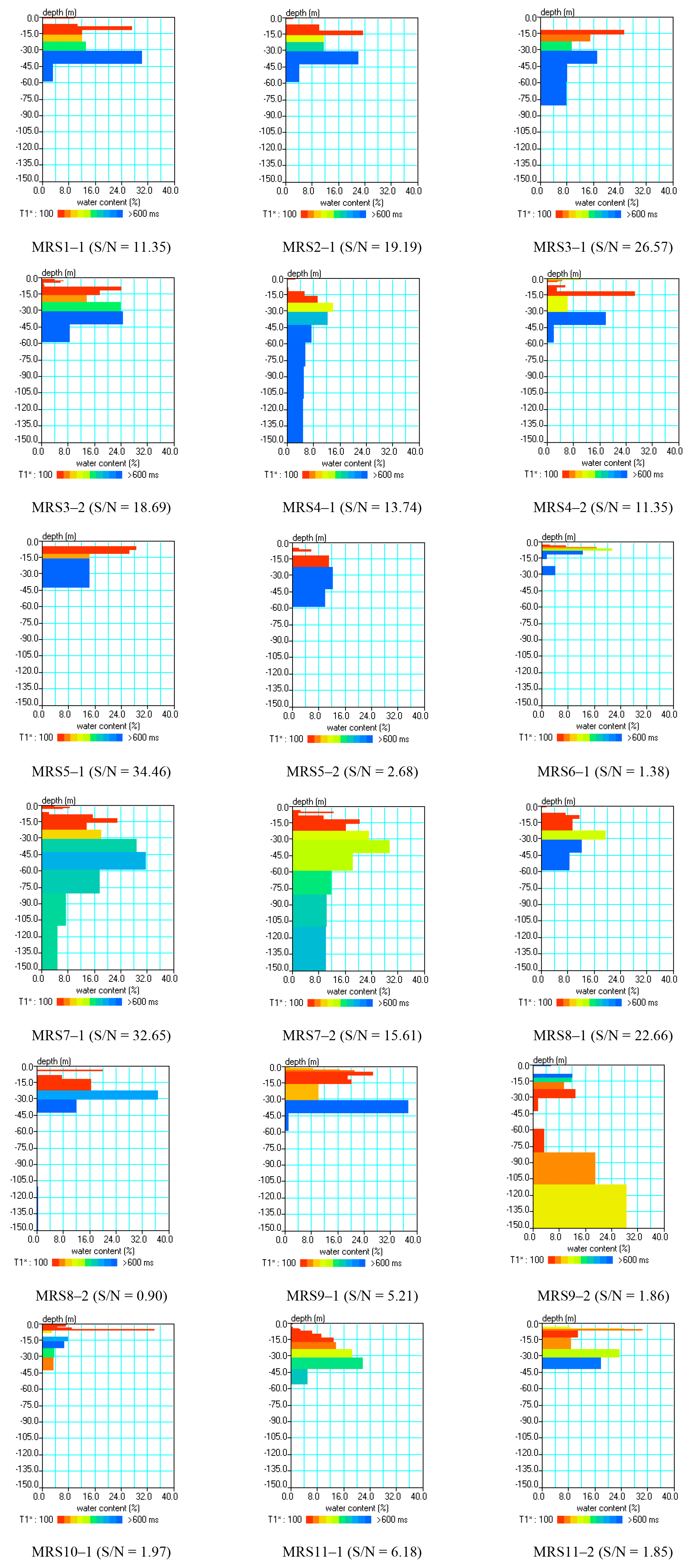
Figure A3Water content and T1 derived from MRS measurements.
A6 TEM inversion parameters
A7 Abbreviations
| ALOS PALSAR RT1 | Advanced Land Observing Satellite – Phase Array type L-band Synthetic Aperture Radar – high terrain correction resolution |
|---|---|
| ALOS PALSAR RT2 | Advanced Land Observing Satellite – Phase Array type L-band Synthetic Aperture Radar – low terrain correction resolution |
| AMSR-E | Advanced Microwave Scanning Radiometer for Earth Observing System |
| ASCAT | Advanced Scatterometer |
| ASF | Alaska Satellite Facility |
| ASTER | The Terra Advanced Spaceborne Thermal Emission and Reflection Radiometer |
| CAS | Chinese Academy of Science |
| CLM | Community Land Model |
| CPC | Climate Prediction Center |
| DEM | Digital elevation model |
| ERT | Electrical Resistivity Tomography |
| GDEM | Global digital elevation model |
| GLDAS | Global Land Data Assimilation System |
| GPS | Global positioning system |
| GPS-RTK | Real-time kinematic global positioning system |
| GRACE | Gravity Recovery and Climate Experiment |
| JAXA | Japan Aerospace Exploration Agency |
| LAPSUS | LandscApe ProcesS modeling at mUlti-dimensions and scaleS |
| ME | Mean error |
| MAE | Mean absolute error |
| MRI | Magnetic resonance imaging |
| MRS | Magnetic resonance sounding |
| NMR | Nuclear magnetic resonance |
| RMSE | Root mean square error |
| SRTM | Shuttle Radar Topography Mission |
| TDEM | Time domain electromagnetic |
| TEM | Transient Electromagnetic |
| TP | Tibetan Plateau |
| USGS | United States Geological Survey |
| VIC | Variable Infiltration Capacity model |
| WT | Water table |
| YRSR | Yellow River source region |
The supplement related to this article is available online at: https://doi.org/10.5194/essd-13-4727-2021-supplement.
ML, ZS, YZ, MWL, JR, LY, HQ, ZL, JC, LH, HZ, TV, JMS, and HJHF contributed to the design of this research. ML, JR, LY, HQ, ZL, JC, KH, QZ, PX, FL, KL, and YL carried out the fieldwork. All co-authors revised the manuscript and contributed to the writing.
The authors declare that they have no conflict of interest.
Publisher’s note: Copernicus Publications remains neutral with regard to jurisdictional claims in published maps and institutional affiliations.
This article is part of the special issue “Extreme environment datasets for the three poles”. It is not associated with a conference.
We thank Mark van der Meijde from the University of Twente, the staff of the Maqu Water Authority, and Yongming Yang of Hequ stud farm for their great support for fieldwork.
This research has been supported by the Second Tibetan Plateau Scientific Expedition and Research (STEP) programme (grant no. 2019QZKK0103), the National Natural Science Foundation of China (grant nos. 41971033, 32071586, 20 41931285, 41790441, 41572236, and 42102288), the ESA MOST Dragon IV programme (Monitoring and Modelling Climate Change in Water, Energy and Carbon Cycles in the Pan-Third Pole Environment), the Fundamental Research Funds for the Central Universities (grant nos. 300102298307, 25 300102299305, 300102291507, 300102291402, 300102291401, and 300102291105), the Programme of Introducing Talents of Discipline to Universities (grant no. B08039), and the Natural Science Foundation of Shaanxi Province (grant no. 2020JQ-349).
This paper was edited by David Carlson and reviewed by two anonymous referees.
Abiye, T. A. and Haile, T.: Geophysical exploration of the Boku geothermal area, Central Ethiopian Rift, Geothermics, 37, 586–596, 2008.
Agarwal, R. G.: A new method to account for producing time effects when drawdown type curves are used to analyze pressure buildup and other test data, SPE Paper 9289 presented at the 55th SPE Annual Technical Conference and Exhibition, Dallas, Texas, 21–24 September 1980, https://doi.org/10.2118/9289-MS, 1980.
ASTM D6913/D6913M-17: Standard Test Methods for Particle-Size Distribution (Gradation) of Soils Using Sieve Analysis, ASTM International, West Conshohocken, PA, 2017, https://doi.org/10.1520/D6913_D6913M-17, 2017.
Auken, E., Pellerin, L., Christensen, N. B., and Sørensen, K.: A survey of current trends in near-surface electrical and electromagnetic methods, Geophysics, 71, G249–G260, 2006.
Bernard, J.: Instruments and field work to measure a magnetic resonance sounding, Boletin Geologico y Minero, 118, 459–472, 2007.
Boucher, M., Favreau, G., Vouillamoz, J.-M., Nazoumou, Y., and Legchenko, A.: Estimating specific yield and transmissivity with magnetic resonance sounding in an unconfined sandstone aquifer (Niger), Hydrogeol. J., 17, 1805, https://doi.org/10.1007/s10040-009-0447-x, 2009.
Boucher, M., Costabel, S., and Yaramanci, U.: The detectability of water by NMR considering the instrumental dead time–A laboratory analysis of unconsolidated materials, Near Surf. Geophys., 9, 145–154, 2011.
Boulton, N. S.: Analysis of data from non-equilibrium pumping tests allowing for delayed yield from storage, Proc. Inst. Civil Eng., 26, 469–482, https://doi.org/10.1680/iicep.1963.10409, 1963.
Bouwer, H. and Rice, R.: A slug test for determining hydraulic conductivity of unconfined aquifers with completely or partially penetrating wells, Water Resour. Res., 12, 423–428, https://doi.org/10.1029/WR012i003p00423, 1976.
Braun, M. and Yaramanci, U.: Inversion of resistivity in magnetic resonance sounding, J. Appl. Geophys., 66, 151–164, https://doi.org/10.1016/j.jappgeo.2007.12.004, 2008.
Brown, D. L., Narasimhan, T., and Demir, Z.: An evaluation of the Bouwer and Rice method of slug test analysis, Water Resour. Res., 31, 1239–1246, 1995.
Burt, R.: Soil survey field and laboratory methods manual, United States Department of Agriculture, Natural Resources Conservation Service, National Soil Survey Center, Kellogg Soil Survey Laboratory, Lincoln, Nebraska, 2014.
Chambers, J., Wilkinson, P., Uhlemann, S., Sorensen, J., Roberts, C., Newell, A., Ward, W., Binley, A., Williams, P., and Gooddy, D.: Derivation of lowland riparian wetland deposit architecture using geophysical image analysis and interface detection, Water Resour. Res., 50, 5886–5905, https://doi.org/10.1002/2014WR015643, 2014.
Chang, D. Z.: Preliminary analysis and research on the Yellow River water resources in Maqu wetland, Gansu Water Conservancy and Hydropower Technology, 45, 8–10, 2009.
Chen, F., Bloemendal, J., Zhang, P., and Liu, G.: An 800 ky proxy record of climate from lake sediments of the Zoige Basin, eastern Tibetan Plateau, Palaeogeogr. Palaeoclimatol. Palaeoecol., 151, 307–320, 1999.
Chirindja, F. J., Dahlin, T., Perttu, N., Steinbruch, F., and Owen, R.: Combined electrical resistivity tomography and magnetic resonance sounding investigation of the surface-water/groundwater interaction in the Urema Graben, Mozambique, Hydrogeol. J., 24, 1583–1592, https://doi.org/10.1007/s10040-016-1422-y, 2016.
Compton, R. R.: Manual of field geology, Wiley, New York, 1962.
Cosentino, P., Capizzi, P., Fiandaca, G., Martorana, R., Messina, P., and Pellerito, S.: Study and monitoring of salt water intrusion in the coastal area between Mazara del Vallo and Marsala (South-Western Sicily), in: Methods and Tools for Drought Analysis and Management, Springer, Netherlands, 2007.
Cressie, N.: The origins of kriging, Math. Geol., 22, 239–252, 1990.
Cressie, N.: Statistics for spatial data, John Wiley & Sons, New York, 1991.
Cunningham, W. L. and Schalk, C. W.: Groundwater technical procedures of the US Geological Survey, US Geological Survey Techniques and Methods 151 pp., 2011.
Dackombe, R. and Gardiner, V.: Geomorphological field manual, Routledge, London, 270 pp., 2020.
Delnaz, A., Rakhshandehroo, G., and Nikoo, M. R.: Optimal estimation of unconfined aquifer parameters in uncertain environment based on fuzzy transformation method, Water Supply, 19, 444–450, 2019.
Dente, L., Vekerdy, Z., Wen, J., and Su, Z.: Maqu network for validation of satellite-derived soil moisture products, Int. J. Appl. Earth Obs. Geoinf., 17, 55–65, https://doi.org/10.1016/j.jag.2011.11.004, 2012.
Descloitres, M., Séguis, L., Wubda, M., and Legchenko, A.: Discrimination of rocks with different hydrodynamic properties using MRS, EM and resistivity methods, Near Surface 2007-13th EAGE European Meeting of Environmental and Engineering Geophysics, 2007.
Descloitres, M., Ruiz, L., Sekhar, M., Legchenko, A., Braun, J. J., Mohan Kumar, M., and Subramanian, S.: Characterization of seasonal local recharge using electrical resistivity tomography and magnetic resonance sounding, Hydrol. Process., 22, 384–394, https://doi.org/10.1002/hyp.6608, 2008.
Di Napoli, R., Aiuppa, A., Sulli, A., Caliro, S., Chiodini, G., Acocella, V., Ciraolo, G., Di Vito, M., Interbartolo, F., and Nasello, C.: Hydrothermal fluid venting in the offshore sector of Campi Flegrei caldera: A geochemical, geophysical, and volcanological study, Geochem. Geophy. Geosy., 17, 4153–4178, https://doi.org/10.1002/2016GC006494, 2016.
Fan, Y. and Van Den Dool, H.: Climate Prediction Center global monthly soil moisture data set at 0.5 resolution for 1948 to present, J. Geophys. Res.-Atmos., 109, D10102, https://doi.org/10.1029/2003JD004345, 2004.
Fan, Y., Li, H., and Miguez-Macho, G.: Global patterns of groundwater table depth, Science, 339, 940–943, 2013.
Fikos, I., Vargemezis, G., Zlotnicki, J., Puertollano, J., Alanis, P., Pigtain, R., Villacorte, E., Malipot, G., and Sasai, Y.: Electrical resistivity tomography study of Taal volcano hydrothermal system, Philippines, Bull. Volcanol., 74, 1821–1831, https://doi.org/10.1007/s00445-012-0638-5, 2012.
Fujita, K., Suzuki, R., Nuimura, T., and Sakai, A.: Performance of ASTER and SRTM DEMs, and their potential for assessing glacial lakes in the Lunana region, Bhutan Himalaya, J. Glaciol., 54, 220–228, 2008.
Galazoulas, E. C., Mertzanides, Y. C., Petalas, C. P., and Kargiotis, E. K.: Large scale electrical resistivity tomography survey correlated to hydrogeological data for mapping groundwater salinization: a case study from a multilayered coastal aquifer in Rhodope, Northeastern Greece, Environmental processes, 2, 19–35, 2015.
Gao, S., Jin, H., Bense, V. F., Wang, X., and Chai, X.: Application of electrical resistivity tomography for delineating permafrost hydrogeology in the headwater area of Yellow River on Qinghai-Tibet Plateau, SW China, Hydrogeol. J., 27, 1725–1737, https://doi.org/10.1007/s10040-019-01942-z, 2019.
Gleeson, T., Smith, L., Moosdorf, N., Hartmann, J., Dürr, H. H., Manning, A. H., van Beek, L. P., and Jellinek, A. M.: Mapping permeability over the surface of the Earth, Geophys. Res. Lett., 38, L02401, https://doi.org/10.1029/2010GL045565, 2011.
Gleeson, T., Moosdorf, N., Hartmann, J., and Van Beek, L.: A glimpse beneath earth's surface: GLobal HYdrogeology MaPS (GLHYMPS) of permeability and porosity, Geophys. Res. Lett., 41, 3891–3898, 2014.
Gleeson, T., Befus, K. M., Jasechko, S., Luijendijk, E., and Cardenas, M. B.: The global volume and distribution of modern groundwater, Nat. Geosci., 9, 161–167, 2016.
Gonçalves, R. M. D.: Hydrochemical water prediction (water quality) with transient electromagnetic soundings (TEM), PhD thesis, University of Lisbon, Lisbon, Portugal, 314 pp., 2012.
Graham, D. N. and Butts, M. B.: Flexible integrated watershed modelling with MIKE SHE, in: Watershed models, edited by: Singh, V. P. and Frevert, D. K., CRC Press, Boca Raton, Florida, 245–272, 2005.
Grohmann, C. H.: Evaluation of TanDEM-X DEMs on selected Brazilian sites: Comparison with SRTM, ASTER GDEM and ALOS AW3D30, Remote Sens. Environ., 212, 121–133, 2018.
Gupta, S., Hengl, T., Lehmann, P., Bonetti, S., and Or, D.: SoilKsatDB: global database of soil saturated hydraulic conductivity measurements for geoscience applications, Earth Syst. Sci. Data, 13, 1593–1612, https://doi.org/10.5194/essd-13-1593-2021, 2021.
Haile, K. H.: Estimation of terrestrial water storage in the upper reach of Yellow River, University of Twente Faculty of Geo-Information and Earth Observation (ITC), Enschede, Netherlands, 2011.
Healy, R. W., Winter, T. C., LaBaugh, J. W., and Franke, O. L.: Water budgets: foundations for effective water-resources and environmental management, US Geological Survey Reston, Virginia, 2007.
Hebeler, F. and Purves, R. S.: The influence of elevation uncertainty on derivation of topographic indices, Geomorphology, 111, 4–16, 2009.
Herckenrath, D., Auken, E., Christiansen, L., Behroozmand, A. A., and Bauer-Gottwein, P.: Coupled hydrogeophysical inversion using time-lapse magnetic resonance sounding and time-lapse gravity data for hydraulic aquifer testing: Will it work in practice?, Water Resour. Res., 48, W01539, https://doi.org/10.1029/2011WR010411, 2012.
Hoffman, R. E.: Measurement of magnetic susceptibility and calculation of shape factor of NMR samples, J. Magn. Reson., 178, 237–247, 2006.
Hopkins, J. and Anderson, B.: A Field Manual for Groundwater-level Monitoring at the Texas Water Development Board, User Manual 52, 26 pp., available at: https://www.twdb.texas.gov/groundwater/docs/UMs/UM-52.pdf (last access: 4 March 2021), 2016.
Huang, X., Deng, J., Wang, W., Feng, Q., and Liang, T.: Impact of climate and elevation on snow cover using integrated remote sensing snow products in Tibetan Plateau, Remote Sens. Environ., 190, 274–288, https://doi.org/10.1016/j.rse.2016.12.028, 2017.
Immerzeel, W. W., Droogers, P., De Jong, S., and Bierkens, M.: Large-scale monitoring of snow cover and runoff simulation in Himalayan river basins using remote sensing, Remote Sens. Environ., 113, 40–49, https://doi.org/10.1016/j.rse.2008.08.010, 2009.
Immerzeel, W. W., Van Beek, L. P., and Bierkens, M. F.: Climate change will affect the Asian water towers, Science, 328, 1382–1385, https://doi.org/10.1126/science.1183188, 2010.
Jiang, F., Dong, L., and Dai, Q.: Electrical resistivity imaging inversion: An ISFLA trained kernel principal component wavelet neural network approach, Neural Networks, 104, 114–123, https://doi.org/10.1016/j.neunet.2018.04.012, 2018.
Jiao, J. J., Zhang, X., Liu, Y., and Kuang, X.: Increased water storage in the Qaidam Basin, the North Tibet Plateau from GRACE gravity data, PloS one, 10, e0141442, https://doi.org/10.1371/journal.pone.0141442, 2015.
Kang, S., Xu, Y., You, Q., Flügel, W.-A., Pepin, N., and Yao, T.: Review of climate and cryospheric change in the Tibetan Plateau, Environ. Res. Lett., 5, 015101, https://doi.org/10.1088/1748-9326/5/1/015101, 2010.
Kenyon, W., Howard, J., Sezginer, A., Straley, C., Matteson, A., Horkowitz, K., and Ehrlich, R.: Pore-size distribution and NMR in microporous cherty sandstones, SPWLA 30th Annual Logging Symposium, Denver, Colorado, 11–14 June 1989.
Kuang, X. and Jiao, J. J.: Review on climate change on the Tibetan Plateau during the last half century, J. Geophys. Res.-Atmos., 121, 3979–4007, https://doi.org/10.1002/2015JD024728, 2016.
Lachassagne, P., Baltassat, J.-M., Legchenko, A., and de Gramont, H. M.: The links between MRS parameters and the hydrogeological parameters, Near Surf. Geophys., 3, 259–265, https://doi.org/10.3997/1873-0604.2005021, 2005.
Legault, J. M.: Airborne electromagnetic systems – state of the art and future directions, CSEG Recorder, 40, 38–49, 2015.
Legchenko, A., Baltassat, J.-M., Beauce, A., and Bernard, J.: Nuclear magnetic resonance as a geophysical tool for hydrogeologists, J. Appl. Geophys., 50, 21–46, https://doi.org/10.1016/S0926-9851(02)00128-3, 2002.
Legchenko, A., Baltassat, J. M., Bobachev, A., Martin, C., Robain, H., and Vouillamoz, J. M.: Magnetic resonance sounding applied to aquifer characterization, Groundwater, 42, 363–373, https://doi.org/10.1111/j.1745-6584.2004.tb02684.x, 2004.
Legchenko, A., Comte, J.-C., Ofterdinger, U., Vouillamoz, J.-M., Lawson, F. M. A., and Walsh, J.: Joint use of singular value decomposition and Monte-Carlo simulation for estimating uncertainty in surface NMR inversion, J. Appl. Geophys., 144, 28–36, 2017.
Legchenko, A., Miège, C., Koenig, L. S., Forster, R. R., Miller, O., Solomon, D., Schmerr, N., Montgomery, L., Ligtenberg, S., and Brucker, L.: Estimating water volume stored in the south-eastern Greenland firn aquifer using magnetic-resonance soundings, J. Appl. Geophys., 150, 11–20, https://doi.org/10.1016/j.jappgeo.2018.01.005, 2018.
Legchenko, A. V. and Shushakov, O. A.: Inversion of surface NMR data, Geophysics, 63, 75–84, https://doi.org/10.1190/1.1444329, 1998.
Li, M., Zeng, Y., Lubczynski, M. W., Su, Z., and Qian, H.: 2018–2019 dataset in Maqu, the Tibetan Plateau, DANS [data set], https://doi.org/10.17026/dans-z6t-zpn7, 2020a.
Li, M., Zeng, Y., Lubczynski, M., Su, Z., and Qian, H.: Multi dimensional observation data set of single watershed in Maqu County, Qinghai Tibet Plateau (2018–2019), TPDC Data Center [data set], https://doi.org/10.11888/Hydro.tpdc.271221, 2020b.
Li, X., Liu, S., Xiao, Q., Ma, M., Jin, R., Che, T., Wang, W., Hu, X., Xu, Z., and Wen, J.: A multiscale dataset for understanding complex eco-hydrological processes in a heterogeneous oasis system, Sci. Data, 4, 170083, https://doi.org/10.1038/sdata.2017.83, 2017.
Li, X., Gou, X., Wang, N., Sheng, Y., Jin, H., Qi, Y., Song, X., Hou, F., Li, Y., and Zhao, C.: Tightening ecological management facilitates green development in the Qilian Mountains, Chinese Sci. Bull., 64, 2928–2937, 2019.
Li, X., Che, T., Li, X., Wang, L., Duan, A., Shangguan, D., Pan, X., Fang, M., and Bao, Q.: CASEarth poles: big data for the three poles, B. Am. Meteorol. Soc., 101, E1475–E1491, 2020.
Li, X., Cheng, G., Wang, L., Wang, J., Ran, Y., Che, T., Li, G., He, H., Zhang, Q., and Jiang, X.: Boosting geoscience data sharing in China, Nat. Geosci., 14, 541–542, 2021.
Li, Z. and Gao, P.: Channel adjustment after artificial neck cutoffs in a meandering river of the Zoige basin within the Qinghai-Tibet Plateau, China, Catena, 172, 255–265, 2019.
Loke, M. H.: Electrical imaging surveys for environmental and engineering studies, User's Manual for Res2dinv, available at: https://www.academia.edu/11991713/Electrical (last acces: 8 August 2021), 1999.
Lubczynski, M. and Roy, J.: Hydrogeological interpretation and potential of the new magnetic resonance sounding (MRS) method, J. Hydrol., 283, 19–40, https://doi.org/10.1016/S0022-1694(03)00170-7, 2003.
Lubczynski, M. and Roy, J.: Magnetic resonance sounding: New method for ground water assessment, Groundwater, 42, 291–309, https://doi.org/10.1111/j.1745-6584.2004.tb02675.x, 2004.
Lubczynski, M. and Roy, J.: Use of MRS for hydrogeological system parameterization and modeling, Boletin Geologico y Minero, 118, 509–530, 2007.
Macnae, J.: Quantitative estimation of intrinsic induced polarization and superparamagnetic parameters from airborne electromagnetic data, Geophysics, 81, E433–E446, 2016.
McClymont, A. F., Roy, J. W., Hayashi, M., Bentley, L. R., Maurer, H., and Langston, G.: Investigating groundwater flow paths within proglacial moraine using multiple geophysical methods, J. Hydrol., 399, 57–69, https://doi.org/10.1016/j.jhydrol.2010.12.036, 2011.
McCormack, T., O'Connell, Y., Daly, E., Gill, L., Henry, T., and Perriquet, M.: Characterisation of karst hydrogeology in Western Ireland using geophysical and hydraulic modelling techniques, J. Hydrol. Reg. Stud., 10, 1–17, https://doi.org/10.1016/j.ejrh.2016.12.083, 2017.
Montzka, C., Herbst, M., Weihermüller, L., Verhoef, A., and Vereecken, H.: A global data set of soil hydraulic properties and sub-grid variability of soil water retention and hydraulic conductivity curves, Earth Syst. Sci. Data, 9, 529–543, https://doi.org/10.5194/essd-9-529-2017, 2017.
Nabighian, M. N. and Macnae, J. C.: Time domain electromagnetic prospecting methods, Electromagnetic Methods in Applied Geophysics, 2, 427–509, 1991.
Nan, X., Li, A., Bian, J., and Zhang, Z.: Comparison of the accuracy between SRTM and ASTER GDEM over typical mountain area: A case study in the Eastern Qinghai-Tibetan Plateau, J. Geo-Inf. Sci, 17, 91–98, https://doi.org/10.3724/SP.J.1047.2015.00091, 2015.
Nielsen, M. R., Hagensen, T. F., Chalikakis, K., and Legchenko, A.: Comparison of transmissivities from MRS and pumping tests in Denmark, Near Surf. Geophys., 9, 211–223, https://doi.org/10.3997/1873-0604.2010071, 2011.
Niu, F., Yin, G., Luo, J., Lin, Z., and Liu, M.: Permafrost distribution along the Qinghai-Tibet Engineering Corridor, China using high-resolution statistical mapping and modeling integrated with remote sensing and GIS, Remote Sens., 10, 215, https://doi.org/10.3390/rs10020215, 2018.
Peel, M. C., Finlayson, B. L., and McMahon, T. A.: Updated world map of the Köppen-Geiger climate classification, Hydrol. Earth Syst. Sci., 11, 1633–1644, https://doi.org/10.5194/hess-11-1633-2007, 2007.
Pérez-Bielsa, C., Lambán, L. J., Plata, J. L., Rubio, F. M., and Soto, R.: Characterization of a karstic aquifer using magnetic resonance sounding and electrical resistivity tomography: a case-study of Estaña Lakes (northern Spain), Hydrogeol. J., 20, 1045–1059, https://doi.org/10.1007/s10040-012-0839-1, 2012.
Plata, J. and Rubio, F.: Basic theory of the magnetic resonance sounding method, Boletin Geologico y minero, 118, 441–458, 2007.
Plata, J. L. and Rubio, F. M.: The use of MRS in the determination of hydraulic transmissivity: The case of alluvial aquifers, J. Appl. Geophys., 66, 128–139, https://doi.org/10.1016/j.jappgeo.2008.04.001, 2008.
Qu, B., Zhang, Y., Kang, S., and Sillanpaa, M.: Water quality in the Tibetan Plateau: Major ions and trace elements in rivers of the “Water Tower of Asia”, Sci. Total Environ., 649, 571–581, https://doi.org/10.1016/j.scitotenv.2018.08.316, 2019.
Rodell, M., Houser, P., Jambor, U., Gottschalck, J., Mitchell, K., Meng, C.-J., Arsenault, K., Cosgrove, B., Radakovich, J., and Bosilovich, M.: The global land data assimilation system, B. Am. Meteorol. Soc., 85, 381–394, 2004.
Roy, J., Rouleau, A., Chouteau, M., and Bureau, M.: Widespread occurrence of aquifers currently undetectable with the MRS technique in the Grenville geological province, Canada, J. Appl. Geophys., 66, 82–93, https://doi.org/10.1016/j.jappgeo.2008.04.006, 2008.
Rydlund Jr., P. H. and Densmore, B. K.: Methods of practice and guidelines for using survey-grade global navigation satellite systems (GNSS) to establish vertical datum in the United States Geological Survey, U.S. Geological Survey, Reston, Virginia, 102 pp., 2012.
Schoorl, J., Veldkamp, A., and Bouma, J.: Modeling water and soil redistribution in a dynamic landscape context, Soil Sci. Soc. Am. J., 66, 1610–1619, 2002.
Schoorl, J., Claessens, L., Lopez Ulloa, M., De Koning, G., and Veldkamp, A.: Geomorphological analysis and scenario modelling in the Noboa–Pajan area, Manabi province, Ecuador, Z. Geomorphol., 145, 105–118, 2006.
Seevers, D.: A nuclear magnetic method for determining the permeability of sandstones, SPWLA 7th Annual Logging Symposium, Tulsa, Oklahoma, 9–11 May 1966.
Shah, S. D., Kress, W. H., and Legchenko, A.: Application of Magnetic Resonance Soundings and Other Surface Geophysical Methods to Enhance Subsurface Analysis of a Ground-Water Availability Model – A Pilot Study, Symposium on the Application of Geophysics to Engineering and Environmental Problems 2008, Philadelphia, Pennsylvania, 896–915, 6–10 April 2008.
Shangguan, W., Hengl, T., de Jesus, J. M., Yuan, H., and Dai, Y.: Mapping the global depth to bedrock for land surface modeling, J. Adv. Model Earth Sy., 9, 65–88, https://doi.org/10.1002/2016MS000686, 2017.
Slater, L. D., Ntarlagiannis, D., Day-Lewis, F. D., Mwakanyamale, K., Versteeg, R. J., Ward, A., Strickland, C., Johnson, C. D., and Lane Jr., J. W.: Use of electrical imaging and distributed temperature sensing methods to characterize surface water–groundwater exchange regulating uranium transport at the Hanford 300 Area, Washington, Water Resour. Res., 46, W10533, https://doi.org/10.1029/2010WR009110, 2010.
Steelman, C., Kennedy, C., and Parker, B.: Geophysical conceptualization of a fractured sedimentary bedrock riverbed using ground-penetrating radar and induced electrical conductivity, J. Hydrol., 521, 433–446, https://doi.org/10.1016/j.jhydrol.2014.12.001, 2015.
Su, Z., Wen, J., Dente, L., van der Velde, R., Wang, L., Ma, Y., Yang, K., and Hu, Z.: The Tibetan Plateau observatory of plateau scale soil moisture and soil temperature (Tibet-Obs) for quantifying uncertainties in coarse resolution satellite and model products, Hydrol. Earth Syst. Sci., 15, 2303–2316, https://doi.org/10.5194/hess-15-2303-2011, 2011.
Su, Z., De Rosnay, P., Wen, J., Wang, L., and Zeng, Y.: Evaluation of ECMWF's soil moisture analyses using observations on the Tibetan Plateau, J. Geophys. Res.-Atmos., 118, 5304–5318, https://doi.org/10.1002/jgrd.50468, 2013.
Su, Z., Wen, J., Zeng, Y., Zhao, H., Lv, S., van der Velde, R., Zheng, D., Wang, X., Wang, Z., and Schwank, M.: Multiyear in-situ L-band microwave radiometry of land surface processes on the tibetan Plateau, Sci. Data, 7, 317 pp., 2020.
Thorne, P. and Newcomer, D.: Prototype database and User's guide of saturated zone hydraulic properties for the Hanford site, in: Report PNNL-14058, Pacific Northwest National Laboratory, Richland, Washington, 2002.
Vouillamoz, J., Legchenko, A., Albouy, Y., Bakalowicz, M., Baltassat, J., and Al-Fares, W.: Localization of saturated karst aquifer with magnetic resonance sounding and resistivity imagery, Groundwater, 41, 578–586, https://doi.org/10.1111/j.1745-6584.2003.tb02396.x, 2003.
Vouillamoz, J.-M., Descloitres, M., Bernard, J., Fourcassier, P., and Romagny, L.: Application of integrated magnetic resonance sounding and resistivity methods for borehole implementation. A case study in Cambodia, J. Appl. Geophys., 50, 67–81, https://doi.org/10.1016/S0926-9851(02)00130-1, 2002.
Vouillamoz, J.-M., Descloitres, M., Toe, G., and Legchenko, A.: Characterization of crystalline basement aquifers with MRS: comparison with boreholes and pumping tests data in Burkina Faso, Near Surf. Geophys., 3, 205–213, 2005.
Vouillamoz, J.-M., Chatenoux, B., Mathieu, F., Baltassat, J.-M., and Legchenko, A.: Efficiency of joint use of MRS and VES to characterize coastal aquifer in Myanmar, J. Appl. Geophys., 61, 142–154, https://doi.org/10.1016/j.jappgeo.2006.06.003, 2007.
Vouillamoz, J.-M., Sokheng, S., Bruyere, O., Caron, D., and Arnout, L.: Towards a better estimate of storage properties of aquifer with magnetic resonance sounding, J. Hydrol., 458, 51–58, https://doi.org/10.1016/j.jhydrol.2012.06.044, 2012.
Wang, H.: The Causes of the Error in Grain Size Analysis Experiment, Resources Environment and Engineering, 25, 527–529, 2011.
Wang, P., Yao, W., Guo, J., Su, C., Wang, Q., Wang, Y., Zhang, B., and Wang, C.: Detection of Shallow Buried Water-Filled Goafs Using the Fixed-Loop Transient Electromagnetic Method: A Case Study in Shaanxi, China, Pure Appl. Geophys., 178, 529–544, 2021.
Wang, Q., Jin, H., Zhang, T., Cao, B., Peng, X., Wang, K., Xiao, X., Guo, H., Mu, C., and Li, L.: Hydro-thermal processes and thermal offsets of peat soils in the active layer in an alpine permafrost region, NE Qinghai-Tibet plateau, Glob. Planet. Change, 156, 1–12, https://doi.org/10.1016/j.gloplacha.2017.07.011, 2017.
Wang, W.: Strategy of ecological protection for water source supply areas of the Yellow River in southern Gansu Province, Yangtze River, 39, 25–27, 2008.
Wang, Y., Wang, S., Xue, B., Ji, L., Wu, J., Xia, W., Pan, H., Zhang, P., and Chen, F.: Sedimentological evidence of the piracy of fossil Zoige Lake by the Yellow River, Chinese Sci. Bull., 40, 1539–1544, 1995.
Wei, Y. and Fang, Y.: Spatio-temporal characteristics of global warming in the Tibetan Plateau during the last 50 years based on a generalised temperature zone-elevation model, PloS one, 8, e60044, https://doi.org/10.1371/journal.pone.0060044, 2013.
Wilkinson, P., Chambers, J., Uhlemann, S., Meldrum, P., Smith, A., Dixon, N., and Loke, M. H.: Reconstruction of landslide movements by inversion of 4-D electrical resistivity tomography monitoring data, Geophys. Res. Lett., 43, 1166–1174, 2016.
Xiang, L., Wang, H., Steffen, H., Wu, P., Jia, L., Jiang, L., and Shen, Q.: Groundwater storage changes in the Tibetan Plateau and adjacent areas revealed from GRACE satellite gravity data, Earth Planet. Sci. Lett., 449, 228–239, https://doi.org/10.1016/j.epsl.2016.06.002, 2016.
Xu, Y., Ramanathan, V., and Washington, W. M.: Observed high-altitude warming and snow cover retreat over Tibet and the Himalayas enhanced by black carbon aerosols, Atmos. Chem. Phys., 16, 1303–1315, https://doi.org/10.5194/acp-16-1303-2016, 2016.
Xue, B., Wang, S., Xia, W., Wu, J., Wang, Y., Qian, J., Hu, S., Wu, Y., and Zhang, P.: The uplifting and environmental change of Qinghai-Xizang (Tibetan) Plateau in the past 0.9 Ma inferred from core RM of Zoige Basin, Sci. China Ser. D, 41, 165–170, https://doi.org/10.1007/BF02932436, 1998.
Yan, F., Shangguan, W., Zhang, J., and Hu, B.: Depth-to-bedrock map of China at a spatial resolution of 100 meters, Sci. Data, 7, 2, https://doi.org/10.1038/s41597-019-0345-6, 2020.
Yang, K.: Observed Regional Climate Change in Tibet over the Last Decades, in: Oxford Research Encyclopedia of Climate Science, Oxford University Press, Oxford, UK, 2017.
Yao, T., Qin, D., Shen, Y., Zhao, L., Wang, N., and Lu, A.: Cryospheric changes and their impacts on regional water cycle and ecological conditions in the Qinghai-Tibetan Plateau, Chin. J. Nat., 35, 179–186, https://doi.org/10.3969/j.issn.0253-9608.2013.03.004, 2013.
Yao, T., Xue, Y., Chen, D., Chen, F., Thompson, L., Cui, P., Koike, T., Lau, W. K.-M., Lettenmaier, D., and Mosbrugger, V.: Recent Third Pole's rapid warming accompanies cryospheric melt and water cycle intensification and interactions between monsoon and environment: Multidisciplinary approach with observations, modeling, and analysis, B. Am. Meteorol. Soc., 100, 423–444, https://doi.org/10.1175/BAMS-D-17-0057.1, 2019.
Ye, Q., Shi, J., Cheng, X., Li, X., and Hochschild, V.: Application of ALOS Data in Studying Alpine Glaciers in the Mt. Himalayas on the Tibetan Plateau, 10 pp., 2011.
Ye, Q., Bolch, T., Naruse, R., Wang, Y., Zong, J., Wang, Z., Zhao, R., Yang, D., and Kang, S.: Glacier mass changes in Rongbuk catchment on Mt. Qomolangma from 1974 to 2006 based on topographic maps and ALOS PRISM data, J. Hydrol., 530, 273–280, 2015.
You, Y., Yu, Q., Pan, X., Wang, X., and Guo, L.: Application of electrical resistivity tomography in investigating depth of permafrost base and permafrost structure in Tibetan Plateau, Cold Reg. Sci. Technol., 87, 19–26, https://doi.org/10.1016/j.coldregions.2012.11.004, 2013.
Zeng, Y., Su, Z., Calvet, J.-C., Manninen, T., Swinnen, E., Schulz, J., Roebeling, R., Poli, P., Tan, D., and Riihelä, A.: Analysis of current validation practices in Europe for space-based climate data records of essential climate variables, Int. J. Appl. Earth Obs. Geoinf., 42, 150–161, 2015.
Zeng, Y., Su, Z., Van der Velde, R., Wang, L., Xu, K., Wang, X., and Wen, J.: Blending satellite observed, model simulated, and in situ measured soil moisture over Tibetan Plateau, Remote Sens., 8, 268, https://doi.org/10.3390/rs8030268, 2016.
Zeng, Y., Su, Z., Barmpadimos, I., Perrels, A., Poli, P., Boersma, K. F., Frey, A., Ma, X., de Bruin, K., and Goosen, H.: Towards a traceable climate service: Assessment of quality and usability of essential climate variables, Remote Sens., 11, 1186, https://doi.org/10.3390/rs11101186, 2019.
Zhang, H. P., Liu, S. F., Yang, N., Zhang, Y. Q., and Zhang, G. W.: Geomorphic characteristics of the Minjiang drainage basin (eastern Tibetan Plateau) and its tectonic implications: New insights from a digital elevation model study, Island Arc., 15, 239–250, https://doi.org/10.1111/j.1440-1738.2006.00524.x, 2006.
Zhang, Y., Li, B., and Zheng, D.: Datasets of the boundary and area of the Tibetan Plateau, Acta Geographica Sinica, 69, 164–168, 2014a.
Zhang, Y., Li, B., and Zheng, D.: Datasets of the Boundary and Area of the Tibetan Plateau, Global Change Data Repository [data set], https://doi.org/10.3974/geodb.2014.01.12.v1, 2014b.
Zhao, H., Zeng, Y., Lv, S., and Su, Z.: Analysis of soil hydraulic and thermal properties for land surface modeling over the Tibetan Plateau, Earth Syst. Sci. Data, 10, 1031–1061, https://doi.org/10.5194/essd-10-1031-2018, 2018.
Zheng, D., Van der Velde, R., Su, Z., Wen, J., Wang, X., Booij, M. J., Hoekstra, A. Y., Lv, S., Zhang, Y., and Ek, M. B.: Impacts of Noah model physics on catchment-scale runoff simulations, J. Geophys. Res.-Atmos., 121, 807–832, https://doi.org/10.1002/2015JD023695, 2016.
Zhong, M., Duan, J., Xu, H., Peng, P., Yan, H., and Zhu, Y.: Trend of China land water storage redistribution at medi-and large-spatial scales in recent five years by satellite gravity observations, Chinese Sci. Bull., 54, 816–821, https://doi.org/10.1007/s11434-008-0556-2, 2009.
Zhuang, R., Zeng, Y., Manfreda, S., and Su, Z.: Quantifying long-term land surface and root zone soil moisture over Tibetan Plateau, Remote Sens., 12, 509, https://doi.org/10.3390/rs12030509, 2020.