the Creative Commons Attribution 4.0 License.
the Creative Commons Attribution 4.0 License.
 | 15 Oct 2021
SeaFlux: harmonization of air–sea CO2 fluxes from surface pCO2 data products using a standardized approach
Peter Landschützer
Galen A. McKinley
Nicolas Gruber
Marion Gehlen
Yosuke Iida
Goulven G. Laruelle
Christian Rödenbeck
Alizée Roobaert
Jiye Zeng
Air–sea flux of carbon dioxide (CO2) is a critical component of the global carbon cycle and the climate system with the ocean removing about a quarter of the CO2 emitted into the atmosphere by human activities over the last decade. A common approach to estimate this net flux of CO2 across the air–sea interface is the use of surface ocean CO2 observations and the computation of the flux through a bulk parameterization approach. Yet, the details for how this is done in order to arrive at a global ocean CO2 uptake estimate vary greatly, enhancing the spread of estimates. Here we introduce the ensemble data product, SeaFlux (Gregor and Fay, 2021, https://doi.org/10.5281/zenodo.5482547, https://github.com/luke-gregor/pySeaFlux, last access: 9 September 2021); this resource enables users to harmonize an ensemble of products that interpolate surface ocean CO2 observations to near-global coverage with a common methodology to fill in missing areas in the products. Further, the dataset provides the inputs to calculate fluxes in a consistent manner. Utilizing six global observation-based mapping products (CMEMS-FFNN, CSIR-ML6, JENA-MLS, JMA-MLR, MPI-SOMFFN, NIES-FNN), the SeaFlux ensemble approach adjusts for methodological inconsistencies in flux calculations. We address differences in spatial coverage of the surface ocean CO2 between the mapping products, which ultimately yields an increase in CO2 uptake of up to 17 % for some products. Fluxes are calculated using three wind products (CCMPv2, ERA5, and JRA55). Application of a scaled gas exchange coefficient has a greater impact on the resulting flux than solely the choice of wind product. With these adjustments, we present an ensemble of global surface ocean pCO2 and air–sea carbon flux estimates. This work aims to support the community effort to perform model–data intercomparisons which will help to identify missing fluxes as we strive to close the global carbon budget.
- Article
(8378 KB) - Full-text XML
- BibTeX
- EndNote


Surface ocean partial pressure of CO2 (pCO2) observations plays a key role in constraining the global ocean carbon sink. This is because long-term variation in surface ocean pCO2, ultimately driven by increases in atmospheric pCO2 levels, is the driving force governing the exchange of CO2 across the air–sea interface, which is commonly described through a bulk formula (Garbe et al., 2014; Wanninkhof, 2014):
where kw is the gas transfer velocity, sol is the solubility of CO2 in seawater (in units of mol m−3 µatm−1), pCO2 is the partial pressure of surface ocean CO2 (in µatm), and pCO (in units of µatm) represents the partial pressure of atmospheric CO2 in the marine boundary layer. Finally, to account for the seasonal ice cover in high latitudes, the fluxes are weighted by 1 minus the ice fraction (ice), i.e., the open ocean fraction.
With the increasing number of observations of pCO2 available in each new release of the Surface Ocean Carbon Dioxide Atlas (SOCAT; Bakker et al., 2016) and the adoption of various pCO2 mapping techniques, multiple observation-based estimates of the pCO2 field are now publicly available and updated on an annual basis. Despite these advancements, the intercomparison of the products' global and regional flux values is hindered (1) by different areal coverage and (2) by a lack of a consistent approach to calculate the air–sea CO2 flux from pCO2 (Table A1). These differences in flux calculations, specifically differing spatial coverage, complicate comparisons between the products and global ocean biogeochemistry models (GOBMs). In this work, we harmonize these products' flux estimates, specifically addressing three key differences between product methodologies. The resulting flux estimates can then be more directly compared to models with respect to uncertainty attribution with all sources of discrepancy attributable to the mapping method or flux calculation.
The first step addresses the variable spatial coverage of current pCO2 products. Many of the current mapped products only cover roughly 90 % of the ocean surface, missing continental shelves and high-latitude regions. A newly released global pCO2 climatology product (Landschützer et al., 2020b) includes coverage in the coastal and Arctic regions. We use this climatology to fill any missing areas in each individual product to create consistent full global ocean coverage.
The second methodological step is the choice of flux parameterization and appropriate scaling of wind speed data. Roobaert et al. (2018) presented uncertainty in air–sea carbon flux induced by various parameterizations of the gas transfer velocity and wind speed data products. Utilizing the MPI-SOMFFN pCO2 product (Landschützer et al., 2020a) and a quadratic parameterization (Wanninkhof, 1992; Ho et al., 2006), they find flux estimates that diverge by 12 % depending on the choice of wind speed products. Additionally, they find regional discrepancies to be much more pronounced than global differences, specifically highlighting the equatorial Pacific, Southern Ocean, and North Atlantic as regions most impacted by the choice of wind product. Roobaert et al. (2018) stress that to minimize the uncertainties associated with the wind speed product chosen, the global coefficient of gas transfer must be individually calculated for each (Wanninkhof, 1992, 2014). In this work, we assess the impact of wind speed product choice and scaling on six pCO2 products' calculated air–sea flux estimates. By applying a consistent flux calculation methodology to each pCO2 product, we minimize the methodological divergence of fluxes within the ensemble.
Here, we present SeaFlux, a dataset that provides a consistent approach specifically targeting the most commonly used pCO2 data products to deliver an end-product for intercomparisons within assessment studies such as the Global Carbon Budget (Friedlingstein et al., 2020) and the Regional Carbon Cycle Assessment and Processes (RECCAP). The SeaFlux dataset is accompanied by a Python package, called pySeaFlux (https://github.com/lukegre/pySeaFlux, last access: 9 September 2021), that enables users to calculate fluxes for other configurations, use cases, and resolutions. Specifically, by first addressing differences in spatial coverage between the observation-based products we can better present a true global pCO2 estimate for each product. SeaFlux also provides gas transfer velocities scaled to independent estimates of the gas transfer velocity based on the ocean 14C inventory. Further, the dataset includes estimates of atmospheric pCO2 and the solubility of CO2 in seawater. Finally, by calculating fluxes using multiple scaled gas transfer velocities for different wind products, we present a methodologically consistent database of air–sea CO2 fluxes calculated from available pCO2 products. SeaFlux is thus an ensemble data product with documented code (pySeaFlux) allowing the community to reproduce consistent flux calculations from various data-based pCO2 reconstructions now and in the future.
SeaFlux is based on six observation-based pCO2 products and spans the years 1990–2019 (Table 1). These six products include three neural-network-derived products (CMEMS-FFNN, MPI-SOMFFN, NIES-FNN), a mixed layer scheme product (JENA-MLS), a multiple linear regression (JMA-MLR), and a machine learning ensemble (CSIR-ML6). These products are included as they have been regularly updated to extend their time period and incorporate additional data that come with each annual release of the SOCAT database.
Table 1Global area coverage and mean pCO2 for the six observation-based products. Area coverage listed represents the average annual area covered for 1990–2019 as this value changes monthly for many products (Fig. A1). Change is defined as the filled product minus original product (i.e., a negative change implies the original product had a larger global/regional mean pCO2 than the filled product). Global and hemispheric mean pCO2 values for filled/original coverage are included in parentheses below the delta value.
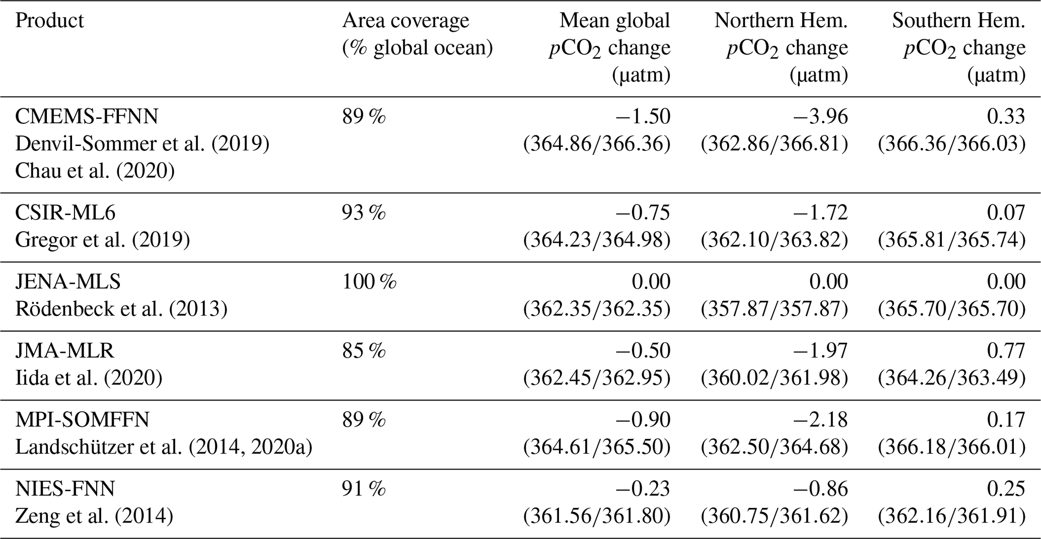
All of these methods provide three-dimensional fields (latitude, longitude, time) of the sea surface pCO2 and the air–sea CO2 flux. In their original form, each product may utilize different choices for the inputs to Eq. (1) (Table A1). While the choices made by each product's creator, listed in Table A1, are not incorrect, by utilizing a uniform methodology in flux calculation, provided by pySeaFlux, the differences in the resulting flux estimate can be attributed to the pCO2 mapping method itself. In this work we recompute the fluxes using the following inputs to the bulk parameterization approach Eq. (1): kw is the gas transfer velocity (further discussed in Sect. 2.3); sol is the solubility of CO2 in seawater (in units of mol m−3 µatm−1), calculated using the formulation by Weiss (1974), near-surface EN4 salinity (Good et al., 2013), NOAA Optimum Interpolation Sea Surface Temperature V2 (OISSTv2) (Reynolds et al., 2002), and European Centre for Medium-Range Weather Forecasts (ECMWF) ERA5 sea level pressure (Hersbach et al., 2020); ice is the sea-ice fraction from NOAA OISSTv2 (Reynolds et al., 2002); pCO2 is the partial pressure of oceanic CO2 (in µatm) for each observation-based product after filling, as discussed in Sect. 2.1; and pCO is the dry air mixing ratio of atmospheric CO2 (xCO2) from the ESRL surface marine boundary layer CO2 product available at https://www.esrl.noaa.gov/gmd/ccgg/mbl/data.php (last access: 10 October 2020) (Dlugokencky et al., 2019) multiplied by ERA5 sea level pressure (Hersbach et al., 2020) at monthly resolution and applying the water vapor correction according to Dickson et al. (2007). All of the components of Eq. (1) are available in the SeaFlux dataset.
Throughout this study, flux is defined as being positive when CO2 is released from the ocean to the atmosphere and negative when CO2 is absorbed by the ocean from the atmosphere. In the following sections, we discuss the three steps that have the greatest impact on the inconsistencies between flux calculations in the six pCO2 products and the approach that we utilize for the SeaFlux ensemble product.
2.1 Step 1: area filling
Machine learning methods aim to maximize the utility of the existing in situ observations by extrapolation using various proxy variables for processes influencing changes in ocean pCO2. Extrapolation with these independently observed variables is possible due to the nonlinear relationship between pCO2 in the surface ocean and the proxies that drive these changes. However, not all of the proxy variables have complete global ocean coverage for all months; therefore, the resulting pCO2 products are limited by the extent of the proxy variables (Figs. 1, A1). Additionally, in continental shelf regions, there is the potential that different relationships of pCO2 to the proxy variables are expected as opposed to in the open ocean, thus limiting the extrapolations. The mixed layer scheme (utilized by the JENA-MLS product) does not suffer from such missing areas but also does not distinguish between coastal and open ocean; it is stated to be an open ocean product which is extrapolated to the full global coverage (Rödenbeck et al., 2013). For this reason, it is not utilized in SeaFlux as a potential product for filling missing areas in the other pCO2 products.

Figure 1Maps showing the fraction of months (1990–2019) with coverage available for each of the six pCO2 data products used in this study. Blue regions represent full temporal coverage of pCO2 in the product, while yellow areas show regions with no reported pCO2 values for any month of the time series.
To account for differing area coverage, past studies (Friedlingstein et al., 2019, 2020; Hauck et al., 2020) have adjusted observation-based flux products by simply scaling their global flux based on the percent of the total ocean area represented (Fig. A2). This does not account for the fact that some areas have CO2 flux densities that are higher or lower than the global average, and their adjustment would be based on that mean value (Tables 1, 3). Thus, the magnitude of the adjustment by area-scaling is likely an underestimate in some years or products (McKinley et al., 2020). One specific example is the northern high latitudes where coverage by the six products varies substantially. Similarly, three products provide estimates in marginal seas such as the Mediterranean, while the other three products have no reported pCO2 values here.
To address the inconsistent spatial coverage in products we utilize a newly released open and coastal merged climatology product (MPI-ULB-SOMFFN; Landschützer et al., 2020b, c) that is a blend of the coastal ocean SOMFFN mapping method (Laruelle et al., 2017) and the open ocean equivalent (MPI-SOMFFN; Landschützer et al., 2020a). The merged product includes full coverage of open ocean pCO2 along with coastal ocean regions, marginal seas, and the Arctic Ocean at 1∘ by 1∘ or finer spatial resolution. A potential alternative resource for filling the missing regions is the OceanSODA-ETHZ surface pCO2 product (Gregor and Gruber, 2021) that maps both the open ocean and marginal seas explicitly for the period 1985–2018 (unlike the JENA-MLS approach). However, as with other products, OceanSODA-ETHZ has limited coverage in the Arctic. A comparison of the overlapping regions between the MPI-ULB-SOMFFN and OceanSODA-ETHZ products shows good agreement (Fig. A3). We have confidence moving forward using solely MPI-ULB-SOMFFN for area-filling, as including OceanSODA-ETHZ would not result in substantially different results and would be constrained by its limited Arctic coverage.
For each observation-based product, we fill missing grid cells with a scaled value based on the global-coverage MPI-ULB-SOMFFN climatology (Fig. 2). The scaling accounts for year-to-year changes in pCO2 in the missing areas (given that the extended MPI-ULB-SOMFFN product is a monthly climatology centered on the year 2006) and is obtained as follows.

Figure 2Maps demonstrating the filling procedure employed in this study using a snapshot of pCO2 from May 2013. (a) Map of unfilled CSIR-ML6 pCO2. (b) The scaled pCO2 climatology of Landschützer et al. (2020b). (c) The mean pCO2 for the scaled climatology over time. (d) The CSIR-ML6 pCO2 product (a) filled using the scaled climatology (b).
To extend the open and coastal merged climatology (MPI-ULB-SOMFFN) to 1990–2019, we calculate a global scaling factor based on the product-based ensemble mean pCO2 for regions that are covered consistently by all six pCO2 products. We first mask all pCO2 products to a common sea mask before taking an ensemble mean (pCO). Next, we divide this ensemble mean by the MPI-ULB-SOMFFN climatology (pCO) at monthly 1∘ by 1∘ resolution (Eq. 2). The monthly scaling factor (sf) is calculated by taking the mean over the spatial dimensions. An alternative method of calculating the scaling factor individually for each pCO2 product yields very similar results; the benefit of the ensemble approach is that it allows for the scaling factor to be quickly utilized for any other pCO2 product under development.
The scaling factor calculation can be represented as
where sf is the one-dimensional scaling factor (time dimension), pCO is the ensemble mean of all pCO2 products at three dimensions, monthly 1∘ by 1∘ resolution, pCO is the MPI-ULB-SOMFFN climatology, also at three dimensions but limited to just one climatological year. The x and y indicate that we take the area-weighted average over longitude (x) and latitude (y) resulting in the monthly one-dimensional scaling value. If a product mean is exactly equal to the climatology mean, the scaling factor is 1. The value ranges from 0.91 to 1.06 over the 30-year period. The one-dimensional scaling factor is then multiplied by the MPI-ULB-SOMFFN climatology for each spatial point resulting in a three-dimensional scaled filling map. These values are then used to fill in missing grid cells in each observation-based product.
Globally, the area-filling adjustments result in a difference of less than 17 % of the total flux in all products, with the mean adjustment for the six products at 8 %. In the Northern Hemisphere, however, the filling process can drive adjustments of up to 32 % due to missing coverage in the North Atlantic specifically (Fig. 1, Table 3). As expected, the observation-based products with more complete spatial coverage tend to have smaller flux adjustments. However, the impact on the final CO2 flux depends on both the ΔpCO2 and wind speed of the areas being filled (Figs. 2–3, Tables 1, 3). The only product that does not change during this adjustment process is the JENA-MLS mixed-layer scheme-based product (Rödenbeck et al., 2013) which is produced with full spatial coverage and therefore needs no spatial filling; any difference between filled/unfilled for this product is due to the ocean mask applied in SeaFlux.
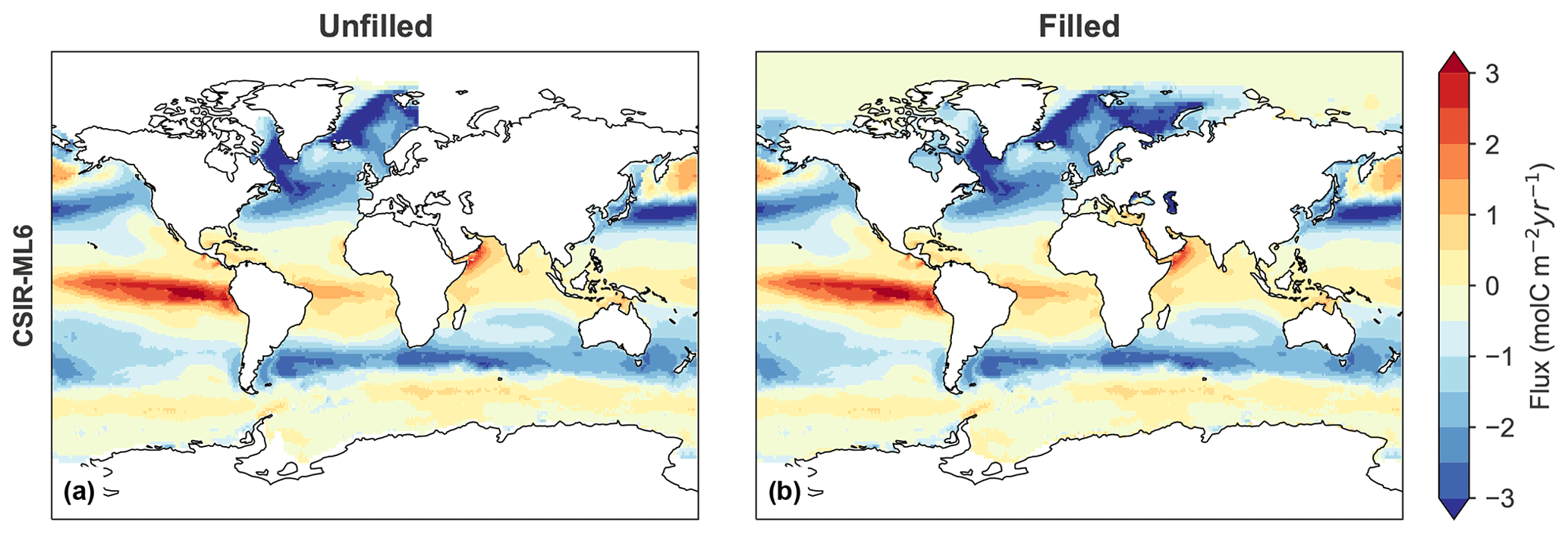
Figure 3Mean flux (mol m−2 yr−1) for 1990–2019 for CSIR-ML6 product. (a) Map of mean-calculated flux using the original pCO2 product and three scaled wind products (CCMPv2, ERA5, JRA55); (b) map of mean-calculated flux using the filled pCO2 product and three scaled wind products. Similar maps for all other products are available in Fig. A5.
Our approach is not without its own assumptions and limitations. We rely on a single estimate to fill the missing pCO2 given that this is the only publicly available coastal-resolution product currently existing. Nevertheless, the fact that common missing areas along coastal regions and marginal seas are reconstructed using specific coastal observations provides a step forward from the linear-scaling approach currently used by the Global Carbon Budget (Friedlingstein et al., 2019, and Fig. A2 in Friedlingstein et al., 2020). Further confidence is provided by previous research showing that climatologically relevant signals, i.e., mean state and seasonality, are well reconstructed by the MPI-SOMFFN method (Gloege et al., 2021).
Furthermore, our scaled filling methodology assumes that pCO2 in the missing ocean regions is increasing at the same rate as the common area of open ocean pCO2 used to calculate the scaling factor. Research from coastal ocean regions and shelf seas reveal that, in spite of a large spatial heterogeneity, this is a reasonable first-order approximation (Laruelle et al., 2018).
Any method of artificially filling in missing areas introduces additional uncertainty to the flux estimates. However, this introduced uncertainty is necessary for true global intercomparison efforts. A concern is that the filling method would artificially lower the spread of the products in the SeaFlux ensemble. We do not find this to be the case. The standard deviation of the mean flux for a most conservative mask, which includes only those grid cells with values reported for all six pCO2 products for all months, is nearly identical to the standard deviation of the final version of the SeaFlux product ensemble. This comparison indicates that our filling method does not in fact artificially lower the uncertainty or decrease the spread of the products.
2.2 Step 2: wind product selection
Historical wind speed observations (including measurements from satellites and moored buoys) are aggregated and extrapolated through modeling and data assimilation systems to create global wind reanalyses. These reanalyses are required to compute air–sea gas exchange. Air–sea flux is commonly parameterized as a function of the gradient of CO2 between the ocean and the atmosphere with wind speed modulating the rate of the gas exchange (Eq. 1). Each of these wind reanalyses has strengths and weaknesses, specifically on regional and seasonal scales (Chaudhuri et al., 2014; Roobaert et al., 2018; Ramon et al., 2019), but all are considered reasonable options by the community (Roobaert et al., 2018). The pySeaFlux package includes options for the user to select their wind product of choice. For the SeaFlux ensemble product, we use three wind reanalysis products for completeness: the Cross-Calibrated Multi-Platform v2 (CCMP2; Atlas et al., 2011), the Japanese 55-year Reanalysis (JRA-55; Kobayashi et al., 2015), and the European Centre for Medium-Range Weather Forecasts (ECMWF) ERA5 (Hersbach et al., 2020). The wind speed (U10) is calculated at the native resolution of each wind product from u and v components of wind. Details of each wind product are shown in Table A2.
2.3 Step 3: calculation of gas transfer
We employ the quadratic wind speed dependence (Wanninkhof, 1992; Ho et al., 2006) and calculate the gas transfer velocity (kw) for each of the wind reanalysis products as
where the units of kw are in centimeters per hour (cm h−1), Sc is the dimensionless Schmidt number, and 〈U2〉 denotes the square of average 10 m high winds (m s−1), also referred to as the second moment of the wind speed. We choose the quadratic dependence of the gas transfer velocity as it is widely accepted and used in the literature (Wanninkhof, 1992; Ho et al., 2006); however, we acknowledge that the actual relationship could vary from less than linear (Krakauer et al., 2006) to cubic (Wanninkhof and McGillis, 1999; Stanley et al., 2009). Observational and modeling studies have often suggested that different parameterizations could be more appropriate under specific conditions such as in regions of high wind speeds (Fairall et al., 2000; Nightingale et al., 2000; McGillis et al., 2001; Krakauer et al., 2006); recent direct carbon dioxide flux measurements made in the high-latitude Southern Ocean confirm that even in this high wind environment, a quadratic parameterization fits the observations best (Butterworth and Miller, 2016). Future updates of SeaFlux will include kw for other parameterizations (e.g., cubic).
We calculate the square of the wind speed at the native resolution of each wind product and then average it to 1∘ by 1∘ monthly resolution (see Table A2). The order of this calculation is important as variability is lost when resampling data to lower resolutions because of the concavity of the quadratic function. For example, taking the square of time-averaged wind speeds would result in an underestimate of the gas transfer velocity (Sarmiento and Gruber, 2006; Sweeney et al., 2007). The resulting second moment is equivalent to , where Umean and Ustd are the temporal mean and standard deviation calculated from the native temporal resolution of U.
In addition to the choice of wind parameterization (Roobaert et al., 2018), large differences in flux can result due to the scaling of the coefficient of gas transfer (a) applied when calculating the global mean gas transfer velocity. This constant originates from the gas exchange process studies (Krakauer et al., 2006; Sweeney et al., 2007; Müller et al., 2008; Naegler, 2009) which utilize observations of radiocarbon data from the GEOSECS and WOCE/JGOFS expeditions (Key et al., 2004). The 14C released from nuclear bomb testing (hence bomb-14C) in the mid-20th century has since been taken up by the ocean. The number of bomb-14C atoms in the ocean, relative to the pre-bomb 14C, can thus be used as a constraint on the long-term rate of exchange of carbon between the atmosphere and the ocean. This coefficient, a, is not consistent for each wind product and must thus be individually calculated via the equation based on equation 39 from Naegler (2009):
the parameters of which are defined in Eq. (3). The units of the coefficient a are (cm h−1) (m s−1)−2. In the cost function, a global average of kw is set for which several estimates exist in the literature (ranging from 15.1 to 18.2 cm h−1), introducing another source of uncertainty as shown in Table A1 (Krakauer et al., 2006; Naegler et al., 2006; Sweeney et al., 2007; summarized in Table 2 of Naegler, 2009). Naegler (2009) show that these estimates fall within the ∼20 % range of uncertainty of the bomb-14C-constrained global average kw, which they estimate at 16.5 ± 3.2 cm h−1. We scale kw to this single value (16.5 cm h−1) over the three-decade period 1990–2019.
Our scaled coefficients (Table 2) correspond well with the estimate of Wanninkhof (2014) who uses the CCMP wind product to estimate a as 0.251, whereas our estimate of a for CCMP is 0.257. Scaling kw to a single global value (here, 16.5 cm h−1) for all wind products reduces the spread of flux estimates, but it does not reduce the uncertainty which remains ∼20 %. This uncertainty must be accounted for when reporting fluxes (Naegler, 2009; Wanninkhof, 2014). In this work, we refer to this uncertainty, which is inherent to the formulation and scaling of kw, as intrinsic uncertainty, which we do not try to reduce with SeaFlux and include in our reported uncertainty estimate. However, by correctly scaling kw for each wind product we reduce the disharmony associated with incorrect scaling by up to 9 %, depending on which pCO2 and wind reanalysis products are considered. This is consistent with previous results shown by Roobaert et al. (2018, 2019).
Table 2CSIR-ML6 product flux values. Column 1 lists the scaled coefficient of gas transfer for each of the three wind reanalysis products. Column 2 includes the global mean flux using each wind product. Column 3 shows the difference in resulting flux when using a scaled coefficient of gas transfer versus a set value of 0.26. All flux values reported are from the area-filled product version. All values are computed over the period 1990–2019.
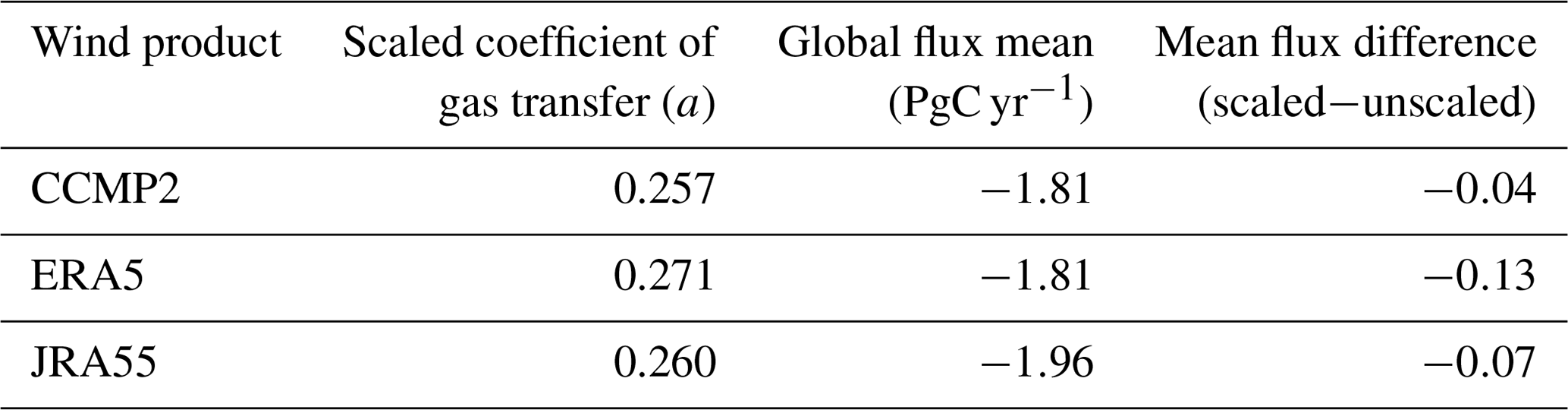
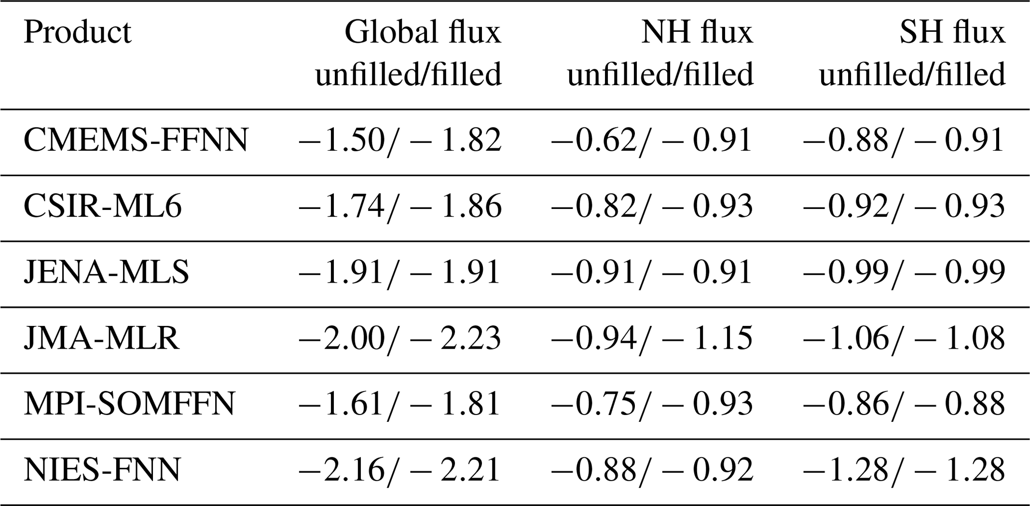
Table 3Mean air–sea fluxes (PgC yr−1) for 1990–2019 using the mean of three wind products, calculated for the filled global area and the unfilled native “global” area for each pCO2 product. The Northern Hemisphere (NH) and Southern Hemisphere (SH) fluxes (unfilled/filled) are included to highlight the imbalanced regional effect of the spatial filling process.
2.4 Further parameters for flux calculation
The remaining parameters of Eq. (1) are the solubility of CO2 in seawater (sol), the atmospheric partial pressure of CO2 (pCO), and the area weighting to account for sea-ice cover. While the choices of products used for these parameters can also result in differences in flux estimates, the impacts are much smaller as compared with the parameters discussed above.
Atmospheric pCO2 is calculated as the product of surface xCO2 and sea level pressure corrected for the contribution of water vapor pressure. The choice of the sea level pressure product or absence of the water vapor correction can have a small, but not insignificant, impact on the calculated fluxes. Additionally, some products utilize the output of an atmospheric CO2 inversion product (e.g., CarboScope, Rödenbeck et al., 2013; CAMS CO2 inversion, Chevallier, 2013) which can introduce differences in the flux estimate outside of the sources related to a product's surface ocean pCO2 mapping method. Importantly, we do not advocate that our estimate of pCO is an improvement over other estimates thereof; rather we provide an estimate of pCO that has few assumptions and leads to a methodologically consistent estimate of ΔpCO2. We maintain the same philosophy in our estimates of the solubility of CO2 in seawater and sea-ice area weighting, and therefore we do not elaborate on them here.
3.1 SeaFlux air–sea CO2 flux calculation
Following Eq. (1), CO2 flux is calculated individually for each of the six observation-based products with three available wind products (CCMPv2, ERA5, JRA55), as discussed in Sect. 2.2 (Table 4). Since we account for spatial coverage differences via our filling method (Sect. 2.1), taking a global mean flux for each of the data products truly follows the definition of “global” for each original product. Figure 4 shows the difference these wind products generate on the resulting global mean flux of the CSIR-ML6 product as one example (other products in Fig. A4). The three wind products show consistent fluxes throughout the time series, with the importance of appropriate scaling of the coefficient of gas transfer (a) evident in the significant differences between global mean fluxes calculated with unscaled and scaled a values (Fig. 4, Table 2). It is clear that the impact of applying the appropriate coefficient of gas transfer through proper scaling has an impact on the resulting flux time series.
Table 4Mean fluxes (PgC yr−1) for each observational pCO2 product over the period 1990–2019. Mean flux is calculated from filled coverage pCO2 map and scaled gas exchange coefficient; global mean flux is for three wind products (CCMP2, ERA5, JRA55) and the average. The time series of the mean flux values for each product (rightmost column) are plotted in Fig. 5.
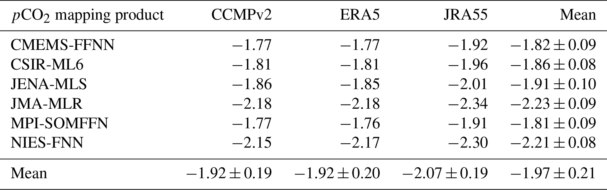
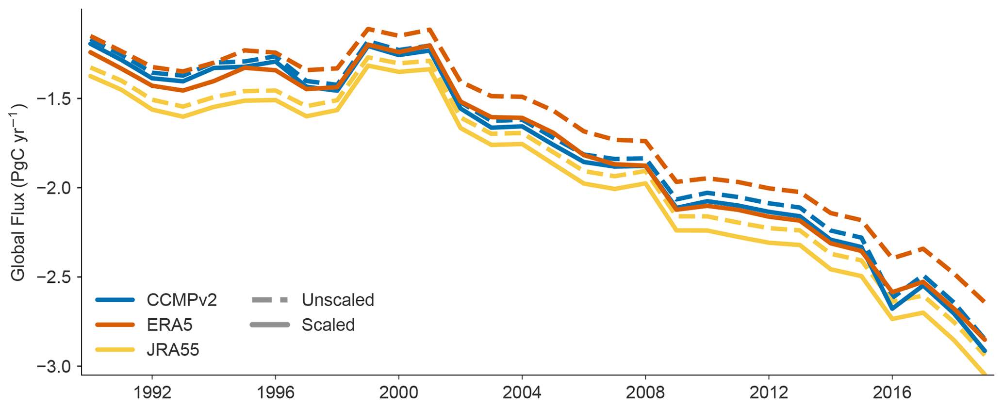
Figure 4CSIR-ML6-calculated air–sea CO2 flux time series for various wind speed products, scaled (solid) and unscaled (dashed; a=0.251). Time series plots for all pCO2 products and including two additional wind products (NCEP1 and NCEP2) are included in Fig. A4.
3.2 SeaFlux ensemble flux
By calculating each product's air–sea CO2 flux using consistent inputs described in Sect. 3.1, a more accurate comparison of fluxes with the SeaFlux ensemble is permitted. Combining all fluxes, we derive a mean flux estimate of −1.97 ± 0.45 PgC yr−1 (Tables 4, A3). We discuss the calculation of the uncertainty in the following section. This flux estimate is strengthened by the use of multiple observation-based pCO2 products and wind products which we consider to be independent estimates for the purpose of the uncertainty calculation. These flux values are different from those produced by the observation-based pCO2 product's original creator, both spatially and on the mean (Figs. 5, A5, Tables A1, A3). However, by calculating fluxes in such a consistent manner, we on the one hand gain more confidence in the ensemble mean estimate as it considers representations using a variety of pCO2 reconstructions, gas transfer parametrizations, and wind products, and on the other hand, we have a more realistic uncertainty representation than previous estimates based on a single pCO2 reconstruction.
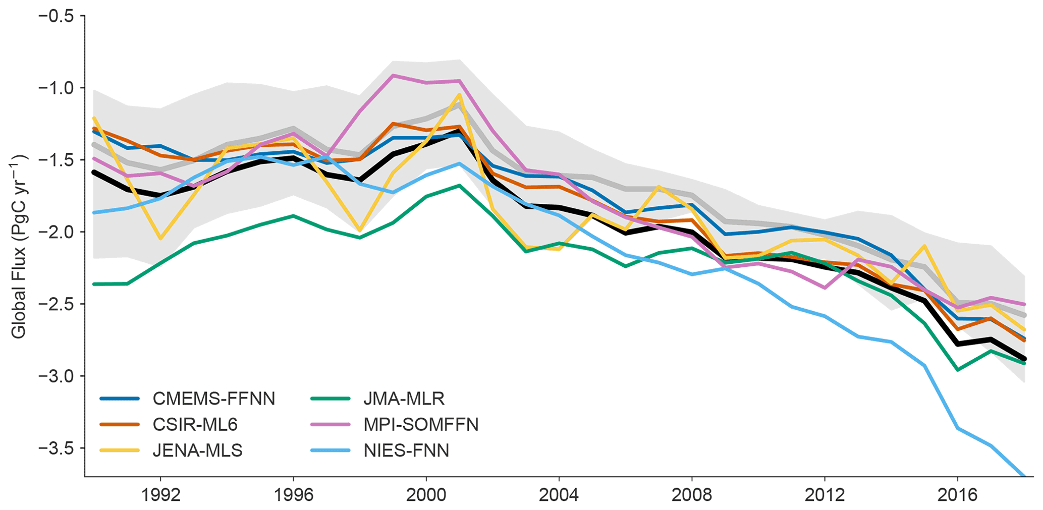
Figure 5Global flux time series from six observation-based products. Color lines show fluxes calculated from the standardized approach presented here (spatial filling with flux is calculated from three wind products, and the average flux is then plotted here); the black line shows the mean of six products. The shaded region shows the spread of original flux calculations from product creators with the mean in gray.
3.3 Uncertainty discussion
All flux estimates using such parameterizations are not without significant uncertainties, and SeaFlux is no exception. We estimate the uncertainty of the flux estimate to be 0.45 PgC yr−1. Here, the stated spread represents , where (0.19 PgC yr−1) is the mean standard deviation over the six filled pCO2 products, σwind (0.09 PgC yr−1) is the mean standard deviation over the three wind products included in the SeaFlux product, and (0.39 PgC yr−1) is the 20 % uncertainty in the gas transfer velocity and associated scaling flux parameterization (Wanninkhof, 2014). This last estimate shows that there is significant intrinsic uncertainty inherent to the method of calculation, as estimated by Naegler (2009) and Wanninkhof (2014).
Currently, there is only one product available designed to estimate the pCO2 of coastal oceans, the Arctic Ocean, and marginal seas, and this has the potential to cause an underestimation of . It would be beneficial to likewise have an ensemble of estimates in these regions to better constrain the uncertainty attached to this filling approach. Therefore, while our current analysis shows that the chosen filling method does not itself reduce the spread in the products, we push the community to extend their products to the coastal ocean so as to eliminate the need for this correction in the future.
While the SeaFlux product is unable to further reduce these sources of uncertainty, the strength of the product is that it provides an estimated flux with no source of difference that is not implicit in the mapping method or flux calculation.
3.4 Issues not addressed by SeaFlux
While SeaFlux presents one approach to standardize the calculation of air–sea carbon flux, there remain issues that the ocean carbon community is still working towards understanding and incorporating. One such issue has been raised by Watson et al. (2020) who contend that a correction should be applied to in situ pCO2 observations to account for the vertical temperature gradient between the ship water intake depth and the surface skin layer where gas exchange actually takes place. A further correction should be applied when calculating fluxes to account for the “cool skin” effect caused by evaporation (Woolf et al., 2016; Watson et al., 2020). Applying these corrections results in an increasing CO2 sink by up to 0.9 PgC yr−1 (Watson et al., 2020). Here, we do not take such adjustments into account for two reasons. Firstly, the skin temperature correction to pCO2 needs to be applied directly to the measurements and not the final interpolated pCO2 from the data products. Hence, it is up to the developers of the SOCAT dataset and the developers of the pCO2 mapping products to decide on the inclusion of this correction. It would then be up to the developers of the data products to update their mapped products. Secondly, the cool skin correction would be equally applied to all methods and would not contribute to the inconsistencies in flux calculation that we are trying to address here. As the ocean carbon community moves towards consensus on such issues, SeaFlux will be updated to include revised protocols.
To compare these estimates of contemporary air–sea net flux (Fnet) from surface ocean pCO2 with estimates of the anthropogenic carbon flux from interior data (Mikaloff Fletcher et al., 2006; DeVries, 2014; Gruber et al., 2019) or from global ocean biogeochemical models (Friedlingstein et al., 2020; Hauck et al., 2020), it is necessary to account for the outgassing of natural carbon, which was supplied to the ocean by rivers, as well as the non-steady-state behavior of the natural carbon cycle (Hauck et al., 2020). Work is ongoing to quantify the lateral river carbon flux transported into the coastal and open oceans. Current estimates are 0.23 PgC yr−1 (Lacroix et al., 2020), 0.45 PgC yr−1 (Jacobson et al., 2007), and 0.78 PgC yr−1 (Resplandy et al., 2018), and the regional distribution of the resulting outgassing remains understood only from a few model simulations (Aumont et al., 2001; Lacroix et al., 2020). In addition, quantification of non-steady-state behavior of the natural carbon cycle has only recently been proposed, and significant uncertainty remains, with a magnitude range of 0.05–0.4 PgC yr−1 for 1994–2007 (Gruber et al., 2019; McKinley et al., 2020). Similar to the cool skin correction suggested by Watson et al. (2020) discussed above, in this work we have not included these adjustments here as they would not contribute to the inconsistencies between the different products for Fnet itself, which is our focus.
Data (Gregor and Fay, 2021) are available on Zenodo (https://doi.org/10.5281/zenodo.5482547), and the software used to generate these data is available on GitHub (https://github.com/lukegre/pySeaFlux, last access: 9 September 2021). NOAA_OI_SST_V2 data are provided by the NOAA/OAR/ESRL PSL, Boulder, Colorado, USA (Reynolds et al., 2002, https://doi.org/10.1175/1520-0442(2002)015<1609:AIISAS>2.0.CO;2).
We introduce SeaFlux, a dataset that facilitates a standardized approach for flux calculations from observation-based pCO2 products. Specifically, we address the two largest sources of divergence in air–sea flux calculation, namely the differences in spatial coverage between the products and the scaling of the gas transfer velocity for available wind speed products based on global 14C-based constraints. The area adjustment is the largest contributor to the methodological discrepancies, resulting in an increase in CO2 uptake of 0 %–17 % relative to the original, possibly incomplete coverage (depending on pCO2 product). The global scaling of the gas transfer velocity can change the CO2 flux on average by 5 % relative to non-standardized flux calculations. The impact of applying the appropriate gas exchange coefficient through proper scaling has a larger impact on the resulting flux time series than solely the choice of wind product. By accounting for these sources of differences, the global mean-calculated air–sea carbon flux calculated from the six available products is adjusted by up to 21 %. The SeaFlux ensemble mean air–sea carbon flux is estimated to be −1.97 ± 0.45 PgC yr−1 with the spread representing 1σ as calculated from the 18 realizations.
This work provides an ensemble data product of the air–sea CO2 flux predicated on observation-based pCO2 products. This ensemble product is meant to facilitate the use of the pCO2 observation-based ocean flux estimates in assessment studies of the global carbon cycle, such as the Global Carbon Budget or RECCAP-2. Note that the original pCO2 products still offer additional information important in other applications, such as coverage over longer time periods, higher spatial or temporal resolution, or runs incorporating further auxiliary datasets or pCO2 data (e.g., SOCCOM float data; Bushinsky et al., 2019).
Along with the ensemble of CO2 flux fields, we also provide a public-use coding package (pySeaFlux) allowing users to apply the presented standardized flux calculations to their own data-based pCO2 reconstructions.
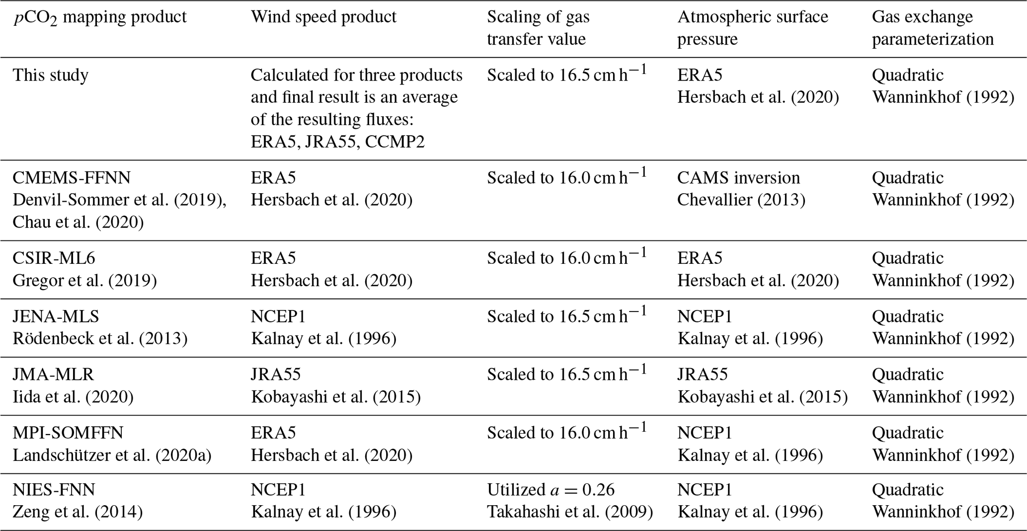
Table A2Summary of wind products used in this study. Note that the date range starts for the first full year of data. We do not use NCEP1/2 in our main results, but these are included for reference. Time units are in hours and space in degrees. Mean wind speed is given for the ice-free ocean for the three-decade period 1990–2019.
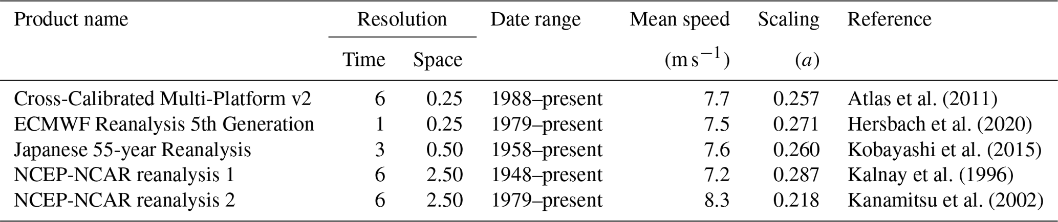
Table A3Mean fluxes (PgC yr−1) for 1990–2019 for each observational pCO2 product. Mean flux calculated from unfilled (filled) coverage pCO2 map and unscaled/scaled coefficient of gas transfer (unscaled = 0.251), calculated for three wind products (CCMP2, ERA5, JRA55) with the average shown here. Percent change is calculated as the difference between the unfilled–unscaled and filled–scaled as a fraction of the filled–scaled; it does not indicate an error in the product's flux but is a representation of the impact the filling and scaling can have on the end flux estimate. The mean flux as reported in the original pCO2 product is included for comparison (Fig. 5).
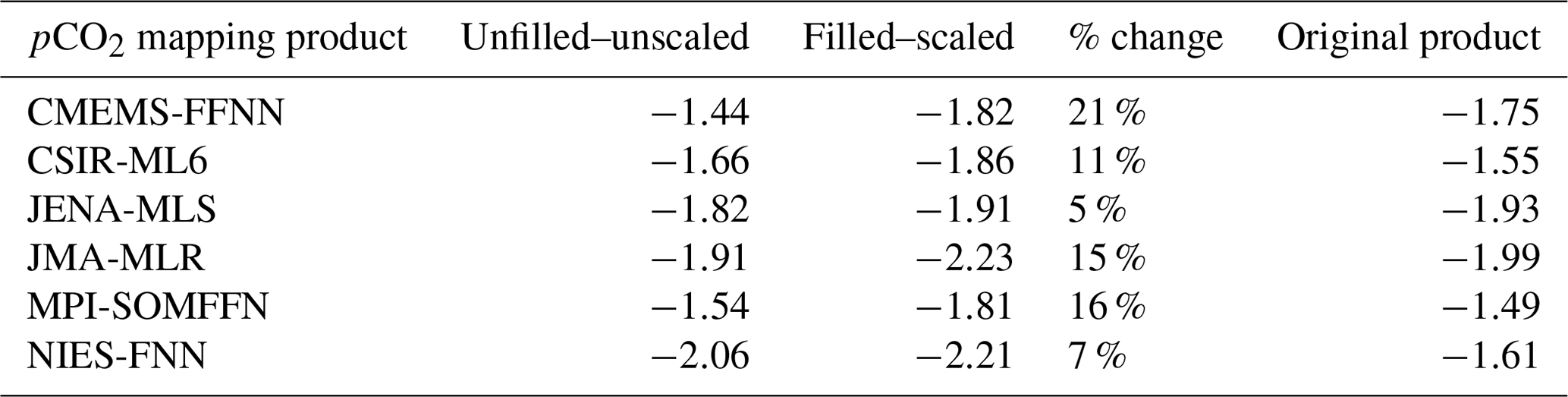
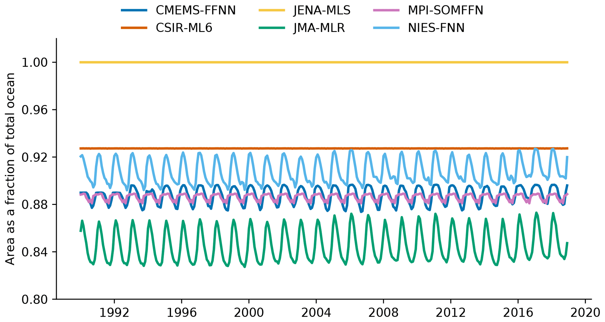
Figure A1Time series showing the fraction of area covered by observations as a function of time (monthly) for the six pCO2 data products used in this study.

Figure A2Annual time series of the additional flux amount calculated by the area-weighted method used in the Global Carbon Budget (a) and a similar plot showing the annual additional flux using the SeaFlux methodology (b).
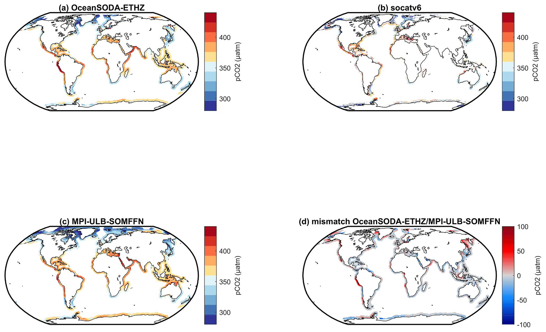
Figure A3Spatial distributions of the annual mean pCO2 (µatm) generated by (a) ETHZ-OceanSODA, (b) extracted from the SOCATv6 database, and (c) from the MPI-ULB merged product. (d) Bias between panels (a) and (c) (in µatm; red colors correspond to regions in which the pCO2 from ETHZ-OceanSODA is higher than the MPI-ULB merged product). There is good agreement between the products on a regional scale.
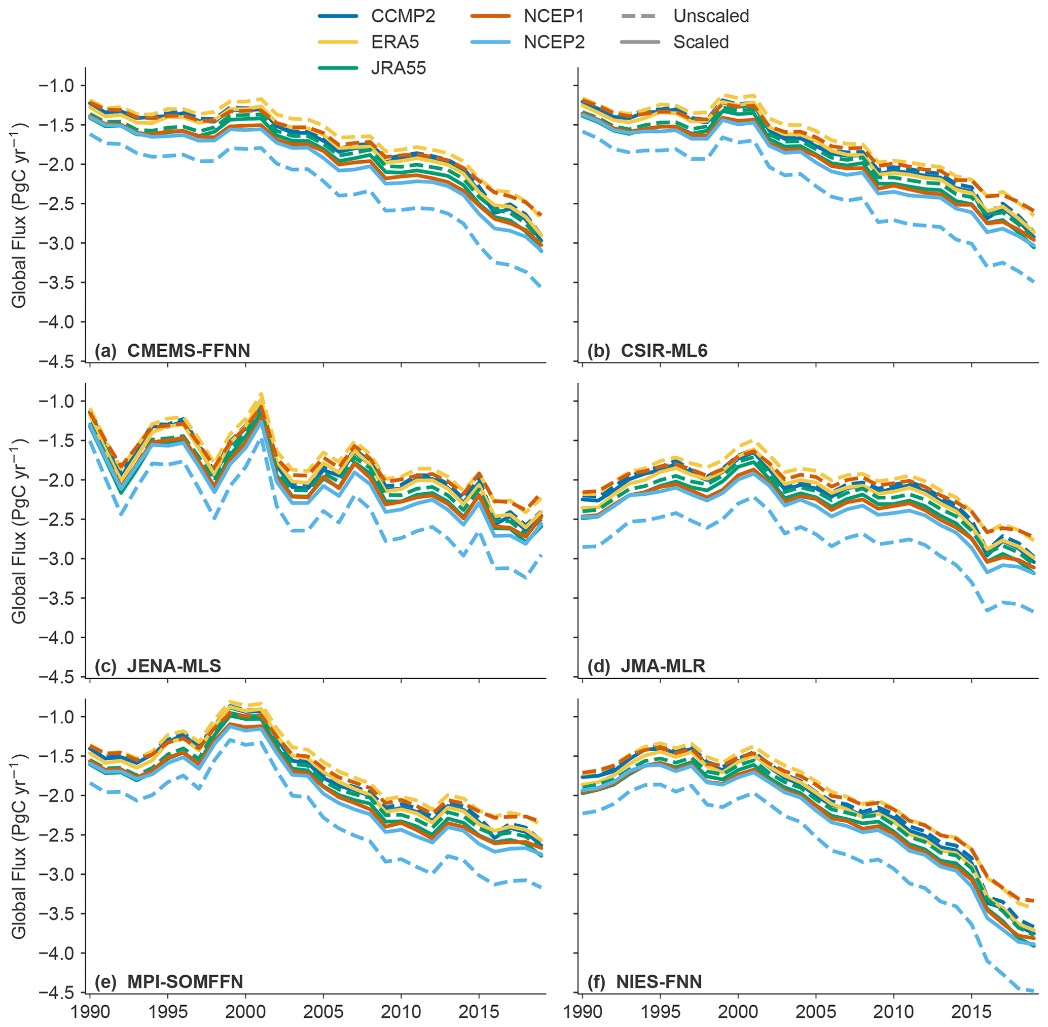
Figure A4Air–sea CO2 flux time series (PgC yr−1) calculated using five wind speed products (CCMPv2, ERA5, JRA55, NCEP1, NCEP2), scaled (solid) and unscaled (dashed).
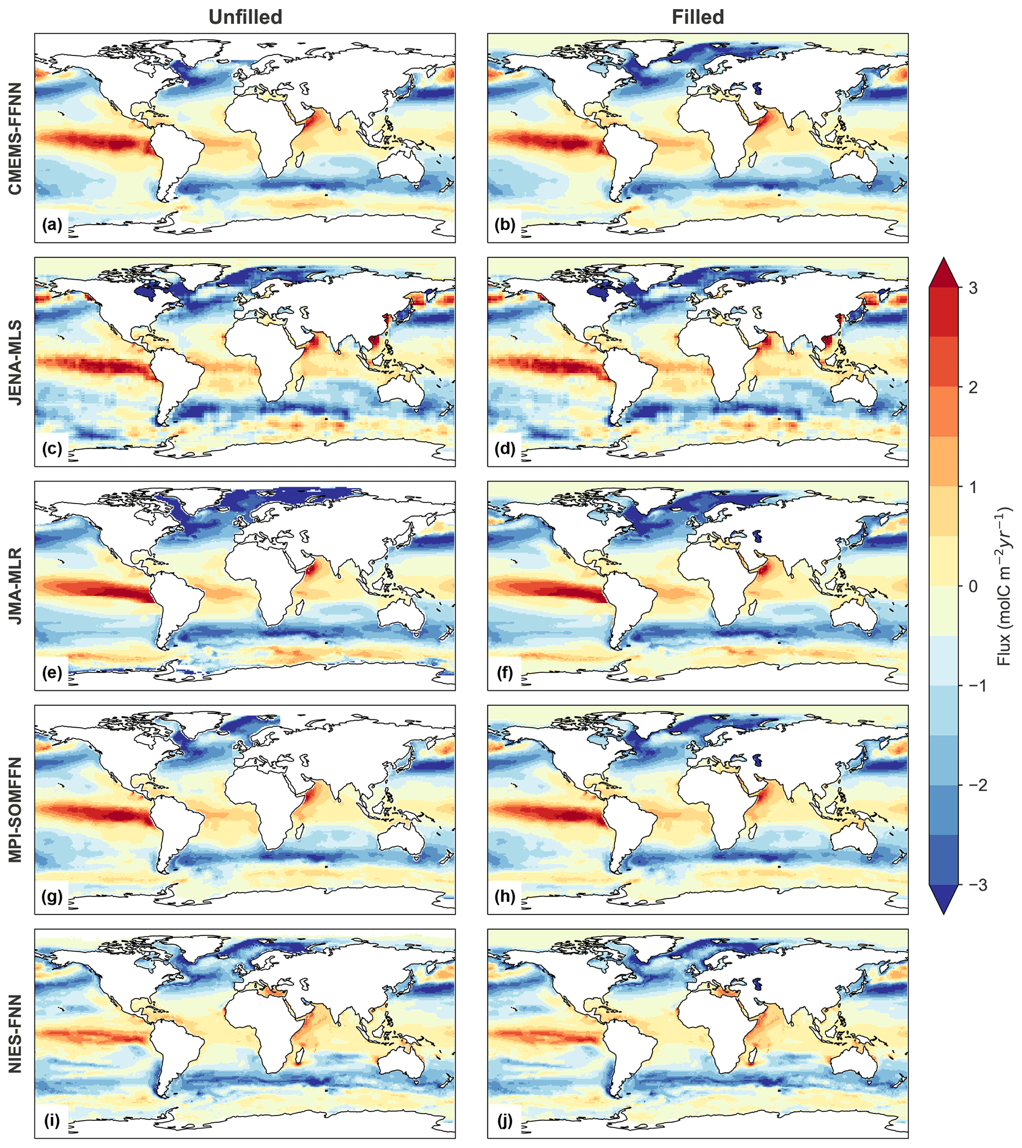
Figure A5Mean flux (mol m−2 yr−1) for 1990–2019. Left-hand column: map of mean-calculated flux using the unfilled pCO2 product and three scaled wind products. Right-hand column: map of mean-calculated flux using the filled pCO2 product and three scaled wind products.
ARF and LG designed the experiment, and LG developed the model code and performed the simulations with ARF focusing on analysis. ARF and LG collectively prepared the manuscript with contributions from all co-authors. LG, PL, MG, YI, GGL, CR, and JZ contributed data products to the ensemble. GAM, NG, AR, PL, MG, GGL, and CR contributed to the development of the manuscript through comments and discussions.
The authors declare that they have no conflict of interest.
Publisher’s note: Copernicus Publications remains neutral with regard to jurisdictional claims in published maps and institutional affiliations.
Peter Landschützer, Nicolas Gruber, and Luke Gregor acknowledge the funding support from the European Community. Galen A. McKinley and Amanda R. Fay acknowledge the funding from Columbia University and the National Science Foundation; Galen A. McKinley was also supported by the National Oceanic and Atmospheric Administration. The Surface Ocean CO2 Atlas (SOCAT) is an international effort, endorsed by the International Ocean Carbon Coordination Project (IOCCP), the Surface Ocean Lower Atmosphere Study (SOLAS), and the Integrated Marine Biosphere Research (IMBeR) program, to deliver a uniformly quality-controlled surface ocean CO2 database. The many researchers and funding agencies responsible for the collection of data and quality control are thanked for their contributions to SOCAT. Goulven G. Laruelle is research associate of the F.R.S-FNRS at the Université Libre de Bruxelles.
Peter Landschützer, Nicolas Gruber, and Luke Gregor received funding from the European Community's Horizon 2020 Project under grant agreement no. 821003 (4C). Galen A. McKinley and Amanda R. Fay received funding from Columbia University and the National Science Foundation (grant no. OCE1948624). Galen A. McKinley is also supported by the National Oceanic and Atmospheric Administration (agreement no. NA20OAR4310340). Marion Gehlen received funding from the European Copernicus Marine Environment Monitoring Service (CMEMS) under grant no. 83-CMEMS-TAC-MOB.
This paper was edited by David Carlson and reviewed by Timothy DeVries, Andrea Fassbender, and Rik Wanninkhof.
Atlas, R., Hoffman, R. N., Ardizzone, J., Leidner, S. M., Jusem, J.C., Smith, D. K., and Gombos, D.: A cross-calibrated, multiplatform ocean surface wind velocity product for meteorological and oceanographic applications, B. Am. Meteorol. Soc., 92, 157–174, https://doi.org/10.1175/2010BAMS2946.1, 2011.
Aumont, O., Orr, J. C., Monfray, P., Ludwig, W., Amiotte-Suchet, P., and Probst, J.-L.: Riverine-driven interhemispheric transport of carbon, Global Biogeochem. Cy., 15, 393–405, https://doi.org/10.1029/1999GB001238, 2001.
Bakker, D. C. E., Pfeil, B., Landa, C. S., Metzl, N., O'Brien, K. M., Olsen, A., Smith, K., Cosca, C., Harasawa, S., Jones, S. D., Nakaoka, S., Nojiri, Y., Schuster, U., Steinhoff, T., Sweeney, C., Takahashi, T., Tilbrook, B., Wada, C., Wanninkhof, R., Alin, S. R., Balestrini, C. F., Barbero, L., Bates, N. R., Bianchi, A. A., Bonou, F., Boutin, J., Bozec, Y., Burger, E. F., Cai, W.-J., Castle, R. D., Chen, L., Chierici, M., Currie, K., Evans, W., Featherstone, C., Feely, R. A., Fransson, A., Goyet, C., Greenwood, N., Gregor, L., Hankin, S., Hardman-Mountford, N. J., Harlay, J., Hauck, J., Hoppema, M., Humphreys, M. P., Hunt, C. W., Huss, B., Ibánhez, J. S. P., Johannessen, T., Keeling, R., Kitidis, V., Körtzinger, A., Kozyr, A., Krasakopoulou, E., Kuwata, A., Landschützer, P., Lauvset, S. K., Lefèvre, N., Lo Monaco, C., Manke, A., Mathis, J. T., Merlivat, L., Millero, F. J., Monteiro, P. M. S., Munro, D. R., Murata, A., Newberger, T., Omar, A. M., Ono, T., Paterson, K., Pearce, D., Pierrot, D., Robbins, L. L., Saito, S., Salisbury, J., Schlitzer, R., Schneider, B., Schweitzer, R., Sieger, R., Skjelvan, I., Sullivan, K. F., Sutherland, S. C., Sutton, A. J., Tadokoro, K., Telszewski, M., Tuma, M., van Heuven, S. M. A. C., Vandemark, D., Ward, B., Watson, A. J., and Xu, S.: A multi-decade record of high-quality fCO2 data in version 3 of the Surface Ocean CO2 Atlas (SOCAT), Earth Syst. Sci. Data, 8, 383–413, https://doi.org/10.5194/essd-8-383-2016, 2016.
Bushinsky, S. M., Landschützer, P., Rödenbeck, C., Gray, A. R., Baker, D., Mazloff, M. R., Resplandy, L., Johnson, K. S., and Sarmiento, J. L.: Reassessing Southern Ocean air-sea CO2 flux estimates with the addition of biogeochemical float observations, Global Biogeochem. Cy., 33, 1370–1388, https://doi.org/10.1029/2019GB006176, 2019.
Butterworth, B. J. and Miller, S. D.: Air-sea exchange of carbon dioxide in the Southern Ocean and Antarctic marginal ice zone, Geophys. Res. Lett., 43, 7223–7230, https://doi.org/10.1002/2016GL069581, 2016.
Chau, T. T. T., Gehlen, M., and Chevallier, F.: Quality Information Document for Global Ocean Surface Carbon Product MULTIOBS_GLO_BIO_CARBON_SURFACE_REP_015_008, PhD dissertation, Le Laboratoire des Sciences du Climat et de l'Environnement, availabel at: https://hal.archives-ouvertes.fr/hal-02957656/file/CMEMS-MOB-QUID-015-008.pdf (last access: 28 July 2021), 2020.
Chaudhuri, A. H., Ponte, R. M., and Nguyen, A. T.: A comparison of atmospheric reanalysis products for the Arctic Ocean and implications for uncertainties in air–sea fluxes, J. Climate, 27, 5411–5421, https://doi.org/10.1175/JCLI-D-13-00424.1, 2014.
Chevallier, F.: On the parallelization of atmospheric inversions of CO2 surface fluxes within a variational framework, Geosci. Model Dev., 6, 783–790, https://doi.org/10.5194/gmd-6-783-2013, 2013.
Denvil-Sommer, A., Gehlen, M., Vrac, M., and Mejia, C.: LSCE-FFNN-v1: a two-step neural network model for the reconstruction of surface ocean pCO2 over the global ocean, Geosci. Model Dev., 12, 2091–2105, https://doi.org/10.5194/gmd-12-2091-2019, 2019.
DeVries, T.: The oceanic anthropogenic CO2 sink: Storage, air-sea fluxes, and transports over the industrial era, Global Biogeochem. Cy., 28, 631–647, https://doi.org/10.1002/2013GB004739, 2014.
Dickson, A. G., Sabine, C. L., and Christian, J. R. (Eds): Guide to best practices for ocean CO2 measurement. Sidney, British Columbia, North Pacific Marine Science Organization, 191 pp. (PICES Special Publication 3; IOCCP Report 8), https://doi.org/10.25607/OBP-1342, 2007.
Dlugokencky, E. J., Thoning, K. W., Lang, P. M., and Tans, P. P.: NOAA Greenhouse Gas Reference from Atmospheric Carbon Dioxide Dry Air Mole Fractions from the NOAA ESRL Carbon Cycle CooperativeGlobal Air Sampling Network, 2019 (data available at: https://www.esrl.noaa.gov/gmd/ccgg/mbl/data.php, last access: 20 October 2020).
Fairall, C. W., Hare, J. E., Edson, J. B., and McGillis, W.: Parameterization and micrometeorological measurement of air-sea gas transfer, Bound.-Lay. Meteorol., 96, 63–105, https://doi.org/10.1023/A:1002662826020, 2000.
Friedlingstein, P., Jones, M. W., O'Sullivan, M., Andrew, R. M., Hauck, J., Peters, G. P., Peters, W., Pongratz, J., Sitch, S., Le Quéré, C., Bakker, D. C. E., Canadell, J. G., Ciais, P., Jackson, R. B., Anthoni, P., Barbero, L., Bastos, A., Bastrikov, V., Becker, M., Bopp, L., Buitenhuis, E., Chandra, N., Chevallier, F., Chini, L. P., Currie, K. I., Feely, R. A., Gehlen, M., Gilfillan, D., Gkritzalis, T., Goll, D. S., Gruber, N., Gutekunst, S., Harris, I., Haverd, V., Houghton, R. A., Hurtt, G., Ilyina, T., Jain, A. K., Joetzjer, E., Kaplan, J. O., Kato, E., Klein Goldewijk, K., Korsbakken, J. I., Landschützer, P., Lauvset, S. K., Lefèvre, N., Lenton, A., Lienert, S., Lombardozzi, D., Marland, G., McGuire, P. C., Melton, J. R., Metzl, N., Munro, D. R., Nabel, J. E. M. S., Nakaoka, S.-I., Neill, C., Omar, A. M., Ono, T., Peregon, A., Pierrot, D., Poulter, B., Rehder, G., Resplandy, L., Robertson, E., Rödenbeck, C., Séférian, R., Schwinger, J., Smith, N., Tans, P. P., Tian, H., Tilbrook, B., Tubiello, F. N., van der Werf, G. R., Wiltshire, A. J., and Zaehle, S.: Global Carbon Budget 2019, Earth Syst. Sci. Data, 11, 1783–1838, https://doi.org/10.5194/essd-11-1783-2019, 2019.
Friedlingstein, P., O'Sullivan, M., Jones, M. W., Andrew, R. M., Hauck, J., Olsen, A., Peters, G. P., Peters, W., Pongratz, J., Sitch, S., Le Quéré, C., Canadell, J. G., Ciais, P., Jackson, R. B., Alin, S., Aragão, L. E. O. C., Arneth, A., Arora, V., Bates, N. R., Becker, M., Benoit-Cattin, A., Bittig, H. C., Bopp, L., Bultan, S., Chandra, N., Chevallier, F., Chini, L. P., Evans, W., Florentie, L., Forster, P. M., Gasser, T., Gehlen, M., Gilfillan, D., Gkritzalis, T., Gregor, L., Gruber, N., Harris, I., Hartung, K., Haverd, V., Houghton, R. A., Ilyina, T., Jain, A. K., Joetzjer, E., Kadono, K., Kato, E., Kitidis, V., Korsbakken, J. I., Landschützer, P., Lefèvre, N., Lenton, A., Lienert, S., Liu, Z., Lombardozzi, D., Marland, G., Metzl, N., Munro, D. R., Nabel, J. E. M. S., Nakaoka, S.-I., Niwa, Y., O'Brien, K., Ono, T., Palmer, P. I., Pierrot, D., Poulter, B., Resplandy, L., Robertson, E., Rödenbeck, C., Schwinger, J., Séférian, R., Skjelvan, I., Smith, A. J. P., Sutton, A. J., Tanhua, T., Tans, P. P., Tian, H., Tilbrook, B., van der Werf, G., Vuichard, N., Walker, A. P., Wanninkhof, R., Watson, A. J., Willis, D., Wiltshire, A. J., Yuan, W., Yue, X., and Zaehle, S.: Global Carbon Budget 2020, Earth Syst. Sci. Data, 12, 3269–3340, https://doi.org/10.5194/essd-12-3269-2020, 2020.
Garbe, C. S., Rutgersson, A., Boutin, J., Leeuw, G. D., Delille, B., Fairall, C. W., Gruber, N., Hare, J., Ho, D. T., Johnson, M. T., Nightingale, P. D., Pettersson, H., Piskozub, J., Sahleé, E., Tsai, W.-t., Ward, B., Woolf, D. K., and Zappa, C. J.: Transfer across the air-sea interface, in: Ocean-Atmosphere Interactions of Gases and Particles, edited by: Liss, P. S. and Johnson, M. T., Springer, Berlin, Heidelberg, 55–112, 2014.
Gloege, L., McKinley, G. A., Landschutzer, P., Fay, A. R., Frolicher, T., Fyfe, J., Ilyina, T., Jones, S., Lovenduski, N. S., Rödenbeck, C., Rogers, K., Schlunegger, S., and Takano, Y.: Quantifying errors in observationally-based estimates of ocean carbon sink variability, Global Biogeochem. Cy., 35, e2020GB006788, https://doi.org/10.1029/2020GB006788, 2021.
Good, S. A., Martin, M. J., and Rayner, N. A.: EN4: Quality controlled ocean temperature and salinity profiles and monthly objective analyses with uncertainty estimates, J. Geophys. Res.-Oceans, 118, 6704–6716, https://doi.org/10.1002/2013JC009067, 2013.
Gregor, L. and Fay, A. R.: SeaFlux data set: Air-sea CO2 fluxes for surface pCO2 data products using a standardised approach, Zenodo [data set], https://doi.org/10.5281/zenodo.5482547, 2021.
Gregor, L. and Gruber, N.: OceanSODA-ETHZ: a global gridded data set of the surface ocean carbonate system for seasonal to decadal studies of ocean acidification, Earth Syst. Sci. Data, 13, 777–808, https://doi.org/10.5194/essd-13-777-2021, 2021.
Gregor, L., Lebehot, A. D., Kok, S., and Scheel Monteiro, P. M.: A comparative assessment of the uncertainties of global surface ocean CO2 estimates using a machine-learning ensemble (CSIR-ML6 version 2019a) – have we hit the wall?, Geosci. Model Dev., 12, 5113–5136, https://doi.org/10.5194/gmd-12-5113-2019, 2019.
Gruber, N., Clement, D., Carter, B. R., Feely, R. A., van Heuven, S., Hoppema, M., Ishii, M., Key, R. M., Kozyr, A., Lauvset, S. K., Lo Monaco, C., Mathis, J. T., Murata, A., Olsen, A., Perez, F. F., Sabine, C. L., Tanhua, T., and Wanninkhof, R.: The oceanic sink for anthropogenic CO2 from 1994 to 2007, Science, 363, 1193–1199, https://doi.org/10.1126/science.aau5153, 2019.
Hauck, J., Zeising, M., Le Quéré, C., Gruber, N., Bakker, D. C. E.,Bopp, L., Chau, T. T. T., Gürses, Ö., Ilyina, T., Landschützer, P., Lenton, A., Resplandy, L., Rödenbeck, C., Schwinger, J., and Séférian, R.: Consistency and Challenges in the Ocean Carbon Sink Estimate for the Global Carbon Budget, Front. Mar. Sci., 7, 852-885, https://doi.org/10.3389/fmars.2020.571720, 2020.
Hersbach, H., Bell, B., Berrisford, P., Hirahara, S., Horányi, A., Muñoz-Sabater, J., Nicolas, J., Peubey, C., Radu, R., Schepers, D., Simmons, A., Soci, C., Abdalla, S., Abellan, X., Balsamo, G., Bechtold, P., Biavati, G., Bidlot, J., Bonavita, M., De Chiara, G., Dahlgren, P., Dee, D., Diamantakis, M., Dragani, R., Flemming, J., Forbes, R., Fuentes, M., Geer, A., Haimberger, L., Healy, S., Hogan, R.J., Hólm, E., Janisková, M., Keeley, S., Laloyaux, P., Lopez, P., Lupu, C., Radnoti, G., de Rosnay, P., Rozum, I., Vamborg, F., Villaume, S., and Thépaut, J.: The ERA5 global reanalysis, Q. J. Roy. Meteor. Soc. 146, 1999–2049, https://doi.org/10.1002/qj.3803, 2020 (data available at: https://cds.climate.copernicus.eu/cdsapp#!/dataset/reanalysis-era5-single-levels-monthly-means?tab=overview, last access: 16 October, 2020).
Ho, D. T., Law, C. S., Smith, M. J., Schlosser, P., Harvey, M., and Hill, P.: Measurements of airsea gas exchange at high wind speeds in the Southern Ocean: Implications for global parameterizations, Geophys. Res. Lett., 33, L16611, https://doi.org/10.1029/2006GL026817, 2006.
Iida, Y., Takatani, Y., Kojima, A., and Ishii, M.: Global trends of ocean CO2 sink and ocean acidification: an observation-based reconstruction of surface ocean inorganic carbon variables, J. Oceanogr., 77, 323–358, https://doi.org/10.1007/s10872-020-00571-5, 2020.
Jacobson, A. R., Mikaloff Fletcher, S. E., Gruber, N., Sarmiento, J. L., and Gloor, M.: A joint atmosphere-ocean inversion for surface fluxes of carbon dioxide: 1. Methods and global-scale fluxes, Global Biogeochem. Cy., 21, GB1019, https://doi.org/10.1029/2005GB002556, 2007.
Kalnay, E., Kanamitsu, M., Kistler, R., Collins, W., Deaven, D., Gandin, L., Iredell, M., Saha, S., White, G.,Woollen, J., Zhu, Y., Chelliah, M., Ebisuzaki, W., Higgins, W., Janowiak, J., Mo, K. C., Ropelewski, C., Wang, J., Leetmaa, A., Reynolds, R., Jenne, R., and Joseph, D.: The NCEP/NCAR 40-year reanalysis project, B. Am. Meteorol. Soc., 77, 437–470, 1996.
Kanamitsu, M., Kumar, A., Juang, H. M. H., Schemm, J. K., Wang, W., Yang, F., Hong, S. Y., Peng, P., Chen, W., Moorthi, S., and Ji, M.: NCEP dynamical seasonal forecast system 2000, B. Am. Meteorol. Soc., 83, 1019–1038, https://doi.org/10.1175/1520-0477(2002)083<1019:NDSFS>2.3.CO;2, 2002.
Key, R. M., Kozyr, A., Sabine, C. L., Lee, K., Wanninkhof, R., Bullister, J. L., Feely, R. A., Millero, F. J., Mordy, C., and Peng, T. H.: A global ocean carbon climatology: Results from Global Data Analysis Project (GLODAP), Global Biogeochem. Cy., 18, GB4031, https://doi.org/10.1029/2004GB002247, 2004.
Kobayashi, S., Ota, Y., Harada, Y., Ebita, A., Moriya, M., Onoda, H., Onogi, K., Kamahori, H., Kobayashi, C., Endo, H., Miyaoka, K., and Takahashi, K.: The JRA-55 Reanalysis: General Specifications and Basic Characteristics, J. Meteorol. Soc. Jpn., 93, 5–48, https://doi.org/10.2151/jmsj.2015-001, 2015.
Krakauer, N. Y., Randerson, J. T., Primeau, F. W., Gruber, N., and Menemenlis, D.: Carbon isotope evidence for the latitudinal distribution and wind speed dependence of the airsea gas transfer velocity, Tellus B, 58, 390-417, https://doi.org/10.1111/j.1600-0889.2006.00223.x, 2006.
Lacroix, F., Ilyina, T., and Hartmann, J.: Oceanic CO2 outgassing and biological production hotspots induced by pre-industrial river loads of nutrients and carbon in a global modeling approach, Biogeosciences, 17, 55–88, https://doi.org/10.5194/bg-17-55-2020, 2020.
Landschützer, P., Gruber, N., Bakker, D. C. E., and Schuster, U.: Recent variability of the global ocean carbon sink, Global Biogeochem. Cy., 28, 927–949, https://doi.org/10.1002/2014GB004853, 2014.
Landschützer, P., Gruber, N., and Bakker, D. C. E.: An observation-based global monthly gridded sea surface pCO2 product from 1982 onward and its monthly climatology (NCEI Accession 0160558), Version 5.5, NOAA National Centers for Environmental Information [data set], https://doi.org/10.7289/V5Z899N6, 2020a.
Landschützer, P., Laruelle, G., Roobaert, A., and Regnier, P.: A combined global ocean pCO2 climatology combining open ocean and coastal areas (NCEI Accession 0209633), NOAA National Centers for Environmental Information [data set], https://doi.org/10.25921/qb25-f418, 2020b.
Landschützer, P., Laruelle, G. G., Roobaert, A., and Regnier, P.: A uniform pCO2 climatology combining open and coastal oceans, Earth Syst. Sci. Data, 12, 2537–2553, https://doi.org/10.5194/essd-12-2537-2020, 2020c.
Laruelle, G. G., Landschützer, P., Gruber, N., Tison, J.-L., Delille, B., and Regnier, P.: Global high-resolution monthly pCO2 climatology for the coastal ocean derived from neural network interpolation, Biogeosciences, 14, 4545–4561, https://doi.org/10.5194/bg-14-4545-2017, 2017.
Laruelle, G. G., Cai, W. J., Hu, X., Gruber, N., Mackenzie, F. T., and Regnier, P.: Continental shelves as a variable but increasing global sink for atmospheric carbon dioxide, Nat. Commun., 9, 454, https://doi.org/10.1038/s41467-017-02738-z, 2018.
McGillis, W. R., Edson, J. B., Hare, J. E., and Fairall, C. W.: Direct covariance air-sea CO2 fluxes, J. Geophys. Res., 106, 16729–16745, https://doi.org/10.1029/2000JC000506, 2001.
McKinley, G. A., Fay, A. R., Eddebbar, Y. A., Gloege, L., and Lovenduski, N. S.: External Forcing Explains Recent Decadal Variability of the Ocean Carbon Sink, AGU Advances, 1, e2019AV000149, https://doi.org/10.1029/2019av000149, 2020.
Mikaloff Fletcher, S. E., Gruber, N., Jacobson, A. R., Doney, S. C., Dutkiewicz, S., Gerber, M., Follows, M., Joos, F., Lindsay, K., Menemenlis, D., Mouchet, A., Müller, S. A., and Sarmiento, J. L.: Inverse estimates of anthropogenic CO2 uptake, transport, and storage by the ocean, Global Biogeochem. Cy., 20, GB2002, https://doi.org/10.1029/2005GB002530, 2006.
Müller, S. A., Joos, F., Plattner, G.-K., Edwards, N. R., and Stocker, T. F.: Modelled natural and excess radiocarbon – sensitivities to the gas exchange formulation and ocean transport strength, Global Biogeochem. Cy., 22, GB3011, https://doi.org/10.1029/2007GB003065, 2008.
Naegler, T.: Reconciliation of excess 14C-constrained global CO2 piston velocity estimates, Tellus B, 61, 372–384, https://doi.org/10.1111/j.1600-0889.2008.00408.x, 2009.
Naegler, T., Ciais, P., Rodgers, K. B., and Levin, I.: Excess radiocarbon constraints on air-sea gas exchange and the uptake of CO2 by the oceans, Geophys. Res. Lett., 33, L11802, https://doi.org/10.1029/2005GL025408, 2006.
Nightingale, P. D., Malin, G., Law, C. S., Watson, A. J., Liss, P. S., Liddicoat, M. I., Boutin, J., and Upstill-Goddard, R. C.: In situ evaluation of air-sea gas exchange parameterizations using novel conservative and volatile tracers, Global Biogeochem. Cy., 14, 373–387, https://doi.org/10.1029/1999GB900091, 2000.
Ramon, J., Lledó, L., Torralba, V., Soret, A., and Doblas-Reyes, F. J.: What global reanalysis best represents near-surface winds?, Q. J. Roy. Meteor. Soc., 145, 3236–3251, https://doi.org/10.1002/qj.3616, 2019.
Resplandy, L., Keeling, R. F., Rödenbeck, C., Stephens, B. B., Khatiwala, S., Rodgers, K. B., Long, M. C., Bopp, L., and Tans, P. P.: Revision of global carbon fluxes based on a reassessment of oceanic and riverine carbon transport, Nat. Geosci., 11, 504–509, https://doi.org/10.1038/s41561-018-0151-3, 2018.
Reynolds, R. W., Rayner, N. A., Smith, T. M., Stokes, D. C., and Wang, W.: An improved in situ and satellite SST analysis for climate, J. Climate, 15, 1609–1625, https://doi.org/10.1175/1520-0442(2002)015<1609:AIISAS>2.0.CO;2, 2002 (data available at: https://psl.noaa.gov/data/gridded/data.noaa.oisst.v2.html, last access: 26 April 2021).
Rödenbeck, C., Keeling, R. F., Bakker, D. C. E., Metzl, N., Olsen, A., Sabine, C., and Heimann, M.: Global surface-ocean and sea–air CO2 flux variability from an observation-driven ocean mixed-layer scheme, Ocean Sci., 9, 193–216, https://doi.org/10.5194/os-9-193-2013, 2013.
Roobaert, A., Laruelle, G. G., Landschützer, P., and Regnier, P.: Uncertainty in the global oceanic CO2 uptake induced by wind forcing: quantification and spatial analysis, Biogeosciences, 15, 1701–1720, https://doi.org/10.5194/bg-15-1701-2018, 2018.
Roobaert, A., Laruelle, G. G., Landschützer, P., Gruber, N., Chou, L., and Regnier, P.: The spatiotemporal dynamics of the sources and sinks of CO2 in the global coastal ocean, Global Biogeochem. Cy., 33, 1693–1714, https://doi.org/10.1029/2019GB006239, 2019.
Sarmiento J. L. and Gruber, N.: Ocean Biogeochemical Dynamics, Princeton University Press, Princeton, New Jersey, pp. 526, 2006.
Stanley, R. H. R., Jenkins, W. J., Lott III, D. E., and Doney, S. C.: Noble gas constraints on air‐sea gas exchange and bubble fluxes, J. Geophys. Res., 114, C11020, https://doi.org/10.1029/2009JC005396, 2009.
Sweeney, C., Gloor, E., Jacobson, A. R., Key, R. M., McKinley, G. A., Sarmiento, J. L., and Wanninkhof, R.: Constraining global air-sea gas exchange for CO2 with recent Bomb 14C measurements, Global Biogeochem. Cy., 21, GB2015, https://doi.org/10.1029/2006GB002784, 2007.
Takahashi, T., Sutherland, S. C., Wanninkhof, R., Sweeney, C., Feely, R. A., Chipman, D. W., Hales, B., Friederich, G., Chavez, F., and Sabine, C.: Climatological mean and decadal change in surface ocean pCO2, and net sea–air CO2 flux over the global oceans, Deep-Sea Res. Pt. II., 56, 554–577, https://doi.org/10.1016/j.dsr2.2008.12.009, 2009.
Wanninkhof, R.: Relationship between wind speed and gas exchange over the ocean, J. Geophys. Res., 97, 7373, https://doi.org/10.1029/92JC00188, 1992.
Wanninkhof, R.: Relationship between wind speed and gas exchange over the ocean revisited, Limnol. Oceanogr.-Meth., 12, 351–362, https://doi.org/10.4319/lom.2014.12.351, 2014.
Wanninkhof, R. and McGillis, W. R.: A cubic relationship between air-sea CO2 exchange and wind speed, Geophys. Res. Lett., 26, 1889–1892, https://doi.org/10.1029/1999GL900363, 1999.
Watson, A. J., Schuster, U., Shutler, J. D., Holding, T., Ashton, I. G. C., Landschützer, P., Woolf, D. K., and Goddijn-Murphy, L.: Revised estimates of ocean-atmosphere CO2 flux are consistent with ocean carbon inventory, Nat. Commun., 11, 44222020, https://doi.org/10.1038/s41467-020-18203-3, 2020.
Weiss, R.: Carbon dioxide in water and seawater: the solubility of non-ideal gas, Mar. Chem. 2, 203–215, https://doi.org/10.1016/0304-4203(74)90015-2, 1974.
Woolf, D. K., Land, P. E., Shutler, J. D., Goddijn-Murphy, L. M., and Donlon, C. J.: On the calculation of air-sea fluxes of CO2 in the presence of temperature and salinity gradients, J. Geophys. Res.-Oceans, 121, 1229–1248, https://doi.org/10.1002/2015JC011427, 2016.
Zeng, J., Nojiri, Y., Landschützer, P., Telszewski, M., and Nakaoka, S.I.: A global surface ocean fCO2 climatology based on a feed-forward neural network, J. Atmos. Ocean. Tech., 31, 1838–1849, https://doi.org/10.1175/JTECH-D-13-00137.1, 2014.