LamaH-CE: LArge-SaMple DAta for Hydrology and Environmental Sciences for Central Europe

Very large and comprehensive datasets are increasingly used in the field of hydrology. Large-sample studies provide insights into the hydrological cycle that might not be available with small-scale studies. LamaH-CE (LArge-SaMple DAta for Hydrology and Environmental Sciences for Central Europe, LamaH for short; the geographical extension “-CE” is omitted in the text and the dataset) is a new dataset for large-sample studies and comparative hydrology in Central Europe. It covers the entire upper Danube to the state border of Austria–Slovakia, as well as all other Austrian catchments including their foreign upstream areas. LamaH covers an area of about 170 000 km² in nine countries, ranging from lowland regions characterized by a continental climate to high alpine zones dominated by snow and ice. Consequently, a wide diversity of properties is present in the individual catchments. We represent this variability in 859 gauged catchments with over 60 catchment attributes, covering topography, climatology, hydrology, land cover, vegetation, soil and geological properties. LamaH further contains a collection of runoff time series as well as meteorological time series. These time series are provided with a daily and hourly resolution. All meteorological and the majority of runoff time series cover a span of over 35 years, which enables long-term analyses with a high temporal resolution. The runoff time series are classified by over 20 attributes including information about human impacts and indicators for data quality and completeness. The structure of LamaH is based on the well-known CAMELS (Catchment Attributes and MEteorology for Large-sample Studies) datasets. In contrast, however, LamaH does not only consider independent basins, covering the full upstream area. Intermediate catchments are covered as well, which allows together with novel attributes the considering of the hydrological network and river topology in applications. We not only describe the basic datasets used and methodology of data preparation but also focus on possible limitations and uncertainties. LamaH contains additionally results of a conceptual hydrological baseline model for checking plausibility of the inputs as well as benchmarking. Potential applications of LamaH are outlined as well, since it is intended to serve as a uniform data basis for further research. LamaH is available at https://doi.org/10.5281/zenodo.4525244 (Klingler et al., 2021).

1 Introduction

Hydrology and hydrological processes are characterized by high spatiotemporal variability. Runoff generation in small-scale, alpine catchments with steep and complex topography is dominated by different processes than in large catchments in the lowlands. The water balance in an energy-limited, humid catchment in Europe is completely different than, for example, in a water-limited catchment in dry (semi-)arid regions in Africa or Australia. A water droplet flowing via the Russian river Lena into the Arctic Sea has a completely different biography than a water droplet from Rwanda in Central Africa, which reaches the Mediterranean Sea via the Nile after more than 6600 km. Boundary conditions and major drivers of the differences are the catchment attributes, which can be described by characteristics regarding topography, hydro-climate, land cover, geology and soil conditions.

In order to deepen our understanding of the hydrological process and further increase the reliability of (hydrological) models, it is necessary to account for this spatiotemporal variability in our approaches. A number of international initiatives (e.g., Distributed Model Intercomparison Project, DMIP – Smith et al., 2004; Inter-Sectoral Impact Model Intercomparison Project, ISI-MIP – Warszawski et al., 2014; Model Parameter Estimation Project, MOPEX – Duan et al., 2006; or Hydrologic Ensemble Prediction EXperiment, HEPEX – Schaake et al., 2007) have been launched in recent decades with the aim to advance the prediction of hydrological variables through comprehensive model benchmarking in different regions of the world. New efforts strive for creating homogeneous and consistent datasets, which serve as a solid basis towards the development of new modeling approaches.

In this context, a trend towards more complete and extensive datasets is apparent: (1) remote sensing has enabled consistent and global mapping of Earth's atmosphere and surface. (2) New software platforms or applications for obtaining and processing these mostly very data-intense (e.g., regarding data volumes) remote sensing products facilitate their applicability. Examples of such platforms are Google Earth Engine (GEE, 2021a, b; Gorelik et al., 2017; Klingler et al., 2020), the Copernicus Open Access Hub (COPa, 2021) or the Copernicus Climate Data Store (COPb, 2021). (3) There is growing awareness that our understanding of the complex hydrological processes can be deepened through “large-sample” studies (Gupta et al., 2014). Large-sample hydrology (LSH) includes information from a broad range of different watersheds in order to derive robust conclusions (Addor et al., 2019). Several research groups in different areas of hydrology have already focused on LSH for this reason (e.g., Berghuijs et al., 2014; Blöschl et al., 2019a; Döll et al., 2016; Gudmundsson et al., 2019; Luke et al., 2017; Kuentz et al., 2017; Singh et al., 2014; Van Lanen et al., 2013). (4) Finally, data-driven models and deep learning approaches have recently gained significant attention in hydrology (Sit et al., 2020). Independent from the fact that these developments are controversially discussed (Nearing et al., 2020), their excellent performance in time series prediction, including in an ungauged setting (e.g., Kratzert et al., 2019a), is related to the ability of machine learning to identify patterns and relationships in data (Kratzert et al., 2019b). These approaches however strongly depend on the availability of large-sample datasets (e.g., Kratzert et al., 2019a, b, 2018).

Given the workload and scope of large-sample studies, it is reasonable to differentiate between dataset preparation and the subsequent investigation (i.e., publishing the findings separately), which allows a more detailed description of the dataset and enables easier access. A selection of previously published large-sample datasets can be found in Table 1 in Gupta et al. (2014). Other datasets for large-sample hydrological applications include the Global Runoff Reconstruction (Ghiggi et al., 2019), the Global Streamflow Indices and Metadata Archive (Do et al., 2018; Gudmundsson et al., 2018), HydroATLAS (Linke et al., 2019), HydroSHEDS (Lehner et al., 2008), and the CAMELS (Catchment Attributes and MEteorology for Large-sample Studies; Addor et al., 2017, and references in the following section) collection. The CAMELS datasets are characterized by consistent data preparation and consistent structure. Furthermore, potential limitations as well as uncertainties are discussed there in detail. However, CAMELS only includes data for independent catchments, covering the full upstream area, and not for an interconnected river network (Addor et al., 2019). The first CAMELS dataset was published by Addor et al. (2017) and Newman et al. (2015) for the contiguous territory of the United States, containing data for 671 watersheds. Further CAMELS datasets for Chile (Alvarez-Garreton et al., 2018; 516 catchments), Brazil (Chagas et al., 2020; 897 catchments) and Great Britain (Coxon et al., 2020; 671 catchments) followed later. CAMELS datasets always represent a composite of hydrometeorological time series and static catchment attributes aggregated to polygons, which cover the full upstream area. The question of how reasonable and applicable meteorological and catchment attributes are, when aggregated to the full upstream area, is critical, especially for large basins.

LamaH-CE (LArge-SaMple DAta for Hydrology and Environmental Sciences for Central Europe, LamaH for short) is a new dataset for LSH (859 gauged catchments) in Central Europe and is generally based on the structure of the CAMELS datasets. LamaH therefore includes runoff time series and meteorological forcings as well as static catchment attributes but offers a few novelties. For example, LamaH includes a basin delineation that represents the inter-catchment area (difference area or intermediate catchments) of neighboring gauges, in addition to the usual basin delineation used in CAMELS datasets, which is equivalent to the topographic (delineated only considering terrain features and ignoring potential subsurface cross-basin flows) catchment area of the individual gauges. Supplementary attributes such as the gauge topology, as well as the flow length and gradient between two adjacent gauges, are added to specify the interconnected hydrological network. This enables, for example, to model the local runoff generation in the intermediate catchments and the river routing separately. A further novelty of LamaH is the finer resolution of the provided hydrometeorological time series (daily and hourly). Time series with an hourly resolution are crucial for a reliable result when modeling, for instance, the river routing or snow- or glacier-driven processes, where the observed signal in runoff shows a distinct diurnal pattern.

This paper is organized as follows: after a description of the project area (Sect. 2) and included basin delineations and aggregation approaches (Sect. 3), the preparation of the hydrometeorological time series is described in Sect. 4. Section 5 is about static catchment attributes and shows their spatial distribution. The setup as well as the results of a hydrological baseline model is described in Sect. 6. Additionally, uncertainties, limitations and restrictions of the used data sources or model outputs are discussed. Finally, Sect. 10 includes a summary and an outlook on possible applications of LamaH.

2 Domain of coverage

LamaH covers an area of about 170 000 km² in nine countries in Central Europe (Austria, Germany, the Czech Republic, Switzerland, Slovakia, Italy, Liechtenstein, Slovenia and Hungary; sorted by descending contributing area). Its scope includes the upper Danube to the Austrian–Slovakian border, as well as all other catchment areas in Austria, including their adjacent upstream areas in neighboring countries. The Piz Bernina at 4049 m a.s.l. represents the highest point within the project area, while the lowest point at about 130 $\mathrm{m}\mathrm{a}.\mathrm{s}.\mathrm{l}.$ is located at the most downstream gauge of the Austrian Danube. The dominant river is the Danube (ICPDR, 2020; Prohaska et al., 2020), which has its source in the far west of the project area near Donaueschingen (Fig. 1; 48.1^∘ N, 8.2^∘ E). The catchments of Danube's main tributaries serve to divide the project area into 18 river regions (Table B1). An overview of the domain covered in LamaH with the river regions and the runoff gauges with their elevations is illustrated in Fig. 1. All river regions in the project except regions 1 and 11 are part of the Danube's catchment. Water from regions declared as “Danube B” in Fig. 1 joins the Danube outside the project area in Hungary or Croatia. River region 1 covers the upper catchment of the Rhine from its sources to Lake Constance (“Rhine”), and region 11 covers the Austrian catchment area of the Vltava, which is the largest tributary of the Elbe (“Elbe”).

Figure 1 Overview of the area covered in LamaH (grey tones), and the runoff gauges with gauge elevation (circle color) and catchment area (circle size). LamaH is divided into different river regions, which are bordered by the white lines. The black numbers are abbreviations of the individual regions, which are indicated in Table B1. The national borders are shown as thick black lines. Source of stream network: HydroATLAS (Linke et al., 2019). © EuroGeographics for the administrative boundaries.

3 Basin delineations and aggregation approaches

Most meteorological time series and catchment attributes included in LamaH are based on global datasets, which were provided either in raster or vector form. In LamaH, a catchment property or time step of a meteorological time series usually represents the mean computed across the topographic catchment of a gauge. The starting point for creating the aggregation polygons (catchments) was sub-basins from the digital Hydrological Atlas of Austria (HAO, 2007; full expansion) and HydroATLAS (Linke et al., 2019; level 12), the latter of which being used for areas not covered by HAO. The sub-basin outlets of HAO agree with the gauge locations. In contrast, the catchment boundaries of HydroATLAS were partially manually adjusted to guarantee that the basin outlets of the polygons agree with the gauging station locations. Since the sub-basin delineations in HAO and HydroATLAS were aggregated to represent the complete topographic catchment area upstream of a gauge, the different resolutions in the datasets did not matter. We refer to this method of basin delineation in the further text and the dataset as “basin delineation A” (Fig. 2a). Plausibility of this type of basin delineation was checked by calculating the ratio between the area of the aggregated basins and the officially declared, e.g., in the metadata of the gauges, catchment area (“area_ratio” in Table A1). The range of area_ratio lies between 0.89 and 1.34, with a standard deviation of 0.026. Catchments with larger deviation in area were manually checked and corrected if there was an obvious error. The median basin size over all 859 catchments of LamaH applying basin delineation A is 178 km², with a range of 4 to 131 247 km². Basin delineation A is identical to the delineation used in the CAMELS datasets. The advantage of basin delineation A is the independency between the basins, since the aggregation area fully represents the topographic catchment area of a gauge. However, for gauges with larger catchments, aggregation with basin delineation A leads to a significant loss of information, as variability as well as small-scale characteristics is lost.

Figure 2 Types of basin delineation in LamaH shown with an example. (a) Basin delineation A (similar to the well-known CAMELS datasets): the aggregation area corresponds to the topographic catchment area of a gauge. In plot (a), the aggregation area of gauges 56 and 57 overlaps with that of gauge 58, and the aggregation area of gauge 55 overlaps with that of gauges 56 and 58 (indicated by the different color tones). (b) Basin delineation B: the aggregation areas in this method consider the difference in area (intermediate catchments) between the topographic catchment area of the respective gauge and the catchment area of the next upstream gauges. Consequently, there are no overlaps, but a gauge hierarchy is necessary. The hierarchy of the gauges 54, 55 and 57 is 1 because there is no upstream gauge. Gauge 56 has hierarchy 2 because gauge 55 with hierarchy 1 is upstream. Hierarchy 3 is assigned to gauge 58 because there is at least one gauge with hierarchy 2 (gauge 56) in the upstream area. (c) Basin delineation C: similar to basin delineation B, but only uninfluenced or low-influenced gauges/catchments (Sect. 5.8) are considered. In plot (c), it is assumed that gauges 54 and 56 are strongly influenced. Consequently, these two gauges are excluded from the basin delineation. The aggregation area of gauge 58 (now hierarchy 2) includes the intermediate catchment area of gauge 56. Source of background satellite image: Google Imagery © 2020 TerraMetrics, map data © 2020. Source of stream network: TYROL (2020).

Therefore, basin delineation A is supplemented by a form of delineation (basin delineation B, 859 catchments) where the topographic catchment area of the next upstream gauge (may be none, one or more) is subtracted from that of the current gauge (Fig. 2b). This results in the representation of intermediate catchments, which become part of a large connected river network. The dependency among these intermediate catchments requires a catchment or gauge hierarchy (Fig. 2b, “HIERARCHY” in Table A1), as well as information regarding the upstream–downstream relationship (“NEXTUPID” or “NEXTDOWNID” in Table A1). The median basin size resulting from basin delineation B is 114 km², with a range of 1 to 2500 km². Significant reduction in polygon size at the upper end ensures more representative mapping of local features.

The third basin delineation provided in LamaH (further referred to as basin delineation C in the text and dataset) is similar to basin delineation B but only includes catchments with no or only low anthropogenic influence (454 catchments; Fig. 2c). This provides a bundled collection of catchments that exhibit hydrological conditions that are close to natural ones. Anthropogenic influences in the catchments and runoff data are described in more detail in Sect. 5.8.

Aggregation of the spatially distributed information of the basic datasets used for meteorological time series and various static attributes is performed for each of the three basin delineations by calculating the area-weighted arithmetic mean (otherwise indicated in the text). This method of aggregation is used for coarser gridded and vectorial data sources and is referred to in the following as “upscaling approach 1”. The alternative “upscaling approach 2” is based on all the raster cells whose centroids are located inside the polygon (“aggregated basins” in Fig. 2). In the case of small catchments, where no or only one raster centroid intersects the polygon, upscaling approach 1 was used. Upscaling approach 2 is mainly used for relatively finely gridded data sources (<1 km grid size), since it is not very computing-intensive and potential inaccuracies are negligible. The approach applied is indicated in the relevant tables in Appendix A.

4 Hydrometeorological time series

4.1 Runoff data

LamaH contains daily and hourly runoff time series for 882 gauges, located in four countries (Austria, Germany, Switzerland and the Czech Republic). The difference to the 859 catchments defined in basin delineation A (Sect. 3) can be explained by the fact that 23 gauges, which mostly do not have a clearly definable catchment area (e.g., gauges at artificial channels or below large karst springs; Sect. 5.8), were not considered in basin delineation. The main provider of runoff time series was the Hydrographic Central Bureau of Austria (HZB, 2020), which contributed data for 609 gauges located in Austria. The hydrographical services of the German federal states Bavaria (GKD, 2020) and Baden-Württemberg (LUBW, 2020) provided 125 and 61 runoff time series, respectively. A total of 25 runoff time series came from the hydrological office of Switzerland (BAFU, 2020), while time series for 61 gauges were provided by the Czech Hydrometeorological Institute (CHMI, 2020). The format of all obtained time series was unified, enabling much easier data processing. The various gauge attributes and metadata are listed and described in Table A1. The unit of discharge is m³ s⁻¹ for both daily and hourly resolutions. Conversion to runoff heights can be performed using the catchment area provided (“area_gov” in Table A1 or “area_calc” in Table A3).

Runoff time series are in most cases derived by water level–discharge relationships (rating curves). Changes in channel profile, e.g., after floods with strong bedload transport; extrapolation of the rating curve; or backwater effects and transient runoff conditions (runoff hysteresis) can lead to an incorrect runoff determination (McMillan et al., 2012). However, attempts are usually made to minimize this source of error by periodically adjusting the rating curve. The adjustment frequency of these rating curves is not publicly available, but only gauges in the highest quality class (quality classes are declared in Bavaria and the Czech Republic) were included in LamaH.

Runoff time series with a daily resolution are often provided with longer observation periods than those with an hourly resolution. Therefore, daily and hourly runoff time series can be obtained separately from the listed hydrological offices. However, we normally requested only the time series with an hourly resolution and derived the daily time series from them. Thereby the hourly values of the respective day (from 00:00 to 23:59 GMT) were used for determining the daily values (as well as for the meteorological variables). This approach was chosen for the runoff data from Austria, Germany and Switzerland, since those time series with an hourly resolution mostly include quite long recording periods. Figure 3a and the included histogram show that most gauges have had continuous data recording since the late 1970s. In contrast, the time series from the Czech Republic were requested with both daily and hourly resolutions, as the continuous (hourly) time series here only starts after 2005. The runoff time series in LamaH were limited to the period 1981 to 2017 because 1981 was the starting year of the meteorological ERA5-Land forcings (Sect. 4.2) and 2017 was the last year for quality-controlled runoff data from Austria at the point of request.

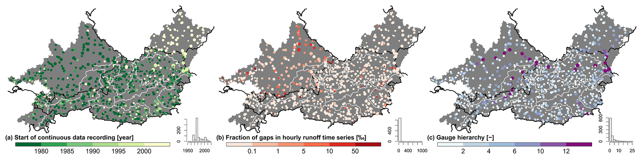
Figure 3 Maps showing a selection of gauge-referenced attributes. The size of the circles is proportional to the respective catchment area. The histograms indicate the number of gauges (out of 859) in each category. © EuroGeographics for the administrative boundaries.

Although the exact scope of data verification by the staff of the various hydrological services is not further specified, we have added an attribute describing the check status (“ckhs” in Table A1) to each time step of the runoff time series. The Austrian, Czech and Swiss runoff data are provided as exclusively checked, while the runoff data from the Bavarian hydrographic service are in most cases quality controlled until the years 2014, 2015 or 2016. Data from the German federal state Baden-Württemberg are often checked only from the year 2010 onwards. Some time series included gaps, even after checking by the hydrological services (“gaps_pre” in Table A1). Gaps of up to 6 h were filled with linear interpolation during our processing if the number of consecutive gaps was less than seven. Any remaining gaps (>6 h) were marked with the number −999. The fraction of remaining gaps in the continuous runoff time series is declared by the attribute “gaps_post” and illustrated in Fig. 3b. It is shown that those gauges with very few gaps (<0.1 ‰) are mostly located in Austria, the Czech Republic and Switzerland. About 80 % of the 882 gauges have no gaps in their continuous time series after our processing. The time steps with gaps before our processing are listed in separate files, attached to the dataset. The spatial distribution of the gauge hierarchy (see caption of Fig. 2b) is mapped in Fig. 3c., where 50 % of all gauges have a hierarchy of 1. The highest hierarchy (26) is found for the very last downstream gauge of the Austrian Danube (ID 399). Lastly, the attributes “nrs_euhyd” and “nrs_rivat” allow cross-references to the river network datasets EU-Hydro – River Network Database (EEA, 2019) and RiverATLAS (Linke et al., 2019), respectively. Thereby the ID of the river section corresponding to the gauge is given, enabling access to its attributes and routing through these networks.

4.2 Meteorological data

Given the extent of the ECMWF (European Centre for Medium-Range Weather Forecasts) ERA5-Land dataset with global coverage (Muñoz Sabater et al., 2021), it was possible to obtain gap-free time series with daily and hourly resolutions for 15 meteorological variables and 39 years (Table A2). ERA5-Land is a derivative of the ERA5 climate reanalysis (Hersbach et al., 2020) but only covers the terrestrial components. Further developments compared to ERA5 include an interpolation package for a finer temporal resolution and an additional sea level adjustment of the meteorological fields, as well as more efficient possibilities for the import of updates (Muñoz Sabater et al., 2021; Yang and Giusti, 2020). ERA5-Land has a spatial resolution of 0.1 arcdeg (about 9×11 km at the latitudes of the project area) compared to the grid size of ERA5 of 0.25 arcdeg. The temporal resolution of ERA5-Land is 1 h, while ERA5 only has a 3 h resolution. There is no data assimilation (fitting to observations) applied for ERA5-Land, but observations are indirectly implemented via the assimilated atmospheric fields of ERA5 (Hennermann and Guillory, 2020; Yang and Giusti, 2020). In accordance to ECMWF regulations, an uncertainty estimate for ERA5-Land will be released (Muñoz Sabater, 2019b; Muñoz Sabater et al., 2017).

Meteorological time series were computed for all three forms of basin delineation (A, B and C in Sect. 3). The aggregation was performed by calculating the area-weighted arithmetic mean (upscaling approach 1). As already mentioned in the Introduction, we would like to point out possible uncertainties in the published data. We therefore determined the components of the water balance for the period 1 October 1989 to 30 September 2009 (hydrological years 1990 to 2009) and plotted them (Fig. 4a). Values of catchments influenced by cross-basin water transfers, water withdrawals or intakes, large karstic springs, or high infiltration (Sect. 5.8) are not shown in Fig. 4a and c to allow a more objective interpretation. In the case of long-term water balances, it is usually feasible to neglect artificial storage in the catchment. The difference between long-term mean precipitation (P) and runoff height (Q), as recorded at the gauging station, should be equal to the total evapotranspiration (ETA) in a fulfilled water balance. This would be shown by having all points in Fig. 4a on the 1:1 line, which is not the case. Reasons for the rather strong scatter (Pearson correlation R=0.30) may be an insufficient representation of precipitation or total evapotranspiration by ERA5-Land; an inaccurate recording of runoff (e.g., strong, unrecorded groundwater flow or change in the river profile at the gauging station and thus an inadequate water level–discharge relationship); a significant deviation between the topographic and hydrographic catchment area (subsurface inflows and outflows, especially in karstic areas); or lastly, in the case of existing glaciers, a negative mass balance (Lambrecht and Kuhn, 2007; Kuhn, 2004; Kobolschnig and Schöner, 2011; Oerlemans et al., 1998; WGMS, 2005). Using other precipitation datasets for the same evaluation does not result in a significantly more compliant long-term water balance. CHIRPS Daily v2 (Funk et al., 2015) resulted in a correlation R between P − Q and ETA of 0.34 and MSWEP v2.2 (Beck et al., 2017, 2019) in even a lower R value of 0.26. Even if we cannot resolve the issue at hand, the total evapotranspiration from ERA5-Land and its dependence on elevation seem quite plausible compared to other studies (Fig. 4a; HAO, 2007, Map 3.3; Herrnegger et al., 2012, Fig. 20). Negative differences in mean precipitation and runoff height (Fig. 4a) and thus runoff coefficients >1.0 (Fig. 4c, 32 of 594 catchments) are mainly present in higher terrain (negative mass balance of glaciers, Fig. 8d) and in catchments with a high fraction of carbonate sedimentary rocks (indicator of karst, Fig. 11c). Since ERA5-Land indirectly incorporates in situ observational data via the assimilated atmospheric fields of ERA5 (Yang and Giusti, 2020), systematic measuring error of a terrestrial station being used could explain insufficient mean precipitation (Herrnegger et al., 2018). The individual components of the water balance are attached to the dataset for every catchment (Table A10) since this evaluation might be useful for explaining any deviations in a later modeling.

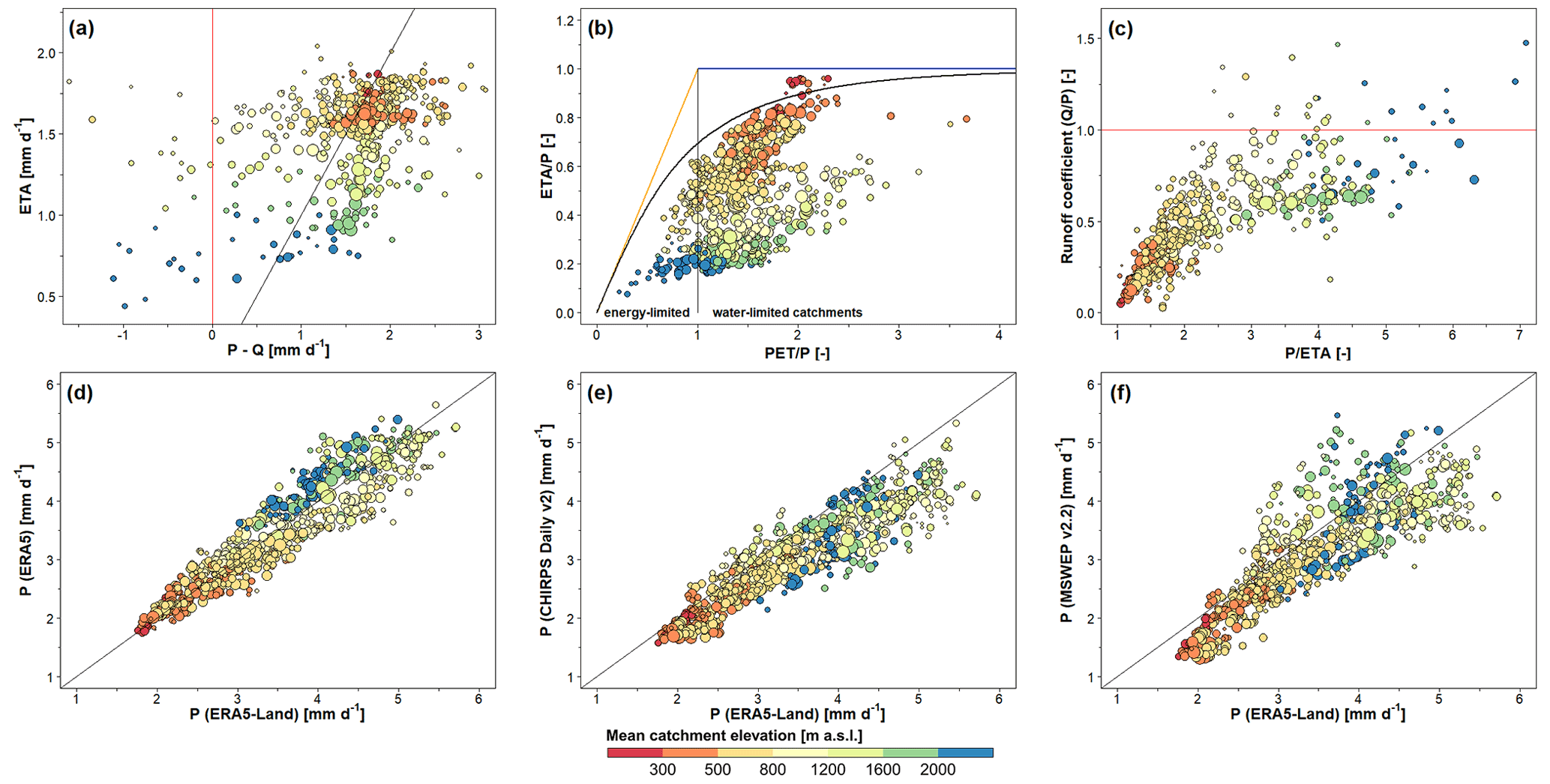
Figure 4 Analysis regarding the long-term water balance, evapotranspiration and comparison of the ERA5-Land's mean precipitation with other datasets for the hydrological years 1990–2009 and basin delineation A. (a) Total evapotranspiration (ETA) from ERA5-Land as a function of the difference between precipitation (P) from ERA5-Land and recorded runoff depth (Q). (b) Budyko curve indicates if ETA of a catchment is limited by energy (PET$/P<\mathrm{1}$) or by water (PET$/P>\mathrm{1}$). Panel (c) shows the runoff coefficient (ratio of Q and P) as a function of the fraction of ERA5-Land's precipitation and total evapotranspiration. In (a–c), values are only plotted for basins with observations for the period 1 October 1989 to 30 September 2009 (717 basins). Further, in (a, c), values are only plotted for basins not affected by artificial water input or withdrawal, karstic springs, or high infiltration (594 basins; Sect. 5.8). Plots (d, e and f) illustrate the relationship between ERA5-Land's precipitation compared to the datasets ERA5, CHIRPS Daily v2.0 and MSWEP v2.2 in 859 catchments. The diagonal black line in (a, d, e, f) is the 1:1 line. The red lines in (a, c) show physical constraints. The sloped orange line in (b) indicates the energy limit, while the horizontal blue line represents the water limit. The curved black line in (b) represents the Budyko curve. The size of the symbols in all plots is proportional to the catchment area, while the color indicates the mean elevation of the catchment (see legend at bottom).

The Budyko curve (Fig. 4b; Budyko, 1974) describes the relationship between the ratio of total evapotranspiration $/$ precipitation (ETA $/P$) and the ratio of potential evapotranspiration $/$ precipitation (PET $/P$) and indicates whether evapotranspiration of a catchment is limited by energy or water. Ideally all points should lie in the proximity of the Budyko curve. The deviation from this ideal case can primarily be explained by a PET of ERA5-Land over nearly the entire range of elevation that is significantly too high. For example, 98 % of all 859 watersheds show mean annual PET sums above 1000 mm (“PET” in Table A10). As these PET sums are not realistic at the latitudes of the project area (HAO, 2007, Map 3.2; Herrnegger et al., 2012, Fig. 17), we did not include PET time series of ERA5-Land in the LamaH dataset. However, there is the possibility of obtaining daily PET time series from provided fluxes of the hydrological model (Sect. 6, Table C2). The runoff coefficient ($Q/P$) as a function of the ratio of mean precipitation $/$ total evapotranspiration ($P/$ ETA) is shown in Fig. 4c. The altitudinal dependency can be clearly seen in Fig. 4c, while catchments with lower mean elevation show less scatter. Figure 4d shows the contrast of the long-term precipitation of ERA5-Land with those of ERA5 (Pearson correlation R=0.936). ERA5 indicates systematic surplus of precipitation at catchments with mean altitudes above 2000 $\mathrm{m}\mathrm{a}.\mathrm{s}.\mathrm{l}.$ compared to ERA5-Land, while at catchments with mean altitudes between 800 and 1200 $\mathrm{m}\mathrm{a}.\mathrm{s}.\mathrm{l}.$ the opposite is more likely to be the case. The correlation between the long-term precipitation of ERA5-Land and those of the dataset CHIRPS daily v2 (Funk et al., 2015) is 0.916 (Fig. 4e). Further, the mean precipitation sums of CHIRPS daily v2 tend to be lower than those of ERA5-Land over the whole range of altitudes. More scatter (R=0.841) appears especially in catchments with higher elevations when comparing the long-term precipitation sums of ERA5-Land and MSWEP v2.2 (Beck et al., 2017, 2019; Fig. 4f).

5 Catchment attributes

The various physio-geographical characteristics of a catchment, as well as their interactions, are essential for water storage and transport on and below Earth's surface (Blöschl et al., 2013). The spectrum of influencing catchment characteristics includes topography, climate, hydrology, land cover, vegetation, soil and geology, as well as the type and degree of (anthropogenic) impact on runoff processes. Furthermore, catchment attributes are crucial to determine interrelationships among different watersheds along several gradients (Addor et al., 2017; Falkenmark and Chapman, 1989; Fan et al., 2019).

In most cases, we used freely available datasets with global or at least European coverage for deriving the different catchment attributes. The datasets used for deriving the attributes, methods of processing and possible uncertainties as well as the spatial distribution of catchment attributes (Addor, 2017) are discussed in more detail in the following subsections. It is clear that due to the large extent of LamaH, this account is far from complete. The individual attributes are listed in tabular form in the Appendix A with a more detailed description, units and reference to the data sources.

5.1 Topographic indices

We calculated 10 topographic attributes, which are listed in Table A3. The attribute area_calc describes the calculated aggregation (catchment) area, depending on the applied method of basin delineation (Sect. 3). A key factor for hydrological processes is elevation, as it affects numerous other catchment characteristics including climate, land cover, vegetation or soil development (Addor et al., 2017). We derived the mean catchment elevation (Fig. 5b, “elev_mean” in Table A3), the median elevation (“elev_med”), standard deviation within a catchment (“elev_std”) and the elevation range (maximum − minimum elevation in the catchment, Fig. 5c, “elev_ran”), as well as the mean catchment slope (Fig. 5d, “slope_mean”) from NASA's SRTM dataset (Farr et al., 2007). SRTM features a grid size of 30 m and provides a maximum global absolute vertical error of 16 m at a 90 % confidence interval while accuracy decreases with increasing elevation and slope (Farr et al., 2007). The slope was calculated with the algorithm of Horn (1981) using the terrain elevation from SRTM. High mean catchment elevations and slopes are most apparent in the Eastern Alps, which extend from the southwest to the central east of the project area. This highly elevated area is mainly surrounded by the flatter Alpine foothills and regions with older geological zones (Fig. 5b).

Figure 5 Spatial distribution of a selection of topographic attributes representing the characteristics of the entire topographic catchment (basin delineation A, Fig. 2a). The histograms indicate the number of basins (out of 859) in each category. The size of the circles is proportional to the catchment area. © EuroGeographics for the administrative boundaries.

The shape of the catchment and the stream network influence runoff formation. The direction of precipitation in relation to the longitudinal axis of the catchment is of major interest in the case of flood situations, especially in larger catchments. For this reason, we specified the angle between the north direction and the longitudinal axis (“mvert_ang”) in addition to the distance of the longitudinal axis of a catchment (“mvert_dist”). In combination with the two wind components of ERA5-Land (“10m_wind_u” and “10m_wind_v” in Table A2) it is possible to derive the relative rainfall trajectory. The attribute of length elongation according to Schumm (1956) (Fig. 5e, “elon_ratio”) is an indicator regarding the “roundness” (the higher, the rounder) of the catchment. Stream density (Fig. 5f, “strm_dens”) is a function of several characteristics (e.g., climate, relief, soil properties, geology, vegetation, land use, glaciation or karstification) and can therefore be an informative indicator for comparing watersheds (Olden and Poff, 2003). The EU-Hydro – River Network Database (EEA, 2019) is used for calculating the stream density, since it is a finely resolved dataset and consistent over the project area covered.

5.2 Climatic indices

LamaH includes 12 attributes reflecting aspects of climatic characteristics (Table A4). These attributes were calculated mainly from the meteorological time series of ERA5-Land for the period 1 October 1989 to 30 September 2009 (Addor, 2017). The reference evapotranspiration (ET0) from the Global Aridity Index and Potential Evapotranspiration (ET0) Climate Database v2 (GCD v2; Trabucco and Zomer, 2019), which was computed for the period 1970 to 2000, is provided as an alternative to ERA5-Land's potential evapotranspiration, which shows unrealistically high values (Sect. 4.2). ET0 describes the atmosphere's capacity for evapotranspiration given defined vegetation characteristics. Potential evapotranspiration (PET) can be derived from ET0 using correction factors for vegetation and soil properties (Allen et al., 1998; Hargreaves, 1994) but was not realized in LamaH.

Long-term climatic characteristics are described by long-term daily precipitation (Fig. 6a, “p_mean” in Table A4), reference evapotranspiration (Fig. 6b, “et0_mean”), total evapotranspiration (“eta_mean”), and the aridity index (Fig. 6c, “arid_2”). As an alternative, the aridity index which was calculated by dividing ET0 from GCD v2 by precipitation from ERA5-Land is also included (“arid_1”). The spatial pattern of long-term precipitation sums (Fig. 6a) clearly shows an elevation gradient and blocking effects along the northern Alps. The west of the project area is characterized by higher mean precipitation due to the stronger influence of oceanic climate. The relationships between mean catchment elevation (Fig. 5b) and ET0 (Fig. 6b, Pearson correlation $R=-\mathrm{0.79}$), aridity (Fig. 6c, $R=-\mathrm{0.68}$) or the fraction of precipitation falling as snow (Fig. 6g, R=0.96) show similar spatial patterns. About 19 % of all catchments, which are exclusively located in the eastern part of the project area, have aridity greater than 1 (arid_2).

Figure 6 Spatial distribution of a selection of climate indices representing the characteristics of the entire topographic catchment (basin delineation A, Fig. 2a). The histograms indicate the number of basins (out of 859) in each category. The size of the circles is proportional to the catchment area. © EuroGeographics for the administrative boundaries.

Attributes characterizing seasonality are the fraction of precipitation falling as snow (Fig. 6g, “frac_snow”) and the seasonality index, which relies on sinusoids to describe the precipitation cycle over the year (Fig. 6d, “p_season”). A higher positive seasonality index indicates higher precipitation sums during summer, while values near 0 show a more balanced precipitation distribution throughout the year.

While long-term and seasonal indices describe general climatology, they provide little or no information about relatively short-term events such as drought or heavy rainfall. Consequently, we calculated attributes representing the frequency of high-precipitation days (days per year with at least 5 times the mean daily precipitation; Fig. 6e, “hi_prec_fr”) and dry days (days per year with max 1 mm d⁻¹ precipitation; Fig. 6h, “lo_prec_fr”), their mean duration (Fig. 6f, “hi_prec_du”, and Fig. 6i, “lo_prec_du”), and the most likely season of occurrence (“hi_prec_ti” and “lo_prec_ti”). The reason for the higher frequency of high-precipitation days in the southeastern part of the project area (Fig. 6e) is primarily the combination of convective precipitation events during the summer months relatively rich in rainfall and relatively low precipitation sums during the rest of the year (Fig. 6d). For both the mean frequency of dry days (Fig. 6h, $R=-\mathrm{0.62}$) and their mean duration (Fig. 6i, $R=-\mathrm{0.57}$), a negative spatial correlation with the mean catchment elevation (Fig. 5b) can be observed. The most common season for high precipitation for 89 % of all 859 catchments is summer (June, July and August), while winter (December, January and February) is the most common season for dry days in 89 % of the basins.

5.3 Hydrological signatures

The runoff time series are characterized by 14 attributes (Table A5) which were calculated for the period 1 October 1989 to 30 September 2009 (Addor, 2017). The indices were computed for those gauges which cover the whole period of investigation (717 gauges). However, evaluations for the entire period of record (from the first 1 October after 1981 to 30 September 2017) are additionally made available if at least 5 full hydrological years are recorded. Four gauges do not meet this requirement. Hydrological signatures are calculated only if the fraction of gaps is less than 5 % for both evaluation periods. Hydrological attributes can be divided into those describing long-term characteristics, seasonality, and more short-term situations such as high and low flow.

Aridity by itself can be a good predictor of runoff occurrence in a catchment (Arora, 2002; Blöschl et al., 2013; Budyko, 1974). This is shown by the similar spatial pattern of long-term runoff height (Fig. 7a, “q_mean” in Table A5, $R=-\mathrm{0.61}$) and runoff ratio (Fig. 7b, “runoff_ratio”, $R=-\mathrm{0.60}$) compared to those of aridity (Fig. 6c). The runoff coefficient ($Q/P$) is the fraction of precipitation that drains a surface after deducting evapotranspiration, groundwater flow or change in storage in the long term. Explanations for runoff coefficients greater than 1 are given in Sect. 4.2. The ratio of baseflow and total runoff can be a useful indicator for watershed classification (Sawicz et al., 2011; Fan, 2015) and is further referred to as the baseflow index (“baseflow_index”). It should be noted that this index is highly dependent on the method used to separate the hydrograph (Beck et al., 2013; Chapman, 1999; Eckhardt, 2008). For this reason, we used the Ladson filter (Ladson et al., 2013) and the approach of Tallaksen and Van Lanen (2004) for hydrograph separation. The runoff–precipitation elasticity (“stream_elas”) characterizes the inertia of change in mean runoff given a change in mean precipitation (Sankarasubramanian et al., 2001). For example, a value of 3 would indicate a change in runoff of 3 % given a change in precipitation of 1 %. High runoff–precipitation elasticity is especially present in the eastern part of the project area (Fig. 7f). The fraction of days without discharge (not shown, “zero_q_freq”) may indicate strong infiltration (e.g., Danube Sinkhole; Hötzl, 1996), artificial water withdrawal or ceasing baseflow.

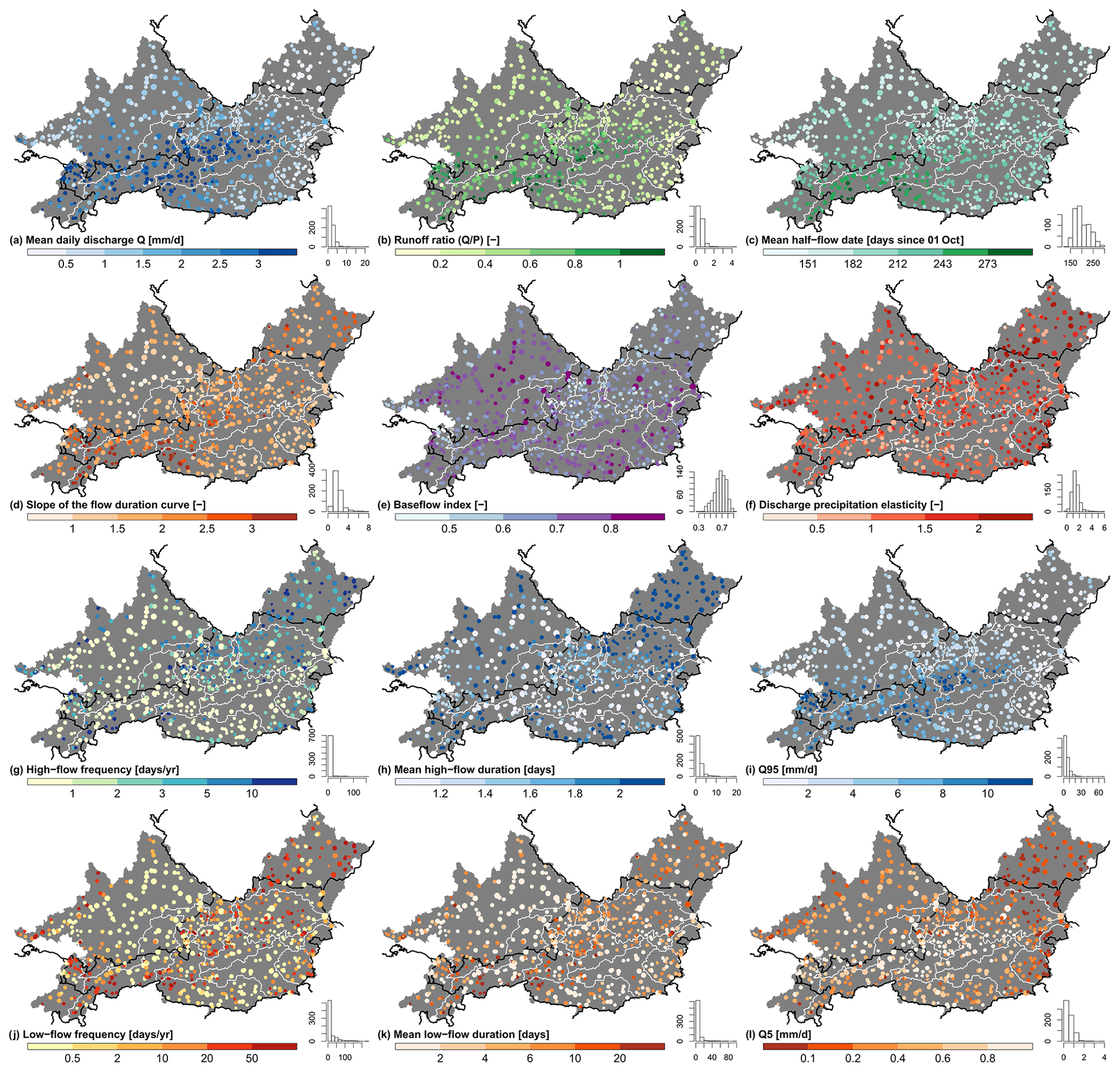
Figure 7 Spatial distribution of hydrological signatures. Only gauges are plotted which cover the period 1 October 1989 to 30 September 2009. The histograms indicate the number of gauges (out of 717) in each category. The size of the circles is proportional to the catchment area. © EuroGeographics for the administrative boundaries.

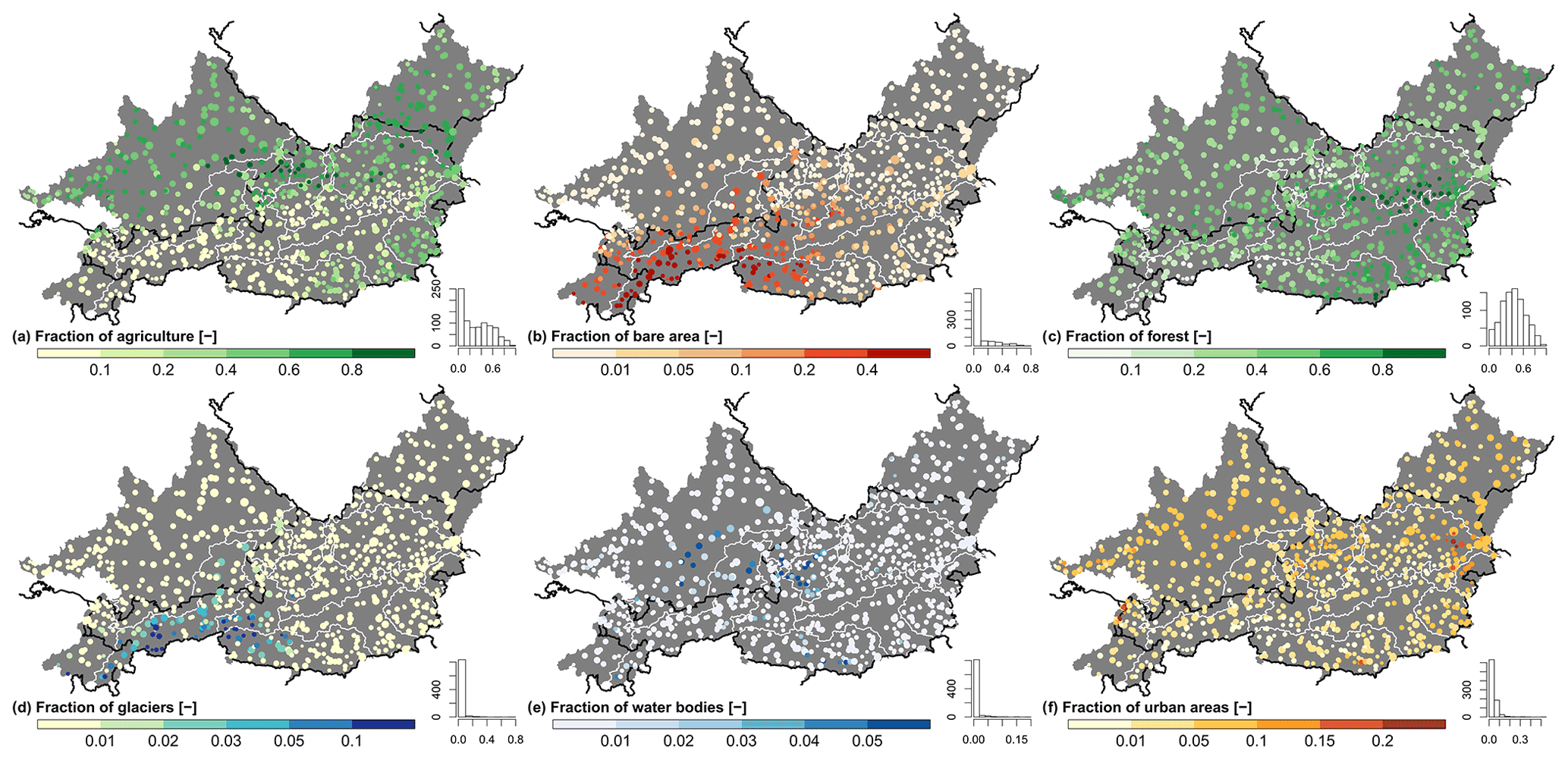
Figure 8 Spatial distribution of land class fractions representing the characteristics of the entire topographic catchment (basin delineation A, Fig. 2a). The histograms indicate the number of basins (out of 859) in each category. The size of the circles is proportional to the catchment area. © EuroGeographics for the administrative boundaries.

The seasonality of runoff is expressed by the attribute “hfd_mean”, which shows the number of days from the beginning of the hydrological year (1 October) to the date when half of the annual runoff volume is reached (Court, 1962). The higher number of days in Fig. 7c can be explained primarily by water storage in the form of snow (Fig. 6g) or glaciers (Fig. 8d). Variability in runoff (Fig. 7d, “slope_fdc”) is expressed within LamaH by the slope of the flow duration curve between the log-transformed 33rd and 66th runoff percentiles (Sawicz et al., 2011). High values are indicative of high runoff variability over the year, which can be caused by seasonal water storage in the form of snow (Fig. 6g) or a strong response of runoff to precipitation (Yokoo and Sivapalan, 2011).

Extreme runoff events such as high or low flow are described by indices representing mean frequency (Fig. 7g, “high_q_freq”, and Fig. 7j, “low_q_freq”), duration (Fig. 7h, “high_q_dur”, and Fig. 7k, “low_q_dur”) and magnitude. The threshold for high flow (at least 9 times the median daily discharge) is chosen according to Clausen and Biggs (2000) and that for low flow (max 0.2 times the median daily discharge) according to Olden and Poff (2003). The magnitudes of extreme flows are expressed by the 95th (high flow, Fig. 7i, “Q₉₅”) and the 5th (low flow, Fig. 7l, “Q₅”) runoff percentiles. The hydrological indices (Fig. 7) are spatially less smoothly distributed compared to the climatic indices (Fig. 6). The reasons might be the influence of the (non-)linear hydrological processes by locally heterogeneous catchment characteristics or uncertainties in runoff measurement (Addor et al., 2017; Westerberg et al., 2016).

5.4 Land cover characteristics

All attributes concerning land class (Table A6) are based on the CORINE Land Cover (CLC) 2012 raster dataset featuring a grid size of 100 m (CORINE, 2012). CORINE is an initiative of the European Environment Agency with the aim to record land cover of the European territory with a 6-year update cycle. The basic technical specifications like 44 land classes, a 25 ha minimum mapping unit (MMU) for areal phenomena and a 100 m minimum width for linear phenomena have not changed since the beginning, facilitating comparisons over the years (CORINE, 2012). It should be noted that an MMU of 25 ha prevents mapping of very small scaled structures. Other limitations might be the variability in satellite image quality and contents, difficulties in setting up automatic conversion processes, and the difference between human interpretation capacity and pixel-based classification (Bossard et al., 2000). However, the total reliability of the predecessor dataset CLC 2000 is 87.0±0.8 % according to a reinterpretation approach. The worst class-level reliability (<70 %) was found for sparse vegetation (CLC class 333) (Büttner and Maucha, 2006). The dominant land class within a basin delineation is derived by the majority of the intersecting raster centroids, while the fractions are derived by area share of the specific raster cells.

Agricultural land (Fig. 8a, “agr_fra” in Table A6) has high fractions in catchments with a low mean slope (Fig. 5d, $R=-\mathrm{0.89}$). The opposite occurs for the fraction of bare areas (Fig. 8b, “bare_fra”), since the vegetation period is very short at highly elevated terrain and a high terrain slope fosters gravitational erosion processes. Following the CAMELS datasets, no differentiation was made between deciduous and coniferous forests when calculating the forest share. The proportion of forest is highest in the central eastern region of the project area (Fig. 8c, “forest_fra”), where agriculture and settlement are less prevalent and the mountains are often lower than the forest line. Catchments with a relatively high proportion of glaciers (Fig. 8d, “glac_fra”) are mainly located in the western Eastern Alps. The influence of glaciers upon the hydrological regime is primarily apparent in the upper parts of the river regions Inn (region 3 in Fig. 1 and Table B1), Salzach (region 4) and Drava (region 18). High proportions of water surface (Fig. 8e, “lake_fra”) can be explained by large lakes, which were mostly formed at the end of the last great ice age about 10 000 years ago (mainly in the Alpine foothills) or by large artificial water reservoirs (mainly in the Czech Republic). Catchments in the Vienna metropolitan area (eastern part of river region 10), as well as in the lower Rhine valley (northern part of river region 1), show quite high fractions of urban area (Fig. 8f, “urban_fra”). However, most catchments (about 74 %) have less than 5 % urban area.

5.5 Vegetation indices

We calculated six catchment attributes describing vegetation indices, which are based on leaf area index (LAI), normalized difference vegetation index (NDVI) and green vegetation fraction (GVF) (Table A7). All vegetation indices are based on long-term monthly means, using the maximum, minimum, or difference between the maximum and minimum monthly means (based on 12-monthly means). Processing of the remote sensing datasets was performed using the Google Earth Engine platform (GEE, 2021a, b; Gorelick et al., 2017).

LAI represents vertical vegetation density and is defined as the sum of the one-sided green leaf area per unit area for deciduous forests and half of the total needle area per unit area for coniferous forests. LAI was derived from the MODIS MCD15A3H dataset, which is a 4 d composition with a 500 m grid resolution (Myneni et al., 2015). The maximum and minimum monthly means were calculated for the period 1 August 2002 to 1 January 2020 using a cloud filter. The maximum monthly mean of LAI (Fig. 9a, “lai_max” in Table A7) and the difference between maximum and minimum (Fig. 9d, “lai_diff”) show a spatial correlation with the forest fraction (Fig. 8c, R=0.76 and R=0.75, respectively). LAI_diff shows the same values as LAI_max for large parts of the project area. Especially in regions characterized by a high proportion of coniferous forest, the LAI_diff should be smaller than LAI_max due to the permanent green cover. Snow cover during the winter months could be a possible reason for the non-representative measurement of the minimum values of LAI.

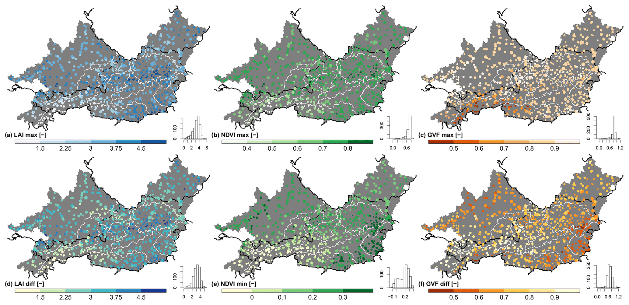
Figure 9 Spatial distribution of vegetation indices representing the characteristics of the entire topographic catchment (basin delineation A, Fig. 2a). The histograms indicate the number of basins (out of 859) in each category. The size of the circles is proportional to the catchment area. © EuroGeographics for the administrative boundaries.

NDVI is derived from the backscatter of two spectral bands and is widely used for remote-sensing-based vegetation monitoring and classification (horizontal density, type and physiological condition). The maximum and minimum monthly NDVI is based on the MODIS MOD09Q1 dataset with a temporal resolution of 8 d and a spatial resolution of 250 m (Vermote, 2015). The calculation was performed for the period 1 April 2000 to 1 January 2020, applying a filter to cloudy satellite images. A negative correlation is apparent between the NDVI_max (Fig. 9b, “ndvi_max”, $R=-\mathrm{0.78}$) or the NDVI_min (Fig. 9e, “ndvi_min”, $R=-\mathrm{0.84}$) and the mean catchment elevation (Fig. 5b).

GVF (green vegetation fraction) indicates the fraction of soil that is covered by green vegetation and can be derived from the NDVI as follows in Eq. (1) (Broxton et al., 2014):

$$\begin{array}{}\text{(1)}& {\displaystyle }{\displaystyle }\text{GVF}={\displaystyle \frac{\text{NDVI}-{\text{NDVI}}_{\mathrm{s}}}{{\text{NDVI}}_{\text{c,v}}-{\text{NDVI}}_{\mathrm{s}}}},\end{array}$$

where NDVI represents the (maximum or minimum) monthly mean of NDVI, NDVI_s the annual maximum NDVI of bare ground and NDVI_c,v the annual maximum of vegetated ground surface as a function of IGBP land class (Table 1 in Broxton et al., 2014). NDVI_s was set to 0.09 in accordance with Broxton et al. (2014), while the spatial distribution of the IGBP land classes was obtained from the MODIS MCD12Q1 dataset of the year 2012 (Friedl and Sulla-Menashe, 2019). As the values for NDVI_s and NDVI_c,v were derived for a global scale and thus do not necessarily correspond to conditions in the project area, it is possible for GVF values to exceed the normal range between 0 and 1. In order to maintain consistency, we did not constrain the GVF to the normal range, however. The spatial distribution of GVF_max (Fig. 9c, “gvf_max”) shows similar spatial patterns to those of LAI_max (R=0.79) as well as NDVI_max (R=0.94), while GVF_diff (Fig. 9f, “gvf_diff”) tends to be higher in regions with a higher fraction of precipitation falling as snow (Fig. 6g).

5.6 Soil characteristics

LamaH includes 10 attributes to characterize soil properties (Table A8), where 8 of them are derived from the 1 km grid sized European Soil Database Derived data (ESDD; Hiederer, 2013a, b). ESDD is based on the European Soil Database (ESD; Panagos et al., 2012; Panagos, 2006), while the maximum available soil water content (TAWC) in ESDD was calculated using pedotransfer functions (Hiederer, 2013a). ESDD provides soil attributes for a topsoil layer and a subsoil layer having the boundary at 30 cm soil depth. Values from these two layers were therefore aggregated and weighted by the available root depth (“root_dep” in Table A8) or in the case of TAWC summed up. The attribute describing the depth to bedrock “bdrk_dep” is based on the layer “average soil and sedimentary deposit thickness” of the dataset Global 1-km Gridded Thickness of Soil, Regolith, and Sedimentary Deposit Layers (GGT; Pelletier et al., 2016). GGT has a spatial resolution of 30 arcsec (approximately 1 km) and is derived from landform-specific models (for upland, lowland, slope and valley floor) considering geomorphological principles and incorporating data for topography, climate and geology. Calibration and validation in GGT were performed using independent borehole profiles (Pelletier et al., 2016). The 3D Soil Hydraulic Database of Europe (3DSHD; Toth et al., 2017) dataset with a grid size of 250 m served as the source for extracting the saturated hydraulic soil conductivity (“soil_condu”). It was derived using pedotransfer functions (Toth et al., 2015) incorporating attributes from the SoilGrids250m dataset (SG250; Hengl et al., 2017), and SG250 is based on machine learning techniques including data from about 150 000 soil profiles as well as remote sensing data for climate, vegetation, geomorphology and lithology (Hengl et al., 2017). Data within 3DSHD are provided for seven soil layers, so depth-weighted harmonic averaging was applied.

The provided soil attributes in LamaH may include large uncertainties and should therefore be considered with caution for several reasons. First, the soil attributes from ESD are mainly based on extrapolated observations of soil profiles and expert estimates (ESDB, 2004). Especially in the case of heterogeneous soil conditions and large distances between soil profiles, the reliability of the ESD dataset must be treated with caution. Data from soil profiles are integrated into 3DSHD (Hengl et al., 2017; Toth et al., 2017) and the dataset of Pelletier et al. (2016) as well but are rather used for calibration and validation. Toth et al. (2017) indicate increased unreliability for 3DSHD above 1000 $\mathrm{m}\mathrm{a}.\mathrm{s}.\mathrm{l}.$ (about 24.2 % of the project area is above 1000 $\mathrm{m}\mathrm{a}.\mathrm{s}.\mathrm{l}.$). Furthermore, the limitation of the soil depth at 1.5 m in ESDD and 2.0 m in 3DSHD is another source of uncertainty (Boer-Euser et al., 2016). As a last point, it must be mentioned that much spatially distributed information is lost by aggregation to the basin scale.

Figure 10 Spatial distribution of soil attributes representing the characteristics of the entire topographic catchment (basin delineation A, Fig. 2a). The histograms indicate the number of basins (out of 859) in each category. The size of the circles is proportional to the catchment area. © EuroGeographics for the administrative boundaries.

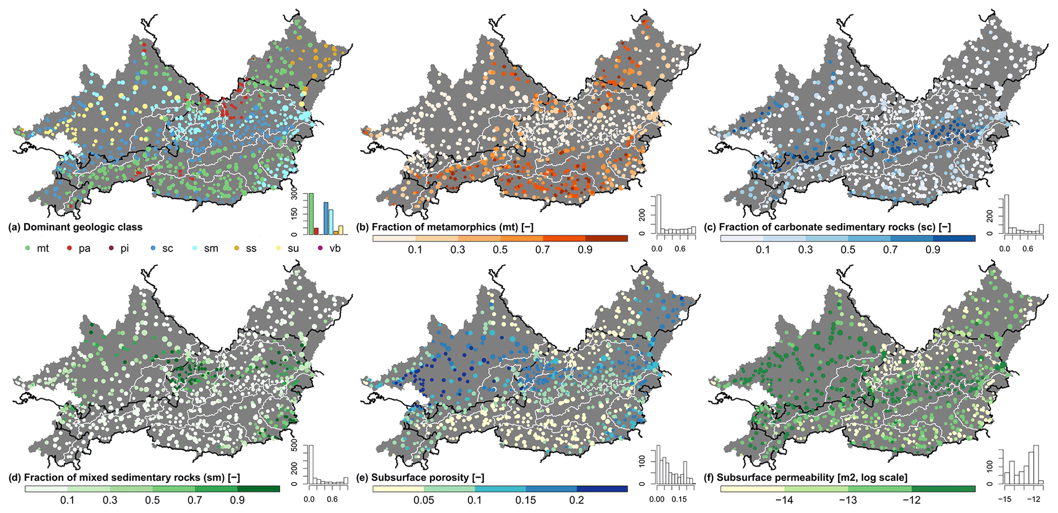
Figure 11 Spatial distribution of geological attributes representing the characteristics of the entire topographic catchment (basin delineation A, Fig. 2a). The histograms indicate the number of basins (out of 859) in each category. The size of the circles is proportional to the catchment area. Classes in plot (a): mt – metamorphites, pa – acid plutonic rocks, pi – intermediate plutonic rocks, sc – carbonate sedimentary rocks, sm – mixed sedimentary rocks, ss – siliciclastic sedimentary rocks, su – unconsolidated sediments, vb – basic volcanic rocks. © EuroGeographics for the administrative boundaries.

Depth to bedrock (Fig. 10a, “bedrk_dep” in Table A8) shows similar spatial patterns to mean catchment slope (Fig. 5d, $R=-\mathrm{0.56}$) and mean elevation (Fig. 5b, $R=-\mathrm{0.46}$). About 37 % of all 859 catchments have a mean depth to bedrock of more than 1.5 m. This depth represents the maximum root-available depth in ESDD (Fig. 10b, root_dep). The depth available for roots tends to be higher in Germany and the Czech Republic than in other regions. Whether this is an indication of different measurement methods across the countries is unclear. Low available rooting depths in Austria are, according to Fig. 10b, mainly present where the fraction of carbonate sedimentary rocks (Fig. 11c) or glaciers (Fig. 8d) is high. Of all catchments, 40 % exhibit a mean organic soil content below 1 %, while the highest organic contents are located in the southern German region (Fig. 10c, “oc_fra”). Further interrelationships between the various grain size fractions and the dominating bedrock are recognizable: (1) a high proportion of sand (Fig. 10d, “sand_fra”) is especially prevalent where the fraction of metamorphic bedrock is high (Fig. 11b, R=0.47). (2) Moreover, the fraction of silt (Fig. 10e, “silt_fra”) tends to be high at the catchment level where a high fraction of carbonate sedimentary rock (Fig. 11c, R=0.52) is present. (3) Finally, we can observe an increase in clay content (Fig. 10f, “clay_fra”) with an increasing proportion of mixed sedimentary rock (Fig. 11d, R=0.47). Soil porosity (Fig. 10g, “soil_poros”) shows similar spatial patterns compared to the sand fraction ($R=-\mathrm{0.79}$), while saturated hydraulic conductivity (Fig. 10h, soil_condu) tends to increase with decreasing mean catchment elevation (Fig. 5b, $R=-\mathrm{0.63}$). The available soil water content (TAWC, “soil_tawc”) was determined in ESDD by including water content at field capacity, gravel content and root-available depth (Hiederer, 2013a). That explains the high correlation of TAWC (Fig. 10i) with the root-available soil depth (Fig. 10b, R=0.94).

5.7 Geological characteristics

We used the datasets GLiM (Hartmann and Moosdorf, 2012; Global Lithological Map) and GLHYMPS (Gleeson et al., 2014; GLobal HYdrogeology MaPS) for deriving 16 geological attributes (Table A9). GLiM summarizes 92 regional geological maps in vector form and was used to extract the fractions of the different geological classes. GLiM offers three levels of detail, with the first-level species the dominant lithologic class. The optional second as well as third level further specifies, for example, the structure of the rock or local conditions (Hartmann and Moosdorf, 2012). For LamaH only the first level of GLiM was used, which contains 16 geological classes. The classes “evaporites”, “no data” and “intermediate volcanic rocks” do not occur within the project area. The three most common dominant geological classes (Fig. 11a, “gc_dom” in Table A9) across all 859 catchments are metamorphites (mt, 35.1 %), carbonate sedimentary rocks (sc, 27.4 %) and mixed sedimentary rocks (sm, 21.2 %). Metamorphic rocks (Fig. 11b, “gc_mt_fra”) are predominant along the northern border of the project area (Bohemian Massif), as well as in the more southern project area (central Eastern Alps), and include mainly schist, gneiss and quartzite. From a hydrological point of view, the proportion of carbonate sedimentary rock is of particular interest since a high fraction can be an indicator for karstic systems. High shares of carbonate sedimentary rocks are mainly found along the belt from the southwest to the central east of the project area (Northern Limestone Alps), the central southern border (Southern Limestone Alps) and the northeastern border (Swabian Alb) (Fig. 11c, “gc_sc_fra”). The flysch and molasse zone (Alpine foothills and central parts of the German project area) is basically characterized by a high fraction of mixed sedimentary rocks (Fig. 11d, “gc_sm_fra”).

Attributes concerning permeability and porosity of the lithologic bedrock were extracted from GLHYMPS. There is a high spatial correlation between GLHYMPS and GLiM, as geological classes of GLiM served as a starting point for assigning hydraulic properties in GLHYMPS. Huscroft et al. (2018) declare that permeability in GLHYMPS is determined only for saturated conditions. GLHYMPS is only intended for regional-scale applications (i.e., spatial resolutions greater than 5 km), as the influence of local heterogeneities such as fault zones can be neglected above this scale (Gleeson et al., 2014).

A high proportion of metamorphites or plutonites (mt, pa and pi in Fig. 11a) is commonly associated with low bedrock porosity (Fig. 11e, “geol_poros”). Catchments within the flysch and molasse zones in contrast exhibit relatively high porosity. High bedrock porosity is not necessarily followed by high subsurface permeability (“geol_perme”), yielding a much more inhomogeneous spatial pattern in Fig. 11f than in Fig. 11e. The reason may be rock structure (second stage of GLiM), which can have different impacts on permeability and porosity (Table 1 in Gleeson et al., 2014).

5.8 Information on (anthropogenic) impacts on runoff processes and measurements

We provide four attributes (Table 1) in order to simplify filtering and evaluation of time series of runoff gauges regarding any (anthropogenic) impact on runoff processes or its measurement. We have represented the diversity of (human) impact by 13 types of impact (“typimpact” in Table 1). The type of (human) impact on runoff or measurement was determined primarily from gauge metadata declared by hydrographic services (BAFU, 2020; GKD, 2020; HZB, 2020; LUBW, 2020). Additionally, publicly available information, as well as manual aerial photo evaluations, was used for determination. Typical types of human impact in the project area are large water reservoirs often associated with hydropower plants and cross-basin water transfers. The following types of influence were not classified because the necessary information is not consistently available or is only available with great effort: (1) icing, especially at smaller rivers in winter; (2) variable channel profiles leading to inaccurate rating curves; (3) high groundwater flow in the area around the gauge; and (4) subsurface transboundary in- or outflows especially in highly karstified areas.

Table 1 Attributes for (anthropogenic) gauge and catchment interference.

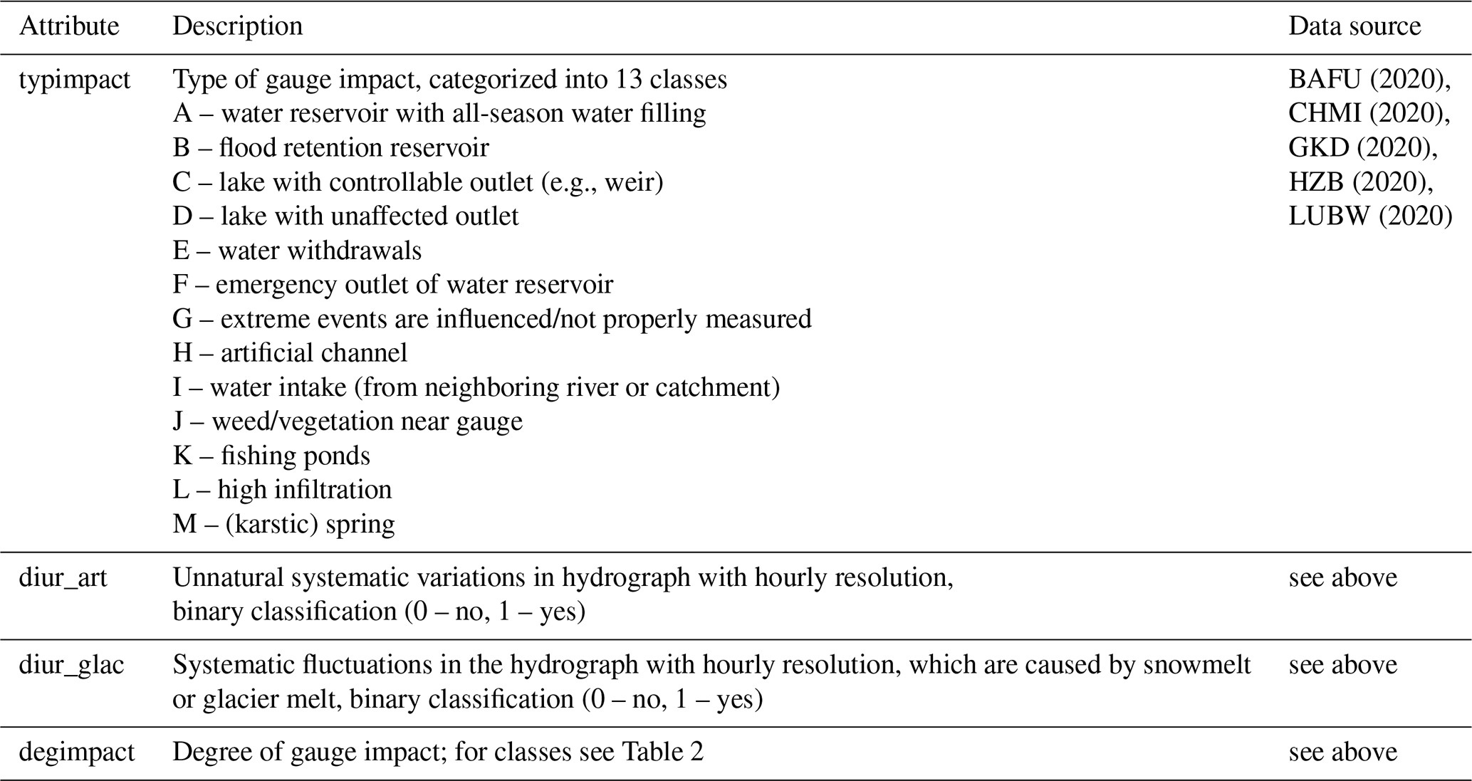
The hydrographs with an hourly resolution in the months of January and July for the years 1990, 2005 and 2017 were additionally manually evaluated regarding systematic diurnal variations (“diur_art” and “diur_glac” in Table 1). Systematic fluctuations were further subdivided into those caused artificially (e.g., by storage power plants, power plants with swell operation or sewage treatment plants) and those caused naturally (snowmelt or glacier melt). Summarizing the influences for every time series, the degree of gauge impact (“degimpact”) is determined mostly based on the type of impact and any systematic diurnal variations (Table 2). Obviously, a gauge or catchment area can be characterized by several types of impact. In such cases, the highest degree of impact was chosen. Geo-localization of the impacts is provided by the shapefile Impacts.shp, which includes links to the dam datasets GRanD (“GRAND_ID”; Lehner et al., 2011) and GOODD (“DAM_ID”; Mulligan et al., 2020) to ensure fast access to those attributes.

Table 2 Criteria for the different degrees of gauge impact.

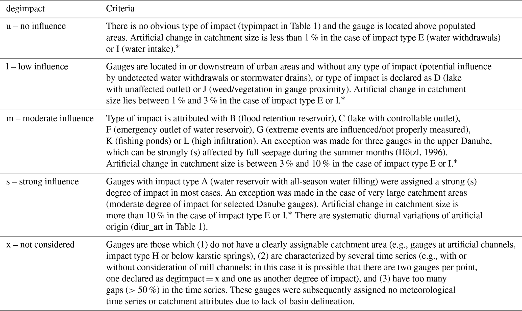
^* The hydrographic yearbook of Austria declares anthropogenic cross-basin water transfers by increasing or decreasing the natural catchment area of a gauge (BMLFUW, 2013). There is no information regarding artificial changes in catchment size for gauges outside Austria. Here, the degree of impact was additionally determined, and it was also determined at Austrian gauges influenced by other kinds of water withdrawal (river branches, diversions or irrigation), on the basis of publicly available information as well as aerial photo analyses. We thereby mostly assigned a strong degree of impact (s) but in a few cases (e.g., withdrawals for drinking water) also a moderate degree (m).

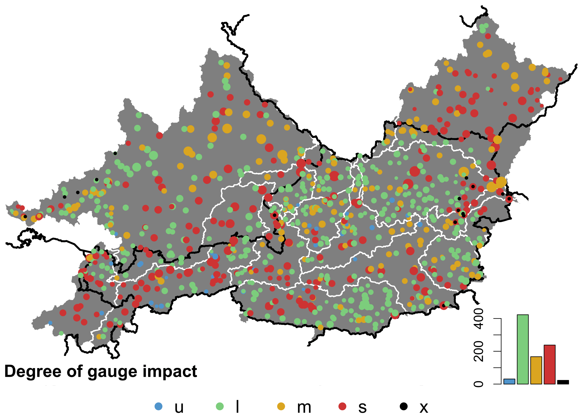
Figure 12 Degree of (anthropogenic) impact on gauges/catchments. The histogram indicates the number of gauges (out of 882) in each category. The size of the circles is proportional to the catchment area. Classes: u – no influence, l – low influence, m – moderate influence, s – strong influence, x – not considered in basin delineation. © EuroGeographics for the administrative boundaries.

The spatial, as well as the frequency, distribution of the degree of impact is shown in Fig. 12. Of 882 gauges, 3.5 % are not influenced (u), 48 % show a low influence (l), 18.9 % are moderately influenced (m) and 27 % are strongly influenced (s), while 2.6 % belong to class x. Low-influenced gauges are predominant in the northwest of the German project area, in the north of the Austrian central region (river region 5, 6, 7, 8, 9 and 10 in Fig. 1) and in the east (river region 16), as well as in the south of Austria (east of river region 18). Strongly influenced gauges are in contrast mainly prevalent where large water reservoirs are in operation for hydropower generation (primarily in the Alpine region) and for seasonal water balancing or flood protection (primarily in the Czech Republic and in the north of the German project area). It should be noted that gauges located far downstream of large reservoirs may still be strongly influenced by them.

6 Hydrological model

6.1 Model setup

Finally, we set up a conceptual hydrological model in order to check the inputs for plausibility and to be able to provide a baseline/benchmark model for further research. We applied the COSERO (COntinuous SEmi-distributed RunOff) model, which is a conceptual, semi-distributed hydrological model. It has a quite similar model structure to the well-known HBV model (Bergström, 1992). COSERO was developed in the 1990s at the University of Natural Resources and Life Sciences, Vienna, initially for runoff forecasting in alpine catchments in Austria (Nachtnebel et al., 1993). The model was also used in various hydrological studies in Austria (e.g., Nachtnebel and Fuchs, 2004; Eder et al., 2005; Kling and Nachtnebel, 2009a, b; Stanzel and Nachtnebel, 2010; Herrnegger et al., 2012, 2015, 2018; Kling et al., 2012; Frey and Holzmann, 2015; Klingler et al., 2020; Wesemann et al., 2018) and serves as a core for several operational discharge forecasting systems in Austria (e.g., Stanzel et al., 2008; Schulz et al., 2016; Wesemann et al., 2018). The performance of COSERO has been evaluated so far in different climates as well as at different spatiotemporal resolutions (e.g., Enzinger, 2009; Kling et al., 2015; Mehdi et al., 2021). COSERO incorporates interception, soil water storage, snow accumulation and melting (modified temperature-index approach, including log-normal distribution of snow depth, cold content of snowpack, water-holding capacity of snowpack, refreezing of retained meltwater and settlement of snowpack; see Frey and Holzmann, 2015), glacier melting, total evapotranspiration (function of PET, snow sublimation, soil moisture and interception losses), division of runoff generation into different components (surface flow, interflow and baseflow), and routing through a cascade of (non-)linear reservoirs. Required inputs are time series for precipitation, air temperature and optionally PET as well as a parameter field including topology (Kling et al., 2015). Time series for PET can be derived internally in the model from the air temperature using the Thornthwaite approach (Thornthwaite and Mather, 1957).

Here, COSERO is applied with a lumped spatial discretization based on intermediate catchments (basin delineation B) and daily resolution. PET time series are derived internally following the Thornthwaite approach, since the PET time series from ERA5-Land are not included in LamaH (Sect. 4.2). These derived PET time series are provided in addition to numerous other modeled fluxes within LamaH (Table C2). Artificial water reservoirs are not considered in COSERO. In contrast, cross-basin water transfers using information from LamaH (see Table A11; Crossbasin_water_transfers.csv; Impacts.shp) and glaciers (if more than 10 % area fraction) are accounted for. Calibration of 20 parameters (Table C1) was performed using the DDS algorithm (Tolson and Shoemaker, 2007) with a single-objective function (NSE, 100 %) and 1000 DDS iterations for the period 1 January 1982 to 30 September 2000. The year 1981 was used as a spin-up phase to enable system states to consolidate and reach an equilibrium. An (intermediate) basin was calibrated in an individual run if the associated runoff gauge had recorded observations since at least 1999. Otherwise (flag “fewobs” in supplementary text files and shapefiles is set to 1), this basin was treated as ungauged and calibrated together with the next downstream intermediate catchment whose associated gauge had sufficiently long records. The results of those basins with no or too few runoff recordings in the calibration phase are not evaluated (54 basins), and the runoff simulations are set to −999 in the provided files for the modeled fluxes (Table C2). The period from 1 October 2000 to 30 September 2017 was used as the validation phase.

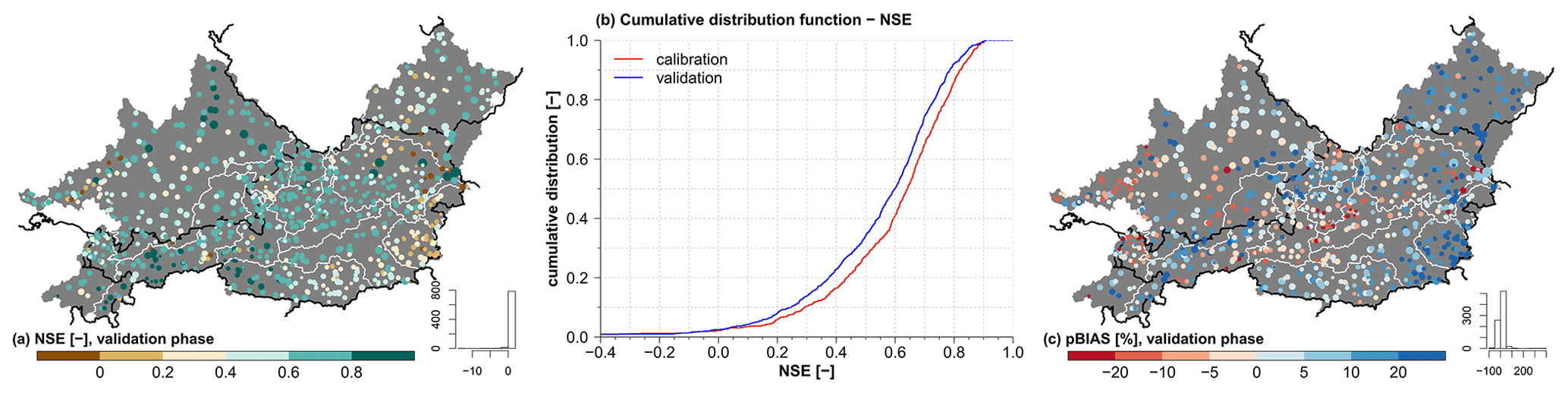
Figure 13 (a) Spatial distribution of NSE in validation phase. (b) Cumulative distribution of NSE in calibration and validation phase. (c) Spatial distribution of percent bias in validation phase (positive values indicate a simulated surplus). The size of the circles in plots (a) and (c) is proportional to the catchment area. © EuroGeographics for the administrative boundaries.

6.2 Model results

We evaluate the model results using standard performance metrics NSE (Eq. 2; Gupta and Kling, 2011; Jain and Sudheer, 2008; Knoben et al., 2019; McCuen et al., 2006; Nash and Sutcliffe, 1970; Schaefli and Gupta, 2007) and percentual (p) long-term bias (pBIAS, Eq. 3).

$$\begin{array}{}\text{(2)}& {\displaystyle }\text{NSE}=\mathrm{1}-{\displaystyle \frac{{\sum }_t^n{\left(Q_{\text{sim},t}-Q_{\text{obs},t}\right)}^{\mathrm{2}}}{{\sum }_t^n{\left(Q_{\text{obs},t}-\stackrel{\mathrm{‾}}{Q_{\text{obs}}}\right)}^{\mathrm{2}}}},\text{(3)}& {\displaystyle }\text{pBIAS}={\displaystyle \frac{\stackrel{\mathrm{‾}}{Q_{\text{sim}}}-\stackrel{\mathrm{‾}}{Q_{\text{obs}}}}{\stackrel{\mathrm{‾}}{Q_{\text{obs}}}}}\times \mathrm{100},\end{array}$$

where Q_sim represents the simulated and Q_obs the gauged runoff. The dash above the variable indicates the arithmetic mean.

The NSE ranges from −9.26 (calibration)$/-$13.96 (validation) to $\mathrm{0.91}/\mathrm{0.90}$ (Fig. 13b) with an area-unweighted median of $\mathrm{0.64}/\mathrm{0.60}$. Inadequate model performance (Fig. 13a) can mostly be explained by (i) cross-basin water transfers in karstified regions (see Fig. 11c), which are not accounted for in the model; (ii) a clear water surplus especially in eastern regions caused by overestimation in precipitation inputs or underestimation in evapotranspiration (Fig. 13c); or (iii) artificial structures, which were completed after the start of the calibration period (and thus were not specified in the artificial cross-basin water transfers). Rather good NSE values (>0.6) can be observed primarily at (i) gauges with large catchment areas (Fig. 13a), (ii) rainfall-dominated catchments (Fig. 6c) or (iii) gauges which are not too strongly influenced by large water reservoirs.

The overall area-unweighted median pBIAS (Fig. 13c) is +6.1 % in calibration and +4.4 % in the validation phase, which indicates either a precipitation surplus provided by ERA5-Land or underestimation of evapotranspiration. Herrnegger et al. (2012) show that the Thornthwaite approach tends to provide too-low PET sums in alpine regions. Although air temperature is an important driver of or proxy for evapotranspiration, other meteorological parameters, namely radiation, wind and relative humidity, are equally or probably more important factors. This is especially the case where lower air temperatures are present (especially in alpine regions) and other meteorological drivers of evapotranspiration, apart from temperature, become more important. The area-weighted mean of the PET-correction factor “ETSLPCOR” after calibration is 1.73 (with an upper boundary of 2.0; see Table C1), which indicates compensation for too-low PET values in the calibration procedure. Considering that the long-term evapotranspiration totals of the model output (“ETAsum” in the supplied shapefile Hyd_model.shp) seem quite plausible (e.g., compared to Fig. 20 in Herrnegger et al., 2012, or Map 3.3 in HAO, 2007), the reason for runoff surplus is likely a precipitation surplus in the ERA5-Land input. Klingler et al. (2020) show that CHIRPS Daily v2 (Funk et al., 2015) reflects long-term precipitation sums in the Mur catchment in the south of the Alps quite well. Figure 4e in contrast indicates that ERA5-Land in general provides considerably higher precipitation sums compared to CHIRPS Daily v2. This, in combination with our restriction to simulate somewhat realistic ETA fluxes, probably explains the many positive biases in the simulations of alpine catchments. The tight corset regarding ETA fluxes, in combination with too-high precipitation input, clearly leads to a lower model performance. Machine learning approaches, with few exceptions (e.g., Hoedt et al., 2021), ignore these physical constraints, and it is clear that higher model performance can be achieved when ignoring the mass balance or the realistic partitioning of precipitation in ETA and runoff.

Lastly, providing something like a disclaimer, it is important to stress that the simulation results stem from a large-scale model, which in this form has previously not been available. To our knowledge, no hydrological model existed which (i) covers such a large domain in Central Europe in such detail (∼170 000 km² in nine countries divided into 859 sub-basins), (ii) uses so many discharge observations for calibration and validation, and (iii) considers cross-basin water transfers. Although great care and love for detail was invested in the model setup of COSERO, it cannot be guaranteed that all local hydrometeorological features are represented, and room for improvement probably remains. Consequently, this baseline model may locally exhibit significant deviations from real-world hydrological conditions. This however generally remains a challenge for many large-scale hydrological models.

7 Data availability

LamaH is freely available at https://doi.org/10.5281/zenodo.4525244 (Klingler et al., 2021). The dataset is basically divided into seven parts including the basin delineation A, B and C; gauges; stream network; hydrological model; and appendix. The first four parts mentioned contain shapefiles and various text files regarding the attributes as well as time series. The stream network is available with shapefiles which contain numerous attributes. Various in- and outputs (e.g., parameter field, fluxes or evaluations) are provided for the hydrological model. The entire folder structure, supplement regarding the time series, and required references are in the folder “Info”. The runoff time series of the German federal states Bavaria and Baden-Württemberg are retrospectively checked and updated by the hydrographic services. Therefore, it might be appropriate to obtain more up-to-date runoff data from GKD (2020, https://www.gkd.bayern.de/en/rivers/discharge/tables, last access: 15 September 2020) or LUBW (2020, http://udo.lubw.baden-wuerttemberg.de/public/p/pegel_messwerte_leer, last access: 4 September 2020). Please consider also the disclaimer stated at Zenodo.

8 Code availability

We have used R codes from Nans Addor (Addor, 2017, https://github.com/naddor/camels, last access: 2 March 2020) for reproducing the climatic (Table A4) and hydrological (Table A5) indices as well as for creating Figs. 3, 5–13a and 13c. The color schemes in the plots are often based on ColorBrewer 2.0 (Brewer, 2021; https://github.com/axismaps/colorbrewer/, last access: 31 August 2021). Further relevant R and Python scripts for reproducing the dataset are available in the folder “G_appendix”.

9 Required additional references when using LamaH

We ask kindly for compliance in citing the following references when using LamaH, as an agreement to cite was usually a condition of sharing the data: BAFU (2020), CHMI (2020), GKD (2020), HZB (2020), LUBW (2020), BMLFUW (2013), Broxton et al. (2014), CORINE (2012), EEA (2019), ESDB (2004), Farr et al. (2007), Friedl and Sulla-Menashe (2019), Gleeson et al. (2014), HAO (2007), Hartmann and Moosdorf (2012), Hiederer (2013a, b), Linke et al. (2019), Muñoz Sabater et al. (2021), Muñoz Sabater (2019a), Myneni et al. (2015), Pelletier et al. (2016), Toth et al. (2017), Trabucco and Zomer (2019), and Vermote (2015).

10 Summary and conclusions

Hydrological studies often require an extensive foundation of data. In large-scale or cross-national projects, it is therefore often laborious and time-consuming to collect the required data and then to homogenize the usually different formats, definitions and conventions. Reasons are for instance the different organizational forms of the hydrographic authorities or communication barriers. LamaH provides a unique, homogeneous database for hydrological and other environmental sciences that can overcome the mentioned barriers. Apart from the complete territory of Austria, LamaH includes all neighboring upstream areas of the rivers flowing through Austria as well. LamaH contains runoff time series as well as 15 meteorological time series (daily and hourly resolution) and over 60 attributes for 859 catchments. Additionally, simulations from a conceptual hydrological model provide a baseline for further investigations. Three basin delineations allow investigations with individual catchments (as known from CAMELS) as well as within an interconnected river network considering intermediate catchments. It is clear that LamaH contains deficits and uncertainties due to the large number of data sources included. We however tried to consider and discuss most of these limitations.

Blöschl et al. (2019b) have highlighted numerous open hydrological challenges, such as runoff prediction in ungauged basins (PUB). Methods based on machine learning show promising results for time series prediction (e.g., Kratzert et al., 2019a, b, 2018). However, uniformly structured large-sample datasets are helpful when applying these data-driven methods because on the one hand the necessary preparatory work is drastically reduced and on the other hand the exchange or comparability of the modeling results is considerably facilitated. Given the scope of LamaH, we hope that this dataset will serve as a solid database for further investigations in various fields of hydrology and adjacent fields of environmental science. The high variability in the data in combination with the interconnected river network as well as the high temporal resolution of the time series could grant an improved understanding of processes in water transfer and storage if appropriate methods are used.

Appendix A

Table A1 Gauge referred attributes.

^a List of abbreviations for attribute fedstate: Austria (BLD – Burgenland, CRN – Carinthia, LAT – Lower Austria, SBG – Salzburg, STY – Styria, TYR – Tyrol, UAT – Upper Austria, VBG – Vorarlberg, VIE – Vienna), Germany (BAV – Bavaria, BWT – Baden-Württemberg), Switzerland (GRI – Grisons, STG – St Gallen), Liechtenstein (LIE – Liechtenstein), the Czech Republic (OLM – Olomouc, SBO – South Bohemian, SMO – South Moravian, VYS – Vysočina, ZLN – Zlín). ^b List of abbreviations for attribute region: 1 – Rhine, 2 – Danube above Inn, 3 – Inn above Salzach, 4 – Salzach, 5 – Inn under Salzach, 6 – Danube between Inn and Traun, 7 – Traun, 8 – Danube between Traun and Enns, 9 – Enns, 10 – Danube between Enns and Morava, 11 – Vltava, 12 – Morava, 13 – Danube between Morava and Leitha, 14 – Leitha, 15 – Rabnitz, 16 – Raab, 17 – Mur, 18 – Drava. ^c Only for basin delineation B and C. ^d Only for basin delineation A. ^e Visible in daily and hourly runoff time series. ^f End of the river segment (to which the attributes within the river network refer) can sometimes be rather far from the gauge. If a single river segment extended over several gauges, the ID of the river segment was only indicated at the most downstream gauge.

Table A2 Meteorological variables from ERA5-Land dataset (Muñoz Sabater, 2019a).

Table A3 Topographic indices.

^* Upscaling approach 2.

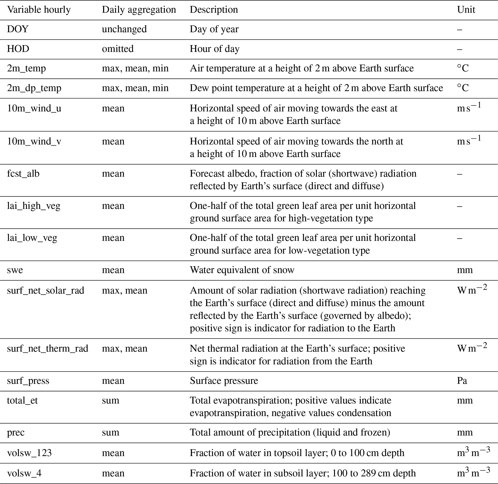
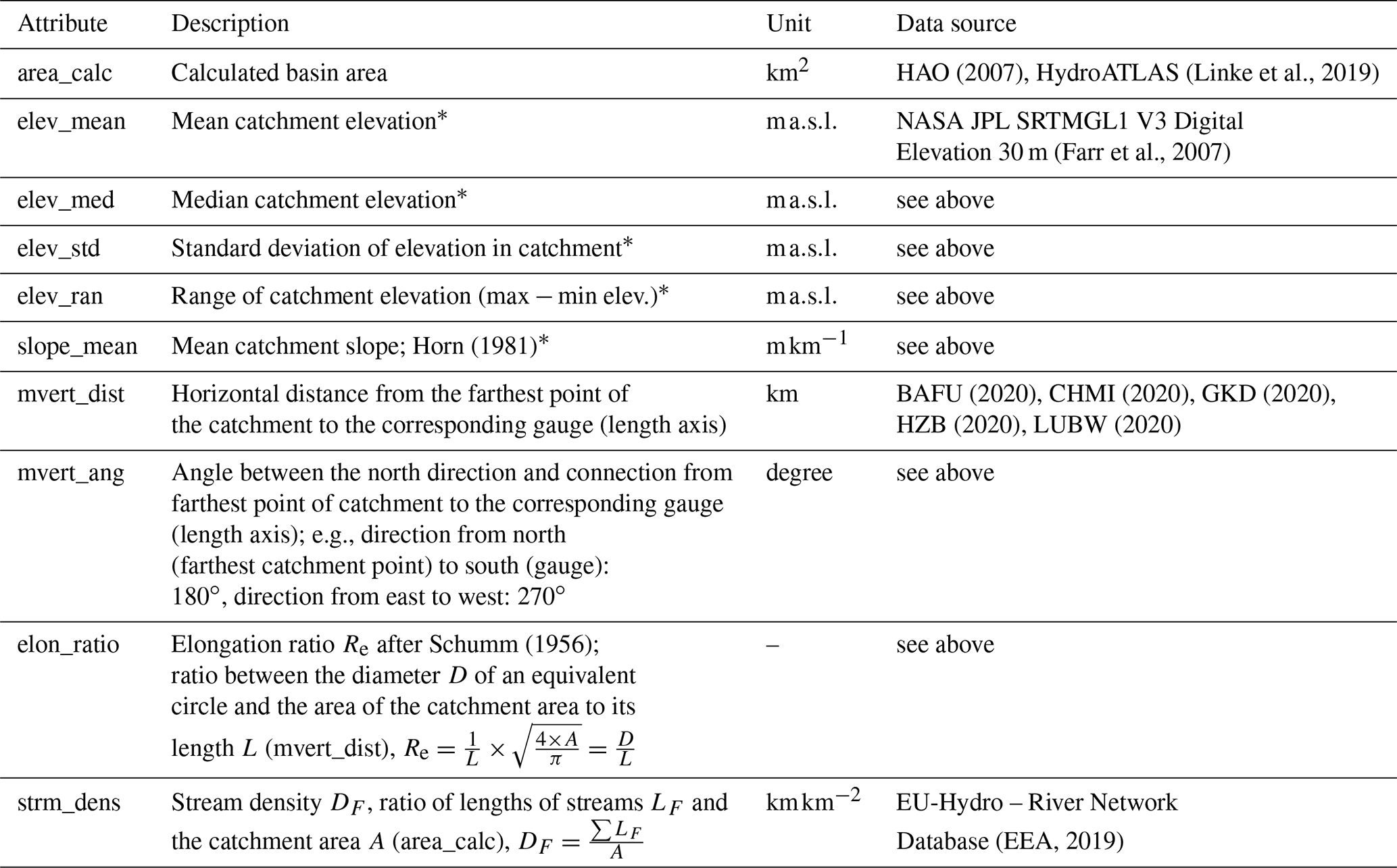
Table A4 Climatic indices.

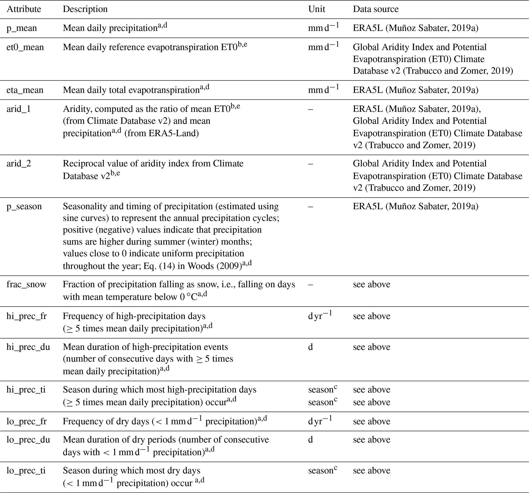
^a Period 1 October 1989 to 30 September 2009. ^b Period 1970 to 2000. ^c List of abbreviations for seasons: djf – December–January–February, mam – March–April–May, jja – June–July–August, son – September–October–November. ^d Upscaling approach 1. ^e Upscaling approach 2.

Table A5 Hydrological signatures.

^a Period 1 October 1989 to 30 September 2009 and additionally from the first 1 October in the time series after 1981 to 30 September 2017. ^b Upscaling approach 1. ^c No values if there are more than 5 % gaps in the calculation period. ^d No values for basins/gauges which are attributed with degimpact = x.

Table A6 Land cover characteristics.

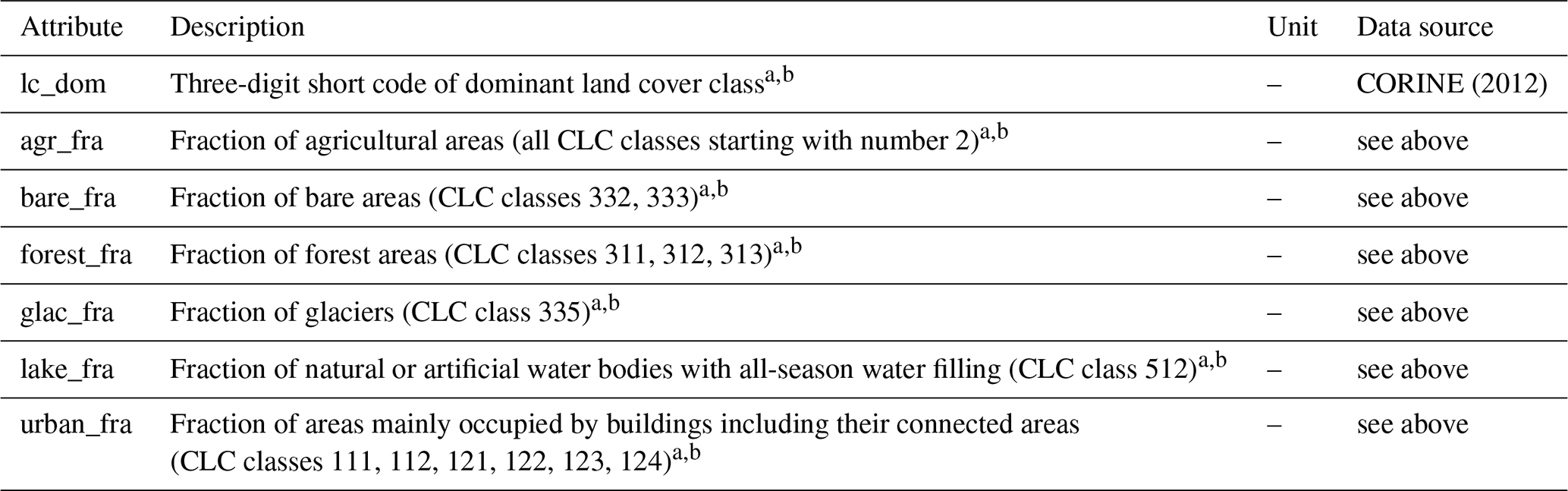
^a Upscaling approach 2. ^b Land class nomenclature is listed in the folder G_appendix.

Table A7 Vegetation indices.

^* Upscaling approach 2.

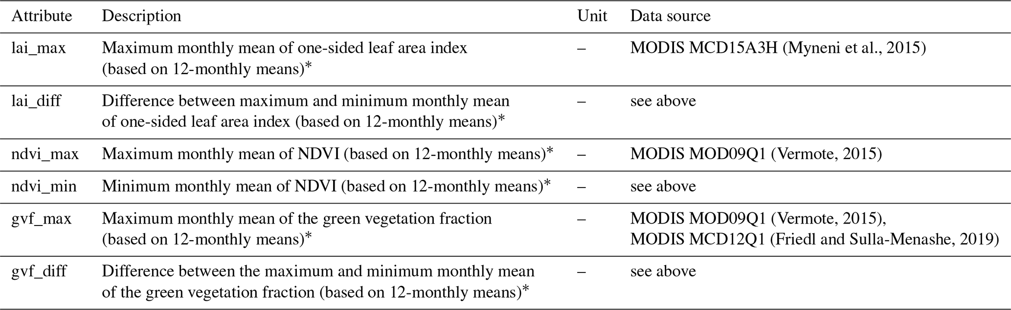
Table A8 Soil characteristics.

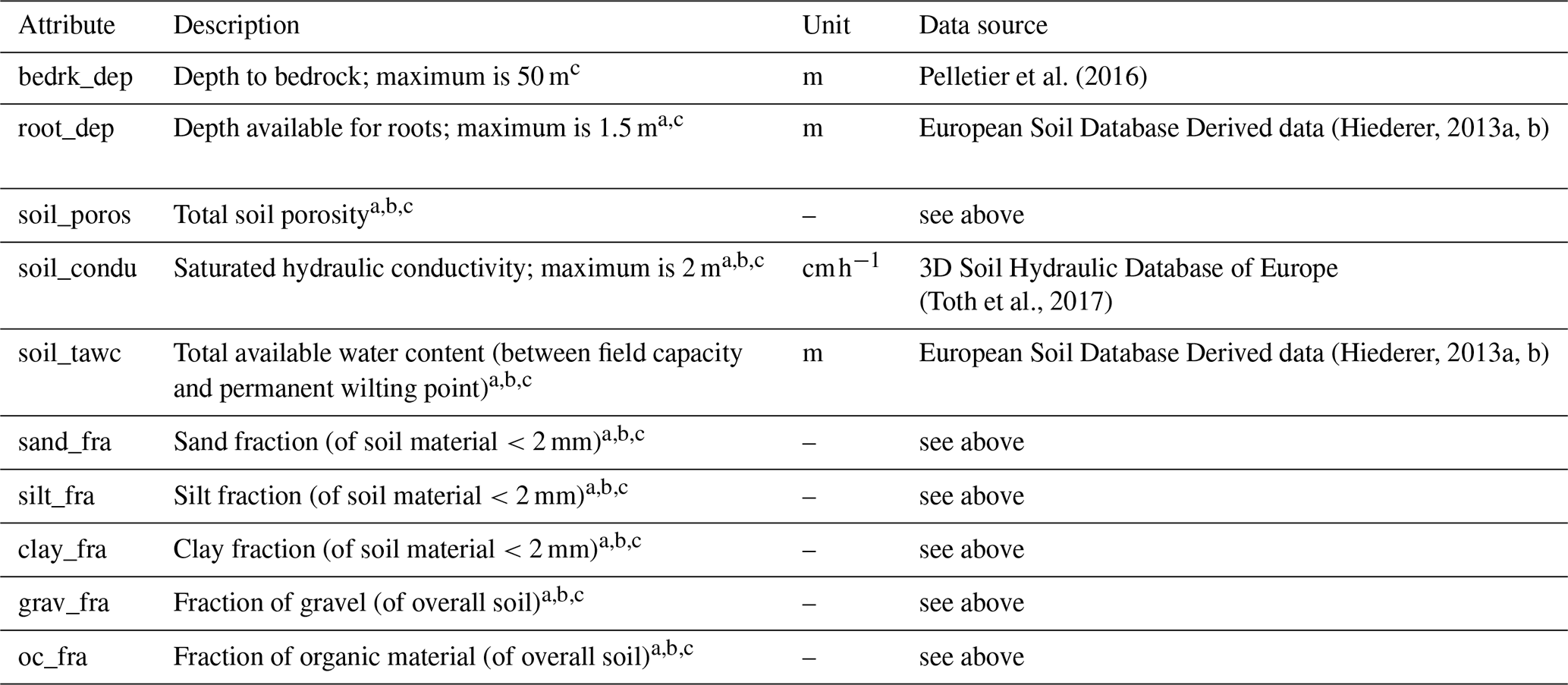
^a Areas marked as water or bedrock were excluded from calculation. ^b Aggregation weighted by depth over the different soil layers. ^c Upscaling approach 2.

Table A9 Geological attributes.

^a Upscaling approach 1. ^b Upscaling approach 2.

Table A10 Attributes in the accompanying file Water_balance.csv.^e

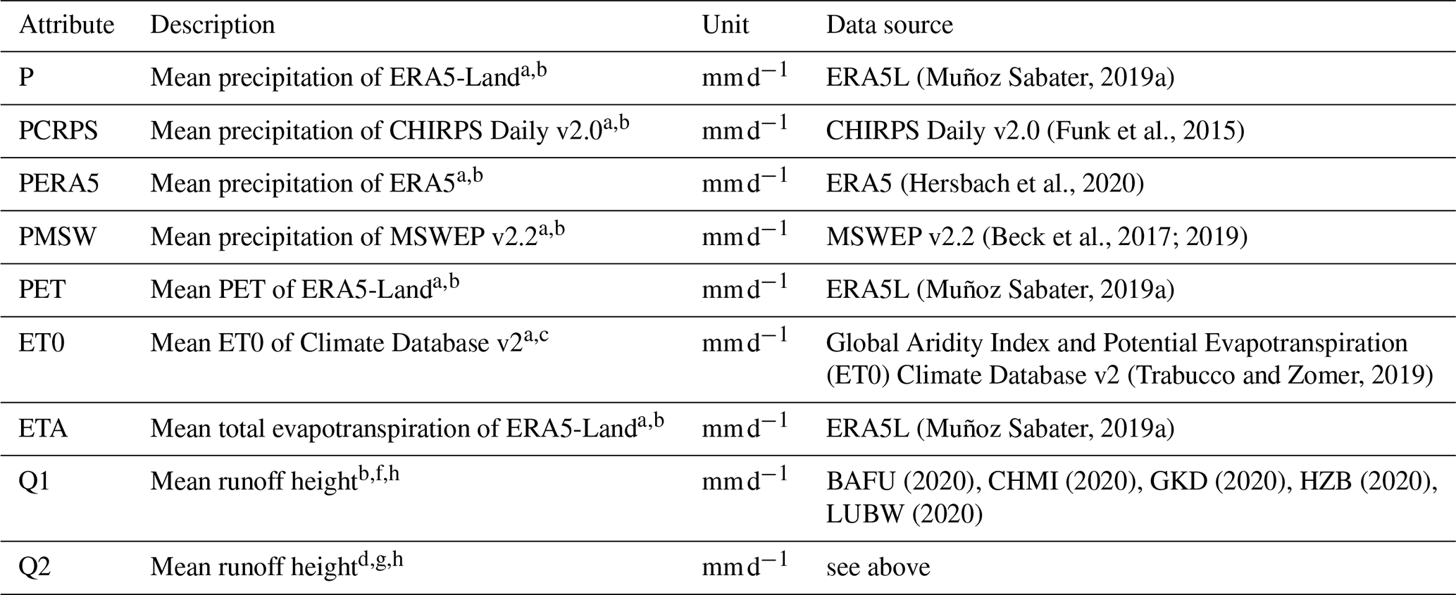
^a Computed for basin delineation A. ^b Period 1 October 1989 to 30 September 2009. ^c Period 1970 to 2000. ^d Period from the first 1 October in the time series after 1981 to 30 September 2017. ^e No values where corresponding gauge is attributed with degimpact = x (Table 1). ^f No values for gauges whose time series do not cover the full period. ^g Values only if at least 5 years of observations is available. ^h No values if there are more than 5 % gaps in the calculation period.

Table A11 Attributes in the accompanying file Crossbasin_water_transfers.csv.^*

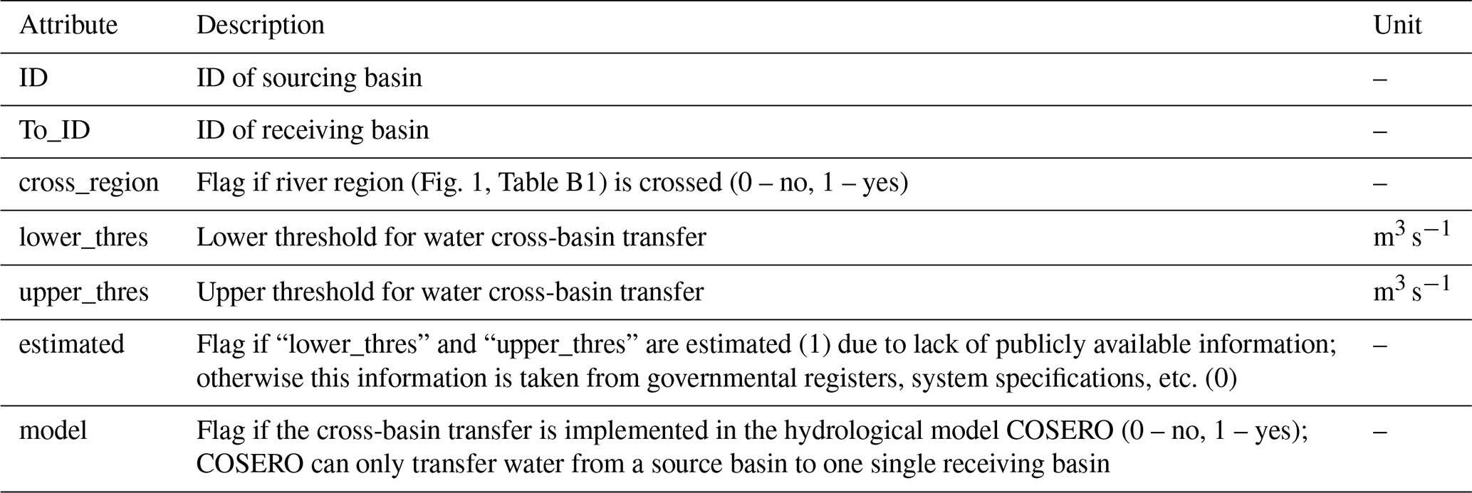
^* Derived for basin delineation B.

Appendix B

Table B1 Overview of the river regions.

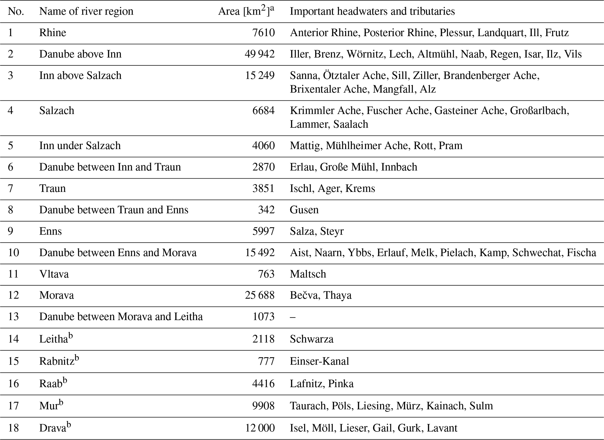
^a Area which is covered by basin delineation B. ^b River joins the Danube outside the project area in Hungary/Croatia.

Appendix C

Table C1 Calibrated parameters in the hydrological model COSERO.

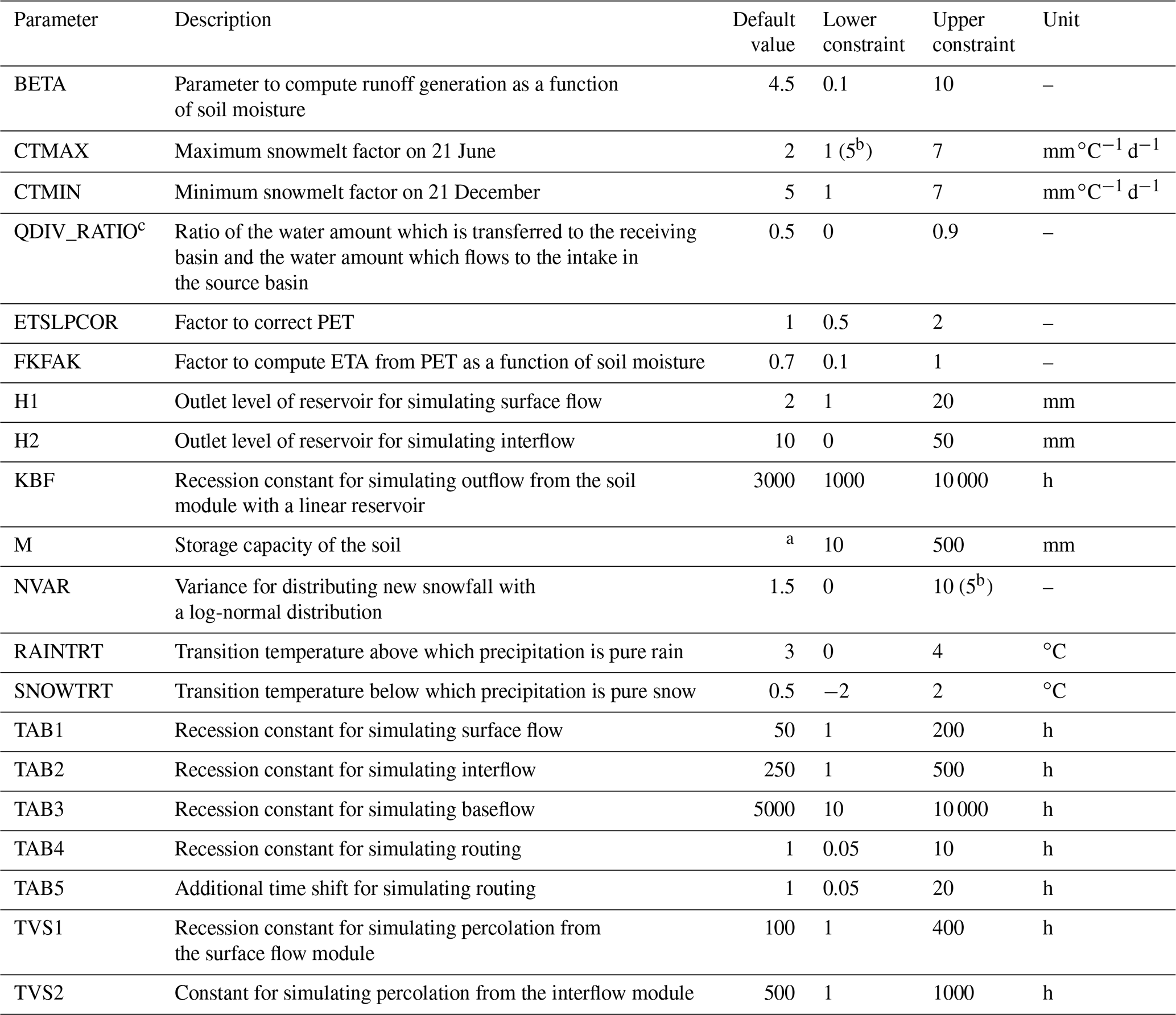
^a Parameter soil_tawc (Table A8). ^b For basins with a mean catchment elevation (elev_mean in Table A3) of at least 2000 $\mathrm{m}\mathrm{a}.\mathrm{s}.\mathrm{l}.$ ^c Calibrated only if there is a cross-basin water transfer (see file Crossbasin_water_transfers.csv, Table A11); otherwise parameter is set to 0.

Table C2 Provided input/output time series from the hydrological model COSERO.

^a Suffix _A indicates that aggregation was performed for basin delineation A (full upstream topographic catchment area), while suffix _B indicates aggregation for basin delineation B (intermediate catchments). ^b Set to −999 if basin was calibrated together with the next downstream basin due to no or too few runoff observations in the calibration period.