the Creative Commons Attribution 4.0 License.
the Creative Commons Attribution 4.0 License.
 | 16 Feb 2021
Synthesis of global actual evapotranspiration from 1982 to 2019
Abdelrazek Elnashar
Linjiang Wang
Bingfang Wu
Weiwei Zhu
Hongwei Zeng
As a linkage among water, energy, and carbon cycles, global actual evapotranspiration (ET) plays an essential role in agriculture, water resource management, and climate change. Although it is difficult to estimate ET over a large scale and for a long time, there are several global ET datasets available with uncertainty associated with various assumptions regarding their algorithms, parameters, and inputs. In this study, we propose a long-term synthesized ET product at a kilometer spatial resolution and monthly temporal resolution from 1982 to 2019. Through a site-pixel evaluation of 12 global ET products over different time periods, land surface types, and conditions, the high-performing products were selected for the synthesis of the new dataset using a high-quality flux eddy covariance (EC) covering the entire globe. According to the study results, Penman–Monteith–Leuning (PML), the operational Simplified Surface Energy Balance (SSEBop), the Moderate Resolution Imaging Spectroradiometer (MODIS, MOD16A2105), and the Numerical Terradynamic Simulation Group (NTSG) ET products were chosen to create the synthesized ET set. The proposed product agreed well with flux EC ET over most of the all comparison levels, with a maximum relative mean error (RME) of 13.94 mm (17.13 %) and a maximum relative root mean square error (RRMSE) of 38.61 mm (47.45 %). Furthermore, the product performed better than local ET products over China, the United States, and the African continent and presented an ET estimation across all land cover classes. While no product can perform best in all cases, the proposed ET can be used without looking at other datasets and performing further assessments. Data are available on the Harvard Dataverse public repository through the following Digital Object Identifier (DOI): https://doi.org/10.7910/DVN/ZGOUED (Elnashar et al., 2020), as well as on the Google Earth Engine (GEE) application through this link: https://elnashar.users.earthengine.app/view/synthesizedet (last access: 21 January 2021).
- Article
(21903 KB) - Full-text XML
- BibTeX
- EndNote


Over most of the global land area, terrestrial evapotranspiration (ET) considers the second largest element of the hydrological cycle after precipitation (Waring and Running, 2007b; Bastiaanssen et al., 2014) and represents the linkage between water, energy, and carbon cycles (Gentine et al., 2019; Yang et al., 2016; Ferguson and Veizer, 2007) and ecosystem services (Almusaed, 2011; Yang et al., 2015; Revelli and Porporato, 2018).
Hence, the accurate estimation of global ET is essential for understanding the global hydrological cycle and water budgets (Oki and Kanae, 2006; Trenberth et al., 2007; Rodell et al., 2015), global drought (Sheffield et al., 2012; Naumann et al., 2018; Spinoni et al., 2019; Lu et al., 2019; Forootan et al., 2019), impacts of climate change (Waring and Running, 2007a; Zomer et al., 2008; Scheff and Frierson, 2014; Pan et al., 2015), climate change and global water resources (Arnell, 1999; Haddeland et al., 2014; Arnell and Lloyd-Hughes, 2014), global transboundary basin water scarcity (Degefu et al., 2018), water competition within a basin (Scott et al., 2001), and water stress/conflict within transboundary basins (Samaranayake et al., 2016; Munia et al., 2016; Bastiaanssen et al., 2014).
While precipitation and runoff, which are other paramount factors of the global water balance, can be directly measured by in situ weather stations and stream gauge networks, as well as the availability of several datasets of remotely sensed precipitation (Funk et al., 2015; Ashouri et al., 2015; Huffman et al., 1997; Yamamoto and Shige, 2015), it is difficult to measure ET, especially at large spatial scales (Senay et al., 2012; Zhang et al., 2016).
Recently, several global ET datasets have become available for a variety of purposes, and they have been generated using remote sensing models, land surface models (LSMs), and hydrological models (Trambauer et al., 2014; Li et al., 2018; Sörensson and Ruscica, 2018). There are many differences among these models concerning their algorithms, parameters, and inputs, and they produce different levels of uncertainty (Wang and Dickinson, 2012; Xu et al., 2019; Weerasinghe et al., 2020; Vinukollu et al., 2011a). The remote sensing model, which mainly focuses on thermal remote sensing and the energy balance equation, will be represented by MOD16A2 (Mu et al., 2011), Penman–Monteith–Leuning (PML; Zhang et al., 2019), the operational Simplified Surface Energy Balance (SSEBop; Senay et al., 2013), the Surface Energy Balance System (SEBS; Chen et al., 2013), the Numerical Terradynamic Simulation Group (NTSG; Zhang et al., 2010), and the Global Land Evaporation Amsterdam Model (GLEAM) v3.3b (Miralles et al., 2011b). The land surface model uses quantitative methods to simulate the vertical exchanges of water and energy fluxes between the atmosphere and the land surface, as represented by the Global Land Data Assimilation System (GLDAS) ET (Rodell et al., 2004), GLEAM v3.3a (Miralles et al., 2011b), and the Famine Early Warning Systems Network (FEWS NET) Land Data Assimilation System (FLDAS) (McNally et al., 2017). TerraClimate, which is a hydrological model, is based on a one-dimensional water balance approach (Abatzoglou et al., 2018). However, the availability of many datasets introduces challenges related to how users choose the appropriate dataset for their purposes (Wu et al., 2020).
Some studies have evaluated global ET products using an inferred estimate of ET obtained by subtracting discharge (Q) from precipitation (P), ET = P−Q, over global river basins (Zhang et al., 2010; Vinukollu et al., 2011a, b), continental river basins (Weerasinghe et al., 2020), transboundary river basins (Hofste, 2014), and national river basins (Zhong et al., 2020). Some, on the other hand, have used the ensemble ET product as observed data for evaluating certain ET products (Hofste, 2014; Trambauer et al., 2014; Andam-Akorful et al., 2015; Bhattarai et al., 2019).
Although flux eddy covariance (EC) ET is commonly flawed, particularly concerning energy balance closure at some sites (Foken, 2008; Helgason and Pomeroy, 2012), relatively short periods, and sparse spatial coverage, it is the most direct method for measuring the exchange between the surface and the atmosphere in different ecosystems (Foken et al., 2012; Baldocchi, 2014). Thus, site-pixel-level validation of certain ET products against flux EC ET as typically observed data has been performed by several studies in specific regions, e.g., globally (Leuning et al., 2008; Zhang et al., 2010; Ershadi et al., 2014; Michel et al., 2016), Asia (Kim et al., 2012), South Africa (Majozi et al., 2017), Europe (Ghilain et al., 2011; Hu et al., 2015), North America (Jiménez et al., 2009; Mu et al., 2011), Europe and the United States (Miralles et al., 2011b), the United States (Vinukollu et al., 2011b; Velpuri et al., 2013; Xu et al., 2019), and China (Jia et al., 2012; Liu et al., 2013; Y. Chen et al., 2014; Tang et al., 2015; Yang et al., 2017; Li et al., 2018). Few previous studies have focused on merging certain ET products to create an ensemble ET product. For instance, Vinukollu et al. (2011a), Mueller et al. (2013), and Badgley et al. (2015) used all ET products and created a merged product with a low spatial resolution. There are some global merged benchmarking evapotranspiration products. Vinukollu et al. (2011a) generated an ensemble of six global ET datasets at a daily timescale and 0.5∘ × 0.5∘ (≈55 km) spatial resolution for the period 1984–2007 using two surface radiation budget products and three models (i.e., surface energy balance, revised Penman–Monteith, and modified Priestley–Taylor). They reported that the ensemble simple mean value was reasonable; however, it was generally highly biased globally. Mueller et al. (2013) presented two monthly global ET products that differed in their input ET members and temporal coverage. The first dataset consisted of 40 datasets for the period 1989–1995, while the second dataset merged 14 datasets from 1989 to 2005. Their ET was derived from satellite and/or in situ observations (diagnostic) or calculated via LSMs driven with observation-based forcing or output from atmospheric reanalysis. Hence, they provided four merged synthesis products, one including all datasets and three including datasets of each category (i.e., diagnostic, LSM, and reanalysis). They introduced the first benchmark products for global ET and found that its multiannual variations showed realistic responses and were consistent with previous findings. Badgley et al. (2015) used a Priestley–Taylor Jet Propulsion Lab (PT-JPL) model with 19 different combinations of forcing data to produce global ET estimates from 1984 to 2006 at a 1∘ × 1∘ (≈100 km) spatial resolution. The ensemble ET members changed according to the number of products available each year, which ranged between 4 and 12 members for 1999/2000 and 2001/2002, respectively. Their study focused on the uncertainty in global ET estimates resulting from each class of input forcing datasets.
However, from the aforementioned studies, we can report three findings: (1) no single ET product performed better than any other over different land surface types and conditions, (2) no one product generated a single dataset for users, and (3) the created ensemble ET products relied on several individual ET products and were not based on the product with the best performance.
From our point of view, this work attempts to add to the growing scientific literature by using a high-quality dataset from global flux towers for further validations and intercomparison between different global ET products to understand their behavior within defined land cover types, elevation levels, and climatic classes. Moreover, we attempt to build an ensemble ET product that has a minimum level of uncertainty over as many conditions as possible. The study has two objectives: (1) to assess global ET products with in situ data derived from global flux towers across a variety of land surface types and conditions to gain a better understanding of the disparities among datasets and (2) to synthesize an ensemble global ET product with minimum uncertainties over more land surface types, climate systems, and monthly, annually, and interannual time steps for a longer time.
2.1 Evapotranspiration
A total of 12 global ET datasets were explored in the current study (Table 1 and Appendix A). Of them, five datasets used the Moderate Resolution Imaging Spectroradiometer (MODIS) as input, including two versions (V6 and V105) of the Global Evapotranspiration Project (MOD16A2), the Penman–Monteith–Leuning ET (PML), the operational Simplified Surface Energy Balance ET (SSEBop), and the Surface Energy Balance System (SEBS). One dataset used the Advanced Very High-Resolution Radiometer (AVHRR) as input, including the Numerical Terradynamic Simulation Group (NTSG). The remainder mainly used meteorological datasets as direct input, including field measurements such as TerraClimate and reanalysis datasets such as FLDAS and GLDAS. The algorithm used in 12 global ET datasets is mainly the Penman–Monteith model, except for FLDAS and GLDAS, which use the LSM, and TerraClimate, which uses the soil water balance model. Priestley–Taylor is used to estimate evaporation from open water by NTSG, while Penman evapotranspiration is used in PML for water body, snow, and ice evaporation. SSEBop, SEBS, NTSG, and GLEAM are individually managed, and other ET products, as well as elevation data, are available from GEE.
Table 1Global ET products.
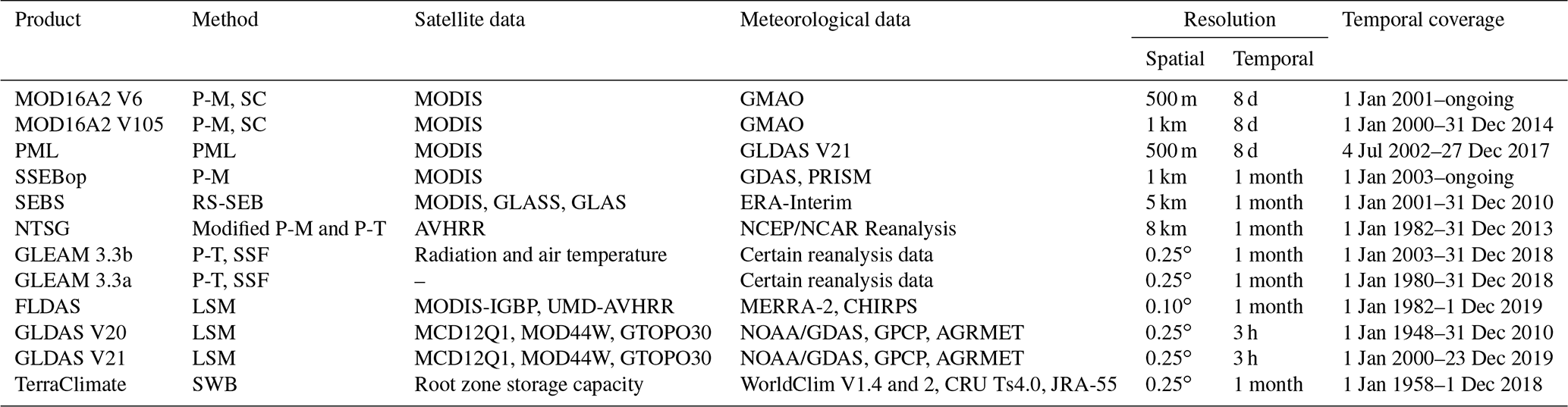
Note: P-M: Penman–Monteith; PML: Penman–Monteith–Leuning; SC: surface conductance; P-T: Priestley–Taylor; RS-SEB: remotely sensed surface energy balance; LSM: land surface model; SSF: soil stress factor; SWB: soil water balance; GMAO: Global Modelling and Assimilation Office for daily meteorological reanalysis data; GDAS: Global Data Assimilation System; PRISM: Parameter-elevation Regressions on Independent Slopes Model; GLASS: Global Land Surface Satellite; GLAS: Geoscience Laser Altimeter System; MERRA-2: Modern-Era Retrospective analysis for Research and Applications version 2; CHIRPS: Climate Hazards Group InfraRed Precipitation with Station data; RFE2: the African Rainfall Estimation version 2.0; NOAA: National Oceanic and Atmospheric Administration; GPCP: Global Precipitation Climatology Project; AGRMET: Agricultural Meteorological modeling system; CRU Ts4.0: Climate Research Unit time series data version 4.0; JRA-55: Japanese 55-year Reanalysis.
Table 2Regional ET products.
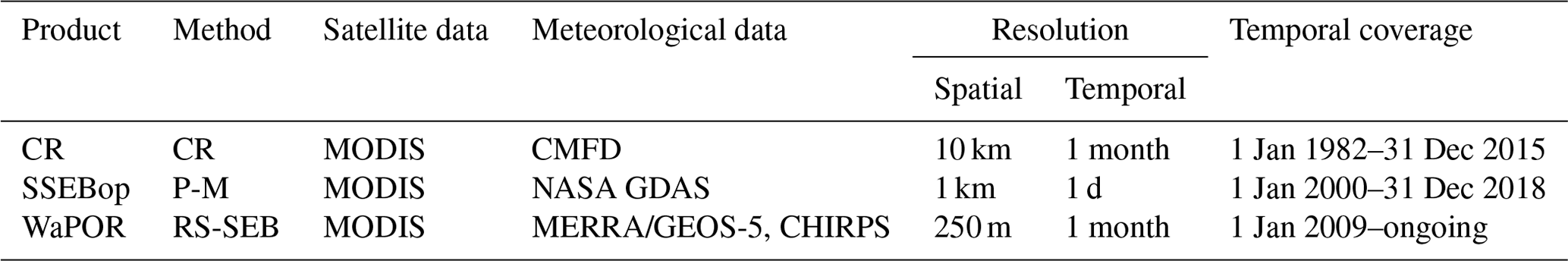
Note: CR: complementary relationship; P-M: Penman–Monteith; P-T: Priestley–Taylor; RS-SEB: remotely sensed surface energy balance; CMFD: China Meteorological Forcing Dataset; NASA GDAS: National Oceanic and Atmospheric Administration's (NOAA) Global Data Assimilation System; MERRA: Modern-Era Retrospective Analysis for Research and Applications; GEOS-5: Goddard Earth Observing System, version 5; CHIRPS: Climate Hazards Group InfraRed Precipitation with Stations.
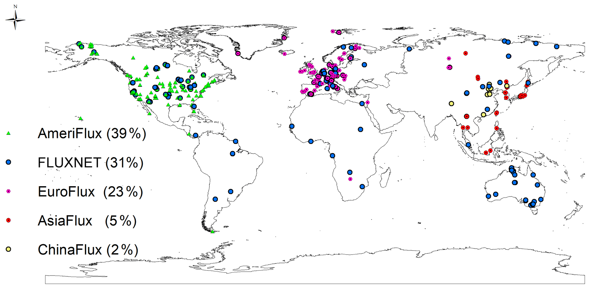
Figure 1Spatial distribution of 645 in situ flux EC sites across the world.
Three regional ET datasets were used for the comparison of consistent agreement over China, the United States, and the African continent (Table 2). Over mainland China, the complementary relationship (CR) ET product was used (Ma et al., 2019); it is estimated monthly at a 0.1∘ (≈10 km) spatial resolution over 1982–2015 and can be retrieved from http://en.tpedatabase.cn (last access: 21 January 2021). For the United States, daily SSEBop was used (Savoca et al., 2013; Senay and Kagone, 2019). These data are produced at a 0.009∘ × 0.009∘ (≈1 km) grid cell spatial resolution from 2000 to 2018 and can be downloaded from https://earlywarning.usgs.gov/ssebop/modis/daily (last access: 21 January 2021). Daily SSEBop is aggregated to monthly time steps to be comparable with the synthesized ET temporal resolution. The Food and Agriculture Organization (FAO) Water Productivity through Open access of Remotely sensed derived ET product (FAO WaPOR version 2) was used for Africa (FAO, 2018, 2020). These data estimates are the sum of ET and interception, provided at a 0.002∘ × 0.002∘ (≈250 m) spatial resolution with a monthly temporal resolution from 2009. WaPOR ET estimates are available through the following website: https://wapor.apps.fao.org/home/WAPOR_2/1 (last access: 21 January 2021).
2.2 Flux EC data
Comprehensive flux EC ET data from 645 sites (Fig. 1 and Table 3) – AmeriFlux, FLUXNET, EuroFlux, AsiaFlux, and ChinaFlux – were collected and processed to examine the performance of different estimated ET products. The downloaded EC data are half-hourly text-type data, while the periods of flux EC ET ranged from 1 year (12 months) to 21 years (252 months) from 1994 to 2019. The gap-filling technique was applied to the downloaded in situ EC data (Reichstein et al., 2005). Different EC flux sites were spatially distributed on the heterogeneous underlying surface corresponding to different land cover types according to the International Geosphere–Biosphere Programme (IGBP) classification system, which is recorded in each flux attribute data. The in situ measured ET (mm d−1) can be obtained by the half-hourly average latent heat flux (LE, W m−2 s−1) through Eq. (1) (Su, 2002):
where (W m−2 s−1) is the daily average of the half-hourly average latent heat flux, and λ is the latent heat of evaporation. λ varies with air temperature in hydrologic or agricultural system modeling but only to a small extent (Walter et al., 2001), and the value acts directly on the accuracy of the estimated in situ measured ET. Considering that there are very limited impacts of the changes in air temperature on the estimated in situ measured ET (Henderson-Sellers, 1984; Li et al., 2018), the constant value of 2.45 MJ kg−1 is fixed in the calculation above (Walter et al., 2001).
Table 3Summary of 645 in situ EC flux sites.

Note: ENF: evergreen needleleaf forest; EBF: evergreen broadleaf forest; DNF: deciduous needleleaf forest; DBF: deciduous broadleaf forest; MF: mixed forest; CSH: closed shrubland; OSH: open shrubland; WSA: woody savanna; SAV: savanna; GRA: grassland; WET: permanent wetland; CRO; cropland; URB: urban and buildup land; SNO: permanent snow and ice; BSV: barren or sparsely vegetated area; WAT: water body.
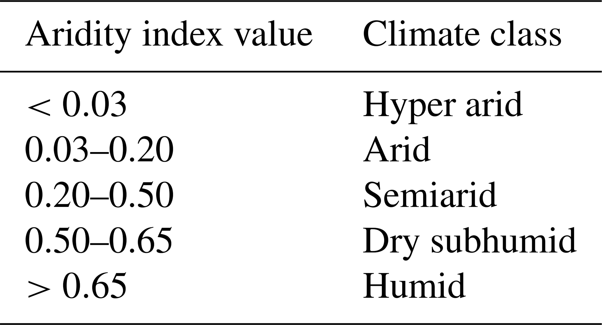
2.3 Aridity index
The mean global aridity index dataset was produced by Zomer et al. (2008) using WorldClim global climate data. The aridity index was estimated as the mean annual precipitation divided by the mean annual potential evapotranspiration, and the latter was calculated by the Hargreaves equation. The spatial resolution was 0.0083∘ × 0.0083∘ (≈1 km) grid cells (Trabucco and Zomer, 2018), and the data can be downloaded from the following website: https://cgiarcsi.community/data/global-aridity-and-pet-database (last access: 21 January 2021).
Table 4Climate classification according to the global aridity index values.
2.4 Elevation data
The Shuttle Radar Topography Mission (SRTM) data were provided at a resolution of 1 arcsec and void-filled (Farr et al., 2007). For the geographic areas outside the SRTM coverage area, the Global Multi-resolution Terrain Elevation Data 2010 (GMTED2010), which have a resolution of 7.5 arcsec, were used (Danielson and Gesch, 2011).

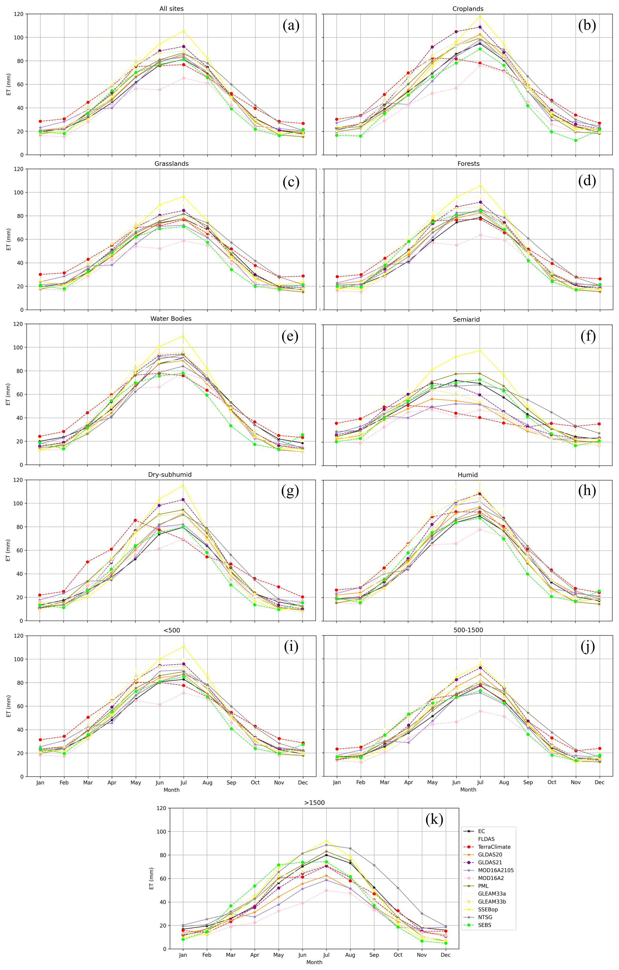
Figure 3Monthly average flux EC ET and 12 ET products over all flux sites (a), land cover types (croplands: b; grasslands: c; forests: d; water bodies: e), climate classes (semiarid: f; dry subhumid: g; humid: h), and elevation levels (<500 m: i; 500–1500 m: j; >1500 m: k).
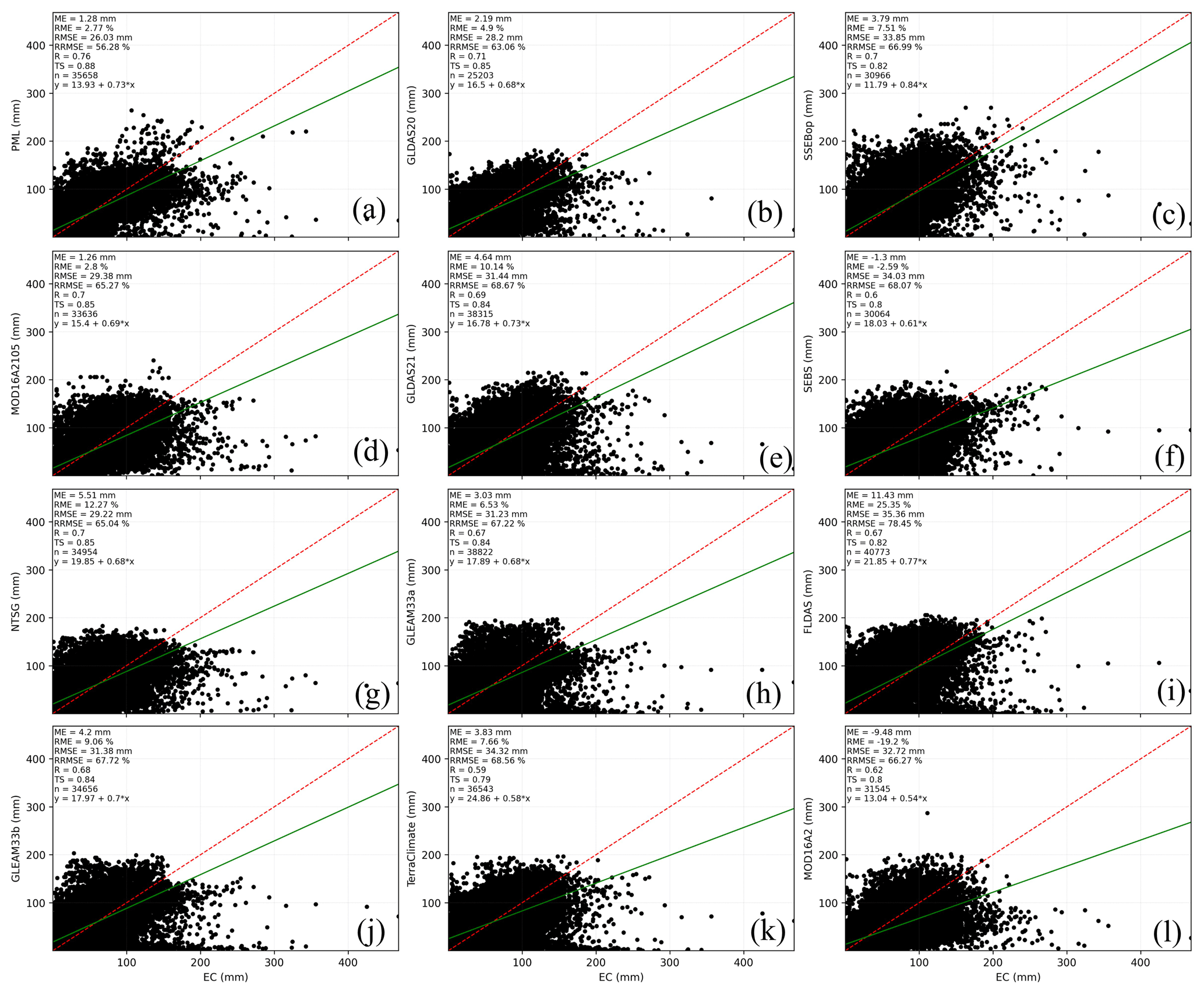
Figure 4Monthly ET products (PML: a; GLDAS20: b; SSEBop: c; MOD16A2105: d; GLDAS21: e; SEBS: f; NTSG: g; GLEAM33a: h; FLDAS: i; GLEAM33b: j; TerraClimate: k; MOD16A2: l) against flux EC ET aggregated for all sites.
3.1 Assessment
Because ET is highly variable in both space and time (Schaffrath and Bernhofer, 2013; Fisher et al., 2017), a comprehensive evaluation from different perspectives is required (Trambauer et al., 2014; McCabe et al., 2016; Li et al., 2018). For each flux tower location, the aridity index, elevation, and estimated ET data were extracted. The aridity index was classified (Table 4) according to the United Nations Environment Programme definition (UNEP, 1997) into four classes, i.e., humid: 361 (56 %), semiarid: 167 (26 %), dry subhumid: 82 (13 %), and arid: 35 (5 %). Elevations were classified into three levels, i.e., <500 m: 452 (70 %), 500–1500 m: 135 (21 %), and >1500 m: 58 (9 %). Land cover included five types, i.e., forests: 349 (54 %), grasslands: 128 (20 %), croplands: 89 (14 %), water bodies: 73 (11 %), and others (barren land and permanent snow and ice): 6 (1 %). Accordingly, the following metrics were estimated using Eqs. (2)–(7):
where ME is the mean error, RME is the relative mean error, RMSE is the root mean square error, RRMSE is the relative root mean square error, R is the correlation coefficient, TS is the Taylor score, n is the sample number, i is the ith sample, X is the mean of the observed EC ET data, Y is the mean of different estimated ET data, SD is the standard deviation of the estimated ET normalized by the standard deviation of the observed EC ET, and R0 is the maximum theoretical R, with an R0 value of 0.9976 (Taylor, 2001).
The magnitude of ME (the absolute value) is used as a bias indicator (Mu et al., 2011; Yang et al., 2017), while its sign indicates whether different ET products overestimate or underestimate the flux EC ET values. The accuracy of each ET product can be described by the RMSE (Miralles et al., 2011b; Hu et al., 2015). Moreover, the relative values of ME and RMSE are used for a fairer comparison between certain ET products among different regions and periods (Majozi et al., 2017). In addition, correlation coefficients (R values) are used to measure the strength of the relation between flux EC ET and different ET products (Ghilain et al., 2011; Hu et al., 2015), and with the aid of the Taylor score (TS), the overall performance of each product can be described well (Taylor, 2001; Mu et al., 2011). To rank each ET product, the lower ME, RME, RMSE, and RRMSE values and the higher R and TS values are desired (lower biases and higher accuracies).
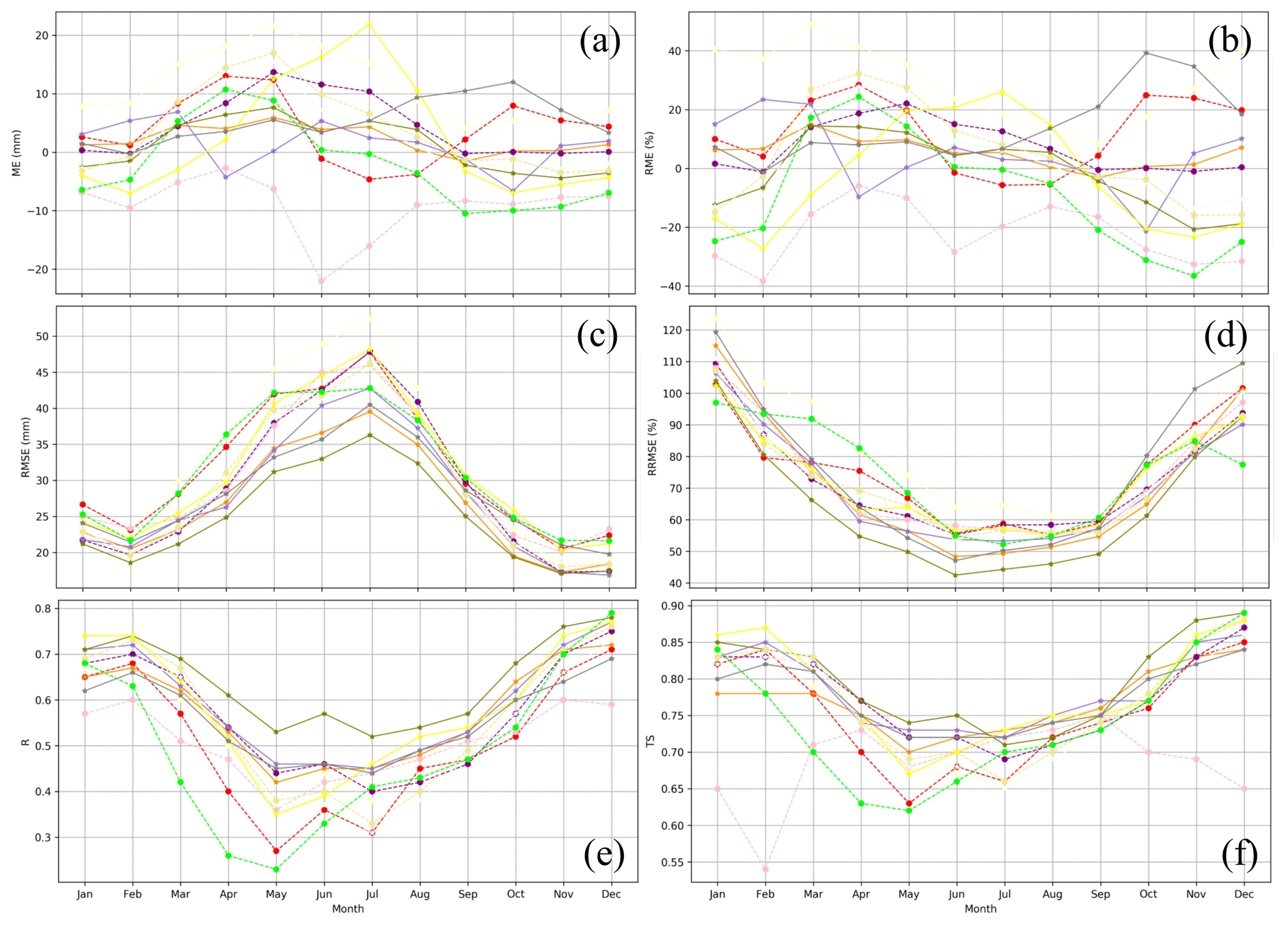
Figure 5Monthly validation metrics – ME (mm): (a); RME (%): (b); RMSE (mm): (c); RRMSE (%): (d); R: (e); TS: (f) – of ET products against flux EC ET for all sites (legend as Fig. 3k).
3.2 Synthesis method
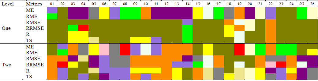
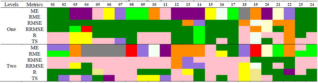
There are six validation metrics including R, TS, ME, RME, RMSE, and RRMSE. The validation values of the six metrics are categorized into levels. The level one of validation metrics has the highest R and TS values and the lowest ME, RME, RMSE, and RRMSE, while the level two of the validation metrics has the highest R and TS values and the lowest ME, RME, RMSE, and RRMSE after level one. For that, R and TS are sorted in descending order, while ME, RME, RMSE, and RRMSE are sorted in ascending order (Fig. 2a), and then the corresponding ET product of each validation metric is saved in a new table to be used to fill in Fig. 2b.
The current study proposes three steps to develop a synthesized global ET dataset. First, the ET datasets are compared based on six validated metrics to generate a matrix to indicate levels one and two of the validation metrics of all ET products over all comparison levels (Fig. 2b). For each level, there are 6 validation metrics in rows and 26 ET values of different periods and underlying conditions in columns (comparison levels), including monthly average (01), annual average (02), monthly (January–December: 03–14), land cover types (15–19), climate classes (20–23), and elevation levels (24–26). Thus, the total number of cells is 156 for each level. Each cell in the matrix represents 1 of 12 ET products that belong to this level. Then, to select ET data for further synthesis, the number and percentage of ET product occurrence at the matrix (Fig. 2b) of levels one and two were calculated (Fig. 2c). ET products were ranked in descending order based on the occurrence percentage of levels one and two (the last column in Fig. 2c). Finally, the first two or three highly ranked ET products were selected to be incorporated into the ensemble ET. For that, the selected ET products were resampled to a comparable spatial resolution if needed, and the average was used as the synthesized ET value.
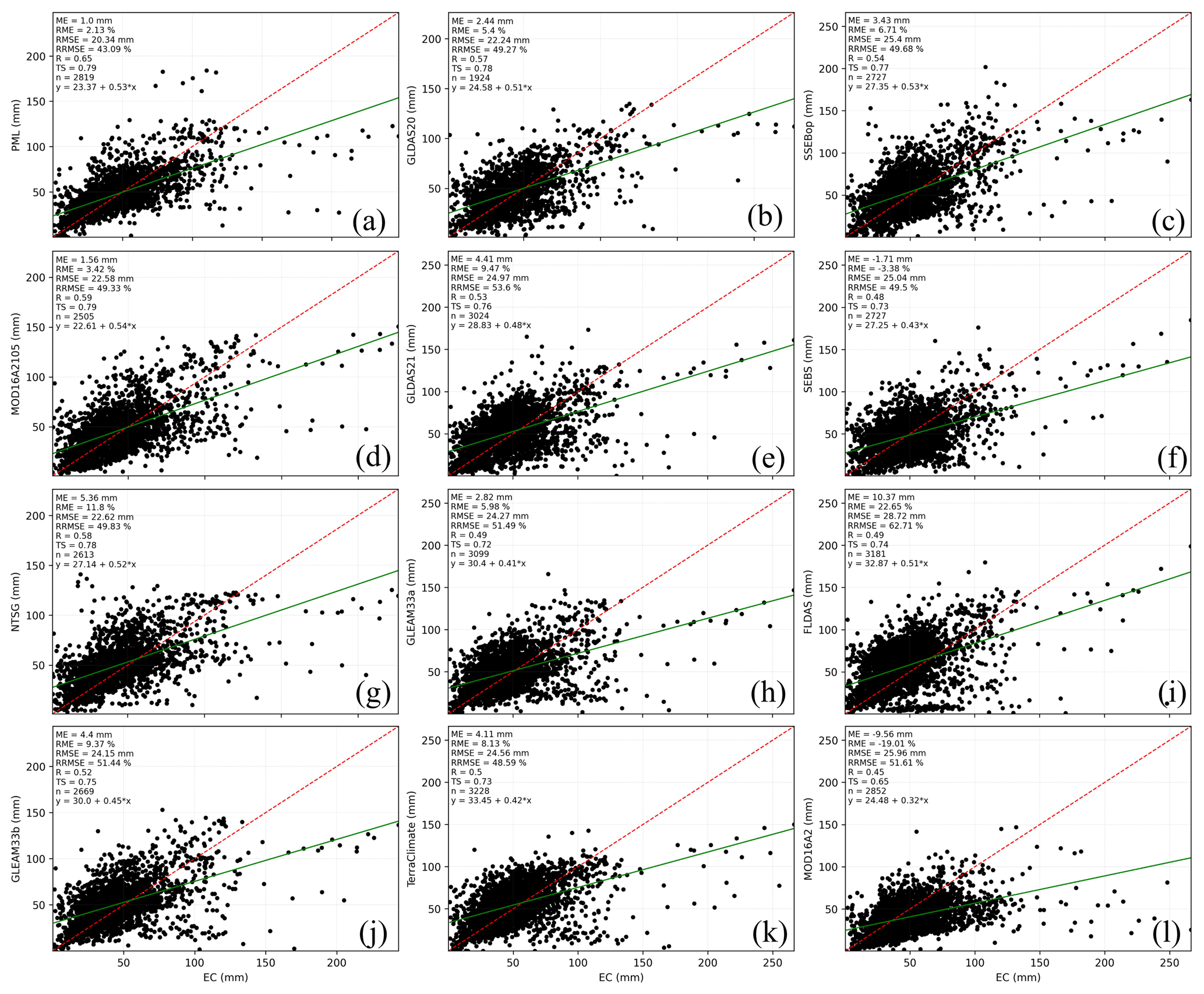
Figure 6Annually ET products against flux EC ET aggregated for all sites (subplot labels as in Fig. 4).
4.1 Assessment of existing global ET datasets
Figure 3 shows that seasonality exists and is captured well by all ET datasets with some exceptions over barren land, permanent snow and ice, and arid areas (not shown). The maximum ET occurs during July and differs according to each ET dataset. Generally, MOD16A2 represents the minimum estimated ET across all conditions, while SSEBop represents the maximum ET across all conditions except over humid regions and at elevations between 500 and 1500 m. From Figs. 4 and 6–12, the best-fitted linear regression line (solid blue line) is compared to the 1:1 line (dashed red line), and all ET datasets overestimate the flux EC ET at lower ET values and underestimate the flux EC ET at higher ET values with two exceptions. The first exception is over barren land and permanent snow and ice, where MOD16A2 underestimates and GLDAS21, GLEAM33a, and TerraClimate overestimate at both lower and higher ET values (not shown). Second, in dry subhumid areas, SSEBop (Fig. 9c3) and GLDAS21 (Fig. 9e3) overestimate at both lower and higher ET values. Applying the highest R (TS) and lowest error metric roles, MOD16A2 cannot present any role; additionally, only one contribution by the lowest RRMSE was found in February, and the highest TS was found in March for TerraClimate and GLEAM33b, respectively.
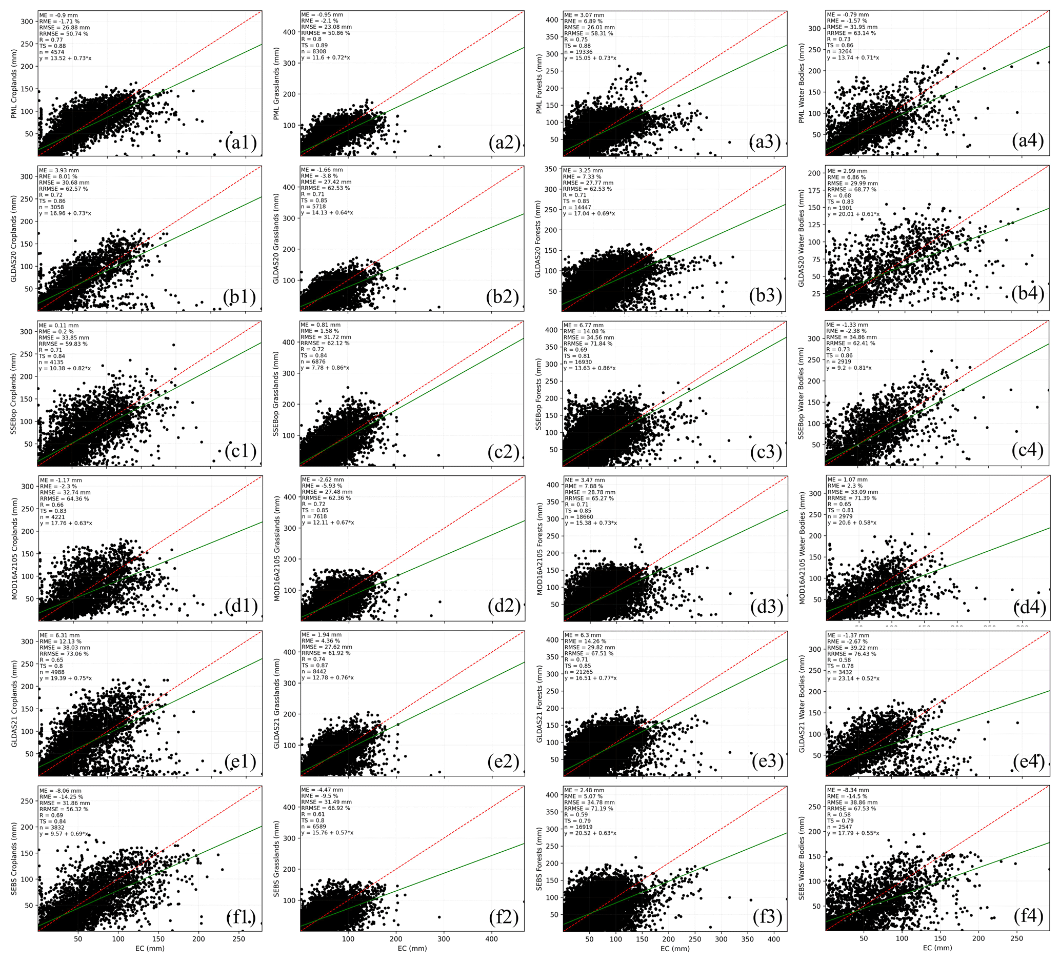
Figure 7Monthly ET products (PML: a; GLDAS20: b; SSEBop: c; MOD16A2105: d; GLDAS21: e; SEBS: f) against flux EC ET aggregated for all sites for each land cover type (croplands: 1; grasslands: 2; forests: 3; water bodies: 4).
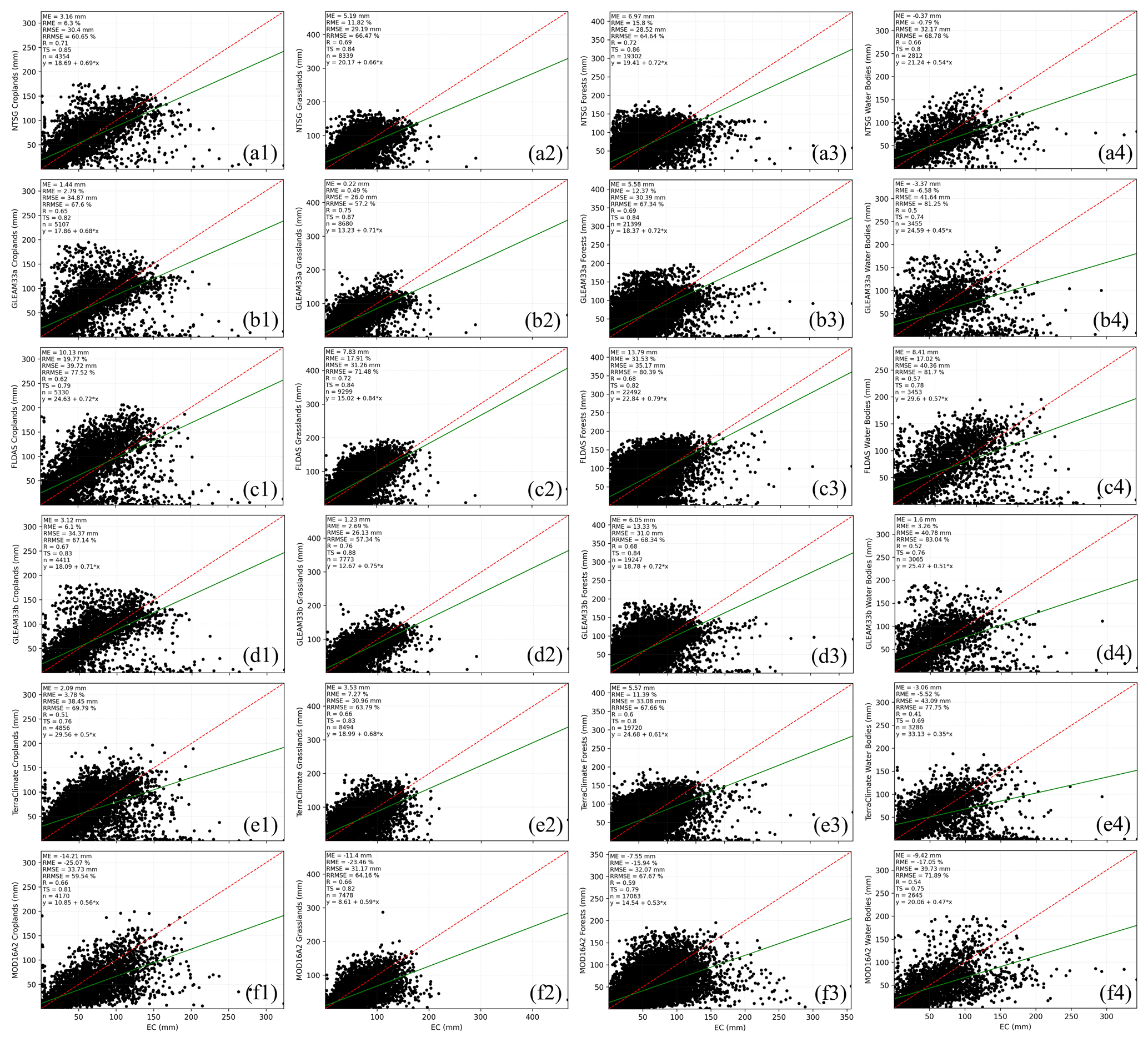
Figure 8Monthly ET products (NTSG: a; GLEAM33a: b; FLDAS: c; GLEAM33b: d; TerraClimate: e; MOD16A2: f) against flux EC ET aggregated for all sites for each land cover type (croplands: 1; grasslands: 2; forests: 3; water bodies: 4).
4.1.1 Validation by all sites' monthly ET
Figure 4 shows that only SEBS and MOD16A2 underestimate flux EC ET. PML is the dataset that best agrees with the observed ET, and it had the lowest RMSE (RRMSE). MOD16A2105 returned the smallest absolute ME, while SEBS yielded the smallest RME. Figure 5 shows there are interannual differences between certain ET product performances. MOD16A2 shows negative MEs and RMEs for all months with larger biases during March, April, and May, while FLDAS shows positive MEs and RMEs for all months with larger biases during March, April May, June, and July. For other products, the ME and RME signs vary among months; for instance, the ME and RME values of GLDAS21 are negative (underestimated) during February, September, and November and positive (overestimated) in the remaining months with larger biases during March, April, May, June, and July. The RMSE declines from January to February and then increases until July and declines again until November. The minimum RMSE values occur during February, November, and December, while the maximum values occur during June, July, and August.
For instance, the RMSE in July ranges from 36.28 to 52.41 mm for FLDAS and PML, respectively, while it ranges from 17.08 to 21.68 mm for PML and SEBS, respectively. RRMSE declines from January and reaches its minimum in June and then increases again until December except for SEBS in December. The highest values of RRMSE (>80 %) occur in January, February, November, and December except for SEBS in December, while the lowest values (<60 %) exist in June, July, and August. The R value declines from January and reaches its minimum in May; it then increases starting in August. Except for MOD16A2, all products have an R value greater than 0.60 during January, February, November, and December. SEBS has the lowest R value during March, April, May, and June, while PML yields the highest R value during all months except January and December. Except for MOD16A2 in February, which has a TS value above 0.60, as with the R value, the TS declines from January, reaches its minimum in May, and then increases again starting in August. Figures 4 and 5 show these products yield intra-annual ET variations but vary in their performance according to the selected validation metrics, which also vary among all months (from January to December).
4.1.2 Validation by all sites' annual ET
Figure 6 shows all ET products overestimate the observed ET with two exceptions: SEBS and MOD16A2. In all environmental conditions, PML has the highest R (TS) and the lowest ME (RME) and RMSE (RRMSE). Figures 4 and 6 indicate the obvious error metrics of annual-scale performances that are consistent with those that come from the monthly time step. The lowest and highest absolute values of ME (RME) for monthly ET exist in MOD16A2105 (SEBS) and FLDAS, respectively, while those for annual ET exist in PML and FLDAS, respectively. Furthermore, PML yields the largest R and TS values for monthly and annual ET, but the minimum values of R and TS were registered with TerraClimate and MOD16A2 for monthly and annual ET, respectively. This result may be attributed to the aggregation of monthly ET into annual values.
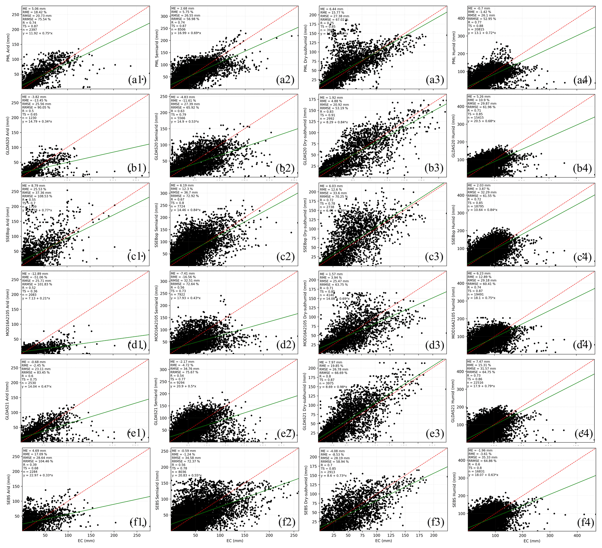
Figure 9Monthly ET products (PML: a; GLDAS20: b; SSEBop: c; MOD16A2105: d; GLDAS21: e; SEBS: f) against flux EC ET aggregated for all sites for each climate class (arid: 1; semiarid: 2; dry subhumid: 3; humid: 4).
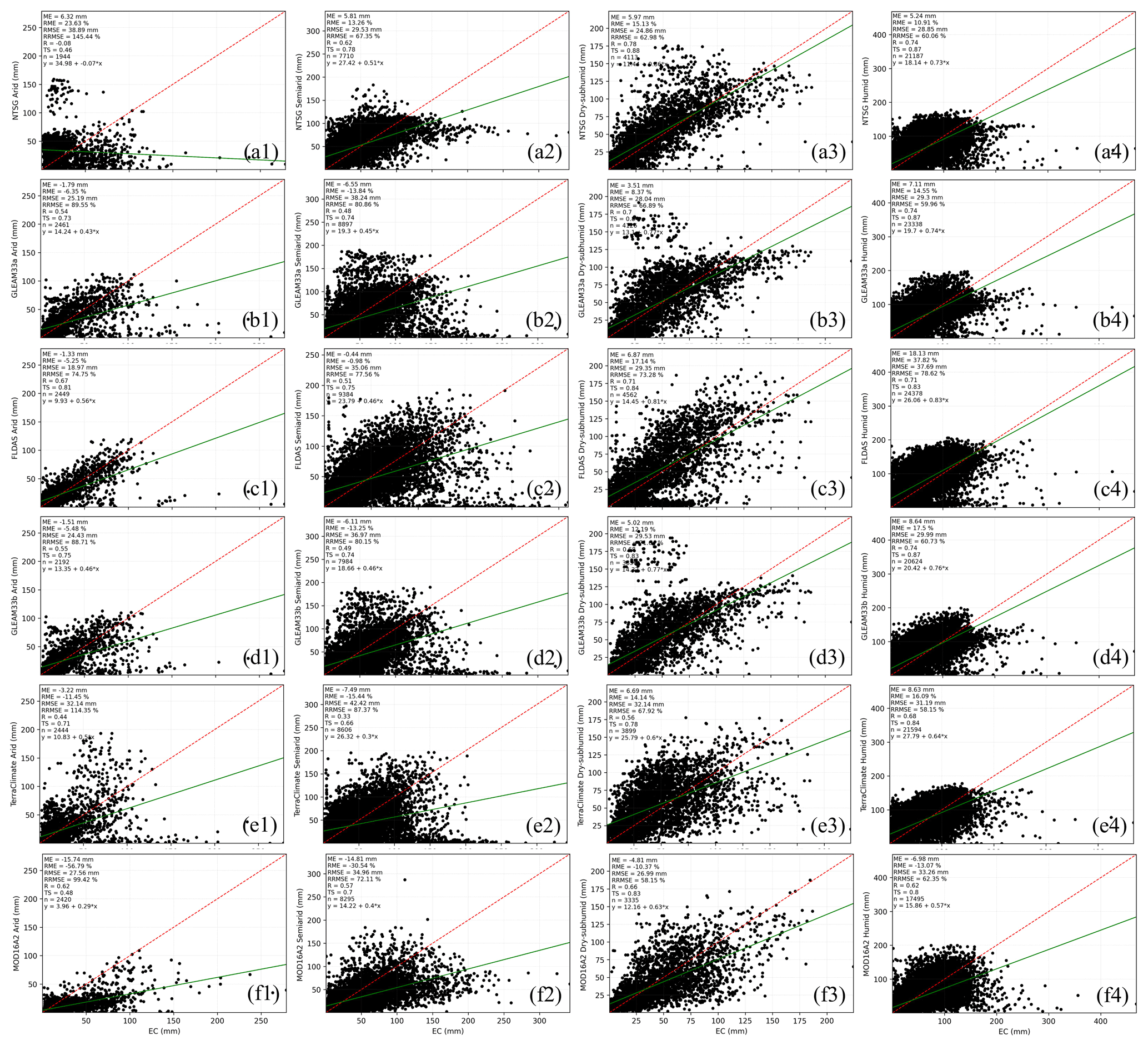
Figure 10Monthly ET products (NTSG: a; GLEAM33a: b; FLDAS: c; GLEAM33b: d; TerraClimate: e; MOD16A2: f) against flux EC ET aggregated for all sites for each climate class (arid: 1; semiarid: 2; dry subhumid: 3; humid: 4).
4.1.3 Validation by land cover types
Figures 7 and 8 show that, according to the ME (RME) sign, except for some ET products over croplands (i.e., MOD16A2, SEBS, MOD16A2105, and PML), grasslands (i.e., MOD16A2, SEBS, MOD16A2105, GLDAS20, and PML), forests (MOD16A2), and barren land and permanent snow and ice (i.e., MOD16A2105, MOD16A2, FLDAS, and GLDAS20), which underestimate the flux EC ET, the other ET products overestimate. For water bodies, MOD16A2105, GLEAM33b, GLDAS20, and FLDAS overestimate, while the other products produce underestimates. Over croplands, grasslands, and forests, PML is the best product for R (TS) and RMSE (RRMSE). Additionally, it has the highest TS over water bodies. SSEBop, GLEAM33a, SEBS, NTSG, and GLDAS20 obtained the desired ME (RME) over croplands, grasslands, forests, water bodies, and barren land and permanent snow and ice, respectively. GLEAM33a also represents the highest R (TS) with the lowest RRMSE, while GLDAS20 has the smallest RMSE over barren land and permanent snow and ice. In addition, GLDAS20 has the lowest RMSE, while SSEBop has the highest R and lowest RRMSE over water bodies; see Table 5 (level one: 15–19).
4.1.4 Validation by climate classes
Figures 9 and 10 show that SEBS, PML, NTSG, and SSEBop in arid areas and PML, NTSG, and SSEBop in semiarid areas overestimate values, while MOD16A2 and SEBS in dry subhumid areas and MOD16A2, SEBS, and PML in humid areas underestimate values; for each aridity index class, other products were the opposite. Over humid areas, PML represents the highest agreement and accurate dataset compared to the flux EC ET. Furthermore, it had the highest R (TS) in the arid and semiarid areas and the smallest RMSE (RRMSE) in semiarid areas. GLDAS20 yielded the largest R (TS) with the smallest RMSE (RRMSE) in dry subhumid regions; over these regions, MOD16A2105 presented the best ME (RME). FLDAS makes two contributions with the smallest ME (RME) and RMSE (RRMSE) in semiarid and arid areas, respectively, while GLDAS21 has only one point over arid areas where the best ME (RME) is found; see Table 5 (level one: 20–23).
4.1.5 Validation by elevation levels
Figures 11 and 12 show that MOD16A2 and SEBS over elevation levels <500 m and MOD16A2 and MOD16A2105 over elevation levels from 500 to 1500 m underestimate the values, while the other ET products overestimate the values; additionally, at elevations >1500 m, only SSEBop and NTSG overestimate the values. The ET product agreed best with the desired RMSE (RRMSE) in the PML product. Moreover, it yielded the best ME (RME) at elevations <500 m. The preferred ME (RME) over elevations of 500 m to 1500 m and elevations >500 m was obtained using SEBS and FLDAS, respectively; see Table 5 (level one: 24–26).
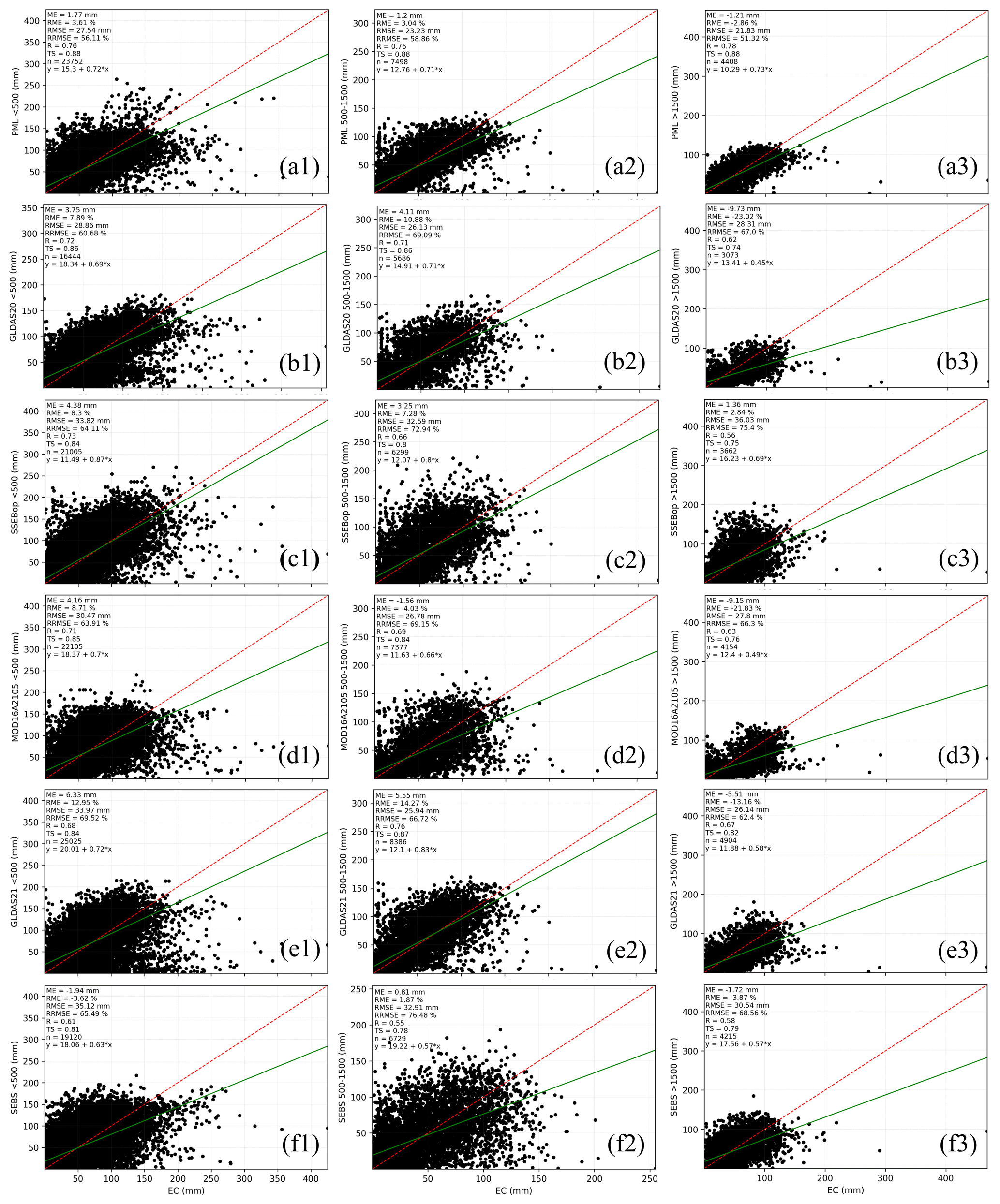
Figure 11Monthly ET products (PML: a; GLDAS20: b; SSEBop: c; MOD16A2105: d; GLDAS21: e; SEBS: f) against flux EC ET aggregated for all sites for each elevation level (<500 m: 1; 500–1500 m: 2; >1500 m: 3).
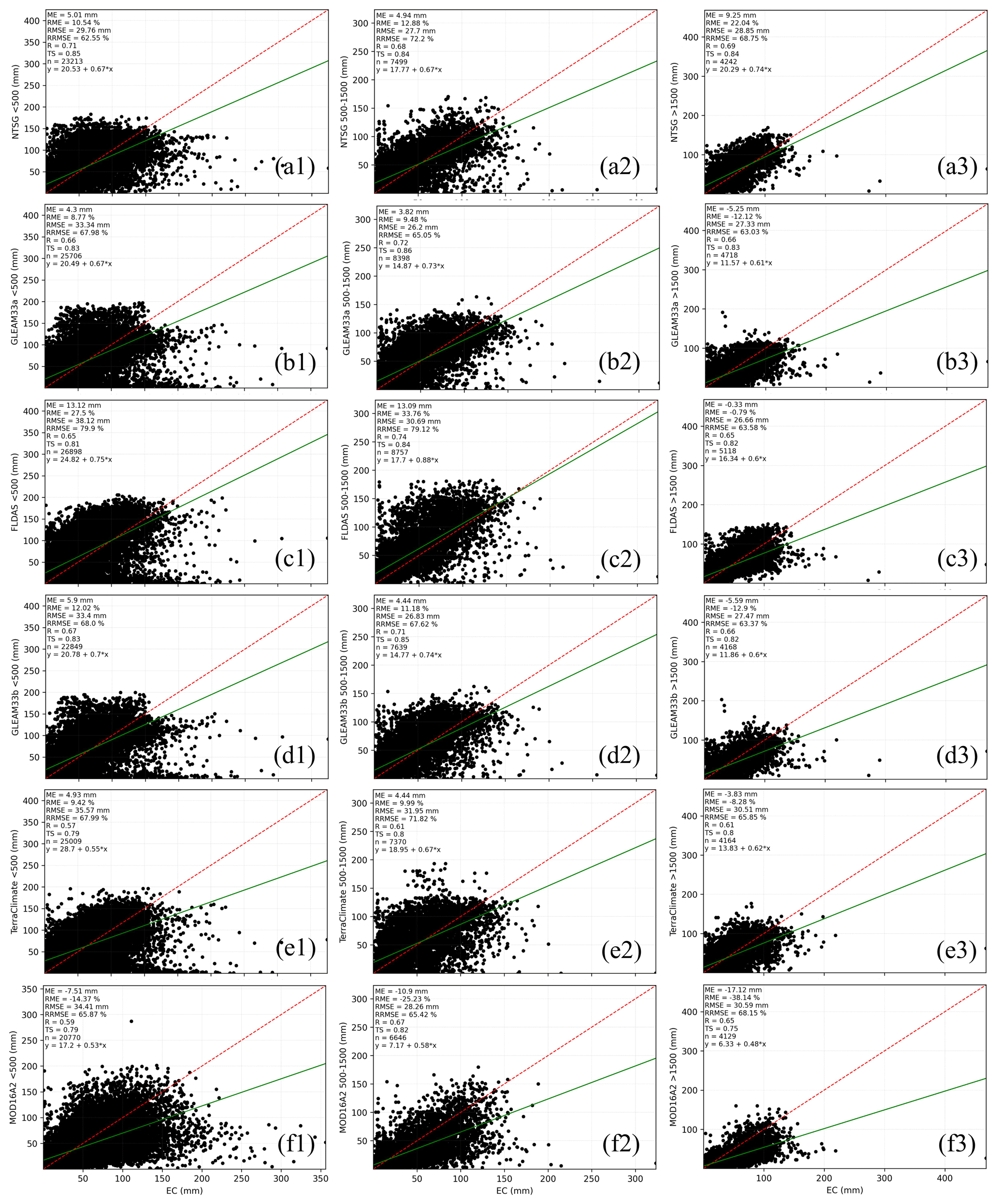
Figure 12Monthly ET products (NTSG: a; GLEAM33a: b; FLDAS: c; GLEAM33b: d; TerraClimate: e; MOD16A2: f) against flux EC ET aggregated for all sites for each elevation level (<500 m: 1; 500–1500 m: 2; >1500 m: 3).

Figure 13Monthly average flux EC ET, MOD16A2105, SSEBop, NTSG, PML, and the synthesized ET (subplot labels as in Fig. 3).
Table 5Level one and two validation metrics of the 12 ET products for monthly (01), annual (02), interannual (January–December: 03–14), land cover types (croplands, grasslands, forests, water bodies, others: 15–19), climatic classes (arid, semiarid, dry subhumid, humid: 20–23), and elevation levels (<500, 500–1500 m, >1500 m: 24–26) (cell colors as in Table 6).
4.2 Ensemble ET product
4.2.1 Ensemble steps
Table 5 provides levels one and two validation metrics of all ET products for monthly (01), annual (02), interannual (January–December: 03–14), land cover types (croplands, grasslands, forests, water bodies, others: 15–19), climatic classes (arid, semiarid, dry subhumid, humid: 20–23), and elevation levels (<500, 500–1500, >1500 m: 24–26). Each cell represents one of the validation levels (01–26) and the best-performing ET product based on the selected validation metric; see Sect. 3.
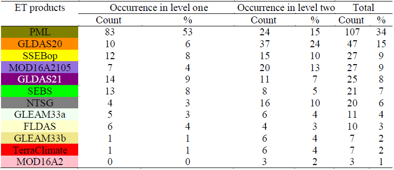
Table 7The occurrence of PML and SSEBop products and their ensemble mean from 2003 to 2017.
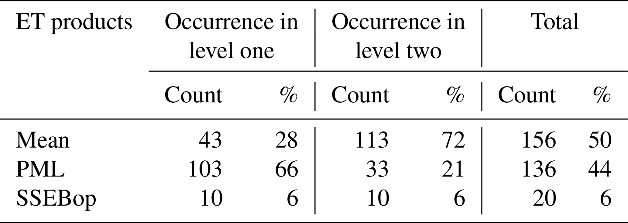
Table 8The occurrence of all ET products except PML and SSEBop products.
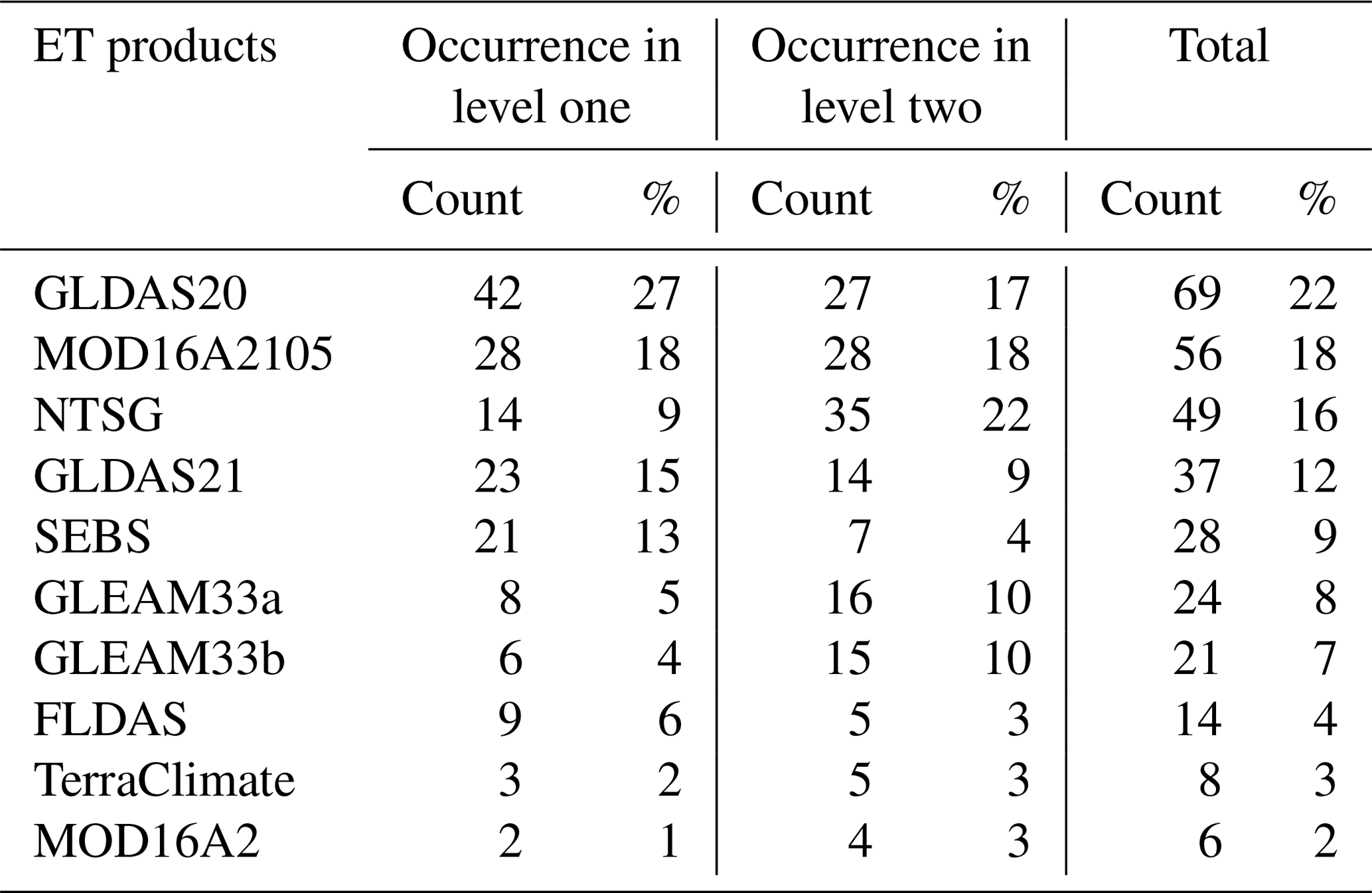
Table 9The occurrence of NTSG and MOD16A2105 products and their ensemble mean during 2001 and 2002.

Table 10The average decadal synthesized ET of monthly (mm month−1), land cover types, aridity index classes, and elevation levels (mm yr−1).

Note: monthly and annual estimates have been based on synthesized ET raster layers averaged over a decade. Land cover type, aridity index class, and elevation level estimates have been based on annual synthesized ET values extracted over all flux sites.
Table 6 shows that, according to the occurrence of ET products in level one, PML, GLDAS20, and SEBS represent the first three best-performing ET products, while, according to the occurrence of ET products in level two, GLDAS20, PML, and MOD16A2105 and, according to the total occurrence in levels one and two, PML, GLDAS20, and SSEBop are the best. For example, PML yielded the best validation metrics (the lowest ME, RME, RMSE, and RRMSE), as well as the highest R (TS) over 83 (53 %) and 24 (15 %) cells in levels one and two, respectively; thus, the total count was 107 (34 %) cells. Accordingly, the three best-performing ET products over most of all conditions are PML followed by GLDAS20 – level one: 10 (6 %); level two: 37 (24 %); total: 37 (15 %) – and SSEBop – level one: 12 (8 %); level two: 15 (10 %); total: 27 (9 %).
Since the three best-performing ET products differ in their spatial resolution and algorithms, we introduced an ensemble mean product at a 1000 m×1000 m spatial resolution that spans from 2003 to 2017 (15 years) and relies on remotely sensed models (PML and SSEBop). It should be noted that although SEBS has one point more than SSEBop in level one, it has seven fewer points than SSEBop in level two (5 %). In addition, SSEBop has a higher spatial resolution than that of SEBS. In the same manner, SSEBop and MOD16A2105 have the same performance in terms of total count, 27 (9 %), but SSEBop is higher by five points in level one.
Obviously, from Table 7, the ensemble of ET products cannot perform highly across all regions, and it had a total count of 50 %, followed by PML (44 %). Looking to the ensemble mean from Table 7 compared to PML from Table 6, the total count increased from 34 % to 50 % (+16 %), indicating that the ensemble mean, which was created from PML and SSEBop, enhanced PML performance across all conditions by 16 %, and PML itself still has the best performance by 44 %.
To introduce an ensemble product before 2003, firstly, PML and SSEBop were ignored, and the same steps were repeated. Table 8 shows that the best-performing products are GLDAS20, MOD16A2105, and NTSG in terms of the total count. Since the last two products are based on remote sensing, they were selected to create the ensemble product before 2003 at a 1000 m×1000 m spatial resolution. Although GLDAS20 agreed well with over 42 % and had the lowest maximum ME among all datasets (9.73 mm), NTSG was selected to provide the ET estimates before 2000 because it had a higher spatial resolution, so it could capture more spatial details than GLDAS20.
Table 9 shows that the ensemble ET for 2001 and 2002 performed better than the original ET products with values of 62 %, 38 %, and 50 % for level one, level two, and the total, respectively. For the periods before 2001, NTSG can be used from 1982 to 2001 or GLDAS20 can be used instead. Hence, remote-sensing-based long-term ensemble ET can be synthesized from PML and SSEBop between 2003 and 2017 and MOD16A2105 and NTSG between 2001 and 2002. SSEBop can be used after 2017, while before 2001, NTSG can be used.
4.2.2 Contribution of ET datasets to the synthesized ET
The synthesized ET dataset was created at a 1000 m×1000 m spatial resolution from 1982 to 2019 based on remotely sensed ET products. PML, SSEBop, MOD16A2105, and NTSG were augmented together to create the new dataset. Since SSEBop and MOD16A2105 have a 1000 m×1000 m spatial resolution, PML was upscaled and NTSG was downscaled by pixel average and nearest-neighbor resampling techniques in GEE, respectively. The synthesized ET was fully contributed by SSEBop for the years 2018 and 2019 and by NTSG from 1982 to 2000, while for the years 2001 and 2002, it was contributed by the simple mean of MOD16A2105 and NTSG. Finally, between 2003 and 2017, the value represents the simple mean of PML and SSEBop.
Since the synthesized ET performance was governed by each ET product(s) for the corresponding year from 1994 to 2019 (25 years), when the ET EC fluxes were available, most of the performance comes from PML and SSEBop for the 15 years from 2003 to 2017 (60 %), from MOD16A2105 and NTSG for 2 years (2001 and 2002; 8 %), from SSEBop for individual values in years 2018 and 2019 (8 %), and from NTSG for 7 years (24 %) from 1994 to 2000.
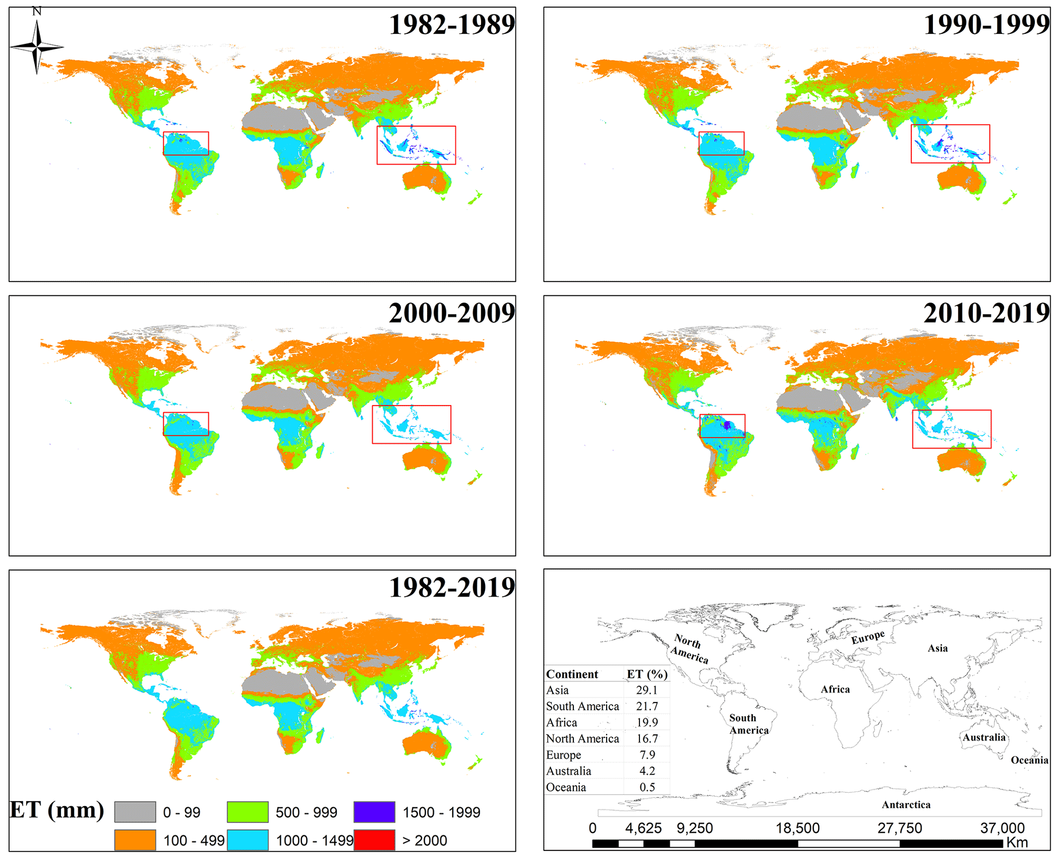
Figure 14Decadal and long-term synthesized ET. The last plot shows the continental scale used to create Table 11 accompanied by the percent of ET over each continent except Antarctica for the period 1982–2019. Use the following link of the GEE application to preview these maps: https://elnashar.users.earthengine.app/view/synthesizedet (last access: 21 January 2021).
Table 11Statistics of the decadal and long-term synthesized ET (mm).
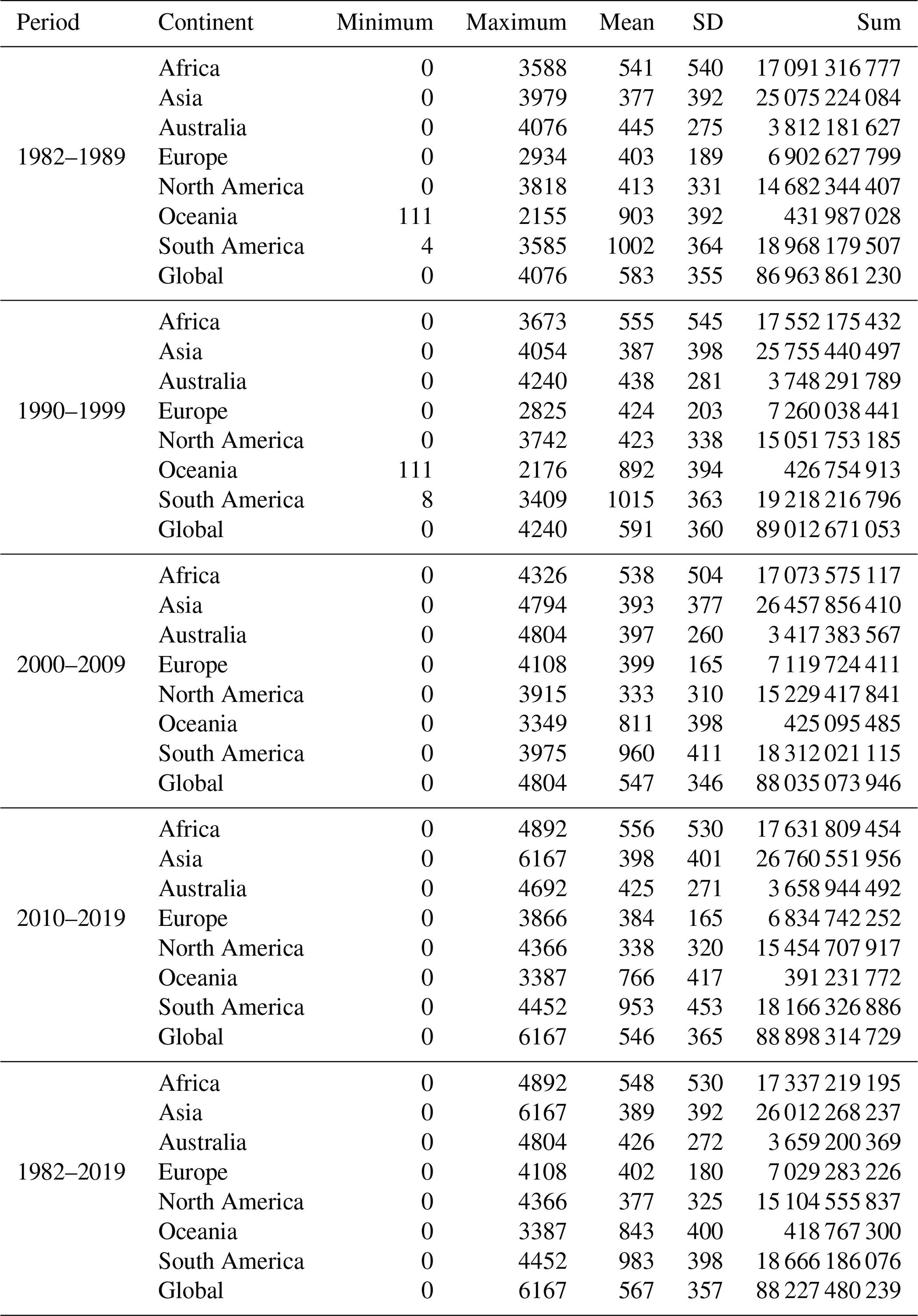
Table 12Same as Table 5 but MOD16A2 replaced by the synthesized ET (cell colors as in Table 13).
Note: MOD16A2 ignored according to Sect. 4.1.
Table 13Same as Table 6 but MOD16A2 replaced by the synthesized ET and based on Table 12.

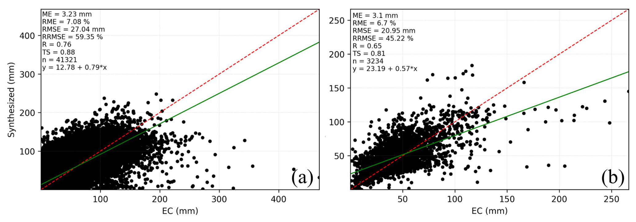
Figure 15Monthly (a) and annually (b) synthesized ET against flux EC ET aggregated for all sites.
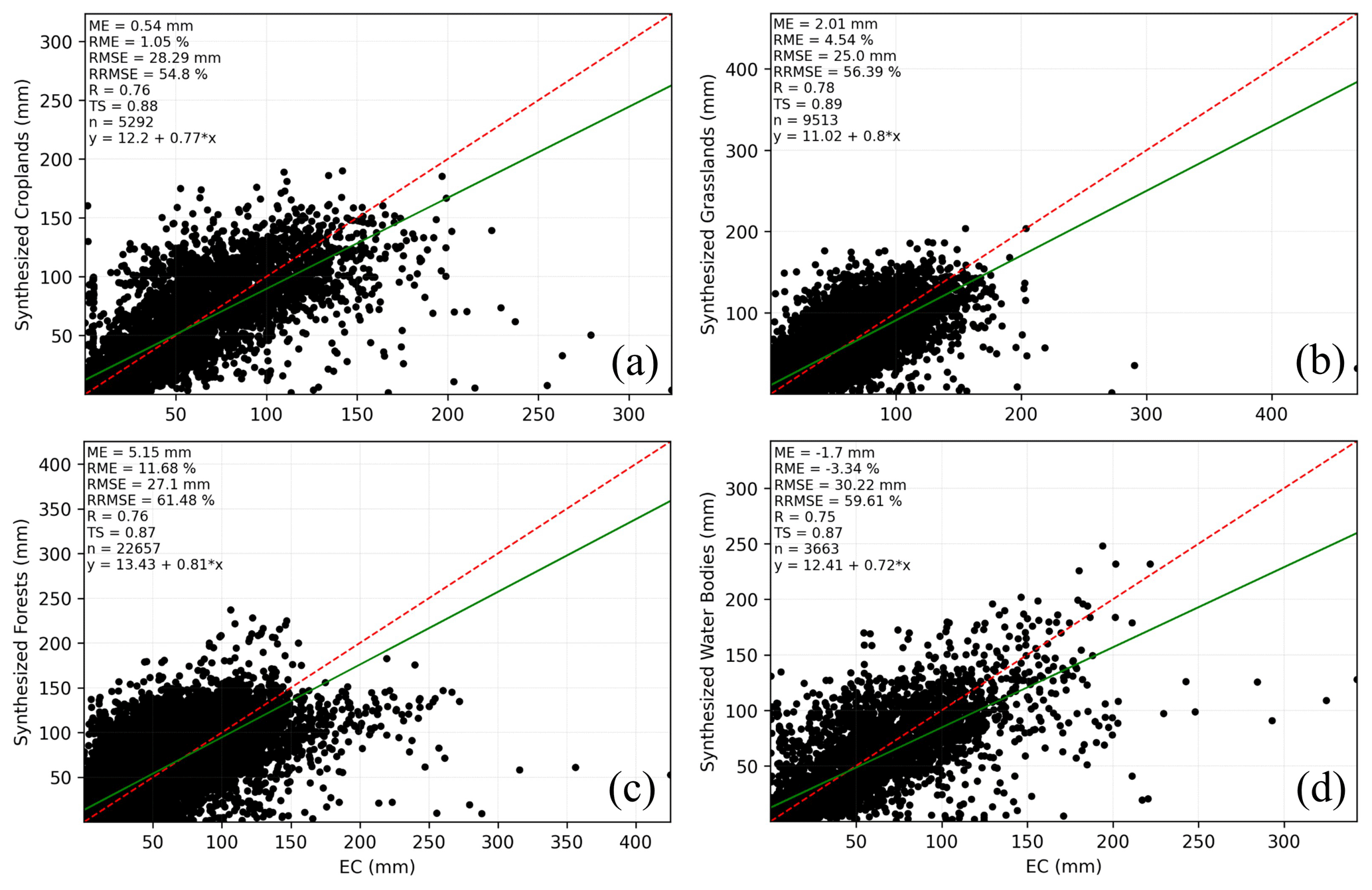
Figure 16Monthly synthesized ET against flux EC ET aggregated for all sites for each land cover type (croplands: a; grasslands: b; forest: c; water bodies: d).
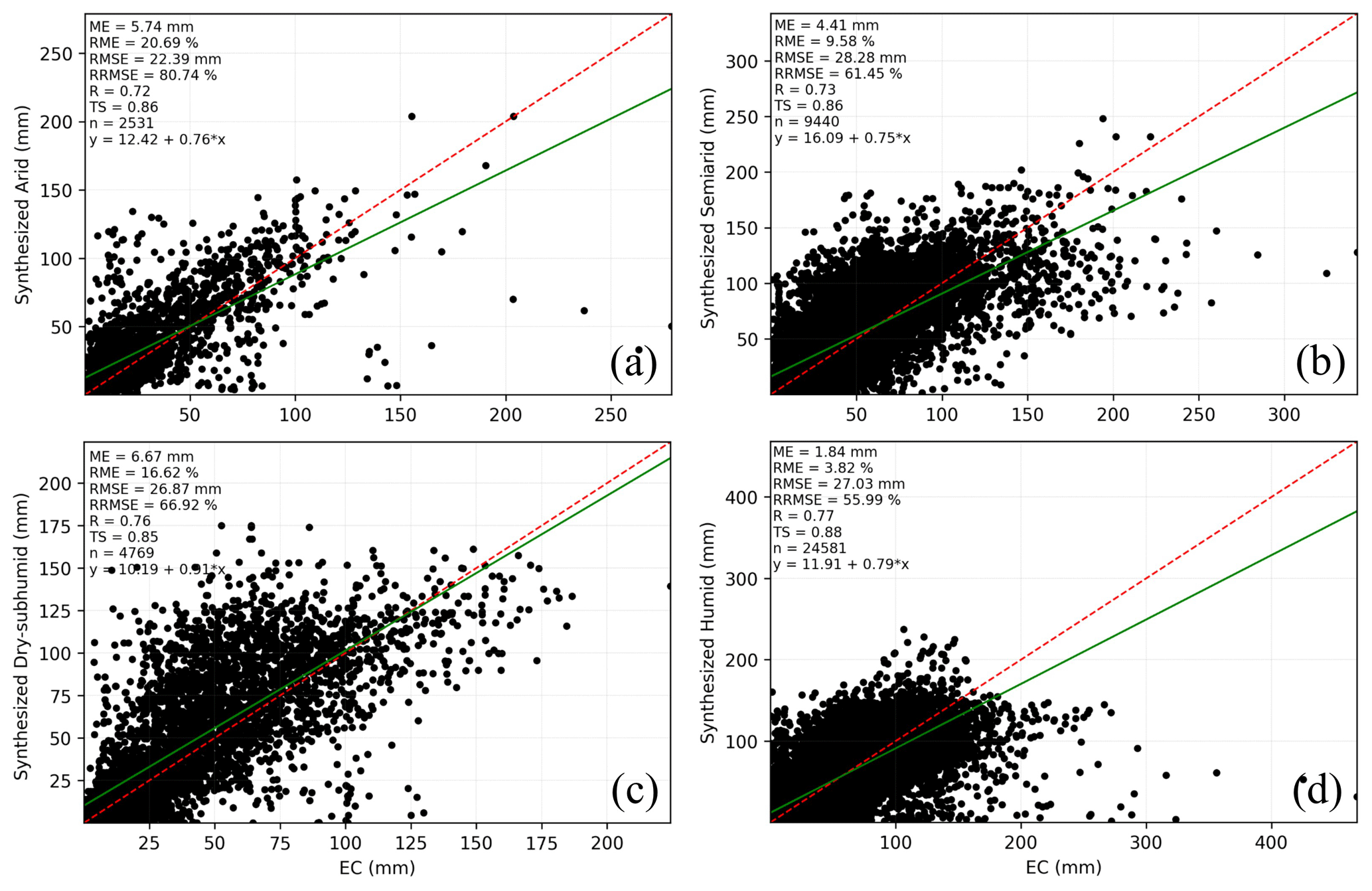
Figure 17Monthly synthesized ET against flux EC ET aggregated for all sites for each climate class (arid: a; semiarid: b; dry subhumid: c; humid: d).
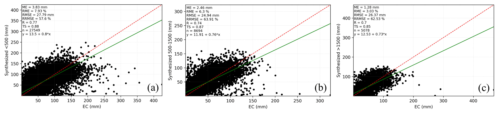
Figure 18Monthly synthesized ET against flux EC ET aggregated for all sites for each elevation level (<500 m: a; 500–1500 m: b; >1500 m: d).
4.2.3 Synthesized global ET product
Figure 13 shows, looking to July and except over barren land, permanent snow and ice, and arid areas (not shown), that the maximum value of the synthesized ET lies between SSEBop, which yields the largest ET during all months, and PML. Hence, the long-term monthly synthesized ET performance is affected by PML and SSEBop more than by NTSG and MOD16A2105, as mentioned in Sect. 4.2.2.
Table 10 provides the average monthly and annual synthesized ET (mm month−1), land cover types, aridity index classes, and elevation levels (mm yr−1). The average annual ET from 1982 to 2019 is 567 mm yr−1. July represents the maximum synthesized ET (Fig. 13). Table 10 also provides average annual ET for land cover types calculated from flux sites. Across land cover types, croplands are higher than forests, followed by grasslands, where the average synthesized ET was 597, 548, and 542 for croplands, forests, and grasslands, respectively. Low synthesized ET values across arid areas (average = 392 mm yr−1) can be attributed to low vegetation cover. It should be noted that Table 10 does not represent the perfect calculation of ET over each land cover class because the total number of fluxes for each class was not distributed well; for instance, in the arid areas, there were 35 (5 %) fluxes, while in the humid area, there were 361 (56 %) fluxes.
Figure 14 shows the decadal (1982–1989, 1990–1999, 2000–2009, and 2010–2019) and long-term (1982–2019) average synthesized ET maps worldwide except for Antarctica. Regarding the spatial distribution, the higher ET is shown in Malaysia, Singapore, and Indonesia and the northern part of South America. During the first and second decades, the synthesized ET is based on the NTSG product; thus, the same spatial distribution was observed. Although PML and SSEBop mainly contribute the synthesized ET between 2003 and 2017, there is little difference in their spatial distributions, in which higher ET can be observed during 2010–2019 over the northern parts of South America.
Table 11 shows statistics of the maps provided in Fig. 14 for all continents except Antarctica. The standard deviation is higher over Africa, followed by Oceania and Asia. The mean values of the synthesized ET are sequenced from South America, followed by Oceania and Africa. The maximum value of the synthesized ET is recorded over Asia, followed by Africa and Australia. The total ET values are 29.1 %, 21.7 %, 19.9 %, 16.7 %, 7.9 %, 4.2 %, and 0.5 % for Asia, South America, Africa, North America, Europe, Australia, and Oceania, respectively.
4.2.4 Validation of the synthesized ET
Figures 15–18 show that the synthesized ET agreed well with the observed data, in which the R (TS) ranged between 0.70 (0.85) and 0.78 (0.89) except at the annual time step (Fig. 15b) and over barren land and permanent snow and ice (not shown), where R (TS) was 0.65 (0.81) and 0.68 (0.80), respectively. Based on the ME sign, the value was underestimated only over water bodies. The magnitude of ME (RME) ranged between 0.54 mm (1.05 %) and 6.76 mm (16.62 %), while the RMSE (RRMSE) ranged from 20.95 mm (45.22 %) to 30.12 mm (59.61 %). Looking at the regression line equation, with no exceptions, the synthesized ET overestimated the flux EC ET at lower ET values and underestimated the flux EC ET at higher ET values. As mentioned above, even the long-term synthesized ET cannot perform best across all comparison levels (Tables 12 and 13).
During the periods 2018–2019 and before 2001, the synthesized ET performance came from the original datasets of SSEBop and NTSG, respectively. The ensemble mean has a total count of 50 % over the periods 2003–2017 and 2001–2002 compared to the original datasets, indicating that it can perform better than other ET products over half of all comparison levels (see Tables 7 and 9).
Figure 19 presents a monthly comparison between the synthesized ET with the country-based ET products over China and the United States, as well as over the African continent. In general, the synthesized ET returned higher agreement (R and TS) and accuracy (RMSE) with the flux EC ET than did the other ET products (CR, SSEBop, and FAO WaPOR). Moreover, it has lower biases over the United States and the African continent.

Figure 19Monthly comparison between the synthesized ET (a, c, e) and CR (b), SSEBop (d), and FAO WaPOR (f) ET products against flux EC ET aggregated for all sites over China (a, b), the USA (c, d), and the African continent (e, f).
Since global land ET plays a paramount role in the hydrological cycle, its accurate estimation is essential for further studies. Although there are many global ET products that have been derived from remote sensing models, land surface models, and hydrological models, they differ in their algorithms, parameterization, and temporal span, and none of these products can be used for a long time with a reasonable spatial resolution and lower uncertainty. In this study, we ensemble the best-performing currently available global ET products at a reasonable spatial resolution (kilometer) as one consistent global ET dataset covering a long temporal period. Users can use this dataset assuredly without looking at other datasets and performing additional assessments.
We used a high-quality dataset of global flux towers as a site-pixel-level validation for certain global ET products (Leuning et al., 2008; Zhang et al., 2010; Ershadi et al., 2014; Michel et al., 2016) to assess them and select the best products to create a synthesized ET covering a long temporal period. For that, a matrix of 6 validation criteria and 26 comparison levels was created, and then levels one and two of the validation metrics were used to select the best-performing products. Finally, by the simple mean of the products that performed best over the different periods, the synthesized ET was created.
Among all global ET products investigated in this study, the products that performed best are PML, GLDAS20, SSEBop, MOD16A2105, GLDAS21, SEBS, and NTSG (Table 6). From the perspective of all comparison levels, the performance of these products varied, and no single product performed well across all land surface types and conditions (Vinukollu et al., 2011a; Li et al., 2018). The PML represents the ET product with the highest agreement with lower ME (RME) and RMSE (RRMSE) values, followed by the synthesized ET (Tables 12 and 13); however, it should be noted that PML estimates span a 15-year period, while the synthesized ET presents longer estimates from 1982 to 2019 (38 years).
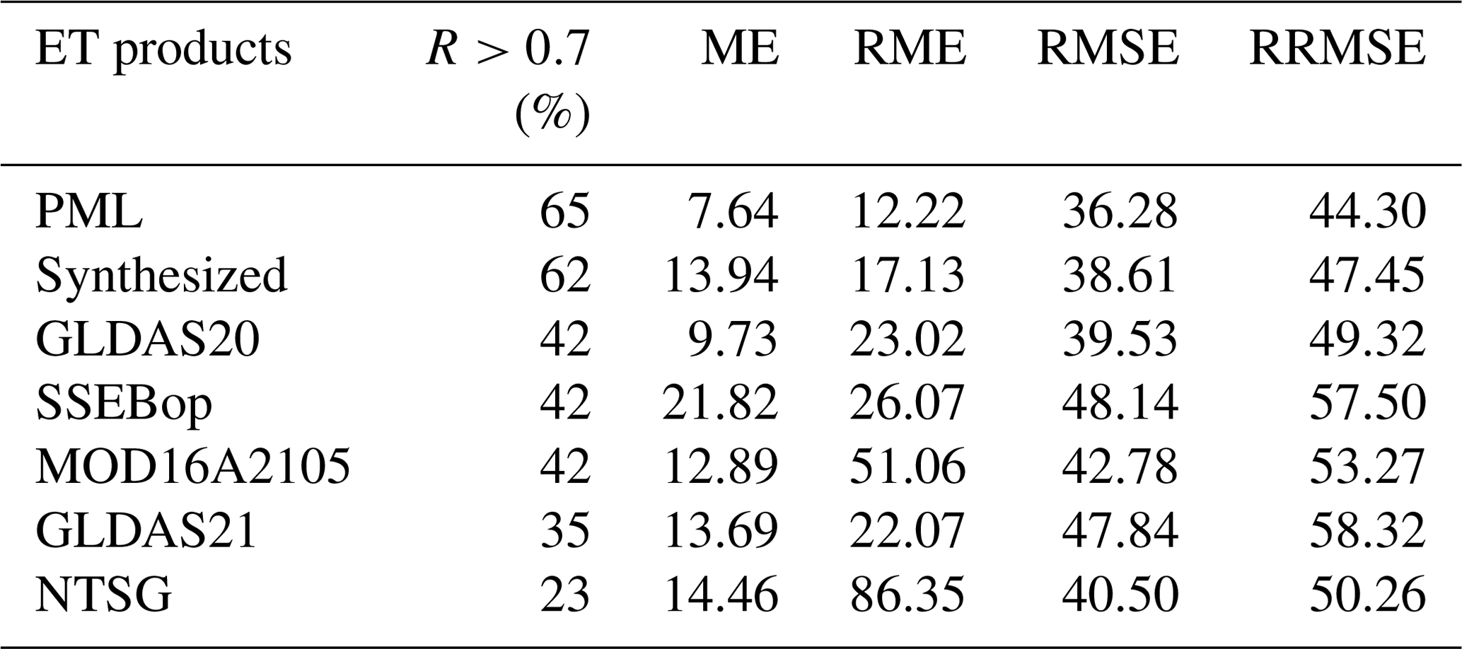
The main advantage of the new dataset is that, for the first time, a synthesized remotely sensed ET product with a reasonable spatial resolution and lower long-term uncertainties has been provided, in which the maximum absolute ME (RME) and RMSE (RRMSE) values are 13.94 mm (17.13 %) and 38.61 mm (47.45 %), respectively. Furthermore, it agreed well (R>0.70) in 62 % of all comparison levels (Table 14). This dataset can provide ensemble ET estimates for all land cover types for which MOD16A2105 does not provide ET estimates, including over water bodies and desert areas. Moreover, a comparison between the synthesized ET and CR, SSEBop, and FAO WaPOR ET products over China, the United States, and the African continent proved that the synthesized ET outperformed these products in terms of a higher agreement, higher accuracies, and lower biases. Hence, the synthesized ET can play an essential role, especially for regional- and global-scale studies, over a long time period (1892–2019).
Table 14Percentage of R more than 0.70 and the maximum absolute value of ME (mm), RME (%), RMSE (mm), and RRMSE (%) across all comparison levels (01–26) of the highly performing ET products and the synthesized ET.
The synthesized ET used SSEBop ET for the years 2018 and 2019 and NTSG from 1982 to 2000 because NTSG is the only remotely sensed global ET product available and has a good spatial resolution compared to GLDAS20. It is the simple mean of MOD16A2105 and NTSG for the years 2001 and 2002 and the simple mean of PML and SSEBop between 2003 and 2017 (see Tables 7 and 9).
Because the ET was synthesized during the first and second decades, as well as the year 2000, and is based on NTSG resampled to a 1 km spatial resolution to be comparable with other products, future improvements may be focused on statistical downscaling of NTSG during this period. Moreover, since different datasets were selected due to data availability, also future improvements may be focused on the adjustment of the ensemble means particularly for long-term pixel-based studies.
All data used in this study are freely available; see Sect. 2 and Appendix A. The synthesized ET is available at https://doi.org/10.7910/DVN/ZGOUED (Elnashar et al., 2020) and as a GEE application from the following link: https://elnashar.users.earthengine.app/view/synthesizedet (last access: 21 January 2021). In addition, it can be accessed in the GEE JavaScript editor (the updated link is embedded in the GEE application interface). Through this application, the user can query and display, as well as download, the synthesized ET. It should be noted that SSEBop and NTSG datasets are not available in Earth Engine, so they were uploaded as assets in GEE for this purpose.
In the current study, a site-pixel-level validation was conducted for certain global ET products across a variety of land surface types and conditions to select the best performing ET products and then produce a global long-term synthesized ET dataset. To apply a comprehensive evaluation from different perspectives, land cover types, climate, and elevations were classified into five, four, and three classes, respectively. According to six comprehensive validation criteria, the evaluated ET products were ranked based on the lowest error metrics and highest accuracy and consistency over different classification levels to choose the ensemble members over different times.
The average annual ET from 1982 to 2019 is 567 mm yr−1. Although no product performed better in terms of all selected validation criteria in all classification levels, PML, GLDAS20, SSEBop, MOD16A2105, GLDAS21, SEBS, and NTSG are the sequence of their performances. The synthesized ET from PML, SSEBop, MOD16A2105, and NTSG agreed with the flux EC ET with R values higher than 0.70, a maximum ME (RME) of 13.94 mm (17.13 %), and a maximum RMSE (RRMSE) of 38.61 mm (47.45 %) over 62 % of all comparison levels as a remote-sensing-based ET product spanning from 1982 to 2019 with the highest agreements and accuracies and lower biases over most of the land surface types and conditions. It performs well when compared with country-based and continental ET products over China, the United States, and the African continent. However, the further synthesis of local ET products is encouraged if regional ET products are available.
The results from this study provide a better understanding of the high-performing ET products in each land cover type, elevation level, and climate region, as well as monthly, annual, and interannual time steps. Hence, this study provides an ET product that can be used to improve the quality of ET at regional and global levels and, consequently, can be used to improve agriculture, water resource management, and climate change studies.
A summary of ET datasets used in this research is presented here. It should be noted that except for SSEBop, SEBS, NTSG ET, and GLEAM, which are downloaded from their providers, other datasets are available from the Earth Engine Data Catalog through the following link: https://developers.google.com/earth-engine/datasets/catalog (last access: 21 January 2021). Each dataset in GEE has Earth Engine Snippet as following:
-
MOD16A2 ET V6:
ee.ImageCollection(“MODIS/006/MOD16A2”)
-
MOD16A2 ET V105:
ee.ImageCollection(“MODIS/NTSG/MOD16A2/105”)
-
PML ET:
ee.ImageCollection(“CAS/IGSNRR/PML/V2”)
-
GLDAS ET V20:
ee.ImageCollection(“NASA/GLDAS/V20/NOAH/ G025/T3H”)
-
GLDAS ET V021:
ee.ImageCollection(“NASA/GLDAS/V021/NOAH/ G025/T3H”)
-
FLDAS ET:
ee.ImageCollection(“NASA/FLDAS/NOAH01/C/GL/ M/V001”)
-
TerraClimate ET:
ee.ImageCollection(“IDAHO_EPSCOR/TERRACLI MATE”)
A1 MOD16 ET
The Moderate Resolution Imaging Spectroradiometer (MODIS) Global Evapotranspiration Project (MOD16A2) estimates terrestrial ET as the sum of evaporation and plant transpiration. MOD16A2 ET uses the Penman–Monteith model, which includes MODIS remotely sensed data (e.g., vegetation, surface albedo, and land cover classification) and daily meteorological reanalysis. There are two products of MOD16A2 ET (V6 and V105) at an 8 d temporal resolution, but they differ in their spatial resolution and temporal coverage (Mu et al., 2011, 2014b). V6 spans from 2001 until now at a 500 m×500 m spatial resolution and is provided by NASA Land Processes Distributed Active Archive Center (LP DAAC) at the United States Geological Survey (USGS) Earth Resources Observation and Science (EROS) center; it can be downloaded from https://doi.org/10.5067/MODIS/MOD16A2.006. V105 estimates span the period from 2001 to 2014 at a 1000 m×1000 m spatial resolution and are provided by the Numerical Terradynamic Simulation Group (NTSG) at the University of Montana in conjunction with the NASA Earth Observing System (Mu et al., 2014a).
A2 PML ET
The Penman–Monteith–Leuning (PML) ET product partitions ET into three components: plant transpiration, soil evaporation, and intercepted rainfall by the canopy, as well as water evaporation. PML data span from 2002 to 2017 at a 500 m×500 m spatial resolution and an 8 d temporal resolution (Zhang et al., 2019).
A3 SSEBop
The operational Simplified Surface Energy Balance (SSEBop) model is based on the Simplified Surface Energy Balance (SSEB) approach with a unique parameterization for operational applications. Using a thermal index approach, it combines ET fractions generated from remotely sensed MODIS land surface temperature (LST) acquired every 10 d with reference ET from global weather datasets. The SSEBop uses predefined, seasonally dynamic, boundary conditions that are unique to each pixel for the hot and cold reference points (Senay et al., 2007, 2011, 2013, 2020). SSEBop estimates are from 2003 at a 0.0096∘ × 0.0096∘ (≈1 km) spatial resolution and a monthly temporal resolution. Data were provided by the Early Warning and Environmental Monitoring Program via the United States Geological Survey and can be downloaded from the following website https://earlywarning.usgs.gov (last access: 21 January 2021).
A4 SEBS
The Surface Energy Balance System (SEBS) is an approach designed to estimate ET from the evaporative fraction using satellite remote sensing augmented by meteorological data at corresponding scales (Su, 2002). MODIS-LST and the Normalized Difference Vegetation Index (NDVI), GLASS-LAI (leaf area index), GLAS global forest height, GlobAlbedo, and ERA-Interim meteorological data have been used in these ET calculations with the revised SEBS algorithm (X. Chen et al., 2013, 2014, 2019). SEBS is available during the period from 2000 to 2017 at a 5 km×5 km spatial resolution and monthly temporal resolution. It is copyrighted by the Institute of Tibetan Plateau Research, Chinese Academy of Sciences, and is available at http://en.tpedatabase.cn (last access: 21 January 2021).
A5 NTSG ET
The Numerical Terradynamic Simulation Group (NTSG) ET data are based on an algorithm that estimates transpiration from the canopy and evaporation from soil using a modified Penman–Monteith model and evaporation from open water using a Priestley–Taylor model. These algorithms were applied globally using the Advanced Very High-Resolution Radiometer (AVHRR) Global Inventory Modeling and Mapping Studies (GIMMS) NDVI, NCEP/NCAR (National Centers for Environmental Prediction/National Center for Atmospheric Research) Reanalysis daily surface meteorology, and NASA GEWEX (Global Energy and Water Exchanges) Surface Radiation Budget Release-3.0 solar radiation inputs (Zhang et al., 2009, 2010). NTSG estimates cover a period from 1982 to 2013 at a spatial resolution of 8 km×8 km and a monthly temporal resolution. It is produced by NTSG at the University of Montana and can be retrieved from http://files.ntsg.umt.edu/ (last access: 21 January 2021).
A6 GLEAM
The Global Land Evaporation Amsterdam Model (GLEAM) is physically based on an algorithm that estimates ET components separately (i.e., transpiration, interception loss, bare soil evaporation, snow sublimation, and open-water evaporation). The potential evaporation is estimated by the Priestley–Taylor equation based on observations of surface net radiation and near-surface air temperature and is then converted into actual evaporation based on the evaporative (soil) stress factor. The soil stress factor is based on microwave vegetation optical depth and simulated root-zone soil moisture calculated from a multilayer water balance model. Separately, interception loss is calculated based on vegetation and rainfall observations. There are two datasets available for GLEAM (i.e., v3.3a, and v3.3b) that differ only in their forcing and temporal coverage. GLEAM v3.3a spans from 1980 to 2018 and relies on reanalysis radiation and air temperature, a combination of gauge-based, reanalysis, and satellite-based precipitation, and satellite-based vegetation optical depth, while v3.3b spans from 2003 to 2018, and its forcing factors are the same as v3.3a except for radiation and air temperature which are based on remotely sensed data. Both v3.3a and v3.3b estimates are provided at a monthly temporal resolution and a 0.25∘ × 0.25∘ (≈25 km) spatial resolution (Miralles et al., 2011a, b; Martens et al., 2017).
A7 GLDAS ET
The Global Land Data Assimilation System (GLDAS) generates optimal fields of land surface states and fluxes using advanced land surface modeling and data assimilation techniques by ingesting satellite and ground-based observational data products. GLDAS version 2 has two components (GLDAS-2.0 and GLDAS-2.1) at a 0.25∘ × 0.25∘ (≈25 km) spatial resolution and a 3 h temporal resolution. GLDAS-2.0 is reprocessed with the updated Princeton Global Meteorological Forcing Dataset and upgraded Land Information System version 7. The model simulation was initialized from 1 January 1948 to 31 December 2010 using soil moisture and other state fields from the LSM climatology for that day of the year. The simulation used the common GLDAS datasets for land cover (MCD12Q1), land-water mask (MOD44W), and soil texture and elevation (GTOPO30). The GLDAS-2.1 simulation started on 1 January 2000 and lasted until 31 December 2019 using the conditions from the GLDAS-2.0 simulation. This simulation was forced with the National Oceanic and Atmospheric Administration (NOAA)/Global Data Assimilation System (GDAS) atmospheric analysis, disaggregated Global Precipitation Climatology Project (GPCP) precipitation, and Air Force Weather Agency's AGRicultural METeorological modeling system (AGRMET) radiation. The MODIS-based land surface parameters were used in the current GLDAS-2.x products, while the AVHRR base parameters were used in previous GLDAS-2 products before October 2012 (Rodell et al., 2004).
A8 FLDAS ET
The Famine Early Warning Systems Network (FEWS NET) Land Data Assimilation System (FLDAS) dataset uses remotely sensed and reanalysis inputs to drive land surface models. It includes information on many climate-related variables, including evapotranspiration, moisture content, humidity, average soil temperature, and total precipitation rate. For forcing data, this FLDAS dataset uses a combination of the new version of Modern-Era Retrospective analysis for Research and Applications version 2 (MERRA-2) data and Climate Hazards Group InfraRed Precipitation with Station (CHIRPS) data, a quasi-global rainfall dataset designed for seasonal drought monitoring and trend analysis (McNally et al., 2017). FLDAS is provided at a 0.1∘ × 0.1∘ (≈10 km) spatial resolution and monthly temporal resolution during the period 1982–2019.
A9 TerraClimate ET
TerraClimate ET is estimated based on a monthly one-dimensional soil water balance for global terrestrial surfaces, which incorporates evapotranspiration, precipitation, temperature, and interpolated plant extractable soil water capacity. The water balance model is very simple and does not account for heterogeneity in vegetation types or their physiological responses to changing environmental conditions (Abatzoglou et al., 2018). TerraClimate estimates are provided at a monthly temporal resolution from 1958 to 2018 and 0.041∘ × 0.041∘ (≈5 km) grid cells.
AE was responsible for the experimental design, paper preparation, and data processing and presentation. LW, WZ, and HZ contributed to data processing. BW contributed to the conceptual design, reviewing the paper, funding acquisition, and project administration.
The authors declare that they have no conflict of interest.
This research was financially supported by the National Key Research and Development Program of China (grant no. 2016YFA0600303), the National Natural Science Foundation of China (grant nos.: 41991232 and 41561144013), and the Key Research Program of Frontier Sciences, CAS (grant no. QYZDY-SSW-DQC014). The authors sincerely thank the data providers that have been used in this study. Special thanks go to the staff members of the Python Software Foundation, Google Earth Engine, and Google Colab. Special thanks also go to the reviewers and editors; the quality of the paper has been significantly improved by your comments and efforts.
This research has been supported by the National Key Research and Development Program of China (grant no. 2016YFA0600303), the National Natural Science Foundation of China (grant nos. 41991232 and 41561144013), and the Key Research Program of Frontier Sciences, CAS (grant no. QYZDY-SSW-DQC014).
This paper was edited by Kirsten Elger and reviewed by Rafat Ali and one anonymous referee.
Abatzoglou, J. T., Dobrowski, S. Z., Parks, S. A., and Hegewisch, K. C.: TerraClimate, a high-resolution global dataset of monthly climate and climatic water balance from 1958–2015, Sci. Data, 5, 170191, https://doi.org/10.1038/sdata.2017.191, 2018.
Almusaed, A.: Evapotranspiration and Environmental Benefits, in: Biophilic and Bioclimatic Architecture: Analytical Therapy for the Next Generation of Passive Sustainable Architecture, edited by: Almusaed, A., Springer London, London, 167–171, 2011.
Andam-Akorful, S. A., Ferreira, V. G., Awange, J. L., Forootan, E., and He, X. F.: Multi-model and multi-sensor estimations of evapotranspiration over the Volta Basin, West Africa, Int. J. Climatol., 35, 3132–3145, https://doi.org/10.1002/joc.4198, 2015.
Arnell, N. W.: Climate change and global water resources, Global Environ. Change, 9, S31–S49, https://doi.org/10.1016/S0959-3780(99)00017-5, 1999.
Arnell, N. W. and Lloyd-Hughes, B.: The global-scale impacts of climate change on water resources and flooding under new climate and socio-economic scenarios, Clim. Change, 122, 127–140, https://doi.org/10.1007/s10584-013-0948-4, 2014.
Ashouri, H., Hsu, K.-L., Sorooshian, S., Braithwaite, D. K., Knapp, K. R., Cecil, L. D., Nelson, B. R., and Prat, O. P.: PERSIANN-CDR: Daily Precipitation Climate Data Record from Multisatellite Observations for Hydrological and Climate Studies, B. Am. Meteorol. Soc., 96, 69–83, https://doi.org/10.1175/bams-d-13-00068.1, 2015.
Badgley, G., Fisher, J. B., Jiménez, C., Tu, K. P., and Vinukollu, R.: On Uncertainty in Global Terrestrial Evapotranspiration Estimates from Choice of Input Forcing Datasets, J. Hydrometeorol., 16, 1449–1455, https://doi.org/10.1175/jhm-d-14-0040.1, 2015.
Baldocchi, D.: Measuring fluxes of trace gases and energy between ecosystems and the atmosphere – the state and future of the eddy covariance method, Glob. Change Biol., 20, 3600–3609, https://doi.org/10.1111/gcb.12649, 2014.
Bastiaanssen, W. G. M., Karimi, P., Rebelo, L.-M., Duan, Z., Senay, G., Muthuwatte, L., and Smakhtin, V.: Earth observation based assessment of the water production and water consumption of Nile basin agro-ecosystems, Remote Sens., 6, 10306–10334, https://doi.org/10.3390/rs61110306, 2014.
Bhattarai, N., Mallick, K., Stuart, J., Vishwakarma, B. D., Niraula, R., Sen, S., and Jain, M.: An automated multi-model evapotranspiration mapping framework using remotely sensed and reanalysis data, Remote Sens. Environ., 229, 69–92, https://doi.org/10.1016/j.rse.2019.04.026, 2019.
Chen, X., Su, Z., Ma, Y., Yang, K., Wen, J., and Zhang, Y.: An Improvement of Roughness Height Parameterization of the Surface Energy Balance System (SEBS) over the Tibetan Plateau, J. Appl. Meteorol. Climatol., 52, 607–622, https://doi.org/10.1175/jamc-d-12-056.1, 2013.
Chen, X., Su, Z., Ma, Y., Liu, S., Yu, Q., and Xu, Z.: Development of a 10-year (2001–2010) 0.1∘ data set of land-surface energy balance for mainland China, Atmos. Chem. Phys., 14, 13097–13117, https://doi.org/10.5194/acp-14-13097-2014, 2014.
Chen, X., Massman, W. J., and Su, Z.: A Column Canopy-Air Turbulent Diffusion Method for Different Canopy Structures, J. Geophys. Res.-Atmos., 124, 488–506, https://doi.org/10.1029/2018jd028883, 2019.
Chen, Y., Xia, J., Liang, S., Feng, J., Fisher, J. B., Li, X., Li, X., Liu, S., Ma, Z., Miyata, A., Mu, Q., Sun, L., Tang, J., Wang, K., Wen, J., Xue, Y., Yu, G., Zha, T., Zhang, L., Zhang, Q., Zhao, T., Zhao, L., and Yuan, W.: Comparison of satellite-based evapotranspiration models over terrestrial ecosystems in China, Remote Sens. Environ., 140, 279–293, https://doi.org/10.1016/j.rse.2013.08.045, 2014.
Danielson, J. J. and Gesch, D. B.: Global multi-resolution terrain elevation data 2010 (GMTED2010), Open-File Report 2011–1073, US Geological Survey, https://doi.org/10.3133/ofr20111073, 2011.
Degefu, D. M., Weijun, H., Zaiyi, L., Liang, Y., Zhengwei, H., and Min, A.: Mapping Monthly Water Scarcity in Global Transboundary Basins at Country-Basin Mesh Based Spatial Resolution, Sci. Rep.-UK, 8, 2144-2144, https://doi.org/10.1038/s41598-018-20032-w, 2018.
Elnashar, A., Wang, L., Wu, B., Zhu, W., and Zeng, H.: Synthesis of Global Actual Evapotranspiration from 1982 to 2019, V1, Harvard Dataverse, https://doi.org/10.7910/DVN/ZGOUED, 2020.
Ershadi, A., McCabe, M. F., Evans, J. P., Chaney, N. W., and Wood, E. F.: Multi-site evaluation of terrestrial evaporation models using FLUXNET data, Agr. Forest Meteorol., 187, 46–61, https://doi.org/10.1016/j.agrformet.2013.11.008, 2014.
FAO: WaPOR Database Methodology: Level 1 Data using remote sensing in support of solutions to reduce agricultural water productivity gaps, Technical Report, FAO, Rome, 2018.
FAO: WaPOR V2 Database Methodology. Remote Sensing for Water Productivity Technical Report, Methodology Series, FAO, Rome, 2020.
Farr, T. G., Rosen, P. A., Caro, E., Crippen, R., Duren, R., Hensley, S., Kobrick, M., Paller, M., Rodriguez, E., Roth, L., Seal, D., Shaffer, S., Shimada, J., Umland, J., Werner, M., Oskin, M., Burbank, D., and Alsdorf, D.: The Shuttle Radar Topography Mission, Rev. Geophys., 45, 2005RG000183, https://doi.org/10.1029/2005rg000183, 2007.
Ferguson, P. R. and Veizer, J.: Coupling of water and carbon fluxes via the terrestrial biosphere and its significance to the Earth's climate system, J. Geophys. Res.-Atmos., 112, 2007JD008431, https://doi.org/10.1029/2007jd008431, 2007.
Fisher, J. B., Melton, F., Middleton, E., Hain, C., Anderson, M., Allen, R., McCabe, M. F., Hook, S., Baldocchi, D., Townsend, P. A., Kilic, A., Tu, K., Miralles, D. D., Perret, J., Lagouarde, J.-P., Waliser, D., Purdy, A. J., French, A., Schimel, D., Famiglietti, J. S., Stephens, G., and Wood, E. F.: The future of evapotranspiration: Global requirements for ecosystem functioning, carbon and climate feedbacks, agricultural management, and water resources, Water Resour. Res., 53, 2618–2626, https://doi.org/10.1002/2016wr020175, 2017.
Foken, T.: The energy balance closure problem: An overview, Ecol. Appl., 18, 1351–1367, https://doi.org/10.1890/06-0922.1, 2008.
Foken, T., Aubinet, M., and Leuning, R.: The Eddy Covariance Method, in: Eddy Covariance: A Practical Guide to Measurement and Data Analysis, edited by: Aubinet, M., Vesala, T., and Papale, D., Springer Netherlands, Dordrecht, 1–19, 2012.
Forootan, E., Khaki, M., Schumacher, M., Wulfmeyer, V., Mehrnegar, N., van Dijk, A. I. J. M., Brocca, L., Farzaneh, S., Akinluyi, F., Ramillien, G., Shum, C. K., Awange, J., and Mostafaie, A.: Understanding the global hydrological droughts of 2003–2016 and their relationships with teleconnections, Sci. Total Environ., 650, 2587–2604, https://doi.org/10.1016/j.scitotenv.2018.09.231, 2019.
Funk, C., Peterson, P., Landsfeld, M., Pedreros, D., Verdin, J., Shukla, S., Husak, G., Rowland, J., Harrison, L., and Hoell, A.: The climate hazards infrared precipitation with stations-a new environmental record for monitoring extremes, Sci. Data, 2, 150066, https://doi.org/10.1038/sdata.2015.66, 2015.
Gentine, P., Green, J. K., Guérin, M., Humphrey, V., Seneviratne, S. I., Zhang, Y., and Zhou, S.: Coupling between the terrestrial carbon and water cycles-a review, Environ. Res. Lett., 14, 083003, https://doi.org/10.1088/1748-9326/ab22d6, 2019.
Ghilain, N., Arboleda, A., and Gellens-Meulenberghs, F.: Evapotranspiration modelling at large scale using near-real time MSG SEVIRI derived data, Hydrol. Earth Syst. Sci., 15, 771–786, https://doi.org/10.5194/hess-15-771-2011, 2011.
Haddeland, I., Heinke, J., Biemans, H., Eisner, S., Flörke, M., Hanasaki, N., Konzmann, M., Ludwig, F., Masaki, Y., Schewe, J., Stacke, T., Tessler, Z. D., Wada, Y., and Wisser, D.: Global water resources affected by human interventions and climate change, P. Natl. Acad. Sci. USA, 111, 3251, https://doi.org/10.1073/pnas.1222475110, 2014.
Helgason, W. and Pomeroy, J.: Problems Closing the Energy Balance over a Homogeneous Snow Cover during Midwinter, J. Hydrometeorol., 13, 557–572, https://doi.org/10.1175/JHM-D-11-0135.1, 2012.
Henderson-Sellers, B.: A new formula for latent heat of vaporization of water as a function of temperature, Q. J. Roy. Meteor. Soc., 110, 1186–1190, https://doi.org/10.1002/qj.49711046626, 1984.
Hofste, R. W.: Comparative analysis among near-operational evapotranspiration products for the Nile basin based on earth observations first steps towards an ensemble product, MSc Thes, Delft University of Technology, the Netherlands, 2014.
Hu, G., Jia, L., and Menenti, M.: Comparison of MOD16 and LSA-SAF MSG evapotranspiration products over Europe for 2011, Remote Sens. Environ., 156, 510–526, https://doi.org/10.1016/j.rse.2014.10.017, 2015.
Huffman, G. J., Adler, R. F., Arkin, P., Chang, A., Ferraro, R., Gruber, A., Janowiak, J., McNab, A., Rudolf, B., and Schneider, U.: The Global Precipitation Climatology Project (GPCP) combined precipitation dataset, B. Am. Meteor. Soc., 78, 5–20, https://doi.org/10.1175/1520-0477(1997)078<0005:TGPCPG>2.0.CO;2, 1997.
Jia, Z., Liu, S., Xu, Z., Chen, Y., and Zhu, M.: Validation of remotely sensed evapotranspiration over the Hai River Basin, China, J. Geophys. Res., 17, 1–21, https://doi.org/10.1029/2011JD017037, 2012.
Jiménez, C., Prigent, C., and Aires, F.: Toward an estimation of global land surface heat fluxes from multisatellite observations, J. Geophys. Res.-Atmos., 114, 2008JD011392, https://doi.org/10.1029/2008jd011392, 2009.
Kim, H. W., Hwang, K., Mu, Q., Lee, S. O., and Choi, M.: Validation of MODIS 16 global terrestrial evapotranspiration products in various climates and land cover types in Asia, J. Civ. Eng., 16, 229–238, https://doi.org/10.1007/s12205-012-0006-1, 2012.
Leuning, R., Zhang, Y. Q., Rajaud, A., Cleugh, H., and Tu, K.: A simple surface conductance model to estimate regional evaporation using MODIS leaf area index and the Penman-Monteith equation, Water Resour. Res., 44, 2007WR006562, https://doi.org/10.1029/2007wr006562, 2008.
Li, S., Wang, G., Sun, S., Chen, H., Bai, P., Zhou, S., Huang, Y., Wang, J., and Deng, P.: Assessment of Multi-Source Evapotranspiration Products over China Using Eddy Covariance Observations, Remote Sens., 10, 1692, https://doi.org/10.3390/rs10111692, 2018.
Liu, S. M., Xu, Z. W., Zhu, Z. L., Jia, Z. Z., and Zhu, M. J.: Measurements of evapotranspiration from eddy-covariance systems and large aperture scintillometers in the Hai River Basin, China, J. Hydrol., 487, 24–38, https://doi.org/10.1016/j.jhydrol.2013.02.025, 2013.
Lu, Y., Cai, H., Jiang, T., Sun, S., Wang, Y., Zhao, J., Yu, X., and Sun, J.: Assessment of global drought propensity and its impacts on agricultural water use in future climate scenarios, Agr. Forest Meteorol., 278, 107623, https://doi.org/10.1016/j.agrformet.2019.107623, 2019.
Ma, N., Szilagyi, J., Zhang, Y., and Liu, W.: Complementary-Relationship-Based Modeling of Terrestrial Evapotranspiration Across China During 1982–2012: Validations and Spatiotemporal Analyses, J. Geophys. Res.-Atmos., 124, 4326–4351, https://doi.org/10.1029/2018jd029850, 2019.
Majozi, N., Mannaerts, C., Ramoelo, A., Mathieu, R., Mudau, A., and Verhoef, W.: An intercomparison of satellite-based daily evapotranspiration estimates under different eco-climatic regions in South Africa, Remote Sens., 9, 307, https://doi.org/10.3390/rs9040307, 2017.
Martens, B., Miralles, D. G., Lievens, H., van der Schalie, R., de Jeu, R. A. M., Fernández-Prieto, D., Beck, H. E., Dorigo, W. A., and Verhoest, N. E. C.: GLEAM v3: satellite-based land evaporation and root-zone soil moisture, Geosci. Model Dev., 10, 1903–1925, https://doi.org/10.5194/gmd-10-1903-2017, 2017.
McCabe, M. F., Ershadi, A., Jimenez, C., Miralles, D. G., Michel, D., and Wood, E. F.: The GEWEX LandFlux project: evaluation of model evaporation using tower-based and globally gridded forcing data, Geosci. Model Dev., 9, 283–305, https://doi.org/10.5194/gmd-9-283-2016, 2016.
McNally, A., Arsenault, K., Kumar, S., Shukla, S., Peterson, P., Wang, S., Funk, C., Peters-Lidard, C. D., and Verdin, J. P.: A land data assimilation system for sub-Saharan Africa food and water security applications, Sci. Data, 4, 170012, https://doi.org/10.1038/sdata.2017.12, 2017.
Michel, D., Jiménez, C., Miralles, D. G., Jung, M., Hirschi, M., Ershadi, A., Martens, B., McCabe, M. F., Fisher, J. B., Mu, Q., Seneviratne, S. I., Wood, E. F., and Fernández-Prieto, D.: The WACMOS-ET project – Part 1: Tower-scale evaluation of four remote-sensing-based evapotranspiration algorithms, Hydrol. Earth Syst. Sci., 20, 803–822, https://doi.org/10.5194/hess-20-803-2016, 2016.
Miralles, D. G., De Jeu, R. A. M., Gash, J. H., Holmes, T. R. H., and Dolman, A. J.: Magnitude and variability of land evaporation and its components at the global scale, Hydrol. Earth Syst. Sci., 15, 967–981, https://doi.org/10.5194/hess-15-967-2011, 2011a.
Miralles, D. G., Holmes, T. R. H., De Jeu, R. A. M., Gash, J. H., Meesters, A. G. C. A., and Dolman, A. J.: Global land-surface evaporation estimated from satellite-based observations, Hydrol. Earth Syst. Sci., 15, 453–469, https://doi.org/10.5194/hess-15-453-2011, 2011b.
Mu, Q., Zhao, M., and Running, S. W.: Improvements to a MODIS global terrestrial evapotranspiration algorithm, Remote Sens. Environ., 115, 1781–1800, https://doi.org/10.1016/j.rse.2011.02.019, 2011.
Mu, Q., Zhao, M., Steven, W., and Numerical Terradynamic Simulation Group: MODIS Global Terrestrial Evapotranspiration (ET) Product (NASA MOD16A2/A3) Collection 5, available at: https://developers.google.com/earth-engine/datasets/catalog/MODIS_NTSG_MOD16A2_105 (last access: 21 January 2021), 2014a.
Mu, Q., Zhao, M., and Steven, W.: MODIS Global Terrestrial Evapotranspiration (ET) Product (NASA MOD16A2/A3) Collection 5, NASA Headquarters, Numerical Terradynamic Simulation Group Publications, 268, available at: https://scholarworks.umt.edu/ntsg_pubs/268 (last access: 21 January 2021), 2014b.
Mueller, B., Hirschi, M., Jimenez, C., Ciais, P., Dirmeyer, P. A., Dolman, A. J., Fisher, J. B., Jung, M., Ludwig, F., Maignan, F., Miralles, D. G., McCabe, M. F., Reichstein, M., Sheffield, J., Wang, K., Wood, E. F., Zhang, Y., and Seneviratne, S. I.: Benchmark products for land evapotranspiration: LandFlux-EVAL multi-data set synthesis, Hydrol. Earth Syst. Sci., 17, 3707–3720, https://doi.org/10.5194/hess-17-3707-2013, 2013.
Munia, H., Guillaume, J. H. A., Mirumachi, N., Porkka, M., Wada, Y., and Kummu, M.: Water stress in global transboundary river basins: significance of upstream water use on downstream stress, Environ. Res. Lett., 11, 014002, https://doi.org/10.1088/1748-9326/11/1/014002, 2016.
Naumann, G., Alfieri, L., Wyser, K., Mentaschi, L., Betts, R. A., Carrao, H., Spinoni, J., Vogt, J., and Feyen, L.: Global Changes in Drought Conditions Under Different Levels of Warming, Geophys. Res. Lett., 45, 3285–3296, https://doi.org/10.1002/2017gl076521, 2018.
Oki, T. and Kanae, S.: Global hydrological cycles and world water resources, Science, 313, 1068–1072, https://doi.org/10.1126/science.1128845, 2006.
Pan, S., Tian, H., Dangal, S. R. S., Yang, Q., Yang, J., Lu, C., Tao, B., Ren, W., and Ouyang, Z.: Responses of global terrestrial evapotranspiration to climate change and increasing atmospheric CO2 in the 21st century, Earths Future, 3, 15–35, https://doi.org/10.1002/2014ef000263, 2015.
Reichstein, M., Falge, E., Baldocchi, D., Papale, D., Aubinet, M., Berbigier, P., Bernhofer, C., Buchmann, N., Gilmanov, T., Granier, A., Grünwald, T., Havránková, K., Ilvesniemi, H., Janous, D., Knohl, A., Laurila, T., Lohila, A., Loustau, D., Matteucci, G., Meyers, T., Miglietta, F., Ourcival, J.-M., Pumpanen, J., Rambal, S., Rotenberg, E., Sanz, M., Tenhunen, J., Seufert, G., Vaccari, F., Vesala, T., Yakir, D., and Valentini, R.: On the separation of net ecosystem exchange into assimilation and ecosystem respiration: review and improved algorithm, Glob. Change Biol., 11, 1424–1439, https://doi.org/10.1111/j.1365-2486.2005.001002.x, 2005.
Revelli, R. and Porporato, A.: Ecohydrological model for the quantification of ecosystem services provided by urban street trees, Urban Ecosyst., 21, 489–504, https://doi.org/10.1007/s11252-018-0741-2, 2018.
Rodell, M., Houser, P. R., Jambor, U., Gottschalck, J., Mitchell, K., Meng, C.-J., Arsenault, K., Cosgrove, B., Radakovich, J., Bosilovich, M., Entin, J. K., Walker, J. P., Lohmann, D., and Toll, D.: The Global Land Data Assimilation System, B. Am. Meteorol. Soc., 85, 381–394, https://doi.org/10.1175/bams-85-3-381, 2004.
Rodell, M., Beaudoing, H. K., L'Ecuyer, T. S., Olson, W. S., Famiglietti, J. S., Houser, P. R., Adler, R., Bosilovich, M. G., Clayson, C. A., Chambers, D., Clark, E., Fetzer, E. J., Gao, X., Gu, G., Hilburn, K., Huffman, G. J., Lettenmaier, D. P., Liu, W. T., Robertson, F. R., Schlosser, C. A., Sheffield, J., and Wood, E. F.: The Observed State of the Water Cycle in the Early Twenty-First Century, J. Climate, 28, 8289–8318, https://doi.org/10.1175/jcli-d-14-00555.1, 2015.
Samaranayake, N., Limaye, S., and Wuthnow, J.: Water resource competition in the Brahmaputra river basin: China, India, and Bangladesh, CNA, Washington, D.C., available at: https://www.cna.org/cna_files/pdf/cna-brahmaputra-study-2016.pdf (last access: 21 January 2021), 2016.
Savoca, M. E., Senay, G. B., Maupin, M. A., Kenny, J. F., and Perry, C. A.: Actual evapotranspiration modeling using the operational Simplified Surface Energy Balance (SSEBop) approach, U.S. Geological Survey Scientific Investigations Report 2013-126, 16 p, 2013.
Schaffrath, D. and Bernhofer, C.: Variability and distribution of spatial evapotranspiration in semi arid Inner Mongolian grasslands from 2002 to 2011, SpringerPlus, 2, 547, https://doi.org/10.1186/2193-1801-2-547, 2013.
Scheff, J. and Frierson, D. M. W.: Scaling Potential Evapotranspiration with Greenhouse Warming, J. Climate, 27, 1539–1558, https://doi.org/10.1175/jcli-d-13-00233.1, 2014.
Scott, C. A., Silva-Ochoa, P., Florencio-Cruz, V., and Wester, P.: Competition for Water in the Lerma-Chapala Basin, in: The Lerma-Chapala Watershed: Evaluation and Management, edited by: Hansen, A. M. and van Afferden, M., Springer US, Boston, MA, 291–323, 2001.
Senay, G., Budde, M., Verdin, J., and Melesse, A.: A coupled remote sensing and simplified surface energy balance approach to estimate actual evapotranspiration from irrigated fields, Sensors, 7, 979–1000, https://doi.org/10.3390/s7060979, 2007.
Senay, G. B. and Kagone, S.: Daily SSEBop Evapotranspiration: U. S. Geological Survey Data Release, https://doi.org/10.5066/P9L2YMV, 2019.
Senay, G. B., Budde, M. E., and Verdin, J. P.: Enhancing the Simplified Surface Energy Balance (SSEB) approach for estimating landscape ET: Validation with the METRIC model, Agr. Water Manage., 98, 606–618, https://doi.org/10.1016/j.agwat.2010.10.014, 2011.
Senay, G. B., Bohms, S., and Verdin, J. P.: Remote Sensing of Evapotranspiration for Operational Drought Monitoring Using Principles of Water and Energy Balance. USGS Staff – Published Research, 979, available at: http://digitalcommons.unl.edu/usgsstaffpub/979 (last access: 21 January 2021), 2012.
Senay, G. B., Bohms, S., Singh, R. K., Gowda, P. H., Velpuri, N. M., Alemu, H., and Verdin, J. P.: Operational evapotranspiration mapping using remote sensing and weather datasets: A new parameterization for the SSEB approach, J. Am. Water Resour. As., 49, 577–591, https://doi.org/10.1111/jawr.12057, 2013.
Senay, G. B., Kagone, S., and Velpuri, N. M.: Operational Global Actual Evapotranspiration: Development, Evaluation, and Dissemination, Sensors, 20, 1915, https://doi.org/10.3390/s20071915, 2020.
Sheffield, J., Wood, E. F., and Roderick, M. L.: Little change in global drought over the past 60 years, Nature, 491, 435–438, https://doi.org/10.1038/nature11575, 2012.
Sörensson, A. A. and Ruscica, R. C.: Intercomparison and Uncertainty Assessment of Nine Evapotranspiration Estimates Over South America, Water Resour. Res., 54, 2891–2908, https://doi.org/10.1002/2017wr021682, 2018.
Spinoni, J., Barbosa, P., De Jager, A., McCormick, N., Naumann, G., Vogt, J. V., Magni, D., Masante, D., and Mazzeschi, M.: A new global database of meteorological drought events from 1951 to 2016, J. Hydrol., 22, 100593, https://doi.org/10.1016/j.ejrh.2019.100593, 2019.
Su, Z.: The Surface Energy Balance System (SEBS) for estimation of turbulent heat fluxes, Hydrol. Earth Syst. Sci., 6, 85–100, https://doi.org/10.5194/hess-6-85-2002, 2002.
Tang, R., Shao, K., Li, Z.-L., Wu, H., Tang, B.-H., Zhou, G., and Zhang, L.: Multiscale validation of the 8-day MOD16 evapotranspiration product using flux data collected in China, Journal of Selected Topics in Applied Earth Observations and Remote Sensing, 8, 1478–1486, https://doi.org/10.1109/JSTARS.2015.2420105, 2015.
Taylor, K. E.: Summarizing multiple aspects of model performance in a single diagram, J. Geophys. Res., 106, 7183–7192, https://doi.org/10.1029/2000JD900719, 2001.
Trabucco, A. and Zomer, R.: Global Aridity Index and Potential Evapotranspiration (ET0) Climate Database v2, figshare, Dataset, https://doi.org/10.6084/m9.figshare.7504448.v1, 2018.
Trambauer, P., Dutra, E., Maskey, S., Werner, M., Pappenberger, F., van Beek, L. P. H., and Uhlenbrook, S.: Comparison of different evaporation estimates over the African continent, Hydrol. Earth Syst. Sci., 18, 193–212, https://doi.org/10.5194/hess-18-193-2014, 2014.
Trenberth, K. E., Smith, L., Qian, T., Dai, A., and Fasullo, J.: Estimates of the Global Water Budget and Its Annual Cycle Using Observational and Model Data, J. Hydrometeorol., 8, 758–769, https://doi.org/10.1175/jhm600.1, 2007.
UNEP: World atlas of desertification, United Nations Environment Programme, 1997.
Velpuri, N. M., Senay, G. B., Singh, R. K., Bohms, S., and Verdin, J. P.: A comprehensive evaluation of two MODIS evapotranspiration products over the conterminous United States: Using point and gridded FLUXNET and water balance ET, Remote Sens. Environ., 139, 35–49, https://doi.org/10.1016/j.rse.2013.07.013, 2013.
Vinukollu, R. K., Meynadier, R., Sheffield, J., and Wood, E. F.: Multi-model, multi-sensor estimates of global evapotranspiration: climatology, uncertainties and trends, Hydrol. Process., 25, 3993–4010, https://doi.org/10.1002/hyp.8393, 2011a.
Vinukollu, R. K., Wood, E. F., Ferguson, C. R., and Fisher, J. B.: Global estimates of evapotranspiration for climate studies using multi-sensor remote sensing data: Evaluation of three process-based approaches, Remote Sens. Environ., 115, 801–823, https://doi.org/10.1016/j.rse.2010.11.006, 2011b.
Walter, I. A., Allen, R. G., Elliott, R., Jensen, M. E., Itenfisu, D., Mecham, B., Howell, T. A., Snyder, R., Brown, P., Echings, S., Spofford, T., Hattendorf, M., Cuenca, R. H., Wright, J. L., and Martin, D.: ASCE's Standardized Reference Evapotranspiration Equation, Watershed Management and Operations Management, 2000, 1–11, 2001.
Wang, K. and Dickinson, R. E.: A review of global terrestrial evapotranspiration: Observation, modeling, climatology, and climatic variability, Rev. Geophys., 50, 2011RG000373, https://doi.org/10.1029/2011rg000373, 2012.
Waring, R. H. and Running, S. W.: CHAPTER 10 – Advances in Eddy-Flux Analyses, Remote Sensing, and Evidence of Climate Change, in: Forest Ecosystems, Third Edition, edited by: Waring, R. H. and Running, S. W., Academic Press, San Diego, 317–344, 2007a.
Waring, R. H. and Running, S. W.: Chapter 2 – Water Cycle, in: Forest Ecosystems, Third Edition, edited by: Waring, R. H. and Running, S. W., Academic Press, San Diego, 19–57, 2007b.
Weerasinghe, I., Bastiaanssen, W., Mul, M., Jia, L., and van Griensven, A.: Can we trust remote sensing evapotranspiration products over Africa?, Hydrol. Earth Syst. Sci., 24, 1565–1586, https://doi.org/10.5194/hess-24-1565-2020, 2020.
Wu, B., Tian, F., Zhang, M., Zeng, H., and Zeng, Y.: Cloud services with big data provide a solution for monitoring and tracking sustainable development goals, Geogr. Sust., 1, 25-32, https://doi.org/10.1016/j.geosus.2020.03.006, 2020.
Xu, T., Guo, Z., Xia, Y., Ferreira, V. G., Liu, S., Wang, K., Yao, Y., Zhang, X., and Zhao, C.: Evaluation of twelve evapotranspiration products from machine learning, remote sensing and land surface models over conterminous United States, J. Hydrol., 578, 124105, https://doi.org/10.1016/j.jhydrol.2019.124105, 2019.
Yamamoto, M. K. and Shige, S.: Implementation of an orographic/nonorographic rainfall classification scheme in the GSMaP algorithm for microwave radiometers, Atmos. Res., 163, 36–47, https://doi.org/10.1016/j.atmosres.2014.07.024, 2015.
Yang, H., Luo, P., Wang, J., Mou, C., Mo, L., Wang, Z., Fu, Y., Lin, H., Yang, Y., and Bhatta, L. D.: Ecosystem Evapotranspiration as a Response to Climate and Vegetation Coverage Changes in Northwest Yunnan, China, Plos One, 10, e0134795, https://doi.org/10.1371/journal.pone.0134795, 2015.
Yang, X., Yong, B., Ren, L., Zhang, Y., and Long, D.: Multi-scale validation of GLEAM evapotranspiration products over China via ChinaFLUX ET measurements, Int. J. Remote Sens., 38, 5688–5709, https://doi.org/10.1080/01431161.2017.1346400, 2017.
Yang, Z., Zhang, Q., and Hao, X.: Evapotranspiration Trend and Its Relationship with Precipitation over the Loess Plateau during the Last Three Decades, Adv. Meteorol., 2016, 6809749, https://doi.org/10.1155/2016/6809749, 2016.
Zhang, K., Kimball, J. S., Mu, Q., Jones, L. A., Goetz, S. J., and Running, S. W.: Satellite based analysis of northern ET trends and associated changes in the regional water balance from 1983 to 2005, J. Hydrol., 379, 92–110, https://doi.org/10.1016/j.jhydrol.2009.09.047, 2009.
Zhang, K., Kimball, J. S., Nemani, R. R., and Running, S. W.: A continuous satellite-derived global record of land surface evapotranspiration from 1983 to 2006, Water Resour. Res., 46, 2009WR008800, https://doi.org/10.1029/2009wr008800, 2010.
Zhang, K., Kimball, J. S., and Running, S. W.: A review of remote sensing based actual evapotranspiration estimation, WIRES Water, 3, 834–853, https://doi.org/10.1002/wat2.1168, 2016.
Zhang, Y., Kong, D., Gan, R., Chiew, F. H. S., McVicar, T. R., Zhang, Q., and Yang, Y.: Coupled estimation of 500 m and 8-day resolution global evapotranspiration and gross primary production in 2002–2017, Remote Sens. Environ., 222, 165–182, https://doi.org/10.1016/j.rse.2018.12.031, 2019.
Zhong, Y., Zhong, M., Mao, Y., and Ji, B.: Evaluation of Evapotranspiration for Exorheic Catchments of China during the GRACE Era: From a Water Balance Perspective, Remote Sens., 12, 511, https://doi.org/10.3390/rs12030511, 2020.
Zomer, R. J., Trabucco, A., Bossio, D. A., and Verchot, L. V.: Climate change mitigation: A spatial analysis of global land suitability for clean development mechanism afforestation and reforestation, Agr. Ecosys. Environ., 126, 67–80, https://doi.org/10.1016/j.agee.2008.01.014, 2008.