Presentation and discussion of the high-resolution atmosphere–land-surface–subsurface simulation dataset of the simulated Neckar catchment for the period 2007–2015

Coupled numerical models, which simulate water and energy fluxes in the subsurface–land-surface–atmosphere system in a physically consistent way, are a prerequisite for the analysis and a better understanding of heat and matter exchange fluxes at compartmental boundaries and interdependencies of states across these boundaries. Complete state evolutions generated by such models may be regarded as a proxy of the real world, provided they are run at sufficiently high resolution and incorporate the most important processes. Such a simulated reality can be used to test hypotheses on the functioning of the coupled terrestrial system. Coupled simulation systems, however, face severe problems caused by the vastly different scales of the processes acting in and between the compartments of the terrestrial system, which also hinders comprehensive tests of their realism. We used the Terrestrial Systems Modeling Platform (TerrSysMP), which couples the meteorological Consortium for Small-scale Modeling (COSMO) model, the land-surface Community Land Model (CLM), and the subsurface ParFlow model, to generate a simulated catchment for a regional terrestrial system mimicking the Neckar catchment in southwest Germany, the virtual Neckar catchment. Simulations for this catchment are made for the period 2007–2015 and at a spatial resolution of 400 m for the land surface and subsurface and 1.1 km for the atmosphere. Among a discussion of modeling challenges, the model performance is evaluated based on observations covering several variables of the water cycle. We find that the simulated catchment behaves in many aspects quite close to observations of the real Neckar catchment, e.g., concerning atmospheric boundary-layer height, precipitation, and runoff. But also discrepancies become apparent, both in the ability of the model to correctly simulate some processes which still need improvement, such as overland flow, and in the realism of some observation operators like the satellite-based soil moisture sensors. The whole raw dataset is available for interested users. The dataset described here is available via the CERA database (Schalge et al., 2020): https://doi.org/10.26050/WDCC/Neckar_VCS_v1.

1 Introduction

Earth environmental models are becoming increasingly important for climate and weather prediction, flood forecasting, water resources management, agriculture, and water quality control (e.g., Shrestha et al., 2014; Larsen et al., 2014; Simmer et al., 2015). Assuming that the models are able to resemble the real world based on state-of-the-art understanding of the system processes, the models are also used as “virtual realities” for hypothesis testing and decision support systems in many scientific disciplines (Clark et al., 2015; Semenova and Beven, 2015).

Virtual or simulated realities have been used for specific compartments of the terrestrial system in many studies (see Fatichi et al., 2016, and reference herein) and several advantages have been recognized. Bashford et al. (2002) computed simulated remote-sensing observations with 1 km resolution to derive, among others, process parameterizations for evapotranspiration in a hydrological model operating on the same scale as the remote-sensing data. Weiler and McDonnell (2004) used a simulated-reality approach on the hillslope scale to detect and quantify the major controls on subsurface flow processes and derive tunable parameters for conceptual models. Similar experiments allowed Schlueter et al. (2012) to explore the relationship between soil architecture and hydraulic behavior and Chaney et al. (2015) to testing sampling designs. Hein et al. (2019) explores the relative importance of different factors in the hydrologic response of a catchment. Simulated realities are also often used to overcome limitations on the data-scarce observations. In this context, Ajami and Sharma (2018) used simulations results to test disaggregation method for soil moisture observations. In subsurface hydrology, it is a standard procedure to test inverse modeling and data assimilation approaches on simulated aquifers (e.g., Zimmermann et al., 1998; Hendricks Franssen et al., 2009), which are used to generate realistic aquifer data with exactly known hydraulic and geochemical properties at every point (e.g., Schaefer et al., 2002).

More recently, it has been highlighted that the terrestrial systems should be better exploited by the use of integrated models which are able to simulate water and energy fluxes in the subsurface–land-surface–atmosphere system in a physically consistent way (Clark et al., 2015; Davison et al., 2018). For this reason, these integrated modeling approaches have also been considered to generate simulated realities (Mackay et al., 2015). However, despite the increasing computational capability and availability of infrastructures, these modeling approaches are generally more technically demanding. In addition, the use of these types of integrated models requires different expertise that is not usually covered within a single scientific group but requires strong interdisciplinary collaborations among different partners. For these reasons, the use of these types of models is still not commonly foreseen.

To overcome this limitation, in this paper, we present the development, the testing, and the data of a simulated reality of a mesoscale catchment based on a fully integrated terrestrial model system. Our virtual Neckar catchment encompasses the terrestrial system from the bedrock to the upper atmosphere, covering the catchment of a higher-order river (length ≈380 km, area ≈14 000 km²) including a buffer zone surrounding it, in which we simulate – as realistically as currently possible – the multi-year evolution of states including the water and energy fluxes in and between all its compartments. We specifically venture to represent the strong spatial variability of the land components, which affects the overall system behavior due to non-linear couplings and feedbacks. Since a simulated catchment with no resemblance to a real-world catchment hardly allows for evaluating its realism, we base our simulation loosely on the Neckar catchment in southwest Germany which contains quite variable topography, different land cover, high- and low-precipitation regions, deep and shallow water tables, and regions prone to flooding events. (see Fig. 1). The model does not aim at exactly reproducing the catchment's response to hydroclimatic forcing; instead, we only require that the simulated response is realistic with respect to typical spatial and temporal characteristics. For this reason, we discuss the model realism in comparison with observations of the real catchment but also its limitations, particularly in relation to the chosen resolutions which balance the detail in process representation and computational feasibility. Despite these simplifications, we believe this dataset will be useful in a variety of ways, such as data assimilation, model comparison studies, and model development studies, as well as focused impact studies. In the discussion section at the end, we go more into detail on how this dataset can potentially be used and what the limits of applicability are.

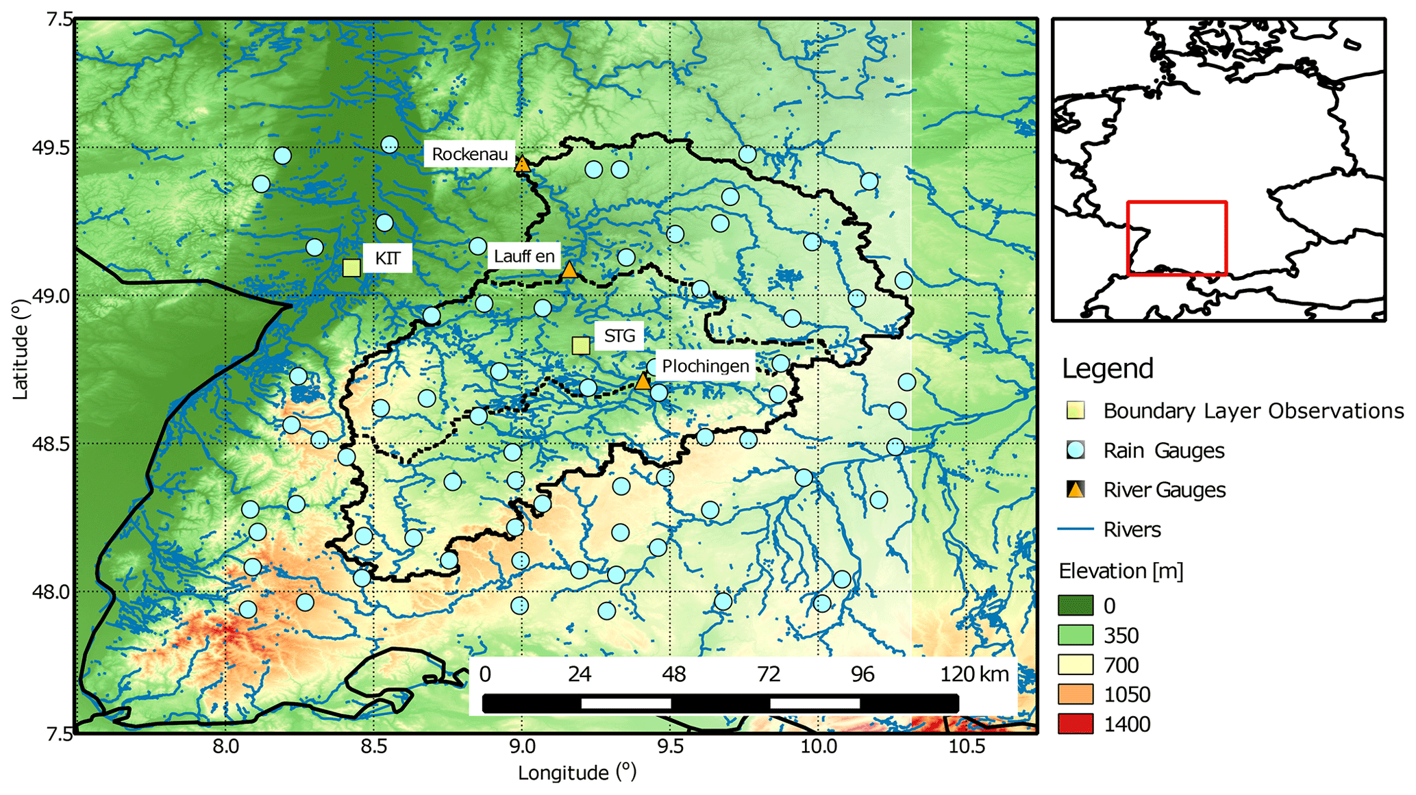
Figure 1 Location of the Neckar catchment within SW Germany.

The remainder of the paper is structured as follows. In Sect. 2, we introduce the simulation platform (TerrSysMP), while Sect. 3 describes in detail the surface and subsurface parameters for topography, soils and aquifers, land use, vegetation, and the river network. In Sect. 4, we show snapshots and time series of state variables or system parameters extracted from the simulated catchment and compare them to observations in the real Neckar catchment to demonstrate how well the most important requirements are met. These results as well as possible ways to improve them are discussed in Sect. 5, together with several issues which came up during the development phase. We provide conclusions and an outlook in Sect. 6.

2 The Terrestrial Systems Modeling Platform

We used the Terrestrial Systems Modeling Platform (TerrSysMP; see Shrestha et al., 2014; Gasper et al., 2014; Sulis et al., 2015) developed within the Transregional Collaborative Research Centre TR32 (Simmer et al., 2015) for the generation of the simulated catchment. TerrSysMP couples (Fig. 1 in Gasper et al., 2014) the hydrologic flow model ParFlow v693 (Ashby and Falgout, 1996; Jones and Woodward, 2001; Kollet and Maxwell, 2006), the land-surface Community Land Model (CLM) v3.5 (Oleson et al., 2008), and the atmospheric Consortium for Small-scale Modeling (COSMO v4.21, Baldauf et al., 2011) model via the Ocean Atmosphere Sea Ice Coupling framework (OASIS3) (e.g., Valcke, 2006) using a dynamical two-way approach including down- and upscaling algorithms for fluxes and state variables between computational grids of different resolutions.

ParFlow is a variably saturated watershed flow model which solves the three-dimensional Richards equation to model saturated and unsaturated flow in the subsurface and the fully integrated kinematic wave equation to model two-dimensional overland flow. Other global and regional hydrological models also use the latter to route overland flow, e.g., MODCOU (Haefliger et al., 2015) and TRIP (Alkama et al., 2012). Advanced Newton–Krylov multigrid solvers are used that are especially suitable for massively parallel computer environments. Excellent model performance and parallel efficiency have been documented by Jones and Woodward (2001), Kollet and Maxwell (2006), and Kollet et al. (2010). A unique feature of ParFlow is the use of an advanced octree data structure for rendering overlapping objects in 3-D space which facilitates modeling complex geology and heterogeneity as well as the representation of topography based on digital elevation models and watershed boundaries.

CLM is a single-column biogeophysical land-surface model released by the National Center for Atmospheric Research (NCAR) which considers coupled snow, soil, and vegetation processes. Land-surface heterogeneity is represented as a nested subgrid hierarchy in which grid cells are composed of multiple land units (glacier, lake, wetland, urban, and vegetation), snow/soil columns (to capture variability in snow and soil states within each land unit), and plant functional types (PFTs) to capture the biogeophysical and biogeochemical differences between broad categories of plants in terms of their functional characteristics. In TerrSysMP, the 1-D Richards equation model included in CLM is replaced by ParFlow.

COSMO is a limited-area non-hydrostatic numerical weather prediction model, which operationally runs at the German weather service (Deutscher Wetterdienst, DWD), among others, for numerical weather prediction (NWP) and various scientific applications on the meso-β and meso-γ scales. COSMO is based on the primitive thermo-hydrodynamical equations describing compressible flow in a moist atmosphere. As a limited-area model, COSMO needs lateral boundary conditions from a driving larger-scale model. We impose the lateral conditions by nesting COSMO in COSMO-DE, which spans Germany. At the lateral boundaries, a relaxation technique is used in which the internal model solution is nudged against an externally specified solution over a narrow transition zone between the two domains. Version 3.5 of CLM that is used here is already relatively old. Even though version 5 was not yet available when we started our work, it is now and comparison is warranted. Newer versions of CLM have several major improvements over v3.5. The first one is a more sophisticated routing scheme, leading to much improved soil moisture profiles. In our case, we replace this part with ParFlow anyway, so our older version is not a disadvantage in that regard. Other improvements are the inclusion of carbon and nitrogen cycles, as well as more options for crop type vegetation. Here, we purposely simplify our setup, as we not only have and want static land use but also use a blend type of crop with no sharp changes in leaf area index (LAI) due to harvests. Instead, we assume harvest to be an ongoing process all throughout autumn. Thus, all these improvements do not downgrade the simulation results presented and discussed in this study.

Within OASIS3, the upscaling algorithm uses the mosaic or explicit subgrid approach (Avissar and Pielke, 1989) in which high-resolution land-surface fluxes are averaged and transferred to the coarser resolution of the atmospheric model component. The implemented Schomburg scheme (Schomburg et al., 2010, 2012) downscales atmospheric variables of the lowest atmospheric model layer to the higher-resolved land-surface model. The scheme involves (i) spline interpolation while conserving mean and lateral gradients of the coarse field, (ii) deterministic downscaling rules to exploit empirical relationships between atmospheric variables and surface variables, and (iii) the addition of high-resolution variability (i.e., noise) in order to honor the non-deterministic part and to restore spatial variability.

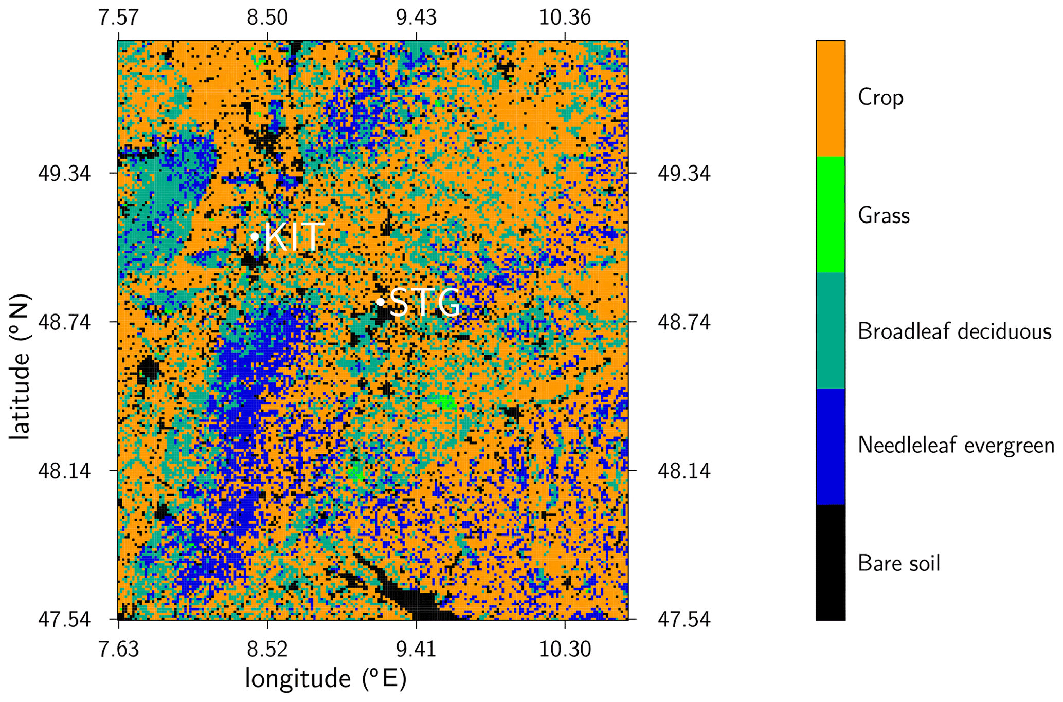
Figure 2 Land cover in the simulated domain covering the entire Neckar catchment and bounding areas. KIT: Karlsruhe Institute of Technology (location of meteorological tower observations), STG: Stuttgart (location of radiosonde observations).

TerrSysMP allows simulating the terrestrial water, energy, and biogeochemical cycles from the deeper subsurface including groundwater (ParFlow) across the land-surface (CLM) into the atmosphere (COSMO). Water and energy cycles are coupled via evaporation and plant transpiration; these processes are modeled by CLM with a non-linear coupling to ParFlow through soil-water availability and root-water uptake (Fig. 2). The two-way coupling between CLM and COSMO encompasses radiation exchange and turbulent exchanges of moisture, energy, and momentum. OASIS3 allows for different temporal and spatial resolutions of the coupled model components. For example, a temporal resolution of 15 min is sufficient for the subsurface and land-surface components, whereas time steps as small as 5 s are needed for the atmosphere. A higher spatial resolution can be assigned for the surface and subsurface parts to allow for a better representation of soil and land-use heterogeneity.

Since high-resolution and long time series of the fully coupled system are needed to satisfy our need to check the statistical behavior of the system, the models were run on the IBM/BlueGeneQ system JUQUEEN at the Jülich Supercomputing Centre (Jülich Supercomputing Centre, 2015). JUQUEEN has a total of 28 672 nodes with 16 cores each. Our configuration involved using 256 nodes for 12 h, restarting the simulation every 7 simulation days. This is necessary as the runtime for ParFlow can vary greatly depending on the conditions in the catchment. The total number of grid cells for the domain is 323 675 per model layer, with 10 layers for CLM and 50 layers for ParFlow, and 58 420 grid points for the 50 COSMO layers, resulting in 22.3 million grid cells. We ran the fully coupled model for a period of nine years (2007–2015) as 2007 was the first full year where high-resolution atmospheric forcings were available and 9 years was the maximum possible simulation length given constraints on compute resources. On average, the actual runtime was approximately 8 h. This means that for 1 year of simulation roughly 1.7 million core hours are needed. For the full 9-year time series, that is about 12 million core hours; another ∼8 million hours were needed for the spin-up. We used an output interval of 15 min, which results in a total output of 38.5 TB of data for the full time series, where about half was produced by COSMO and a quarter each by CLM and ParFlow.

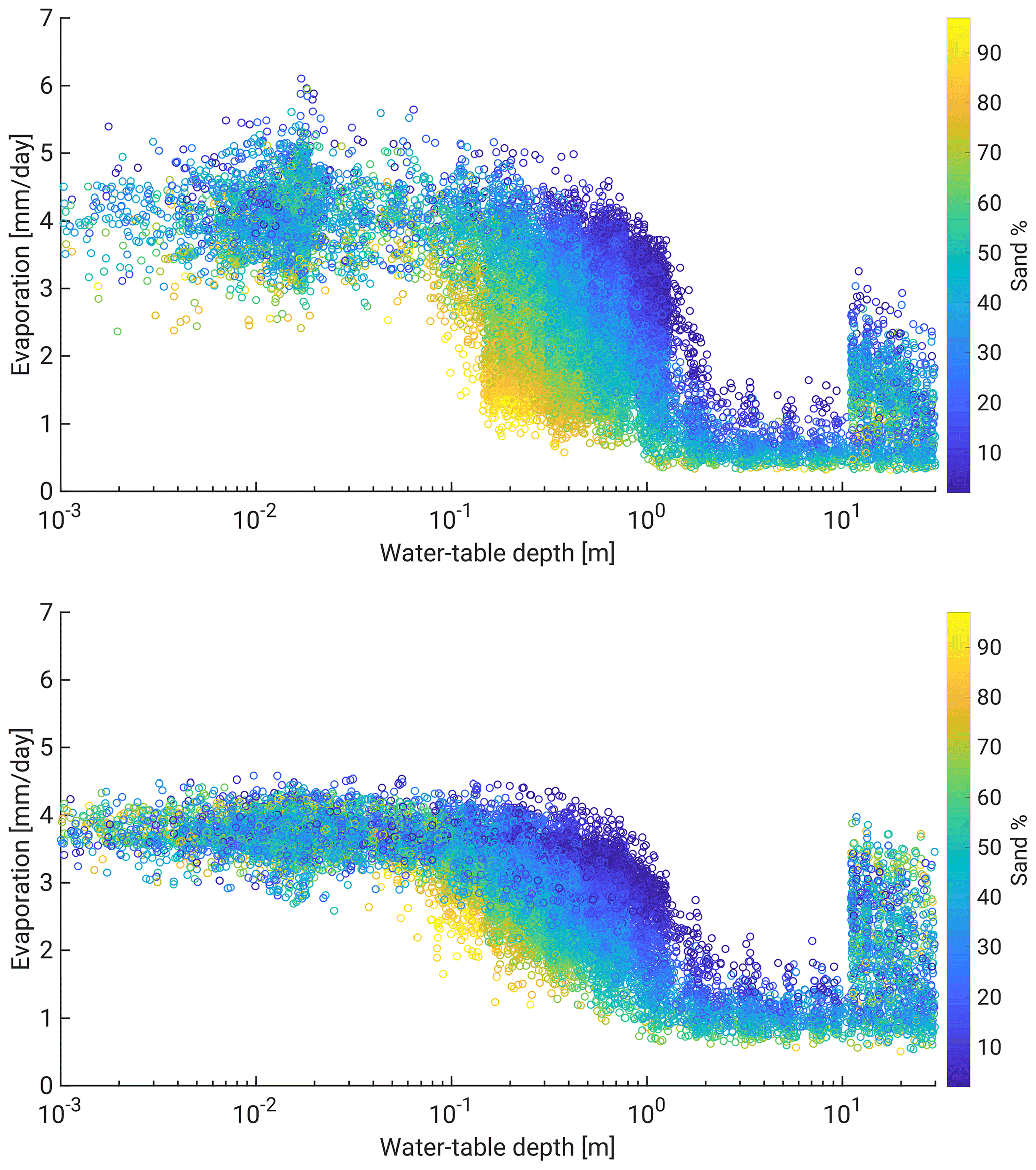
Figure 3 Daily average evaporation simulated for 30 April (too) and 31 July 2007 (bottom) in mm d⁻¹. The color indicates soil sand percentage.

3 Description of the virtual Neckar catchment

Our simulated catchment is based on the Neckar catchment in southwestern Germany (see Fig. 1), east of the Black Forest mountain range and north of the Jurassic ridge of the Swabian Alps. The catchment has a varying topography including mountains up to 1050 m a.s.l., river valleys, different land-use types, i.e., grassland, cropland (majority of the area), broadleaf and needle leaf forest (see Fig. 3), and relatively large soil spatial variability. Annual mean precipitation over the real catchment ranges between 500 and 2000 mm (see Sect. 5.1), with the highest values over the Black Forest. Interannual variability of precipitation can reach up to one-third of the mean value. Monthly precipitation can vary largely, and its mean annual cycle is weak with slightly lower values in spring and autumn. While summer precipitation is dominated by convection, winter precipitation is predominantly related to fronts of extratropical cyclones with enhanced precipitation over the mountains due to orographic lift. Daily average temperatures vary with altitude between −5 and 0 ^∘C in January and between 13 and 18 ^∘C in July. Land use and cover in the lower elevations are dominated by agriculture, while the Black Forest features mainly needleleaf trees. Broadleaf trees can be found over smaller areas throughout the catchment. The distance to groundwater is in large parts of the area restricted to a few meters, in particular in lowland areas, which assures strong coupling between the groundwater table and evapotranspiration (Maxwell et al., 2007). These typical central European catchment features in addition to the relatively shallow groundwater tables (implying a stronger possible feedback of groundwater on atmospheric conditions) were the basis to select the Neckar catchment for our simulation.

The computational domain is a rectangular area of ∼57 850 km² encompassing the Neckar catchment of ∼14 000 km². The domain is larger than the Neckar catchment in order to allow the atmospheric model to develop its own internal dynamics. COSMO is run on a 1.1 km horizonal grid with 230×254 grid points, which includes a four-grid-point-wide outer frame zone where only the lateral boundary forcing is used without coupling to the CLM, as well as 50 vertical layers in hybrid coordinates (terrain following at the surface, flat in the stratosphere). COSMO is set up identical to the operational COSMO-DE setup of the German national weather service (DWD); e.g., the deep convection parameterization is switched off because at the chosen grid resolution convection is enabled by the dynamical core (see Sect. 2.1). In COSMO-DE, the operational resolution is 2.8 km, so that the approximation regarding deep convection is even more appropriate in our simulations. Similar choices were taken by Smith et al. (2015), who simulated precipitation events of roughly the same domain using nested WRF models, where the cumulus parameterization was switched off at horizontal resolutions of 900 and 300 m. Lateral boundary forcing and constant fields (topography, land mask, etc.) are provided by the COSMO-DE analysis fields, which are downscaled to the 1.1 km grid by linear interpolation. The lateral relaxation zone, which moderates the jump from the lateral driving fields to the inner model area, is set to 12 km.

A software restriction (unfixable bug specific to the supercomputing system we were using for our simulation runs as described in the previous section) did not allow for cases with more than 4.2 million CLM columns, as the model did not initialize properly and crashed, implying that a higher spatial resolution for CLM and ParFlow than 400 m could not be achieved for the Neckar catchment on the used system. So, ParFlow and CLM use the same horizontal grid with a resolution of 400 m and 535×605 grid points. The vertical grid for both component models is partially the same, with CLM limited to 10 vertical layers up to a total depth of 3 m shared with ParFlow, which has in total 50 vertical layers reaching down to 100 m. COSMO runs with a 5 s time step, while CLM and ParFlow run at 15 min time steps, which is also the coupling frequency.

For setting up CLM, the European digital elevation model (DEM) by the European Environment Agency (EEA) (http://www.eea.europa.eu/data-and-maps/data/eu-dem, last access: 1 October 2017) was projected to the latitude–longitude grid and bi-linearly interpolated to 400 m from the original 30 m spatial resolution. The same DEM is used to create the slope input files for ParFlow. A slight modification to the original DEM was made in order to ensure that the simulated Neckar River would flow in the correct valley, especially in the upper half of the catchment where the valley is not always properly resolved by the 400 m resolution. In total, the elevation of eight grid points was reduced to achieve proper routing for the Neckar River. The resulting elevation map is part of the CLM input data and is available with the dataset as supplementary material (https://cera-www.dkrz.de/WDCC/ui/cerasearch/entry?acronym=Neckar_VCS_v1_FORCING, last access: 9 August 2021). We have not considered rivers outside the Neckar catchment in these corrections; thus, there are cases where their routing is not identical to the real rivers.

Land use is taken from the 2006 CORINE Land Cover Data Set (https://land.copernicus.eu/pan-european/corine-land-cover/clc-2006, last access: 29 July 2021) also provided by EEA. Since the latter dataset features many more land-use types (at a resolution of 100 m) than required by CLM, they were grouped according to the CLM (International Geosphere-Biosphere Programme, IGBP) plant functional type classes (1) broadleaf forests, (2) needleleaf forests, (3) grassland, (4) cropland, and (5) bare soil. Urban areas are not considered in this setup and replaced by bare soil. Water surfaces (e.g., larger lakes like Lake Constance in the south of the domain) are also treated as bare soil in CLM, while COSMO uses its own land mask and specific calculations for water surfaces. Therefore, no values from CLM are used for water surfaces in COSMO. A few hundred grid cells feature shrubs (mostly areas that are re- or deforested or areas at higher altitudes) which are treated as forests, and each grid cell features only one – the most dominant – plant functional type. The plant LAI is computed from MODIS (Myneni et al., 2002) as monthly averages for the year 2008 for each of the four vegetated land-use classes. As a result, interannual variability is not considered in this simulation, as we have the same LAI curve for each PFT each year. This somewhat limits the comparability to ET observations especially in spring. This LAI is increased for all plant functional types by 20 % on average (more for forests and less for grassland and crops) in the summer months and significantly changed from factors of less than 1 to 3.3 in wintertime (DJF average) for needleleaf forests in order to account for known biases in the MODIS data (Tian et al., 2004). This is mostly related to snow cover and fractional land cover due to the satellite footprint which often includes other vegetation types or roads and other buildings, leading to an underestimation for a grid cell that is fully covered by just one type as we have used. The stem area index (SAI) is estimated from the LAI by a slightly modified (no dead leaves for crops, constant base SAI of 10 % of the maximum LAI) formulation of Lawrence and Chase (2007) and Zeng et al. (2002) to better represent European tree types. Vegetation height was set to 7 m for needleleaf trees and 10 m for broadleaf trees to account for partial coverage by shrubs, to 20–120 cm for crops, and to 10–60 cm for grass depending on the time of the year with low values in the winter months and largest values in July and August. Since we consider only one crop type, we do not specify a harvest date when the plant height drops to its minimum but assume a smooth decline between August and October.

For the representation of soils in CLM, we use the 1:1 000 000 soil map (BUEK1000, roughly 1 km resolution) provided by the Federal Institute for Geosciences and Natural Resources (BGR) (http://www.bgr.bund.de/DE/Themen/Boden/Informationsgrundlagen/Bodenkundliche_Karten_Datenbanken/BUEK1000/buek1000_node.html, last access: last access: 29 July 2021). This soil map is available for all of Germany; thus, only small areas in Switzerland and France are missing outside the Neckar catchment for which we assume a nearby soil class. BUEK1000 offers sand and clay percentages as well as carbon content for two to seven soil horizons down to a maximum depth of 3 m for each soil type. The carbon content is used to infer soil color. For urban areas (modeled as bare soil, as mentioned above) a fixed soil color (class 8 in CLM) was used.

Since soil properties may vary substantially at scales smaller than the 1 km for which BUEK1000 is appropriate, which might impact system dynamics (Binley et al., 1989; Herbst et al., 2006; Rawls, 1983), the soil map is downscaled by artificially adding variability using the conditional points method recently presented in Baroni et al. (2017) as follows:

1. The BUEK1000 soil map is randomly sampled at 1995 point locations with one sample every 5 km² on average, a minimum sample distance of 250 m, and at least one sample for each soil type of the original soil map, which is realistic in the context of how soil maps are usually created. This strategy resulted from extensive testing by minimizing the tradeoffs between reproducing the main features of the original soil map and creating variability at finer resolution.

2. The sample locations are used as conditional points for further interpolation. Here, texture, carbon content, and depth of the first three soil horizons are extracted from the BUEK1000, resulting in variable soil depth rather than the assumed unrealistic uniform soil depth. In addition, the sand content of the original map was increased by 20 % (except for areas with very high sand content to avoid grid cells with >90 % sand), resulting in a slightly higher hydraulic conductivity because previous simulations yielded too-shallow unsaturated zones related to the spatial resolution of the simulation. Changing sand content increased the thickness of unsaturated zones and lowered groundwater tables, fixing most of the emerging biases.

3. Experimental variograms and cross-variograms are calculated for all variables, and exponential models were fitted to all spatial structures.

4. A texture map (sand and clay percentage) is generated using a single realization based on conditional co-simulation (Gomez-Hernandez et al., 1993) to provide the subscale variability (<1 km²). Soil horizon depths and carbon content are, however, assumed to have a smoothed spatial variability; therefore, they are interpolated based on ordinary kriging as the removal of small-scale variability is not important for the depth and carbon content.

5. Since ParFlow describes retention and hydraulic conductivity curves based on Mualem–van Genuchten parameters, pedotransfer functions are applied to estimate these parameters. The pedotransfer function of Cosby et al. (1984) is used to estimate saturated hydraulic conductivity based on soil texture, the one from Rawls (1983) is used to estimate soil bulk density based on soil texture and organic matter, and the one from Tóth et al. (2015) is used to estimate van Genuchten parameters based on soil texture and bulk density. These have been selected based on data availability, applicability of the particular approaches, and previous evaluations conducted in the area (Tietje and Hennings, 1996).

In order to keep soil porosity identical between CLM and ParFlow, we replaced the porosity calculation within CLM (which uses a different pedotransfer function). The Manning's surface roughness was set to a constant value of $\mathrm{5.52}\times {\mathrm{10}}^{-\mathrm{4}}$ h m${}^{-\mathrm{1}/\mathrm{3}}$ and the specific storage to $\mathrm{1}\times {\mathrm{10}}^{-\mathrm{3}}$. The chosen surface roughness value results in a realistic base flow for the local rivers without calibration. Repercussions of this choice are discussed in Sect. 6. Slopes of the main rivers are additionally smoothed to avoid artificial ponded areas.

All these changes are part of the forcing files that are provided with the full dataset, making it easy to reproduce our simulations (https://cera-www.dkrz.de/WDCC/ui/cerasearch/entry?acronym=Neckar_VCS_v1_FORCING, last access: 29 July 2021).

In order to allow for realistic flow in the saturated zone, the 3-D geologic model of the geological survey of the state of Baden-Württemberg was used from which 11 rock types were defined for Baden-Württemberg (see Fig. A1). Some characteristic features of the domain, such as middle Triassic and Jurassic karst aquifers, are not included to avoid the manifold hydrological challenges related to its modeling. While this can have a significant impact on groundwater representation in the karst areas, for the rather short time period considered here, we expect a limited impact on near-surface soil moisture content as the affected areas have in general deeper groundwater levels. For areas outside of Baden-Württemberg, we extended the rock types at the boundary outwards to cover the full computational domain. Table 1 summarizes porosity and hydraulic conductivity used in the domain for the different stratigraphic units. Since karst features of limestones are not considered, porosities in stratigraphic units containing limestones and crystalline rocks are set considerably higher than in nature to somewhat counter this.

Not covered by the discussed datasets (not part of the soil and not large enough to be resolved in the geological map) are the large alluvial bodies filling large part of the Neckar valley throughout the domain (Riva et al., 2006). Up to 30 % of the runoff takes place in the subsurface, especially during periods of base flow, according to a subcatchment simulation performed for the year 2007. In that simulation, we used measured precipitation and river discharge data together with the simulated evapotranspiration to calculate the water balance over a whole year. While our simulated evapotranspiration rates may be inaccurate, it is implausible that this can account for 30 % of the precipitation, as in this climate we are almost always energy limited, and therefore ET errors will be smaller and mostly related to errors in atmospheric forcings and LAI. This implies that the water could only have left the domain through the subsurface. Thus, gravel channels are needed to account for this lateral flow. Since the valleys in the catchment are often small compared to the limited horizontal resolution of the model, we conceptualize the alluvial bodies as gravel layers underneath all river cells (cells with a mean pressure head >0.1 m) and directly next to rivers (riverbanks, i.e., one grid point besides each river cell). The assumed gravel layers reach from beneath the soil down to a depth of 8 m. The gravel cells are parameterized with a high hydraulic conductivity of 1 m h⁻¹, a porosity of 0.6 and van Genuchten parameters of 2 for n and 4 m⁻¹ for α (residual saturation is 0.06 cm³ cm⁻³). Our setup results in a reasonable distribution of surface and subsurface discharge at the outlet of the catchment and reasonable river–aquifer exchange fluxes. In addition to the gravel channels, we included a layer of weathered bedrock, which starts below the soil and extends down to a depth of 6 m. This layer is characterized by substantially larger porosity (0.4) and hydraulic conductivity (0.1 m h⁻¹) than the rock below. This layer was added to enhance subsurface flow and counter the common occurrence of too-shallow water levels if these features are not included. Both these changes are realistic when compared to the actual morphology of the Neckar river valley. While it is quite narrow in many places, there are still significant alluvial deposits everywhere except the furthest upstream region (which are not considered for this anyway due to the pressure cutoff). The choice for the weathered bedrock layer is also reasonable given the temperature and moisture ranges leading to imperfections in the rock layers near the surface.

Since we enforce no-flow boundary conditions at the subsurface domain boundaries, all water has to eventually reach the surface in order to leave the domain. This happens predominantly in areas outside of the Neckar catchment, e.g., in the upper Rhine Valley; thus, soil moisture values in this region may be too high.

4 Results

In the following, we present example results of the simulated-reality simulations in order to demonstrate its potential for a better understanding of the dynamics in coupled terrestrial systems. We will also show that the simulations quite well resemble observations in the real Neckar catchment, and thus can be used to develop and evaluate modeling and prediction strategies. Precipitation is the strongest hydrological driver in this region; thus, its realistic spatial and temporal variability in the domain including its statistical relations with topography is important. Also, the state of the atmospheric boundary layer, which reflects the interaction of the land surface with the atmosphere, is a critical component of the terrestrial system, which should be represented by the simulation with some confidence. Along with the comparisons, we will also discuss the challenges experienced with such a modeling setup.

Even though we do not aim to be as close to reality as possible, we feel it is important to show that the model system is behaving as expected and is thus suitable for the various use cases we discussed. Figure A2 shows as an example result a snapshot of the simulated three-dimensional distribution of cloud water/ice, precipitation density, and volumetric soil moisture. The soil exhibits different soil moisture layers, the variability of which is mainly connected to different soil hydraulic properties. Only clouds reaching high enough to have sufficient cloud ice produce precipitation, and some precipitation evaporates before it reaches the ground. Extended weather fronts moving through the domain (not shown), which are imposed by the boundary conditions, are also simulated realistically (timing, strength of wind gusts, change of wind direction, change in temperature and pressure) given the resolution of the atmospheric model.

4.1 Relation between water table depth and evapotranspiration

An important measure for hydrometeorological interactions within a catchment is the relation between water availability and surface energy flux partitioning. Thus, the simulated catchment should capture the expected reduced evapotranspiration (ET) with increasing distance to groundwater (e.g., Maxwell et al., 2007; Shrestha et al., 2014). In Fig. 3, we show daily averaged evaporation (which here is equal to ET as all other contributors are zero) values over bare soil against distance to groundwater for 30 April and 31 July for the year 2007. These days were chosen as they were preceded with several dry days in almost the whole catchment, leading to comparable states for the upper soil layers. April was almost completely dry (on average less than 3 mm precipitation over the domain), while July was much wetter, but the increased solar radiation and thus temperatures compared to April result in higher evaporation rates and thus a quicker drying of the top layer of the soil. Figure 3 indicates a reduction in evaporation when the distance to groundwater falls below 15–100 cm, depending on soil properties with faster evaporation reduction for increasing soil sand content. Such relations are less obvious for cells with significant plant cover: while trees show overall higher evaporation and almost no change with distance to groundwater due to their deep root zones, variability increases with larger distances to groundwater (not shown). Also crops and grassland show limited evaporation changes as a function of distance to groundwater, which can, however, be explained by the high water availability (no water stress) in the time period considered. Figure 3 also contains a small number of grid points at a water table depth of 7 m or deeper, with evaporation rates only slightly lower than in the shallow water table regions. These relate most likely to cells that retain high levels of upper-level soil moisture even during dry periods to support higher evaporation. This could be due to the way the water table is calculated. We define the water table as the deepest threshold between positive and negative pressure. Since there are some places where there is another saturated region closer to the surface, leading to higher water availability near the surface, the high value for the water table can be misleading with respect to near-surface soil moisture. Such a feature will only occur if the water table is deep enough to begin with, which is why we do not see this for water tables of less than 10 m. As a result, volumetric soil moisture for these cells with deep water table but high evaporation is much more similar to cells with a shallow water table than to cells with a deep water table but low evaporation.

We want to point out that in this region ET is almost always limited by atmospheric demand, which is why we limit the analysis to bare-soil evaporation only. Since the uppermost layers can dry quickly, the resulting drop in evaporation can be seen, which is not the case for ET if there is an extended root zone as we have for crops, grassland and forests. These bare-soil areas are not a feature of the real catchment and as such cannot be compared to real measurements.

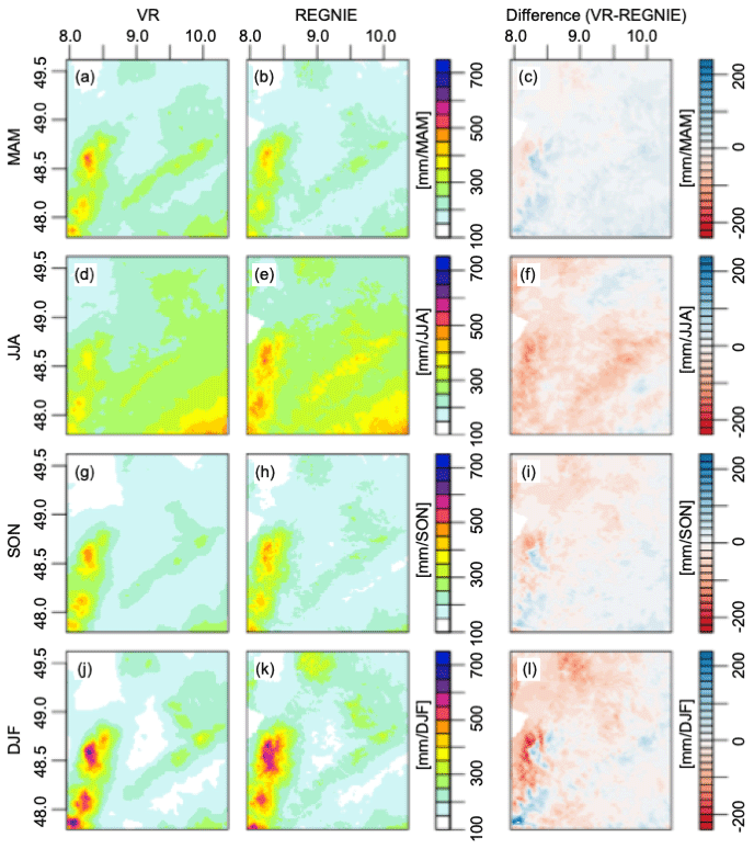
Figure 4 Mean seasonal precipitation over the Neckar catchment between 2007–2013 in the simulated reality (VR, left column) compared to the REGNIE dataset (middle column). The difference between VR and REGNIE is shown in the right column. Panels (a)–(c) show the comparison for spring (March–May); (d)–(f) for summer (June–August); (g)–(i) for fall (September–November); and (j)–(l) for winter (December–February).

4.2 Precipitation

We compare the simulated precipitation with the 1×1 km gridded REGNIE (Regionalisierung der Niederschlagshöhen) product of DWD, derived from in situ precipitation observations (Rauthe et al., 2013). For the evaluation of seasonal daily precipitation cycles, hourly observations of 71 DWD observational stations are used. The simulated seasonal mean precipitation (Fig. 5) and the annual mean precipitation (not shown) are governed by the orographic structures of the Black Forest and Swabian Alps. Values range between approximately 520 mm yr⁻¹ around Mannheim and 2105 mm yr⁻¹ over the Black Forest in good accordance with REGNIE concerning the overall pattern and range (510–2130 mm yr⁻¹). Overall, the simulation shows about 10 % higher annual precipitation in the east and south and about 25 % lower in the north and west compared to REGNIE. During winter (December to February), precipitation is dominated by advection from the west, which results in maxima over the upwind and peak zones of the mountains and leeward minima. The simulated winter pattern (j) compares well with REGNIE (k), but the model underestimates precipitation in the northwestern part of the catchment (l). Over the mountains, a slight lateral shift of this kind of precipitation pattern results in neighboring areas with under- and overestimation also found for COSMO simulations coupled to its own TERRA land-surface model (e.g., Dierer et al., 2009; Lindau and Simmer, 2013). In fall, the difference pattern between simulations and REGNIE (i) is similar to the winter pattern but has smaller contrasts. In spring, the simulated precipitation is higher compared to REGNIE. In the summer (June to August), cloud bases are usually higher and reduce the patterns caused by the luff–lee effects. Moist air extends further to the east and south and gets staunched by the alpine upland, leading to enhanced precipitation there. The simulated summer precipitation pattern, which is dominated by convective precipitation, resembles the REGNIE pattern but exceeds the latter by being 20 % lower over large parts of the catchment (Fig. 4).

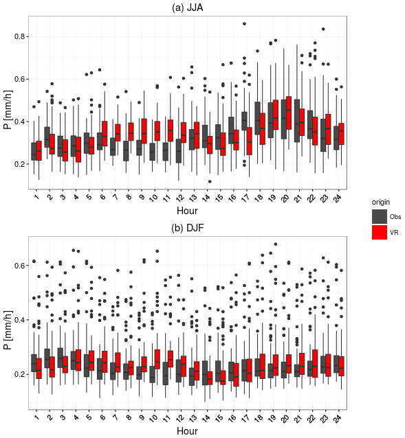
Figure 5 Mean diurnal precipitation cycle for the 71 DWD stations and the corresponding simulations for wet days (more than 1 mm d⁻¹) for June–August (a) and December–February (b) seasons. The upper and lower hinges correspond to the first and third quartiles, the center black line indicates the median, the upper whisker (analog for lower whisker) extends from the hinge to the highest value within 1.5 ⋅ (interquartile range), and the black dots mark the outliers.

The mean seasonal diurnal precipitation cycles (Fig. 5) reflect the dominating precipitation types. While observed and simulated winter precipitation (Fig. 5b) do not show a diurnal cycle, summer precipitation (Fig. 5a) increases over the afternoon reaching a maximum at about 19:00 LT in accordance with the maximum of convective precipitation. The simulations reproduce this pattern but exhibit a weak second peak between 06:00 and 12:00 LT while the afternoon–evening increase is delayed by about 2 h. The simulated daily precipitation distribution fits the observations especially in late afternoon and night, while it overestimates precipitation during the late morning and underestimates it in early afternoon in summer. In winter, this effect is much less pronounced. This behavior is related to the representation of convective showers in the atmospheric model. The responsible parametrization was not designed for the kilometer scale and application at this resolution results in a too-early onset of convective precipitation. While the simulated catchment has somewhat fewer dry and low precipitation days than REGNIE, the number of days between 4 and 10 mm are higher than in REGNIE (not shown). The simulated and observed seasonal precipitation cycles (Fig. 6) compare very well, and mean precipitation is nearly identical between simulations and observations. The model reproduces the seasonal cycle of maximum daily precipitation well, however with larger differences in the summer (see also Dierer et al., 2009).

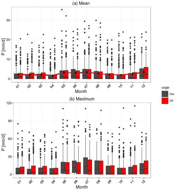
Figure 6 (a) Daily precipitation distribution on a monthly basis as observed (black) and simulated (red). The gray and red lines indicate the monthly mean precipitation. (b) Maximum daily precipitation for the given months for the 71 DWD stations and the corresponding simulation. Box sizes as explained in the caption of Fig. 10.

4.3 Atmospheric state variables and surface radiation

We compare the atmospheric boundary layer (ABL) of the simulated catchment to observations from the meteorological tower at Karlsruhe Institute of Technology (KIT; Kalthoff and Vogel, 1992) and with DWD radiosonde observations in Stuttgart (STG) (see Fig. 1 for locations and Table A1 for details of observed quantities). To avoid a biased comparison related to land-cover mismatches between the simulation and the actual land use at the observation sites, the simulation results are averaged over five-by-five atmospheric grid boxes centered around the observation sites, thus giving approximately the same fractional land cover as is present at the observation location.

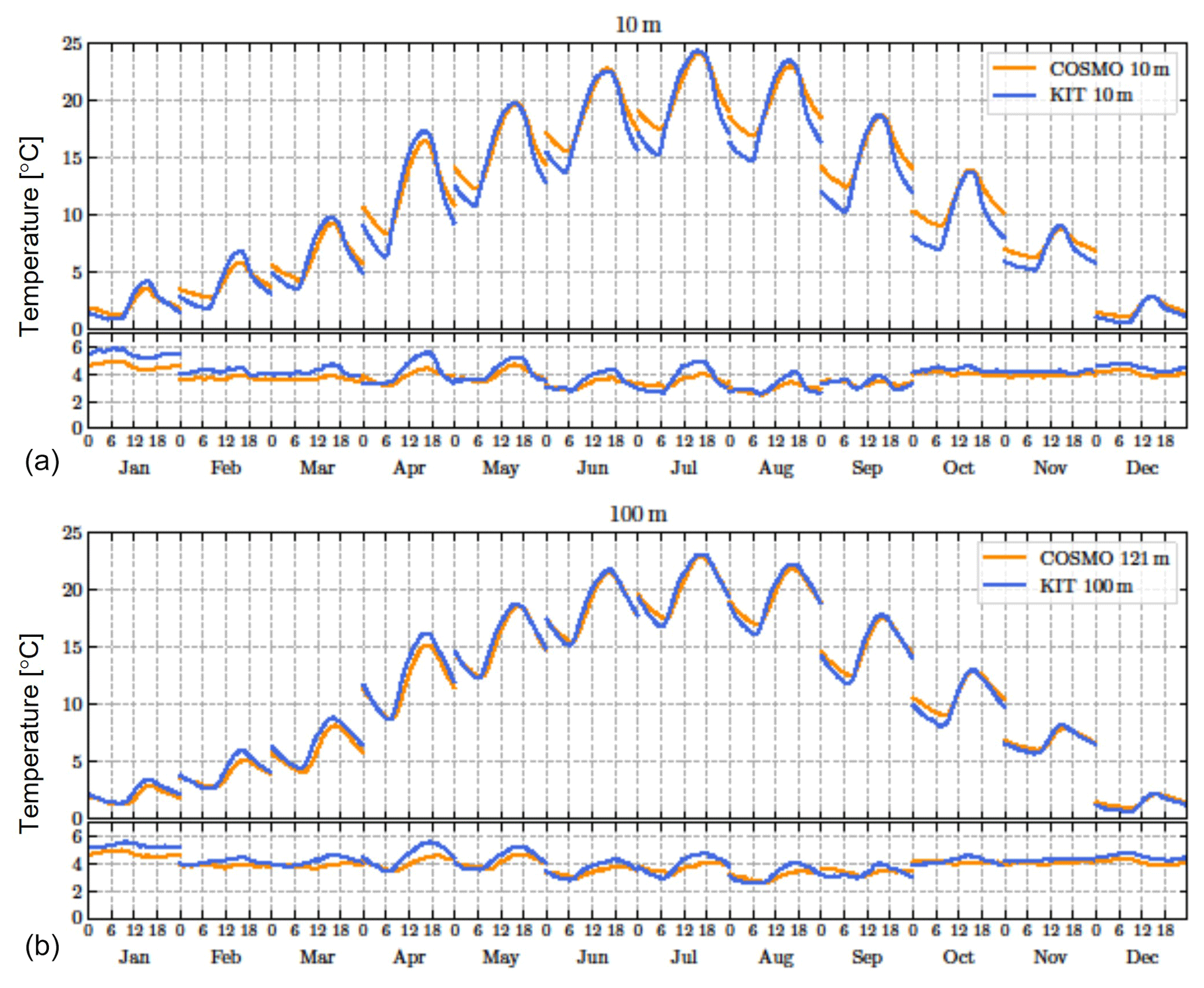
Figure 7 Monthly mean diurnal cycles (local time) and respective standard deviation (see text) for air temperature (^∘C) in 10 m (a) and 100 m (b) height at the KIT tower and for the COSMO grid boxes around the KIT location.

The 10 m mean diurnal minimum temperatures in the catchment are between 0.5 K (January) and 2.5 K (August) higher than observed (Fig. 7, top) and are reached approximately 1 h later than observed with the subsequent morning temperature rise shifted accordingly. The simulated diurnal temperature maxima are on average 0.7 K lower than in the observations and are reached 30 min later than measured. The morning temperature gradient in the simulation ranges from 0.10 K h⁻¹ in December to 0.31 K h⁻¹ in April, which compares reasonably well with the observations (0.13/0.52 K h⁻¹ in January/April). The evening cooling, however, progresses too slowly and results in too-high minimum temperatures. At 100 m above the ground, diurnal maximum temperatures agree within 0.7 K, while the warm bias of diurnal minimum temperatures (0.9 K) is smaller than at 10 m height (Fig. 7, bottom). Also at 100 m, a 1 h shift between the diurnal minimum temperatures and the morning temperature rise is found. At a height of 200 m, the simulated monthly mean diurnal cycles are practically identical to the KIT observations (not shown). The simulated temperature standard deviations (mean absolute difference for each time of day between the specific daily value and the corresponding monthly mean; see Appendix Eq. (A1) for details) are somewhat smaller than observed, especially in afternoons in the summer half year with underestimations of the temperature standard deviation larger than 20 %.

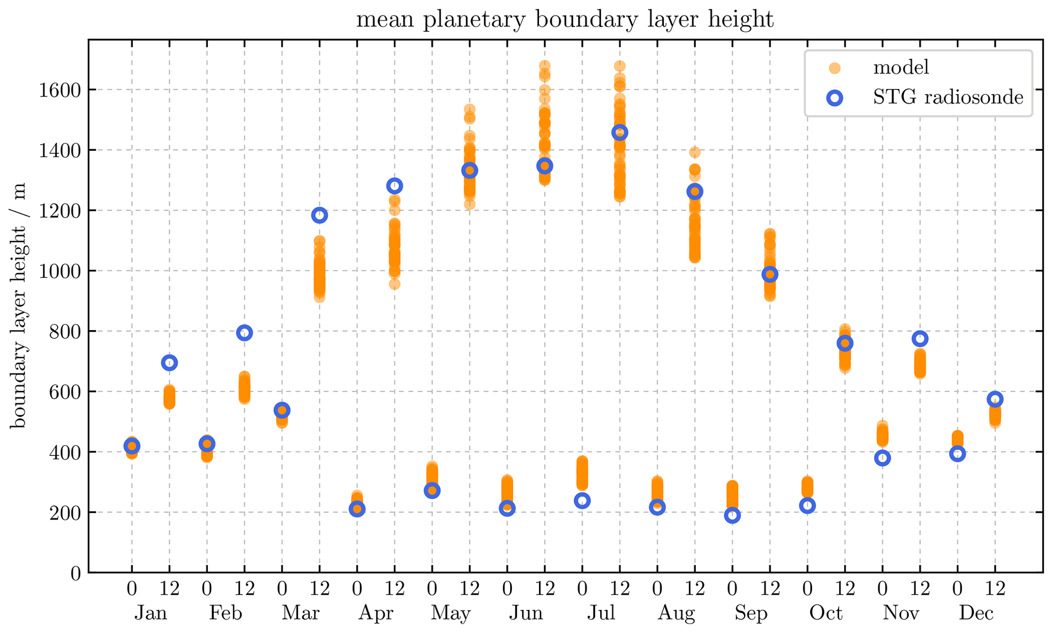
Figure 8 Monthly mean boundary-layer height at 00:00 and 12:00 LT for different land covers diagnosed from radiosonde observations at STG and from atmospheric profiles above grid boxes of CLM.

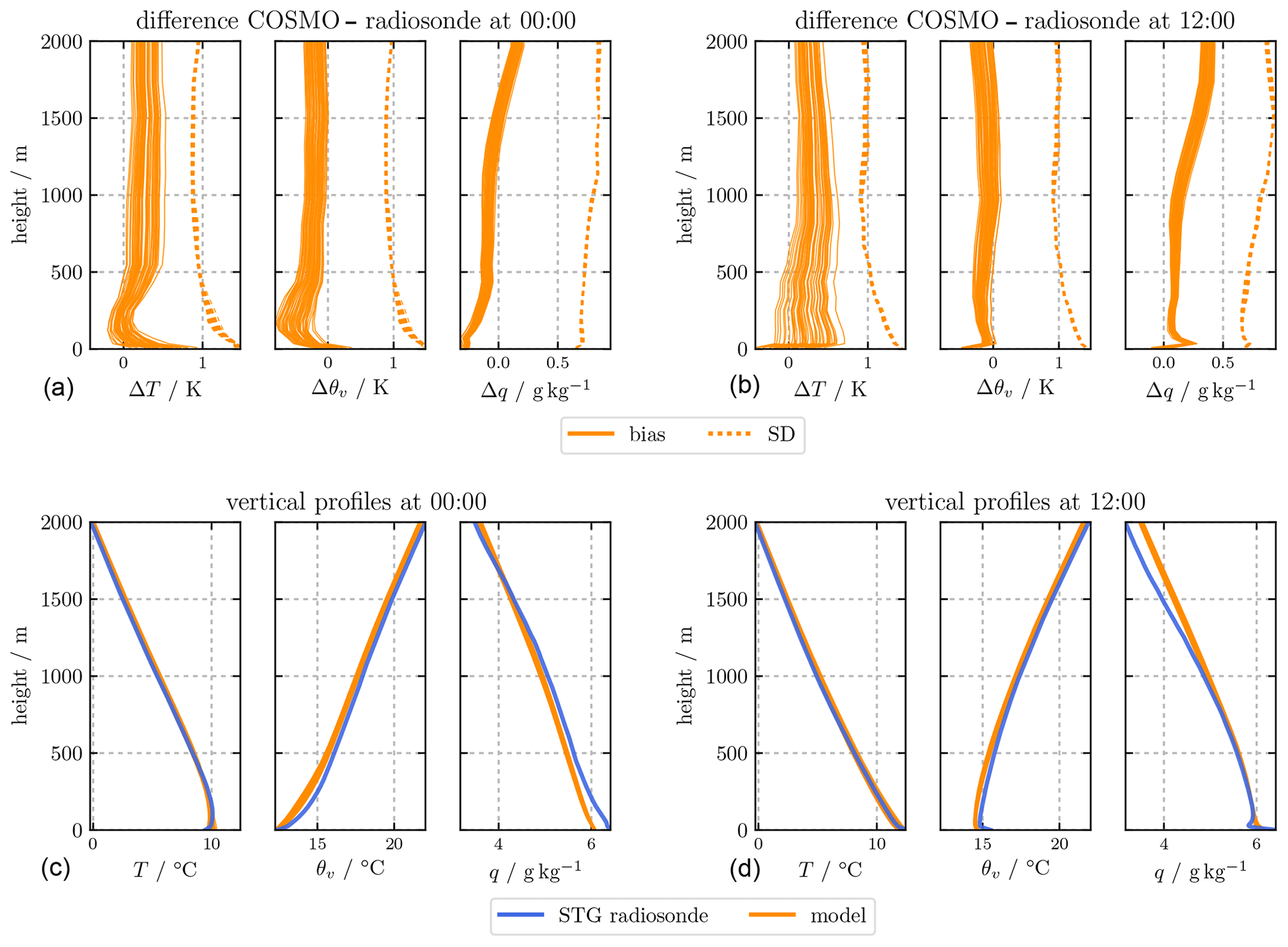
Figure 9 Mean vertical profiles of temperature, virtual potential temperature, and specific humidity (a, b), and mean differences between modeled and observed data including the standard deviation of the differences (c, d). The experimental data are from the radiosonde data at STG and the simulated data from the grid boxes of the simulated catchment with different land cover (a, c: 00:00 LT, b, d: 12:00 LT).

COSMO in TerrSysMP estimates ABL heights via the bulk Richardson number criterion with a threshold of 0.22 for unstable and 0.33 for stable conditions (Szintai and Kaufmann, 2008). Both seasonal and diurnal variations of the mean ABL height at 00:00 and 12:00 LT agree well with the observations using the same criterion (Fig. 8), but the simulation tends to overestimate ABL heights during nighttime by up to 150 m and underestimate it during daytime by up to 200 m in March. Figure 9 compares simulated mean vertical profiles of temperature, virtual potential temperature, and specific humidity with radiosonde observations at 00:00 and 12:00 LT in STG including the mean differences (bias) and the standard deviation of the differences. Simulations are up to 0.9 K warmer close to the surface at 00:00 LT and up to 0.5 K colder at 12:00 LT. At larger heights, the simulations are up to 0.5 K warmer depending on land cover. Specific humidity profiles at 00:00 LT are approximately 0.2 g kg⁻¹ too dry close to the surface and 0.2 g kg⁻¹ too wet above 1500 m. At 12:00 LT, profiles are up to 0.3 g kg⁻¹ too wet throughout. The simulations have smaller virtual potential temperature gradients and are thus less stable close to the surface at 00:00 LT. At 12:00 LT, the decreasing virtual potential temperature close to the surface is not captured and tends towards a more neutral instead of unstable profile at low heights.

At KIT (STG), the land surface receives on average 20 W m⁻² (5.3 W m⁻²) more incoming shortwave radiation and 18 W m⁻² (8 W m⁻²) less incoming longwave radiation indicating a somewhat lower cloud cover (or lower cloud optical depth) as observed. During daytime (06:00–22:00 LT), the mean outgoing longwave radiation matches the KIT observations, while at nighttime (22:00–06:00 LT) values are 7.2 W m⁻² larger than observed, which corresponds to a higher surface temperature of approximately 1.4 K.

Overall, the atmospheric profiles, including the ABL heights, are very close to observations during the day and at heights above 10 m. Noteworthy differences only occur close to the surface with too-high nighttime temperatures (up to 2.5 K in summer) and subsequently too-small morning temperature gradients. Somewhat higher incoming shortwave and lower incoming longwave radiation at the surface indicate less cloud cover (or lower cloud optical depths) compared to the observations. These results are in line with a previous evaluation of a 2.2 km COSMO simulation (Ban et al., 2014). In addition, we note somewhat reduced unstable conditions at daytime close to the surface in the simulations.

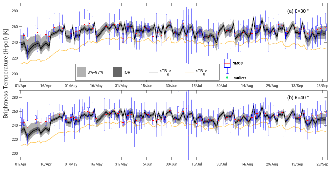
Figure 10 Area-averaged L-band brightness temperature the period from April to September 2011 for an incidence angle of 30^∘ (a) and 40^∘ (b). The boxplots indicate the real SMOS observations averaged over the same domain. The black line is the median of the observations simulated with CMEM. The dark gray area corresponds to the interquartile range (IQR), while the light gray area encompasses the 3 % to 97 % range. The continuous orange line indicates the brightness temperature without taking into account an assumed bias in surface soil moisture content (see text).

Figure 11 Hourly values river discharge at the gauging stations – Rockenau (P1), Lauffen (P2) and Plochingen (P3) – for the year 2007. Blue: observed; red: simulated catchment.

4.4 Passive microwave observations

The most direct area-covering observations of soil moisture are currently provided by L-band (1.4 GHz) passive microwave observations from satellites. The Community Microwave Emission Model (CMEM) is used as a forward operator to simulate the brightness temperatures (TB) at this frequency in vertical and horizontal polarization (de Rosnay et al., 2009). CMEM simulates brightness temperatures at the top of the atmosphere resulting from microwave emission and interaction by soil, vegetation, and atmosphere based on the state variables of the simulated catchment. Input to CMEM are the percentages of clay and sand in the soil, the coverage with open water surfaces, the profiles of soil moisture and soil temperature, vegetation types, and LAI. Satellite orbit geometry, antenna pattern, footprint, and incidence angle are taken into account following the ESA Soil Moisture and Ocean Salinity (SMOS) instrument specifications; i.e., a full-width-half-maximum field of view leading to a footprint of 40 km across orbit and 47 km along orbit at multiple incidence angles (Kerr et al., 2001) is applied. This antenna pattern weighs the grid-cell-simulated brightness temperatures (Fig. 11, left) in order to obtain simulated SMOS observations. Finally, these synthetic observations are rendered according to pixels based on the icosahedral Snyder equal area (ISEA) projection at a spatial separation of about 15 km similar to the SMOS L1C TB data product (Fig. A4, right), which can then be compared with observations for an indirect evaluation of the simulation. Every pixel corresponds to a fixed geolocation of the real SMOS L1C data product over the modeled area. Optionally, the satellite observation operator in TerrSysMP is able to also replicate the NASA SMAP (Soil Moisture Active Passive) radiometer (Saavedra et al., 2016) for years beyond 2015 (since the time SMAP data have been available).

We evaluate the simulated brightness temperature distribution over the domain with real SMOS observations between April 2011 and September 2011. The SMOS observations are corrected from radio-frequency interference (RFI) effects over the region following Saavedra et al. (2016). Initial results with CMEM-adapted parameters for surface roughness and vegetation optical thickness (which needed to be increased from its standard values found in the literature) lead to a systematic underestimation of the brightness temperature of about −20 K on average (see orange line in Fig. A3, which compares real SMOS observations with the simulated brightness temperatures) and maximum and minimum differences of −33 and −6 K, respectively, for an incidence angle of 30^∘. A similar underestimation of −14 K resulted for the 40^∘ incidence angle with maximum and minimum values of −34 and +15 K (lower plot in Fig. 10). Those differences are mainly caused by the too-large near-surface soil moisture values in the simulated catchment. The cumulative distribution functions of the satellite-derived soil moisture products and the simulated soil moisture suggests an about 63 % higher near-surface soil moisture compared to the satellite estimates (Saavedra et al., 2016, Fig. 6) with extremes of 44 % and 95 %. With that, a daily matching of the cumulative distribution functions of the simulated catchment and satellite retrieved soil moisture is performed to find a factor which then is assumed to be the soil moisture bias of the simulation and is applied as a correction factor. Figure 10 compares true SMOS observations with simulated brightness temperatures obtained without and with day-to-day correction for the assumed soil moisture bias of the simulation. The correction decreases the average bias in brightness temperature from −20 K (−14 K) to about −3 K (−2 K) for the incidence angle of 30^∘ (40^∘) at horizontal polarization. Similar results are found when the simulations were statistically compared with observations of later years from the NASA SMAP (Fig. 3 in Saavedra et al., 2016). The remaining bias can probably be further reduced by fine tuning radiation interaction parameters in CMEM and by including orographic effects on the effective incidence angle. These biases will be addressed by an improved exploitation of the uncertainty of the radiation interaction parameters and by including in CMEM a two-stream approximation to better simulate cases with dense vegetation in the future.

The microwave observations retrieved from the simulated catchment show a typical situation encountered in data assimilation; more often than not, there are biases between simulated and remote-sensing observations. This discrepancy usually has multiple causes, which can relate to the observations themselves, assumptions in the observation operator used to simulate the observations, and in the model used to generate the system's state variables entering the observation operator. Even if these differences cannot be removed, such observations can be highly valuable for data assimilation as long as temporal tendencies are meaningful information. Usually, the bias is statistically corrected, and thus only the information in the temporal and (if meaningful) spatial variability of the observations is exploited for moving the model states towards the true states.

4.5 Evaluation of river discharge

We compare river discharge in the simulated catchment with observations made in the Neckar catchment at the gaging stations Rockenau, Lauffen, and Plochingen for a 3-year period from 2007 to 2009 (Fig. 11). The range of the hydrological responses to precipitation in the simulated catchment is similar to the observations, and also during dry periods the behavior is similar, which is noteworthy since no calibration to runoff data has been applied to the model. The simulated discharge peaks are, however, higher and delayed by 1–3 d compared to the observations. A reason could be a too-large Manning's coefficient and the model resolution. In the discussion, we suggest a scaling of Manning's coefficient to account for the mismatch between true river width and the model resolution in order to better represent realistic flood dynamics. In spring and summer, the response to precipitation is significantly smoother than observed, and peak amplitudes vary with respect to peak amplitudes of the observations. The differences between observed and simulated precipitation discussed above and the effects of the less predictable convective events during these seasons may also play a significant role. Convective events will often be displaced in space and time compared to the observations and may even show different individual life cycles including lifetime and amplitude. Finally, the base flow is much lower compared to the real catchment during dry periods, most likely because the grid resolution is considerably larger than the actual river width and the unresolved subsurface spatial heterogeneity. An increased hydraulic conductivity via an increased soil sand content may reduce the base flow further as infiltration increases.

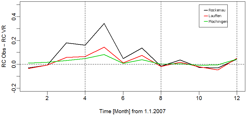
Figure 12 Differences between the runoff coefficient calculated for the three stations for the year 2007 based on observations and simulation.

The results are further evaluated comparing the flow duration curve and the monthly runoff coefficient. The former represents the statistical probability to exceed a specific discharge value within a given time period, while the latter is the ratio between runoff and precipitation over the catchment area. Figure A4 shows the lower exceedance probability compared to the observations, in particular for low discharge rates, a behavior attributed to the lower base flow component and confirmed by the too-low runoff coefficients in spring and summer but similar coefficients during the rest of the year (Fig. 12). We hypothesize that in this period the simulation has a lower hydrological response also due to missing subsurface heterogeneity. As stated above, we have neglected karst features, which are known to produce fast lateral subsurface flows.

Overall, the model captures the general statistical features of the catchment including the typical seasonal trends quite well, while differences are noted related to hydrological extremes and base flow. These differences could be reduced by model calibration from which we refrain because hydrological extremes are not primary the objective of this study. We discuss options to improve the representation of river discharge further below.

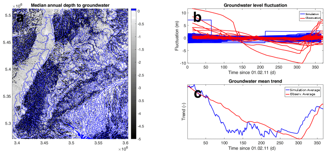
Figure 13 (a) Mean groundwater table depth of the entire domain for the year ranging from 1 February 2011 to 1 February 2012, (b) groundwater fluctuations around a zero mean, and (c) the total mean of all model cells and all real data points superimposed on top of each other to show the annual average trend. Please note that for readability of the figure, panel (a) is limited to a maximum depth of −5 m, while the underlying data ranged down to −88 m.

4.6 Groundwater

A plausibility check of the groundwater levels is performed in two steps. First, we visually inspect the groundwater depth map, shown in Fig. 13a. Accordingly, the model shows a reasonable split between shallower and deeper (5 m and below) groundwater tables compared to expected values from observations with shallower levels overall. Furthermore, the deeper sections are found in the mountainous areas of the model domain, which correspond well with the real situation. It has to be noted though that regions with shallow groundwater levels often show very small values, likely not to be found in the real catchment where the unsaturated zone is usually thicker. In a second step, we compare simulated hydraulic heads with available data. The environmental protection agency of the state of Baden-Württemberg (Landesanstalt für Umwelt, Messungen und Naturschutz – LUBW) operates 33 continuous groundwater observation wells. Comparing those point measurements to simulation results of an uncalibrated model with 400 m grid resolution makes little sense. Instead, we compare (1) the magnitude of the fluctuation in the groundwater table throughout the catchment during a year (calculated as the groundwater observation minus its yearly mean, shown in Fig. 13b), and (2) the average trend of the groundwater level in the full model domain (calculated after subtracting the mean and scaling the fluctuations to have the same magnitude). This means we are comparing standardized anomalies for the observed and simulated groundwater levels. According to Fig. 13b, the magnitude of the groundwater fluctuations is within similar ranges to those of the observations (Fig. 13b), while a few observation wells show larger fluctuations. Also, the fluctuations overall follow similar long-term patterns over the year (Fig. 13c). Hence, the groundwater, given the coarse resolution of the model in comparison with the compared point measurements, shows a reasonable behavior.

5 Discussion

The size of the catchment and resolution considered (400 m) pose an enormous challenge in terms of required CPU time. Still, the applicability of Darcy's law with laboratory-based parameters can be debated as we have to resort to apparent model parameters to produce realistic mass fluxes in the compartments. By compromising these technical and physical aspects in the setup of the virtual Neckar catchment, we experienced several challenges; three of them will be discussed, which we believe to be inherent to simulating energy and mass fluxes across compartment boundaries with partial-differential-equation-based, high-resolution coupled models.

Representation of rivers and surface roughness. River flow in the ParFlow module of TerrSysMP is simulated by an overland flow module. Overland flow appears when hydraulic heads in the top cells are above the land surface. As there is no discrimination between overland flow and river flow, rivers in the simulation have the width of the grid resolution, whereas the real rivers may be significantly narrower. Overland flow is represented in ParFlow with the kinematic wave approximation of the St. Venant equations with the surface friction parameterized by Manning's coefficient. Typical Manning's coefficients when assigned to, e.g., to a 400 m grid cell while in fact the river is much narrower, would result in too-high discharge values during rain events and far-too-low ones during dry periods. In both cases, the always-too-low water levels caused by the too-wide rivers result in a poor representation of river–subsurface exchange. Our current choice of Manning's coefficient in ParFlow ($\mathrm{5.52}\times {\mathrm{10}}^{-\mathrm{4}}$ h m${}^{-\mathrm{1}/\mathrm{3}}$) results in realistic average discharge throughout the year, albeit at too-low flow velocities. In order to compensate for this inconsistency, Manning's coefficient could be scaled such that the overland flow velocity in river cells equals the river flow velocity, as proposed by Schalge et al. (2019), which improves the phasing between simulated and observed discharge and the discharge peak. Similarly, the hydraulic conductivity of the model's top layer for river cells could be scaled in order to reduce the loss of too much surface water to the subsurface caused by the too-wide river cells. These issues will become even more severe when model resolutions are reduced, e.g., for ensemble-based data assimilation because of the even higher demands for computing efficiency.

Coarsening of topography. The still-coarse topography of the simulation reduces the true hill slopes where lateral flow on the surface and in the shallow subsurface takes place. This affects quick-flow components towards rivers. As shown by Shrestha et al. (2015), coarse topography directly impacts the storage of water in the unsaturated zone because drainage becomes less effective. This in turn can lead to an overestimation of latent and underestimation of sensible heat flux. Additionally, coarse-resolution model runs result in delayed and stretched discharge peaks in the rivers. The severity of this effect is proportional to the degree of topography smoothing that is introduced by the coarser resolution; therefore, any change in subsurface parameters such as hydraulic conductivity will depend on the degree of coarsening and the location within a catchment. Especially in narrow valleys and in mountainous areas, this will lead to an overestimation of soil moisture, which we have not yet compensated by changing other parameters. Recently, a method has been proposed to improve these issues by scaling horizontal hydraulic conductivity (Foster and Maxwell, 2019).

Soil parameters. As outlined in Sect. 2, the soil hydraulic parameters were generated based on soil maps of the real Neckar catchment. According to the maps, the soils in the catchment consist mainly of clay and silt, which have rather low saturated hydraulic conductivities and small air entry pressure values. In large areas of the domain, the water content in our first simulations was close to saturation, even for upper soil layers, and the infiltration velocities were unrealistically low. Reasons are the soil parameters, which do not capture the true soil heterogeneity; moreover, real infiltration often takes place in root channels, small fractures, and other small structures. Thus, infiltration is always underpredicted by models using observed soil parameters assuming homogeneity. Infiltration processes may be better captured with dual-domain approaches, which are, however, computationally demanding. A workaround would be to change the soil hydraulic parameters in order to obtain stronger infiltration. Currently, we use an artificially increased sand percentage of the soils in order to stay consistent with the concept of the pedotransfer functions used in CLM. We will also test known scaling rules (e.g., Ghanbarian et al., 2015) to increase, for example, the saturated hydraulic conductivity for larger soil units. These rules should be applied on the soil hydraulic parameters estimated by the pedotransfer functions.

6 Data availability

The presented dataset is available in the CERA database of the German Climate Computing Center (DKRZ: Deutsches Klimarechenzentrum GmbH) (Schalge et al., 2020) at https://doi.org/10.26050/WDCC/Neckar_VCS_v1. The full 9-year time series (2007–2015) for all three compartments has a size of roughly 40 TB in compressed NetCDF4 format. Nevertheless, we encourage the use of this dataset for investigations on data assimilation, but also the general functioning of catchments including cross-environmental interactions and predictability studies can profit from such complete state evolutions of the regional Earth system.

The TerrSysMP model is built in a modular way and users are supposed to get the component models by themselves, while the coupling interface is provided through a git repository (https://github.com/HPSCTerrSys/TSMP, last access: 29 July 2021). As of now, registration is required to access the TerrSysMP git and wiki pages.

Both ParFlow (https://parflow.org/, last access: 29 July 2021) and CLM (http://www.cgd.ucar.edu/tss/clm/distribution/clm3.5/, last access: 29 July 2021) are freely available for download from their respective websites or repositories. COSMO is not available, but the DWD supplies it free of charge for research purposes upon request. More information on this process can be found in the TerrSysMP wiki.

7 Conclusions and outlook

In the present study, we show the development and the data generated based on an integrated subsurface–land-surface–atmosphere system (TerrSysMP, TSMP). Plausibility tests for the derived simulated reality, which tries to mimic the Neckar catchment in southwestern Germany, show that the virtual Neckar catchment is able to reproduce realistic behavior when compared to measurements. Comparisons of simulated precipitation and ABL statistics show a very reasonable agreement with observations. However, comparisons with observed passive microwave measurements by satellites clearly show a systematic bias which is probably related to a mixture of systematic errors in the latter, assumptions in the used forward operator, parameterizations of land-surface properties (soil parameters) in the simulation, and missing processes therein (e.g., preferential flow, hillslope processes). The analysis also shows a realistic connection between evapotranspiration and distance to groundwater in the simulation, while larger deviations from reality are found for river discharge dynamics. The deficiencies could be traced to the model resolution, which limits the often much smaller river widths to multiples of the model resolution, and to the way river discharge is handled in the ParFlow component of TerrSysMP. A new parameterization scheme proposed by Schalge et al. (2019) will avoid such problems in future model simulations. The main issues we face for the upper Neckar are too-high soil moisture and shallow groundwater levels. Several ideas have been proposed to improve the setup including scaling of the surface roughness and soil parameters in response to the results we obtained here. While these changes would show improvements, they are likely marginal or very specific (river discharge characteristics) and would therefore not warrant the great computational cost to rerun for such a long time. Future developments of TerrSysMP may enable this option and it would be interesting to compare resulting datasets and quantify the increase of simulation speed by using GPU compute technologies.

Overall, the results are encouraging regarding the viability of the simulated reality as key input parameters to the land surface and subsurface show very good agreement with observations. For these reasons, the analyses show that the results can be used as a basis for the community for, among others, exploring feedbacks between compartments, identify in which conditions simplification of the models could be done (Baroni et al., 2019) or develop and test methods for assimilating observations across compartments. We encourage the scientific community to explore these data for the different applications. Within the study, we also highlighted some limitations mainly due to the still-severe technical limitation and the IT requirements. We anticipate, however, that more sophisticated versions of simulated catchments (higher resolution, improved parameterization of subscale processes as discussed above) that could be also compared to this dataset in further study are already in progress.

Finally, we want to address the applicability and usefulness of this dataset for various studies. As indicated, this dataset can be valuable for data assimilation both for testing new methods or algorithms and as a standard set for synthetic observations to pull from. It is thus possible to carry out data assimilation experiments with different conditioning datasets. Due to the long time series, we have covered almost any possible weather regime (with the exception of truly extreme events) which can be a great advantage as some algorithms may work well for most conditions but may show weaknesses for other specific conditions (for instance, the CMEM operator in combination with frozen soils). It also allows to investigate the impact of simplifications, such as using a fixed atmospheric forcing instead of a model and thus disregarding feedback mechanisms. Next to data assimilation, there are also model development and model analysis and comparison studies that can benefit from this dataset. If specific changes to the model system are made, for example, testing a new cloud parametrization, all of the input files that are provided with this dataset can be used to quickly set up a working environment with known results to compare to. Here, the length of the simulation is again an advantage since any development can be tested for relevant time slices. A detailed analysis of the dataset regarding compartment interactions is also of interest. We have shown the overall behavior of the system but we have not studied specific interesting events such as heatwaves, dry periods, or floods in detail. It would also be of interest to perform longer-term simulations to analyze climate change and analyze better interannual variability by considering yearly changes in the LAI cycle. Lastly, this setup can also be considered as a template for ensemble-based setups in the future. Right now, reduced resolutions are needed in order to run many members of such a coupled model system. As we have shown, even this higher-resolved simulation still shows some biases that are directly related to resolution, so increasing resolution also in ensembles will be a logical step in the future to obtain better results. When this happens, the methods we used here to generate this simulation will be very useful, along with the analysis presented here to decide how an ensemble should be set up based on the goal (an ensemble for flood forecasts would benefit from a different strategy than an ensemble for drought monitoring).

Appendix A

A1 Appendix tables

Table A1 Values of porosity and hydraulic conductivity of rocks found in Baden-Württemberg.

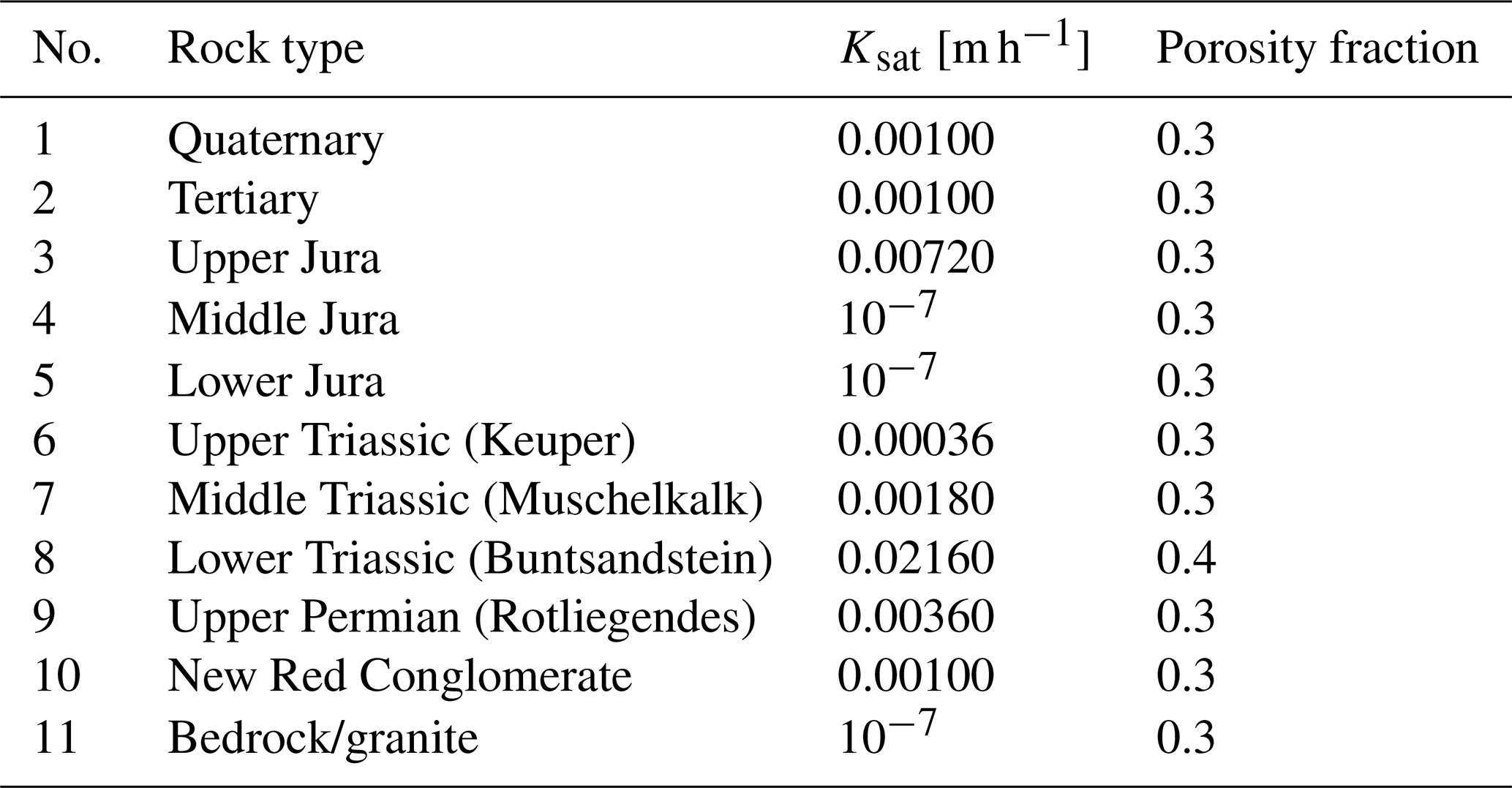
Table A2 Observed atmospheric variables at KIT and STG. Local time at STG is UTC+1.

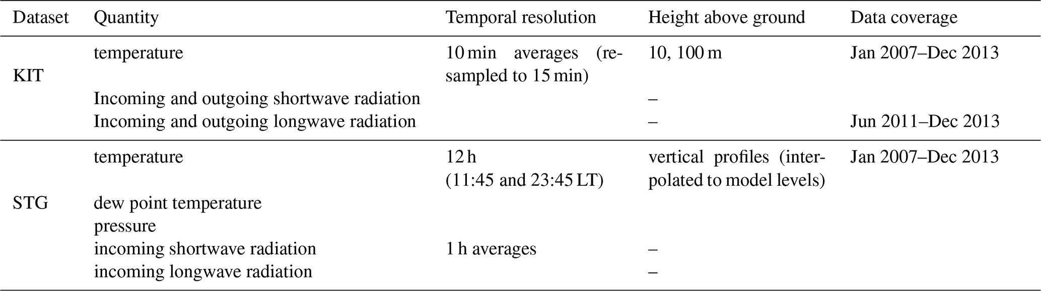
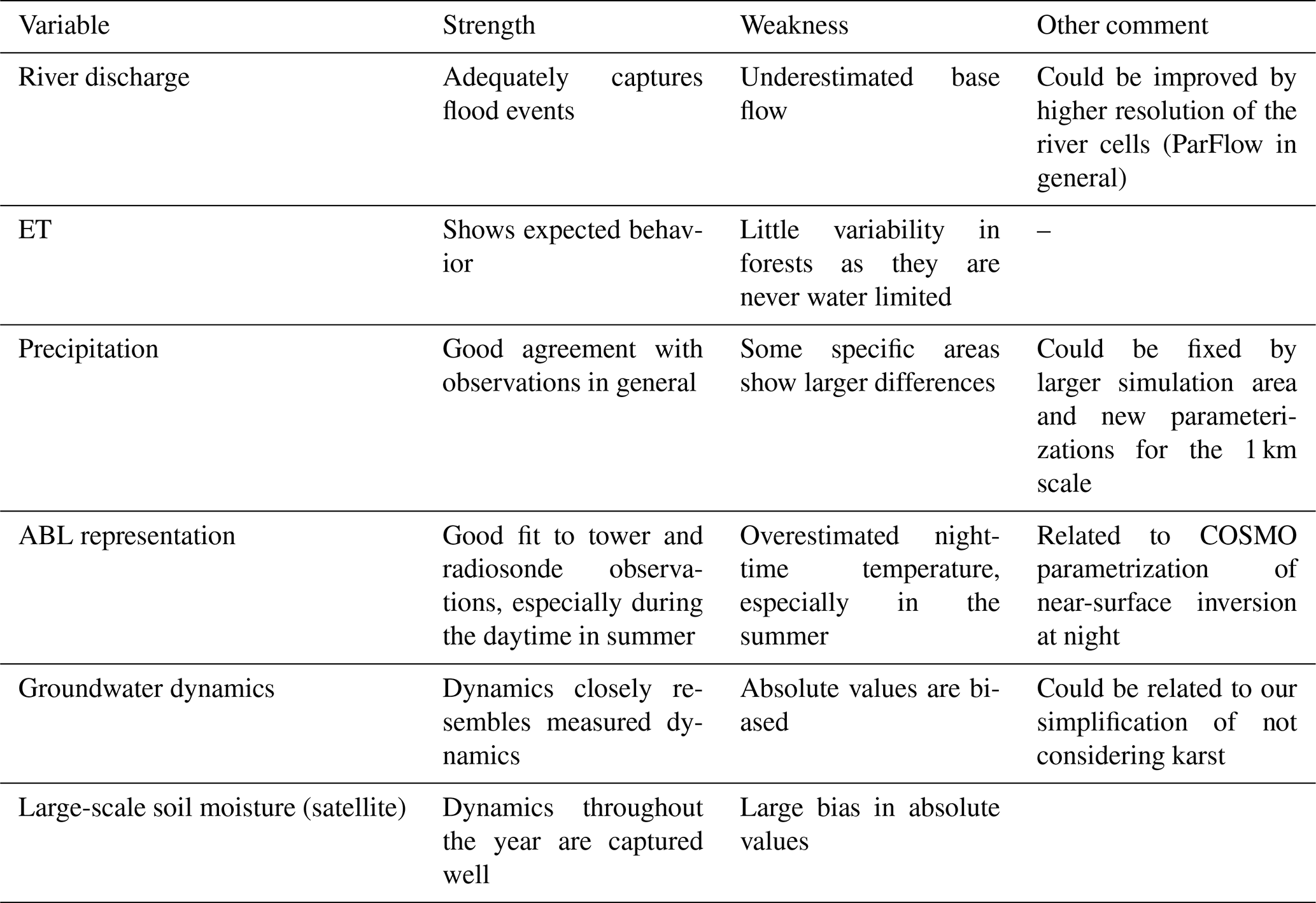
Table A3 Strengths and weaknesses of our simulation regarding several variables.

A2 Appendix figures

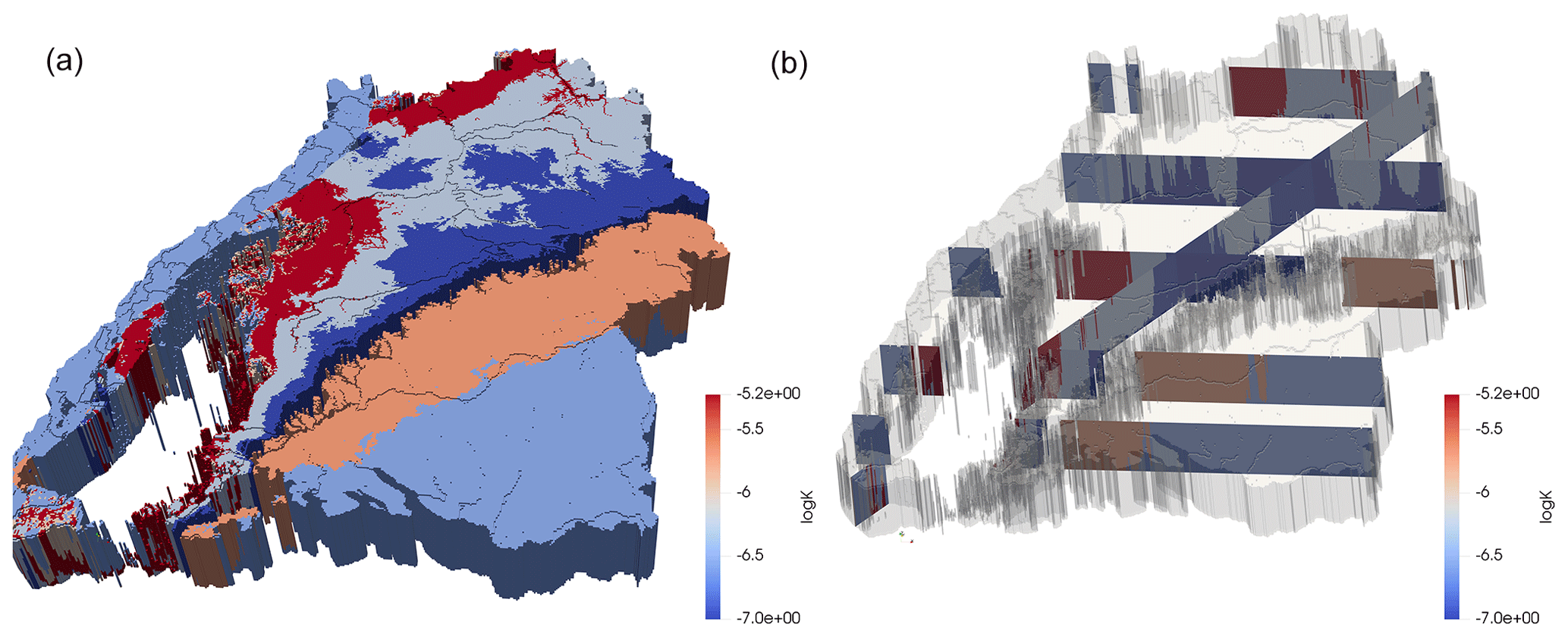
Figure A1 Stratigraphy in the state of Baden-Württemberg represented by its logarithmic conductivity. The left figure shows a 3-D view of the 100 m deep geological model used in this work, where the elevation has been neglected for readability and the transparent region corresponds to low-permeable material. The right figure shows the same using cross-sections to better visualize the vertical heterogeneity.

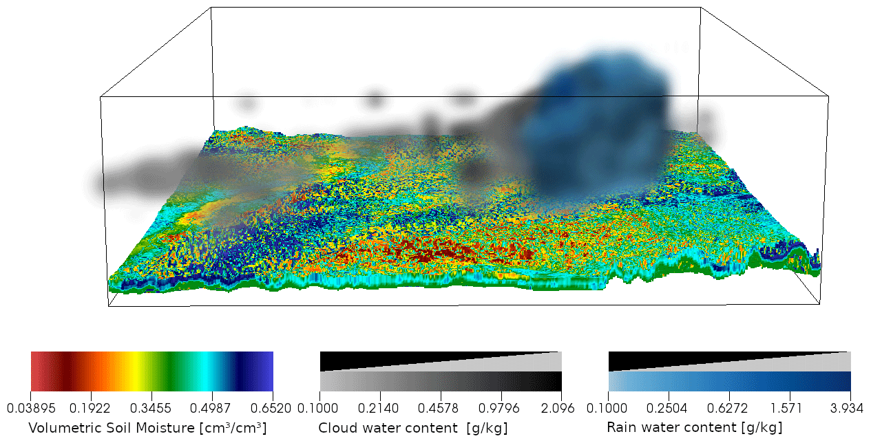
Figure A2 Snapshot of the three dimensional distribution of cloud water/ice (g/kg) (greyscale), precipitation/rainwater (g/kg) (blue in foreground over cloud), and soil moisture (cm³ cm⁻³) (colored) at a time point with a single rain cloud with light rain.

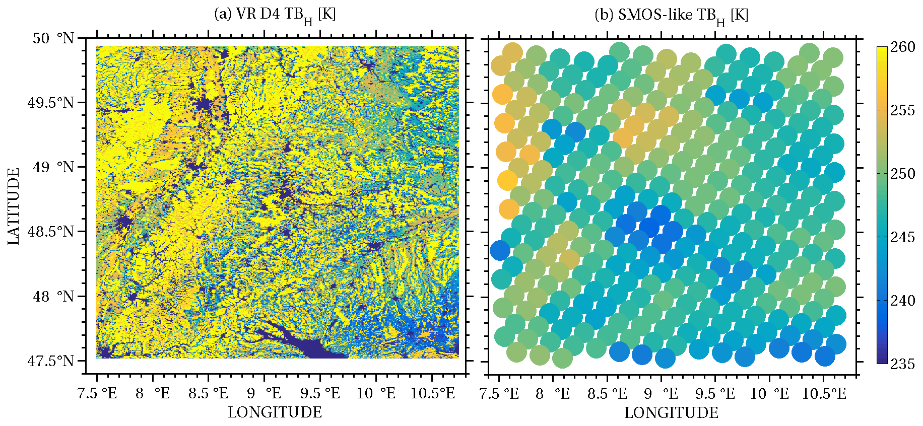
Figure A3 Brightness temperature calculated by the application of CMEM (H polarization) on the simulated-reality output on 2 July 2011 (a) and its aggregation on the spatial resolution of the L1C data product SMOS passive microwave radiometer (b).

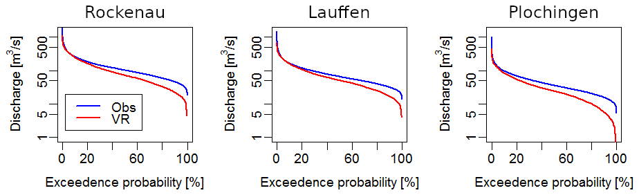
Figure A4 Flow duration curve for the three stations for the 3-year time period is based on. Blue: observations; red: simulated catchment.

A3 Appendix equations

$$\begin{array}{}\text{(A1)}& {\mathit{\sigma }}_{T,t}={\displaystyle \frac{\mathrm{1}}{\text{days}}}\sum \mathrm{|}{T}_{\mathrm{days},t}-{\stackrel{\mathrm{‾}}{T}}_t\mathrm{|}\end{array}$$

Equation (A1): σ is the temperature standard deviation and the subscript t denotes the time of day. This is calculated separately for each month of the year to create the 12 profiles. The overbar for the temperature T denotes the monthly mean temperature value for each time of the day, while the subscript days, t indicates that this is the daily value for the respective time of day.