The 30 m annual land cover dataset and its dynamics in China from 1990 to 2019

Land cover (LC) determines the energy exchange, water and carbon cycle between Earth's spheres. Accurate LC information is a fundamental parameter for the environment and climate studies. Considering that the LC in China has been altered dramatically with the economic development in the past few decades, sequential and fine-scale LC monitoring is in urgent need. However, currently, fine-resolution annual LC dataset produced by the observational images is generally unavailable for China due to the lack of sufficient training samples and computational capabilities. To deal with this issue, we produced the first Landsat-derived annual China land cover dataset (CLCD) on the Google Earth Engine (GEE) platform, which contains 30 m annual LC and its dynamics in China from 1990 to 2019. We first collected the training samples by combining stable samples extracted from China's land-use/cover datasets (CLUDs) and visually interpreted samples from satellite time-series data, Google Earth and Google Maps. Using 335 709 Landsat images on the GEE, several temporal metrics were constructed and fed to the random forest classifier to obtain classification results. We then proposed a post-processing method incorporating spatial–temporal filtering and logical reasoning to further improve the spatial–temporal consistency of CLCD. Finally, the overall accuracy of CLCD reached 79.31 % based on 5463 visually interpreted samples. A further assessment based on 5131 third-party test samples showed that the overall accuracy of CLCD outperforms that of MCD12Q1, ESACCI_LC, FROM_GLC and GlobeLand30. Besides, we intercompared the CLCD with several Landsat-derived thematic products, which exhibited good consistencies with the Global Forest Change, the Global Surface Water, and three impervious surface products. Based on the CLCD, the trends and patterns of China's LC changes during 1985 and 2019 were revealed, such as expansion of impervious surface (+148.71 %) and water (+18.39 %), decrease in cropland (−4.85 %) and grassland (−3.29 %), and increase in forest (+4.34 %). In general, CLCD reflected the rapid urbanization and a series of ecological projects (e.g. Gain for Green) in China and revealed the anthropogenic implications on LC under the condition of climate change, signifying its potential application in the global change research. The CLCD dataset introduced in this article is freely available at https://doi.org/10.5281/zenodo.4417810 (Yang and Huang, 2021).

1 Introduction

Land cover (LC) is an essential component of the Earth system and closely connects the biosphere, atmosphere and hydrosphere. It is usually divided into a range of hierarchical categories, each providing unique habitats and determining the energy exchange, water balances and carbon cycling (Gómez et al., 2016; Houghton et al., 2012; Tang, 2020; Wulder et al., 2018). LC is important for land surface process simulation and is a key variable for environment and ecology models (Schewe et al., 2019; Wulder et al., 2018). In addition, as human settlements sprawled rapidly over the past few decades (Goldewijk, 2001), more demands stressed the terrestrial ecosystem goods and services (Friedl et al., 2010). Consequently, anthropogenic activities have significant implications on LC, water cycling, air quality, food supply and biodiversity (Leng et al., 2015; Li et al., 2020a; Xiao et al., 2018). Accurate and timely LC information is therefore immensely important for climate and environment studies (Herold et al., 2006; Yang et al., 2019), food security (Yang et al., 2020b), sustainable development (Dewan and Yamaguchi, 2009) and resource management (Goetz et al., 2003).

Satellite remote-sensing promotes an efficient LC monitoring by gathering long-term and high-resolution Earth observation (EO) data through orbiting platforms. So far, there have been a lot of studies focusing on LC mapping using satellite data. For example, Sulla-Menashe et al. (2019) used the STEP (System for Terrestrial Ecosystem Parameterization) global training set and long-term Moderate Resolution Imaging Spectroradiometer (MODIS) data to provide annual LC maps that span 2001–2018 (MCD12Q1, 500 m). Besides, the European Space Agency Climate Change Initiative (ESACCI) made an effort to monitor global LC (ESACCI_LC, 300 m) based on multi-source EO data and machine learning (Defourny et al., 2017). More recently, Liu et al. (2020) produced an annual global LC product for 1982–2015 using 5 km GLASS (Global Land Surface Satellite) data. Although these LC products have wide temporal span, their spatial resolution is relatively coarse, which is not sufficient for fine-scale LC monitoring. Furthermore, the uncertainty inherent in LC maps from coarse-resolution data may hinder our understanding on the time-series LC dynamics (Sulla-Menashe et al., 2019).

Recently, the free availability and accessibility of high-resolution EO data (e.g. Landsat) (Woodcock et al., 2008) has enabled fine-scale LC monitoring at a large-scale. In a pioneering effort, Gong et al. (2013) generated the first global 30 m LC map, FROM_GLC (finer resolution observation and monitoring of global land cover), based on Landsat images and 91 433 visually interpreted training samples. More recently, Gong et al. (2019) used training samples derived from the FROM_GLC and multi-temporal Sentinel-2 images to produce a 10 m global LC map for 2017. More recently, Zhang et al. (2020) combined the Global Spatial Temporal Spectra Library and Landsat time series to map 30 global LC types for 2015. However, due to the massive volume of data and the difficulties in obtaining multi-temporal training samples, high-resolution annual or continuous time-series LC products at large-scale have rarely been investigated in the current literature. Specifically, Liu et al. (2014) generated a 30 m LC product (China's land-use/cover datasets, CLUDs) via human–computer interactive interpretation of Landsat images, which documented LC of China from 1980s to 2015 at an interval of 5 years. However, annual LC information is not available for CLUDs due to the tremendous workload and intensive resources involved.

For the past few decades, rapid economic development and population growth has brought about notable implications on LC in China (Yao and Zhang, 2001). Meanwhile, China has implemented a series of ecological projects since the 1980s, such as Gain for Green and Red Lines of Cropland (a policy that China's cropland should be no less than 120 million hectares), which have played an important role in LC changes (Lü et al., 2013; Yin and Yin, 2010). In addition, the climate changes such as frequent precipitation extremes and temperature fluctuations also influenced the LC change of China (Lutz et al., 2014; Zhai et al., 1999). Besides, in the recent decades, rapid urbanization has triggered significant loss of cropland and water. In this context, an annual high-resolution LC product would give us essential insights into both anthropogenic influences and natural changes and help policymakers to implement informed and sustainable management.

In summary, high-resolution annual LC maps for China are still absent. To address this issue, in this research, we produce the annual China land cover dataset (CLCD), which to the best of our knowledge is the first Landsat-derived annual LC product of China from 1990 to 2019. To achieve this, we first automatically derived samples from CLUDs and incorporated them with our visually interpreted samples to obtain multi-temporal training samples. On the other hand, in recent years, the Google Earth Engine has empowered a paradigm shift from traditional per-scene analysis to per-pixel analysis, which enables us to obtain large-scale pixel-wise image composites (Azzari and Lobell, 2017). Therefore, using all available Landsat images (335 709) on the GEE, we calculated a set of spectral, phenological and topographical metrics via pixel-wise temporal composite. Subsequently, we generated CLCD by combining multi-temporal training samples, Landsat-derived temporal metrics and a random forest (RF) classifier. Besides, to enable the LC change monitoring backdate to 1985, we generated a LC map for 1985 as a supplement to the CLCD. Lastly, a spatial–temporal post-processing method involving the spatial–temporal filter and logical reasoning was proposed to ensure the consistency of CLCD. The accuracy of CLCD was validated by two open-source test sets and a visually interpreted test set. In addition, we performed inter-comparison with thematic-class products (i.e. water, forest and impervious surface) to better reflect the quality of CLCD. Based on CLCD, we further analysed the trend of LC changes and conversions in China over the past four decades.

2 Data

2.1 Satellite data

Landsat satellites have been collecting 30 m EO data since the launch of Landsat 5 in 1984, which has been widely recognized as ideal data sources for high-resolution and large-scale LC monitoring. Thus, based on all available Landsat surface reflectance (SR) data on the GEE, we calculated input features including spectrum, phenology and topography. Clouds and cloud shadows in the SR data were identified and removed by the CFmask algorithm (Zhu and Woodcock, 2012). The systematic atmospheric and terrain correction have been conducted for Landsat SR data from all the sensors, i.e. the Thematic Mapper (TM), the Enhanced Thematic Mapper Plus (ETM+) and the Operational Land Imager (OLI), by the United States Geological Survey (USGS). However, given the inconsistent band widths between different Landsat sensors, we used only Landsat 8 OLI data for the CLCD after 2013 and combined TM and ETM+ data before 2013 in view of the good spectral consistency between the two sensors (Micijevic et al., 2016). Due to the uneven spatial coverage of Landsat 5 data in China before 1990 (Pekel et al., 2016), we used all images captured before 1990 to generate the CLCD for the nominal year of 1985 and the CLCD after 1990 was produced annually.

In addition, slope and aspect were computed from the Shuttle Radar Topography Mission (SRTM) data to better reflect topographic changes and detect the LCs growing on steep slopes. Geographic coordinates (i.e. latitude and longitude) were also selected as input data, considering that the distribution of LCs is related to their geographic location.

2.2 China's land-use/cover datasets

China's land-use/cover datasets (CLUDs) documented detailed LC in China for 1980s, 1990, 1995, 2000, 2005, 2010 and 2015. CLUDs were produced by human–computer interaction interpretation of Landsat images, consisting of 6 level-1 classes (cropland, forest, grassland, water, built-up area and barren) and 25 level-2 classes (Liu et al., 2003, 2014). Assessed via field survey, the overall accuracy of CLUDs was reported to be higher than 94.3 % for level-1 classes and more than 91.2 % for level-2 classes (Liu et al., 2014). Although CLUDs were provided at a 5-year interval, its unchanged area can be used as potential training samples. In this study, we therefore proposed to automatically collect training samples via CLUDs data for our 30 m annual LC mapping.

2.3 Third-party validation samples

In addition to the visually interpreted test samples (see Sect. 3.5), we employed two third-party test sample sets to comprehensively validate the quality of CLCD. The first was Geo-Wiki (Fritz et al., 2017), which was a crowdsourced test set covering 10 major LCs (Table S1). Based on the quality flag, we selected 3000 “sure” and “quite sure” Geo-Wiki samples located in China. The other was the Global Land Cover Validation Sample Set (GLCVSS) (Zhao et al., 2014), which followed a random sampling strategy to ensure even distribution of test samples at a global scale. The classification system of the GLCVSS was the same with FROM_GLC (Table S1). We selected 2131 GLCVSS samples covering China to assess the accuracy of CLCD.

2.4 Existing annual LC products

We intercompared the CLCD with the MCD12Q1 and ESACCI_LC to better reflect its quality. The MODIS land cover product (MCD12Q1) in Collection 6 was obtained using a supervised classification method (Sulla-Menashe et al., 2019), which provided global LC from 2001 to 2018 at 500 m resolution. Considering the comparability with the CLCD, the International Geosphere-Biosphere Programme (IGBP) layer in MCD12Q1 was selected and remapped to the CLCD classification system (Table S1). The ESACCI_LC was produced via the GlobCover unsupervised classification chain and multi-source EO data (Bontemps et al., 2013), which documented 300 m global LC during 1992–2018. Likewise, we remapped the class label of ESACCI_LC (Table S1) to facilitate the inter-comparison.

3 Method

This study was aimed at developing the CLCD dataset, and the processing chain included generation of training and test samples, construction of annual input features, classification and spatial–temporal consistency check, and accuracy assessment and product inter-comparison (Fig. 1). The procedure was implemented on the GEE platform, which enabled us to perform pixel-wise analysis and freed us from data download and management (Gorelick et al., 2017). Public data on the GEE, such as Landsat and MODIS, provided long-term Earth observations that helped us composite temporal metrics and collect samples for training and validation. Finally, the accuracy of CLCD was evaluated by the visually interpreted independent samples and the third-party test samples. In particular, we intercompared CLCD with the current state-of-the-art 30 m thematic products including impervious surface area (ISA), surface water and forest to comprehensively assess the quality of CLCD.

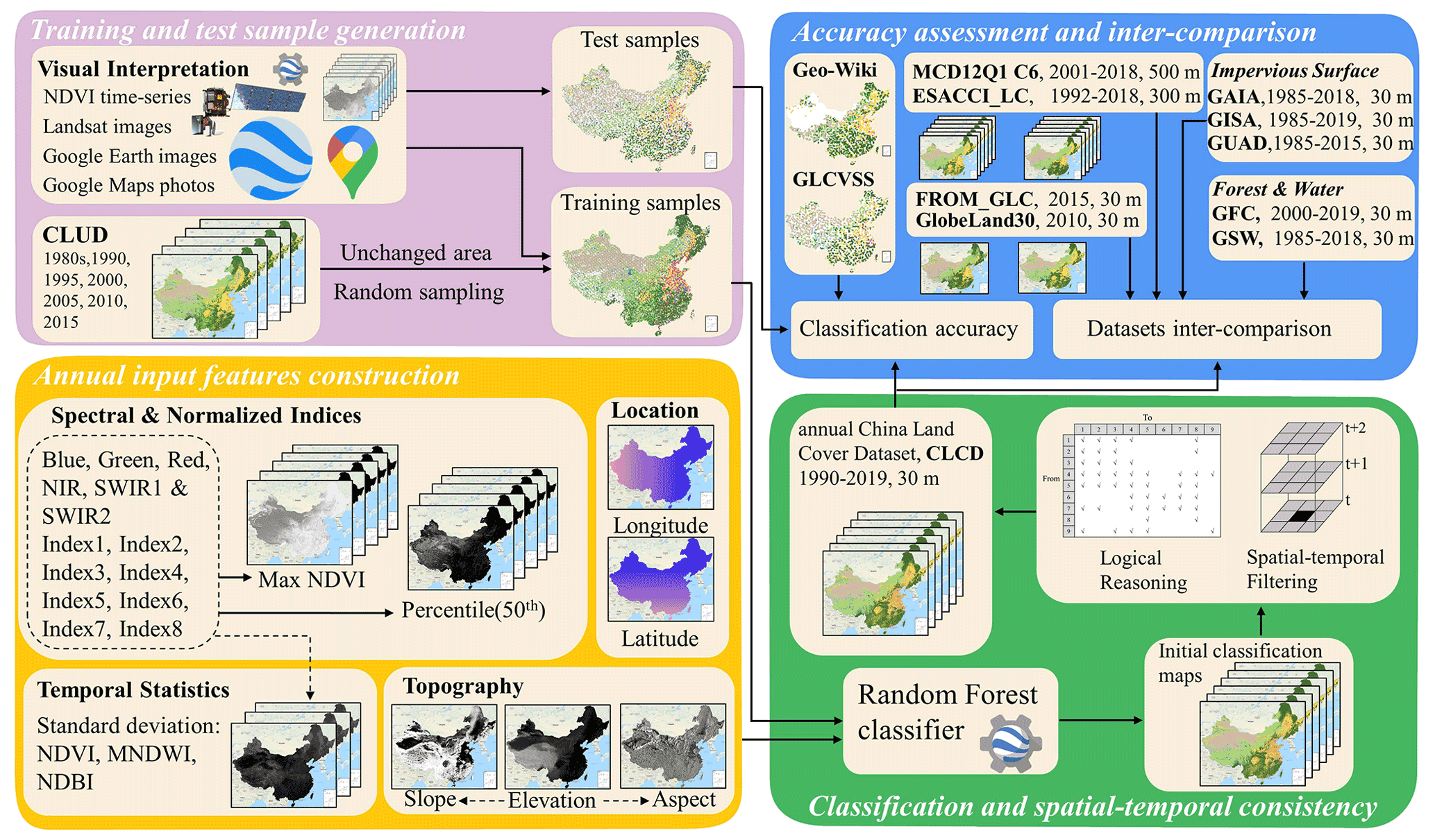
Figure 1 The flow chart to generate the CLCD (annual China land cover dataset).

3.1 Classification system

Considering the LC distribution in China (Liu et al., 2018), we defined a classification system including nine major LCs: cropland, forest, shrub, grassland, water, snow and ice, barren, impervious, and wetland. This classification system is similar to that of FROM_GLC (Gong et al., 2013) and can be conveniently remapped to the FAO (Food and Agriculture Organization) and IGBP systems.

3.2 Input features

The input features to the RF classifier were calculated in terms of spectrum, spectral index, phenology and geographic location (Table 1). Firstly, based on all available Landsat SR within a target year, we calculated the 50th percentile value for each spectral band. Given that spectral indexes can effectively enhance the difference among different LCs (Li et al., 2019), we computed eight spectral indexes to improve the discrimination ability of LC (Table 1). The spectral indexes were mainly constructed by two short-wave infrared (SWIR) bands (e.g. band 5 and 7 for Landsat 5), since SWIR bands have better capability of atmospheric transmission. Besides, as suggested by Li et al., (2020b), to better distinguish between vegetation and non-vegetation, the spectral values of Landsat images corresponding to the maximum NDVI (normalized difference vegetation index) (Tucker, 1979) were included in the spectral features (e.g. Blue_NDVIMax in Table 1), and these spectral values were also used to calculate the aforementioned spectral indexes. Considering the spectral features of different LCs (e.g. vegetation, water) varied throughout the year, we also calculated the standard deviation of these spectral indexes, e.g. NDVI, MNDWI (modified normalized difference water index) (Xu, 2006) and NDBI (normalized difference built-up index) (Zha et al., 2003), to further highlight the phenological information. In summary, 36 features were obtained, including 12 spectral bands, 16 normalized spectral indices, 3 temporal statistics, 3 topographic features and 2 geographical coordinates (Table 1). This approach of using all available images enabled us to (1) reduce the dimension of input features while preserving temporal information and (2) minimize the effects from clouds, shadows or other disturbance.

Table 1 The explanatory table of features used for CLCD mapping^*.

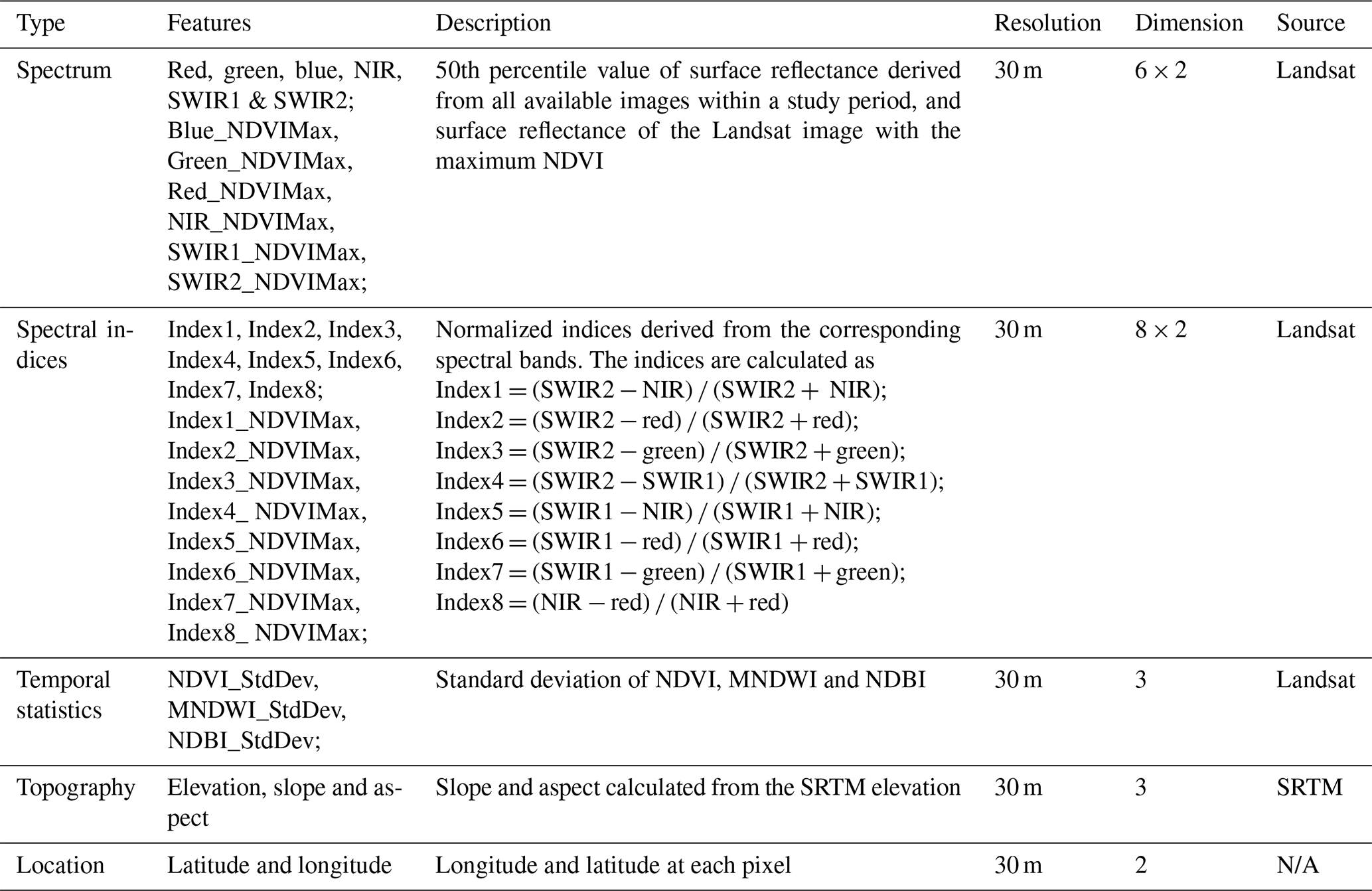
^* Red, green, blue, NIR, SWIR1 and SWIR2 represent the Landsat data in visible band, near-infrared band and short-wave band, respectively. NDVI, MNDWI and NDBI are abbreviations for the normalized difference vegetation index, the modified normalized difference water index and the normalized difference built-up index, respectively.

3.3 Training sample generation

In the case of supervised large-scale LC mapping, accurate and adequate training samples are immensely essential (Foody and Arora, 1997; Foody and Mathur, 2004). Usually, the strategies of training sample collection for a large-scale mapping task include (1) visually interpreted samples and (2) samples automatically derived from existing LC products (Zhang et al., 2021). The visual interpretation method can obtain high-quality samples but require intensive human labour, whereas the automatic sample extraction via existing LC products has the potential for generating a mass of randomly distributed samples, but the sample quality is related to the products used (Jokar Arsanjani et al., 2016; Wessels et al., 2016). Accordingly, the aforementioned two methods were both used to collect training samples in this study. Firstly, given that CLUDs yielded an overall accuracy over 90 % and has been used in a number of studies (Liu et al., 2014), it was considered as a source of training samples. Specifically, we selected the regions with stable LC throughout all periods of CLUDs (i.e. 1980s, 1990, 1995, 2000, 2005, 2010, 2015) to further ensure the reliability of samples. In such a way, we obtained a candidate sample pool of China. Then, the study area was divided into 1665 hexagons with 0.5^∘ sides (Fig. 2a), and 20 points were randomly generated within each grid to ensure their spatial distribution and diversity. Finally, a total of 27 000 training samples were randomly selected.

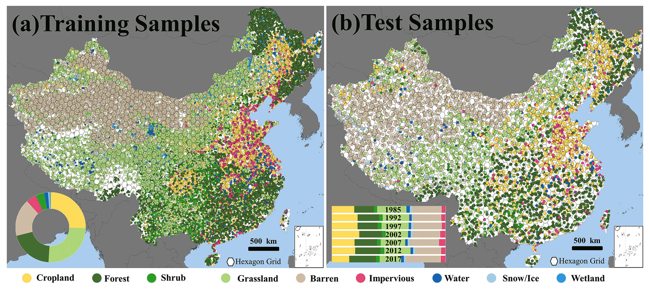
Figure 2 Spatial distribution of visually interpreted training and test samples. The proportions of each land cover class were shown in the inner graphs.

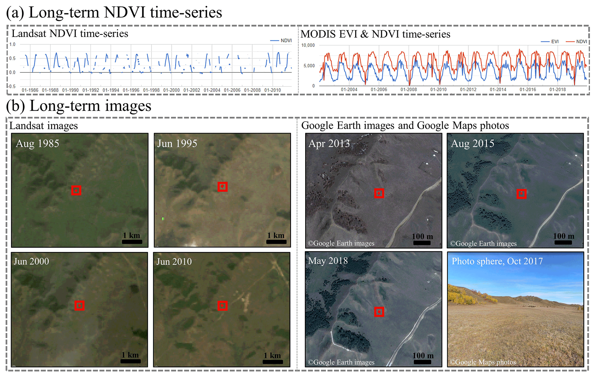
Figure 3 An example of auxiliary data used to interpret the training samples, including Landsat NDVI time series, MODIS NDVI and EVI time series, Landsat images, Google Earth images, and Google Maps photos. The red dot represents a sample site located at 42.541067^∘ N, 117.146569^∘ E.

Gong et al. (2019) has demonstrated that it is possible to use training samples of circa 2015 to classify the LC map of 2017. However, given that CLUDs were not available after 2015, we manually interpreted 2200 unchanged sites over the entire study period (i.e. 1985–2019) to further ensure the accuracy of the long time-series products. For manual interpretation, we referred to Google Earth high-resolution images, MODIS EVI (enhanced vegetation index) and NDVI time series, and Landsat images and their NDVI time series. Specifically, we first checked the Landsat NDVI time series (1985–2019) and the MODIS EVI/NDVI time series (2001–2019) for a candidate sample site. If its NDVI time-series curves were stable (Fig. 3a), the site was regarded as unchanged, and its LC label was then determined via Google Earth images and Landsat images. In particular, for the sites where Google Maps photos or photo spheres were available, these photos were also used to interpret the LC labels. Taking the red dot in Fig. 3 for instance, its NDVI time-series features were stable (Fig. 3a), signifying that it was unchanged and was hence regarded as a potential sample site. It is difficult to determine whether it is bare soil or withered grassland even in high-resolution Google Earth images, owing to the sample point's relatively smooth texture. In this case, by courtesy of the Google Maps photo sphere, we were able to interpret the actual LC label (i.e. grassland) (Fig. 3b). In total, we selected and interpreted 2200 sites, accounting for 18 000 Landsat pixels. Combined with the aforementioned automatically generated training samples from the CLUDs, we finally collected 45 000 training samples in total (Fig. 2a), which were used in the annual classifications.

3.4 Classification and spatial–temporal consistency

The random forest (RF) classifier is commonly used for large-scale LC mapping (e.g. Belgiu and Drăgu, 2016; Zhang and Roy, 2017; Zhang et al., 2020) due to a number of advantages, such as the ability to handle high-dimensional data, the tolerance to sample errors and the robustness to missing data (Bauer and Kohavi, 1999; Wulder et al., 2018). Therefore, RF classifier was used to generate the CLCD. The number of trees was set to 200 (Liu et al., 2020a). Based on the training samples, classifiers were trained by input features constructed via Landsat SR from the target year as well as two adjacent years, and the preliminary classification results were obtained by the trained RF classifiers.

To further ensure the accuracy and reliability of the classification results, we proposed a spatial–temporal post-processing method, consisting of a spatial–temporal filter and logical reasoning, to refine the time-series mapping results. This method leveraged spatial–temporal context as well as the prior knowledge to suppress the illogical LC conversions. Such errors were usually induced by misclassifications (Wehmann and Liu, 2015). Firstly, the spatial–temporal filter was carried out within a $\mathrm{3}\times \mathrm{3}\times \mathrm{3}$ spatial–temporal window (Li et al., 2015). Specifically, for pixel i with a LC label L_i,t in year t, if the label of i in pervious year (i.e. $L_{i,t-\mathrm{1}}$) was not equal to L_i,t, a LC conversion may take place. In this situation, we further checked the spatial–temporal consistency probability P_i,t of pixel i using the following equation:

$$\begin{array}{}\text{(1)}& P_{i,t}={\displaystyle \frac{\mathrm{1}}{N}}\left[{\sum }_t^{t+\mathrm{2}}{\sum }_{x-\mathrm{1}}^{x+\mathrm{1}}{\sum }_{y-\mathrm{1}}^{y+\mathrm{1}}I(L_{i,t}=L_j)\right],\end{array}$$

where L_j denotes the LC label for pixels in the current window and N represents the total number of pixels (i.e. N=27). I ($L_{i,t}=L_j$) is the indicator function, i.e. I=1 if L_i,t equals to L_j and I=0 otherwise. Besides, x and y indicate the location of i. A higher P_i,t value signifies the LC conversion, but a lower P_i,t value may correspond to a classification error. Here we set a simple rule to check whether the LC change takes place: if the value of P_i,t is greater than 0.5, the label of the pixel in year t is considered changed. A value of P_i,t less than 0.5 corresponds to an incorrect classification, and hence the label of this pixel is actually not changed. In such a case, L_i,t should be corrected as $L_{i,t-\mathrm{1}}$. In addition, the CLCD followed the assumption that a LC change should last for more than 2 years (Defourny et al., 2017).

On the other hand, we defined a logical reasoning method via a transition matrix (Table S2) to suppress illogical LC conversions. For example, it is not likely for a pixel to change from barren to cropland within a year. The matrix was inspired by He et al. (2017), but was modified according to the LC changes in China over the past four decades. For instance, China has built many reservoirs in the past 30 years (Li et al., 2018), leading to a mass of cropland covered by water. Thus, conversion from cropland to water should be considered.

3.5 Accuracy assessment

In order to assess the accuracy of CLCD, three independent test sets covering the whole China were used: (1) two third-party test sets (i.e. Geo-Wiki and GLCVSS) and (2) a visually interpreted test set (5463 in total) for seven years (i.e. 2017, 2012, 2007, 2002, 1997, 1992, 1985), with each year containing around 750 samples. To ensure their random distribution, the visually interpreted points were sampled following the same sampling strategy as the training sample selection (Fig. 2b). Likewise, the Google Earth images, Landsat images and MODIS EVI time series were used for the interpretation. The spatial distribution of the visually interpreted test samples was shown in Fig. 2, where the bars represented the proportions of each LC for different years. Finally, the accuracy of CLCD was assessed by confusion matrixes, including producer's accuracy (PA), user's accuracy (UA), overall accuracy (OA) and F1 score. The F1 score conveys the balance between PA and UA and is calculated as

$$\begin{array}{}\text{(2)}& \text{F1}=\mathrm{2}{\displaystyle \frac{\text{PA}\times \text{UA}}{(\text{PA}+\text{UA})}}\times \mathrm{100}\mathit{\%}.\end{array}$$

3.6 Datasets inter-comparison

In addition to the existing annual LC products (i.e. MCD12Q1 and ESACCI_LC), the CLCD was also compared with several Landsat-derived thematic datasets for more comprehensive quality evaluation. Specifically, with respect to some dynamic LCs (i.e. impervious surfaces, forests and surface water), we intercompared the CLCD with the Global Forest Change (GFC) (Hansen et al., 2013), Global Impervious Surface Area (GISA) (Xin et al., 2021), Global Artificial Impervious Area (GAIA) (Gong et al., 2020), Global Annual Urban Dynamics (GAUD) (Liu et al., 2020b) and the Global Surface Water (GSW) (Pekel et al., 2016) datasets. For the GSW dataset, over 3 million Landsat images were used to map global surface water from 1985 to 2015, with PA more than 95 % and UA over 99 % (Pekel et al., 2016). The GFC data depicted global forest changes from 2000 to 2013 using 30 m Landsat data (Hansen et al., 2013). The GISA, GAIA and GAUD were Landsat-derived annual ISA (or urban) products for periods 1972–2019, 1985–2018 and 1985–2015, respectively. Specifically, as suggested by Zhang et al., (2020), the aforementioned thematic products were aggregated within the spatial grid of $\mathrm{0.05}{}^{\circ }\times \mathrm{0.05}{}^{\circ }$ to obtain the area fraction and the scatterplot and linear regression with the correlation coefficient (R²) and root mean square error (RMSE) quantitative metrics, which were used to demonstrate their agreement.

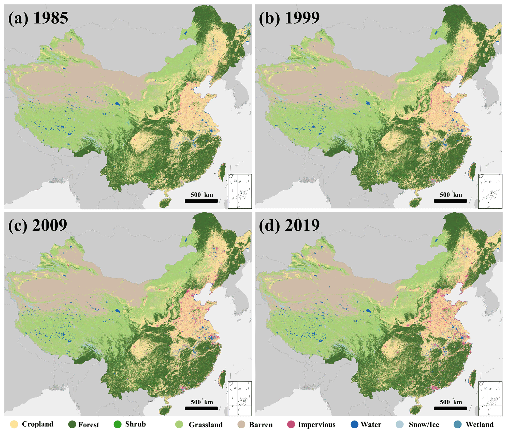
Figure 4 Annual China land cover dataset (CLCD) for 1985, 1999, 2009 and 2019.

4 Results and discussion

4.1 Accuracy assessment of CLCD

Based on all available Landsat SR data on the GEE, we generated the annual China land cover dataset (CLCD). The accuracy of CLCD was first assessed via visually interpreted independent samples (Tables S3–S9). Overall, the accuracy of CLCD was stable and satisfactory (76.45 % < OA < 82.51 %), with average OA of 79.30 % ± 1.99 % (Fig. 5i). For each category, water achieved the highest average F1 score (87.06 % ± 7.07 %), followed by the forest (85.49 % ± 1.30 %), snow/ice (83.51 % ± 7.99 %) and barren (81.85 % ± 4.15 %) classes. The accuracy was relatively high for grassland and impervious area, with a mean F1 score over 72 %. In addition, CLCD outperformed MCD12Q1 and ESACCI_LC in terms of OA in all the years (Tables S10–S19). For the LCs with a relatively large proportion in area, such as cropland, forest and grassland, CLCD also exhibited better and more stable F1 scores with respect to the MCD12Q1 and ESACCI_LC (Fig. 5).

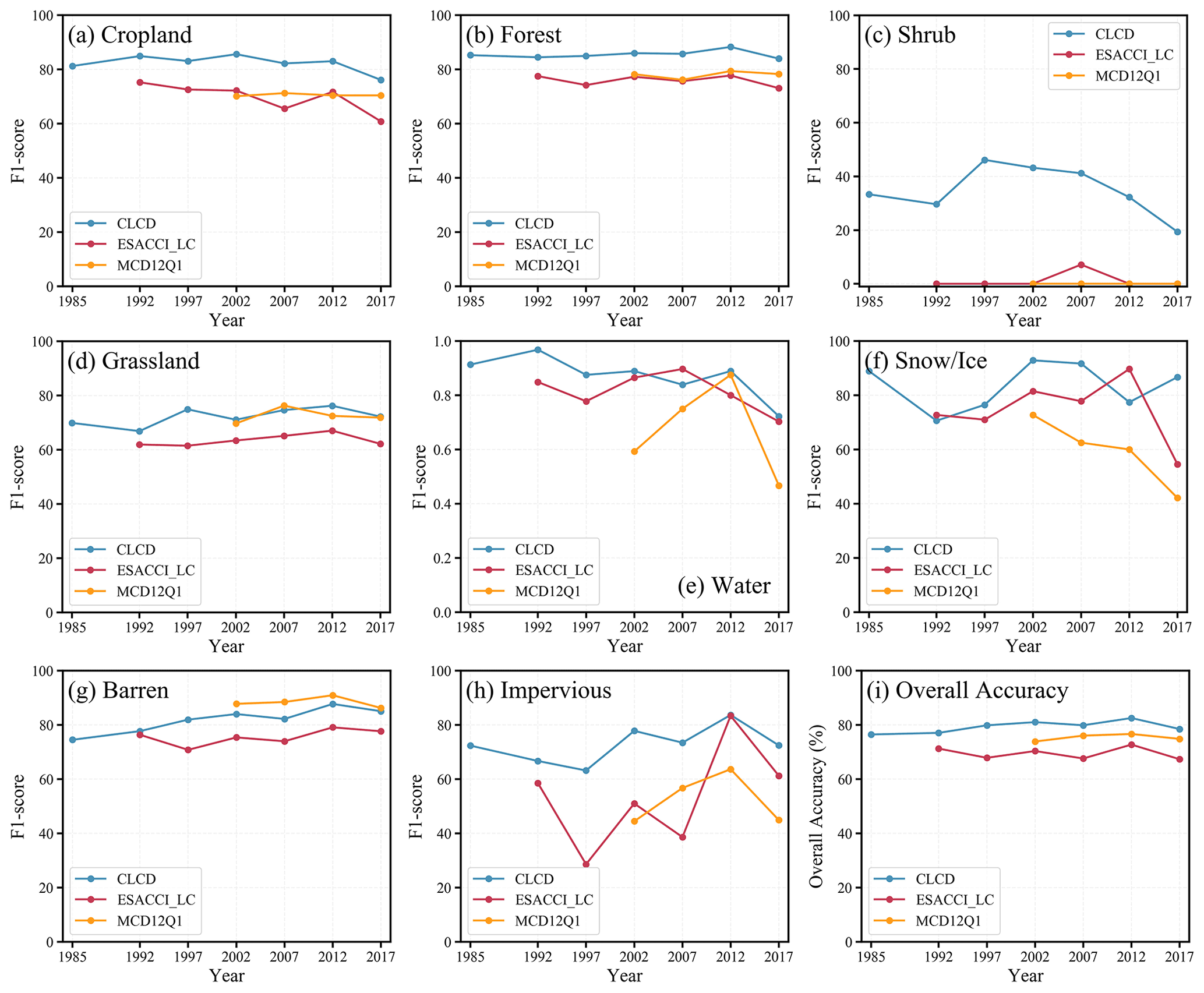
Figure 5 F1 score and overall accuracy for ESACCI_LC, MCD12Q1 and CLCD based on visually interpreted test samples.

Table 2 Comparison of mapping accuracy based on Geo-Wiki test samples for ESACCI_LC, MCD12Q1, FROM_GLC and CLCD^*.

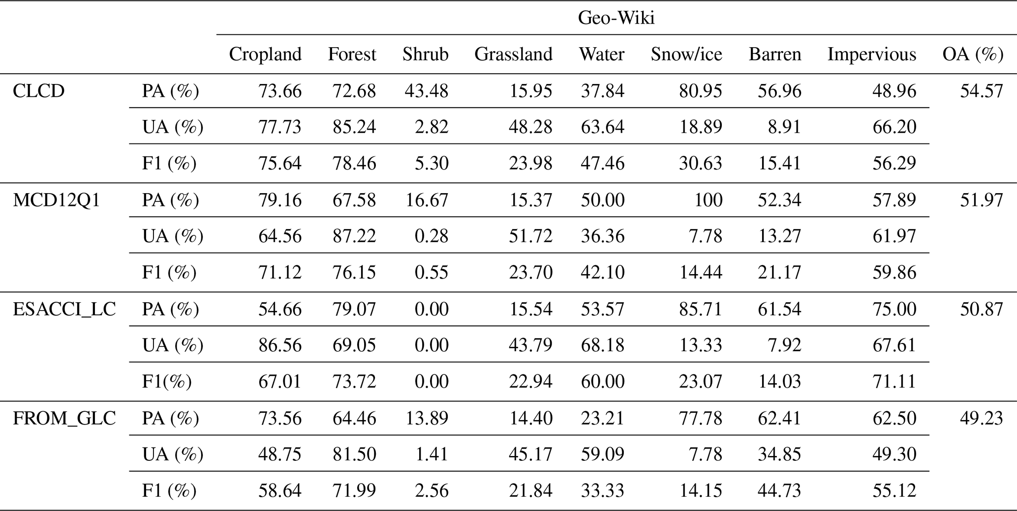
^* PA, UA and OA are abbreviations for the producer's accuracy, user's accuracy and overall accuracy respectively. The F1 represents the harmonic mean of the PA and the UA.

To better validate the accuracy of CLCD, we used the Geo-Wiki samples to intercompare the CLCD, FROM_GLC, MCD12Q1 and ESACCI_LC. The first global 30 m LC data were from FROM_GLC (Gong et al., 2013). Here we adopted its second-generation product, which was generated using Landsat images acquired from 2013 to 2015 (Li et al., 2017). Overall, the CLCD possessed a better OA of 54.57 % against the ESACCI_LC (50.87 %), the MCD12Q1 (51.97 %) and the FROM_GLC (49.23 %), respectively (Tables S20–S23). Specifically, CLCD achieved better accuracy than FROM_GLC in most LCs and showed similar performance for the impervious area (Table 2).

We also compared the accuracy of different products (i.e. CLCD, GlobeLand30, MCD12Q1 and ESACCI_LC) using the GLCVSS sample set. In particular, GlobeLand30 was also included for comparison to our CLCD. GlobeLand30 was a 30 m global LC dataset for 2001 and 2010, produced using a pixel–object-knowledge approach (Chen et al., 2015). We used GlobeLand30 in the year of 2010 for the comparison. It was found that the CLCD obtained the highest accuracy of 65.64 %, outperforming ESACCI_LC (57.16 %), the MCD12Q1 (61.66 %) and GlobeLand30 (63.12 %), respectively (Tables S24–S27). Although the UA or PA of CLCD did not always outperform that of other products, CLCD achieved the highest F1 scores in nearly all the LCs (Table 3).

We calculated the confusion matrix for CLCD without spatial–temporal filtering. It was indicated that the overall accuracy of CLCD without the spatial–temporal filtering was dropped by 0.71 compared to that with spatial–temporal filtering (Tables S28 and S29). This showed the effectiveness of our proposed post-processing method.

In summary, CLCD achieved higher OA with respect to the existing LC products (i.e. MCD12Q1, ESACCI_LC, FROM_GLC and GlobeLand30), based on the visually interpreted and third-party samples. In addition, the temporal coverage of CLCD spans 35 years (1985–2019), which exceeds the ESACCI_LC (1992–2018) and the MCD12Q1 (2001–2018).

Table 3 Comparison of mapping accuracy based on GLCVSS (Global Land Cover Validation Sample Set) test samples for ESACCI_LC, MCD12Q1, GlobeLand30 and CLCD^*.

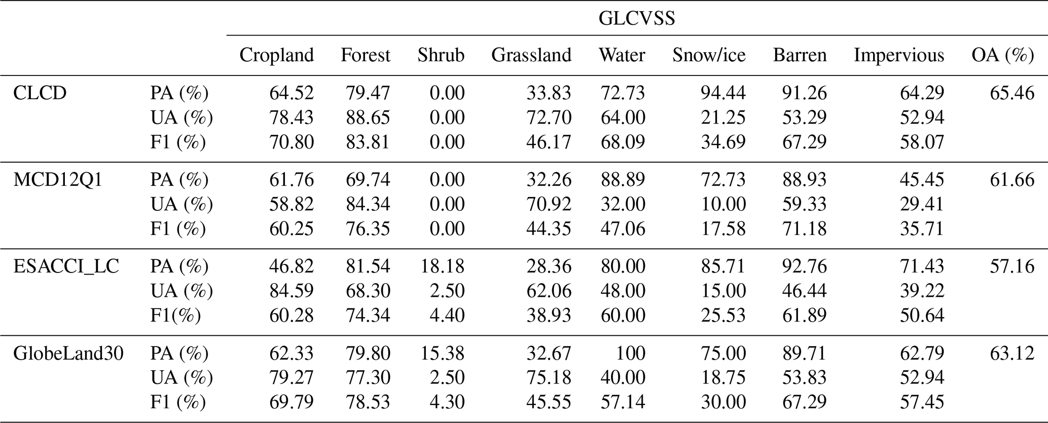
^* PA, UA and OA are abbreviations for the producer's accuracy, user's accuracy and overall accuracy respectively. The F1 represents the harmonic mean of the PA and UA.

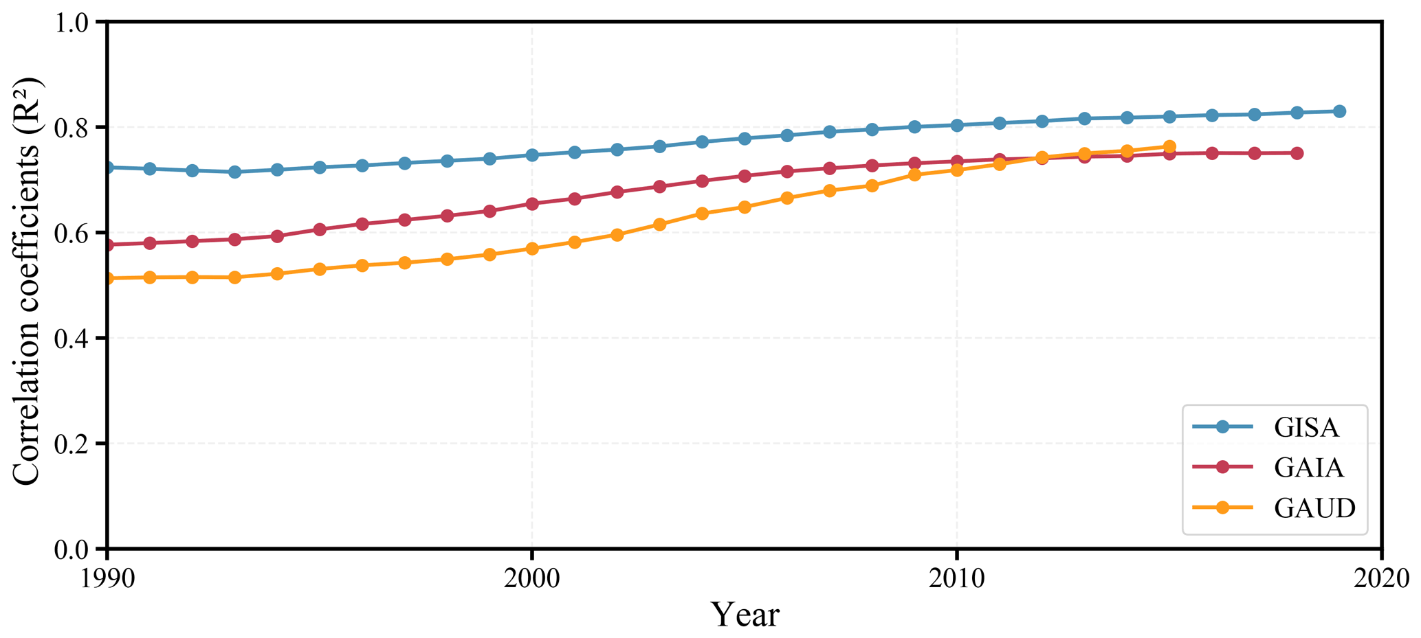
Figure 6 The correlation coefficients of the ISA fraction between CLCD and three thematic datasets for each year. ISA fraction was aggregated within the 0.05^∘ by 0.05^∘ spatial grid.

4.2 Inter-comparison with existing 30 m thematic products

4.2.1 Comparison with ISA

The impervious surface area (ISA), as the consequence of urbanization, has rapidly sprawled in the past few decades and had significant implications on regional ecological changes (Goldewijk, 2001). In view of the fast urbanization in China, the accuracy of CLCD can be validated by the accuracy of ISA. Thereby, we compared the ISA of CLCD (CLCD-ISA) with the existing well-known 30 m annual ISA products (i.e. GISA, GAUD, GAIA). We first calculated ISA fractions within the $\mathrm{0.05}{}^{\circ }\times \mathrm{0.05}{}^{\circ }$ spatial grid for each year and estimated the correlation coefficients between CLCD-ISA and the three thematic datasets to quantitatively demonstrate their agreement. Overall, the CLCD-ISA showed good consistency with the existing ISA products ($\mathrm{0.51}<R^{\mathrm{2}}<\mathrm{0.83}$), indicating the reliability of our CLCD products (Fig. 6). Although good agreement has been found between CLCD-ISA and other products in most years, the correlation between CLCD-ISA and GAUD in 1995 was only 0.53. This was probably subject to the underestimations of villages in GAUD during early years since GAUD focused on the urban areas. It can be seen in Fig. 7 that CLCD-ISA and GISA were generally similar, while GAIA and GAUD had a little omission over the North China Plain where villages gather.

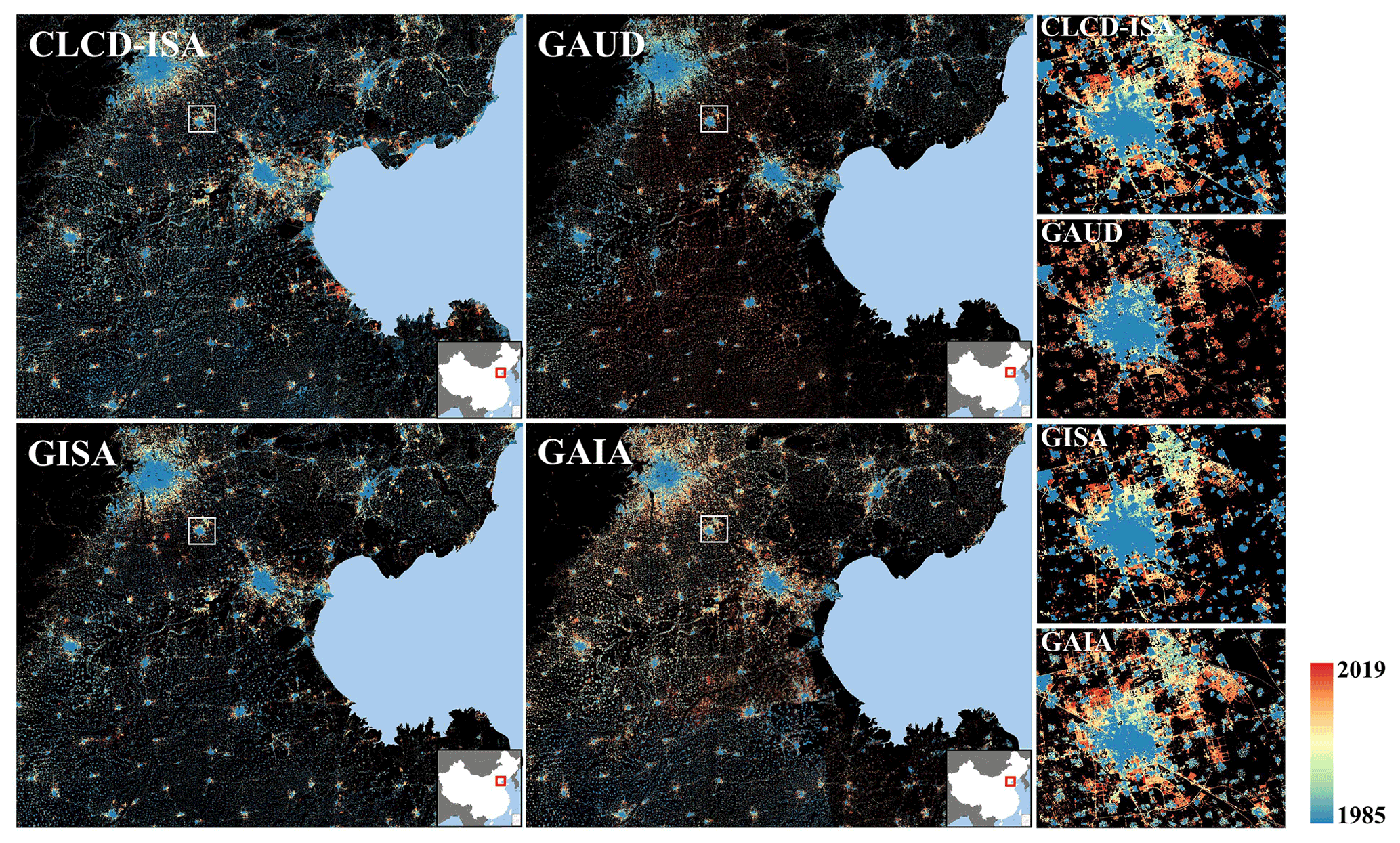
Figure 7 Comparison between different ISA products over the North China Plain, with close-up maps located in Langfang city (39.526545^∘ N, 116.703692^∘ E).

4.2.2 Comparison with forest change

We further compared the forest in CLCD (CLCD-forest) with the Global Forest Change (GFC) data from Hansen et al. (2013) to demonstrate the accuracy of CLCD. The GFC data (v1.7) included forest cover as fraction (2000), forest gain (2001–2019 as total) and year of forest loss. Since the year of forest gain was unavailable, we selected the areas with forest cover greater than 30 % as forest to obtain the 2000 and 2019 forest map, as suggested by Taubert et al. (2018). Based on the above forest maps, the forest fraction was aggregated within the $\mathrm{0.05}{}^{\circ }\times \mathrm{0.05}{}^{\circ }$ spatial grid. It was found that CLCD-forest showed relatively high agreement with the GFC ($\mathrm{0.84}<R^{\mathrm{2}}<\mathrm{0.87}$), signifying the reliability of CLCD. Additionally, as can be seen in the Fig. 9, the spatial distribution of CLCD-forest was generally similar to the GFC data.

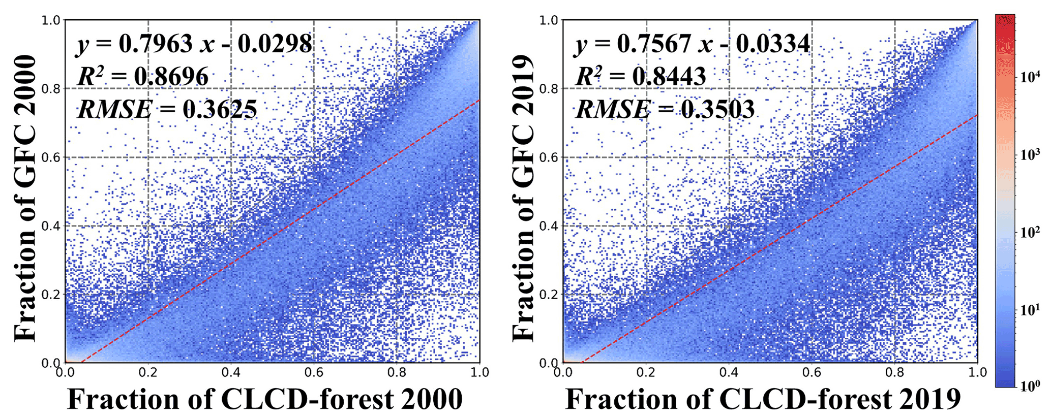
Figure 8 Scatterplots of forest fraction between the CLCD and GFC in 2000 and 2019. Forest fraction was aggregated within the 0.05^∘ by 0.05^∘ spatial grid.

Figure 9 Example of 2019 forest maps for CLCD and GFC located at the Lesser Khingan Mountains (47.703792^∘ N, 129.388820^∘ E).

4.2.3 Comparison with surface water

Surface water in China has changed dramatically over the past decades due to comprehensive implications of human activities and climate changes (Lutz et al., 2014; Yang et al., 2020a). Therefore we assessed the quality of the CLCD dataset through inter-comparison of the Global Surface Water (GSW) (Pekel et al., 2016). The GSW (v1.2) data were the first 30 m dataset that documented the monthly persistence and existence of surface water from 1985 to 2018. It should be noted that CLCD used the annual median reflectance (i.e. 50th percentile), and hence its water extent (CLCD-water) was close to the average annual water extent. The GSW, on the other hand, had a denser temporal sequence (monthly). Accordingly, to facilitate the inter-comparison, we obtained GSW average annual water extent based on the intra-annual water occurrence (Yang et al., 2020a). In this manner, we selected GSW and CLCD-water in 1995, 2005 and 2015, and we calculated the water fraction of the two datasets within the $\mathrm{0.05}{}^{\circ }\times \mathrm{0.05}{}^{\circ }$ spatial grid. As demonstrated in Fig. 10, the high consistency ($\mathrm{0.86}<R^{\mathrm{2}}<\mathrm{0.96}$) was achieved with two products, indicating the reliability of CLCD.

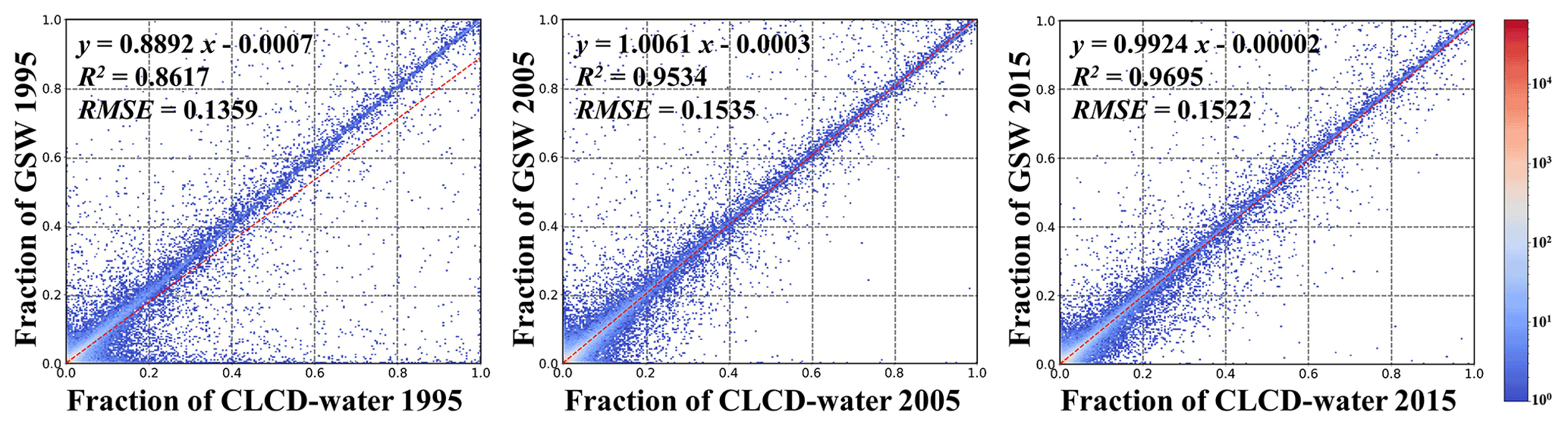
Figure 10 Scatterplots of surface water fraction between CLCD and GSW in 1995, 2005 and 2015, respectively. Water fraction was aggregated within the 0.05^∘ by 0.05^∘ spatial grid.

To better explain the difference of two products in depicting water dynamics, we counted the number of water occurrences from 1985 to 2018. A higher occurrence signifies permanent water, while a lower occurrence indicates seasonal or new permanent water. As shown in Fig. 11, the CLCD-water extent was closely similar to the GSW water extent, which again demonstrated the reliability of CLCD. However, we noted that GSW captured more seasonal water (Fig. 11b and d). This was expected, as GSW had a denser temporal sequence (monthly) than CLCD (annual). Consequently, it is difficult for CLCD to capture short-term fluctuations (e.g. flooding). However, long-term changes caused by anthropogenic activities, such as reservoir construction, were accurately observed by CLCD (Fig. 11a and c).

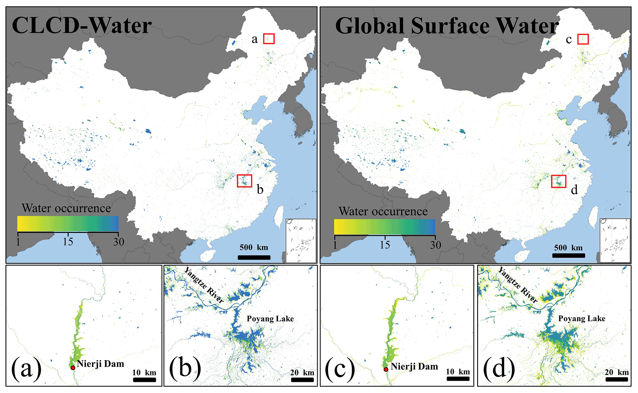
Figure 11 Annual water occurrence (1985–2018) derived from water extent of CLCD and GSW, with close-up maps located in Nierji Dam (a, c) and Poyang Lake (b, d).

4.3 LC dynamics in China 1985–2019

4.3.1 General temporal trend

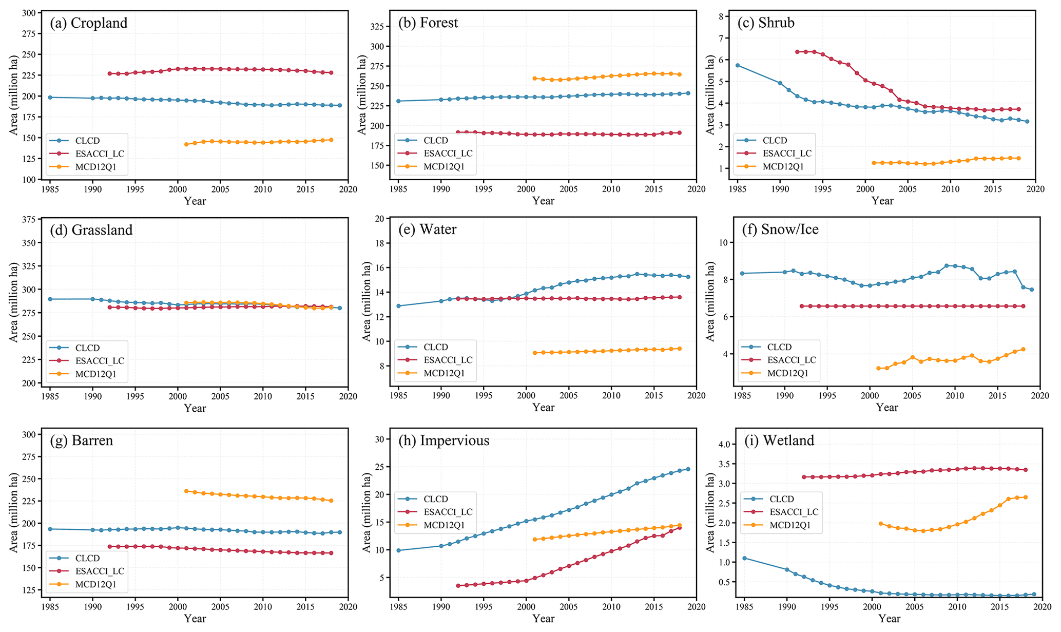
Based on the CLCD generated in this study, we analysed the LC changes in China from 1985–2019 (Fig. 12). The impervious area has unprecedentedly sprawled over the past 35 years, with more than 24.5 million ha in 2019, which was increased by 1.5 times relatively to that in 1985. In terms of change in magnitude, the impervious area also exceeded the rest, with 46.56 % more than the second-ranked forest. The area of surface water increased by 2.37 million ha, 78.40 % of which occurred after 1995 when the development of hydropower was proposed by the Ninth Five-Year Plan of China (Li et al., 2018). The increasing reservoirs resulting from dam construction are one of the reasons that accounted for the surface water extension (Yang et al., 2020a). Although northeast and northwest China have undergone extensive reclamation to feed the growing population, cropland has generally decreased. In particular, 4.57 % of cropland was lost during 1985–2010, but it should be emphasized that only 0.03 % was lost after the implementation of Red Lines of Cropland in 2010 (Xie et al., 2018). Due to a series of afforestation policies in China, such as the Three-North Shelterbelt project started in the 1980s and the Gain for Green project initialized after 2000, the forest had increased by 4.34 % (10.02 million ha) from 1985 to 2019 (Fig. 12b). The shrub decreased by 2.59 million ha, with similar decrease trends found with ESACCI_LC (Fig. 12c and Liu et al., 2020a). The barren class increased slightly by 0.80 % from 1985 to 2000 but decreased by 2.62 % from 2000 to 2019. The decrease in the barren class may be related to the ecological project Returning Grazing Land to Grassland after 2003 (Xiong et al., 2016). In contrast, grassland decreased by 2.15 % (6.23 million ha) before 2000 but only 1.16 % (3.28 million ha) from 2000 to 2019 thanks to the implementation of grassland conservation policies such as the Gain for Green after 2000 (Li et al., 2017). The wetland decreased by 0.92 million ha, 91.3 % of which occurred before 2000, which was likely attributed to the extensive reclamation that occurred in the Sanjiang Plain of northeast China before 2000 (Zhang et al., 2010, 2009).

Compared with ESACCI_LC and MCD12Q1, CLCD showed generally similar trends. However, it should be noticed that the CLCD detected more surface water and impervious area with respect to two coarse-resolution LC products (Fig. 12). This was attributed to the discernible resolution (30 m) of Landsat data, which allow better delineation of relatively small LC patches. Therefore, the 30 m CLCD data are more applicable in the fine-scale environment and land surface process simulation.

Figure 12 Temporal changes in area of different land covers in China from 1985 to 2019.

Table 4 Ratio (%) of land cover conversions from 1985 to 2019.

4.3.2 LC conversion patterns

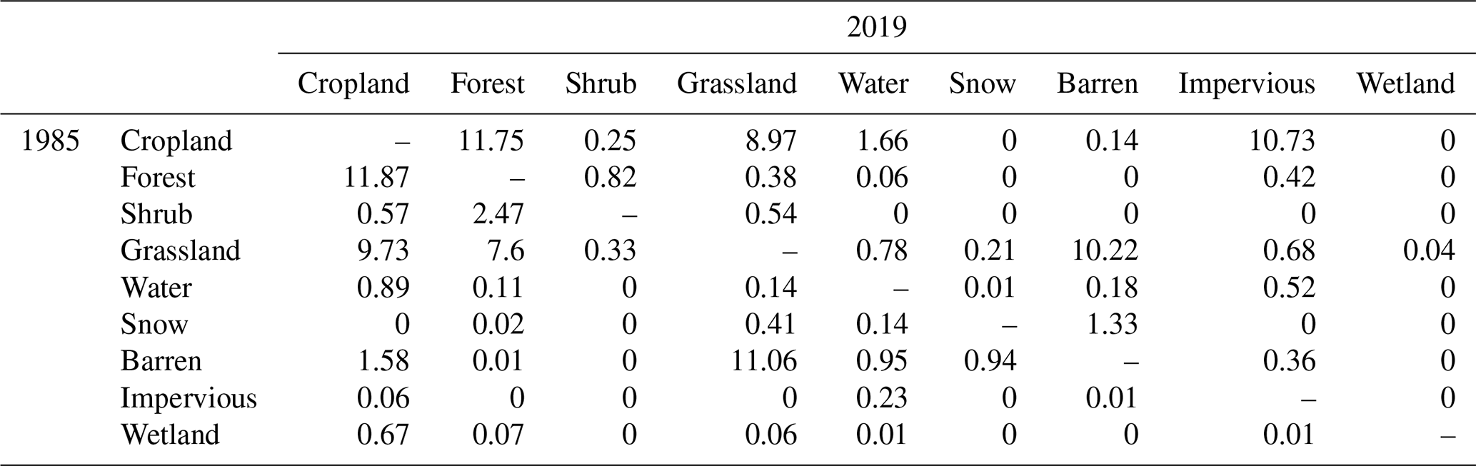
In addition to depicting the temporal trends, CLCD data can further reveal LC conversions, which are also important to global change studies. Therefore, we analysed the major LC conversions in China from 1985–2019 (Table 5). Overall, cropland loss accounted for the highest proportion among all conversions (33.50 %), followed by the grassland loss (29.55 %). The main conversion directions of cropland were the impervious area (32.03 %) and forest (35.07 %), reflecting the unprecedented urbanization process in China (Fig. 13b and i) and the Gain for Green project (Fig. 13h), respectively. Grassland (38.35 %) and forest (46.79 %) were the main sources converted to cropland (Table 4), indicating the reclamation in the northeast (Fig. 13c) and northwest China (Fig. 13g and e), respectively. Meanwhile, the interconversion between barren and grassland was also found (Liu et al., 2020a). Additionally, afforestation was also a major cause (25.72 %) of grassland loss. A total of 84.36 % of the impervious area gain came from cropland, which can be seen in Fig. 4 (e.g. North China Plain and eastern China). A total of 17.3 % of the water gain stemmed from the barren and grassland classes (e.g. Fig. 13a), which were closely associated with the rapid lake expansion in the Tibetan Plateau. The accelerated glacier melts and increased precipitation expanded those lakes (Lutz et al., 2014; Song et al., 2014). It was noteworthy that about 4 % of the impervious area originated from water (Fig. 13a), while 48.11 % of the water loss was induced by the reclamation, which has been a common phenomenon in the middle and lower Yangtze drainage region (Du et al., 2011). Lake shrinkage caused by the reclamation and urban sprawl in such regions has triggered some problems concerning the water resource management and flood relief (Hou et al., 2020; Xie et al., 2017). In particular, Fig. 13j demonstrated the conversion of barren to grassland in the Mu Us Desert of Yulin city, where green area has increased significantly over the past few decades due to several ecological restoration projects implemented by the government (Wang et al., 2020; Xiu et al., 2018). Overall, the CLCD shows great potential to reveal the human impact on LC changes under the condition of climate change and also demonstrates the promising applications in environment change studies.

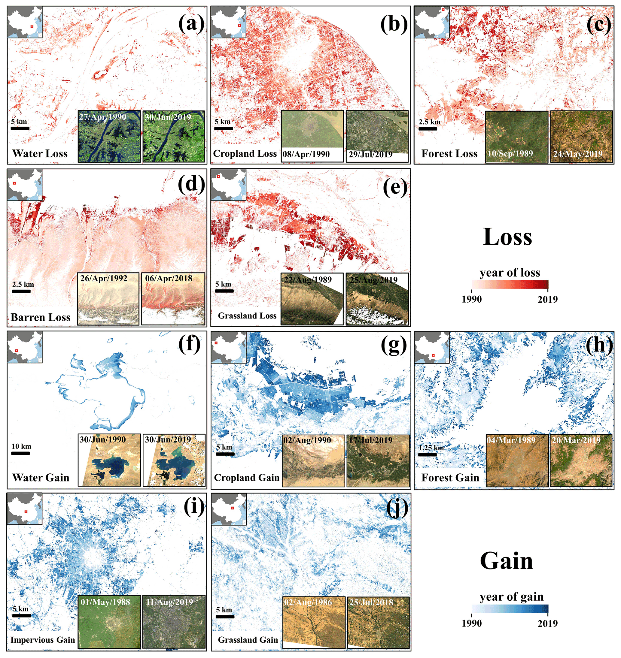
Figure 13 Typical land cover changes and conversions observed in China from 1985 to 2019: (a) lake shrinkage in Wuhan city (30.543703^∘ N, 114.296992^∘ E); (b) cropland loss due to the urbanization in Shanghai city (31.214542^∘ N, 121.490796^∘ E); (c) deforestation induced by reclamation in northeast China (49.627007^∘ N, 125.029041^∘ E); and (d) bare land converted to grassland in the Qira oasis, located at the southern fringe of the Taklamakan Desert (36.237807^∘ N, 81.215592^∘ E). The illustration is of Landsat images with false-colour combination (red: NIR, green: red, blue: green) to enhance the grassland; (e) grassland loss due to the reclamation in northwest China (43.575843^∘ N, 80.987817^∘ E); (f) Siling Co Lake (also known as Siling Lake) expansion in the Tibetan Plateau (31.793826^∘ N, 89.057216^∘ E); (g) reclamation in the Aksu Prefecture (40.593062^∘ N, 81.048109^∘ E); (h) afforestation in Yunnan Province (26.518645^∘ N, 103.613297^∘ E); (i) expansion of Chengdu city (30.666955^∘ N, 104.068452^∘ E); (j) grassland gain in the Mu Us Desert, Yulin city (38.509526^∘ N, 109.660052^∘ E).

4.4 Limitations and future work

CLCD enables fine-scale annual LC monitoring over China by combining long-term 30 m Landsat archive and cloud-based geospatial analysis platform. One of the major limitations to CLCD is the uneven spatial and temporal coverage of Landsat 5. As the only operational platform prior to 1999, Landsat 5 had no on-board storage and lost its relay capability in 1992 (Wulder et al., 2016). Thus, data transmission was limited to the line of sight of the international receiving stations (Loveland and Dwyer, 2012). Courtesy of the Landsat Global Archive Consolidation (LGAC) initiative (Wulder et al., 2016), old acquisitions performed by these international receiving stations were continuously recovered to an accessible global archive. Moreover, Landsat 5 followed a commercial pre-order acquisition plan before 1990, which further limited its availability before 1990 (Loveland and Dwyer, 2012; Pekel et al., 2016). The year of the first Landsat 5 acquisition in China varies significantly. For instance, the images were generally available over northern China around 1986 but were not available in the northwest until 1988 (Fig. S1). Therefore, we used all Landsat SR captured before 1990 to generate the CLCD of 1985 to minimize the influence induced by the availability of Landsat 5. As the Landsat archive enriches through the commissioned platforms (i.e. Landsat 7 and 8) and the LGAC, we will be able to extend the temporal coverage of the CLCD. In addition, the Multispectral Scanner System (MSS) on board Landsat 1–5 provides four spectral bands at 60 m spatial resolution. Thus, future attempts would backdate the LC monitoring to 1970s by incorporating Landsat MSS. On the other hand, there are multiple sources of data from platforms orbiting concurrently with the Landsat satellites. These data can be further employed to update and strengthen the CLCD, such as the Sentinel-2 satellites equipped with red-edge bands (20 m) and the Sentinel-1 satellites (10 m) that measure the dielectric properties and roughness. The overarching objective of this research, however, is to generate a long-term annual LC dataset for China. To this aim, Landsat images are more appropriate due to their fine spatial resolution and long-term time span.

5 Data availability

The CLCD product generated in this study is available in the public domain at https://doi.org/10.5281/zenodo.4417810 (Yang and Huang, 2021). The CLUDs were provided by the Resource and Environment Science and Data Center (available at https://www.resdc.cn/DOI/doi.aspx?DOIid=54, last access: 6 August 2021). Landsat SR, SRTM, GSW(v1.2), GFC(v1.7) and MCD12Q1 were acquired from the Google Earth Engine (available at http://code.earthengine.google.com, last access: 6 August 2021). ESACCI_LC was provided by the European Space Agency climate office (available at http://climate.esa.int/en/projects/land-cover, last access: 6 August 2021). Geo-Wiki test samples were obtained from the reference campaign (available at https://doi.org/10.1594/PANGAEA.869680, Fritz et al., 2016). The GlobeLand30 and GAUD were downloaded from the website of the National Geomatics Center of China (available at http://www.globallandcover.com/, last access: 6 August 2021) and Sun Yat-sen University (available at https://doi.org/10.6084/m9.figshare.11513178.v1, Huang, 2020). FROM_GLC, GLCVSS and GAIA were assessed from the Tsinghua University (available at http://data.ess.tsinghua.edu.cn, last access: 6 August 2021). The GISA was provided by the Institute of Remote Sensing Information Processing at Wuhan University (available at http://irsip.whu.edu.cn, last access: 6 August 2021).

6 Conclusion

LC is a fundamental parameter for environment and climate change studies. Rapid economic and population growth in China over the past few decades has tremendously altered its land cover (LC). Therefore, sequential and fine-resolution LC monitoring of China is important to implement informed and sustainable management. While the LC monitoring via satellites is increasingly recognized, fine-resolution annual LC and its dynamics in China via the remote sensing approach have rarely been investigated in the current literature. Therefore, to better understand the LC changes in China, we generated the first Landsat-derived annual China land cover dataset (CLCD) from 1990–2019 based on the GEE platform. The CLCD has higher spatial resolution and longer temporal coverage with regard to the existing annual LC products (i.e. MCD12Q1 and ESACCI_LC). The overall accuracy of CLCD reached 79.31 % based on 5463 independent test samples. In addition, assessment using 5131 third-party validation samples showed that the overall accuracy of CLCD exceeded that of MCD12Q1, ESACCI_LC, FROM_GLC and GlobeLand30. The accuracy and reliability of CLCD was further validated by comparison with Landsat-derived thematic datasets. The CLCD-based dynamic analysis revealed temporal trends and patterns of LC conversions in China, such as expansion of impervious surface and water, cropland reduction, forest increment, and grassland loss. We also found several significant LC conversions, such as the conversion of cropland to forest and the impervious, barren loss induced by grassland gain, grassland loss caused by the reclamation and afforestation, and water loss resulting from cropland sprawl, signifying the rapid urbanization as well as a series of ecological projects in China.

Annual LC information is important for environmental and climate change studies. The CLCD provides a fine-scale view of LC and its long-term changes in China at 30 m resolution. As there are increasing environment and climate modelling studies using the annual LC dataset, CLCD can provide an important reference for national or regional modelling studies. The CLCD, combined with other data (e.g. water cycle data), will allow for more comprehensive characterization of environment and climate changes.