the Creative Commons Attribution 4.0 License.
the Creative Commons Attribution 4.0 License.
 | 29 Jul 2021
African anthropogenic emissions inventory for gases and particles from 1990 to 2015
Catherine Liousse
Eric-Michel Assamoi
Thierno Doumbia
Evelyne Touré N'Datchoh
Sylvain Gnamien
Nellie Elguindi
Claire Granier
Véronique Yoboué
There are very few African regional inventories providing biofuel and fossil fuel emissions. Within the framework of the DACCIWA project, we have developed an African regional anthropogenic emission inventory including the main African polluting sources (wood and charcoal burning, charcoal making, trucks, cars, buses and two-wheeled vehicles, open waste burning, and flaring). To this end, a database on fuel consumption and emission factors specific to Africa was established using the most recent measurements. New spatial proxies (road network, power plant geographical coordinates) were used to convert national emissions into gridded inventories at a 0.1∘ × 0.1∘ spatial resolution. This inventory includes carbonaceous particles (black and organic carbon) and gaseous species (CO, NOx, SO2 and NMVOCs) for the period 1990–2015 with a yearly temporal resolution. We show that all pollutant emissions are globally increasing in Africa during the period 1990–2015 with a growth rate of 95 %, 86 %, 113 %, 112 %, 97 % and 130 % for BC, OC, NOx, CO, SO2 and NMVOCs, respectively. We also show that Western Africa is the highest emitting region of BC, OC, CO and NMVOCs, followed by Eastern Africa, largely due to domestic fire and traffic activities, while Southern Africa and Northern Africa are the highest emitting regions of SO2 and NOx due to industrial and power plant sources. Emissions from this inventory are compared to other regional and global inventories, and the emissions uncertainties are quantified by a Monte Carlo simulation. Finally, this inventory highlights key pollutant emission sectors in which mitigation scenarios should focus on. The DACCIWA inventory (https://doi.org/10.25326/56, Keita et al., 2020) including the annual gridded emission inventory for Africa for the period 1990–2015 is distributed by the Emissions of atmospheric Compounds and Compilation of Ancillary Data (ECCAD) system (https://eccad.aeris-data.fr/, last access: 19 July 2021). For review purposes, ECCAD has set up an anonymous repository where subsets of the DACCIWA data can be accessed directly through https://www7.obs-mip.fr/eccad/essd-surf-emis-dacciwa/ (last access: 19 July 2021).
- Article
(1218 KB) - Full-text XML
-
Supplement
(751 KB) - BibTeX
- EndNote


According to the UN (2015) report, World Population Prospects: The 2015 Revision, Africa is expected to account for more than half of the world's population growth between 2015 and 2050. This rapid increase in population is accompanied by a dramatic increase in anthropogenic emissions of atmospheric pollutants as shown in Liousse et al. (2014).
Pollutant concentration measurements carried out during the POLCA (POLlution des Capitales Africaines) project (Liousse and Galy-Lacaux, 2010) have shown that African urban areas such as Bamako (Mali) and Dakar (Senegal) are already highly polluted and affect the population's health (Doumbia et al., 2012; Val et al., 2013) and therefore the economy of the region. Measurements recently performed as part of the DACCIWA (Dynamics-aerosol-chemistry-cloud interactions in West Africa) program for Cotonou (Benin) and Abidjan (Cote d'Ivoire) also show that PM2.5 concentrations are 2 to 10 times higher than the WHO standards (Adon et al., 2020; Djossou et al., 2018; Evans et al., 2018). The same results were also observed in Dakar (Dieme et al., 2012). If no measures are taken, air pollution in Africa will worsen since emission regulations have yet to be implemented on the continent (Liousse et al., 2014).
An accurate estimation of anthropogenic emission inventories is fundamental for models of air quality and climate change, as well as for the development of control and mitigation strategies. Emission inventories are commonly constructed using a bottom-up approach where available statistics on fuel combustion for anthropogenic sources (e.g., traffic, industry, residential combustion) are combined with representative emission factors. Many of the inventories that exist today are at the global scale and do not contain detailed information specific to Africa. Such global inventories (Bond et al., 2004; Junker and Liousse, 2008; Granier et al., 2011; Smith et al., 2011; Klimont et al., 2013, 2017; Hoesly et al., 2018a) have been used for air quality and climate modeling in Africa (Deroubaix et al., 2018; Haslett et al., 2019).
The few regional inventories that have been published for Africa such as Liousse et al. (2014) for combustion sources and Assamoi and Liousse (2010) for two-wheeled vehicles have shown that significant uncertainties still remain on fuel consumption, emission factors and spatial distribution of emissions in Africa (e.g., there is a lack of reliable statistics on national activity data and emission factor specific to the sources considered; population density is used as a default spatialization proxy for all sectors). These previous studies indicate that some important sources such as waste burning and flaring sources are not well represented. It is therefore a challenge for policy makers to identify specific emission sources in Africa that should be considered as targets for designing effective pollution control regulations and mitigation strategies.
This paper presents a comprehensive, consistent and spatially distributed new inventory for Africa, which provides emissions of particles, i.e., black carbon (BC) and organic carbon (OC), and of gaseous compounds, carbon monoxide (CO), nitrogen oxides (NOx), sulfur dioxide (SO2) and non-methane volatile organic compounds (NMVOCs). This inventory covers the 1990–2015 period and considers the main anthropogenic emissions sources specific to Africa, such as open waste burning, charcoal making, flaring emissions as described in Doumbia et al. (2019) and two-wheeled vehicles emissions as described in Assamoi and Liousse (2010), in addition to traffic, domestics fires, industries and power plants. It takes into account the new emission factors reported by Keita et al. (2018).
Section 2 describes the methodology and data sources selected for the different emission sources. The results for sectoral emissions, spatial distributions and emission trends are presented in Sect. 3, which also includes a comparison with other studies together with a discussion on uncertainties.
The quantification of biofuel and fossil fuel emission inventories from 1990 to 2015 uses a bottom-up methodology based on the relationship
where i, j and k represents the pollutant, fuel and sector, respectively. E represents the emission of pollutant (i), EF is the emission factor (grams of pollutant per kilogram of burned fuel), CE is the efficiency of combustion and C is the annual fuel consumption in kilotons (kt). Note that this methodology follows the work of Junker and Liousse (2008) and Liousse et al. (2014). Mean CE values obtained by Keita et al. (2018) and typical for a mix of smoldering and flaming combustion conditions have been used for solid biofuels (e.g., 0.84 for fuelwood, 0.83 for charcoal use and 0.76 for charcoal making). For liquid fuels (kerosene, gasoline, diesel and liquefied petroleum gas) and natural gas, we chose CE = 1. Details regarding improvements in the representation of sectors, emission factors, etc. are given in the following sections. In addition, two new main emissions sources have been addressed, i.e., flaring and open solid waste burning.
2.1 Method for biofuel (BF) and fossil fuel (FF) emissions
2.1.1 BF and FF consumption database for 1990–2015
Fuel consumption (FC) datasets used for this regional inventory are obtained from three sources: (a) the United Nations Statistics Division (UNSTAT) database (http://data.un.org/Explorer.aspx, last access: 19 July 2021), (b) the International Energy Agency (IEA) database (https://www.iea.org/data-and-statistics/data-tables?, last access: 19 July 2021) and (c) local authorities in African countries. The UNSTAT fuel consumption database for African countries provides details for 54 countries for the years 1990 to 2015. This FC database contains information for 22 different fuels and is available by country, fuel and sector. The IEA fuel consumption database provides statistics for 28 African countries (all other countries (26) are gathered together) by fuel type and sector as in the UNSTAT database. The data originate from similar sources such as country reports, even though consumption totals are often different. The National FC database is issued by SIE (Système d'Informations Energétiques), which is a regional organization based on UEMOA (Union Economique et Monétaire Ouest Africain) countries that collects energy data from national organizations in these countries. Each year, SIE provides an annual energy statistics report that provides a comprehensive overview of the current energy situation in each country, as well as its evolution during the past years.
The FC dataset was first analyzed in detail country by country from 1990 to 2015 using the different data sources mentioned above. We found that the SIE values are on the same order of magnitude as those of IEA and UNSTAT databases, but they are incomplete. Consequently, the present work inventories are based on the UNSTAT database, which is the most complete. For cases in which there is a discontinuity in the time series for a particular country (i.e., unexplained jumps in the FC trend, missing years, etc.), the data are complemented by the IEA or SIE database when available.
FC data are then grouped into five sectors: residential combustion sources (wood, charcoal, charcoal making, etc.), industrial, power plant, traffic and other sectors including commercial, agricultural and forestry machinery. Details are retained for the four sub-sectors within the traffic sector (road, rail, domestic navigation and aviation).
The UNSTAT fossil fuel (FF) consumption database does not mention two-wheeled (TW) vehicle consumption specifically, though this is a common and highly polluting source in Africa. Previous work has shown that TW vehicles in countries neighboring Nigeria, which is Africa's largest producer and exporter of crude oil, use mainly smuggled fuel (Assamoi and Liousse, 2010). Our estimation of the number of TW vehicles and their fuel consumption is based on the work of Assamoi and Liousse (2010). Assamoi and Liousse (2010) estimated the number of TW vehicles for 16 countries in Western and Middle Africa for the year 2002 and 2005. This database was completed using the Demographic Health Surveys reports (DHS) (Corsi et al., 2012) statistical data for nine countries with non-negligible TW vehicle numbers (i.e., when the consumption of the TW fleet is more than one-tenth of the country's gasoline consumption) and for which Assamoi and Liousse (2010) do not provide data. Finally, we estimate TW vehicle numbers per year for the entire study period (1990–2015), based on linear extrapolation techniques, using Assamoi and Liousse (2010) and DHS values. Fuel consumption for TW vehicles is also calculated based on Assamoi and Liousse (2010). For the whole period 1990–2015, we use the mean values obtained from minimum and maximum assumptions given by this paper for TW vehicle characteristics (6 as the number of traffic days, 1.875 L as daily consumption for taxis and 0.75 L for private use only, and 754 kg m−3 as fuel density). TW vehicles are indeed used for public transportation in addition to private use in six Western and Middle African countries (Benin, Cameroon, Chad, Niger, Nigeria and Togo).
2.1.2 Emission factors (EFs)
Emission factors are dependent on fuel type, activity, technology and emission reduction regulations. However, in Africa, information on technology and regulations is not available for each fuel/activity and country. To take into account this limitation, our methodology is based on a “lumping” procedure designed to manage available experimental data and account for the main factors of variability. Technologies and regulations are assumed to be country-dependent, and all 54 African countries are classified into two groups, developing countries (1) and semi-developed countries (2), based on their gross national product per capita (GDP) (World Bank, 2005), for which different EFs are assigned. Twelve African countries are considered to be semi-developed countries, including South Africa, Eswatini, Morocco and Algeria, and the other 42 countries are classified as developing countries. Table 1 presents the EF values for black carbon (BC), primary organic carbon (OC) and gaseous compounds, i.e., carbon monoxide (CO), non-methane volatile organic compounds (NMVOCs), nitrogen oxides (NOx) and sulfur dioxide (SO2) for each country type and the main anthropogenic sources.
Table 1BC, OC, CO, NOx, SO2 and NMVOCs EFs for the main anthropogenic sources, for different fuels (AV: aviation gasoline, JF: jet fuel, DL: diesel, MO: motor gasoline, RF: residual fuel oil, FW: wood, CH: charcoal, and CHM: charcoal making), type of country (1: semi-developed, 2: developing) and activities sectors (DAV: domestic aviation, DNAV: domestic navigation, RAIL: rail traffic, ROAD: road traffic, and D: residential combustion).
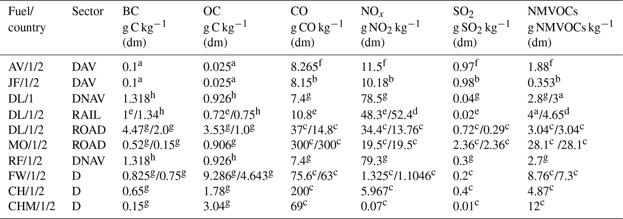
a Wei et al. (2008). b Kurniawan and Khardi (2011). c Liousse et al. (2014). d eea/1.A.3.C Railways/tier 1. e TRANSFORM, deliverable D1.2.5, type report on railway emission factor. f IPCC, Reference Manual (Eggleston et al., 2006). g Keita et al. (2018). h IIASA, GAIN EF.
BC and OC EFs for motor gasoline, diesel oil, two-wheel vehicles, wood burning, and charcoal burning and making are taken from Keita et al. (2018) for developing countries. For semi-developed countries, the ratios of EFs between semi-developed and developing countries in Africa for specific sources as discussed in Liousse et al. (2014) are used to estimate the EFs for this inventory.
BC and OC EFs for the other sources (i.e., industries, energy, etc.), as well as EFs for the other species (CO, NOx, NMVOCs, SO2), are provided by Liousse et al. (2014), with the exception of the non-road traffic sub-sectors. For rail and domestic aviation using diesel (DL), aviation gasoline (AV) and jet fuel (JF), EFs for developing countries are taken to be the highest value found in the literature as presented in Table 1. For these sub-sectors, the same EF is used for semi-developed and developing countries.
It should be noted that, as reported in Keita et al. (2018), new EF values for BC and OC for motor gasoline, diesel oil, and wood burning are higher than those reported by Liousse et al. (2014) (for example for motor gasoline by a factor of 1.5 and 4 respectively for OC and BC) and slightly lower in the case of charcoal burning, charcoal making and two-wheel vehicles (for example for charcoal making by a factor of 0.8 and 0.9 respectively for OC and BC).
2.2 Method for open waste burning (WB) emissions
The inventory for open waste burning has been built following the IPCC guidelines (chap. 2 and 5 available at https://www.ipcc-nggip.iges.or.jp/public/2006gl/vol5.html, last access: 19 July 2021) for the estimation of greenhouse gases (GHGs): it includes open residential burning and dump waste burning. This inventory does not include the waste burning practices in incinerators or modern combustion systems, which are already accounted for in the industrial sector.
Open waste burning is estimated using the following expression:
where WB is the amount of solid waste that is burned residentially and in uncontrolled dumps, and EFi is the emission factor of pollutant i. EF values for BC and OC are provided by Keita et al. (2018), from Akagi et al. (2011) and from Wiedinmyer et al. (2014) for the other species (NOx, NMVOCs, CO and SO2).
For each African country, the WB amount is estimated following Sect. 5.3.2 of the IPCC Guidelines for National GHG Inventories (Eggelston et al., 2006), which states
where P is the national population given by the World Bank database (http://data.worldbank.org/indicator, last access: 2 November 2016) and MSWp is the mass of annual per capita waste production taken from Wiedinmyer et al. (2014). The default value of 0.6 recommended by IPCC is used for Bfrac: this is the fraction of waste available to be burned that is actually burned. Pfrac is the fraction of the population assumed to burn some of their waste either near their residence or in uncontrolled dumps. Values for Pfrac used in our calculations are taken from Wiedinmyer et al. (2014). Pfrac is assumed to be based on national income status, urban versus rural population, and waste collection practices. In Africa, Pfrac may be considered to be 100 % following Wiedinmyer et al. (2014). This value is the value obtained for countries with low income, low middle income and upper middle income, following the classification of the World Bank (http://data.worldbank.org/country, last access: 19 July 2021). In this context, data for semi-developed countries are not available. Therefore, an overestimation of waste burning practices may be expected in some countries (e.g., South Africa, Morocco, Egypt). However, currently no data exist to avoid this overestimation.
Note that it is possible to distinguish waste burning emissions which occur near the residence from those in uncontrolled dumps. Such practices are highly different in rural and in urban areas. WB can also be calculated using the following equation:
where WBR and WBU represent waste burning in rural and urban areas, respectively, and are defined by
In Africa, the rural population is assumed to have no organized waste collection; therefore, in rural areas (PfracRes)R linked to residential burning is assumed to be equal to 100 %, whereas (PfracDump)R linked to uncontrolled dumps is 0 %. In urban areas, (PfracDump)U is country-dependent: for example, the fraction of uncollected waste is 0.77, 0.30, 0.40 and 0.76 for Benin, Côte d'Ivoire, Ghana and Nigeria, respectively (Wiedinmyer et al., 2014). Therefore, in Benin for example (PfracRes)U is assumed to be equal to 77 % and (PfracDump)U is 23 %. Rural (Prural) and urban (Purban) populations are provided by the World Bank database (http://data.worldbank.org/indicator). Rural/urban distinction for estimating WB emissions is an important improvement to our inventory, providing details at the local and regional levels which are missing in global inventories.
2.3 Spatial distribution of the fossil fuel, biofuel and waste burning sources
The final step in the development of the inventory is the disaggregation of the country-level emission totals to the African gridded domain at 0.1∘ × 0.1 ∘ latitude–longitude resolution using appropriate spatial proxies for each sector. Three types of geographic information system (GIS) datasets at a resolution of 0.1∘ × 0.1∘ are used here for disaggregation: (1) 2010 population density given by the Center for International Earth Science Information Network (CIESIN; Gridded Population of the World Future Estimate: GPWFE), (2) African country road networks based on gridded emission files from EDGAR traffic inventory (Janssens-Maenhout et al., 2011) and (3) African power plant networks given by Africa infrastructure (https://powerafrica.opendataforafrica.org/, last access: 19 July 2021). These spatial allocation proxies are used as follows: (1) road networks are used for road traffic emissions; (2) geographical coordinates of power plants are used for energy production emissions; and (3) the population density grid is used for residential combustion sources, industries and waste burning. In the future, we plan to use gridded rural and urban population densities to better disaggregate waste burning and residential emissions in Africa.
2.4 Method for flaring emissions
Flaring emissions are taken from the inventory developed by Doumbia et al. (2019) for the years 1994 to 2015 using the following equation:
where EXflaring is the emission rate of a pollutant X (kiloton) and GFvolume is the volume of gas flared in billions of cubic meters (bcm). Yearly averages GFvolume by country for the period 1994–2010 are taken from the National Oceanic and Atmospheric Administration (NOAA) (http://ngdc.noaa.gov/eog/dmsp/, last access: 19 July 2021) DMSP (Defense Meteorological Satellite Program) dataset. No data exist for the years 1990–1993. For the period 2012–2015, estimations of GFvolume are based on Visible Infrared Imaging Radiometer Suite (VIIRS) satellite data (Elvidge et al., 2015) and are spatially distributed based on the DMSP 2011 product. GFvolume for 2011 is estimated from 1994–2010 trends and from the 2012–2015 time series as the 2011 DMSP data cannot be used due to an orbital degradation that led to solar contamination.
XEF is the emission factor (EF) for species X in g kg−1 of fuel burned, and ρ is the density of the fuel gas. Typically, the density of the fuel (natural gas) varies between 0.75 and 1.2 kg m−3 depending on the fraction of heavy hydrocarbons present in the fuel (US Standard Atmosphere, 1976). In this inventory, we assume a gas density of 1.0 kg m−3 for converting the volume of the associated gas to mass (E&P Forum, 1994). EFs for various species (CO, NOx, NMVOCs, SO2, OC and BC) are detailed by Doumbia et al. (2019), and they show a large range of uncertainties. We use here the mean EF value given in the Doumbia et al. (2019) paper.
Spatial disaggregation is achieved by overlapping layers of maps including DMSP nighttime light images, gas flare areas, world maritime boundaries and total gas flare volume per country based on a geographic information system (ArcGIS software). The final layer is gridded at a 0.1∘ × 0.1∘ horizontal resolution.
3.1 Temporal trends of African emissions
Figure 1 shows the time series of BC emissions for fossil fuel (FF), biofuel (BF), open waste burning (WB) and flaring sources in Africa from 1990 to 2015. The BC emissions increase by 46 %, 67 % and 43 % for the fossil fuel (FF), biofuel (BF) and open waste burning (WB) sources, respectively, during this time period. This change is mainly due to anthropogenic activity increases linked to population growth. Africa's population has grown by 2.5 % yr−1 over the past 20 years, corresponding to a roughly 64 % increase over the period 1990–2015, which is of the same order of magnitude as the increase in biofuel emissions. Biofuel emissions have increased at a higher rate than other sources due to an increase in low-income population in sub-Saharan Africa, where biomass constitutes about 80 % of the total energy consumption (Ozturk and Bilgili, 2015).
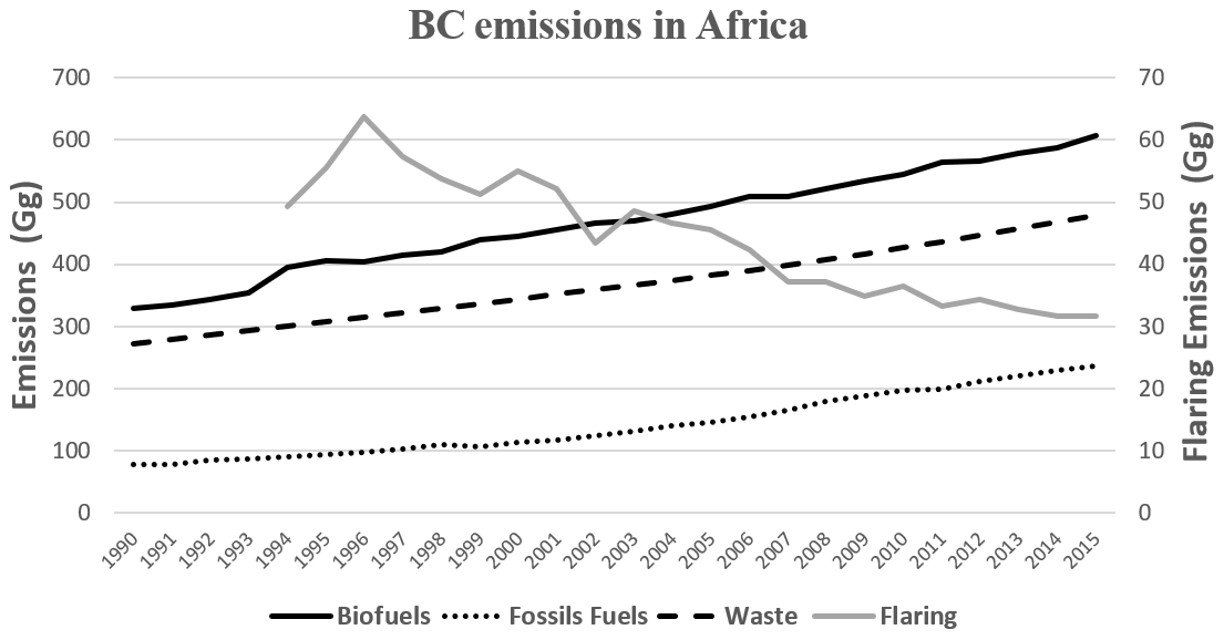
Figure 1Time series of BC emissions in Africa for fossils fuels, biofuels, open waste burning and flaring.
Unlike FF, BF and WB, BC emissions from flaring are decreasing (55 % from 1994 to 2015) due to the actions of the Global Gas Flaring Reduction initiative (GGFR). In 1994, BF, FF, WB and flaring contributions to total anthropogenic BC emissions were roughly of the order of 47 %, 11 %, 36 % and 6 %, whereas in 2015 such values are 45 %, 17 %, 35 % and 2 %, respectively. Increases in the contribution from FF can be explained by increases in the traffic fleet and industrialization.
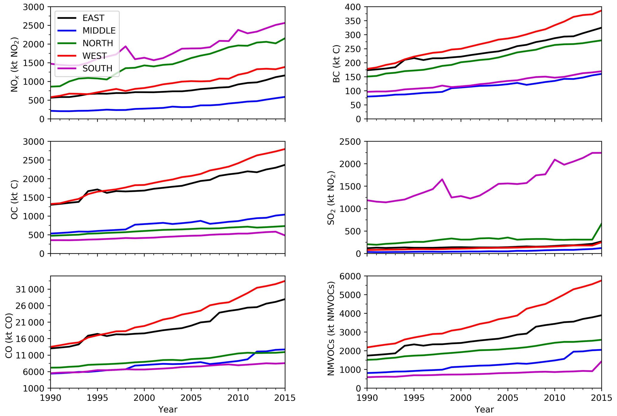
Figure 2Time series of regional emission estimates of BC, OC, NOx, CO, SO2 and NMVOCs for fossils fuel, biofuel and waste burning sources.
Figure 2 shows the trends in pollutant emissions in five subregions of Africa (Northern, Eastern, Western, Middle and Southern Africa) for the main sources (fossils fuels, biofuels and waste burning) during the period 1990–2015. The list of countries included in these five regions is given in Table S1 of the Supplement. In Africa, all pollutant emissions are generally increasing over the period 1990–2015 at a growth rate of 95 %, 86 %, 113 %, 112 %, 97 % and 130 % for BC, OC, NOx, CO, SO2 and NMVOCs compared to 1990, respectively. Except for OC, emissions of all pollutants have nearly doubled between 1990 and 2015.
The regional contributions of BC, OC, CO and NMVOCs show similar patterns, with the highest values for Western Africa, Eastern Africa and Northern Africa (except for OC, for which Middle Africa emissions are higher than Northern Africa emissions). Southern Africa emits more SO2 and NOx than all the other African regions, followed by Northern Africa. This is due to their large amount of industrial activities compared to the other regions of Africa.
Analysis of BC emissions by region indicate that the highest emitting region is Western Africa with 0.18 Tg (26 %) in 1990 and 0.39 Tg (29 %) in 2015 followed by Eastern Africa with 0.17 Tg (26 %) in 1990 and 0.33 Tg (25 %) in 2015, Northern Africa with 0.15 Tg (22 %) in 1990 and 0.28 Tg (21 %) in 2015, Southern Africa with 0.10 Tg (14 %) in 1990 and 0.17 Tg (13 %) in 2015, and Middle Africa with 0.08 Tg (12 %) in 1990 and 0.16 Tg (12 %) in 2015. Western Africa's contribution to BC emissions shows the fastest growth (26 % to 29 %) compared to the other regions. The highest rate of increase in BC emissions is also observed in Western Africa (117 %) and the lowest in Southern Africa (70 %) over the period 1990–2015. This could be in part explained by the fact that the population growth rate in Africa is higher in Western Africa with a value of 2.66 % yr−1 and lower in Southern Africa with a value of 1.64 % yr−1, as shown by United Nations (2015). Furthermore, differences in BC emissions between Southern and Northern Africa regions with similar fuel consumption (for fossil fuels, biofuels and solid waste) are partly explained by the emission factors which are higher in Northern Africa, which includes more developing countries (four of seven countries) than in Southern Africa (one of five countries).
In terms of SO2 emissions, the highest emitting region is Southern Africa, which is the most industrialized region in Africa, with emissions of 1.19 Tg (73 %) in 1990 and 2.24 Tg (63 %) in 2015. Southern Africa is followed by Northern Africa, Eastern Africa, Western Africa and Middle Africa, respectively. Over the 1990–2015 period, the highest rate of increase in SO2 emissions occurred in Western Africa (224 %) followed by Middle Africa (71 %), Eastern Africa (56 %), Southern Africa (47 %) and Northern Africa (33 %), respectively. As for BC, the highest rates of increase in SO2 emissions during this period are observed in regions where the population growth rate is the highest, i.e., Western Africa (2.66 %yr−1), Middle Africa (3.10 % yr−1) and Eastern Africa (2.71 % yr−1), whereas the lowest rates are found where the population growth rate is the lowest, i.e., Southern Africa (1.64 % yr−1) and Northern Africa (1.87 % yr−1).
3.2 Focus on the year 2015
Figure 3 shows the spatial distribution of BC and NOx emissions in 2015 for the fossil fuel, biofuel, waste burning and flaring sources. As given in Table 2, which shows the contribution of each of these sources to the total emissions for BC, OC, NOx, SO2, CO and NMVOCs in 2015, total BC and NOx emissions are 1.35 Tg C and 7.90 Tg NO2, respectively. Emission densities are generally the highest along the Gulf of Guinea and in the east and south of Africa. Table 2 also indicates that for Africa, residential combustion is the major source of carbonaceous particles for BC (40 %) and OC (77 %). It is also the main source of CO and NMVOCs with a contribution of 72 % and 53 %, respectively. Open waste burning is the second most important source of BC, OC and NMVOCs, representing 35 %, 15 % and 22 % of the total, respectively. The energy sector is the major source of SO2 and NOx emissions, which constitute 54 % and 29 % of the total, respectively. For NOx emissions, the energy sector is followed by the traffic sector (26 %), whereas industry is the second largest contributor to SO2 emissions (32 %).

Figure 3Spatial distribution of total anthropogenic BC and NOx emissions in 2015.
Table 2Sectoral emissions of carbonaceous particles and combustion gases in 2015 in Africa in Gg yr−1.
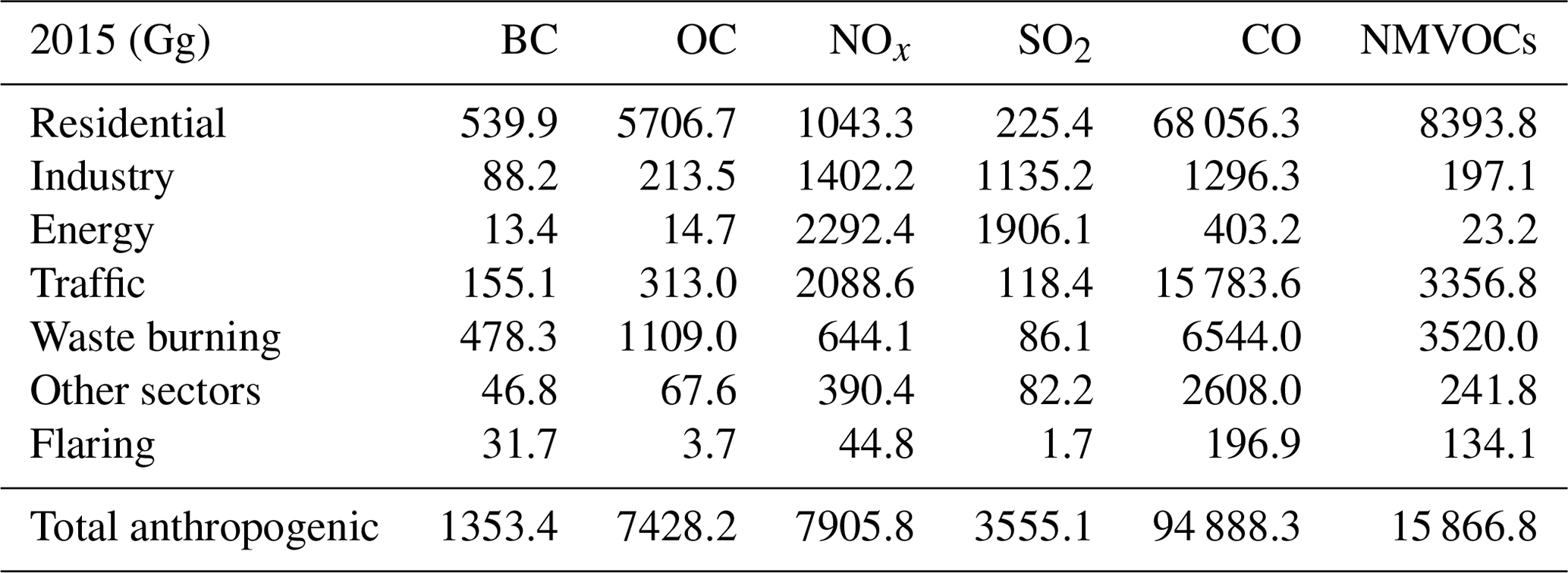
The regional contribution from each sector is presented in Fig. 4. The residential sector contributes to more than 50 % of BC emissions in Eastern and Western Africa and just under 50 % in Middle Africa (Fig. 4a) for the year 2015. In Southern and Northern Africa, it contributes to less than 25 % and 10 % of the total BC emissions, respectively. In these two regions, waste burning is the largest source of BC emissions, with significant contributions from the industry and traffic sources compared to Eastern and Western Africa. Waste burning is the second largest source of BC emissions in Eastern and Western Africa. For NOx, the traffic sector is the largest contributor in Western and Northern Africa, with 30 % and 41 % of the total emissions, respectively (Fig. 4b). In Eastern Africa, the residential sector (32 %) is the largest contributor of NOx emissions, followed by the traffic sector (23 %). In Southern Africa, the two largest contributors to NOx emissions are the energy (52 %) and industry (27 %) sectors, respectively.
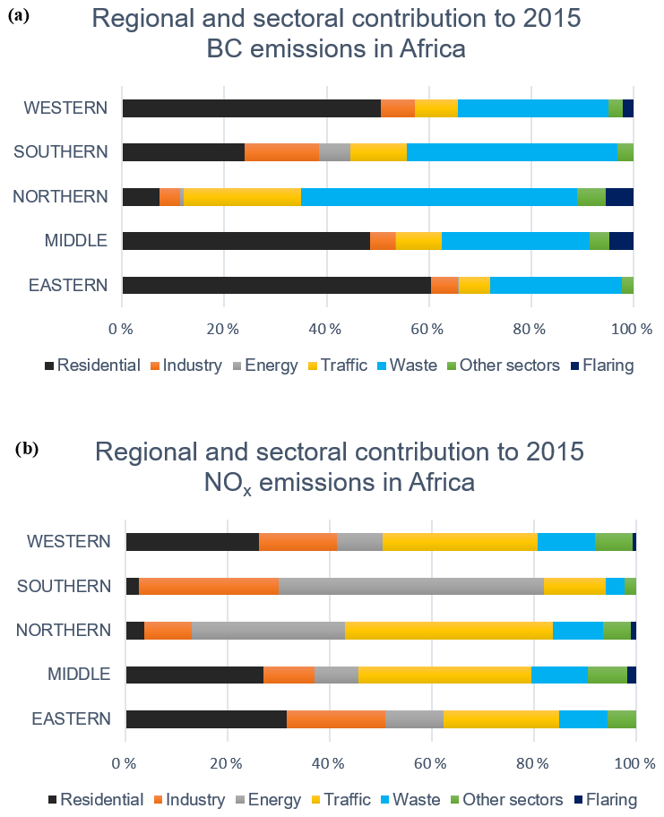
Figure 5 shows the sectoral contributions of BC emissions for a few countries in southern Western Africa (SWA) and for South Africa with different predominant sources. As previously mentioned, for countries in SWA, BC emissions are dominated by the residential sector, followed by open solid waste burning and the other sources, whose relative importance differs depending on the country. In Nigeria, industry and flaring BC emissions are much more important than in other countries in SWA. It is also interesting to see that traffic is the largest contributor to BC emissions in Benin, which can be explained by the high number of two-wheeled vehicles, which are more polluting than four-wheel vehicles. In Benin, TW vehicles represent 34 % of road traffic emissions and only 16 % in Côte d'Ivoire for example. In South Africa, waste burning is the predominant sector, contributing 42 % to the total BC emissions (18 % residentially and 24 % in dump locations), followed by the residential (24 %), industry (24 %), energy (13 %), traffic (9 %) and flaring sectors. In Côte d'Ivoire, the residential sector is the most important (58 %), followed by waste burning (26 % with 16 % residentially and 10 % in dump locations), traffic (9 %), other sectors (5 %), industry (1 %) and energy (0.1 %). In South Africa BC emissions from the waste burning sector are higher at the dump than at residences compared to Côte d'Ivoire, where there is less organized waste collection. South Africa is the country emitting the highest amount of SO2, with roughly 62 % of the total African SO2 emissions. Such an important contribution is due to coal-fired power plants with emissions in the range 1000–1500 Gg for the period 1999–2012. These numbers are in agreement with the range given by Pretorius et al. (2015), i.e., 1500–2000 Gg for the same period.
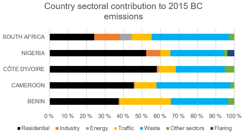
Finally, it is interesting to assess the relative importance of each type of fuel in the sectoral emissions. For BC emissions, emissions related to diesel are 7 times and 8 times higher than gasoline emissions in Côte d'Ivoire and South Africa, respectively. Similarly, wood burning leads to emissions that are about 3 times higher than charcoal burning and making in Cote d'Ivoire. SO2 emissions originate mainly from the use of coal, which constitutes 95 % of the emissions in South Africa (51 % from power plants, 31 % from industry, 4 % from the residential sector and 3 % from other sectors). This demonstrates that actions to substitute diesel by gasoline and wood by charcoal in Côte d'Ivoire would be beneficial to reduce BC emissions. In addition, replacing coal with other fuels such as natural gas would also help reduce BC and SO2 emissions in South Africa.
3.3 Comparison with previous emission inventories
We first compared the emissions provided by this inventory (DACCIWA inventory) to the inventories developed by Liousse et al. (2014) for the year 2005 and with the emissions from Marais and Wiedinmyer (2016), i.e., the DICE-Africa dataset available for 2006 and 2013. Table 3 summarizes the emissions of pollutants (BC, OC, NOx, SO2, CO and NMVOCs) for the years 2005, 2006 and 2013 for these inventories. Fossil fuel and biofuel emissions from the DACCIWA inventory are slightly lower than those given by Liousse et al. (2014) for BC (0.64 instead of 0.69 Tg), NOx (5.08 instead of 5.80 Tg) and NMVOCs (8.33 instead of 8.60 Tg), lower for SO2 (2.53 instead of 4.02 Tg), and slightly higher for OC (4.96 instead of 3.95 Tg) and CO (64.43 instead of 58.6 Tg). These differences may be explained by the use of more recent fuel consumption data and new emissions factors which are taken from direct measurements. The DACCIWA inventory also includes two major sources not considered in the Liousse et al. (2014) inventory, namely open solid waste burning and flaring sources: including these sources increases the 2005 emissions by 36 %, 33 %, 16 % and 24 % for BC, OC, CO and NMVOCs, respectively, as compared to the Liousse et al. (2014) values.
Table 3Comparison of fossil fuel and biofuel emissions between this work, Liousse et al. (2014), and Marais and Wiedinmyer (2016) inventories for the year 2005, 2006 and 2013.
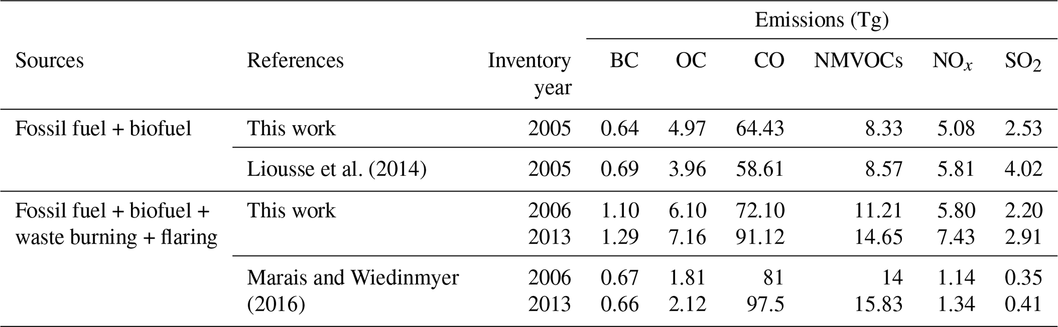
Table 3 indicates that the DACCIWA emissions of BC, NOx, OC and SO2 are at least 39 % larger than those of Marais and Wiedinmyer (2016), except for NMVOCs and CO emissions which are lower (7 %–25 %). The differences between the DACCIWA datasets and the values reported by Marais and Wiedinmyer (2016) are largely due to the use of different emission factors. A table with the sectoral EFs used in this work and in the Marais and Wiedinmyer (2016) inventories is provided in Table S2. The DICE-Africa inventory uses for example only one EF value for road traffic gathering, motor gasoline and diesel fuel. In the DICE-Africa inventory, much lower BC and OC EFs are used than in this study for the residential source: for example, BC and OC EFs in this study are respectively 5 and 7 times larger than the values used in DICE-Africa.
We also compared our inventory for Africa to emissions from the following global inventories: ECLIPSEv5a (Klimont et al., 2017), EDGARv4.3 (Janssens-Maenhout et al., 2011), CEDS (Hoesly et al., 2018b) and CEDSGBD-MAPS (McDuffie et al., 2020). These global inventories are also developed using a bottom-up methodology, where emissions are calculated as the product of IEA activity data and emission factors for combustion sources including diverse levels of details in technology and emission controls.
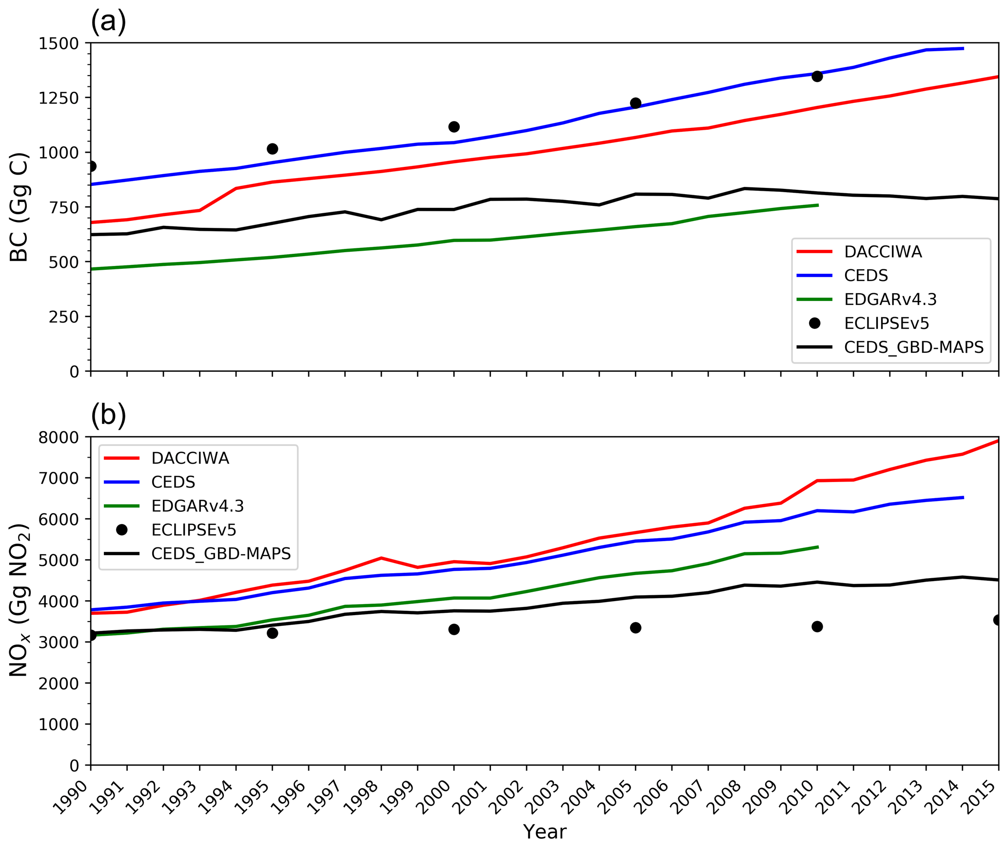
Figure 6Comparison of BC (a) and NOx (b) between DACCIWA inventory (this work) and global inventories (CEDS, CEDS_GBD-Maps, EDGARv4.3 and ECLIPSEv5 inventories).
Figure 6 shows BC and NOx emission trends from our DACCIWA inventory and the four global inventories mentioned in the previous paragraph. Emission values are indicated in Fig. 6 by colored lines except for ECLIPSEv5a, where values are indicated by dots every 5 years. There are large differences among the emissions for BC, while trends are similar. BC emissions from CEDS and ECLIPSEv5a are both slightly higher than those calculated in this work (12 % on average) over the period 1990–2014. BC emissions from EDGARv4.3 and CEDSGBD-MAPS are, however, much lower, with emissions from the DACCIWA inventory up to 37 % higher on average over the period 1990–2010. NOx emissions from the DACCIWA inventory are of the same order of magnitude as CEDS over the period 1990–2009 (difference of the order of 3 %). This difference becomes larger after 2010, where NOx emissions from the DACCIWA's dataset are about 15 % higher than from CEDS. CEDSGBD-MAPS NOx emissions are lower than the CEDS NOx emissions (on average 23 %) and DACCIWA NOx emissions (on average 27 %). For BC, the NOx emissions from DACCIWA are higher on average by 18 % compared to EDGARv4.3 over the period 1990–2010. The NOx emissions from ECLIPSEv5a are the lowest of all inventories. These differences are due to the use of different fuel and activity datasets in DACCIWA (mainly from UNSTAT) and the two global inventories (IEA), as well as differences in emission factor values used in the different inventories. The EFs used in the DACCIWA inventory are taken from direct measurements at the sources in Africa as described in Keita et al. (2018), whereas the EFs used in global inventories are largely based on measurements taken from other regions such as Europe and the US, which are often not appropriate for Africa.
A comparative analysis of sectoral BC and NOx emissions from the different emission inventories considered in Fig. 6 is performed, which provides further information on the differences between the inventories. For this comparison, we use the year 2010, which is the most recent common year for these inventories. The fugitive sector in CEDS and EDGARv4.3 inventories mainly consists of flaring emissions; in the ECLIPSEv5a and CEDSGBD-MAPS inventory, fugitive emissions are included in the energy sector. Figure 7 shows the relative contribution from each sector to BC and NOx emissions in 2010 for the DACCIWA inventory and the four global inventories. While large disparities exist between the inventories, it is clear that the residential sector is the highest contributor to BC emissions in all the inventories. The main differences in BC emissions are largely due to the residential and waste sectors. The contribution of emissions from the waste sector varies greatly among the inventories (35 %, 7 %, 5 % and 1 % for DACCIWA, CEDS, CEDSGBD-MAPS and EDGARv4.3, respectively). It should be noted that ECLIPSEv5a does not consider a waste sector. The traffic and energy sectors are the largest emitters of NOx for both the CEDS (31 % and 27 %, respectively), CEDSGBD-MAPS (18 % and 38 %, respectively) and EDGARv4.3 (34 % and 32 %, respectively) inventories. In the DACCIWA inventory, the contribution from the energy sector (28 %) is slightly larger than from the traffic sector (25 %).
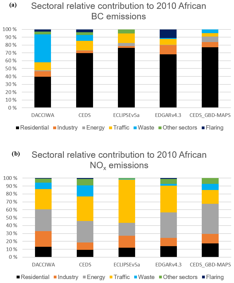
Figure 7Sectoral relative contribution for BC (a) and NOx (b) emissions in 2010 for CEDS, CEDS_GBD-Maps, ECLIPSEv5a, EDGARv4.3 and DACCIWA (this work) inventories.
We also compared OC and SO2 emission trends from our inventory and the four global inventories, as shown in Fig. S1. The DACCIWA inventory shows the highest value for OC emissions. This is mainly due to the value of the OC emission factor used for domestic fires (Keita et al., 2018), which is higher than previous values found in the literature based on measurements from other regions of the world with different wood species. In contrast to OC, SO2 emissions from DACCIWA have the lowest values compared to other inventories. This could be due to differences in activity database and to the EF used for NOx and BC emissions.
Finally, Liousse et al. (2014) have estimated the emissions of BC and OC in 2005 and 2030, using different scenarios. The authors defined the REF scenario as the state of the world for “business and technical change as usual” conditions, driven solely by basic economics. Another scenario has been proposed (called CCC*), where the introduction of carbon penalties and Africa-specific regulations are implemented to achieve a large reduction in emissions from incomplete combustion. These values are shown by the dots in Fig. S2 for the REF and CCC* scenarios. We have linearly extrapolated the DACCIWA emissions for these two species, as shown by the plain lines in Fig. S2. Our estimates for BC and OC are higher than the best-case scenario values and lower than the worst-case scenario values of Liousse et al. (2014). However, OC values are much closer to the worst-case scenario, and BC values are closer to the best-case scenario. These results demonstrate that emission mitigation measures need to be implemented urgently in Africa in order to avoid such elevated emissions in 2030.
3.4 Emission uncertainty analysis
3.4.1 Method for emission uncertainty calculation
Uncertainties in emission inventories are mainly due to the lack of information on fuel consumption and emission factors. The main challenges in the estimation of uncertainties in emissions are related to the uncertainties in input data and in the development of methods for quantifying systematic errors. In this study, we use a Monte Carlo statistical method to quantify the impact of the uncertainties in the input data such as emission factors and fuel consumption data on the emissions. A Monte Carlo simulation has been performed in order to quantify the uncertainty in emission estimates (Frey and Zheng, 2002; Frey and Li, 2003; Zhao et al., 2011). Parametric distributions and standard deviation linked to the reliability and accuracy of data introduced by fuel consumption statistics and non-national emission factors are provided in the literature (e.g., Eggleston et al., 2006; Zhao et al., 2011; Bond et al., 2004) and expert judgment. In this study, we assume that, when the coefficient of variation is less than 30 %, the distribution is normal (Eggleston et al., 2006). When the coefficient of variation is larger and the quantity is non-negative, an asymmetric lognormal distribution is assumed. The Monte Carlo method was then used to propagate these uncertainties to obtain the uncertainty on emissions for each fuel per sector. The Monte Carlo analysis consisted of selecting random values of activity and emission factor data from the respective distributions to obtain the corresponding emissions. This calculation was repeated 100 000 times to obtain the average value of the 100 000 emission values and their distributions. The standard deviations for these distributions were estimated with a 95 % confidence interval. The uncertainty on the total emission per pollutant was obtained by combining values obtained by fuel oil and by sector.
3.4.2 Uncertainty results
The uncertainties in the emission estimates are within [−35 %; +58 %], [−15 %; +20 %], [−17 %; +21 %], [−16 %; +18 %], [−14 %; +16 %] and [−17 %; +23 %] for BC, NOx, OC, CO, NMVOCs and SO2, respectively. As expected, the highest uncertainties are observed for the smallest emission values (e.g., BC). Uncertainties in biofuel activity data (20 %–100 %) are greater than those for fossil fuels (10 %–20 %) because of the absence of official markets for biofuels and consequently lower accuracy in their consumption estimates. Biofuel used in the residential sector shows the highest uncertainties for this inventory, for example with [−40 %; +101 %] and [−38 %; +171 %] for BC and NOx, respectively, with a 95 % confidence interval. For fossil fuel, the highest uncertainties are obtained for two-wheeled vehicles with [−62 %; +115 %] and [−74 %; +173 %] for BC and NOx, respectively, with a 95 % confidence interval. For two-wheeled vehicle fuels, higher uncertainties are due to the lack of statistics on the number of two-wheeled vehicles and their consumption. It should be noted that some uncertainties are not taken into account. For example, EFs were considered to be constant over the studied period, while the GDP of countries vary as well as the composition of the TW vehicle fleet (two and four stroke ratio). Waste burning emission estimates in Southern Africa assume that Southern Africa includes only developing countries. Emissions are then overestimated since the parametrizations should include characteristics of both semi-developed and developing countries. This issue is not considered in the uncertainty calculations.
Annual gridded emissions at a spatial resolution of 0.1∘ × 0.1∘ for BC, OC, CO, NMVOCs, SO2 and NOx from the residential, industry, energy, traffic, open waste burning, flaring and other sectors for the years 1990 to 2015 are provided in the NetCDF format (DACCIWA, https://doi.org/10.25326/56, Keita et al., 2020) and are available through the Emissions of atmospheric Compounds and Compilation of Ancillary Data (ECCAD) system with a login account (https://eccad.aeris-data.fr/, last access: 19 July 2021). For review purposes, ECCAD has set up an anonymous repository where subsets of the DACCIWA data can be accessed directly https://www7.obs-mip.fr/eccad/essd-surf-emis-dacciwa/ (last access: 19 July 2021).
Within the framework of the DACCIWA project, a new African emission inventory has been developed for fossil fuel, biofuel, open waste burning and gas flaring for the years 1990–2015. Emissions of BC, OC, CO, NMVOCs, SO2 and NOx are included for the residential, industry, energy, traffic, open waste burning, flaring and other sectors. These emissions are provided at a spatial resolution of 0.1∘ × 0.1∘. The inventory uses new emission factors derived from direct measurements for the main emission sources in Africa, new spatial distribution proxies and the addition of new emission sources as compared to previous regional African emission inventories.
In this paper, emissions are discussed in the context of five geographical regions in Africa. Our analysis highlights differences in the characteristics of both fuel consumption and pollutant emissions in these regions. Western Africa is identified as the highest emitting region of BC, OC, CO and NMVOCs, followed by Eastern Africa and/or Northern Africa. Southern Africa and Northern Africa are the highest emitting regions of SO2 and NOx. These differences are due to the relative contribution of emissions from different activity sectors. High SO2 and NOx emissions in Southern Africa and Northern Africa are linked to their large quantities of industrial activities and thermal power plants, whereas in regions with more developing countries (44 out of 56 African countries) such as Western or Eastern Africa, higher emissions from the domestic and traffic sectors are found.
Comparisons with other inventories reveal significant differences between both regional inventories (Liousse et al., 2014, and DICE-Africa) and global inventories. Differences with Liousse et al. (2014) are largely due to updated activity data and emission factors used in this inventory. The DICE-Africa inventory shows BC and OC emissions larger than in the DACCIWA inventory, which is mainly due to the choice of the emission factors in residential and traffic sectors. The DACCIWA emissions are within the range of three global inventories, EDGARv4.3 and CEDSGBD-MAPS (lower bound), and CEDS and ECLIPSEv5a (upper bound), depending on the species.
In addition, an estimation of the emission uncertainties has been presented. These uncertainties are due to both the lack of reliable statistics on data for the different sectors considered in the dataset as well as to the assumptions which have been made (e.g., constant EFs over the study period, less-well-known EFs for industry and flaring sources). Finally, this inventory highlights the key pollutant emission sectors which could be considered for the development of mitigation scenarios.
The supplement related to this article is available online at: https://doi.org/10.5194/essd-13-3691-2021-supplement.
SK processed the data, performed the calculations, drafted the manuscript. CL helped conceive and develop the DACCIWA inventory. CL and VY supervised the work. EMA, TD, ETN'D and SG helped obtain data and construct the inventory data files. NE and CG provided comments on emission levels compared to global inventories, helped proofread the English in an earlier version of the manuscript and made data files available through the ECCAD system. SK prepared the manuscript with contributions from all co-authors.
The authors declare that they have no conflict of interest.
Publisher's note: Copernicus Publications remains neutral with regard to jurisdictional claims in published maps and institutional affiliations.
This article is part of the special issue “Surface emissions for atmospheric chemistry and air quality modelling”. It is not associated with a conference.
This work has received funding from the European Union Seventh Framework Programme (FP7/2007-2013) under grant agreement no. 603502 (EU project DACCIWA: Dynamics-aerosol-chemistry-cloud interactions in West Africa). We thank the Emissions of atmospheric Compounds and Compilation of Ancillary Data (ECCAD) database of the Data and Service for the Atmosphere (AERIS) portal for providing access to these emissions and several of the emissions datasets used in this paper.
This research has been supported by the EU project (FP7/2007-2013) DACCIWA (Dynamics-aerosol-chemistry-cloud interactions in West Africa) under grant agreement no. 603502.
This paper was edited by Mauricio Osses and reviewed by two anonymous referees.
Adon, A. J., Liousse, C., Doumbia, E. T., Baeza-Squiban, A., Cachier, H., Léon, J.-F., Yoboué, V., Akpo, A. B., Galy-Lacaux, C., Guinot, B., Zouiten, C., Xu, H., Gardrat, E., and Keita, S.: Physico-chemical characterization of urban aerosols from specific combustion sources in West Africa at Abidjan in Côte d'Ivoire and Cotonou in Benin in the frame of the DACCIWA program, Atmos. Chem. Phys., 20, 5327–5354, https://doi.org/10.5194/acp-20-5327-2020, 2020.
Akagi, S. K., Yokelson, R. J., Wiedinmyer, C., Alvarado, M. J., Reid, J. S., Karl, T., Crounse, J. D., and Wennberg, P. O.: Emission factors for open and domestic biomass burning for use in atmospheric models, Atmos. Chem. Phys., 11, 4039–4072, https://doi.org/10.5194/acp-11-4039-2011, 2011.
Assamoi, E.-M. and Liousse, C.: A new inventory for two-wheel vehicle emissions in West Africa for 2002, Atmos. Environ., 44, 3985–3996, 2010.
Bond, T. C., Streets, D. G., Yarber, K. F., Nelson, S. M., Woo, J.-H., and Klimont, Z. A.: technology-based global inventory of black and organic carbon emissions from combustion, J. Geophys. Res.-Atmos., 109, D14203, https://doi.org/10.1029/2003JD003697, 2004.
Corsi, D. J., Neuman, M., Finlay, J. E., and Subramanian, S.: Demographic and health surveys: a profile, Int. J. Epidemiol., 41, 1602–1613, https://doi.org/10.1093/ije/dys184, 2012.
Deroubaix, A., Flamant, C., Menut, L., Siour, G., Mailler, S., Turquety, S., Briant, R., Khvorostyanov, D., and Crumeyrolle, S.: Interactions of atmospheric gases and aerosols with the monsoon dynamics over the Sudano-Guinean region during AMMA, Atmos. Chem. Phys., 18, 445–465, https://doi.org/10.5194/acp-18-445-2018, 2018.
Dieme, D., Cabral-Ndior, M., Garçon, G., Verdin, A., Billet, S., Cazier, F., Courcot, D., Diouf, A., and Shirali, P.: Relationship between physicochemical characterization and toxicity of fine particulate matter (PM2.5) collected in Dakar city (Senegal), Environ. Res., 113, 1–13, https://doi.org/10.1016/j.envres.2011.11.009, 2012.
Djossou, J., Léon, J.-F., Akpo, A. B., Liousse, C., Yoboué, V., Bedou, M., Bodjrenou, M., Chiron, C., Galy-Lacaux, C., Gardrat, E., Abbey, M., Keita, S., Bahino, J., Touré N'Datchoh, E., Ossohou, M., and Awanou, C. N.: Mass concentration, optical depth and carbon composition of particulate matter in the major southern West African cities of Cotonou (Benin) and Abidjan (Côte d'Ivoire), Atmos. Chem. Phys., 18, 6275–6291, https://doi.org/10.5194/acp-18-6275-2018, 2018.
Doumbia, E. H. T., Liousse, C., Galy-Lacaux, C., Ndiaye, S. A., Diop, B., Ouafo, M., Assamoi, E. M., Gardrat, E., Castera, P., Rosset, R., Akpo, A., and Sigha, L.: Real time black carbon measurements in West and Central Africa urban sites, Atmos. Environ., 54, 529–537, https://doi.org/10.1016/j.atmosenv.2012.02.005, 2012.
Doumbia, E. H. T., Liousse, C., Keita, S., Granier, L., Granier, C., Elvidge, C. D., Elguindi, N., and Law, K.: Flaring emissions in Africa: Distribution, evolution and comparison with current inventories, Atmos. Environ., 199, 423–434, https://doi.org/10.1016/j.atmosenv.2018.11.006, 2019.
Eggleston, H. S., Buendia, L., Miwa, K., Ngara, T., and Tanabe, K. (Eds.): IPCC guidelines for national greenhouse gas inventories, Institute for Global Environmental Strategies (IGES), IPCC, Hayama, Japan, 2, 48–56, available at: https://www.ipcc-nggip.iges.or.jp/public/2006gl/ (last access: 25 July 2021), 2006.
Elvidge, C. D., Zhizhin, M., Baugh, K., Hsu, F.-C., and Ghosh, T.: Methods for global survey of natural gas flaring from visible infrared imaging radiometer suite data, Energies, 9, 14, https://doi.org/10.3390/en9010014, 2015.
E&P Forum: Guidelines for the development and application of health, safety and environmental management systems, E&P Forum 6.36/2.10, London, UK, 1994.
Evans, M., Knippertz, P., Akpo, A., Allan, R. P., Amekudzi, L., Brooks, B., Chiu, J. C., Coe, H., Fink, A. H., Flamant, C., Jegede, O. O., Leal-Liousse, C., Lohou, F., Kalthoff, N., Mari, C., Marsham, J. H., Yoboué, V., and Zumsprekel, C. R.: Policy findings from the DACCIWA Project, Zenodo, https://doi.org/10.5281/zenodo.1476843, 2018.
Frey, H. C. and Li, S.: Methods for Quantifying Variability and Uncertainty in AP-42 Emission Factors: Case Studies for Natural Gas-Fueled Engines, J. Air Waste Manag. Assoc., 53, 1436–1447, https://doi.org/10.1080/10473289.2003.10466317, 2003.
Frey, H. C. and Zheng, J.: Quantification of Variability and Uncertainty in Air Pollutant Emission Inventories: Method and Case Study for Utility NOx Emissions, J. Air Waste Manag. Assoc., 52, 1083–1095, https://doi.org/10.1080/10473289.2002.10470837, 2002.
Granier, C., Bessagnet, B., Bond, T., D'Angiola, A., Denier van der Gon, H., Frost, G. J., Heil, A., Kaiser, J. W., Kinne, S., Klimont, Z., Kloster, S., Lamarque, J.-F., Liousse, C., Masui, T., Meleux, F., Mieville, A., Ohara, T., Raut, J.-C., Riahi, K., Schultz, M. G., Smith, S. J., Thompson, A., van Aardenne, J., van der Werf, G. R., and van Vuuren, D. P.: Evolution of anthropogenic and biomass burning emissions of air pollutants at global and regional scales during the 1980–2010 period, Clim. Change, 109, 163–190, https://doi.org/10.1007/s10584-011-0154-1, 2011.
Haslett, S. L., Taylor, J. W., Evans, M., Morris, E., Vogel, B., Dajuma, A., Brito, J., Batenburg, A. M., Borrmann, S., Schneider, J., Schulz, C., Denjean, C., Bourrianne, T., Knippertz, P., Dupuy, R., Schwarzenböck, A., Sauer, D., Flamant, C., Dorsey, J., Crawford, I., and Coe, H.: Remote biomass burning dominates southern West African air pollution during the monsoon, Atmos. Chem. Phys., 19, 15217–15234, https://doi.org/10.5194/acp-19-15217-2019, 2019.
Hoesly, R. M., Smith, S. J., Feng, L., Klimont, Z., Janssens-Maenhout, G., Pitkanen, T., Seibert, J. J., Vu, L., Andres, R. J., Bolt, R. M., Bond, T. C., Dawidowski, L., Kholod, N., Kurokawa, J.-I., Li, M., Liu, L., Lu, Z., Moura, M. C. P., O'Rourke, P. R., and Zhang, Q.: Historical (1750–2014) anthropogenic emissions of reactive gases and aerosols from the Community Emissions Data System (CEDS), Geosci. Model Dev., 11, 369–408, https://doi.org/10.5194/gmd-11-369-2018, 2018a.
Hoesly, R. M., Smith, S. J., Feng, L., Klimont, Z., Janssens-Maenhout, G., Pitkanen, T., Seibert, J. J., Vu, L., Andres, R. J., Bolt, R. M., Bond, T. C., Dawidowski, L., Kholod, N., Kurokawa, J.-I., Li, M., Liu, L., Lu, Z., Moura, M. C. P., O'Rourke, P. R., and Zhang, Q.: Historical (1750–2014) anthropogenic emissions of reactive gases and aerosols from the Community Emissions Data System (CEDS), Geosci. Model Dev., 11, 369–408, https://doi.org/10.5194/gmd-11-369-2018, 2018b.
Janssens-Maenhout, G., Petrescu, A. M. R., Muntean, M., and Blujdea, V.: Verifying Greenhouse Gas Emissions: Methods to Support International Climate Agreements, Greenh. Gas Meas. Manag., 1, 132–133, https://doi.org/10.1080/20430779.2011.579358, 2011.
Junker, C. and Liousse, C.: A global emission inventory of carbonaceous aerosol from historic records of fossil fuel and biofuel consumption for the period 1860–1997, Atmos. Chem. Phys., 8, 1195–1207, https://doi.org/10.5194/acp-8-1195-2008, 2008.
Keita, S., Liousse, C., Yoboué, V., Dominutti, P., Guinot, B., Assamoi, E.-M., Borbon, A., Haslett, S. L., Bouvier, L., Colomb, A., Coe, H., Akpo, A., Adon, J., Bahino, J., Doumbia, M., Djossou, J., Galy-Lacaux, C., Gardrat, E., Gnamien, S., Léon, J. F., Ossohou, M., N'Datchoh, E. T., and Roblou, L.: Particle and VOC emission factor measurements for anthropogenic sources in West Africa, Atmos. Chem. Phys., 18, 7691–7708, https://doi.org/10.5194/acp-18-7691-2018, 2018.
Keita, S., Liousse, C., Assamoi, E.-M., Doumbia, T., Touré, N'Datchoh, E. T., Gnamien, S., Elguindi, N., Granier, C., and Yoboué, V.: African Anthropogenic Emissions Inventory for gases and particles from 1990 to 2015, ECCAD [data set], https://doi.org/10.25326/56, 2020.
Klimont, Z., Smith, S. J., and Cofala, J.: The last decade of global anthropogenic sulfur dioxide: 2000–2011 emissions, Environ. Res. Lett., 8, 014003, https://doi.org/10.1088/1748-9326/8/1/014003, 2013.
Klimont, Z., Kupiainen, K., Heyes, C., Purohit, P., Cofala, J., Rafaj, P., Borken-Kleefeld, J., and Schöpp, W.: Global anthropogenic emissions of particulate matter including black carbon, Atmos. Chem. Phys., 17, 8681–8723, https://doi.org/10.5194/acp-17-8681-2017, 2017.
Kurniawan, J. S. and Khardi, S.: Comparison of methodologies estimating emissions of aircraft pollutants, environmental impact assessment around airports, Environ. Impact Assess. Rev., 31, 240–252, https://doi.org/10.1016/j.eiar.2010.09.001, 2011.
Liousse, C. and Galy-Lacaux, C.: Pollution urbaine en Afrique de l'Ouest, La Météorologie, 8, 45, https://doi.org/10.4267/2042/37377, 2010.
Liousse, C., Assamoi, E., Criqui, P., Granier, C., and Rosset, R.: Explosive growth in African combustion emissions from 2005 to 2030, Environ. Res. Lett., 9, 035003, https://doi.org/10.1088/1748-9326/9/3/035003, 2014.
Marais, E. A. and Wiedinmyer, C.: Air Quality Impact of Diffuse and Inefficient Combustion Emissions in Africa (DICE-Africa), Environ. Sci. Technol., 50, 10739–10745, https://doi.org/10.1021/acs.est.6b02602, 2016.
McDuffie, E. E., Smith, S. J., O'Rourke, P., Tibrewal, K., Venkataraman, C., Marais, E. A., Zheng, B., Crippa, M., Brauer, M., and Martin, R. V.: A global anthropogenic emission inventory of atmospheric pollutants from sector- and fuel-specific sources (1970–2017): an application of the Community Emissions Data System (CEDS), Earth Syst. Sci. Data, 12, 3413–3442, https://doi.org/10.5194/essd-12-3413-2020, 2020.
Ozturk, I. and Bilgili, F.: Economic growth and biomass consumption nexus: Dynamic panel analysis for Sub-Sahara African countries, Appl. Energy, 137, 110–116, https://doi.org/10.1016/j.apenergy.2014.10.017, 2015.
Pretorius, I. P., Piketh, S., Burger, R., and Neomagus, H.: A perspective on South African coal fired power station emissions, J. Energy South. Afr., 26, 27–40, https://doi.org/10.17159/2413-3051/2015/v26i3a2127, 2015.
Smith, S. J., van Aardenne, J., Klimont, Z., Andres, R. J., Volke, A., and Delgado Arias, S.: Anthropogenic sulfur dioxide emissions: 1850–2005, Atmos. Chem. Phys., 11, 1101–1116, https://doi.org/10.5194/acp-11-1101-2011, 2011.
United Nations (UN): World Population Prospects: The 2015 Revision, Methodology of the United Nations Population Estimates and Projections, ESA/P/WP.242., available at: https://esa.un.org/unpd/wpp/Publications/Files/WPP2015_Methodology.pdf (last access: 19 July 2021), 2015.
US Standard Atmosphere: US standard atmosphere, National Oceanic and Atmospheric Administration, NOAA – SIT 76-1562, available at: https://www.ngdc.noaa.gov/stp/space-weather/online-publications/miscellaneous/us-standard-atmosphere-1976/us-standard-atmosphere_st76-1562_noaa.pdf (last access: 24 July 2021), 1976.
Val, S., Liousse, C., Doumbia, E. H. T., Galy-Lacaux, C., Cachier, H., Marchand, N., Badel, A., Gardrat, E., Sylvestre, A., and Baeza-Squiban, A.: Physico-chemical characterization of African urban aerosols (Bamako in Mali and Dakar in Senegal) and their toxic effects in human bronchial epithelial cells: description of a worrying situation, Part. Fibre Toxicol., 10, 10, https://doi.org/10.1186/1743-8977-10-10, 2013.
Wei, W., Wang, S., Chatani, S., Klimont, Z., Cofala, J., and Hao, J.: Emission and speciation of non-methane volatile organic compounds from anthropogenic sources in China, Atmos. Environ., 42, 4976–4988, https://doi.org/10.1016/j.atmosenv.2008.02.044, 2008.
Wiedinmyer, C., Yokelson, R. J., and Gullett, B. K.: Global Emissions of Trace Gases, Particulate Matter, and Hazardous Air Pollutants from Open Burning of Domestic Waste, Environ. Sci. Technol., 48, 9523–9530, https://doi.org/10.1021/es502250z, 2014.
World Bank: The World Bank Annual Report 2005: Year in Review, Volume 1, World Bank, Washington, DC, USA, avaialble at: https://openknowledge.worldbank.org/handle/10986/7537 (last access: 19 July 2021), 2005.
Zhao, Y., Nielsen, C. P., Lei, Y., McElroy, M. B., and Hao, J.: Quantifying the uncertainties of a bottom-up emission inventory of anthropogenic atmospheric pollutants in China, Atmos. Chem. Phys., 11, 2295–2308, https://doi.org/10.5194/acp-11-2295-2011, 2011.