the Creative Commons Attribution 4.0 License.
the Creative Commons Attribution 4.0 License.
 | 12 Feb 2021
Copernicus Atmosphere Monitoring Service TEMPOral profiles (CAMS-TEMPO): global and European emission temporal profile maps for atmospheric chemistry modelling
Oriol Jorba
Carles Tena
Hugo Denier van der Gon
Jeroen Kuenen
Nellie Elguindi
Sabine Darras
Claire Granier
Carlos Pérez García-Pando
We present the Copernicus Atmosphere Monitoring Service TEMPOral profiles (CAMS-TEMPO), a dataset of global and European emission temporal profiles that provides gridded monthly, daily, weekly and hourly weight factors for atmospheric chemistry modelling. CAMS-TEMPO includes temporal profiles for the priority air pollutants (NOx; SOx; NMVOC, non-methane volatile organic compound; NH3; CO; PM10; and PM2.5) and the greenhouse gases (CO2 and CH4) for each of the following anthropogenic source categories: energy industry (power plants), residential combustion, manufacturing industry, transport (road traffic and air traffic in airports) and agricultural activities (fertilizer use and livestock). The profiles are computed on a global 0.1 × 0.1∘ and regional European 0.1 × 0.05∘ grid following the domain and sector classification descriptions of the global and regional emission inventories developed under the CAMS programme. The profiles account for the variability of the main emission drivers of each sector. Statistical information linked to emission variability (e.g. electricity production and traffic counts) at national and local levels were collected and combined with existing meteorology-dependent parametrizations to account for the influences of sociodemographic factors and climatological conditions. Depending on the sector and the temporal resolution (i.e. monthly, weekly, daily and hourly) the resulting profiles are pollutant-dependent, year-dependent (i.e. time series from 2010 to 2017) and/or spatially dependent (i.e. the temporal weights vary per country or region). We provide a complete description of the data and methods used to build the CAMS-TEMPO profiles, and whenever possible, we evaluate the representativeness of the proxies used to compute the temporal weights against existing observational data. We find important discrepancies when comparing the obtained temporal weights with other currently used datasets. The CAMS-TEMPO data product including the global (CAMS-GLOB-TEMPOv2.1, https://doi.org/10.24380/ks45-9147, Guevara et al., 2020a) and regional European (CAMS-REG-TEMPOv2.1, https://doi.org/10.24380/1cx4-zy68, Guevara et al., 2020b) temporal profiles are distributed from the Emissions of atmospheric Compounds and Compilation of Ancillary Data (ECCAD) system (https://eccad.aeris-data.fr/, last access: February 2021).
- Article
(17913 KB) - Full-text XML
-
Supplement
(4145 KB) - BibTeX
- EndNote


Spatially and temporally resolved atmospheric emission inventories are key to investigate and predict the transport and chemical transformation of pollutants, as well as to develop effective mitigation strategies (e.g. Pouliot et al., 2015; Galmarini et al., 2017). During the last decade, global and regional inventories have substantially increased spatial resolution from ∼ 50 × 50 km (e.g. MACCity; Granier et al., 2011; EMEP-50 km; Mareckova et al., 2013) to ∼ 10 × 10 km or less (e.g. EMEP-0.1deg, Mareckova et al., 2017; TNO-MACC; Kuenen et al., 2014). Several datasets even provide emission maps for selected pollutants or study regions with resolutions as fine as 1 × 1 km (e.g. ODIAC2016, Open-source Data Inventory for Anthropogenic CO2, version 2016, Oda et al., 2018; Hestia-LA, Hestia fossil fuel CO2 emissions data product for the Los Angeles megacity; Gurney et al., 2019; Super et al., 2020). This improvement is largely due to the emergence of new detailed, satellite-based and open-access spatial proxies such as the population maps at 1 × 1 km proposed by the Global Human Settlement Layer (GHSL) project (Florczyk et al., 2019), the global land cover maps at 300 × 300 m provided by the European Space Agency Climate Change Initiative (ESA CCI, https://www.esa-landcover-cci.org/, last access: February 2021) or the georeferenced road traffic network distributed by OpenStreetMap (OSM, http://www.openstreetmap.org, last access: February 2021). While a clear evolution is observed in terms of spatial resolution, the improvement of the temporal representation in current state-of-the-art emission datasets has not been addressed much (Reis et al., 2011).
Using global and regional emission inventories in atmospheric chemistry models requires the original aggregated annual emissions to be broken down into fine temporal resolutions (ideally hourly) using emission temporal profiles (e.g. Borge et al., 2008; Bieser et al., 2011; Mues et al., 2014). In practice, temporal profiles are normalized weight factors for each hour of the day, day of the week and month of the year. At the global scale, the most commonly used emission temporal profiles are the monthly factors provided by the air pollutant and greenhouse gas Emission Database for Global Atmospheric Research inventory (EDGARv4.3.2; Janssens-Maenhout et al., 2019) and the Evaluating the Climate and Air Quality Impacts of Short-Lived Pollutants inventory (ECLIPSEv5.a; Klimont et al., 2017). Also at the global level, the Temporal Improvements for Modeling Emissions by Scaling (TIMES) dataset was produced to represent the weekly and hourly variability for global CO2 emission inventories (Nassar et al., 2013). More recently, Crippa et al. (2020) developed a new set of high-resolution temporal profiles for the EDGAR inventory which allows for producing monthly and hourly emission time series and grid maps.
At the European level, the temporal factors provided by the University of Stuttgart (Institute of Energy Economics and Rational Energy Use, IER) as part of the Generation of European Emission Data for Episodes (GENEMIS) project are still considered as the main reference (Ebel et al., 1997; Friedrich and Reis, 2004). The original GENEMIS profiles were later used as a basis to derive two independent datasets: (i) the EMEP temporal profiles, which provide monthly, weekly and hourly weight factors that vary per emission sector, country and pollutant (Simpson et al., 2012), and (ii) the Netherlands Organisation for Applied Scientific Research (TNO) temporal profiles, which provide monthly, weekly and hourly weight factors that vary per emission sector (Denier van der Gon et al., 2011). These two sets of profiles have become over time the reference datasets under the framework of several European air quality modelling activities, including the earlier Monitoring Atmospheric Composition and Climate (MACC) project and the current Copernicus Atmosphere Monitoring Service (CAMS), among others. Other widely used regional temporal profile datasets include the North American profiles provided by the Environmental Protection Agency (EPA) Clearinghouse for Inventories and Emissions Factors (CHIEF) (US EPA, 2019a) and the monthly profiles provided by the Multi-resolution Emission Inventory for China (MEIC; Li et al., 2017).
Our goal is to provide a new set of global and European temporal profiles. Current datasets typically use the same temporal profiles for certain sectors and/or regions. For example, ECLIPSE and EMEP share the same monthly profiles for the energy sector in Europe and Russia. Similarly, TNO and EDGAR share the same monthly profiles for residential combustion and road transport (Friedrich and Reis, 2004), as well as for the energy industry (Veldt, 1992) and agriculture (Asman, 1992). In these two datasets, temporal profiles are mostly assumed to be both country- and meteorology-independent. The only exceptions are, in the case of EDGAR, for the residential and agricultural sectors, which are approximated as a function of the geographical zone: the seasonality assumed in the Northern Hemisphere is shifted by 6 months in the Southern Hemisphere, and a flat profile is assumed along the Equator. In the case of EMEP, the reported monthly and weekly profiles do consider differences across countries but are primarily based on old sources of information from the 1990s and beginning of the 2000s and subsequently neglect behavioural changes that may have happened over the last years. Similarly, road transport weekly and hourly factors reported by TNO are based on long time series of Dutch data registering the traffic intensity between 1985 and 1998. Moreover, variable climate conditions and changes in meteorology that may cause differences in the temporal weight factors within a country are not accounted for. In order to overcome this limitation, the ECLIPSE monthly profiles for the residential combustion sector were computed using global gridded temperature data and provided as monthly shares for each grid cell (Klimont et al., 2017).
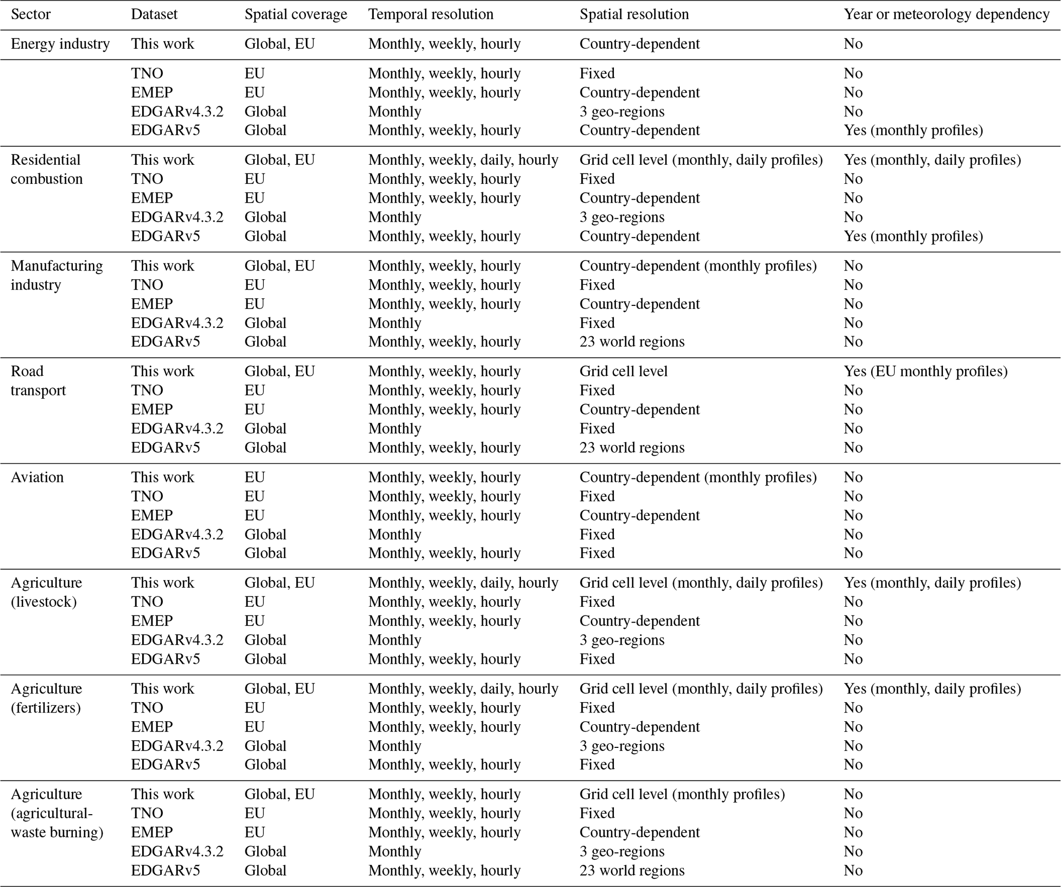
This work presents the Copernicus Atmosphere Monitoring Service TEMPOral profiles (CAMS-TEMPO), a new dataset of global and European emission temporal profiles for atmospheric chemistry modelling. The development of CAMPS-TEMPO comes from the need to overcome the aforementioned limitations of current profiles (i.e. use of an outdated source of information and neglection of the temporal variation of emissions across species and countries or regions) and to improve the representation of the emission temporal variations, which was defined as a priority task within the Copernicus global and regional emissions service (CAMS_81) directly supporting the CAMS production chains (https://atmosphere.copernicus.eu/, last access: February 2021). Multiple socio-economic, statistical and meteorological data were collected and processed to create the profiles. The CAMS-TEMPO dataset includes monthly, weekly, daily and hourly temporal profiles for the priority air pollutants (NOx; SOx; NMVOC, non-methane volatile organic compound; NH3; CO; PM10; and PM2.5) and the greenhouse gases (CO2 and CH4) and each of the following anthropogenic source categories: energy industry, residential combustion, manufacturing industry, transport (road traffic and air traffic in airports) and agriculture. Depending on the sector and temporal resolution, the profiles are either fixed (spatially constant) or vary spatially by country or region and can be pollutant-dependent and/or year-dependent. The CAMS-TEMPO profiles introduce multiple novel aspects when compared to the current profiles used for air quality modelling, including (i) pollutant dependency, (ii) spatial variability and (iii) meteorological influence. Table 1 summarizes and compares the main characteristics of the CAMS-TEMPO profiles with the ones reported in other datasets including TNO (Denier van det Gon et al., 2011), EMEP (Simpson et al., 2012), EDGARv4.3.2 (Janssens-Maenhout et al., 2019) and EDGARv5 (Crippa et al., 2020) regarding spatial coverage, temporal and spatial resolution, and year or meteorology dependency.
Table 1Main characteristics of the temporal profiles developed in this work compared to those reported in other datasets including TNO (Denier van det Gon et al., 2011), EMEP (Simpson et al., 2012), EDGARv4.3.2 (Janssens-Maenhout et al., 2019) and EDGARv5 (Crippa et al., 2020) regarding spatial coverage, temporal and spatial resolution, and year or meteorology dependency.
The CAMS-TEMPO profiles were created following the domain descriptions (resolution and geographical area covered) and emission sector classification system defined in the CAMS global anthropogenic inventory (CAMS-GLOB-ANT) and CAMS regional inventory for air pollutants and greenhouse gases (CAMS-REG_AP/GHG), also developed under CAMS_81 (Granier et al., 2019).
The CAMS-GLOB-ANT dataset (Elguindi et al., 2020a) is a global emission inventory developed for the years 2000–2020 at a spatial resolution of 0.1 × 0.1∘ in support of the CAMS global simulations. The data are based on the EDGARv4.3.2 annual emissions developed by the European Commission Joint Research Centre (JRC, Crippa et al., 2018) for the years 2000–2012. After 2012, the emissions are extrapolated to the current year using linear trend fits to the years 2011–2014 from the CEDS (Community Emissions Data System) global inventory (Hoesly et al., 2018), which provides historical emissions for the Sixth Assessment Report (AR6) of the IPCC (Intergovernmental Panel on Climate Change). Emissions are provided for the main pollutants and greenhouse gases, together with a speciation of NMVOCs based on Huang et al. (2017). A comparison of CAMS-GLOB-ANT emissions to the other inventories is presented in Elguindi et al. (2020b).
The CAMS regional emissions are being prepared for air pollutants and greenhouse gases (CAMS-REG_AP/GHG), in support of the CAMS regional production systems and policy tools. The inventory is built up largely using the official reported emission data from individual countries in Europe for each source category, which has the main advantage that it takes into account country-specific information on technologies, practices and associated emissions. Where these data were either unavailable or not fit for purpose, these were replaced with other estimates. Then, a consistent spatial distribution is applied across Europe at a resolution of 0.1 × 0.05∘ by means of using proxies for each source category of emissions. These proxies include among others point source emissions from E-PRTR (European Pollutant Release and Transfer Register), road networks, land use and population density information. Shipping emissions are taken from the STEAM (Ship Traffic Emission Assessment Model) model (Johansson et al., 2017). By also providing speciation profiles for PM (particulate matter) and VOCs (volatile organic compounds), as well as default height profiles, the dataset is fit for purpose for air quality modelling at the European scale. Different versions of the CAMS regional emissions are available, with the latest version (v4.2) covering the years 2000–2017 having been produced in early 2020. The methodology used for an earlier version of this inventory is available (Kuenen et al., 2014), and a new publication is currently in preparation for the latest version (Kuenen et al., 2021).
The paper is organized as follows. Section 2 describes, for each sector, the approaches and sources of information used to develop the CAMS-TEMPO profiles. Section 3 discusses the obtained temporal profiles and compares them to currently available datasets. Section 4 provides a description of the data availability, and finally Sect. 5 presents the main conclusions of this work.
2.1 Overview
The following subsections describe the input data and methodologies used to compute the CAMS-TEMPO emission temporal profiles for each targeted sector: (i) energy industry (Sect. 2.2), (ii) residential and commercial combustion (Sect. 2.3), (iii) manufacturing industry (Sect. 2.4), (iv) road transport (Sect. 2.5), (v) aviation (Sect. 2.6), and (vi) agriculture (Sect. 2.7).
The CAMS-TEMPO dataset consists of a collection of global and regional temporal factors that follow the domain description and sector classification reported by the CAMS-GLOB-ANT and CAMS-REG_AP/GHG emission inventories. In order to better distinguish between the two sets of profiles, we refer to them as CAMS-GLOB-TEMPO (https://doi.org/10.24380/ks45-9147, Guevara et al., 2020a, global temporal profiles associated with the CAMS-GLOB-ANT inventory) and CAMS-REG-TEMPO (https://doi.org/10.24380/1cx4-zy68, Guevara et al., 2020b, regional European temporal profiles associated with the CAMS-REG_AP/GHG inventory). Depending on the pollutant source and temporal resolution (i.e. monthly, weekly, daily and hourly), the resulting profiles are reported as spatially invariant (i.e. a unique set of temporal weights for the entire domain, Tables A1 to A4 in Appendix A of this work) or gridded values (i.e. temporal weights vary per grid cell). Similarly, depending on the characteristics of the input data used and approaches to compute the profiles, these can be year-dependent and/or pollutant-dependent. The spatial resolution of the gridded profiles is 0.1 × 0.1∘ for CAMS-GLOB-TEMPO and 0.1 × 0.05∘ for CAMS-REG-TEMPO. In the case of CAMS-REG-TEMPO, the domain covered by the dataset is 30∘ W–60∘ E and 30–72∘ N.
Tables 2 and 3 summarize the characteristics of each temporal profile included in the CAMS-GLOB-TEMPO and CAMS-REG-TEMPO datasets, respectively. The sector classification for each case corresponds to those used in CAMS-GLOB-ANT and CAMS-REG_AP/GHG. The specificity of the computed profiles depends upon the degree of sectoral disaggregation used in the original CAMS inventories. For example, the CAMS-GLOB-ANT dataset reports emissions from power and heat plants and refineries under the same sector (“ene”, see Table 2), and therefore a common set of temporal profiles had to be assumed for the two types of facilities. In contrast, the CAMS-REG_AP/GHG inventory reports power and heat plants under the GNFR_A (Gridding Nomenclature for Reporting) category (public power) and refineries under sector GNFR_B (industry), together with all manufacturing industries (Table 3). All the assumptions made regarding this topic are clearly stated in each subsection.
Table 2Main characteristics of the CAMS global temporal profiles (CAMS-GLOB-TEMPO) reported by sector and temporal resolution (monthly, daily, weekly and hourly). The text between brackets gives information on the spatial resolution and pollutant and year dependency of each profile. Gridded indicates that the profile varies per grid cell within a country; per country indicates that the profile varies only per country; fixed indicates that the profile is spatially invariant; year-independent indicates that the profiles does not vary per year; year-dependent indicates that the profile varies per year; pollutant-independent indicates that the same profile is proposed for all pollutants (NOx, SOx, NMVOC, NH3, CO, PM10, PM2.5, CO2 and CH4); pollutant-dependent indicates that the profile varies per pollutant; per day type indicates that the profile varies as a function of the day (weekday, Saturday and Sunday). The symbol “–” denotes that no profile is proposed.

a Leap or non-leap years. b Same profiles as the ones reported by the TNO dataset (Denier van der Gon et al., 2011).
Table 3Main characteristics of the CAMS regional temporal profiles (CAMS-REG-TEMPO) reported by sector and temporal resolution (monthly, daily, weekly and hourly). The text between brackets gives information on the spatial resolution and pollutant and year dependency of each profile. Gridded indicates that the profile varies per grid cell within a country; per country indicates that the profile varies only per country; fixed indicates that the profile is spatially invariant; year-independent indicates that the profiles does not vary per year; year-dependent indicates that the profile varies per year; pollutant-independent indicates that the same profile is proposed for all pollutants (NOx, SOx, NMVOC, NH3, CO, PM10, PM2.5, CO2 and CH4); pollutant-dependent indicates that the profile varies per pollutant; per day type indicates that the profile varies as a function of the day (weekday, Saturday and Sunday). The symbol “–” denotes that no profile is proposed.
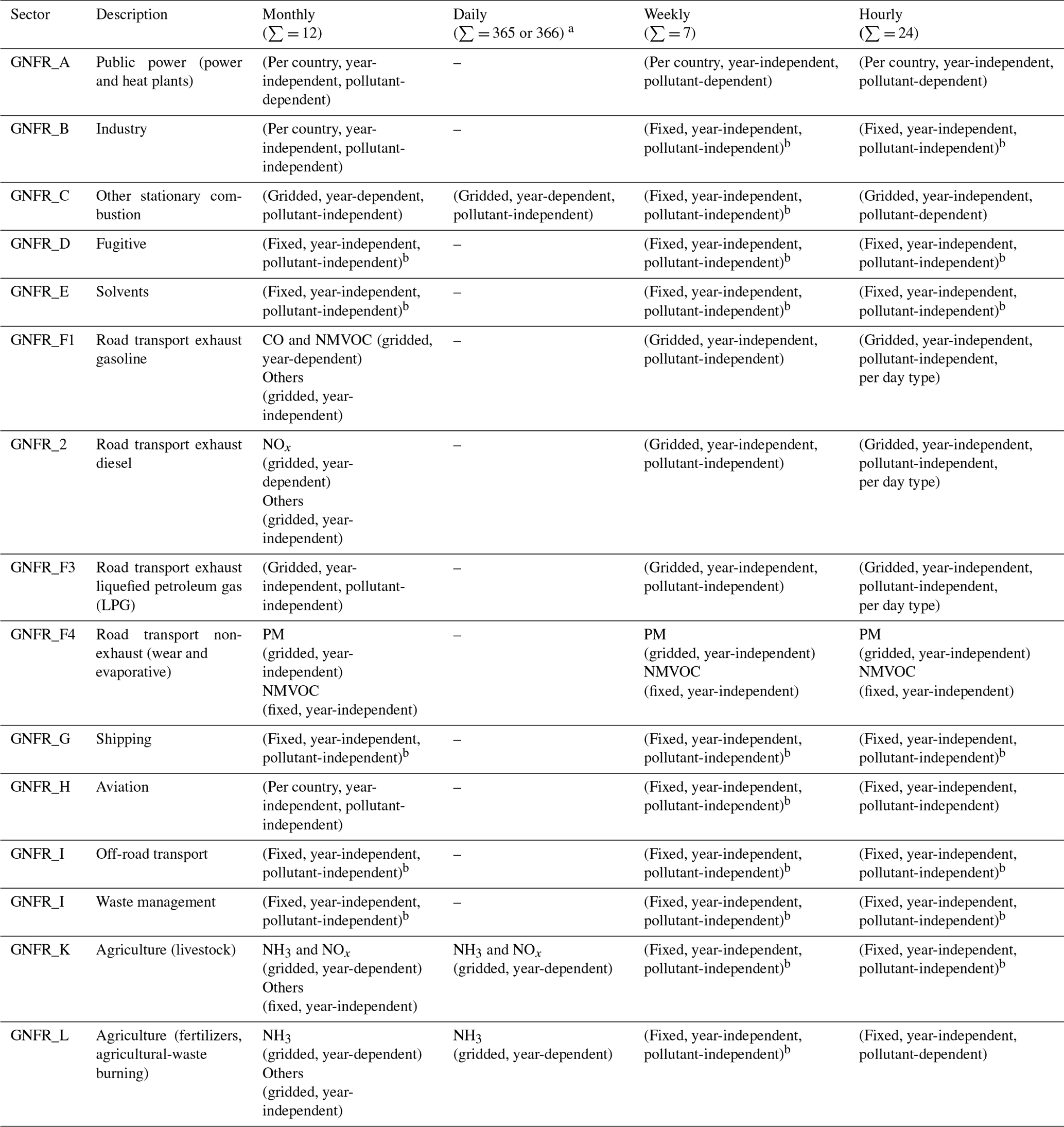
a Leap or non-leap years. b Same profiles as the ones reported by the TNO dataset (Denier van der Gon et al., 2011).
For both CAMS-GLOB-TEMPO and CAMS-REG_AP/GHG, the sum of all temporal weight factors is equal to 12 for monthly profiles, 7 for weekly profiles, 365 or 366 (in the case of a leap year) for daily profiles, and 24 for hourly profiles. Note that the hourly temporal profiles in CAMS-TEMPO are provided in local standard time (LST). The conversion from LST to coordinated universal time (UTC) as a function of time zones is a process that needs to be performed by the final user. Time zone adjustments is a process typically performed by the emission processing systems or tools designed to adapt emission data to the air quality modelling requirements (e.g. Guevara et al., 2019).
2.2 Energy industry
The temporal profiles computed for the energy industry are reported under the ene sector in CAMS-GLOB-TEMPO and the GNFR_A category in CAMS-REG-TEMPO. The temporal variability of emissions from this sector was estimated from electricity production statistics under the assumption that it largely depends upon the combustion of fossil fuels in power and heat plants. This approximation is consistent with the definition of the GNFR_A sector in the CAMS-REG_AP/GHG dataset. The representativeness of the computed profiles is likely lower in CAMS-GLOB_TEMPO because the ene sector also includes other facilities such as refineries.
As shown in Tables 2 and 3, the profiles reported for this sector include pollutant- and country-dependent monthly, weekly and hourly factors. The electricity production dataset compiled to derive profiles for this sector were as follows:
-
The ENTSO-E Transparency Platform. The European Network of Transmission System Operators for Electricity (ENTSO-E; Hirth et al., 2018; ENTSO-E, 2018) centralizes the collection and publication of the electricity generation per production type for each European member state. The information published by the Transparency Platform is collected from data providers such as transmission system operators (TSOs), power exchanges or other qualified third parties. The information collected included production data (in MW) per country and fuel type (i.e. lignite, hard coal, natural gas, oil and biomass) at monthly (years 2010–2014) and hourly (years 2015–2017) levels.
-
The US EPA emission modelling platform. The Environmental Protection Agency (EPA; US EPA, 2019a) maintains an emission modelling platform that includes processed and clean hourly emission data derived from a continuous emission monitoring system (CEMS). The information collected includes hourly NOx, SOx and heat input data for individual power plants in the years 2011 and 2014.
-
The IEA electricity statistics. The International Energy Agency (IEA; IEA, 2021) provides consistent electricity statistics split by generation type (i.e. total fossil fuels, nuclear, hydro, and geothermal or other) and country. The information collected included monthly data for the years 2010 to 2017 for each member country of the Organisation for Economic Co-operation and Development (OECD).
-
The MBS Online. The Monthly Bulletin of Statistics (MBS; MBS, 2018) is a database of the United Nations with a focus on national economic and social statistics. It provides monthly data of the total electricity gross production per country. The information collected included data for the year 2015.
Figure 1a illustrates the spatial coverage of the compiled dataset by source of information (i.e. ENTSO-E, US EPA, IEA and MBS). Overall, main emission producers (e.g. China, India, Europe and North America) are covered, while most of the countries with no information available are located in South America and Africa. For those countries with no data, the TNO profiles reported under the energy sector (Denier van der Gon et al., 2011) are used.
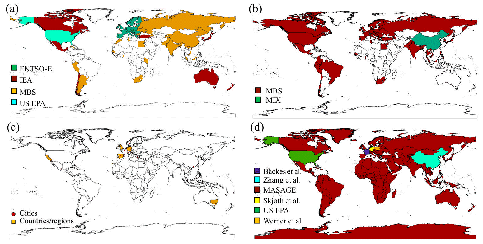
Figure 1Representation of the spatial coverage of the datasets used to derive temporal profiles for the energy industry (a), the manufacturing industry (b), road transport (c) and agriculture (use of fertilizers) (d). For the energy industry, the legend indicates the different sources of information used: the European Network of Transmission System Operators for Electricity (ENTSO-E), the United States Environmental Protection Agency (US EPA), the International Energy Agency (IEA) and the Monthly Bulletin of Statistics (MBS). For the manufacturing industry, the legend indicates the sources of information used: the MBS and the MIX inventory (mosaic Asian anthropogenic emission inventory, Li et al., 2017). For agriculture, sources of information are also highlighted: Backes et al. (2016), Zhang et al. (2018), the MASAGE_NH3 (Magnitude And Seasonality of Agricultural Emissions model for NH3) inventory (Paulot et al., 2014), US EPA (2019b), Skjøth et al. (2011) and Werner et al. (2015). Administrative boundaries are derived from GADM (2020).
The compiled data were first analysed to assess whether interannual variability is important for this sector. Seasonal cycles were computed for different years (2010–2017) and countries using the IEA statistics. In the majority of the countries analysed, the monthly profiles were found to be consistent through the different years and to present small interannual variations (Fig. S1 in the Supplement). Although some studies have pointed out a temperature dependence of the monthly electricity generation in power plants (Thiruchittampalam, 2014), we neglected it at present. Consequently, we assume the monthly temporal profiles for this sector to be the average over all the available years of data.
2.2.1 Monthly profiles
For European countries, monthly profiles were derived using the ENTSO-E dataset. The analysis of the data showed that the seasonality of electricity production varies significantly by fuel type (Fig. S1). The different use of energy sources (i.e. lignite, hard coal, natural gas, biomass and oil) implies that temporal patterns will also vary from one pollutant to another. For each month, country and pollutant, profiles were calculated following Eq. (1):
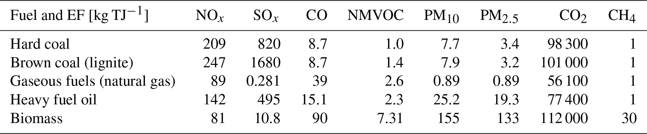
where is the monthly factor for month m, country c and pollutant p; is the is the monthly factor for month m, country c and fuel f; FSc,f is the fuel share factor for country c and fuel f; and EFf,p is the emission factor for fuel f and pollutant p. Fuel share factors were obtained by averaging the ENTSO-E production data for the years 2010 to 2017 per country, and the emission factors were taken from the EMEP/EEA (European Environmental Agency) 2016 emission inventory guidebook for the priority air pollutants (EMEP/EEA, 2016; 1.A.1 “Energy industries”, Tables 3-2, 3-3, 3-4, 3-5 and 3-7) and from the IPCC guidelines (IPCC, 2006; Volume 2: “Energy”, Table 2.2) for GHGs (greenhouse gases) (Table 4). We note that only fuels with shares larger than 10 % were considered. For instance, in the case of Austria, only hard coal (25 %) and natural gas (65 %) were used, and the original shares were normalized so that their sum equalled 100 %. This was done to avoid introducing errors due to residual fuels, which may be related to few (or even just one) power plants.
Table 4Emission factors [kg TJ−1] related to the energy industry per fuel type and pollutant. Values obtained from the EMEP/EEA 2016 emission inventory guidebook for the priority air pollutants (1.A.1 “Energy industries”, Tables 3-2, 3-3, 3-4, 3-5 and 3-7) and from the IPCC guidelines (Volume 2: “Energy”, Table 2.2) for greenhouse gases.
For other countries, monthly factors by pollutant could not be developed, as both the IEA and the MBS datasets do not report electricity production split by fuel type. Hence, monthly factors were derived by averaging the available production data per month and relating them to the total production in the year. For the US, NOx and SOx monthly profiles were derived from the corresponding hourly measured emissions reported by the EPA's CEMS data. Measurements from all individual plants were averaged at the monthly level and then normalized to sum 12. The seasonality for the other pollutants (i.e. NMVOC, NH3, CO, PM10, PM2.5, CO2 and CH4) was linked to the measured heat input, following Stella (2005).
2.2.2 Weekly profiles
Weekly profiles were developed for Europe using the hourly electricity production data reported by ENTSO-E. As in the case of the monthly profiles, weekly scale factors were found to significantly vary according to the type of fuel (Fig. S1). These results are in line with the conclusions of Adolph (1997), which identified three generic weekly profiles – base, medium and peak load – as a function of the type of power plant. Pollutant-related weekly profiles were developed following the same methodology applied for obtaining the monthly weight factors (Eq. 1).
For the US, the CEMS data were used to compute pollutant-dependent profiles following the same procedure as described in Sect. 2.2.1. Measurements from all individual plants were averaged per day of the week and then normalized to sum 7. For countries with no information on daily electricity production data, we used the weekly profile reported in the TNO dataset for the energy sector.
2.2.3 Hourly profiles
Hourly profiles were developed for Europe and the US using the hourly electricity production data reported by ENTSO-E and the measured emissions reported by CEMS, respectively. As previously seen, large differences are observed between fuels. Profiles related to the so-called base peak load power plants (i.e. annual useful life of more than 4000 h) present a rather flat distribution, whereas in other cases the change in energy production between day and night is relatively high (Fig. S1).
Pollutant-related hourly profiles were developed following the same procedure shown in Eq. (1). For countries with no information on hourly electricity production data, we assumed the hourly profile reported in the TNO dataset. Some studies have suggested that the hourly variation of power plant activities may vary according to the season of the year (Thiruchittampalam, 2014). This feature is not considered in the present version of the CAMS-TEMPO profiles and will be addressed in future releases.
2.3 Residential and commercial combustion
The temporal profiles computed for the residential and commercial sector are reported under the res sector in CAMS-GLOB-TEMPO and the GNFR_C category in CAMS-REG-TEMPO. The temporal variability of emissions for this sector is assumed to be dominated by the stationary combustion of fossil fuels in households and commercial and public service buildings. These categories are also assumed to be the main contributors to the total emissions reported by CAMS-GLOB-ANT and CAMS-REG_AP/GHG. Other combustion installations activities included under this sector (i.e. plants in agriculture, forestry and aquaculture and other stationary facilities including military) are assumed to follow the same temporal profile.
The temporal weight factors developed for this sector include monthly, daily and hourly profiles. The monthly and daily profiles depend upon year and region and were derived using meteorological parametrizations (Sect. 2.3.1). The hourly profiles depend upon pollutant and region (Sect. 2.3.2).
2.3.1 Monthly and daily profiles
Gridded daily temporal profiles were derived according to the heating-degree-day (HDD) concept, which is an indicator used as a proxy variable to reflect the daily energy demand for heating a building (Quayle and Diaz, 1980). This method has been proven to be successful in previous emission modelling work (e.g. Mues et al., 2014; Terrenoire et al., 2015).
The heating-degree-day factor (HDD(x,d)) for grid cell x and day d is defined relative to a threshold temperature (Tb), above which a building needs no heating (i.e. heating appliances will be switched off), following Eq. (2):
where T2 m(x,d) is the daily mean 2 m outdoor temperature for grid cell x and day d [∘C]. This information was obtained from the ERA5 reanalysis dataset for the period 2010–2017 (C3S, 2017). As shown in Eq. (2), HDD(x,d) increases with the difference between the threshold and actual outdoor temperatures. A minimum value of 1 is assumed instead of 0 to avoid numerical problems when used in Eq. (3).
A challenge when using this method is to set the threshold or comfort temperature (Tb). The choice of Tb depends on local climate and building characteristics, among others. When dealing with an extended area like Europe or even the whole world, it is difficult to choose a unique Tb. This value is usually set to 18 ∘C (e.g. Mues et al., 2014), 15.5 ∘C (e.g. Spinoni et al., 2015) or even 15 ∘C (e.g. Stohl et al., 2013). Following the work by Spinoni et al. (2015), which developed gridded European degree-day climatologies, we assumed that Tb=15.5 ∘C, a value also suggested by the UK Met Office. A first guess of the daily temporal factor (FD(x,d)) for grid cell x and day d is (Eq. 3)
where is the yearly average of the heating-degree-day factor per grid cell x (Eq. 4),
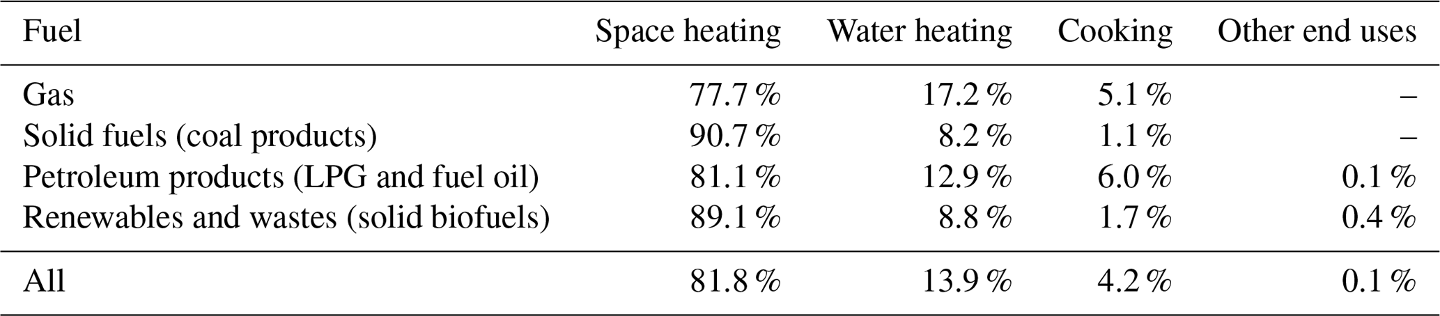
where N=365 or 366 d (leap or non-leap year). Considering that residential combustion processes are related not only to space heating but also to other activities that remain constant throughout the year such as water heating or cooking, a second term is introduced to Eq. (5) by means of a constant offset (f) (Eq. 5):
where f=0.2 based on the European household energy statistics reported by Eurostat (2018) (Table 5). As observed, this share may vary depending on fuel. In the case of biofuels or coal products, which dominate the contribution to total PM emissions, space heating represents 89.1 % of the residential combustion processes (f∼ 0.1), whereas in the case of natural gas, which is the main contributor to NOx, the share is 77.7 % (f∼ 0.2). Significant differences between countries are also observed for specific fuels. For instance, in Norway 100 % of solid fuels are used for space heating (f∼ 0), whereas in Greece this share is only 65 % (f∼ 0.35), with the remainder being attributed to water heating (27 %) and cooking (8 %) (Eurostat, 2018). More significant differences can be found in developing regions (e.g. Tibetan Plateau), where the share of solid biofuels used for cooking can go up to 80 %. Despite these variations, a generic value of f=0.2 is assumed for all regions. To illustrate how current assumptions may impact the derived profiles in non-European regions, we computed daily factors for the residential sector over India and China for 2015 using a range of f (0, 0.2 and 0.5) and Tb (15.5 and 18 ∘C) values (Fig. S2). We selected these two countries, as they produce a large share of the global residential emissions (Hoesly et al., 2018). Differences between the daily factors of up to 55 % were found during wintertime when comparing the results computed with f=0.0 and 0.5, indicating that daily factors are sensitive to these parameters. The investigation and proposal of different f values (as well as different Tb values) for different regions of the world will be addressed in future work.
Gridded daily temporal profiles were developed for 8 years (2010 to 2017). A climatological daily profile based on the average of each day over all the available years was also produced. Monthly gridded factors were derived from the daily profiles for all the years available. We interpolated the estimated gridded daily factors from the ERA5 working domain (approx. 0.3×0.3∘) onto the CAMS-GLOB-ANT (0.1 × 0.1∘) and CAMS-REG_AP/GHG (0.05×0.1∘) grids, applying a nearest-neighbour approach.
2.3.2 Hourly profiles
The hourly distribution of residential and commercial combustion activities has typically been described following the profile A presented in Fig. 2a, used in both EMEP and TNO datasets. This hourly distribution presents one peak in the morning and another one in the afternoon, when energy consumption is supposedly higher due to increased space heating or cooking activities. We evaluated this profile with real-world measurements of natural gas consumption for residential houses in the UK (Retrofit for the Future project, https://www.ukgbc.org/ukgbc-work/retrofit-for-the-future-innovate-uk/, last access: February 2021) and the US state of Texas (Data Port – Pecan Street dataset, https://dataport.cloud/, last access: February 2021) and a house in Canada (Makonin et al., 2016). The measurements show the two peaks in all the profiles, although their occurrence and intensity vary due to the specific energy consumption behaviour of each house (Fig. S2). This comparison suggests that profile A is representative of emissions related to natural gas combustion.
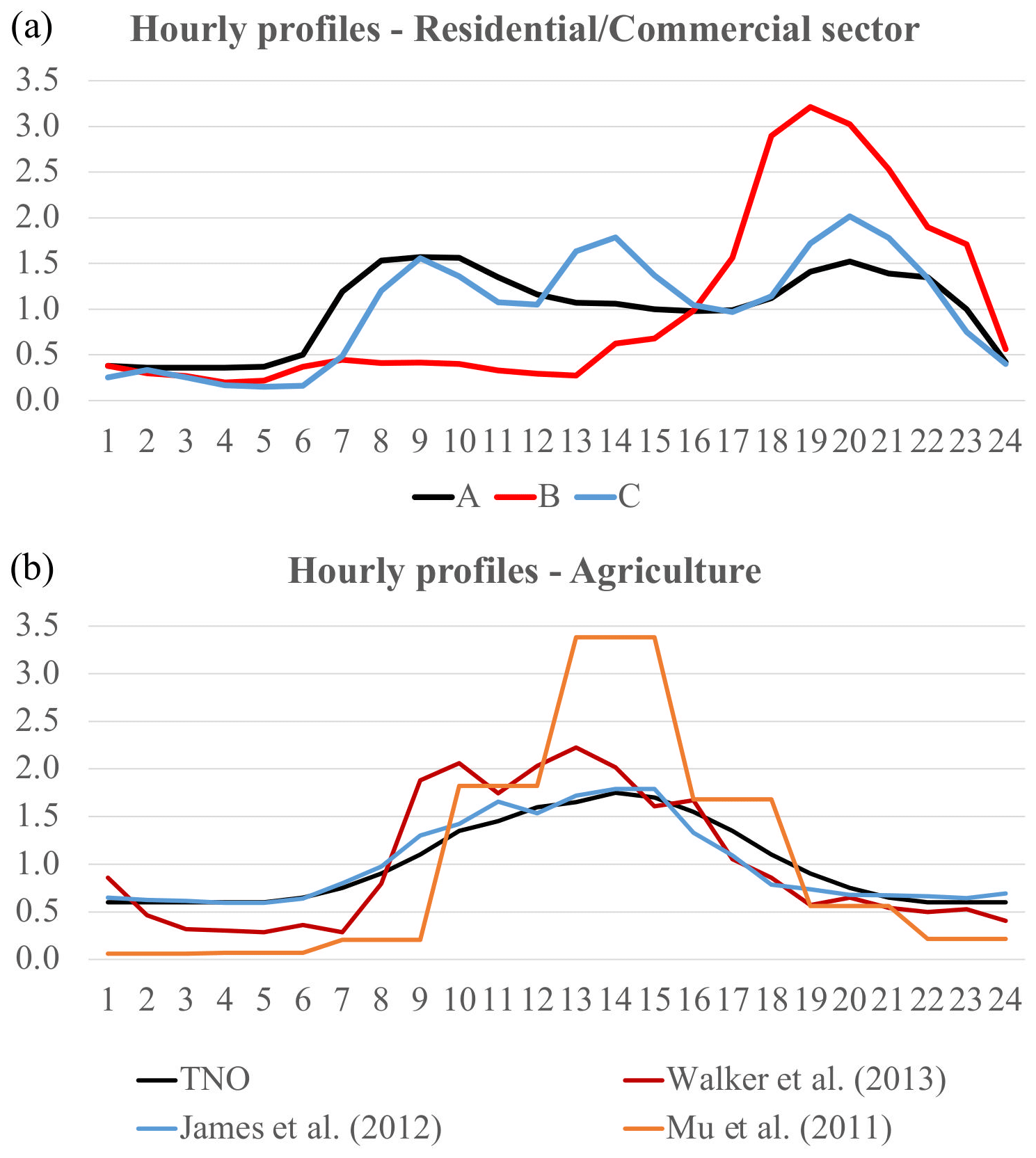
Figure 2(a) Proposed hourly temporal profiles for the residential and commercial combustion sector where profile A refers to NOx, SOx and CH4 emissions in urban and rural areas of developed and developing countries; profile B refers to PM10, PM2.5, CO, CO2, NMVOC and NH3 in urban and rural areas of developed countries; and profile C refers to all pollutants in rural areas of developing countries. (b) Comparison between the hourly temporal profile proposed by TNO for agricultural emissions (Denier van der Gon et al., 2011) and the three measurement-based temporal profiles reported by Walker et al. (2013) derived from NH3 flux measurements performed in a fertilized corn canopy in North Carolina, James et al. (2012) based on direct NH3 measurements performed in a mechanically ventilated swine barn and Mu et al. (2011) derived from active fire satellite observations.
We created a second hourly profile (Fig. 2a, profile B) linked to the combustion of residential wood for space-heating purposes using as a basis information derived from citizen interviews performed in Norway and Finland (Finstad et al., 2004 and Gröndahl et al., 2010) as well as from long-term measurements of the wood-burning fraction of black carbon in Athens (Athanasopoulou et al., 2017). As shown in Fig. 2a, the resulting profile B presents an intense peak during the evening hours, but not during the morning, in contrast to profile A. It is actually a common practice in developed countries to use fireplaces and other types of wood-burning appliances mainly in the evening.
As reported by the World Health Organization (WHO), most developing countries use wood not only for heating space purposes but also for cooking activities (Bonjour et al., 2013). We created a third profile that represents these activities (Fig. 2a, profile C) based on information derived from continuous indoor PM2.5 measurements performed in households in the eastern Tibetan Plateau (Carter et al., 2016). The profile is influenced by heating and cooking practices and therefore presents three peaks that correspond to typical morning, midday and evening mealtimes.
The results summarized in Fig. 2a indicate that the hourly behaviour of residential combustion emissions varies according not only to the fuel type but also to the type of end use (i.e. space heating or cooking). Both CAMS-GLOB-ANT and CAMS-REG_AP/GHG report total residential and commercial emission as a unique sector, without discriminating by type of fuel or end use. Therefore, several decisions were made in order to assign the three proposed profiles to different pollutants and regions:
-
profile A: NOx, SOx and CH4 emissions in urban and rural areas of developed and developing countries;
-
profile B: PM10, PM2.5, CO, CO2, NMVOC and NH3 in urban and rural areas of developed countries; and
-
profile C: all pollutants in rural areas of developing countries.
The assumptions made behind this assignment are the following:
-
Natural gas and diesel heating combustion is the main contributor to total NOx, SOx and CH4 emissions.
-
Wood combustion is the main contributor to total PM10, PM2.5, CO, CO2, NMVOC and NH3 emissions.
-
In the urban and rural areas of developed countries wood is mainly used for heating purposes.
-
In the urban areas of developing countries wood is mainly used for heating purposes.
-
In the rural areas of developing countries all fuels are used both for heating and/or cooking purposes (i.e. the two activities occur at the same time).
The list of developing countries was obtained from the World Bank country classifications (World Bank, 2014). The discrimination of human settlements between urban and rural areas was derived from the Global Human Settlement Layer (GHSL) project (Florczyk et al., 2019; Pesaresi et al., 2019). The GHSL provides a global classification of human settlements on the basis of the built-up settlement and population density at a resolution of 1 km × 1 km corresponding to four epochs (2015, 2000, 1990 and 1975). The 2015 epoch was selected, and the original raster was remapped onto the CAMS-GLOB-ANT (0.1 × 0.1∘) and CAMS-REG_AP/GHG (0.1 × 0.05∘) grids.
2.4 Manufacturing industry
The temporal variability of industrial emissions is reported under the sectors indu (CAMS-GLOB-TEMPO) and GNFR_B (CAMS-REG-TEMPO). Both in the CAMS-GLOB-ANT and the CAMS-REG_AP/GHG inventories, all industrial manufacturing emissions are reported under these single categories. Hence, the same temporal pattern has to be assumed for all types of facilities (e.g. cement plants, iron and steel plants, and food and beverage). For this sector, only country-dependent monthly profiles were developed due to the lack of more detailed data.
2.4.1 Monthly profiles
Country-specific monthly profiles were estimated using the Industrial Production Index (IPI), which measures the monthly evolution of the productive activity of different industrial branches, including manufacturing activities. The IPI as a monthly surrogate for industrial emissions has been used in previous studies (e.g. Pham et al., 2008; Markakis et al., 2010).
The IPI data were obtained from the MBS database (MBS, 2018), which provides monthly information per country and general industrial branch (i.e. mining, manufacturing, electricity, gas and steam, and water supply) for the year 2015. The manufacturing branch, which includes several divisions such as iron and steel industries, chemical industries, and food and beverage products, was used to derive country-specific monthly profiles. Figure 1b shows the spatial coverage of the compiled dataset. As in the case of the energy industry sector (Fig. 1a), the lack of information mostly affects Africa and South America. For those countries without available information, the monthly profile reported in the TNO dataset under the industry sector was used (Denier van der Gon et al., 2011). In the case of China, the monthly profile reported in the MIX inventory under the industry sector was used (Li et al., 2017).
The time profiles are based on IPI information from 2015 and are assumed to be representative for other years. Our assumption is supported by the low interannual variability observed in the IPI values collected from different national statistical offices including Italy (ISTAT, 2018), Norway (SSB, 2018), Spain (INE, 2018) and the UK (ONS, 2018) (Fig. S3). Another implicit assumption made is that the constructed monthly profiles can be equally applied to all the different industrial activities reported under the ind and GNFR_B sectors. The national IPI values collected for Italy and the US (Board, 2020) were used to compare the seasonality of individual industrial divisions to the general manufacturing IPI monthly profile. For both countries, as well as up to a certain extent, it was found that all the industrial divisions (except food and beverages and the petrochemical industry in the case of Italy) follow the seasonality of the general manufacturing profile (Fig. S4), which allows for concluding that the assumption made is reasonable. A similar result is reported for Thailand in Pham et al. (2008).
Table 5Share of final energy consumption in the residential sector by fuel and type of end use in Europe (Eurostat, 2018).
2.4.2 Weekly and hourly profiles
Due to the lack of country-specific data, the fixed weekly and hourly temporal profiles provided in the TNO dataset for industry sector are used. The weekly profile assumes a flat distribution during the working days and a slight decrease during weekends (Table A2). On the other hand, the hourly profile includes an increase of the activity during the central hours of the day (Tables A3 and A4).
2.5 Road transport
Temporal profiles for road transport emissions are reported under the tro sector in CAMS-GLOB-TEMPO and the GNFR_F1 (exhaust gasoline), GNFR_F2 (exhaust diesel), GNFR_F3 (exhaust LPG gas) and GNFR_F4 (non-exhaust) categories in CAMS-REG-TEMPO. The fact that CAMS-REG_AP/GHG traffic-related emissions are classified into four different categories (discriminated by fuel and type of process) allows for considering specific temporal features associated with each one of them, including temperature dependence of CO and NMVOC gasoline exhaust emissions (GNFR_F1), of NOx diesel exhaust emissions (GNFR_F2) and of NMVOC non-exhaust emissions (GNFR_F4). On the other hand, in CAMS-GLOB-ANT all traffic emissions are reported under a single sector, and subsequently the approach used for the development of the temporal profiles is more simplistic.
The temporal weight factors developed for this sector include monthly, weekly and hourly profiles. As summarized in Table 2, the CAMS-GLOB-TEMPO monthly and weekly profiles constructed for this sector are region-dependent, whereas the hourly profiles vary per region and day of the week (i.e. weekday, Saturday and Sunday). In the case of CAMS-REG-TEMPO, the constructed profiles can vary by region, pollutant, day of the week and/or year, as a function of the source sector and temporal resolution (Table 3). Depending on the dataset and sector category, temporal emission variability is assumed to be either exclusively driven by the traffic activity data (e.g. CAMS-GLOB-TEMP, all cases) or by a combination of traffic activity data and changes in ambient temperature (i.e. CAMS-REG-TEMP, CO and NMVOC GNFR_F1, NOx GNFR_F2, and NMVOC GNFR_F3). For the first case, temporal profiles were developed using traffic count data compiled from multiple sources of information (Sect. 2.5.1). As listed in Table 6, the information was obtained from local and national open-data portals, publications or through personal communications. The spatial coverage of the compiled dataset is illustrated in Fig. 1c. For the second group of profiles, the temporal variability of traffic activity was combined with meteorological parametrizations available in the literature (Sect. 2.5.2).
Table 6List of traffic activity datasets and corresponding sources of information compiled.
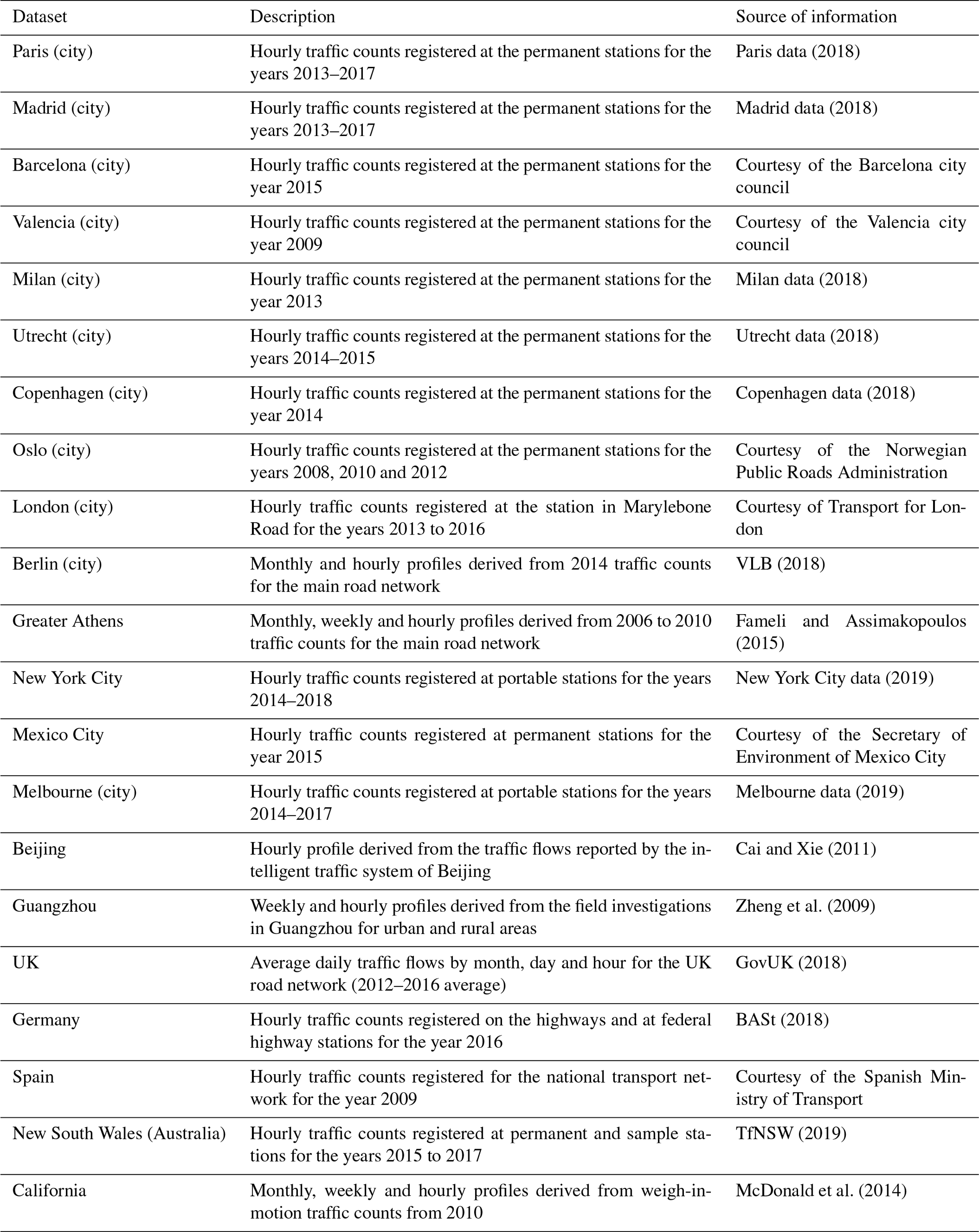
Considering that for each traffic count dataset the reference years are different (Table 6), we analysed the data in view of differences in the resulting profiles as a function of the year. We took the Paris city traffic data as an example, since it covers a wide range of years (2013 to 2017). For each year, monthly, weekly and hourly (i.e. Wednesday and Saturday) profiles were constructed (Fig. S5). The results suggest that temporal patterns in vehicle activity do not change much over long timescales. Consequently and following the assumptions made for the energy and manufacturing industry sectors, we assumed that the interannual variability can be negligible. Hence, all profiles developed only as a function of traffic count data were constructed by averaging the values (per month, day of the week or hour of the day) over all the available years.
Some of the compiled datasets (e.g. Germany and California) report the traffic counts classified by vehicle type (i.e. light-duty vehicles, LDVs, and heavy-duty vehicles, HDVs). The monthly, weekly and hourly profiles as a function of the vehicle type showed significant differences, especially for weekly and hourly profiles (Fig. S6). HDV traffic presents a larger decrease on the weekend than LDV traffic. Moreover, the hourly LDV profile exhibits two distinct (morning and evening) commuter-related peaks, whereas HDV shows a single midday peak. These results highlight the importance of applying separate temporal profiles to characterize traffic and associated emissions for LDVs and HDVs. However, in the present work this disaggregation was not considered, since both the CAMS-GLOB-ANT and CAMS-REG_AP/GHG inventories report LDV- and HDV-related emissions under the same pollutant sector. When only vehicle-type temporal profiles were available (i.e. California), the information reported for LDVs is used, as this type of vehicle dominates the temporal distribution of total traffic flow.
2.5.1 Meteorology-independent monthly profiles
A comparison between monthly variation in traffic patterns at urban and rural locations (i.e. urban streets and highways) was performed for selected countries or regions including California, Germany, Spain and the UK. For the UK and California, the original traffic statistics were already discriminated by type of location. For the German and Spanish datasets, each traffic station was classified as urban or rural considering its geographical location and the GHSL human settlement classification dataset (Sect. 2.3.2). As shown in Fig. 3, while there is little seasonal variation in German urban locations, rural areas tend to exhibit a stronger seasonality, with a peak occurring during summertime, presumably due to increased recreational and vacation-related driving. The results derived from California, Spain and the UK are consistent with these patterns (Fig. S7).
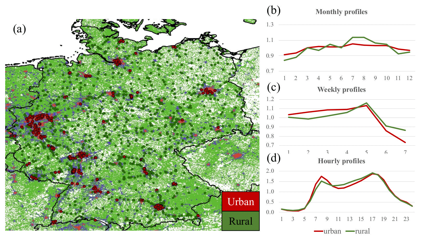
Figure 3Map representing urban and rural human settlements in Germany as reported by the Global Human Settlement Layer (GHSL; Pesaresi et al., 2019) and the location of urban and rural German traffic count stations (a) and monthly, weekly and hourly temporal profiles derived from averaging the original traffic counts (BASt, 2018) by the type of station (b, c, d). Administrative boundaries are derived from GADM (2020).
The datasets collected from several cities (i.e. Athens, Barcelona, Berlin, Copenhagen, London, Madrid, Mexico City, Milan, Oslo and Paris) were also used to construct monthly profiles (Fig. 4a). For comparison purposes, the TNO road transport profile is also included (Denier van der Gon et al., 2011). The three southern European cities (i.e. Athens, Madrid and Milan) together with Paris present a similar pattern, with a significant decrease of the activity during the month of August due to the summer holidays. Similarly, northern European cities (i.e. Copenhagen and Oslo) also present a decrease in summer but of a lower intensity and during July. On the other hand, the seasonality observed in London, Berlin and Mexico City is rather flat and closer to the TNO profile.
Results in Figs. 3b and 4a showed that (i) monthly variations can significantly differ among countries and (ii) within a country, traffic regimes show differences according to the location (urban or rural). Considering all of the above, country- and region-specific (urban or rural) monthly profiles were constructed based on the traffic information compiled. For countries without any available temporal factors, assumptions were made considering geographical proximity. For instance, the urban profile for Scandinavian countries without data (i.e. Finland, Sweden and Iceland) was constructed by averaging the profiles of Oslo and Copenhagen. On the other hand, the rural profile constructed for Spain was assigned to other southern European countries (i.e. Italy, Greece, Malta, Croatia, Bosnia and Herzegovina, Montenegro, Albania, Slovenia, Cyprus, and Portugal). Similarly, the seasonality in Canada was assumed to be equal to the one observed in the US. For all the countries not listed in the table, the urban and rural profiles developed for Germany were assumed. This approach may be further improved as more traffic count data become available. In the case of China and India, profiles were derived from the MIX emission inventory (Li et al., 2017).
Two main assumptions underlie these profiles. First, the differences among cities within a country are assumed to be small, and therefore we use a unique urban profile therein. The second hypothesis was to assume that all the streets and highways located in urban and rural areas present the same seasonality. While this is a reasonable assumption overall, individual traffic count stations can show particular features. For instance, on certain highways near city entrances or crossing urban areas, traffic intensity shows a flat distribution without the typical summer anomalies. This level of detail, which would require a specific temporal profile per road segment, is out of the scope of this dataset but may be explored in future work.
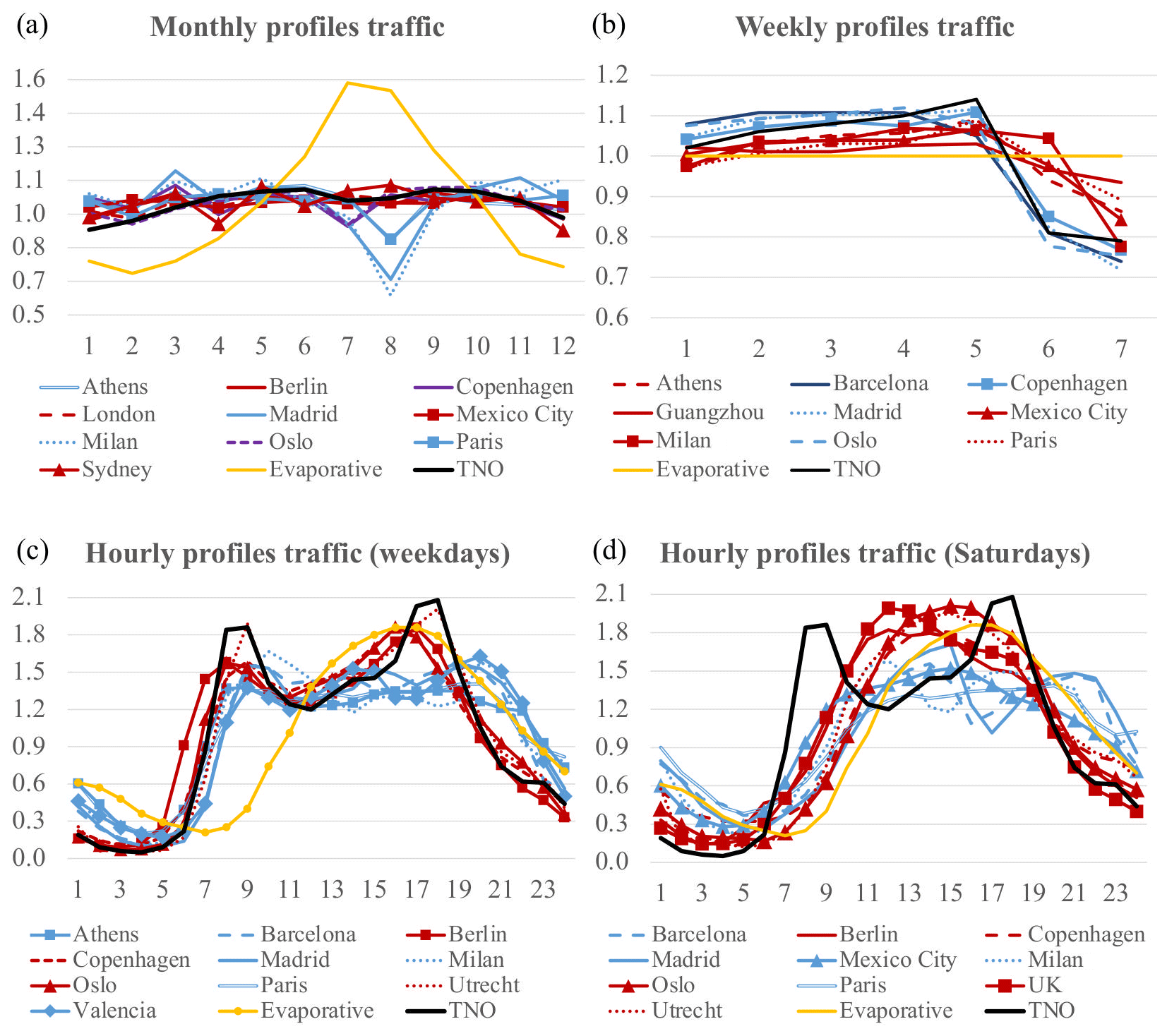
Figure 4Monthly (a), weekly (b) and hourly (c, for weekdays, d for Saturdays) temporal profiles derived from measured traffic counts in selected cities (see Table 6 for references). The profile reported by the TNO dataset is plotted for comparison purposes (Denier van der Gon et al., 2011). The monthly, weekly and hourly profiles proposed for the gasoline evaporative emissions (Evaporative, yellow line) is also shown.
2.5.2 Meteorology-dependent monthly profiles
The seasonality of traffic emissions can be affected by temperature. As shown by Zheng et al. (2014), during winter months vehicles in China produce 19 % more CO and 11 % more NMVOC than in the summer due to the higher contribution of cold-start emissions. This study also showed that the monthly pattern of emissions differs remarkably by latitude, which is explained by the large contribution of cold-start emissions and the relationship between latitude and temperature. More recently, Keller et al. (2017) and Grange et al. (2019) identified strong temperature dependence for diesel vehicle NOx emissions. On the basis of measurements of real-world vehicle emissions, both studies concluded that light-duty diesel NOx emissions are highly dependent on ambient temperature, with low temperatures resulting in higher NOx emissions (up to +80 % for temperatures under 0 ∘C in Euro 5 diesel cars; Keller et al., 2017). Grange et al. (2019) also highlighted the spatial heterogeneity of the so-called “diesel low temperature NOx emission penalty” throughout Europe due to the different climate conditions.
We used available parametrizations (Eqs. 6 to 8) to account for the meteorological drivers of the seasonality of CO and NMVOC gasoline-related emissions (GNFR_F1) (US EPA, 2015) and NOx diesel-related emissions (GNFR_F2) (Keller et al., 2017):
where FMCO(x,m), FMNMVOC(x,m) and are the CO, NMVOC and NOx gridded monthly profiles for grid cell x and month m and T2 m(x,m) is the monthly mean 2 m outdoor temperature for grid cell x and month m. Note that T2 m(x,m) is expressed in ∘F () × ) in Eqs. (6) and (7) and in ∘C in Eq. (8). This difference is due to the fact that the first two expressions are derived from the North American MOtor Vehicle Emission Simulator (MOVES), while the last one is derived from the European Handbook Emission Factors for Road Transport (HBEFA) model. Monthly gridded 2 m temperature was taken from ERA5 for the period 2010–2017 (CS3, 2017). The obtained monthly profiles were normalized so that their total sum equals 12.
The meteorology-dependent monthly profiles were then combined with the meteorology-independent ones (Sect. 2.5.1) so that the resulting seasonality accounts for both temperature influences and traffic activity. For CO, we used a weight factor of 45 % for the temperature-dependent profiles and of 55 % for the traffic activity ones, following the UK National Atmospheric Emissions Inventory (NAEI), which reports road transport annual emissions and distinguishes between cold starts and hot exhaust. Due to the lack of information, we assumed the same share for all countries. Likewise, for NMVOC profiles we assumed a 33 % weight for the temperature-dependent temporal factors (i.e. emissions related to cold starts) and 67 % for the ones derived from traffic counts (i.e. emissions related to hot exhaust). Finally, for NOx we assumed a 50 % and 50 % split, since the “diesel low temperature NOx emission penalty” affects total exhaust diesel emissions (cold starts and hot exhaust).
In addition to the meteorological-dependent profiles described above, we created a specific monthly profile for NMVOC evaporative emissions (GNFR_F4) based on recent results obtained with the High-Elective Resolution Modelling Emission System (HERMESv3) (Guevara et al., 2020c). The HERMESv3 model computes hourly gasoline evaporative emissions from standing cars (diurnal losses) using the “Tier 2” approach reported in the EMEP/EEA emission inventory guidelines 2016. Summer and winter temperature-dependent emission factors are defined for each type of vehicle as a function of the 2 m outdoor temperature obtained from the ERA5 reanalysis. The HERMESv3 model was run over Spain for the year 2016 at a spatial resolution of 4×4 km and a temporal resolution of 1 h. The results aggregated by month and normalized (orange line in Fig. 4a and Table A1) show a strong seasonality, with emissions increasing up to 100 % during summer. We used this profile as a first step that reflects the different dynamics of exhaust and evaporative emissions. Future work may consider developing region-specific profiles for NMVOC evaporative-related emissions.
2.5.3 Weekly profiles
Country- and region-specific (urban or rural) weekly profiles were constructed based on the traffic information summarized in Table 6. In contrast to urban areas, rural traffic activity is lower during weekdays and decrease relatively less during the weekend, especially on Sundays (Figs. 3c and S7). Figure 4b shows how, depending on the location, the intensity of the weekend decrease is relatively higher (e.g. Madrid) or lower (e.g. Mexico City), which is likely due to different sociodemographic patterns. We used the weekly profile provided in the TNO dataset as the urban profile for the countries where local information is not available. Similarly, we used an average profile including data from Germany, Spain and the UK as the rural profile for countries without data. The resulting profiles were assigned equally to all the traffic-related categories of both CAMS-GLOB-TEMPO and CAMS-REG-TEMPO, with the exception of NMVOC gasoline evaporation (GNFR_F4), for which a flat profile is proposed.
2.5.4 Hourly profiles
The analysis of hourly profiles constructed per day of the week for six cities (i.e. Berlin, Madrid, Milan, Oslo, Paris and Utrecht) clearly highlights the need to create hourly profiles per day type (Fig. S9). Weekdays (i.e. Monday to Friday) tend to exhibit strong similarities and reflect commuting patterns that are typically bimodal with morning and afternoon volume peaks. Saturday and Sunday generally show the traffic activity to plateau between late morning and early evening, typically due to a decrease in commuting activity. Some studies have developed distinct hourly traffic profiles for Monday to Thursday, Friday, Saturday and Sunday (e.g. McDonald et al., 2014), and others have discriminated between weekdays and weekends (e.g. Zheng et al., 2009). CAMS-TEMPO includes hourly profiles that vary among weekdays, Saturdays and Sundays, following other studies such as Menut et al. (2012).
Hourly variations during weekdays at urban and rural locations were compared for selected countries and regions (Figs. 3d and S8). Morning traffic peaks associated with commuting are found in and near cities but not in rural areas (see California and Guangzhou in Fig. S8). Lunchtime peaks tend to be higher in rural areas, mainly due to the activity of HDVs (Spain and Germany). In contrast, hourly variations on Saturday and Sunday were found to be very similar in urban and rural areas for all the available datasets (not shown). Consequently, only for weekdays we differentiated the hourly profiles of urban and rural areas. Also, in this case, the GHSL dataset was used to assign the respective profiles to either urban or rural grid cells.
Weekday hourly profiles constructed for different cities are shown in Fig. 4c. Two groups of profiles (showed in red and blue) with similar behaviours were identified. For the first group (in red), the rush hours in the morning and in the evening can be clearly identified. The occurrence of the peaks varies from one city to another due to different sociodemographic patterns. In the second group (in blue), a maximum level of activity is reached in the morning (between 07:00 and 08:00) that largely remains for the rest of the daytime period (i.e. 07:00 to 19:00) and through part of the nighttime (i.e. 19:00 to 21:00). The hour when traffic activity reaches the maximum level also varies from one city to another. Besides the potential effect of different social habits, the difference between the two groups of profiles could be also associated with differences in the vehicle densities. For instance, Oslo, Utrecht and Berlin (first group) have vehicle densities of 600, 1100 and 1300 vehicles km2, whereas in Barcelona, Madrid and Milan (second group) the densities are much higher (i.e. 5200, 2200 and 3900 vehicles km2, respectively) (AB, 2017).
Figure 4d shows the constructed Saturday hourly profiles for selected cities. As before, two groups of profiles showing similar patterns are highlighted. The profiles related to the first group (in red) tend to present larger activity levels during daytime (between 09:00 and 18:00), whereas in the second group (in blue) weight factors are higher during nighttime (between 21:00 and 03:00). A similar pattern is observed with Sunday hourly profiles (not shown).
The resulting profiles were assigned equally to all the traffic-related categories with the exception of NMVOC evaporative emissions (GNFR_F4), in which we use a specific hourly profile based on HERMESv3 (Sect. 2.5.2). The resulting profile is shown in Fig. 4c and d (yellow lines) and Tables A3 and A4.
For European and North American countries without any available temporal factors, assumptions were made considering geographical proximity as described in Sect. 2.5.1. For China, the profiles were computed as an average of the weight factors reported for Beijing and Guangzhou. For all the rest of the cases (mainly Africa, Latin America and Asia), the urban and rural profiles developed for Germany were assumed to be the default, as they were based on the largest number of traffic count stations (more than 1500). This approach may, of course, be improved but was constrained in this study by the traffic count data availability.
2.6 Aviation
The temporal profiles developed for air traffic emissions during landing and take-off (LTO) cycles in airports are reported under the GNFR_H category in the CAMS-REG-TEMPO dataset. Country-dependent monthly temporal profiles were constructed using airport traffic data, as described below. Due to the lack of country-specific data, a fixed hourly temporal profile is proposed. We could not consider this sector for CAMS-GLOB-TEMPO, since it is excluded in the CAMS-GLOB-ANT inventory. Aviation emissions are reported in a separate inventory called CAMS-GLOB-AIR, in which emissions from LTO cycles are reported together with climbing, descent and cruise aircraft operations.
2.6.1 Monthly profiles
We collected monthly airport traffic data by reporting airport for the years 2011 to 2017 from the Eurostat statistics (Eurostat, 2019). The year 2010 was excluded from the data gathering process due to the air travel disruption in northern and central Europe caused by the Eyjafjallajökull eruption. An analysis of the seasonality observed in several airports for each individual year allowed for confirming a low interannual variability (Fig. S10). Consequently, the constructed temporal profiles were based on the average data of all the available years. Country-dependent monthly profiles were derived by aggregating the respective national airports available in the Eurostat dataset.
2.6.2 Weekly and hourly profiles
We assumed flat weekly profiles for this sector, as no clear patterns could be found in the available datasets. We use a fixed hourly profile based on airport traffic from the Madrid–Barajas and Barcelona–El Prat airports (Aena, Aeropuertos Españoles y Navegación Aérea, personal communication, 2018). The computed fixed profile (Tables A3 and A4) was found to be broadly consistent with the hourly variations reported by other studies (e.g. Unal et al., 2005; Zhou et al., 2019).
2.7 Agriculture
Global and regional temporal profiles for the agricultural emissions are reported in two separate sectors: mma and agr in CAMS-GLOB-TEMPO and GNFR_K and GNFR_L in CAMS-REG-TEMPO. In both cases, the former category only includes emissions from livestock (enteric fermentation, manure management), whereas the latter reports emissions from several activities but mainly fertilizer applications and agricultural-waste burning. For both sectors, monthly and daily region-dependent profiles were constructed considering specific meteorological parametrizations (Sect. 2.7.1 to 2.7.3). For the hourly profiles, only fixed weight factors are proposed due to a data limitation issue (Sect. 2.7.4).
For the livestock sector (mma and GNFR_K), both in CAMS-GLOB-TEMPO and CAMS-REG-TEMPO, we assumed NH3 and NOx to arise from the excreta of the animals and follow a meteorology-dependent temporal profile. The rest of pollutants are considered to depend upon of the animal activity (e.g. emissions of PM arise mainly from feed and CH4 from enteric fermentation), and therefore we assumed a flat temporal profile. In the other agricultural categories (agr and GNFR_L), NH3 emissions are assumed to be mainly related to fertilizer application, while the other criteria pollutants (i.e. NOx, SOx, NMVOC, CO, PM10 and PM2.5) and CO2 are dominated by agricultural-waste burning. For the particular case of CH4, which is mostly emitted from rice fields, no particular profiles are proposed yet; this will be addressed in future work. All in all, the profiles created for agricultural emissions depend on the pollutant, year and specific sector.
2.7.1 Monthly and daily profiles for livestock emissions
For the livestock sector (mma and GNFR_K), the temporal variation of NH3 and NOx emissions are assumed to be depend on temperature and ventilation rates (Gyldenkærne et al., 2005; Skjøth et al., 2011) (Eq. 9):
where FDm(x,d) is the daily temporal profile for manure management practice m, grid cell x and day d; Tm(x,d) is the average daily temperature associated with manure management practice m, grid cell x and day d (in ∘C); and Vm(x,d) is the average daily ventilation rate associated with manure management practice m, grid cell x and day d (in m s−1). The manure management practices considered include housing in open barns, housing in closed barns and storage. For each category, the values of Tm(x,d) and Vm(x,d) are estimated following the expressions reported by Gyldenkærne et al. (2005) and Skjøth et al. (2011). For instance, in the case of storage, Vm(x,d) and Tm(x,d) are assumed to be equal to the 10 m outdoor wind speed and 2 m outdoor temperature, respectively. The meteorological information needed to compute Vm(x,d) and Tm(x,d) values was obtained from ERA5 for the period 2010–2017 (CS3, 2017).
Since both the CAMS-GLOB-ANT and CAMS-REG_AP/GHG inventories report livestock emissions under a unique category, with no discrimination by manure management practice, the computed FDm(x,d) values had to be averaged in order to derive general daily factor values (FD(x,d)). The averaging was performed considering country- and grid-dependent weight factors following Eq. (10):
The weight factors (f(x)m) were constructed using as a basis (i) the national EMEP emissions reported by the Centre on Emission Inventories and Projections (EMEP/CEIP, 2019) for countries that are members of the EMEP programme and (ii) the global bottom-up inventory of NH3 emissions (MASAGE_NH3) (Paulot et al., 2014) for the rest of the world. Table S1 summarizes the weight factors used for each country. For countries not included in the list, an average weight factor is used.
The resulting gridded daily temporal profiles were developed for 8 years (2010 to 2017). Using these time series as a basis and following the procedure described in Sect. 2.3.1, a climatological daily profile and monthly gridded factors were also produced.
2.7.2 Monthly and daily profiles for fertilizer-related emissions
The seasonality of NH3 emissions from fertilizer application depends mainly on the magnitude and timing of fertilizer application over different crop categories (i.e. planting schedule for each crop). The proposed gridded monthly profiles for this pollutant sector are based on a mosaic of multiple bottom-up agricultural emission inventories, which include information on local crop calendars in their emission estimations. The datasets included in the mosaic are (i) the global bottom-up gridded MASAGE_NH3 inventory (Paulot et al., 2014); (ii) the regional gridded Chinese emission inventory reported by Zhang et al. (2018); (iii) the regional gridded North American National Emission Inventory (NEI) reported by the US EPA (2019b); and (iv) the regional European emission inventories reported for Denmark, Germany (Skjoth et al., 2011), (v) Poland (Werner et al., 2015), (vi) the Netherlands, France and Belgium (Backes et al., 2016). From the MASAGE_NH3 and Zhang et al. (2018) inventories, we considered the original monthly NH3 emissions reported under the use of fertilizer emission categories. From the NEI inventory, we used as a basis the original hourly gridded emissions reported under the species “NH3_FERT”, which includes the amount of NH3 from fertilizer sources, and aggregated them to the monthly level. For all cases, the monthly and gridded emissions were first normalized to sum 12 and then remapped onto the CAMS-GLOB-ANT and CAMS-REG_AP/GHG grids, applying a nearest-neighbour approach.
With the objective of computing daily variations, the gridded monthly profiles obtained using the aforementioned mosaic approach were combined with the daily meteorological parametrizations reported by Gyldenkærne et al. (2005) and Skjøth et al. (2011) (Eq. 11):
where T2 m(x,d) is the daily mean 2 m outdoor temperature for grid cell x and day d [∘C] and W10 m(x,d) is the daily 10 m wind speed for grid cell x and day d [m s−1]. Both parameters were derived from ERA5 for the period 2010–2017 (C3S, 2017). The resulting gridded daily temporal profiles include 8 years of data (2010 to 2017) and a climatological profile.
2.7.3 Monthly profiles for agricultural-waste burning emissions
For all the other criteria pollutants (i.e. NOx, SOx, NMVOC, CO, PM10 and PM2.5) included in the agr and GNFR_L sectors, we used the monthly gridded profiles reported by Klimont et al. (2017) for the agricultural-waste burning category. This temporal representation was developed based on the timing and location of active fires on agricultural land in the Global Fire Emissions Database (GFEDv3.1) combined with annual emissions from the Greenhouse Gas and Air Pollution Interactions and Synergies (GAINS) model. The original monthly weights were remapped from the ECLIPSE source grid (0.5×0.5∘) onto the CAMS-GLOB-ANT and CAMS-REG_AP/GHG grids, applying a nearest-neighbour approach.
2.7.4 Hourly profiles
The hourly distribution of agricultural emissions has typically relied on the profile reported by both the TNO and EMEP datasets (Fig. 2b). The profile is constructed on the idea that NH3 emission rates from agricultural practices (fertilizer application and manure management) tend to vary with temperature, usually showing a peak in the middle of the day (Tables A3 and A4). Figure 2b compares this profile with the hourly distributions derived from flux measurements performed in a fertilized corn canopy in North Carolina (Walker et al., 2013) and from direct measurements performed in a mechanically ventilated swine barn (James et al., 2012). The similarity observed between the TNO profile and the two measurement-based temporal factors is significantly high (i.e. emissions peak during the afternoon in each case, starting from 13:00 to 15:00 local time). We therefore maintained the TNO profile for describing the hourly variation of NH3 agricultural emissions (both for livestock and fertilizer application).
Regarding the other criteria pollutants (i.e. NOx, SOx, NMVOC, CO, PM10 and PM2.5) included in the agr and GNFR_L sectors, a new hourly fixed temporal profile for agricultural-waste burning emissions is proposed based on the work by Mu et al. (2011), where climatological mean hourly cycles were constructed using GOES WF_ABBA (Geostationary Operational Environmental Satellite Wildfire Automated Biomass Burning Algorithm) active fire satellite observations from full-hemisphere scans during 2007–2009. The constructed profile (Fig. 2b and Tables A3 and A4) shows a maximum peak at midday, which is consistent with high levels of midday fire emissions.
In this section, we discuss the obtained temporal profiles for CAMS-GLOB-TEMPO and CAMS-REG-TEMPO. In Sect. 3.1 the profiles are compared to independent observational datasets and in Sect. 3.2 to other existing sets of temporal profiles currently used under the framework of CAMS.
Figure 5 shows the 0.1 × 0.1∘ CAMS-GLOB-TEMPO gridded January and August profiles constructed for NMVOC and SOx energy industry emissions and for manufacturing industry emissions. For the energy sector, several countries such as Spain and the UK show how the seasonality significantly varies as a function of the pollutant. It is also observed that in many European countries the manufacturing industrial activity decreases during August due to summer holidays, while an increase is observed in other countries such as China.
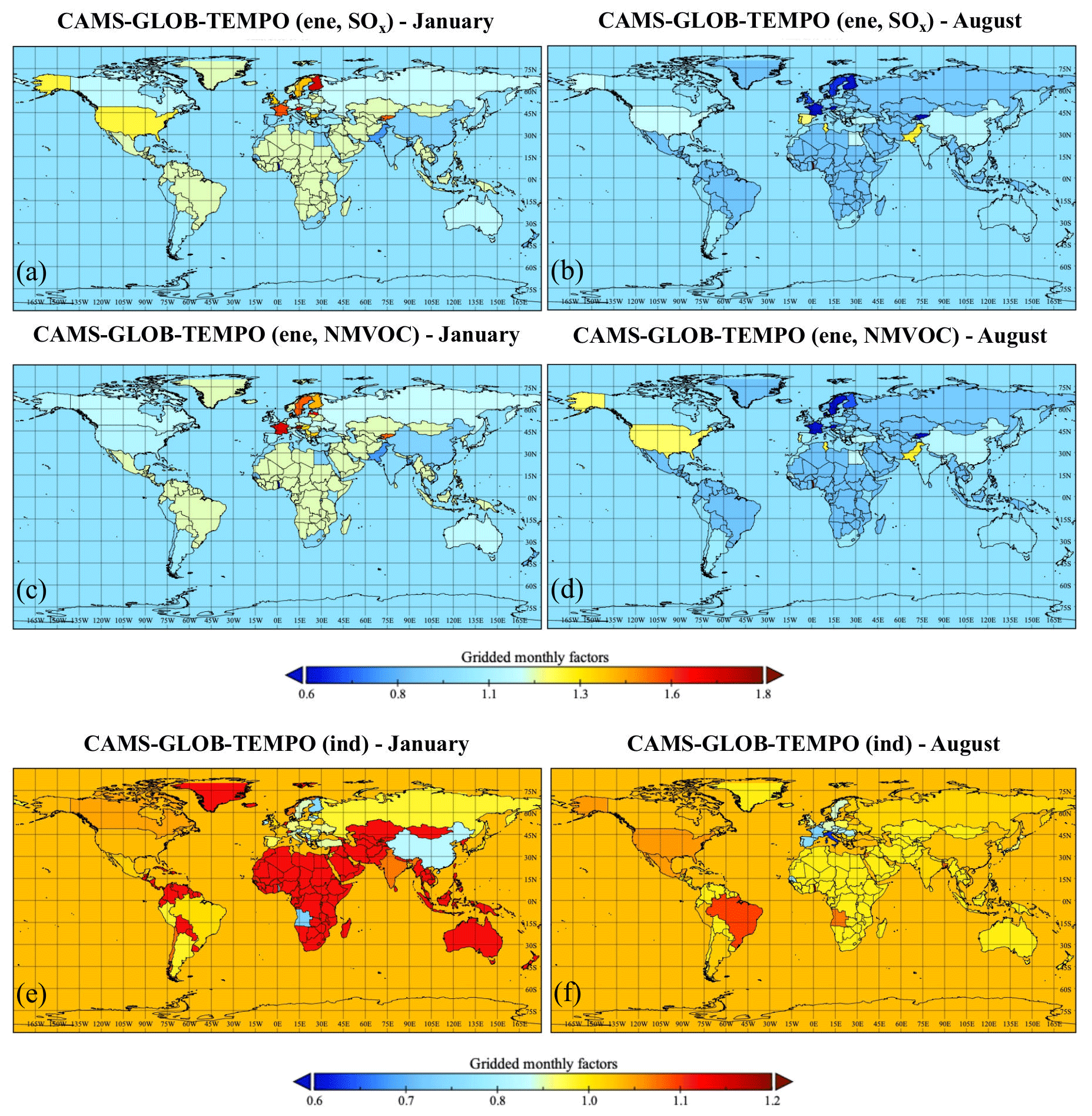
Figure 5CAMS-GLOB-TEMPO (0.1 × 0.1∘) monthly scale factor maps for SOx (a, b) and NMVOC (c, d) energy industry (ene) emissions and for manufacturing industry (ind) emissions (e, f) for the months of January and August. Administrative boundaries are derived from the Micro World Data Bank (MWDB2, 2011).
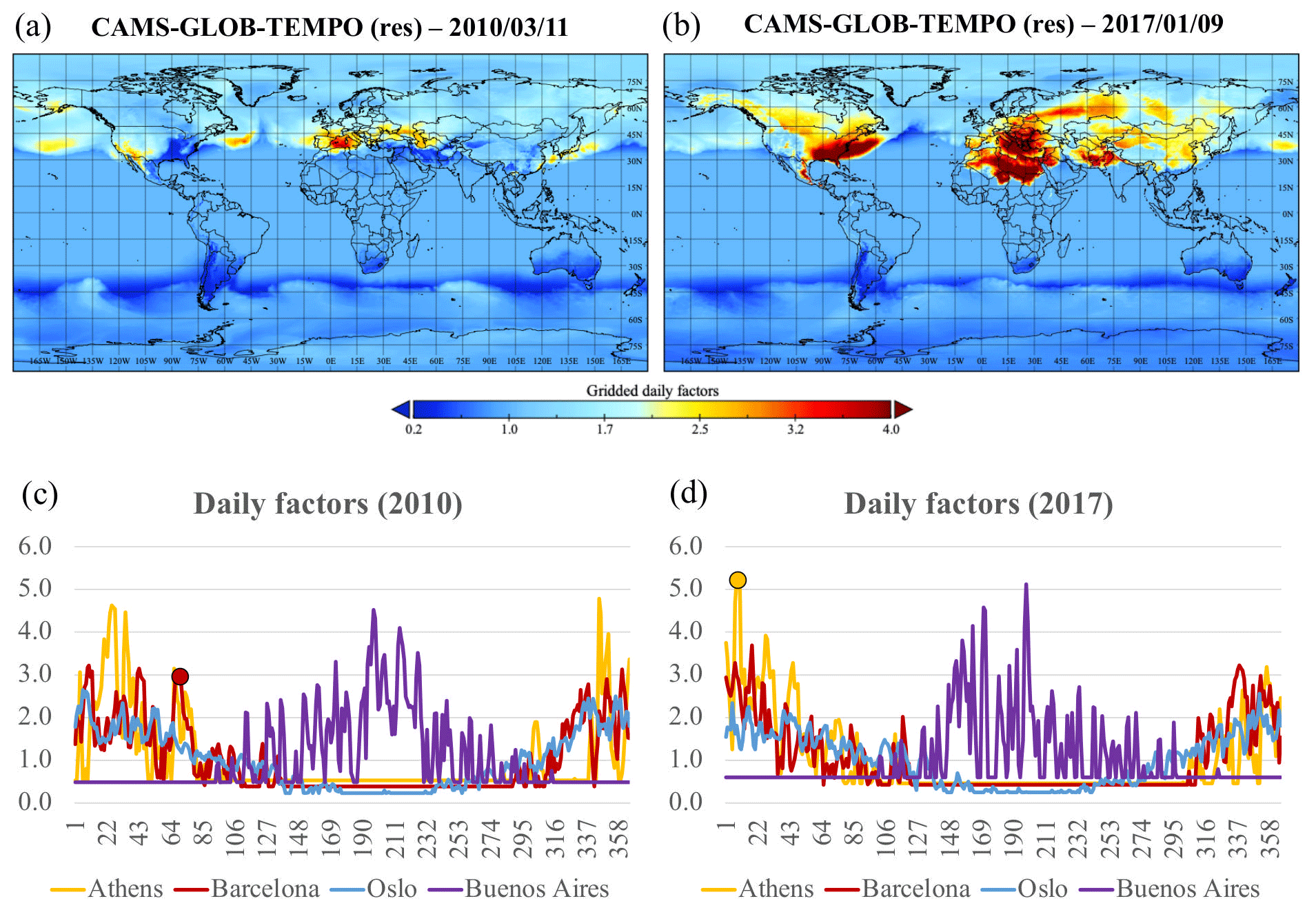
Figure 6CAMS-GLOB-TEMPO (0.1 × 0.1∘) daily-scale factor maps for residential and commercial (res) emissions for 11 March 2010 (a) and 9 January 2017 (b). Daily factors obtained over the cities of Athens, Barcelona, Buenos Aires and Oslo for 2010 (c) and 2017 (d). The red and yellow circles on the plots indicate the cold outbreaks experienced in Barcelona (11 March 2010) and Athens (9 January 2017), respectively. Administrative boundaries are derived from the Micro World Data Bank (MWDB2, 2011).
Figure 6 shows two examples of CAMS-GLOB-TEMPO gridded daily profiles for the residential and commercial sector along with the times series at four geographically or climatically different locations (i.e. Athens, Barcelona, Buenos Aires and Oslo) for the years 2010 and 2017. As expected, the largest factors occur in winter, and the lowest ones occur in summer at all four locations. According to the results, emissions in Athens, Barcelona or Buenos Aires can be 3 to 5 times higher during the cold periods (i.e. January in Barcelona and Athens and June in Argentina) than during warm periods (August in Barcelona and Athens and January in Argentina). In Oslo both the seasonal cycle and daily variability are less pronounced than in the other locations because the differences between daily and annual mean temperatures are generally lower. There is a large interannual variability in the four locations. In the winter of 2010, Barcelona experienced three cold outbreaks of similar intensity (in January, February and March), whereas in 2017 only one significant episode can be observed (mid-January). Similarly, in 2010 three major peaks are observed in Athens in mid-January, the beginning of February and mid-December, whereas in 2017 only one episode stands out above the rest. Results clearly highlight that extreme weather events can strongly affect the temporal profiles and thereby the resulting emissions.
Figure 7 shows examples of the 0.1 × 0.05∘ CAMS-REG-TEMPO gridded profiles constructed for the different road transport categories, including January and August (monthly) weights for gasoline CO exhaust emissions and both Friday and Sunday (weekly) and 09:00 and 20:00 (hourly weekday) weights for all traffic sources except NMVOC gasoline evaporation. The monthly gridded profiles clearly show the influence of outdoor temperature, with weight factors up to 2.5 times higher in January than in August in eastern Europe and Russia. The weekly profile maps clearly show the decrease in emissions from traffic during the weekend, especially in urban areas. The hourly profiles show the high levels of traffic activity during nighttime in some Mediterranean countries compared to central and northern European ones and also a clear distinction between urban and rural areas.
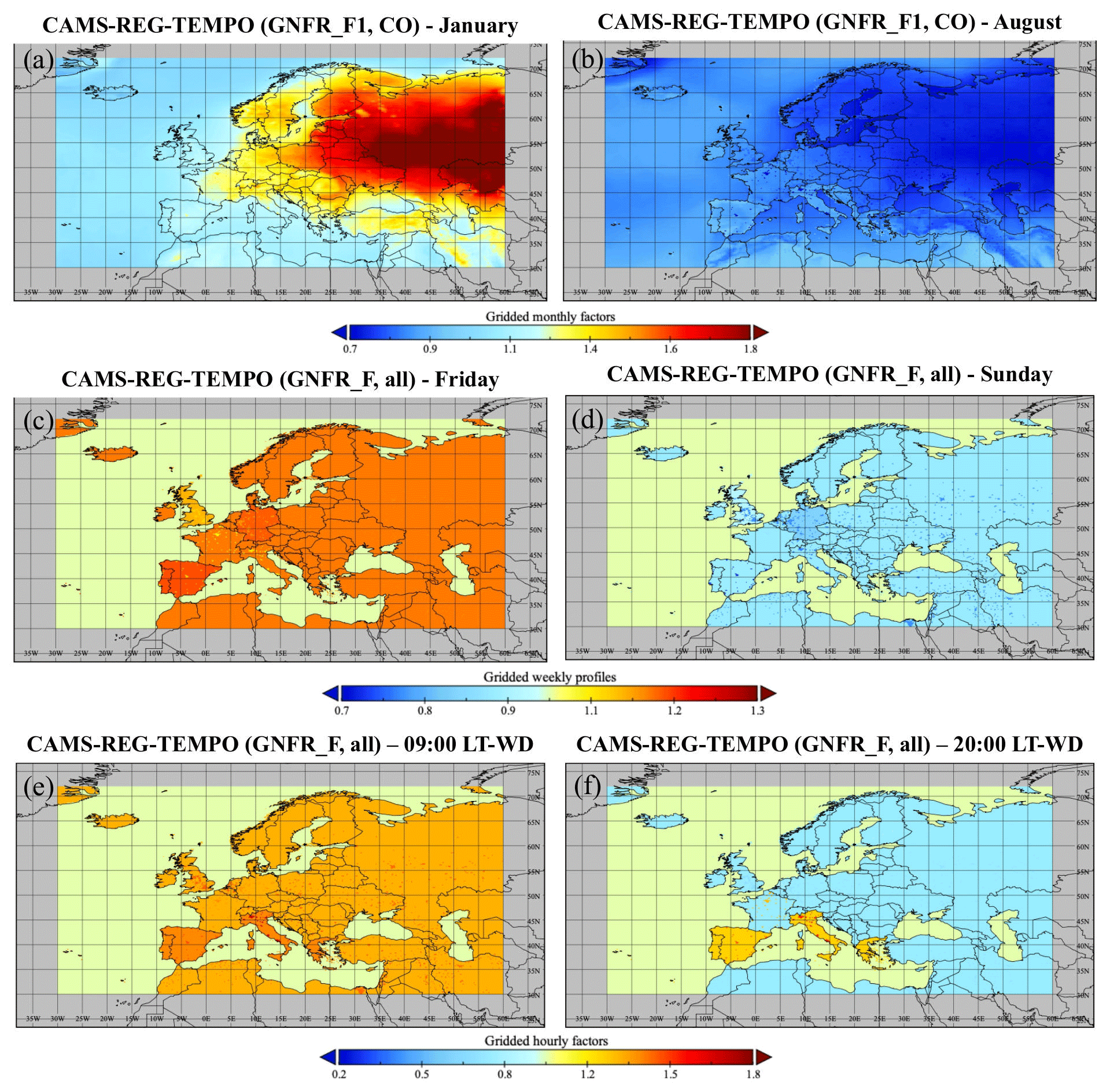
Figure 7CAMS-REG-TEMPO (0.1 × 0.05∘) monthly- (a, b), weekly- (c, d) and hourly-scale (e, f) factor maps. Monthly factors correspond to the meteorology-dependent profiles computed for CO exhaust gasoline emissions (GNFR_F1) for January and August (climatology of 2010–2017). Weekly factors are represented for Friday and Sunday. Hourly factors are represented for weekdays (WD) at 09:00 and 20:00 local time (LT). Administrative boundaries are derived from the Micro World Data Bank (MWDB2, 2011).

Figure 8CAMS-GLOB-TEMPO (0.1 × 0.1∘) monthly- (a, b) and daily-scale (c, d) factor maps for agriculture (agr) NH3 emissions and livestock (mma) NH3 and NOx emissions for April and November and 6 March and 16 July 2017, respectively. Daily factors for livestock emissions (mma) obtained over Spain and Argentina for 2010 and 2017 (e). Administrative boundaries are derived from the Micro World Data Bank (MWDB2, 2011).
Figure 8 shows examples of CAMS-GLOB-TEMPO profiles for the different agricultural emission sources, including April and November (monthly) weights for fertilizer NH3 emissions, daily (i.e. 6 March and 16 July 2017) weights for livestock NH3 and NOx emissions, and daily time series for livestock emissions over Spain and Argentina for 2010 and 2017. (Note the country daily times series are spatially aggregated, as the actual patterns are variable spatially.) Concerning the fertilizer monthly factors, it is observed that the spatial resolution is not homogeneous across the domain. This is due to the different spatial resolutions of the original datasets used to construct this gridded profile: the MASAGE_NH3 emission inventory is available at a resolution of 2×2.5∘, while the datasets used for China and the USA are reported at resolutions of 0.25×0.25∘ and 12 km × 12 km, respectively. Despite the coarse resolution, the profiles broadly capture the different seasonality in different parts of the world, with a peak of emissions occurring in April in Europe and in November in Latin America. For the livestock sector, the largest weight factors occur during the summer, and the lowest ones occur during the winter due to the temperature dependence. Nevertheless and in contrast to what is observed with the residential and commercial daily factors, the signal for livestock emissions is mostly seasonal, and the daily fluctuations are relatively small, which makes the interannual variability small.
3.1 Comparison to independent observational datasets
We compared the CAMS-TEMPO profiles to independent observational datasets. The comparison is mainly performed at the European level, as sufficient data could not be gathered to provide a robust comparison for other regions.
Figure 9 shows the CAMS-TEMPO monthly weight factors for SOx for the energy industry in Spain and manufacturing industry in Italy compared to two independent temporal profiles based on SOx measured emissions from all Spanish power plants (CIEMAT, Centro de Investigaciones Energéticas, Medioambientales y Tecnológicas, personal communication, 2018) and real-world measurements of industrial natural gas consumption provided by the European Network of Transmission System Operators for Gas (ENTSOG, 2020), respectively. Correlations between the two time series are high in both cases (i.e. r=0.84 and 0.61, respectively). In the case of the energy industry in Spain both profiles show minimum levels during spring and an increase during summer due to the intensive use of air-conditioning systems. In Italy, both manufacturing industry profiles present a strong decrease during August and December due to the summer and Christmas holidays.
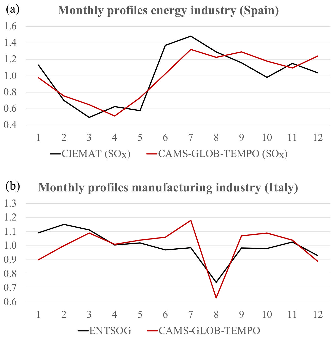
Figure 9(a) Comparison between monthly temporal factors for SOx energy industry emissions derived from power plant emission measurements (CIEMAT, personal communication, 2018) and reported by CAMS-GLOB-TEMPO for Spain. (b) Comparison between monthly temporal factors for manufacturing industry emissions derived from real-world measurements of industrial natural gas consumption (ENTSOG, 2020) and reported by CAMS-GLOB-TEMPO for Italy.
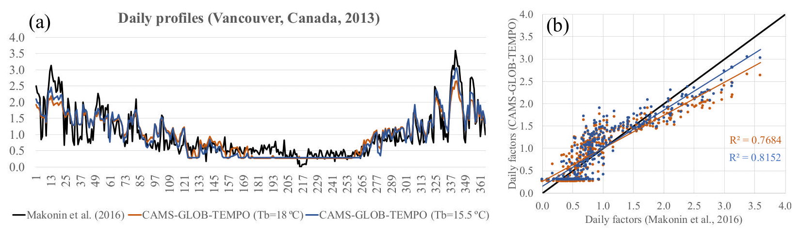
Figure 10(a) Comparison between daily temporal factors obtained in a location in Vancouver (Canada) for 2013 from real-world measurements of residential natural gas consumption (Makonin et al., 2016) and from the residential and commercial gridded temporal profiles reported by CAMS-GLOB-TEMPO. Two versions of the CAMS-GLOB-TEMPO temporal factors are shown as a function of the base temperature (Tb) assumed when applying the heating-degree-day approach (18 ∘C in orange and 15.5 ∘C in blue). (b) Scatterplot showing the trend lines and R2 values obtained from the comparison between measurement-based and CAMS-GLOB-TEMPO daily factors.
In Fig. 10 we compare our profiles for the residential sector with daily factors derived from minute-resolved measurements of natural gas from a residential house in Canada during 2013 (Makonin et al., 2016). We compared our daily factors estimated using the HDD approach for the grid cell closer to the house and considering two different values of Tb (18 and 15.5 ∘C). In both cases, CAMS-TEMPO reproduces the temporal variation of the locally measured profile. Both at the beginning and the end of the year, the measured and HDD-based profiles show similar maximum values, which correspond to the periods when outdoor temperature reached the minimum levels (not shown). The results also show that using Tb=15.5 ∘C we obtain a slightly higher correlation than when assuming Tb=18 ∘C (0.81 versus 0.76).
In Fig. 11 we compare the CAMS-REG-TEMPO road transport profiles to the temporal variation of air pollutant concentrations measured in Madrid, Milan, Barcelona and Berlin. CO and NO2 hourly concentrations were obtained from the European Environmental Agency (EEA) download service of validated and official air quality data (EEA, 2019). Four urban traffic stations highly influenced by road transport emissions were considered for the analysis: Escuelas Aguirre (Madrid); Milan Senato (Milan); Eixample (Barcelona); and Karl-Marx-Str. 76, Neukölln (Berlin).
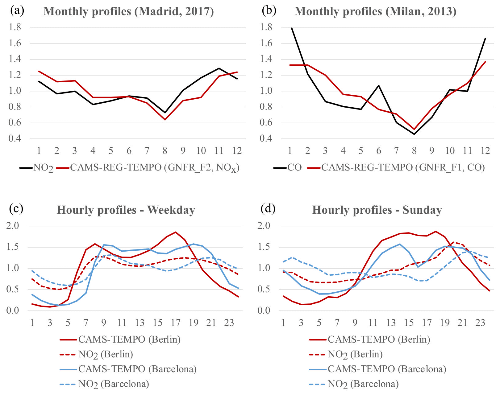
Figure 11Comparison between monthly variations of CAMS-REG-TEMPO profiles for NOx diesel exhaust emissions (GNFR_F2) and measured NO2 concentrations for the city of Madrid during 2017 (a). Comparison between monthly variations of the CAMS-REG-TEMPO profile for CO gasoline exhaust emissions (GNFR_F1) and measured CO concentrations for the city of Milan during 2013 (b). Hourly variation of CAMS-TEMPO GNFR_F profiles and NO2 concentrations during weekdays (c) and Sundays (d) for the cities of Barcelona and Berlin.
The monthly variability of CO and NO2 measured concentrations in Milan and Madrid were compared to the meteorology-dependent gridded monthly profiles created for CO GNFR_F1 (gasoline exhaust) and NOx GNFR_F2 (diesel exhaust) at these locations. Weight factors from the grid cells closest to each station were selected for the comparison. As shown in Fig. 11a and b, the traffic decrease occurring during summertime in Milan and Madrid is also reproduced in the CO and NO2 levels. At the same time, both the CAMS-REG-TEMPO profiles and the measurement-based profiles show a V shape, indicating higher emissions during winter due to the low temperatures. The correlation between the two times series is r=0.82 for Milan and r=0.74 for Madrid. We note that the seasonality of the CO and NO2 measurements may be also influenced by other factors, including meteorology and the influence of other emission sources such as residential combustion, and subsequently a perfect correlation between the two datasets cannot be expected.
Similarly, the hourly profiles proposed for urban locations in Spain and Germany during weekdays and Sundays were compared to the hourly variation of NO2 concentrations for Barcelona and Berlin (Fig. 11c and d). In all cases the hourly evolution of NO2 is mostly driven by variations accounted for in the CAMS-TEMPO profiles. For weekdays, the shift of the traffic morning and evening peaks observed between cities is also reproduced in NO2 concentrations. Traffic and NO2 levels in Berlin reach maximum levels between 07:00 and 08:00 LT, whereas in Barcelona the peak occurs between 08:00 and 09:00 LT. On the other hand, Sunday nighttime and morning NO2 concentrations (between 23:00 and 08:00 LT) are relative higher in Barcelona than in Berlin (in relative terms), which is related to the more intense traffic activity registered in the streets.
3.2 Comparison to other temporal profile datasets
We compared the CAMS-TEMPO profiles to the profiles reported by other existing datasets. The comparison is focussed on the profiles that are currently being used for air quality modelling purposes under the framework of CAMS, namely the global EDGARv4.3.2 (Janssens-Maenhout et al., 2019) monthly profiles (used in the CAMS global production) and the European EMEP (Simpson et al., 2012) and TNO (Denier van der Gon et al., 2011) profiles (used in CAMS regional production).
The comparison of monthly, weekly and hourly profiles for the energy industry sector in selected countries is shown in Fig. 12. It is worth noting that both TNO and EDGAR report the same profile for all countries. At the monthly level, significant differences are observed between CAMS-TEMPO and EDGAR in China and the USA. In both cases, the summer peak observed in CAMS-TEMPO (presumably due to the intensive use of air-conditioning systems) does not show up in the EDGAR profile. In the case of Romania, all profiles show important decreases but at different times of the year: April in CAMS-TEMPO (presumably due to the low use of heating and cooling devices), July in TNO and EDGAR, and September in EMEP. In the UK, the patterns between the different datasets are more similar, with all of them reproducing a V shape, except for the relatively flatter NMVOC emission profiles in CAMS-TEMPO. Concerning the weekly and hourly profiles, important discrepancies are observed between CAMS-TEMPO and the factors proposed by TNO and EMEP for certain countries. In the CAMS-TEMPO weekly profiles for Austria the intensity of the weekend decrease is relatively higher, while the hourly profiles for Spain are flatter than the ones reported by TNO and EMEP.
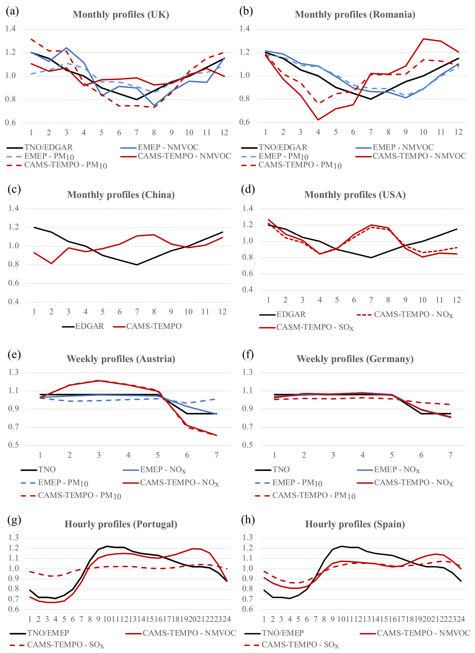
Figure 12Comparison of monthly (a, b), weekly (c, d) and hourly (e, f) profiles for energy industry emissions developed in the present work (CAMS-TEMPO) with profiles from EDGAR, EMEP and TNO for selected countries.
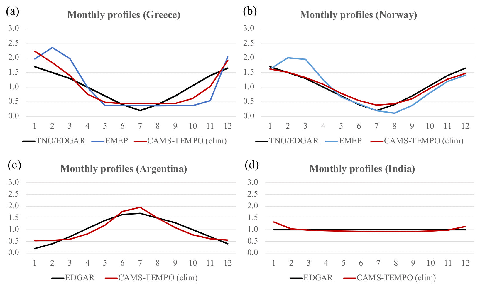
Figure 13Comparison of monthly profiles for residential and commercial combustion emissions developed in the present work (CAMS-TEMPO) with profiles from EDGAR, EMEP and TNO for selected countries. The CAMS-TEMPO profiles represent the climatological weight factors (clim) based on the average of each month over all the available years (2010–2017).
The comparison of monthly weight factors for the residential and combustion sector indicates generally low discrepancies between the different datasets (Fig. 13). The largest difference is observed in Greece, where both CAMS-TEMPO and EMEP allocate most of the emissions during wintertime, while TNO and EDGAR propose a smoother transition between this season of the year and spring and autumn. Both the EDGAR and CAMS-TEMPO datasets propose an almost flat profile for India, where residential fuel is mainly used for cooking activities, an activity that can be considered constant throughout the year. For the daily temporal disaggregation of emissions, TNO and EMEP propose a fixed weekly profile (not shown) which disregards the daily dynamics inferred by the heating-degree-day approach considered in CAMS-TEMPO (Fig. 6).
For road transport, the differences between CAMS-TEMPO and other datasets are quite significant. The monthly profiles reported by TNO, EMEP and EDGAR are almost flat, while the pollutant- and meteorology-dependent profiles developed in the present work suggest important decreases during summertime, especially for the case of CO (Fig. 14a). At the weekly level, the TNO profile is in line with most of the city-level constructed profiles, although in some cases differences in the intensity of the weekend decrease are observed (Fig. 4b). At the hourly level, the main discrepancies are observed when comparing TNO with the Saturday and NMVOC evaporative profiles of CAMS-TEMPO (Fig. 4d). It is worth noting that the hourly weekday profile constructed for Utrecht is almost perfectly correlated with TNO (R2=0.97). This is explained by the fact that the TNO profile was estimated using Dutch traffic data.

Figure 14Comparison of monthly profiles for road transport emissions developed in the present work (CAMS-TEMPO) with profiles from EDGAR, EMEP and TNO for selected countries and categories: CO gasoline exhaust (GNFR_F1, a), NOx diesel exhaust (GNFR_F2, b) and NMVOC non-exhaust (GNFR_F4, c).

Figure 15Comparison of monthly profiles for agricultural emissions developed in the present work (CAMS-TEMPO) with profiles from EDGAR, EMEP and TNO for selected countries and categories: NH3 livestock emissions in Europe (a) and China and India (b), NH3 other agricultural emissions in Europe (c) and China and India (d), and PM10 other agricultural emissions in Europe (e).
Figure 15 shows a comparison of the monthly profiles for the agricultural sector. All the datasets selected for comparison, except for TNO, propose a unique profile for all the different agricultural activities (i.e. livestock, use of fertilizers and agricultural-waste burning), which is equally applied to all emissions. The CAMS-TEMPO profiles constructed for NH3 fertilizer emissions show how the peak significantly varies among countries (i.e. May in China, June in India and April in Spain). In the case of India and China, these peaks are consistent with the NH3 satellite-derived seasonality shown by Warner et al. (2017). It is also worth noting the triple peak in Poland, which is related to the application timings of fertilizers (spring) and manure (summer and autumn) on crops (Werner et al., 2017). In contrast, the profiles reported by TNO and EMEP show a unique peak in April in all countries. In the case of NH3 from livestock, the profiles show a weaker seasonality, but relevant discrepancies in the intensities and occurrences of the emission peaks are also observed (i.e. EDGAR for India and EMEP for Spain). In the case of PM10 emissions related to agricultural-waste burning activities, the results suggest a good agreement between EMEP and CAMS-TEMPO, with most emissions occurring during autumn, after the harvesting period. On the other hand, the profile proposed by TNO presents a double peak, with a first one occurring during spring (March and April) and a second one during summer (August).
Gridded maps with all the temporal factors (monthly, weekly, daily and hourly) per sector and year are available as NetCDF (Network Common Data Format) files for the global domain at a resolution of 0.1 × 0.1∘ (CAMS-GLOB-TEMPOv2.1, https://doi.org/10.24380/ks45-9147, Guevara et al., 2020a), and the European regional domain (30∘ W–60∘ E and 30–72∘ N) at a resolution of 0.1 × 0.05∘ (CAMS-REG-TEMPOv2.1, https://doi.org/10.24380/1cx4-zy68, Guevara et al., 2020b) and can be accessed through the Emissions of atmospheric Compounds and Compilation of Ancillary Data (ECCAD) system with a login account (https://eccad.aeris-data.fr/, last access: February 2021). For review purposes, ECCAD has set up an anonymous repository where subsets of the CAMS-GLOB-TEMPOv2.1 and CAMS-REG-TEMPOv2.1 data can be accessed directly (https://www7.obs-mip.fr/eccad/essd-surf-emis-cams-tempo/, last access: February 2021). In addition, constructed fixed temporal profiles are available per sector and substance in Appendix A of this work.
This paper presents the CAMS-TEMPO dataset, a collection of monthly, weekly, daily and hourly emission temporal profiles for the priority air pollutants (NOx, SOx, NMVOC, NH3, CO, PM10 and PM2.5) and the greenhouse gases (CO2 and CH4) and each of the following anthropogenic source categories: energy industry, residential combustion, manufacturing industry, road transport (exhaust and non-exhaust processes), aviation (LTO cycles) and agriculture (i.e. use of fertilizers, livestock and agricultural-waste burning). Depending on the pollutant source and temporal resolution, the resulting profiles are reported as spatially invariant (i.e. a unique set of temporal weights for all the domain) or gridded values (i.e. temporal weights vary per grid cell). Multiple sources of information – including energy statistics and measured activity data, among others – and meteorology-dependent parametrizations have been collected and adapted to construct the profiles.
The CAMS-TEMPO profiles were designed to be combined with the global and regional anthropogenic emission inventories developed under the framework of Copernicus (CAMS-GLOB-ANT and CAMS-REG_AP/GHG, respectively) and to break down the original aggregated annual emissions to finer temporal resolutions (up to hourly). In order to ensure this combination, the developed temporal weight factors were constructed at a global 0.1 × 0.1∘ and regional 0.1 × 0.05∘ resolution following the domain descriptions and emission sector classification system defined in the each of the inventories.
There are several features that makes the CAMS-TEMPO profiles a major step when compared to the datasets currently being used for air quality modelling under the framework of CAMS:
-
Pollutant dependency. For some sectors, profiles were computed for all species independently in order to account for the variability of the activity patterns and the specific processes that drive their release to the atmosphere. As an example, a distinction was made between the temporal distribution of traffic emissions from non-exhaust PM mainly driven by traffic activity and non-exhaust NMVOC evaporation mainly driven by outdoor temperature.
-
Spatial variability. For nearly all sectors, the temporal profiles are made country- or even country- and region-specific in order to take into account the effects of e.g. different sociodemographic patterns and climatological conditions. For instance, differences between urban and rural traffic activity patterns are considered in the profiles constructed for road transport emissions.
-
Meteorological influence. For the residential and commercial combustion, road transport, and agriculture sector, the profiles were constructed using meteorology-dependent parametrizations (e.g. heating degree day and temperature effect on exhaust traffic emissions) that account for the emissions variability driven by temperature or wind speed. The resulting profiles are year-dependent and cover a time span that goes from 2010 to 2017.
Several CAMS-TEMPO profiles are analysed in this paper to illustrate their main characteristics and potential. Moreover, an intercomparison exercise of independent observational datasets (e.g. real-world measurements of natural gas consumption, emissions and pollutant concentrations) and other existing sets of temporal profiles was also performed. The comparison between CAMS-TEMPO temporal weight factors and the measurement-based profiles showed in general a high degree of correlation. Despite the scarcity of independent measurements, our comparison suggests a high level of representativeness of the developed profiles. On the other hand, the comparison to other sets of temporal profiles showed important discrepancies, especially for the traffic and agricultural sectors. This comparison highlights some shortcomings of the global and regional profiles currently used in the framework of CAMS, namely the omission of meteorological influences and the neglection of the temporal variation of emissions across sectors, species, and/or countries or regions.
It is important to highlight that the continuous growth of the open-data movement has been a key element for the successful development of the CAMS-TEMPO data. Services such as the European Open Data Portal (https://data.europa.eu/euodp/en/data, last access: February 2021) – and similar initiatives at the city level – or the ENTSO-E Transparency Platform (ENTSO-E, 2018) are delivering very valuable data for the development of emission-related databases.
5.1 Limitations of the dataset
The CAMS-TEMPO dataset provides an updated global and regional (European) picture of the temporal characterization of emissions by aggregated sectors. Despite all the efforts, there are, however, some limitations associated with the current version of the dataset that potential users of the CAMS-TEMPO should take into account.
First, the specificity of the computed profiles depends upon the degree of sectoral disaggregation used to report the original CAMS inventories. For instance, monthly profiles per industrial divisions could not be considered, since all manufacturing emissions are reported under a unique sector in both CAMS-GLOB-ANT and CAMS-REG_AP/GHG. Similarly, fuel-weighted profiles that are spatially aggregated to the national level were considered to be in the energy industry sector, as original emissions are not split by fuel type. On the other hand, the split by fuel type of traffic emissions in the CAMS-REG_AP/GHG inventory allowed for considering meteorological influences associated with e.g. CO gasoline and NOx diesel emissions, but specific traffic activity dynamics associated with light-duty and heavy-duty vehicles could not be accounted for.
A second limitation is related to the assumptions made when applying the heating-degree-day approach for the residential and commercial combustion sector. The computation of daily temporal factors was done considering a threshold temperature and a fraction of non-space-heating activities homogenous for all the world (15.5 ∘C and 0.2, respectively). Several studies have highlighted that these two values can vary across regions due to changes in local climate, building characteristics and sociodemographic aspects. For instance, Grythe et al. (2019) concluded that a lower threshold temperature value (i.e. 10 ∘C) may be more representative for Scandinavian countries, whereas Daioglou et al. (2012) indicated that in rural areas of developing regions (e.g. India, China and Brazil) the share of biomass used for cooking purposes can be larger than 80 %. Region-dependent HDD parameters should be considered in order to overcome this limitation.
Another important shortcoming of the current CAMS-TEMPO dataset is related to the scarcity of available information in developing regions (i.e. Africa, South America and Asia) to construct detailed profiles for the energy industry, manufacturing industry and road transport sectors. In the current version of the CAMS-TEMPO dataset, a simple gap-filling method has been implemented, which consists of mainly using the TNO European-based profiles when no national or local datasets are available. The rationale behind this choice is that the TNO profiles have been largely used and tested over the last decade in multiple international modelling exercises such as the Air Quality Model Evaluation International Initiative (AQMEII; Pouliot et al., 2015). However, TNO profiles are mostly based on western European data, and therefore the degree of representativeness for other world regions is a source of uncertainty. To address this constraint, the current gap-filling procedure will be reviewed in the future by constructing world region profiles for countries with geographical, climatological and/or behavioural similarities, following the approach presented by Crippa et al. (2020).
5.2 Future perspective
The CAMS-TEMPO dataset represents an effort to improve the temporal characterization of emission data to be used for atmospheric chemistry modelling. Future work will include the evaluation of these temporal profiles when used for modelling activities. Through close cooperation with air quality modellers, we expect to obtain feedback on the dataset as well as suggestions for future improvements. Besides that, a number of future updates have also been identified during the present work, including the following:
-
the extension of the year-dependent temporal profiles to be in line with the current time span considered in the CAMS-GLOB-ANT (2000–2018) and CAMS-REG_AP/GHG (2000–2017) inventories;
-
the development of new temporal profiles for certain sectors and pollutants that have not currently been considered, including CH4 emissions from agriculture (rice fields) and waste management (landfills); and
-
the refinement of the heating-degree-day approach considering region-dependent threshold temperature values.
Besides the identified updates, the investigation of monthly and seasonal changes of emissions using satellite data will also be explored in future work. Global and high-resolution observations of the atmospheric composition provided by missions such as the Copernicus Sentinel-5 Precursor (S5P) can be of great value to improve the description of the spatiotemporal distribution of emissions (Lorente et al., 2019). Finally, understanding and quantifying the impact of the COVID-19 lockdowns upon the temporal distribution of emissions will also be an important topic to be studied.
The CAMS-TEMPO profiles are distributed free of charge through the Emissions of atmospheric Compounds and Compilation of Ancillary Data (ECCAD) system (https://eccad.aeris-data.fr/, last access: February 2021).
Table A1Fixed monthly temporal profiles per domain, sector and pollutant. The definition of the sectors can be found in Tables 2 and 3.
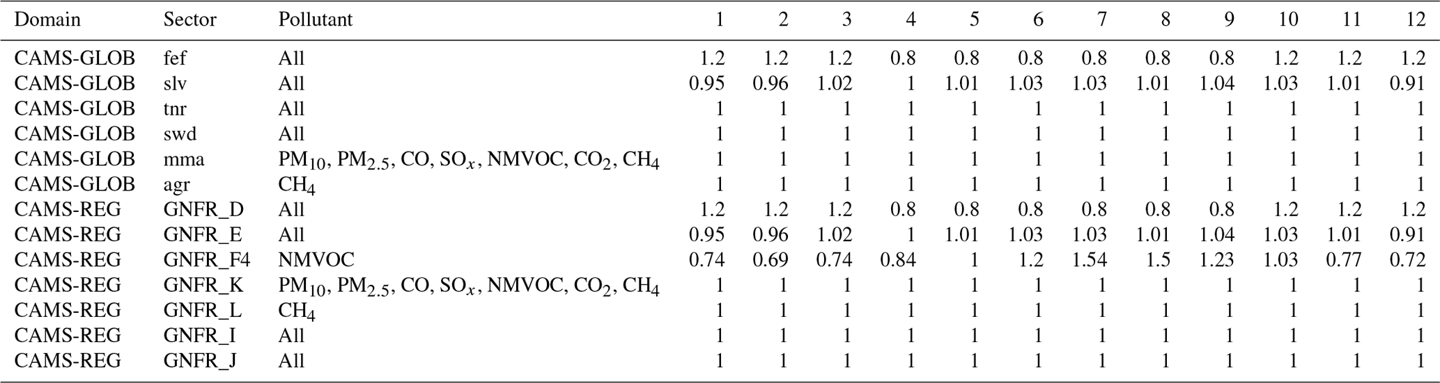
Table A2Fixed weekly temporal profiles per domain, sector and pollutant. The definition of the sectors can be found in Tables 2 and 3.
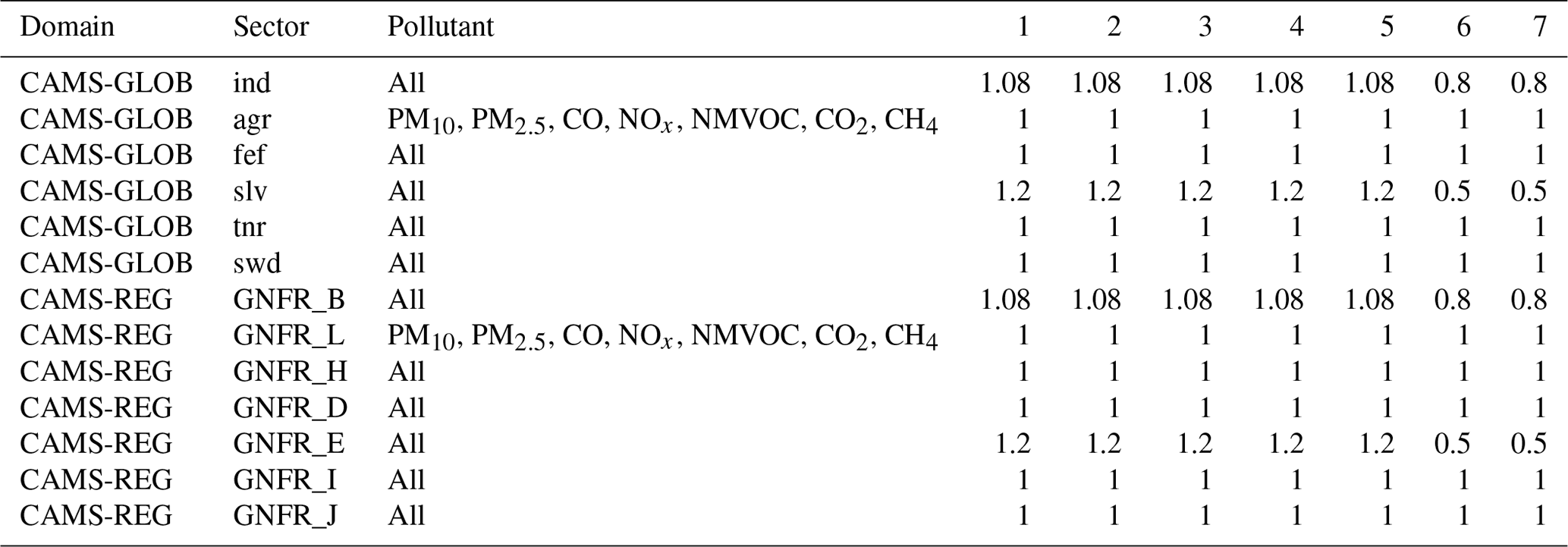
Table A3Fixed hourly temporal profiles per domain, sector and pollutant (part 1: 00:00–01:00 to 11:00–12:00). The definition of the sectors can be found in Tables 2 and 3.
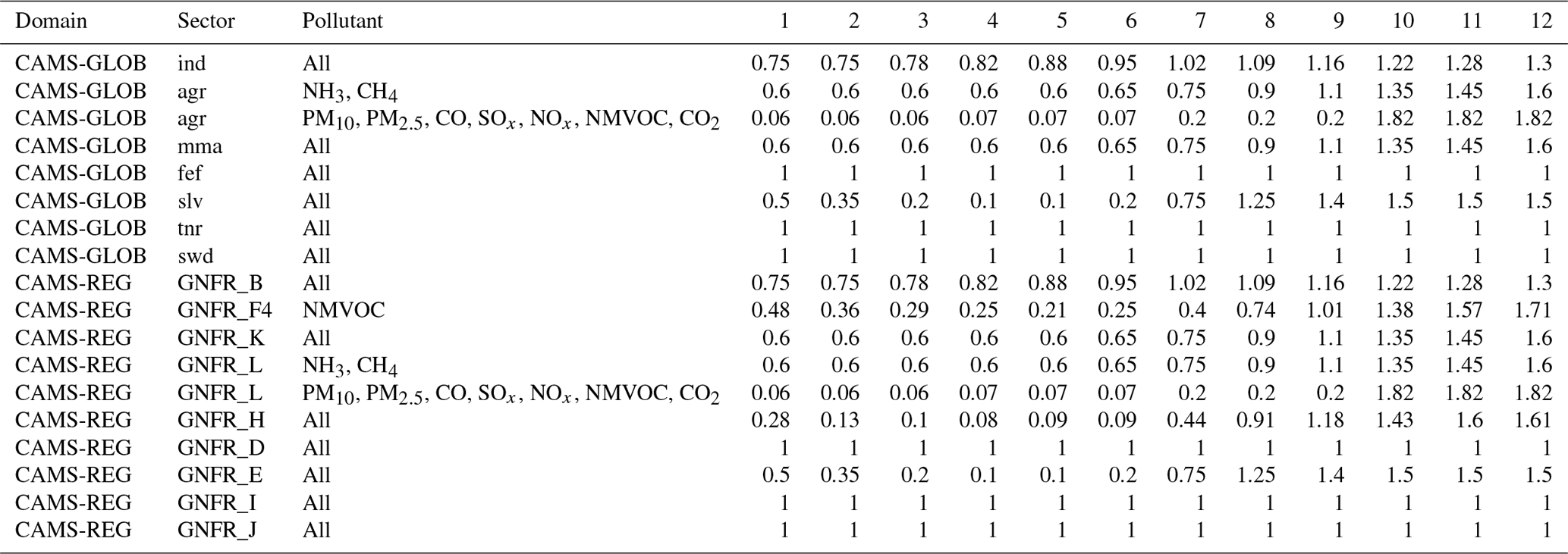
Table A4Fixed hourly temporal profiles per domain, sector and pollutant (part 2: 12:00–13:00 to 23:00–00:00). The definition of the sectors can be found in Tables 2 and 3.

The supplement related to this article is available online at: https://doi.org/10.5194/essd-13-367-2021-supplement.
MG conceived and coordinated the development of the CAMS-TEMPO profiles. CT helped construct the CAMS-TEMPO data files. NE and CG provided feedback on the construction of the global profiles and their combination with the CAMS-GLOB-ANT inventory. HDvdG and JK provided feedback on the construction of the European regional profiles and their combination with the CAMS-REG_AP/GHG inventory. SD processed and prepared the CAMS-TEMPO data files to make them available through the ECCAD system. OJ and CPGP helped conceive the CAMS-TEMPO dataset and supervised the work. MG prepared the paper with contributions from all co-authors.
The authors declare that they have no conflict of interest.
This article is part of the special issue “Surface emissions for atmospheric chemistry and air quality modelling”. It is not associated with a conference.
The present work was funded through the CAMS_81 (CAMS global and regional emissions) contract, coordinated by the Centre National de la Recherche Scientifique (CNRS, Claire Granier). The Copernicus Atmosphere Monitoring Service (CAMS, https://atmosphere.copernicus.eu/) is operated by the European Centre for Medium-Range Weather Forecasts on behalf of the European Commission as part of the Copernicus Programme. The study has also received support from the Ministerio de Ciencia, Innovación y Universidades (MICINN) as part of the BROWNING project (grant no. RTI2018-099894-B-I00) and NUTRIENT project (grant no. CGL2017-88911-R) and from the Agencia Estatal de Investigación (AEI) as part of the VITALISE project (grant no. PID2019-108086RA-I00 / AEI / 10.13039/501100011033). Carlos Pérez García-Pando acknowledges the European Research Council (grant no. 773051, FRAGMENT), the long-term support from the AXA Research Fund, and the support received through the Ramón y Cajal programme (grant no. RYC-2015-18690) of the MICINN. The authors acknowledge PRACE and RES for awarding access to MareNostrum at Barcelona Supercomputing Center. The authors are thankful to the Spanish Research Centre for Energy, Environment and Technology (CIEMAT) for sharing the databases of power plant emissions.
This research has been supported by the Copernicus Atmosphere Monitoring Service (CAMS), which is implemented by the European Centre for Medium-Range Weather Forecasts (ECMWF) on behalf of the European Commission (grant no. CAMS_81); the Ministerio de Ciencia, Innovación y Universidades (grant nos. RTI2018-099894-BI00, CGL2017-88911-R and RYC-2015- 18690); the Agencia Estatal de la Investigación (grant no. PID2019-108086-RA-I00 / AEI / 10.13039/501100011033); the AXA Research Fund; and the European Research Council (grant no. 773051, FRAGMENT).
This paper was edited by Mauricio Osses and reviewed by three anonymous referees.
AB: Barcelona City Council, Mobility data 2015, available at: https://www.barcelona.cat/mobilitat/sites/default/files/DB_2015.pdf (last access: January 2019), 2017.
Adolph, D.: Berechnung zeitlich hoch aufgelöster Emissionen der öffentlichen Strom- und Fernwärmeversorgung in Europa, Universität Gesamthochschule Essen, 1997.
Asman, W. A. H.: Ammonia Emission in Europe: Updated Emission and Emission Variations, Rep. 228471008, Natl. Inst. for Public Health and Environ. Prot., Bilthoven, The Netherlands, 1992.
Athanasopoulou, E., Speyer, O., Brunner, D., Vogel, H., Vogel, B., Mihalopoulos, N., and Gerasopoulos, E.: Changes in domestic heating fuel use in Greece: effects on atmospheric chemistry and radiation, Atmos. Chem. Phys., 17, 10597–10618, https://doi.org/10.5194/acp-17-10597-2017, 2017.
Backes, A., Aulinger, A., Bieser, J., Matthias, V., and Quante, M.: Ammonia emissions in Europe, part I: Development of a dynamical ammonia emission inventory, Atmos. Environ., 131, 55–66, https://doi.org/10.1016/j.atmosenv.2016.01.041, 2016.
BASt: Federal Highway Research Institute, Automatic counting stations on highways and federal highways, available at: https://www.bast.de/BASt_2017/DE/Verkehrstechnik/Fachthemen/v2-verkehrszaehlung/zaehl_node.html, last access: April 2018 (in German).
Bieser, J., Aulinger, A., Matthias, V., Quante, M., and Builtjes, P.: SMOKE for Europe – adaptation, modification and evaluation of a comprehensive emission model for Europe, Geosci. Model Dev., 4, 47–68, https://doi.org/10.5194/gmd-4-47-2011, 2011.
Board: Board of Governors of the Federal Reserve System, Industrial Production: Manufacturing (SIC) [IPMANSICS], retrieved from FRED, Federal Reserve Bank of St. Louis, available at: https://fred.stlouisfed.org/series/IPMANSICS, last access: October 2020.
Bonjour, S., Adair-Rohani, H., Wolf, J., Bruce, N. G., Mehta, S., Pruss-Ustun, A., Lahiff, M., Rehfuess, E. A., Mishra, V., and Smith, K. R.: Solid fuel use for household cooking: country and regional estimates for, Environ. Health Persp., 121, 784–790, https://doi.org/10.1289/ehp.1205987, 2013.
Borge, R., Lumbreras, J., and Rodríguez, E.: Development of a high-resolution emission inventory for Spain using the SMOKE modelling system: A case study for the years 2000 and 2010, Environ. Model. Softw., 23, 1026–1044, https://doi.org/10.1016/j.envsoft.2007.11.002, 2008.
Cai, H. and Xie, S.: Traffic-related air pollution modeling during the 2008 Beijing olympic games: the effects of an odd-even day traffic restriction scheme, Sci. Total. Environ., 409, 1935–1948, https://doi.org/10.1016/j.scitotenv.2011.01.025, 2011.
Carter, E., Archer-Nicholls, S., Ni, K., Lai, A. M., Niu, H., Secrest, M. H., Sauer, S. M., Schauer, J.J., Ezzati, M., Wiedinmyer, C., Yang, X., and Baumgartner, J.: Seasonal and Diurnal Air Pollution from Residential Cooking and Space Heating in the Eastern Tibetan Plateau, Environ. Sci. Technol., 50, 8353–8361, https://doi.org/10.1021/acs.est.6b00082, 2016.
Copernicus Climate Change Service (C3S): ERA5: Fifth generation of ECMWF atmospheric reanalyses of the global climate, Copernicus Climate Change Service Climate Data Store (CDS), available at: https://cds.climate.copernicus.eu/cdsapp#!/home, (last access: July 2019) 2017.
Copenhagen data: Copenhagen city open data portal, Permanent Traffic Counting, available at: https://portal.opendata.dk/dataset/faste-trafiktaellinger, last access: February 2018 (in Danish).
Crippa, M., Guizzardi, D., Muntean, M., Schaaf, E., Dentener, F., van Aardenne, J. A., Monni, S., Doering, U., Olivier, J. G. J., Pagliari, V., and Janssens-Maenhout, G.: Gridded emissions of air pollutants for the period 1970–2012 within EDGAR v4.3.2, Earth Syst. Sci. Data, 10, 1987–2013, https://doi.org/10.5194/essd-10-1987-2018, 2018.
Crippa, M., Solazzo, E., Huang, G., Guizzardi, D., Koffi, E., Muntean, M., Schieberle, C., Friedrich, R., and Janssens-Maenhout, G.: High resolution temporal profiles in the Emissions Database for Global Atmospheric Research, Sci. Data, 7, 121, https://doi.org/10.1038/s41597-020-0462-2, 2020.
Daioglou, V., Van Ruijven, B. V., and Van Vuuren, D. P.: Model projection for household energy use in developing countries, Energy, 37, 6011–6615, https://doi.org/10.1016/j.energy.2011.10.044, 2012.
Denier van der Gon, H. A. C., Hendriks, C., Kuenen, J., Segers, A., and Visschedijk, A. J. H.: Description of current temporal emission patterns and sensitivity of predicted AQ for temporal emission patterns, EU FP7 MACC deliverable report D_D-EMIS_1.3, available at: https://atmosphere.copernicus.eu/sites/default/files/2019-07/MACC_TNO_del_1_3_v2.pdf (last access: February 2021), 2011.
Ebel, A., Friedrich, R., and Rodhe, H.: GENEMIS: Assessment, Improvement, and Temporal and Spatial Disaggregation of European Emission Data, in Tropospheric Modelling and Emission Estimation: Chemical Transport and Emission Modelling on Regional, Global and Urban Scales, edited by: Ebel, A., Friedrich, R., and Rodhe, H., Springer Berlin Heidelberg, Berlin, Heidelberg, 181–214, https://doi.org/10.1007/978-3-662-03470-5_6, 1997.
EEA: Download service of air quality data, available at: http://discomap.eea.europa.eu/map/fme/AirQualityExport.htm (last access: January 2019), 2019.
EMEP/EEA: Air pollutant emission inventory guidebook 2016, Technical guidance to prepare national emission inventories, EEA Report No 21/2016, available at: https://www.eea.europa.eu/publications/emep-eea-guidebook-2016 (last access: July 2019), 2016.
EMEP/CEIP: Present state of emission data, available at: https://www.ceip.at/webdab-emission-database/reported-emissiondata (last access: February 2021), 2019.
Eurostat: Energy consumption in households, available at: https://ec.europa.eu/eurostat/statistics-explained/index.php/Energy_consumption_in_households, last access: May 2018.
Eurostat: Airport traffic data by reporting airport and airlines, available at: https://ec.europa.eu/eurostat/web/products-datasets/-/avia_tf_apal (last access: February 2021), 2019.
Elguindi, N., Darras, S., Granier, C., and Guevara, M: The CAMS global anthropogenic emissions (CAMS-GLOB-ANT), Copernicus Atmospheric Monitoring Service, ECCAD, https://doi.org/10.24380/fw9g-2t24, 2020a.
Elguindi, N., Granier, C., Stavrakou, T.,Darras, S., Bauwens, M., Cao, H., Chen, C., Denier van der Gon, H. A. C., Dubovik, O., Fu, T. M., Henze, D. K., Jiang, Z., Keita, S., Kuenen, J. J. P., Kurokawa, J., Liousse, C., Miyazaki, K., Muller, J.-F., Qu, Z., Solmon, F., and Zheng, B.: Intercomparison of magnitudes and trends in anthropogenic surface emissions from bottom-up inventories, top-down estimates, and emission scenarios, Earths Future, 8, e2020EF001520, https://doi.org/10.1029/2020EF001520, 2020b.
ENTSO-E: Transparency Platform, available at: https://transparency.entsoe.eu/, last access: May 2018.
ENTSOG: Transparency platform, available at: https://transparency.entsog.eu/#/map, last access: March 2020.
Fameli, K. M. and Assimakopoulos, V. D.: Development of a road transport emission inventory for Greece and the Greater Athens Area: effects of important parameters, Sci. Total Environ., 505, 770–786, https://doi.org/10.1016/j.scitotenv.2014.10.015, 2015.
Finstad, A., Flugsrud, K., Haakonsen, G., and Aasestad, K.: Wood consumption, fire habits and particulate matter, Results from Folke and housing census 2001, Living Conditions Survey 2002 and Survey of wood consumption and firing habits in Oslo 2002 Statistics Norway, Rapporter 2004/5, 2004 (in Norwegian).
Florczyk, A. J., Corbane, C., Ehrlich, D., Freire, S., Kemper, T., Maffenini, L., Melchiorri, M., Pesaresi, M., Politis, P., Schiavina, M., Sabo, F., and Zanchetta, L.: GHSL Data Package 2019, EUR 29788EN, Publications Office of the European Union, Luxembourg, https://doi.org/10.2760/062975, 2019.
Friedrich, R. and Reis, S.: Emissions of Air Pollutants – Measurements, Calculation, Uncertainties – Results from the EUROTRAC-2 Subproject GENEMIS, Springer Publishers, Berlin, Heidelberg, Germany, 2004.
GADM: Database of Global Administrative Areas, available at: http://www.gadm.org, last access: July 2020.
Galmarini, S., Koffi, B., Solazzo, E., Keating, T., Hogrefe, C., Schulz, M., Benedictow, A., Griesfeller, J. J., Janssens-Maenhout, G., Carmichael, G., Fu, J., and Dentener, F.: Technical note: Coordination and harmonization of the multi-scale, multi-model activities HTAP2, AQMEII3, and MICS-Asia3: simulations, emission inventories, boundary conditions, and model output formats, Atmos. Chem. Phys., 17, 1543–1555, https://doi.org/10.5194/acp-17-1543-2017, 2017.
GovUK: Road traffic statistics information, available at: https://www.gov.uk/government/collections/road-traffic-statistics, last access: March 2018.
Grange, S. K., Farren, N. J., Vaughan, A. R., Rose, R. A., and Carslaw, D. C.: Strong Temperature Dependence for LightDuty Diesel Vehicle NOx Emissions, Environ. Sci. Technol., 53, 6587–6596, https://doi.org/10.1021/acs.est.9b01024, 2019.
Granier, C., Bessagnet, B., Bond, T., D'Angiola, A., van der Gon, H. D., Frost, G. J., Heil, A., Kaiser, J. W., Kinne, S., Klimont, Z., Kloster, S., Lamarque, J. F., Liousse, C., Masui, T., Meleux, F., Mieville, A., Ohara, T., Raut, J. C., Riahi, K., Schultz, M.G., Smith, S. J., Thompson, A., van Aardenne, J., van der Werf, G. R., and van Vuuren, D. P.: Evolution of anthropogenic and biomass burning emissions of air pollutants at global and regional scales during the 1980–2010 period, Climatic Change, 109, 163–190, https://doi.org/10.1007/s10584-011-0154-1, 2011.
Granier, C., Darras, S., Denier van der Gon, H. A. C., Doubalova, J., Elguindi, N., Galle, B., Gauss, M., Guevara, M., Jalkanen, J.-P., Kuenen, J., Liousse, C., Quack, B., Simpson, D., and Sindelarova, K.: The Copernicus Atmosphere Monitoring Service global and regional emissions (April 2019 version), Copernicus Atmosphere Monitoring Service (CAMS) report, 2019, https://doi.org/10.24380/d0bn-kx16, 2019.
Gröndahl, T., Makkonen, J., Myllynen, M., Niemi, J., and Tuomi, S.: Use of fireplaces and discharges from small houses in the Helsinki metropolitan area, HSY publications, available at: https://www.tts.fi/files/874/meti737.pdf (last access:February 2021), 2010.
Grythe, H., Lopez-Aparicio, S., Vogt, M., Vo Thanh, D., Hak, C., Halse, A. K., Hamer, P., and Sousa Santos, G.: The MetVed model: development and evaluation of emissions from residential wood combustion at high spatio-temporal resolution in Norway, Atmos. Chem. Phys., 19, 10217–10237, https://doi.org/10.5194/acp-19-10217-2019, 2019.
Guevara, M., Tena, C., Porquet, M., Jorba, O., and Pérez García-Pando, C.: HERMESv3, a stand-alone multi-scale atmospheric emission modelling framework – Part 1: global and regional module, Geosci. Model Dev., 12, 1885–1907, https://doi.org/10.5194/gmd-12-1885-2019, 2019.
Guevara, M., Jorba, O., Tena, C., Denier van der Gon, H., Kuenen, J., Elguindi, N., Darras, S., Granier, C., and Pérez García-Pando, C.: Copernicus Atmosphere Monitoring Service TEMPOral profiles for the Global domain version 2.1 (CAMS-GLOB-TEMPOv2.1), Copernicus Atmosphere Monitoring Service, ECCAD, https://doi.org/10.24380/ks45-9147, 2020a.
Guevara, M., Jorba, O., Tena, C., Denier van der Gon, H., Kuenen, J., Elguindi, N., Darras, S., Granier, C., and Pérez García-Pando, C.: Copernicus Atmosphere Monitoring Service TEMPOral profiles for the regional European domain version 2.1 (CAMS-REG-TEMPOv2.1), Copernicus Atmosphere Monitoring Service, ECCAD, https://doi.org/10.24380/1cx4-zy68, 2020b.
Guevara, M., Tena, C., Porquet, M., Jorba, O., and Pérez García-Pando, C.: HERMESv3, a stand-alone multi-scale atmospheric emission modelling framework – Part 2: The bottom–up module, Geosci. Model Dev., 13, 873–903, https://doi.org/10.5194/gmd-13-873-2020, 2020c.
Gurney, K. R., Patarasuk, R., Liang, J., Song, Y., O'Keeffe, D., Rao, P., Whetstone, J. R., Duren, R. M., Eldering, A., and Miller, C.: The Hestia fossil fuel CO2 emissions data product for the Los Angeles megacity (Hestia-LA), Earth Syst. Sci. Data, 11, 1309–1335, https://doi.org/10.5194/essd-11-1309-2019, 2019.
Gyldenkærne, S., Skjøth, C. A, Hertel, O., and Ellermann, T.: Adynamical ammonia emission parameterization for use in air pollution models, J. Geophys. Res., 110, D07108, https://doi.org/10.1029/2004JD005459, 2005.
Hirth, L., Mühlenpfordt, J., and Bulkeley, M.: The ENTSO-E Transparency Platform – A review of Europe's most ambitious electricity data platform, Appl. Energy, 225, 1054–1067, https://doi.org/10.1016/j.apenergy.2018.04.048, 2018.
Hoesly, R. M., Smith, S. J., Feng, L., Klimont, Z., Janssens-Maenhout, G., Pitkanen, T., Seibert, J. J., Vu, L., Andres, R. J., Bolt, R. M., Bond, T. C., Dawidowski, L., Kholod, N., Kurokawa, J.-I., Li, M., Liu, L., Lu, Z., Moura, M. C. P., O'Rourke, P. R., and Zhang, Q.: Historical (1750–2014) anthropogenic emissions of reactive gases and aerosols from the Community Emissions Data System (CEDS), Geosci. Model Dev., 11, 369–408, https://doi.org/10.5194/gmd-11-369-2018, 2018.
Huang, G., Brook, R., Crippa, M., Janssens-Maenhout, G., Schieberle, C., Dore, C., Guizzardi, D., Muntean, M., Schaaf, E., and Friedrich, R.: Speciation of anthropogenic emissions of non-methane volatile organic compounds: a global gridded data set for 1970–2012, Atmos. Chem. Phys., 17, 7683–7701, https://doi.org/10.5194/acp-17-7683-2017, 2017.
IEA: Electricity Statistics, available at: https://www.iea.org/reports/monthly-electricity-statistics, last access: February 2021.
INE: Spanish Statistical Office, Industrial production, available at: https://www.ine.es/en/prensa/ipi_prensa_en.htm, last access: May 2018.
IPCC: 2006 IPCC Guidelines for National Greenhouse Gas Inventories, Prepared by the National Greenhouse Gas Inventories Programme, edited by: Eggleston H. S., Buendia L., Miwa K., Ngara T., and Tanabe K., IGES, Japan, 2006.
ISTAT: Italian National Institute of Statistics, Industrial production, available at: https://www.istat.it/en/archive/industrial+production, last access: June 2018.
James, K. M., Blunden, J., Rumsey, I. C., and Aneja, V. P.: Characterizing ammonia emissions from a commercial mechanically ventilated swine finishing facility and an anaerobic waste lagoon in North Carolina, Atmos. Pollut. Res., 3, 279–288, https://doi.org/10.5094/APR.2012.031, 2012.
Janssens-Maenhout, G., Crippa, M., Guizzardi, D., Muntean, M., Schaaf, E., Dentener, F., Bergamaschi, P., Pagliari, V., Olivier, J. G. J., Peters, J. A. H. W., van Aardenne, J. A., Monni, S., Doering, U., Petrescu, A. M. R., Solazzo, E., and Oreggioni, G. D.: EDGAR v4.3.2 Global Atlas of the three major greenhouse gas emissions for the period 1970–2012, Earth Syst. Sci. Data, 11, 959–1002, https://doi.org/10.5194/essd-11-959-2019, 2019.
Johansson, L., Jalkanen, J.-P., and Kukkonen, J.: Global assessment of shipping emissions in 2015 on a high spatial and temporal resolution, Atmos. Environ., 167, 403–415, https://doi.org/10.1016/j.atmosenv.2017.08.042, 2017.
Keller, M., Hausberger, S., Matzer, C., Wuthrich, P., and Notter, B.: HBEFA version 3.3. Background documentation, available at: https://www.hbefa.net/e/documents/HBEFA33_Documentation_20170425.pdf (last access: February 2021), 2017.
Klimont, Z., Kupiainen, K., Heyes, C., Purohit, P., Cofala, J., Rafaj, P., Borken-Kleefeld, J., and Schöpp, W., 2017. Global anthropogenic emissions of particulate matter including black carbon, Atmos. Chem. Phys., 17, 8681-8723, https://doi.org/10.5194/acp-17-8681-2017.
Kuenen, J. J. P., Visschedijk, A. J. H., Jozwicka, M., and Denier van der Gon, H. A. C.: TNO-MACC_II emission inventory; a multi-year (2003–2009) consistent high-resolution European emission inventory for air quality modelling, Atmos. Chem. Phys., 14, 10963–10976, https://doi.org/10.5194/acp-14-10963-2014, 2014.
Kuenen, J. J. P., Dellaert, S. N. C., Visschedijk, A. J. H., and Denier van der Gon, H. A. C.: CAMS -REG-v4: a state-of-the-art high-resolution European emission inventory for air quality and greenhouse gas modelling, in preparation, 2021.
Li, M., Zhang, Q., Kurokawa, J.-I., Woo, J.-H., He, K., Lu, Z., Ohara, T., Song, Y., Streets, D. G., Carmichael, G. R., Cheng, Y., Hong, C., Huo, H., Jiang, X., Kang, S., Liu, F., Su, H., and Zheng, B.: MIX: a mosaic Asian anthropogenic emission inventory under the international collaboration framework of the MICS-Asia and HTAP, Atmos. Chem. Phys., 17, 935–963, https://doi.org/10.5194/acp-17-935-2017, 2017.
Lorente, A., Boersma, K., Eskes, H., Veefkind, J. P., Van Geffen, J. H. G. M., De Zeeuw, M., Denier van der Gon, H., Beirle, S., and Krol, M. C.: Quantification of nitrogen oxides emissions from build-up of pollution over Paris with TROPOMI, Sci. Rep.-UK, 9, 20033, https://doi.org/10.1038/s41598-019-56428-5, 2019.
Madrid data: Madrid city open data portal, Traffic, Historic traffic data since 2013, available at: https://datos.madrid.es/sites/v/index.jsp?vgnextoid=33cb30c367e78410VgnVCM1000000b205a0aRCRD&vgnextchannel=374512b9ace9f310VgnVCM100000171f5a0aRCRD, last access: April 2018 (in Spanish).
Makonin, S., Ellert, B., Bajic, I. V., and Popowich, F.: AMPds2-Almanac of Minutely Power dataset: Electricity, water, and natural gas consumption of a residential house in Canada from 2012 to 2014, Sci. Data, 3, 160037, https://doi.org/10.1038/sdata.2016.37, 2016.
Mareckova, K., Wankmueller, R., Moosmann, L., and Pinterits, M.: Inventory Review 2013: Review of Emission Data reported under the LRTAP Convention and NEC Directive, Stage 1 and 2 review, Status of Gridded Data and LPS Data, STATUS Report 1/2013, Umweltbundesamt GmbH, Vienna, Austria, 2013.
Mareckova, K., Pinterits, M., Ullrich, B., Wankmueller, R., and Mandl, N.: Inventory review 2017, Review of emission data reported under the LRTAP Convention and the NEC Directive Stage 1 and 2 review, Status of gridded and LPS data, Technical Report CEIP 2/2017, Umweltbundesamt GmbH, Vienna, Austria, 2017.
Markakis, K., Poupkou, A., Melas, D., Tzoumaka, P., and Petrakakis, M.: A computational approach based on GIS technology for the development of an anthropogenic emission inventory of gaseous pollutants in Greece, Water Air Soil Pollut., 207, 157–180, https://doi.org/10.1007/s11270-009-0126-5, 2010.
MBS: Monthly Bulletin of Statistics Online, available at: https://unstats.un.org/unsd/mbs/, last access: March 2018.
McDonald, B. C., McBride, Z. C., Martin, E. W., and Harley, R. A.: High resolution mapping of motor vehicle carbon dioxide emissions, J. Geophys. Res. Atmos., 119, 5283–5298, https://doi.org/10.1002/2013JD021219, 2014.
Melbourne data: Melbourne's Open Data Platform, Traffic Count Vehicle Classification 2014–2017, available at: https://data.melbourne.vic.gov.au/Transport-Movement/Traffic-Count-Vehicle-Classification-2014-2017/qksr-hqee, last access: January 2019.
Menut, L., Goussebaile, A., Bessagnet, B., Khvorostiyanov, D., and Ung, A.: Impact of realistic hourly emissions profiles on air pollutants concentrations modelled with CHIMERE, Atmos. Environ., 49, 233–244, https://doi.org/10.1016/j.atmosenv.2011.11.057, 2012.
Milano data: Milano city open data portal, Area C traffic reporting, available at: https://dati.comune.milano.it/, last access: February 2021.
Mu, M., Randerson, J. T., van der Werf, G. R., Giglio, L., Kasibhatla, P., Morton, D., Collatz, G. J., DeFries, R. S., Hyer, E. J., Prins, E. M., Griffith, D. W. T., Wunch, D., Toon, G. C., Sherlock, V., and Wennberg, P. O.: Daily and 3-hourly variability in global fire emissions and consequences for atmospheric model predictions of carbon monoxide, J. Geophys. Res.-Atmos., 116, D24303, https://doi.org/10.1029/2011JD016245, 2011.
Mues, A., Kuenen, J., Hendriks, C., Manders, A., Segers, A., Scholz, Y., Hueglin, C., Builtjes, P., and Schaap, M.: Sensitivity of air pollution simulations with LOTOS-EUROS to the temporal distribution of anthropogenic emissions, Atmos. Chem. Phys., 14, 939–955, https://doi.org/10.5194/acp-14-939-2014, 2014.
MWDB2: Micro World Data Bank 2, available at: http://microworld-db-2.sourceforge.net/, (last access: July 2020), 2011.
Nassar, R., Napier-Linton, L., Gurney, K. R., Andres, R. J., Oda, T., Vogel, F. R., and Deng, F.: Improving the temporal and spatial distribution of CO2 emissions from global fossil fuel emission data sets, J. Geophys. Res., 118, 917–933, https://doi.org/10.1029/2012jd018196, 2013.
New York City data: New York city open data portal, Traffic Volume Counts (2014–2018), available at: https://data.cityofnewyork.us/Transportation/Traffic-Volume-Counts-2014-2018-/ertz-hr4r, last access: January 2019.
Oda, T., Maksyutov, S., and Andres, R. J.: The Open-source Data Inventory for Anthropogenic CO2, version 2016 (ODIAC2016): a global monthly fossil fuel CO2 gridded emissions data product for tracer transport simulations and surface flux inversions, Earth Syst. Sci. Data, 10, 87–107, https://doi.org/10.5194/essd-10-87-2018, 2018.
ONS: Office for National Statistics, Index of production, available at: https://www.ons.gov.uk/economy/economicoutputandproductivity/output/bulletins/indexofproduction/previousReleases, last access: May 2018.
Paris data: Paris city open data portal, Traffic data from permanent sensors, available at: https://opendata.paris.fr/explore/dataset/comptages-routiers-permanents/information/, last accessed March 2018.
Paulot, F., Jacob, D. J., Pinder, R. W., Bash, J. O., Travis, K., and Henze, D. K.: Ammonia emissions in the United States, European Union, and China derived by high resolution inversion of ammonium wet deposition data: interpretation with a new agricultural emissions inventory (MASAGE_NH3), J. Geophys. Res.-Atmos., 119, 4343–4364, https://doi.org/10.1002/2013JD021130, 2014.
Pesaresi, M., Florczyk, A., Schiavina, M., Melchiorri, M., and Maffenini, L.: GHS settlement grid, updated and refined REGIO model 2014 in application to GHS-BUILT R2018A and GHS-POP R2019A, multitemporal (1975-1990-2000-2015), R2019A, European Commission, Joint Research Centre (JRC), [Dataset], https://doi.org/10.2905/42E8BE89-54FF-464E-BE7B-BF9E64DA5218, 2019.
Pham, T. B. T, Manomaiphiboon, K., and Vongmahadlek, C.: Development of an inventory and temporal allocation profiles of emissions from power plants and industrial facilities in Thailand, Sci. Total Environ., 397, 103–118, https://doi.org/10.1016/j.scitotenv.2008.01.066, 2008.
Pouliot, G., Denier van der Gon, H. A. D., Kuenen, J., Zhang, J., Moran, M. D., and Makar, P. A.: Analysis of the emission inventories and model-ready emission datasets of Europe and North America for phase 2 of the AQMEII project, J. Atmos. Environ., 115, 345–360, https://doi.org/10.1016/j.atmosenv.2014.10.061, 2015.
Quayle, R. G. and Diaz, H. F.: Heating degree day data applied to residential heating energy consumption, J. Appl. Meteorol., 19, 241–246, https://doi.org/10.1175/1520-0450(1980)019<0241:HDDDAT>2.0.CO;2, 1980.
Reis, S., Skjøth, A. C., Vieno, M., Geels, C., Steinle, S., Lang, M., and Sutton, M. A.: Why time and space matters-arguments for the improvement of temporal emission profiles for atmospheric dispersion modeling of air pollutant emissions, in: MODSIM 2011-19th International Congress on Modelling and Simulation Sustaining Our Future: Understanding and Living with Uncertainty, Perth, Western Australia, 11–16 December 2011, 1817–1823, 2011.
Simpson, D., Benedictow, A., Berge, H., Bergström, R., Emberson, L. D., Fagerli, H., Flechard, C. R., Hayman, G. D., Gauss, M., Jonson, J. E., Jenkin, M. E., Nyíri, A., Richter, C., Semeena, V. S., Tsyro, S., Tuovinen, J.-P., Valdebenito, Á., and Wind, P.: The EMEP MSC-W chemical transport model – technical description, Atmos. Chem. Phys., 12, 7825–7865, https://doi.org/10.5194/acp-12-7825-2012, 2012.
Skjøth, C. A., Geels, C., Berge, H., Gyldenkærne, S., Fagerli, H., Ellermann, T., Frohn, L. M., Christensen, J., Hansen, K. M., Hansen, K., and Hertel, O.: Spatial and temporal variations in ammonia emissions – a freely accessible model code for Europe, Atmos. Chem. Phys., 11, 5221–5236, https://doi.org/10.5194/acp-11-5221-2011, 2011.
Spinoni, J., Vogt, J., and Barbosa, P.: European degree-day climatologies and trends for the period 1951–2011, Int. J. Climatol., 35, 25–36, https://doi.org/10.1002/joc.3959, 2015.
SSB: StatBank Norway, Index of industrial production, available at: https://www.ssb.no/en/pii/, last access: July 2018.
Stella, G.: Development of Hourly Inventories Utilizing CEM-Based Datam, 14th emission inventory conference of the US Environmental Protection Agency, available at: https://citeseerx.ist.psu.edu/viewdoc/download?doi=10.1.1.543.5410&rep=rep1&type=pdf (last access: October 2020), 2005.
Stohl, A., Klimont, Z., Eckhardt, S., Kupiainen, K., Shevchenko, V. P., Kopeikin, V. M., and Novigatsky, A. N.: Black carbon in the Arctic: the underestimated role of gas flaring and residential combustion emissions, Atmos. Chem. Phys., 13, 8833–8855, https://doi.org/10.5194/acp-13-8833-2013, 2013.
Super, I., Dellaert, S. N. C., Visschedijk, A. J. H., and Denier van der Gon, H. A. C.: Uncertainty analysis of a European high-resolution emission inventory of CO2 and CO to support inverse modelling and network design, Atmos. Chem. Phys., 20, 1795–1816, https://doi.org/10.5194/acp-20-1795-2020, 2020.
Terrenoire, E., Bessagnet, B., Rouïl, L., Tognet, F., Pirovano, G., Létinois, L., Beauchamp, M., Colette, A., Thunis, P., Amann, M., and Menut, L.: High-resolution air quality simulation over Europe with the chemistry transport model CHIMERE, Geosci. Model Dev., 8, 21–42, https://doi.org/10.5194/gmd-8-21-2015, 2015.
TfNSW: Transport for New South Wales Open Data, NSW Roads Traffic Volume Counts, available at: https://opendata.transport.nsw.gov.au/dataset/nsw-roads-traffic-volume-counts-api, last access: January 2019.
Thiruchittampalam, B.: Entwicklung und Anwendung von Methoden und Modellen zur Berechnung von räumlich und zeitlich hochaufgelösten Emissionen in Europa, Forschungsbericht Band 118, Institute of Energy Economics and Rational Energy Use, University of Stuttgart, Germany, 2014.
Unal, A., Hu, Y., Chang, M. E., Talat Odman, M., and Russell, A. G.: Airport related emissions and impacts on air quality: application to the Atlanta International Airport, Atmos. Environ., 39, 5787–5798, https://doi.org/10.1016/j.atmosenv.2005.05.051, 2005.
US EPA: Emission Adjustments for Temperature, Humidity, Air Conditioning, and Inspection and Maintenance for On-road Vehicles in MOVES2014, EPA-420-R-15-020, available at: https://nepis.epa.gov/Exe/ZyPDF.cgi?Dockey=P100NOEM.pdf (last access: March 2020), 2015.
US EPA: Emissions Modeling platforms, available at: https://www.epa.gov/air-emissions-modeling/emissions-modeling-platforms (last access: March 2020), 2019a.
US EPA: Environmental Protection Agency, 2014 version 7.1 NEI Emissions Modeling Platform, available at: https://doi.org/10.15139/S3/1VJGUY, UNC Dataverse, V2, 2019b.
Utrecht data: The Netherlands data platform, Utrecht traffic counts 2014, available at: https://ckan.dataplatform.nl/en/dataset/verkeer-tellingen-verkeerslichten-2014 last access: March 2018.
Veldt, C.: Updating and upgrading the PHOXA emission data base to 1990, TNO report, Netherlands Organisation for Applied Scientific Research, Apeldoorn, 92–118, 1992.
VLB: Berlin Traffic Control, Average daily traffic volume 2014, available at: https://www.stadtentwicklung.berlin.de/umwelt/umweltatlas/edd701_03.htm, last access: October 2018.
Walker, J. T., Jones, M. R., Bash, J. O., Myles, L., Meyers, T., Schwede, D., Herrick, J., Nemitz, E., and Robarge, W.: Processes of ammonia air–surface exchange in a fertilized Zea mays canopy, Biogeosciences, 10, 981–998, https://doi.org/10.5194/bg-10-981-2013, 2013.
Warner, J. X., Dickerson, R. R., Wei, Z., Strow, L. L., Wang, Y., and Liang, Q.: Increased atmospheric ammonia over the world's major agricultural areas detected from space, Geophys. Res. Lett., 44, 2875–2884, https://doi.org/10.1002/2016GL072305, 2017.
Werner, M., Ambelas Skjøth, C., Kryza, M., and Dore, A. J.: Understanding emissions of ammonia from buildings and the application of fertilizers: an example from Poland, Biogeosciences, 12, 3623–3638, https://doi.org/10.5194/bg-12-3623-2015, 2015.
World Bank: World Economic Situation and Prospects, Country Classification, available at: https://www.un.org/en/development/desa/policy/wesp/wesp_archive/wesp2014.pdf (last access: February 2021), 2014.
Zhang, L., Chen, Y., Zhao, Y., Henze, D. K., Zhu, L., Song, Y., Paulot, F., Liu, X., Pan, Y., Lin, Y., and Huang, B.: Agricultural ammonia emissions in China: reconciling bottom-up and top-down estimates, Atmos. Chem. Phys., 18, 339–355, https://doi.org/10.5194/acp-18-339-2018, 2018.
Zheng, J., Zhang, L., Che, W., Zheng, Z., and Yin, S.: A highly resolved temporal and spatial air pollutant emission inventory for the Pearl River Delta region, China and its uncertainty assessment. Atmos. Env., 43, 5112–5122, https://doi.org/10.1016/j.atmosenv.2009.04.060, 2009.
Zheng, B., Huo, H., Zhang, Q., Yao, Z. L., Wang, X. T., Yang, X. F., Liu, H., and He, K. B.: High-resolution mapping of vehicle emissions in China in 2008, Atmos. Chem. Phys., 14, 9787–9805, https://doi.org/10.5194/acp-14-9787-2014, 2014.
Zhou, Y., Jiao, Y., Lang, J., Chen, D., Huang, C., Wei, P., Li, S., and Cheng, S.: Improved estimation of air pollutant emissions from landing and takeoff cycles of civil aircraft in China, Environ. Pollut., 249, 463–471, https://doi.org/10.1016/j.envpol.2019.03.088, 2019.