the Creative Commons Attribution 4.0 License.
the Creative Commons Attribution 4.0 License.
 | 13 Jul 2021
EMDNA: an Ensemble Meteorological Dataset for North America
Martyn P. Clark
Simon Michael Papalexiou
Andrew J. Newman
Andrew W. Wood
Dominique Brunet
Paul H. Whitfield
Probabilistic methods are useful to estimate the uncertainty in spatial meteorological fields (e.g., the uncertainty in spatial patterns of precipitation and temperature across large domains). In ensemble probabilistic methods, “equally plausible” ensemble members are used to approximate the probability distribution, hence the uncertainty, of a spatially distributed meteorological variable conditioned to the available information. The ensemble members can be used to evaluate the impact of uncertainties in spatial meteorological fields for a myriad of applications. This study develops the Ensemble Meteorological Dataset for North America (EMDNA). EMDNA has 100 ensemble members with daily precipitation amount, mean daily temperature, and daily temperature range at 0.1∘ spatial resolution (approx. 10 km grids) from 1979 to 2018, derived from a fusion of station observations and reanalysis model outputs. The station data used in EMDNA are from a serially complete dataset for North America (SCDNA) that fills gaps in precipitation and temperature measurements using multiple strategies. Outputs from three reanalysis products are regridded, corrected, and merged using Bayesian model averaging. Optimal interpolation (OI) is used to merge station- and reanalysis-based estimates. EMDNA estimates are generated using spatiotemporally correlated random fields to sample from the OI estimates. Evaluation results show that (1) the merged reanalysis estimates outperform raw reanalysis estimates, particularly in high latitudes and mountainous regions; (2) the OI estimates are more accurate than the reanalysis and station-based regression estimates, with the most notable improvements for precipitation evident in sparsely gauged regions; and (3) EMDNA estimates exhibit good performance according to the diagrams and metrics used for probabilistic evaluation. We discuss the limitations of the current framework and highlight that further research is needed to improve ensemble meteorological datasets. Overall, EMDNA is expected to be useful for hydrological and meteorological applications in North America. The entire dataset and a teaser dataset (a small subset of EMDNA for easy download and preview) are available at https://doi.org/10.20383/101.0275 (Tang et al., 2020a).
- Article
(17605 KB) - Full-text XML
- BibTeX
- EndNote


Precipitation and temperature data are fundamental meteorological variables for a wide variety of geoscientific applications (Eischeid et al., 2000; Trenberth et al., 2003; Wu et al., 2014; Yin et al., 2018). Accurately estimating spatial meteorological fields is still challenging despite the availability of many measurement or estimation approaches (e.g., meteorological stations, weather radars, and satellite sensors) and the availability of many atmospheric models (Kirstetter et al., 2015; Sun et al., 2018; Hu et al., 2019; Newman et al., 2019a). There is consequently substantial uncertainty in analyses of spatially distributed meteorological variables.
The uncertainty in spatial meteorological estimates depends on both the measurements available and the climate of the region of study. Whilst meteorological stations provide the most reliable observations at the point scale, spatial meteorological estimates based on station data can be uncertain because of both sparse station networks in remote regions and because of measurement errors caused by factors such as evaporation or wetting loss and undercatch of precipitation (Sevruk, 1984; Goodison et al., 1998; Nešpor and Sevruk, 1999; Yang et al., 2005; Scaff et al., 2015; Kochendorfer et al., 2018). Interpolating station data to a regular grid can introduce additional uncertainties, especially in regions where there are strong spatial gradients in meteorological fields. The accuracy of precipitation estimated from ground radars is affected by factors such as beam blockage, signal attenuation, ground clutter, and uncertainties in the representativeness of radar variables to surface rainfall (Dinku et al., 2002; Kirstetter et al., 2015). Moreover, the spatial and temporal coverage of ground radars is limited to large populated areas in most regions of the world. Satellite sensors provide quasi-global estimates of meteorological variables, but their utility can be limited by short sampling periods with insufficient coverage and return frequency, data latency, indirect measurements, imperfect retrieval algorithms, and instrument limitations (Adler et al., 2017; Tang et al., 2016, 2020b). Reanalysis models, which provide long-term global simulations, also contain biases and uncertainties caused by imperfect model representations of physical processes, observational constraints, and the model resolution (Donat et al., 2014; Parker, 2016).
In recent years, numerous deterministic gridded precipitation and temperature datasets based on observed or simulated data from single or multiple sources have become publicly available (Maurer et al., 2002; Huffman et al., 2007; Mahfouf et al., 2007; Daly et al., 2008; Di Luzio et al., 2008; Haylock et al., 2008; Livneh et al., 2013; Weedon et al., 2014; Fick and Hijmans, 2017; Beck et al., 2019; Ma et al., 2020; Harris et al., 2020). Since the uncertainties vary in space and time, deterministic products do not always agree with each other (Donat et al., 2014; Henn et al., 2018; Sun et al., 2018; Newman et al., 2019a; Tang et al., 2020b). The uncertainties can propagate to applications such as hydrological modeling and climate analysis (Clark et al., 2006; Hong et al., 2006; Slater and Clark, 2006; Mears et al., 2011; Rodell et al., 2015; Aalto et al., 2016). Proper understanding of the uncertainties can benefit the objective application of meteorological analyses and further improve existing products, yet few gridded datasets provide such uncertainty estimates (Cornes et al., 2018; Frei and Isotta, 2019).
Probabilistic datasets provide alternatives to deterministic datasets for quantitative precipitation and temperature estimation (Kirstetter et al., 2015; Mendoza et al., 2017; Frei and Isotta, 2019). Recently, several ensemble meteorological datasets have become available. For example, Morice et al. (2012) develop the observation-based HadCRUT4 global temperature datasets with 100 members. Caillouet et al. (2019) develop the Spatially COherent Probabilistic Extended Climate dataset (SCOPE Climate) with 25 members in France. Newman et al. (2015, 2019b, 2020) continually extend the probabilistic estimation methodology proposed by Clark and Slater (2006) and produce ensemble precipitation and temperature datasets in the contiguous USA (CONUS), the Hawaii islands, and Alaska and Yukon, respectively. Moreover, several widely used deterministic datasets now have ensemble versions in view of the advantages of probabilistic estimates. Cornes et al. (2018) developed the ensemble version (100 members) of the Haylock et al. (2008) Europe-wide E-OBS temperature and precipitation datasets. Khedhaouiria et al. (2020) developed the experimental High-Resolution Ensemble Precipitation Analysis (HREPA) for Canada and the northern part of the CONUS with 24 members, which can be regarded as an experimental ensemble version of the Canadian Precipitation Analysis (CaPA; Mahfouf et al., 2007; Fortin et al., 2015).
Our objective is to develop an Ensemble Meteorological Dataset for North America (EMDNA) from 1979 to 2018. To improve the quality of estimates in sparsely gauged regions, station data and reanalysis outputs are merged to generate gridded precipitation and temperature estimates. Then, ensemble estimates are produced using the probabilistic method described by Clark and Slater (2006) and Newman et al. (2015, 2019b, 2020). EMDNA has 100 members and contains daily precipitation amount, mean daily temperature (Tmean), and daily temperature range (Trange) at 0.1∘ spatial resolution. Minimum and maximum temperature can be calculated from Tmean and Trange. It is expected that EMDNA will be useful for a variety of applications in North America.
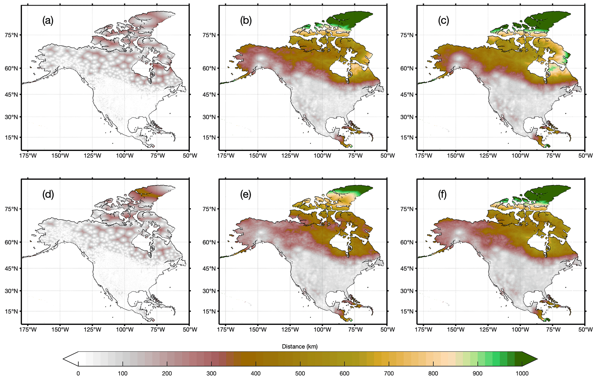
Figure 1The color of each 0.1∘ grid indicates the radius to find (a) 1, (b) 20, and (c) 30 neighboring stations for precipitation (a–c) and temperature (d–f).
Station observations are often subject to temporal discontinuities caused by missing values and short record lengths (Kemp et al., 1983). This study uses station precipitation and minimum and maximum temperature data from the Serially Complete Dataset for North America (SCDNA; Tang et al., 2020c), which is an open-access dataset on Zenodo (https://doi.org/10.5281/zenodo.3735533). Serially complete datasets improve the quality of spatial interpolation estimates compared to raw station observations with data gaps (Longman et al., 2020; Tang et al., 2021). Tmean and Trange are calculated from minimum and maximum temperature data. In SCDNA, raw measurements undergo strict quality control checks, and data gaps are filled by combining estimates from multiple strategies (including quantile mapping, spatial interpolation, machine learning, and multi-strategy merging). SCDNA uses reanalysis estimates as the auxiliary data to ensure temporal completeness in sparsely gauged regions. The production of SCDNA has nine steps: (1) matching reanalysis estimates and station data, (2) selecting qualified neighboring stations, (3) building empirical cumulative density functions (CDFs), (4) estimation based on 16 strategies for each day of the year, (5) independent validation, (6) merging estimates from the 16 strategies, (7) climatological bias correction, (8) evaluation of SCDNA, and (9) final quality control (Tang et al., 2020c). SCDNA covers the period from 1979 to 2018 and has 24 615 precipitation stations and 19 579 temperature stations. We select precipitation and temperature, because they are used in many hydrometeorological studies and are measured by a large number of meteorological stations, while other variables (e.g., humidity and wind speed) are only measured by a much smaller collection of stations.
Station-based gridded meteorological estimates usually rely on a certain number of neighboring stations surrounding the target grid cell. For most regions in CONUS, the search radius to find 20 or 30 neighboring stations (lower and upper limits for station-based gridded estimates in Sect. 3.1) is smaller than 100 km (Fig. 1). For the regions north of 50∘ N or south of 20∘ N, however, the search radius required to find 20 or 30 neighboring stations is much larger and even exceeds 1000 km in the Arctic Archipelago. The sparse station network at higher latitudes motivates our decision to optimally combine station data with reanalysis products.
The reanalysis products used in this study include the fifth generation of European Centre for Medium-Range Weather Forecasts (ECMWF) atmospheric reanalyses of the global climate (ERA5; Hersbach et al., 2020), the Modern-Era Retrospective analysis for Research and Applications, Version 2 (MERRA-2; Gelaro et al., 2017), and the Japanese 55-year reanalysis (JRA-55; Kobayashi et al., 2015). The three widely used products are chosen because of their high spatiotemporal resolutions and suitable time length. The spatial resolutions of ERA5, MERRA-2, and JRA-55 are , , and ∼ 55 km, respectively. Their start years are 1979, 1980, and 1958, respectively. Therefore, only ERA5 and JRA-55 are used for 1979 throughout this study. Although reanalysis models assimilate observations from various sources, they differ from station measurements in many aspects (Parker, 2016) and often contain large uncertainties as shown by assessment and multi-source merging studies (e.g., Donat et al., 2014; Lader et al., 2016; Beck et al., 2017, 2019; Tang et al., 2020b). The dependence of reanalysis estimates on station data may have a negative effect on the merging of reanalysis products (Sect. 3.2), because the reanalysis dataset which assimilates more station data could be given higher weight. The potential dependence, however, is not considered in this study because of the limited understanding of the dependence between reanalysis estimates and station observations. Moreover, none of the reanalysis datasets assimilate precipitation data from stations.
The elevation data are sourced from the 3 arcsec resolution Multi-Error-Removed Improved-Terrain digital elevation model (MERIT DEM; Yamazaki et al., 2017).
The estimate of a variable at a specific location and time step can be regarded as a random value following a probability distribution. The probability density functions (PDFs) of variables such as Tmean and Trange can be approximated using the normal distribution. Their value x for a target location and time step is expressed as
where μ is the mean value, and σ is the standard deviation. Probabilistic estimates of Tmean or Trange can be realized by sampling from this distribution. In a spatial meteorological dataset, the distribution parameters vary with space and time, and the spatial variability is related to the nature of variables and gridding (interpolation) methods. The performance of gridding methods is critical, because accurate estimation of μ can reduce systematic bias and smaller σ means narrower spread.
Precipitation is different from Tmean and Trange because it can be intermittent from local to synoptic scales, and its distribution is both highly skewed and bounded at zero. Following Papalexiou (2018) and Newman et al. (2019b), the CDF of precipitation can be expressed as below:
where FX(x) is the CDF for x≥0, FX|X > 0(x) is the CDF for x>0, and p0 is the probability of zero precipitation. The probability of precipitation (PoP) is 1−p0. The CDF FX|X > 0(x) is often approximated using the normal distribution after applying suitable transformation functions to observed precipitation. Clark and Slater (2006) perform the normal quantile transformation using an empirical CDF from station observations. Newman et al. (2015) apply a power-law transformation. Newman et al. (2019b) adopts the Box–Cox transformation, that is,
where λ is set to following Newman et al. (2019b) and Fortin et al. (2015). Equation (1) applies to x′, enabling the probabilistic estimation of precipitation. Unlike Newman et al. (2019b) that uses transformed precipitation throughout the production, this study only uses Box–Cox transformation when the assumption of normality is necessary (Sect. 3.2.4 and 3.3) to reduce the error introduced by the back transformation. The limitations and alternative choices of precipitation transformation are discussed in Sect. 5.2.
In summary, seven space- and time-varying parameters (μ and σ for three variables and PoP) should be obtained to realize probabilistic estimation. Our method to develop probabilistic meteorological estimates is summarized in Fig. 2a. We apply four main steps to produce EMDNA: (1) station-based regression estimates (Sect. 3.1); (2) the regridding, downscaling, bias correction, and merging of three reanalysis products (Sect. 3.2); (3) optimal interpolation-based merging of reanalysis and station-based regression outputs and the bias correction of the resulting precipitation estimates (Sect. 3.3); and (4) the production of probabilistic estimates in the form of spatial meteorological ensembles (Sect. 3.4).
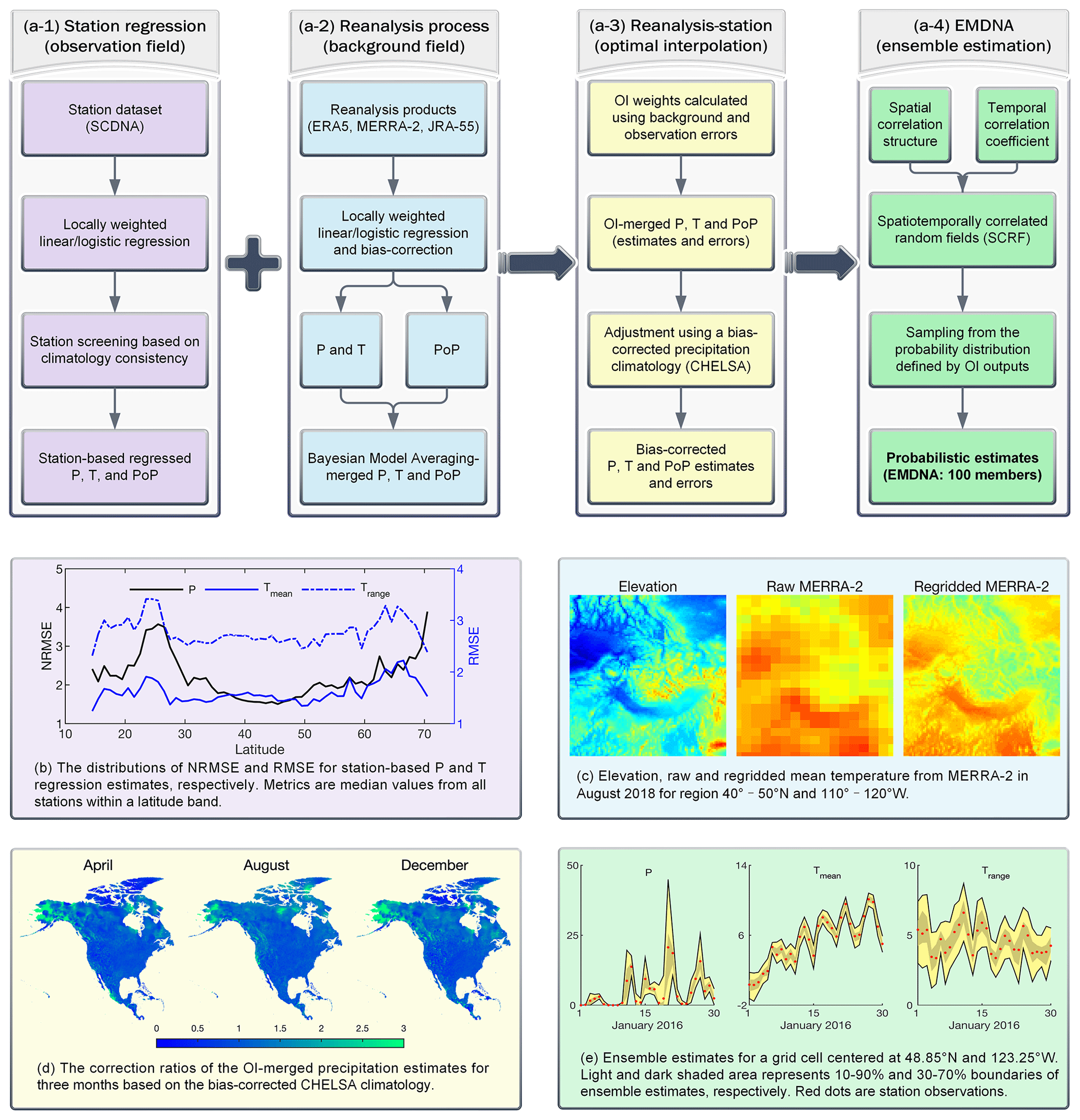
Figure 2(a) The flowchart outlining the main steps for producing EMDNA. P represents precipitation and T represents temperature. (b–e) demonstrate output examples from (a-1 to a-4), respectively. (b) Latitudinal distribution of the root mean square error (RMSE) for temperature and normalized RMSE (NRMSE) for precipitation (Sect. 3.1). (c) Example showing the mean temperature of MERRA-2 before and after regridding (Sect. 3.2). (d) The correction ratios calculated using precipitation climatology from the bias-corrected CHELSA (Sect. 3.3). (e) Example of the ensemble-based distributions of precipitation and temperature estimates from EMDNA (Sect. 3.4).
3.1 Regression estimates from station data
Clark and Slater (2006) and Newman et al. (2015, 2019b) use locally weighted linear regression and logistic regression to obtain gridded temperature and gridded precipitation estimates which are used as parameters in Eq. (1). However, for high-latitude regions in North America where stations are scarce (Fig. 1), such gridded estimates based only on station data could contain large uncertainties (Fig. 2b) due to the long distances needed to assemble a sufficient sample of stations to form the regressions. This study uses optimal interpolation (OI) to merge data from stations and reanalysis models. In this section, we only obtain regression estimates and their errors at the locations of stations, which are used as inputs to OI in Sect. 3.3.
3.1.1 Locally weighted linear regression
Daily precipitation amount, Tmean, and Trange are estimated for all stations based on the locally weighted linear regression (also known as the geographically weighted regression). Let xo be the station observation for variable X (precipitation, Tmean, and Trange), then the regression estimate for the target point and time step is obtained as below:
where Ai is the ith time-invariant topographic attribute (or predictor variables), β0 and βi are regression coefficients estimated using ordinary least squares, and ε is the residual (or error term). The topographic attributes are latitude, longitude, and elevation for Tmean and Trange. For precipitation, two more topographic attributes (west-east and south-north slopes) are used to account for windward and leeward slope precipitation differences. An isotropic Gaussian low-pass filter is used to smooth DEM before calculating slopes, which can reduce the influence of noise in a high-resolution DEM on the large-scale topographic effect of precipitation (Newman et al., 2015). Ideally, the scale of this smoothing reflects the scale at which terrain most directly influences precipitation or temperature spatial patterns; in this case the filter bandwidth is 180 km.
For a target station point, is obtained based on data from neighboring stations. Newman et al. (2015, 2019b) used 30 neighboring stations, without controlling for maximum station distance. The very low station density in high-latitude regions makes this configuration infeasible; hence, this study adopts a relatively flexible criterion for selecting neighboring stations: (1) finding at most 30 stations within a fixed search radius (400 km) and (2), if fewer than 20 stations are found, extending the search radius until 20 stations are found. The lower threshold is set to 20 to ensure that linear or logistic regression is robust. To incorporate local dependence, a tricube weighting function is used to calculate the weight wi,j between the target station i and the neighboring station j.
where di,j is the distance between i and j, and dmax depends on the maximum distance ( between i and all its neighboring stations. If is smaller than 100 km, dmax is set to 100 km; otherwise, dmax is set to km (Newman et al., 2015, 2019b). The cubic weight function is smoother compared to functions such as exponential functions and inverse distance functions, indicating that wi,j degrades with distance in a relatively slow way, which generally leads to smooth spatial variations of variables. The comparison of different weight functions could be a direction for future research. Regression coefficients are estimated by weighted least squares method (described in Appendix A).
We found that a small number of observation stations show a climatology that is notably statistically different from surrounding stations, which could cause an adverse effect on gridded estimates, particularly in sparsely gauged regions. Strategies to identify and exclude such stations are summarized in Appendix B.
3.1.2 Locally weighted logistic regression
PoP is estimated using the locally weighted logistic regression by fitting binary precipitation occurrence to topographic attributes:
The topographic attributes (Ai) are the same as those used by precipitation regression. Appendix A describes the method to estimate regression coefficients.
The errors of precipitation, temperature, and PoP estimates for all stations are calculated as the difference between regression estimates and station observations using the leave-one-out cross-validation procedure. The leave-one-out evaluation could be affected by the distributions of stations in some cases. For example, two stations with very close distance may both show very high accuracy in the leave-one-out evaluation (this is a problem for all station-based evaluation methods).
3.2 Regridding, correction, and merging of reanalysis datasets
The three reanalysis datasets (ERA5, MERRA-2, and JRA-55) have different spatial resolutions and contain systematic biases. In this section, we discuss steps taken to (1) regrid all reanalysis datasets to the resolution of EMDNA (0.1∘), (2) perform a correction to remove the systematic bias in original estimates, and (3) merge the three reanalysis datasets to produce a background field that improves over any individual reanalysis dataset, in support of the reanalysis–station merging described in Sect. 3.3.
3.2.1 Regridding of reanalysis datasets
Precipitation, Tmean, and Trange are regridded to 0.1∘ using locally weighted regression (Fig. 2c). Latitude, longitude, and elevation are used as predictor variables for simplicity. Precipitation or temperature lapse rates are implicitly considered by involving elevation in the regression. Raw reanalysis data from a 5×5 space window (i.e., 25 coarse-resolution grids) centered by the 0.1∘ target grid are used to perform the regression. Each grid is represented using its center point. This regridding method has been proven effective in previous studies (Xu et al., 2015; Duan and Li, 2016; Lu et al., 2020). Reanalysis estimates are also regressed to the locations of all stations to facilitate evaluation and weight estimation in the following steps, which can avoid the scale mismatch caused by using point-scale observations to evaluate 0.1∘ gridded estimates (Tang et al., 2018a).
We also tested other regridding methods such as the nearest neighbor, bilinear interpolation, and temperature lapse rate-based downscaling (Tang et al., 2018b). Results (not shown) indicated that their performance is generally inferior to the locally weighted regression with respect to several accuracy metrics.
3.2.2 Probability of precipitation estimation
Reanalysis precipitation can exhibit large biases in the number of wet days, because the models often generate many light precipitation events. To overcome this limitation, we designed two methods for determining the occurrence of reanalysis precipitation. The first is to use positive thresholds to determine precipitation occurrence. The threshold was estimated in two ways, namely by forcing reanalysis precipitation (1) to have the same number of wet days with station data or (2) to achieve the highest critical success index (CSI). Gridded thresholds can be obtained through interpolation and used to discriminate between precipitation events or non-events. However, this method can only obtain binary occurrence instead of continuous PoP between zero and one. The second method is based on univariate logistic regression. The amount of reanalysis precipitation is used as the predictor and the binary occurrence from station data is used as the predictand. The logistic regression is implemented for each reanalysis product in the same way as Sect. 3.1.2. The comparison between the threshold-based method and the logistic regression-based method shows the latter achieves higher accuracy. Therefore, we adopt the univariate logistic regression to estimate PoP for each reanalysis product in this study. The possible bias caused by station measurements is not considered.
3.2.3 Bias correction of reanalysis datasets
Considering reanalysis products contain systematic biases (Clark and Hay, 2004; Mooney et al., 2011; Beck et al., 2017; Tang et al., 2018b, 2020b), the linear scaling method (also known as multiplicative/additive correction factor; Teutschbein and Seibert, 2012) is used to correct reanalysis precipitation, Tmean, and Trange estimates. Reanalysis PoP is not corrected, because station information has been incorporated in the logistic regression. Let xr be the reanalysis estimate for variable X, then the corrected estimate for a target grid/point i is calculated as
where is the corrected reanalysis estimate, wi,j is the distance-based weight (Eq. 5), and and are the climatological mean for each month (e.g., all January months from 1979 to 2018) from station observations and reanalysis estimates for the jth neighboring station, respectively. The additive correction is used for Tmean and Trange, and the multiplicative correction is used for precipitation. The number of neighboring stations (m) is set to 10, which is smaller than that used for linear or logistic regression (Sect. 3.1) but should be enough for bias correction. The upper bound of is set to 10 to avoid overcorrection in some cases (Hempel et al., 2013).
Linear scaling can be performed at monthly (Arias-Hidalgo et al., 2013; Herrnegger et al., 2018; Willkofer et al., 2018) or daily (Vila et al., 2009; Habib et al., 2014) timescales by replacing and by the monthly mean (e.g., January in 1 year) or daily values. We compared the performance of corrections at different scales and found that monthly- or daily-scale corrections acquire more accurate estimates than the climatological correction. The climatological correction was adopted because (1) it preserves the absolute/relative trends better than daily or monthly corrections, and (2) the OI merging (Sect. 3.3) adjusts daily variability of estimates, which compensates for the limitation of climatological correction and makes daily- or monthly-scale correction unnecessary.
Quantile mapping is another widely used correction method (Wood et al., 2004; Cannon et al., 2015). We compared quantile mapping and linear scaling and found that they are similar in statistical accuracy, while quantile mapping achieves better probability distributions with much smaller Hellinger distance (Hellinger, 1909), which is a metric used to quantify the similarity between estimated and observed probability distributions. Nevertheless, quantile mapping could result in spatial smoothing of precipitation and temperature, particularly in high-latitude regions where stations are few. For example, Ellesmere Island, the northernmost island of the Canadian Arctic Archipelago, usually shows lower temperature in inland regions. However, quantile mapping will erase this gradient because reanalysis grids for this island are corrected based on stations on the coast. To ensure the authenticity of spatial distributions, quantile mapping is not used in this study.
3.2.4 Merging of reanalysis datasets
The three reanalysis products are merged using the Bayesian Model Averaging (BMA; Hoeting et al., 1999), which has proved to be effective in fusing multi-source datasets (Chen et al., 2015; Ma et al., 2018a, b). According to the law of total probability, the PDF of the BMA estimate can be written as
where E is the ensemble estimate, (r=1, 2, 3) is the bias-corrected estimate from three reanalysis products, is the predicted PDF based only on a specific reanalysis product, and is the posterior probability of reanalysis products given the station observation xo. The posterior probability can be identified as the fractional BMA weight wr with . BMA prediction can be written as the weighted sum of individual reanalysis products.
For Tmean and Trange, can be regarded as the normal distribution g(E|θr) defined by the parameter , where μr is the mean and is the variance (Duan and Phillips, 2010). For precipitation, if we apply Box–Cox transformation (Eq. 3) to positive events (> 0) and exclude zero events, its distribution is approximately normal, and can be represented using g(E|θr). Therefore, Eq. (8) can be written as
There are different approaches to infer wr and θr (Schepen and Wang, 2015). This study uses the log-likelihood function to estimate the parameters (Duan and Phillips, 2010; Chen et al., 2015; Ma et al., 2018b). The Expectation-Maximization algorithm (Raftery et al., 2005) can be applied to estimate parameters by maximizing the likelihood function. BMA weights are obtained for all stations and each month. Gridded weights are obtained using the inverse distance weighting interpolation.
Merging multiple datasets could affect the probability distributions and extreme characteristics of original datasets. This is not a major concern, because the merged reanalysis data are further adjusted by station data in OI merging (Sect. 3.3), which is a later step in the EMDNA process. Also, the probabilistic estimation of ensemble members (Sect. 3.4) has a large effect on estimates of extreme events.
Gridded errors of BMA-merged estimates are necessary to enable optimal interpolation (Sect. 3.3). The error estimation is realized using a two-layer cross-validation (Appendix C).
3.3 Optimal Interpolation-based merging of reanalysis and station data
3.3.1 Optimal Interpolation
OI has proven to be effective in merging multiple datasets (Sinclair and Pegram, 2005; Xie and Xiong, 2011) and has been applied in operational products such as CaPA (Mahfouf et al., 2007; Fortin et al., 2015) and the China Merged Precipitation Analysis (CMPA; Shen et al., 2014, 2018). Let xA be the OI analysis estimate. The OI analysis estimate (xA,i) for a target grid/point i and time step is obtained by adding an increment to the first guess of the background (xB,i). The increment is a weighted sum of the difference between observation and background values at neighboring stations.
where xO,j, xB,j, and wj are the observed value (subscript “O”), background value (subscript “B”), and weight for the jth neighboring station. Let xT be the true value, then the errors of observed and background values are and (or ), respectively. Assuming that (1) the observation and background errors are unbiased with an expectation of zero and (2) there is no correlation between background and observation errors, the weights that minimize the variance of the analysis errors can be obtained by solving
where w is the vector of ; R and B are m×m covariance matrices of εO,j and εB,j, respectively; and b is the m×1 vector of covariance between εB,i and εB,j. The background provided by reanalysis models assimilates observations in the production and is corrected in a way using station data (described in Sect. 3.2.3), which may affect the soundness of the second assumption. The effect of this slight violation, however, is rather small according to our results and previous studies (Xie and Xiong, 2011; Shen et al., 2014b, 2018).
Different approaches can be used to implement OI. For example, Fortin et al. (2015) used raw station observations as xO, and assumed that the background error is a function of error variance and correlation length, and the observation error is a function of error variance. The variances and correlation length are obtained by fitting a theoretical variogram using station observations. Xie and Xiong (2011) and Shen et al. (2014) use station-based gridded estimates as xO, and assume that the background error variance is a function of precipitation intensity, the cross-correlation of background errors is a function of distance, and the observation error variance is a function of precipitation intensity and gauge density. The parameters of those functions are estimated based on station data in densely gauged regions.
In this study, we adopt a novel design that calculates weights based on error estimation, a feature that is enabled by the probabilistic nature of the observational dataset. Regression estimates and their errors at station points (Sect. 3.1) are used as xO and εO, respectively. BMA-merged reanalysis estimates and their errors (Sect. 3.2) are used as xB and εB, respectively. We do not use gridded regression estimates because (1) will show weak variation if neighboring stations are replaced by neighboring grids, and (2) estimates of weights w could be unrealistic because of the spatial smoothing of interpolated regression errors. The advantages of this design are (1) weights and inputs closely match each other and (2) weights in sparsely gauged regions are not determined by parameters fitted in densely gauged regions. In regions with few stations, the errors of regression estimates could be larger than reanalysis estimates, resulting in a smaller contribution from regression estimates and a larger contribution from reanalysis estimates, which is the complementary effect we expect by involving reanalysis datasets in EMDNA.
The Box–Cox transformation is applied to precipitation estimates. Then, precipitation, PoP, Tmean, and Trange estimates provided by OI are used as μ and PoP required for generating meteorological ensembles.
3.3.2 Error of OI-merged estimates
Variance is a necessary parameter to enable ensemble estimation. The variance σ2 is represented using the mean squared error of OI estimates in this study. First, the error of OI analysis estimates () is obtained for all stations using the leave-one-out strategy. Then, the for the ith grid is obtained as a weighted sum of squared errors from neighboring stations:
where εA,j is the difference between the station observation and OI estimate at the jth neighboring station, and wi,j is the weight (Eq. 5).
3.3.3 Correction of precipitation undercatch
Considering station precipitation data usually contain measurement errors such as wind-induced undercatch particularly in high-latitude and mountainous regions, OI-merged precipitation is further adjusted using the Precipitation Bias Correction (PBCOR) dataset produced by Beck et al. (2020). The PBCOR climatology infers the long-term precipitation (without rain–snow separation) using a Budyko curve and streamflow observations collected from seven national and international sources, among which the Global Runoff Data Centre (GRDC), the U.S. Geological Survey (USGS), and the Water Survey of Canada Hydrometric Data (HYDAT) are data sources in North America. The streamflow stations are scarce in high-latitude regions and absent in Greenland. Three corrected datasets are provided, including WorldClim, version 2 (WorldClim V2; Fick and Hijmans, 2017), the Climate Hazards Group Precipitation Climatology, version 1 (CHPclim V1; Funk et al., 2015), and Climatologies at High Resolution for the Earth's Land Surface Areas, version 1.2 (CHELSA V1.2; Karger et al., 2017). The water balance-based method of Beck et al. (2020) considers all measurement errors (e.g., undercatch and wetting/evaporation loss) as a whole, and undercatch is the major error source in many regions. Note that the rain gauge catch error includes both undercatch and overcatch. The potential overcatch could be caused by splash of rain or blow snow collected on the wind shield (Folland, 1988; Zhang et al., 2019). Since overcatch is less common compared to undercatch and since the PBCOR dataset does not consider overcatch, the bias correction in this study only addresses the undercatch problem. Moreover, the water balance estimates of precipitation undercatch do not consider non-contributing areas of river basins (e.g., endorheic subcatchments), which are common in the Canadian Prairies and the northern Great Plains in the USA.
Although the three datasets show similar precipitation distributions after bias correction, CHELSA V1.2 is used because its period (1979–2013) is most similar to our study period (1979–2018). The correction of OI-merged precipitation is performed in two steps: (1) the ratio between bias-corrected CHELSA V1.2 and OI-merged long-term monthly precipitation is calculated at the 0.1∘ resolution during 1979–2013, and (2) daily OI-merged precipitation estimates during 1979–2018 are scaled using the corresponding monthly ratio map. The bias correction notably increases precipitation in northern Canada and Alaska (Fig. 2d), where precipitation undercatch is often significant due to the large proportion of snowfall. The uncertainties of gridded estimates are typically larger in high-latitude sparsely gauged regions and topographically elevated regions, which is partly related to the increased proportion of snowfall and hence larger gauge catch errors.
3.4 Ensemble generation
3.4.1 Spatiotemporally correlated random fields
Spatially correlated random fields (SCRFs) are used to sample from the probability distributions of precipitation and temperature. The SCRFs are produced using the following three steps. First, the spatial correlation structure is generated based on an exponential correlation function:
where di,j is the distance between grids i and j, and Clen is the spatial correlation length determined for each climatological month based on regression using station data for precipitation, Tmean, and Trange, separately. The spatial correlation structure is generated using the conditional distribution approach. Every point is conditioned to previously generated points which are determined using a nested simulation strategy to improve the calculation efficiency (Clark and Slater, 2006).
Second, the spatially correlated random field (Rt) for the tth time step is generated by sampling from the normal distribution with the mean value and standard deviation depending on the random numbers of previously generated grids (Clark and Slater, 2006).
Third, the SCRF is generated by incorporating spatial and temporal correlation relationships. Let ρTM and ρTR be the lag-1 autocorrelation for Tmean and Trange, respectively; ρCR be the cross-correlation between Trange and precipitation; and , , and be the SCRF for the (t−1)th time step for Tmean, Trange, and precipitation, respectively, then the SCRF for the tth time step following Newman et al. (2015) is written as
3.4.2 Probabilistic estimation
Probabilistic estimates are produced using the probability distribution N(μσ2) in Eq. (1) and R in Eq. (14). For Tmean and Trange, the SCRF (RTM and RTR) is directly used as the standard normal deviate (RX). The estimate (xe) for the ensemble member e is written as
For precipitation, an additional step is to judge whether an event occurs or not according to OI-merged PoP and the estimated probability from the SCRF. Let FN(x) be the CDF of the standard normal distribution, then FN(RPR) is the cumulative probability corresponding to the random number RPR. If FN(RPR) is larger than p0, then the scaled cumulative probability of precipitation (pcs) is calculated as
The probabilistic estimate for precipitation can be expressed as
3.5 Evaluation of probabilistic estimates
Independent stations that are not used in SCDNA are used to evaluate EMDNA, because the leave-one-out strategy is too time-consuming to evaluate probabilistic estimates. GHCN-D (Global Historical Climate Network Daily) stations with precipitation or temperature records less than 8 years are extracted, because SCDNA restricts attention to stations with at least 8-year records. In total, 15 018 precipitation stations and 2455 temperature stations are available for independent testing.
The Brier skill score (BSS; Brier, 1950) is used to evaluate probabilistic precipitation estimates. The continuous ranked probability skill score (CRPSS) is used to evaluate probabilistic temperature estimates. Their definitions are described in Appendix D.
Furthermore, the reliability and discrimination diagrams are used to assess the behavior of probabilistic precipitation estimates. The reliability diagram shows the conditional probability of an observed event (precipitation above a threshold) given the probability of probabilistic precipitation estimates. In a reliability diagram, a perfect match has all points located on the 1–1 line. The discrimination diagram shows the PDF of probabilistic precipitation estimates for different observed categories. For precipitation, two categories are defined: events or non-events, i.e., observed precipitation above or below a threshold. The difference between PDF curves of events or non-events represents the degree of discrimination. Larger discrimination is preferred. The PDF for non-event (event) should be maximized at the probability of zero (one).
4.1 Comparison between raw and merged reanalysis estimates
The three raw reanalysis estimates are regridded, corrected for bias, and merged. In this section, we directly compare raw and BMA-merged estimates. The evaluation is performed for all stations using the two-layer cross-validation strategy. The correlation coefficient (CC), root mean square error (RMSE), and normalized RMSE (NRMSE) are used as evaluation metrics. RMSE is sued for Tmean, and NRMSE is used for precipitation and Trange to remove patterns caused by climatology.
For precipitation, the three reanalysis products show the highest CC in CONUS and the lowest CC in Mexico (Fig. 3). The slight spatial discontinuity of CC along the Canada–USA border and the USA–Mexico border (Fig. 3 and 6) is caused by the inconsistent reporting time of stations. Daily precipitation from reanalysis products is accumulated from 00:00 to 24:00 UTC, while stations from different countries or regions usually have different UTC accumulation periods (Beck et al., 2019; Tang et al., 2020a). NRMSE is higher in central CONUS and Mexico compared to other regions. Overall, ERA5 outperforms MERRA-2 followed by JRA-55.
BMA-merged precipitation estimates show higher accuracy than all reanalysis products (Fig. 3). The improvement of CC and NRMSE is the most evident in the Rocky Mountains, while for MERRA-2 the improvement is also obvious in central CONUS. ERA5 is the closest to BMA estimates concerning CC and NRMSE. The improvement of BMA estimates against ERA5 is more prominent in the high-latitude regions. Specifically, the mean CC increases by 0.05 and 0.07 in regions south of and north of 55∘ N, respectively. The corresponding decrease of mean NRMSE is 0.15 and 0.21, respectively.
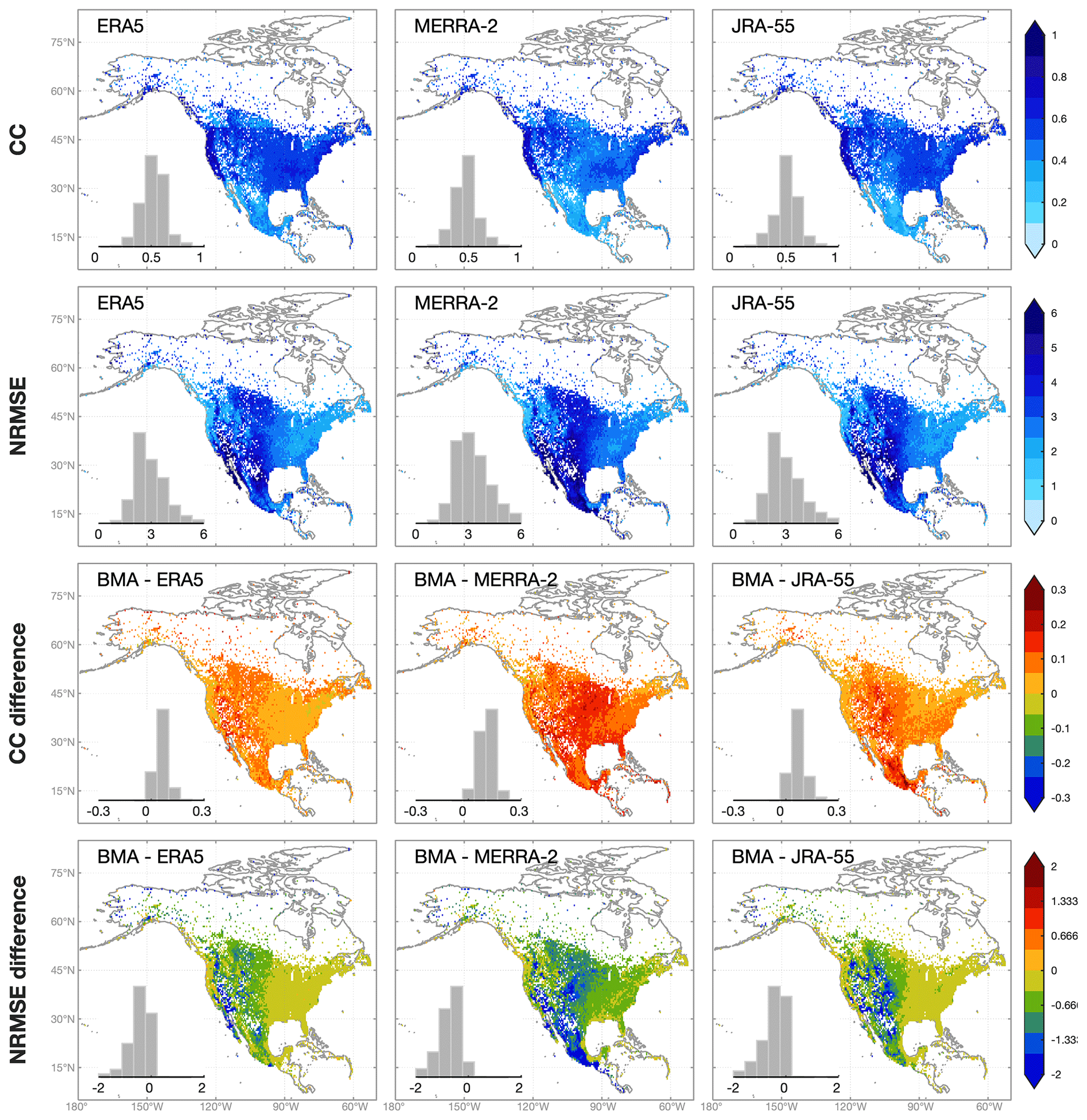
Figure 3The spatial distributions and histograms of CC (the first row) and NRMSE (the second row) based on raw reanalysis precipitation estimates (ERA5, MERRA-2, and JRA-55). The improvement of BMA-merged estimates against raw reanalysis estimates is shown in the third and fourth rows. The maps are at the 0.5∘ resolution, and the value of each 0.5∘ grid point is the median metric of all stations located within the grid.
The CC of reanalysis Tmean estimates is close to one in most regions of North America (Fig. 4) and still above 0.9 in Mexico where the CC is the lowest. According to RMSE, Tmean estimates have the largest error in western North America, because coarse-resolution raw reanalysis estimates cannot reproduce the variability of temperature caused by elevation variations. The rank of three reanalysis products for Tmean is the same as that for precipitation with ERA5 being the best one. BMA estimates show higher CC than reanalysis products particularly in Mexico, while the improvement of RMSE is the most notable in the Rocky Mountains. For a few stations, the RMSE of BMA estimates is slightly worse than raw reanalysis estimates (Fig. 4) because the downscaling of reanalysis temperature could occasionally magnify the error in low-altitude regions (Tang et al., 2018b).
For Trange, BMA estimates show much larger improvement than Tmean, while the differences of CC and NRMSE are relatively evenly distributed (Fig. 5). The improvement of BMA estimates against JRA-55 estimates is especially large. In general, BMA is effective in improving the accuracy of reanalysis precipitation and temperature estimates.
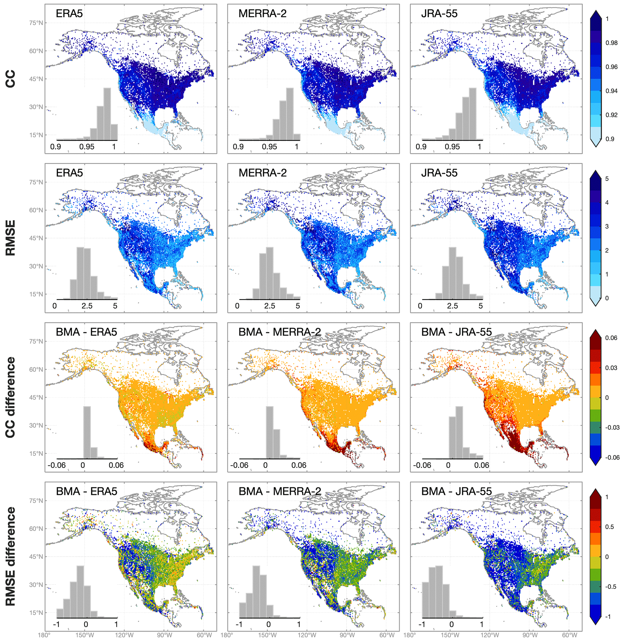
Figure 4Same as Fig. 3 but for mean temperature.
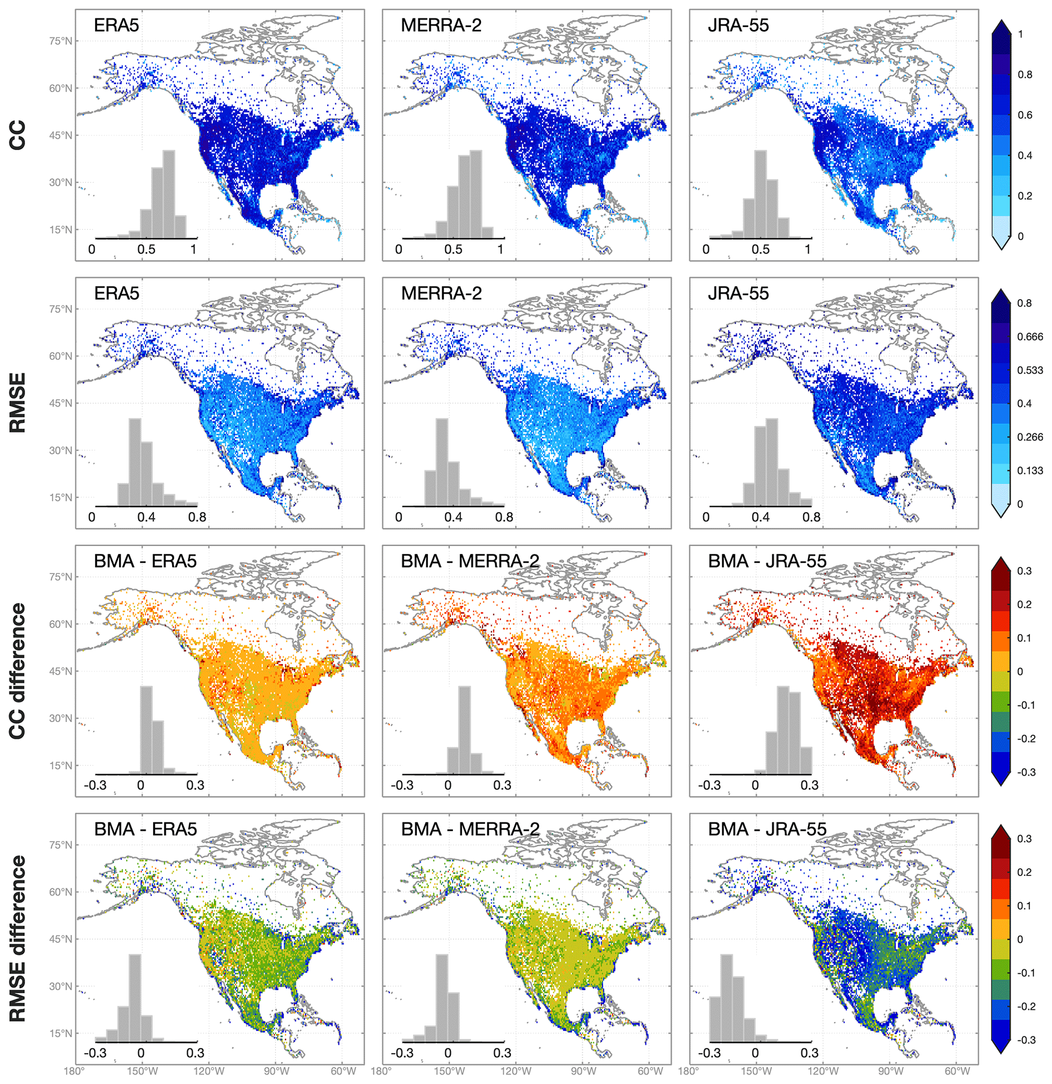
Figure 5Same as Fig. 3 but for daily temperature range.
4.2 The performance of optimal interpolation
Optimal interpolation is used to combine station-based estimates with reanalysis estimates. The performance of OI-merged precipitation and temperature estimates is compared to the background (BMA-merged reanalysis estimates; Fig. 6) and observation (station-based regression estimates; Fig. 7) inputs. To better show the spatial variations of the improvement of OI estimates, RMSE for precipitation and Trange is normalized using the mean value (termed as NRMSE), while Tmean is evaluated using RMSE.
Overall, OI estimates are more accurate than merged reanalysis or station regression estimates for all variables across North America. Comparing OI estimates to reanalysis estimates, for precipitation, Tmean, and Trange, the mean CC is improved by 0.24, 0.02, and 0.15, respectively, and the mean RMSE is reduced by 1.88 mm d−1, 0.52∘, and 0.87∘, respectively. The improvement of OI estimates against station estimates is smaller with the mean CC increasing by 0.06, 0.01, and 0.05, and the mean RMSE decreasing by 0.56 mm d−1, 0.18∘, and 0.29∘ for precipitation, Tmean, and Trange, respectively.
OI can utilize the complementarity between station and reanalysis estimates. For example, according to CC, the improvement of OI estimates against reanalysis estimates is larger in the eastern than the western CONUS, while the improvement against station estimates is larger in western than eastern CONUS. This means that although station estimates generally show higher accuracy than reanalysis estimates, station estimates face more severe quality degradation in mountainous regions. Moreover, the latitudinal curves of CC and NRMSE in Figs. 6 and 7 indicate that the improvement of OI estimates against reanalysis estimates decreases as the latitude increases from southern CONUS to northern Canada, while the improvement against station estimates shows a reverse trend.
For Tmean, the CC improvement for OI estimates is the largest in Mexico and decreases from low to high latitudes, while based on RMSE, the improvement increases with latitude. For Trange, the latitudinal variation exhibits a similar pattern with precipitation for regions north of 50∘ N, with larger (smaller) improvement in higher latitudes against station (reanalysis) estimates. For regions south of 50∘ N, the improvement of CC and NRMSE against station estimates shows different trends.
Station-based estimates often have lower accuracy in regions with scarce stations (i.e., high-latitude North America), while reanalysis estimates could have less dependence on station densities due to the compensation of physically based models. Therefore, OI merging is particularly useful in sparsely gauged regions.
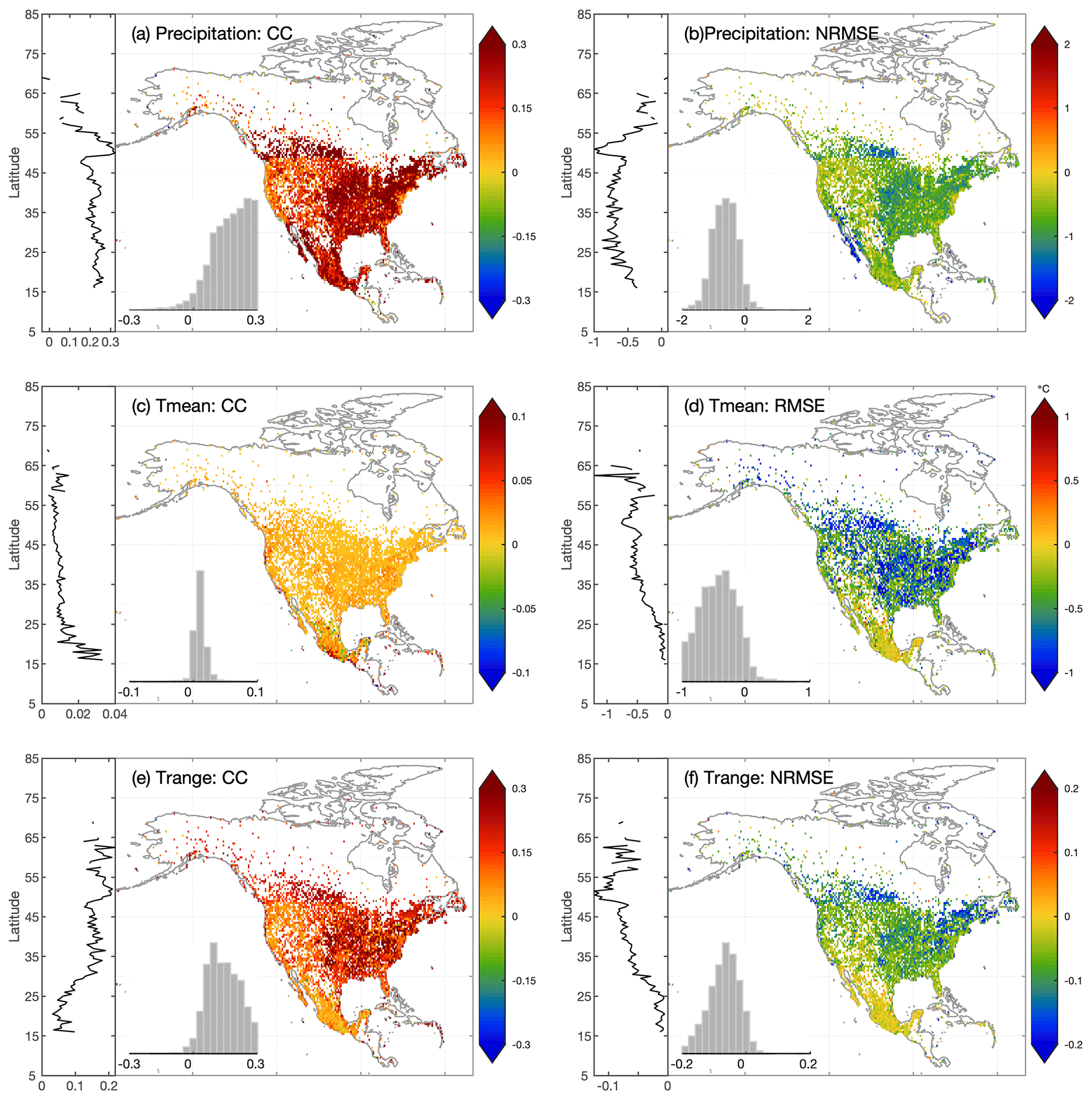
Figure 6The differences of (a) CC and (b) NRMSE (normalized RMSE) between OI-merged precipitation estimates and BMA-merged reanalysis precipitation estimates. The latitudinal distributions of metrics are attached on the left side, showing the median value for 0.5∘ latitude bands. Panels (c–d) are the same as (a–b) but for mean temperature, and RMSE is not normalized. Panels (e–f) are the same as (a–b) but for daily temperature range.
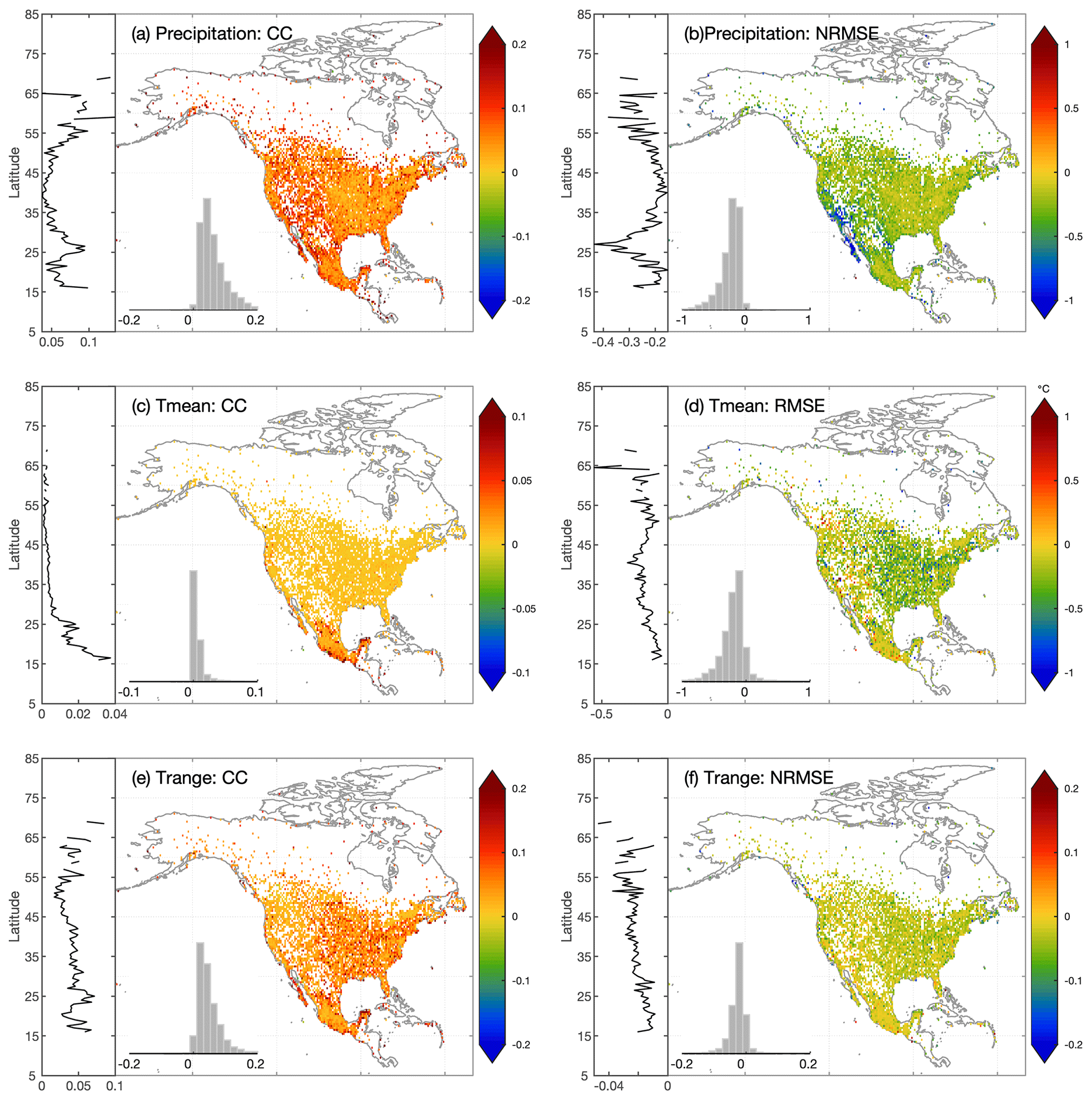
Figure 7Similar with Fig. 6, but the differences are between OI-merged precipitation estimates and station-based regression precipitation estimates.
4.3 Evaluation of probabilistic estimates
The distributions of the OI and ensemble precipitation, Tmean, and Trange estimates in June 2016 are shown in Fig. 8. Compared with OI precipitation estimates, ensemble precipitation estimates show generally consistent but less smooth distributions because of the relatively short spatial correlation length in the warm season. For Tmean and Trange, OI and ensemble estimates show very similar spatial distributions. Precipitation shows the largest standard deviation, while Tmean shows the smallest, because the standard deviation is determined by the errors of OI estimates. The PoP from station observations and ensemble estimates is compared based on stations with at least 5-year-long records from 1979 to 2018 (Fig. 9). The comparison cannot represent climatological PoP (Newman et al., 2019b) due to short time length of independent stations (Sect. 3.5). Overall, EMDNA estimates show similar PoP distributions with station observations. The PoP in Canada is slightly overestimated because (1) the quality of EMDNA is lower in regions with fewer stations, and (2) point-scale station observations could underestimate the PoP at a larger scale (e.g., 0.1∘ grids) as shown by Tang et al. (2018a).
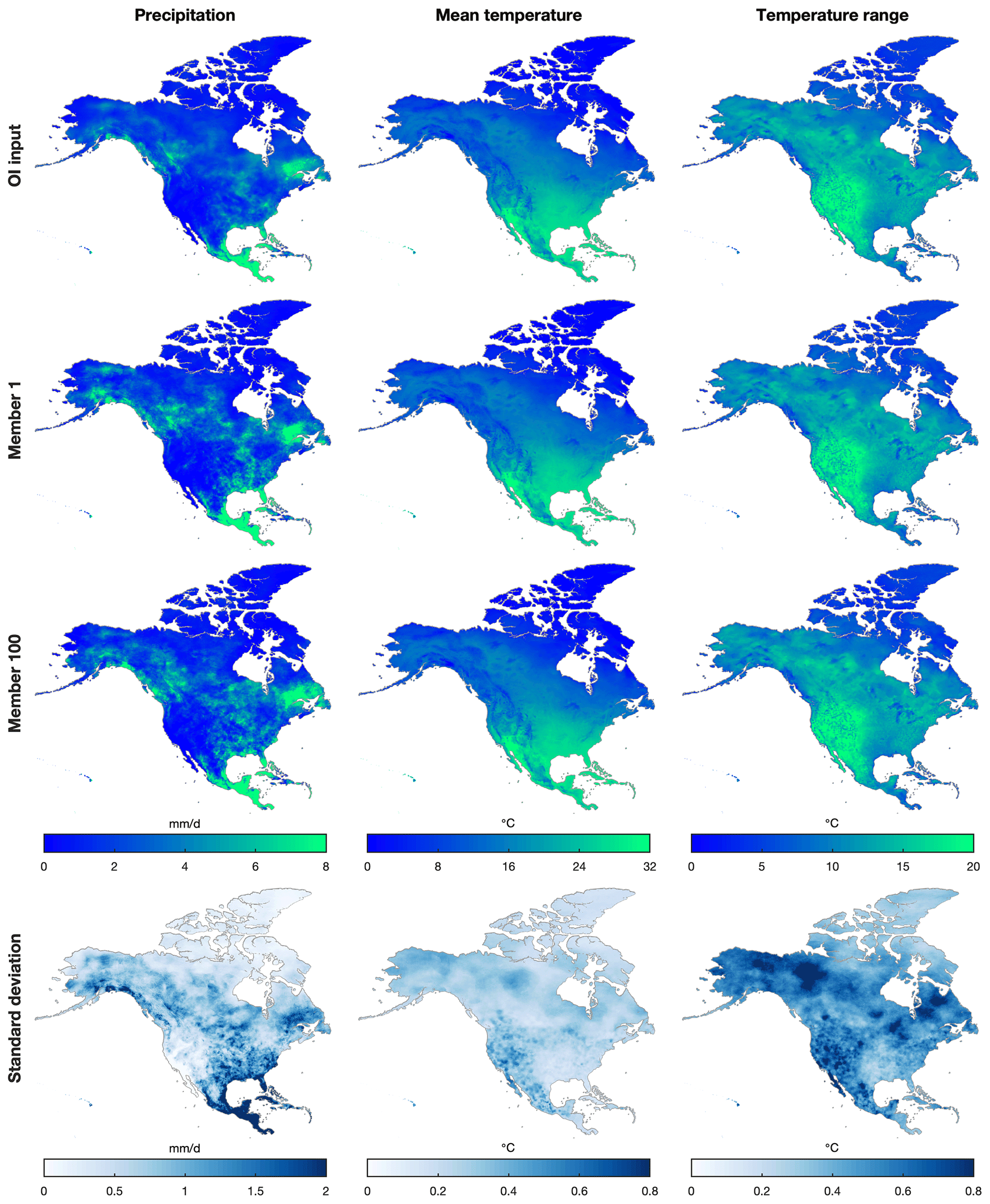
Figure 8The distributions of average values from precipitation (the first column), mean daily temperature (the second column), and daily temperature range (the third column) averaged over the period 1–30 June 2016. The first to third rows represent estimates from OI-merged inputs, ensemble member 1, and ensemble member 100. The fourth row represents the standard deviation of all the 100 members for 1 month (June 2016).
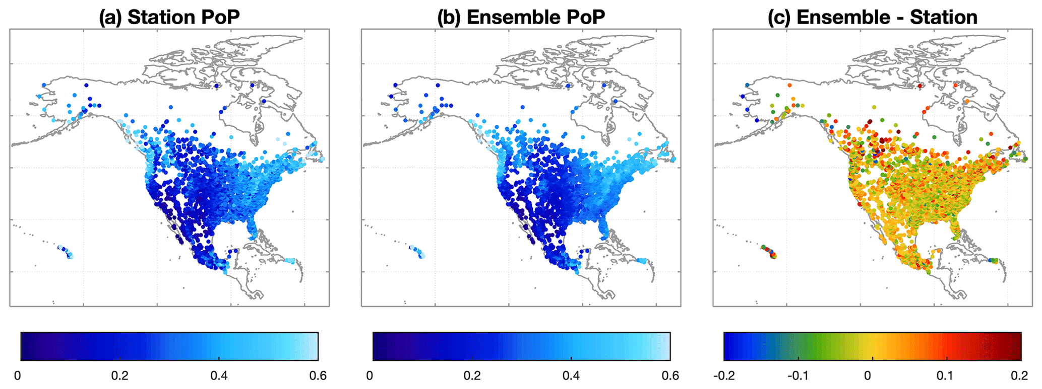
Figure 9The probability of precipitation (PoP) from (a) station observations and (b) concurrent EMDNA ensemble estimates with their differences shown in (c). Stations with at least 5-year-long records from 1979 to 2018 are involved in the comparison.
The discrimination diagram (Fig. 10) shows that ensemble precipitation assigns the highest occurrence frequency at the lowest estimated probability for non-precipitation events, and the performance becomes better as the threshold increases from 0 to 50 mm. For precipitation events, ensemble estimates show the highest frequency at the highest estimated probability for the thresholds of 0, 10, and 25 mm, while as the threshold increases, the frequency curve becomes skewed to the lower estimated probability. This problem is also seen in Clark and Slater (2006) and Newman et al. (2015). Ensemble precipitation shows good reliability for all precipitation thresholds with the points located at or close to the 1–1 line (Fig. 10). At low and high estimated probabilities of occurrence, ensemble precipitation shows slight wet bias. The reliability performance does not show clear dependence with thresholds.
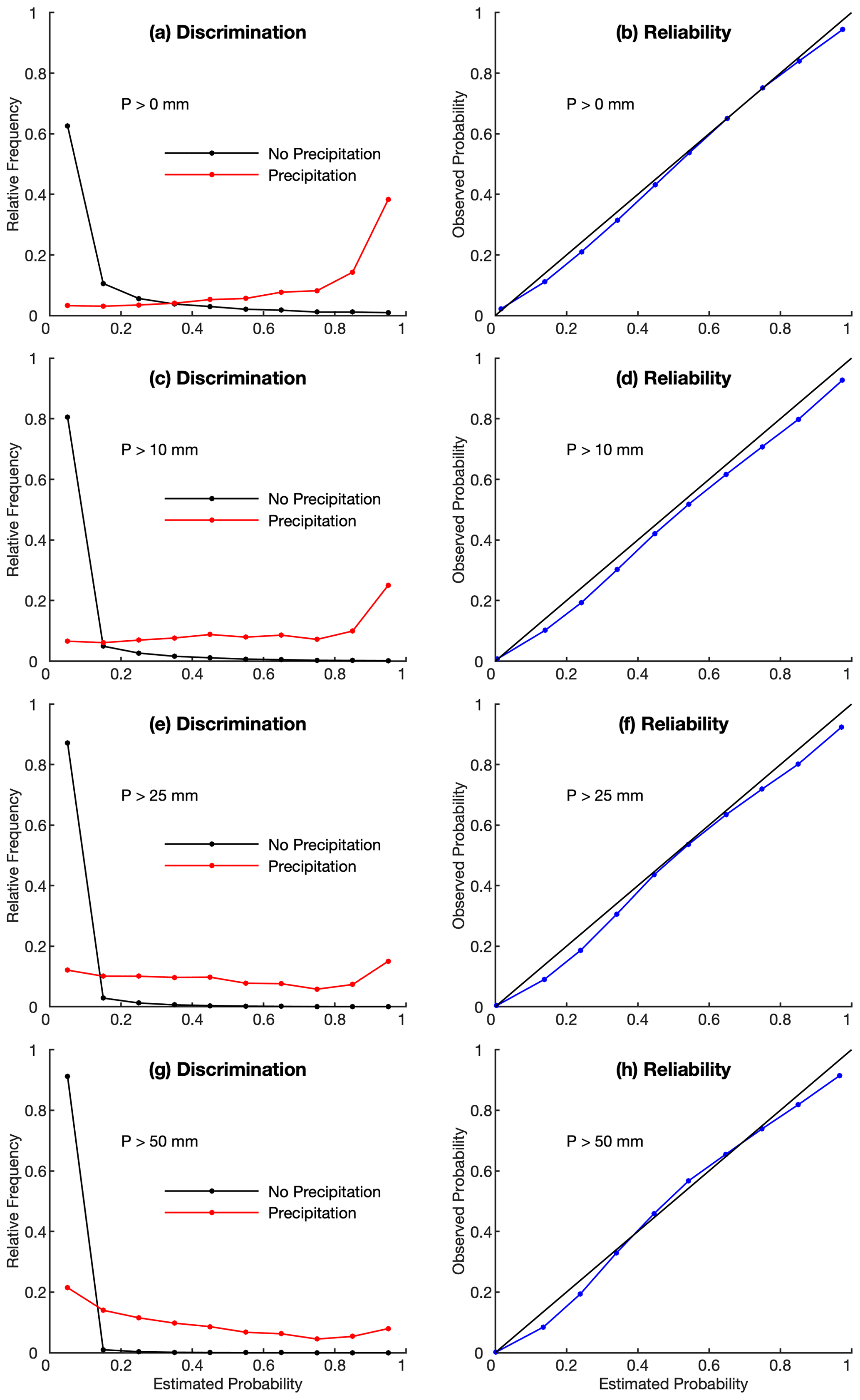
Figure 10The discrimination and reliability diagrams based on ensemble precipitation estimates. Four rain–no-rain thresholds (0, 10, 25, 50 mm) are used.
The BSS for precipitation and CRPSS for Tmean and Trange are shown in Fig. 11. In most cases, ensemble precipitation shows the highest frequency when BSS is above 0.5. As the precipitation threshold increases, the BSS values decrease. The median BSS values are 0.62, 0.54, and 0.46 for the thresholds of 0, 10, and 20 mm d−1, respectively. We note that a small number of cases show BSS values smaller than zero, indicating that the ensemble estimated probability is worse than climatological probability. A low BSS value usually occurs in regions where precipitation is hard to estimate (e.g., Rocky Mountains), resulting in inaccurate parameters of Eq. (1).
The BSS for all thresholds shows a clear increasing trend from 1979 to 2018 (Fig. 11b), because the observed precipitation samples from SCDNA increase during this period (Fig. 2 in Tang et al., 2020c). The increasing trend of BSS is particularly prominent from 2003 to 2009, during which precipitation samples in the USA experience the greatest increase (Tang et al., 2020c). The results show that although infilled station data contribute to higher station densities, observation samples still have a significant effect on gridded data estimation.
Tmean shows high CRPSS for most cases with the frequency peak occurring at ∼ 0.8. The CRPSS of Trange is much lower with the peak occurring at ∼ 0.6. The median CRPSS for Tmean and Trange is 0.74 and 0.51, respectively. Trange shows lower CRPSS probably because the bias direction (i.e., overestimation or underestimation) of daily minimum and maximum temperature could be different, resulting in the larger bias of Trange than Tmean. Analyses show that among stations with negative CRPSS, most are located in Mexico due to the degraded quality of temperature estimates (Sect. 4.1 and 4.2). The long-term variation of CRPSS is not shown, because independent temperature stations are insufficient to support validation between 1986 and 2010.
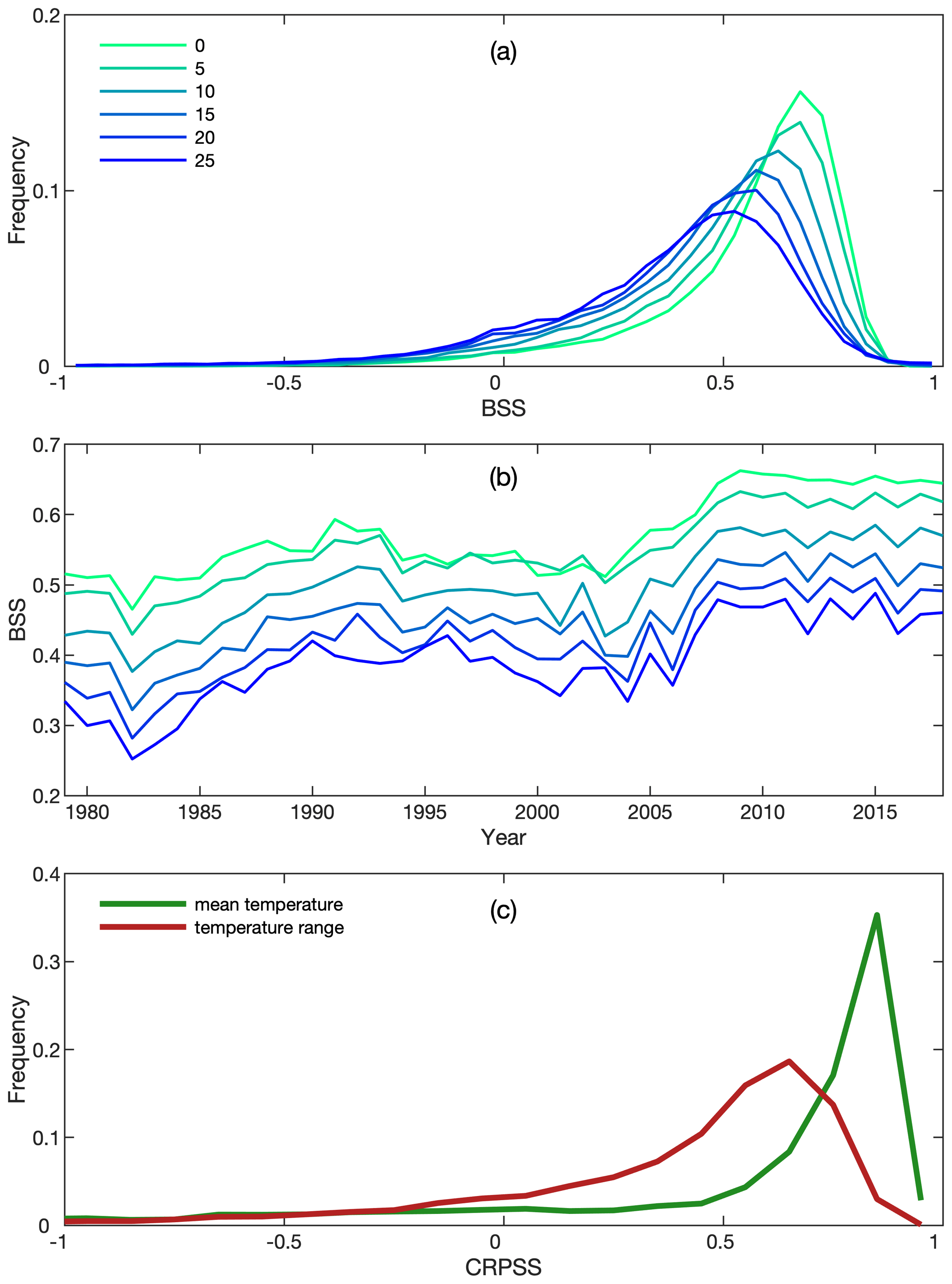
Figure 11(a) The frequency distributions of the Brier skill score (BSS) for precipitation corresponding to rain–no-rain thresholds from 0 to 25 mm d−1. (b) The distributions of BSS for precipitation from 1979 to 2018. For each year, the median value of all stations is used. (c) The frequency distributions of the continuous ranked probability skill score (CRPSS) for daily mean temperature and daily temperature range.
This study presents the framework for producing an ensemble precipitation and temperature dataset over North America. Although we have tested multiple choices of methods (Sect. 3) and overall the product shows good performance (Sect. 4), the methodology still has limitations that need to be improved through continued efforts.
5.1 Implementation of OI
OI is used to merge reanalysis outputs and station data. To implement OI-based merging, a critical step is to estimate the weights. Previous studies usually adopt empirical error or variogram functions and fit the parameters using station observations (e.g., CaPA, Fortin et al., 2015, and CMPA, Shen et al., 2018); then the parameters are constant for the whole study area in the actual application.
In this study, we proposed a novel design, which uses station-based regression estimates as the observation field and calculates weights by directly solving the weight functions based on observation and background errors. Compared with methods that use station data as the observation field, our method is characterized by inferior estimation of the observation field but realistic estimation of weights. The close linkage between the observation field and the weights could benefit OI estimates, but comparing different OI implementations is still meaningful and necessary considering that OI has been widely used and is the core algorithm of some operational products.
Furthermore, regression estimates show worse performance in regions with fewer stations. More advanced interpolation methods that can utilize climatology information and comprehensively consider topographic and atmospheric conditions (Daly et al., 2008; Newman et al., 2019b; Newman and Clark, 2020) should be examined in future studies.
5.2 Probabilistic estimation
Power transformations (e.g., Box–Cox and root or cubic square) with fixed parameters have proven to be useful in precipitation estimation and dataset production (Fortin et al., 2015, 2018; Cornes et al., 2018; Khedhaouiria et al., 2020; Newman et al., 2020). The Box–Cox transformation with a constant parameter is applied following Fortin et al. (2015) and Newman et al. (2019b, 2020). A fixed parameter, however, cannot ensure that transformed precipitation is normally distributed everywhere as is desirable. We tested a series of additional parametric and non-parametric transformations based on power functions, logarithmic functions, or a mix of both and optimized the parametric transformation functions (including Box–Cox) for every grid by minimizing the objective function which is the sum of squared L-skewness and L-kurtosis (Papalexiou and Koutsoyiannis, 2013). Theoretically, compared to a Box–Cox transformation with a fixed parameter, the optimized functions can obtain precipitation series closer to the normal distribution which should benefit probabilistic estimation, while the evaluation results show that the Box–Cox transformation with a fixed parameter is better at probabilistic estimation than optimized functions. We suggest there are three reasons for this: (1) the standard deviation in Eq. (1) is obtained by interpolating OI errors (Sect. 3.2.2) from neighboring stations, whereas the optimized transformation parameters could be different at those stations; (2) zero precipitation is excluded during optimization to avoid invalid transformation or optimization, which reduces the number of stations for every time step and thus degrades the quality of the spatial interpolation; and (3) the errors caused by back transformation could be large if the optimized transformation is too powerful. More efforts are needed to resolve this problem.
There are other potential directions for improvement. For example, SCRF is generated from Gaussian distributions, while other choices such as copulas functions (Papalexiou and Serinaldi, 2020) show potential in probabilistic estimation. The spatial correlation length is constant for the whole study area following Newman et al. (2015, 2019b), which may introduce uncertainties for a large domain. Overall, studies related to the production of ensemble meteorological datasets are still insufficient, particularly for large areas. More studies are needed to clarify the critical issues in large-scale probabilistic estimation and explore the effect of parameter/method choices on probabilistic estimates.
5.3 Alternate data sources
The quality of source data (station observations and reanalysis models) primarily determines the quality of output datasets. The density of stations has a critical effect on the accuracy of the observation field and probabilistic estimates. While SCDNA collects data from multiple datasets, efforts are ongoing to expand the database by involving station sources such as provincial station networks in Canada.
For reanalysis products, ERA5, MERRA-2, and JRA-55 are regridded using locally weighted linear regression to meet the target resolution. There are some choices for future improvement, such as (1) adopting and/or developing better downscaling methods or (2) utilizing outputs from high-resolution reanalysis products or forecasting models such as ERA5-Land (Muñoz-Sabater et al., 2021) or the Arctic System Reanalysis (Bromwich et al., 2018). Moreover, including other data sources such as satellite and weather radar estimates is also an opportunity for regions with adequate sample coverage.
5.4 Precipitation undercatch
Although station precipitation observations are used as the reference in this study, these values are subject to measurement errors such as wetting loss, wind-induced undercatch, and trace precipitation. Station temperature measurements also contain errors due to microclimate and sensor design, which is generally small and not discussed here. The undercatch of precipitation is particularly severe in high latitudes and mountains due to the stronger wind and frequent snowfall (Sevruk, 1984; Goodison et al., 1998; Nešpor and Sevruk, 1999; Yang et al., 2005; Scaff et al., 2015; Kochendorfer et al., 2018). For example, underestimation of precipitation could be larger than 100 % in Alaska (Yang et al., 1998). Bias correction of station precipitation data should consider many factors such as gauge types, precipitation phase, and environmental conditions, which would be very complicated when a large number of sparsely distributed stations are involved over the whole of North America.
The undercatch correction used in this study relies on bias-corrected precipitation climatology produced by Beck et al. (2020), which infers the long-term precipitation using a Budyko curve and streamflow observations. The bias-corrected precipitation climatology, however, is less accurate in northern Canada where streamflow stations are few (Beck et al., 2020). The streamflow data used by the bias-corrected climatology also contain uncertainties (Hamilton and Moore, 2012; Kiang et al., 2018) related to factors such as streamflow derivation methods (e.g., rate curves) and measurement instruments. In addition, this correction method aims to constrain the total precipitation amount and cannot distinguish between rainfall and snowfall which show different gauge catch performance. Data users can realize rain–snow classification using approaches such as temperature threshold-based methods and reanalysis model-based snowfall proportion. Moreover, as mentioned earlier, the water balance estimates of precipitation undercatch do not consider noncontributing areas of river basins. Whilst various undercatch correction methods (e.g., Fuchs et al., 2001; Beck et al., 2020; Newman et al., 2020) exist, further studies are needed to compare these solutions, considering their effectiveness and availability of input data in a large domain.
The EMDNA dataset is available at https://doi.org/10.20383/101.0275 (Tang et al., 2020a) in netCDF format. Individual ensemble member; ensemble mean; and ensemble spread of precipitation, Tmean, and Trange are provided. Since the 100 members are equally plausible, users can download fewer members if the storage space and processing time are limited. The deterministic OI estimates of precipitation, PoP, Tmean, and Trange produced in this study are also available in netCDF format. The high-quality OI estimates merge reanalysis and station data, which can be useful for applications that do not need ensemble forcings. The data sizes are 3.35 TB for the probabilistic part and 40.84 GB for the deterministic part.
The ensemble mean of the 100 members for Tmean and Trange is similar to deterministic OI estimates. For precipitation, the ensemble mean is slightly higher than deterministic OI estimates due to the back transformation. We recommend that users select the deterministic dataset instead of the ensemble mean if their applications do not involve uncertainty characterization.
A teaser dataset of probabilistic estimates is provided to facilitate easy preview of EMDNA without downloading the entire dataset. The teaser dataset covers the region from −116.8 to −115.2∘ W and 50.7 to 51.9∘ N, the time from 2014 to 2015, and the ensemble members from 1 to 25. The total data size is smaller than 30 MB. See Appendix E for a brief introduction.
Ensemble meteorological datasets are of great value to hydrological and meteorological studies. Given the lack of a historical ensemble dataset for the entire North America, this study develops EMDNA by integrating multi-source information to overcome the limitation of sparse stations in high-latitude regions. EMDNA contains precipitation, Tmean, and Trange estimates at 0.1∘ spatial resolution and daily temporal resolution from 1979 to 2018 with 100 members. Multiple methodological choices are examined when determining critical steps in the production of EMDNA. The ultimate framework is composed of four main steps: (1) generating station-based interpolation estimates from SCDNA using locally weighted linear or logistic regression; (2) regridding, correction, and merging of reanalysis products (ERA5, MERRA-2, and JRA-55); (3) merging station–reanalysis estimates using OI based on a novel method of OI weight calculation and correcting precipitation undercatch using the PBCOR dataset; and (4) generating ensemble estimates by sampling from the estimated probability distributions with the perturbations provided by SCRF.
The performance of each step is comprehensively evaluated using multiple methods. The results show that the design of the framework is effective. In short, we find that (1) station-based interpolation estimates are less accurate in regions with sparse stations (e.g., high latitudes) and complex terrain; (2) BMA-merged reanalysis estimates show notable improvement against raw reanalysis estimates, particularly for precipitation and Trange and over high-latitude regions; (3) OI achieves more accurate estimates than interpolation and reanalysis estimates from (1) and (2), respectively, and the complementary effect between reanalysis and interpolation estimates contributes to the large improvement of OI estimates in sparsely gauged regions; and (4) ensemble precipitation estimates show good discrimination and reliability performance for all thresholds, and the BSS values for ensemble precipitation and CRPSS values for ensemble Tmean and Trange are high in most cases. BSS values of ensemble precipitation increase from 1979 to 2018 due to the increase in the number of stations. Overall, EMDNA (version 1) will be useful for many applications in North America such as regional or continental hydrological modeling. Meanwhile, we recognize that the current framework is not perfect and have provided suggestions for the future directions for large-scale ensemble estimation of meteorological variables. Continuing efforts from the community are needed to promote the development of probabilistic estimation methods and datasets. Development of datasets at higher resolutions (e.g., 1 km and hourly) is also an important direction to enable more sophisticated hydrometeorological studies (e.g., Sampson et al., 2020).
The coefficients for locally weighted linear regression are estimated using weighted least squares. Given a station i with m neighboring stations, let be the attribute matrix, let be the station observations from neighboring stations, and let be the weight vector with distance-based weights computed from Eq. (5). The regression coefficients ) for Eq. (4) are estimated from the weighted normal equation as
where the m×m weight matrix W=Imwi is a diagonal matrix obtained by multiplying the m×m identity matrix Im with the weight vector wi.
The regression coefficients for logistic regression (Eq. 6) are estimated iteratively as
where P0 is a vector of binary precipitation occurrence for neighboring stations, π is the vector of estimated PoP for neighboring stations, and V is the diagonal variance matrix for PoP. The regression coefficients βold are initialized as a vector of ones.
To exclude climatologically anomalous stations, for temperature (Tmean or Trange), we calculate (1) the absolute difference in the climatological mean between the target station and the average value of its 10 neighboring stations (referred to as Diff-1) and (2) the absolute difference in the climatological mean between station observation and regression estimates (referred to as Diff-2). A temperature station will be excluded if its Diff-1 is larger than the 95 % percentile and its Diff-2 larger than the 99 % percentile of all stations simultaneously. The threshold of percentiles for Diff-1 is lower to better identify some climatologically anomalous stations.
For precipitation, the ratio (Ratio-1 and Ratio-2) is obtained in the same way with the Diff-1 and Diff-2 of temperature. A two-tailed check is used for precipitation compared with the one-tailed check for temperature. A precipitation station will be excluded if its Ratio-1 is larger (or smaller) than the 99.9 % (1 %) percentile and its Ratio-2 larger (or smaller) than the 99.9 % (1 %) percentile simultaneously. This check has more tolerance for heavy precipitation but tries to exclude more extremely dry stations.
As a result, ∼ 1.5 % precipitation and temperature stations are rejected, after which algorithms described in Sect. 3.1.1 and 3.1.2 are rerun. Stations can be anomalous because they are badly operated or simply because they are unique in terms of topography or climate. The usage of Diff-2 or Ratio-2 is helpful to avoid excluding unique stations. But for cases where the regression is ineffective, the unique stations can still be wrongly excluded. Although the effect on final estimates could be rather small, better strategies could be used in future studies.
The errors of BMA-merged estimates are first estimated for all stations and then interpolated to grids. Considering station observations cannot be used to evaluate merged estimates once they are used in bias correction or BMA weight estimation, a two-layer cross-validation strategy is designed. In the first layer, we treat i as the target station and find its neighboring stations. In the second layer, we treat each j1 as a target station and (1) find neighboring stations for each j1, (2) calculate linear scaling correction factors for all j2, (3) estimate the correction factor for the target j1 by interpolating factors at all j2 stations using inverse distance weighting, (4) correct estimates at j1 using the correction factor, (5) calculate BMA weights of three reanalysis products for all j1 stations, (6) interpolate BMA weights from all j1 stations to the target station i and merge the three reanalysis products for i, and (7) calculate the difference between merged reanalysis estimates and station observations for i. This two-layer design may seem convoluted but is necessary to ensure that the error estimation is realistic. j1 and j2 could be partly overlapped due to their close locations but should not cause a large effect on the error estimation for i because data for i are only used in (7) in this design. The station-based errors are interpolated to all grids using inverse distance weighting.
BSS is calculated based on the Brier Score (BS):
where PoPens is the estimated probability of ensemble precipitation, PoPobs is the observed binary precipitation occurrence, n is the sample number, and BSclim is the climatological BS by assigning the climatological probability to all samples. When the two series match, the value of BSS will be equal to one.
CRPSS is calculated based on the continuous ranked probability score (CRPS; Hersbach, 2000):
where F(x) is the CDF of the ensemble temperature estimate x, xo is the observed temperature, H(x≥xo) is the Heaviside step function with the value being one if the condition x≥xo is satisfied and zero if not satisfied, and CRPSclim is the climatological CRPS. CRPS measures the distance between the CDF of probabilistic estimates and observations. For a perfect match, the value of CRPSS would be one.
The teaser dataset is a subset of EMDNA probabilistic estimates for a small region (−116.8 to −115.2∘ W, 50.7 to 51.9∘ N) and a short period (2014–2015) with only 25 ensemble members. Users can easily download and preview the teaser dataset (< 30 MB) before downloading the entire EMDNA dataset (∼ 3 TB or ∼ 40 GB) as shown in Sect. 6. The region covers the Bow River basin above Banff, Canada, which is located in the Canadian Rockies (Fig. E1). The spread of ensemble members in this region could be large due to the complex topography and limited stations.
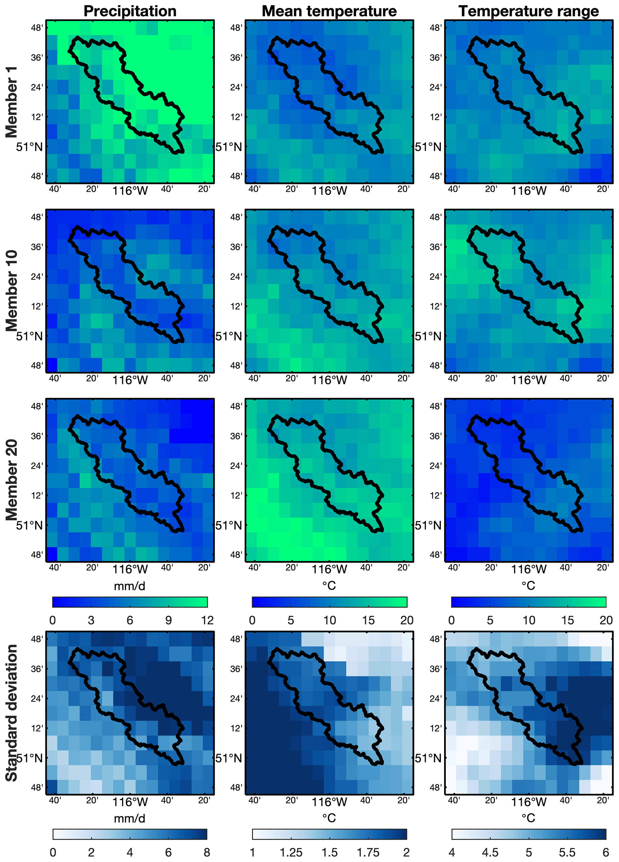
Figure E1The distributions of daily precipitation (the first column), mean daily temperature (the second column), and daily temperature range (the third column) on 29 June 2015. The first to third rows represent ensemble members 1, 10, and 20, respectively. The fourth row represents the standard deviation of 25 members for this day. The black line outlines the Bow River basin above Banff, Canada.
GT and MC designed the framework of this study. GT collected data, performed the analyses, and wrote the paper. MC, SP, AN, and AW contributed to the design of the methodology and result evaluation. SP, DB, and PW contributed to the evaluation of methodology and results. All authors contributed to data analysis, discussions about the methods and results, and paper improvement.
The authors declare that they have no conflict of interest.
Publisher's note: Copernicus Publications remains neutral with regard to jurisdictional claims in published maps and institutional affiliations.
The study is funded by the Global Water Futures (GWF) program in Canada. The authors appreciate the extensive efforts from the developers of the ground and reanalysis datasets to make their products available. The authors also thank the Federated Research Data Repository (FRDR; https://www.frdr-dfdr.ca/repo/; last access: 29 September 2020) for publishing our open-access dataset for users.
This research has been supported by the Global Water Futures (Global Water Futures).
This paper was edited by David Carlson and reviewed by Graham Weedon, Jonathan Gourley, Daniel Wright, and one anonymous referee.
Aalto, J., Pirinen, P., and Jylhä, K.: New gridded daily climatology of Finland: Permutation-based uncertainty estimates and temporal trends in climate, J. Geophys. Res.-Atmos., 121, 3807–3823, https://doi.org/10.1002/2015JD024651, 2016.
Adler, R. F., Gu, G. J., Sapiano, M., Wang, J. J., and Huffman, G. J.: Global Precipitation: Means, Variations and Trends During the Satellite Era (1979–2014), Surv. Geophys., 38, 679–699, https://doi.org/10.1007/s10712-017-9416-4, 2017.
Arias-Hidalgo, M., Bhattacharya, B., Mynett, A. E., and van Griensven, A.: Experiences in using the TMPA-3B42R satellite data to complement rain gauge measurements in the Ecuadorian coastal foothills, Hydrol. Earth Syst. Sci., 17, 2905–2915, https://doi.org/10.5194/hess-17-2905-2013, 2013.
Beck, H. E., Vergopolan, N., Pan, M., Levizzani, V., van Dijk, A. I. J. M., Weedon, G. P., Brocca, L., Pappenberger, F., Huffman, G. J., and Wood, E. F.: Global-scale evaluation of 22 precipitation datasets using gauge observations and hydrological modeling, Hydrol. Earth Syst. Sci., 21, 6201–6217, https://doi.org/10.5194/hess-21-6201-2017, 2017.
Beck, H. E., Wood, E. F., Pan, M., Fisher, C. K., Miralles, D. G., van Dijk, A. I. J. M., McVicar, T. R., and Adler, R. F.: MSWEP V2 Global 3-Hourly 0.1∘ Precipitation: Methodology and Quantitative Assessment, B. Am. Meteorol. Soc., 100, 473–500, https://doi.org/10.1175/BAMS-D-17-0138.1, 2019.
Beck, H. E., Wood, E. F., McVicar, T. R., Zambrano-Bigiarini, M., Alvarez-Garreton, C., Baez-Villanueva, O. M., Sheffield, J., and Karger, D. N.: Bias Correction of Global High-Resolution Precipitation Climatologies Using Streamflow Observations from 9372 Catchments, J. Clim., 33, 1299–1315, https://doi.org/10.1175/JCLI-D-19-0332.1, 2020.
Brier, G. W.: Verification of forecasts expressed in terms of probability, Mon. Weather Rev., 78, 1–3, https://doi.org/10.1175/1520-0493(1950)078<0001:VOFEIT>2.0.CO;2, 1950.
Bromwich, D. H., Wilson, A. B., Bai, L., Liu, Z., Barlage, M., Shih, C.-F., Maldonado, S., Hines, K. M., Wang, S.-H., and Woollen, J.: The Arctic system reanalysis, version 2, B. Am. Meteorol. Soc., 99, 805–828, 2018.
Caillouet, L., Vidal, J.-P., Sauquet, E., Graff, B., and Soubeyroux, J.-M.: SCOPE Climate: a 142-year daily high-resolution ensemble meteorological reconstruction dataset over France, Earth Syst. Sci. Data, 11, 241–260, https://doi.org/10.5194/essd-11-241-2019, 2019.
Cannon, A. J., Sobie, S. R., and Murdock, T. Q.: Bias Correction of GCM Precipitation by Quantile Mapping: How Well Do Methods Preserve Changes in Quantiles and Extremes?, J. Clim., 28, 6938–6959, https://doi.org/10.1175/JCLI-D-14-00754.1, 2015.
Chen, Y., Yuan, W., Xia, J., Fisher, J. B., Dong, W., Zhang, X., Liang, S., Ye, A., Cai, W., and Feng, J.: Using Bayesian model averaging to estimate terrestrial evapotranspiration in China, J. Hydrol., 528, 537–549, https://doi.org/10.1016/j.jhydrol.2015.06.059, 2015.
Clark, M. P. and Hay, L. E.: Use of medium-range numerical weather prediction model output to produce forecasts of streamflow, J. Hydrometeorol., 5, 15–32, 2004.
Clark, M. P. and Slater, A. G.: Probabilistic Quantitative Precipitation Estimation in Complex Terrain, J. Hydrometeorol., 7, 3–22, https://doi.org/10.1175/JHM474.1, 2006.
Clark, M. P., Slater, A. G., Barrett, A. P., Hay, L. E., McCabe, G. J., Rajagopalan, B., and Leavesley, G. H.: Assimilation of snow covered area information into hydrologic and land-surface models, Adv. Water Resour., 29, 1209–1221, https://doi.org/10.1016/j.advwatres.2005.10.001, 2006.
Cornes, R. C., van der Schrier, G., van den Besselaar, E. J. M., and Jones, P. D.: An ensemble version of the E-OBS temperature and precipitation data sets, J. Geophys. Res.-Atmos., 123, 9391–9409, https://doi.org/10.1029/2017JD028200, 2018.
Daly, C., Halbleib, M., Smith, J. I., Gibson, W. P., Doggett, M. K., Taylor, G. H., Curtis, J., and Pasteris, P. P.: Physiographically sensitive mapping of climatological temperature and precipitation across the conterminous United States, Int. J. Climatol., 28, 2031–2064, https://doi.org/10.1002/joc.1688, 2008.
Di Luzio, M., Johnson, G. L., Daly, C., Eischeid, J. K., and Arnold, J. G.: Constructing Retrospective Gridded Daily Precipitation and Temperature Datasets for the Conterminous United States, J. Appl. Meteorol. Climatol., 47, 475–497, https://doi.org/10.1175/2007JAMC1356.1, 2008.
Dinku, T., Anagnostou, E. N., and Borga, M.: Improving radar-based estimation of rainfall over complex terrain, J. Appl. Meteorol., 41, 1163–1178, 2002.
Donat, M. G., Sillmann, J., Wild, S., Alexander, L. V., Lippmann, T., and Zwiers, F. W.: Consistency of Temperature and Precipitation Extremes across Various Global Gridded In Situ and Reanalysis Datasets, J. Clim., 27, 5019–5035, https://doi.org/10.1175/JCLI-D-13-00405.1, 2014.
Duan, Q. and Phillips, T. J.: Bayesian estimation of local signal and noise in multimodel simulations of climate change, J. Geophys. Res.-Atmos., 115, D18123, https://doi.org/10.1029/2009JD013654, 2010.
Duan, S.-B. and Li, Z.-L.: Spatial Downscaling of MODIS Land Surface Temperatures Using Geographically Weighted Regression: Case Study in Northern China, IEEE Trans. Geosci. Remote Sens., 54, 6458–6469, https://doi.org/10.1109/TGRS.2016.2585198, 2016.
Eischeid, J. K., Pasteris, P. A., Diaz, H. F., Plantico, M. S., and Lott, N. J.: Creating a Serially Complete, National Daily Time Series of Temperature and Precipitation for the Western United States, J. Appl. Meteorol., 39, 1580–1591, https://doi.org/10.1175/1520-0450(2000)039<1580:CASCND>2.0.CO;2, 2000.
Fick, S. E. and Hijmans, R. J.: WorldClim 2: new 1 km spatial resolution climate surfaces for global land areas, Int. J. Climatol., 37, 4302–4315, 2017.
Folland, C. K.: Numerical models of the raingauge exposure problem, field experiments and an improved collector design, Q. J. R. Meteor. Soc., 114, 1485–1516, https://doi.org/10.1002/qj.49711448407, 1988.
Fortin, V., Roy, G., Donaldson, N., and Mahidjiba, A.: Assimilation of radar quantitative precipitation estimations in the Canadian Precipitation Analysis (CaPA), J. Hydrol., 531, 296–307, https://doi.org/10.1016/j.jhydrol.2015.08.003, 2015.
Fortin, V., Roy, G., Stadnyk, T., Koenig, K., Gasset, N., and Mahidjiba, A.: Ten Years of Science Based on the Canadian Precipitation Analysis: A CaPA System Overview and Literature Review, Atmos.-Ocean, 56, 178–196, https://doi.org/10.1080/07055900.2018.1474728, 2018.
Frei, C. and Isotta, F. A.: Ensemble Spatial Precipitation Analysis From Rain Gauge Data: Methodology and Application in the European Alps, J. Geophys. Res.-Atmos., 124, 5757–5778, https://doi.org/10.1029/2018JD030004, 2019.
Fuchs, T., Rapp, J., Rubel, F., and Rudolf, B.: Correction of synoptic precipitation observations due to systematic measuring errors with special regard to precipitation phases, Phys. Chem. Earth Pt. B, 26, 689–693, 2001.
Funk, C., Peterson, P., Landsfeld, M., Pedreros, D., Verdin, J., Shukla, S., Husak, G., Rowland, J., Harrison, L., Hoell, A., and Michaelsen, J.: The climate hazards infrared precipitation with stations–a new environmental record for monitoring extremes, Sci. Data, 2, 150066, https://doi.org/10.1038/sdata.2015.66, 2015.
Gelaro, R., McCarty, W., Suárez, M. J., Todling, R., Molod, A., Takacs, L., Randles, C. A., Darmenov, A., Bosilovich, M. G., Reichle, R., Wargan, K., Coy, L., Cullather, R., Draper, C., Akella, S., Buchard, V., Conaty, A., da Silva, A. M., Gu, W., Kim, G.-K., Koster, R., Lucchesi, R., Merkova, D., Nielsen, J. E., Partyka, G., Pawson, S., Putman, W., Rienecker, M., Schubert, S. D., Sienkiewicz, M., and Zhao, B.: The Modern-Era Retrospective Analysis for Research and Applications, Version 2 (MERRA-2), J. Clim., 30, 5419–5454, https://doi.org/10.1175/jcli-d-16-0758.1, 2017.
Goodison, B. E., Louie, P. Y., and Yang, D.: WMO solid precipitation measurement intercomparison, Report no. 67, World Meteorological Organization, 1998.
Habib, E., Haile, A. T., Sazib, N., Zhang, Y., and Rientjes, T.: Effect of Bias Correction of Satellite-Rainfall Estimates on Runoff Simulations at the Source of the Upper Blue Nile, Remote Sens., 6, 6688–6708, https://doi.org/10.3390/rs6076688, 2014.
Hamilton, A. S. and Moore, R. D.: Quantifying Uncertainty in Streamflow Records, Can. Water Resour. J., 37, 3–21, https://doi.org/10.4296/cwrj3701865, 2012.
Harris, I., Osborn, T. J., Jones, P., and Lister, D.: Version 4 of the CRU TS monthly high-resolution gridded multivariate climate dataset, Sci. Data, 7, 109, https://doi.org/10.1038/s41597-020-0453-3, 2020.
Haylock, M. R., Hofstra, N., Klein Tank, A. M. G., Klok, E. J., Jones, P. D., and New, M.: A European daily high-resolution gridded data set of surface temperature and precipitation for 1950–2006, J. Geophys. Res.-Atmos., 113, D20119, https://doi.org/10.1029/2008JD010201, 2008.
Hellinger, E.: Neue begründung der theorie quadratischer formen von unendlichvielen veränderlichen, J.Reine Angew. Math. Crelles J., 1909, 210–271, 1909.
Hempel, S., Frieler, K., Warszawski, L., Schewe, J., and Piontek, F.: A trend-preserving bias correction – the ISI-MIP approach, Earth Syst. Dynam., 4, 219–236, https://doi.org/10.5194/esd-4-219-2013, 2013.
Henn, B., Newman, A. J., Livneh, B., Daly, C., and Lundquist, J. D.: An assessment of differences in gridded precipitation datasets in complex terrain, J. Hydrol., 556, 1205–1219, https://doi.org/10.1016/j.jhydrol.2017.03.008, 2018.
Herrnegger, M., Senoner, T., and Nachtnebel, H.-P.: Adjustment of spatio-temporal precipitation patterns in a high Alpine environment, J. Hydrol., 556, 913–921, https://doi.org/10.1016/j.jhydrol.2016.04.068, 2018.
Hersbach, H.: Decomposition of the continuous ranked probability score for ensemble prediction systems, Weather Forecast., 15, 559–570, 2000.
Hersbach, H., Bell, B., Berrisford, P., Hirahara, S., Horányi, A., Muñoz-Sabater, J., Nicolas, J., Peubey, C., Radu, R., Schepers, D., Simmons, A., Soci, C., Abdalla, S., Abellan, X., Balsamo, G., Bechtold, P., Biavati, G., Bidlot, J., Bonavita, M., Chiara, G. D., Dahlgren, P., Dee, D., Diamantakis, M., Dragani, R., Flemming, J., Forbes, R., Fuentes, M., Geer, A., Haimberger, L., Healy, S., Hogan, R. J., Hólm, E., Janisková, M., Keeley, S., Laloyaux, P., Lopez, P., Lupu, C., Radnoti, G., de Rosnay, P., Rozum, I., Vamborg, F., Villaume, S., and Thépaut, J.-N.: The ERA5 global reanalysis, Q. J. R. Meteorol. Soc., 146, 1999–2049, https://doi.org/10.1002/qj.3803, 2020.
Hoeting, J. A., Madigan, D., Raftery, A. E., and Volinsky, C. T.: Bayesian Model Averaging: A Tutorial, Stat. Sci., 14, 382–401, 1999.
Hong, Y., Hsu, K., Moradkhani, H., and Sorooshian, S.: Uncertainty quantification of satellite precipitation estimation and Monte Carlo assessment of the error propagation into hydrologic response, Water Resour. Res., 42, W08421, https://doi.org/10.1029/2005wr004398, 2006.
Hu, Q., Li, Z., Wang, L., Huang, Y., Wang, Y., and Li, L.: Rainfall Spatial Estimations: A Review from Spatial Interpolation to Multi-Source Data Merging, Water, 11, 579, https://doi.org/10.3390/w11030579, 2019.
Huffman, G. J., Bolvin, D. T., Nelkin, E. J., Wolff, D. B., Adler, R. F., Gu, G., Hong, Y., Bowman, K. P., and Stocker, E. F.: The TRMM Multisatellite Precipitation Analysis (TMPA): Quasi-Global, Multiyear, Combined-Sensor Precipitation Estimates at Fine Scales, J. Hydrometeorol., 8, 38–55, https://doi.org/10.1175/jhm560.1, 2007.
Karger, D. N., Conrad, O., Bohner, J., Kawohl, T., Kreft, H., Soria-Auza, R. W., Zimmermann, N. E., Linder, H. P., and Kessler, M.: Climatologies at high resolution for the earth's land surface areas, Sci. Data, 4, 170122, https://doi.org/10.1038/sdata.2017.122, 2017.
Kemp, W. P., Burnell, D. G., Everson, D. O., and Thomson, A. J.: Estimating Missing Daily Maximum and Minimum Temperatures, J. Clim. Appl. Meteorol., 22, 1587–1593, https://doi.org/10.1175/1520-0450(1983)022<1587:EMDMAM>2.0.CO;2, 1983.
Khedhaouiria, D., Bélair, S., Fortin, V., Roy, G., and Lespinas, F.: High Resolution (2.5 km) Ensemble Precipitation Analysis across Canada, J. Hydrometeorol., 21, 2023–2039, https://doi.org/10.1175/JHM-D-19-0282.1, 2020.
Kiang, J. E., Gazoorian, C., McMillan, H., Coxon, G., Coz, J. L., Westerberg, I. K., Belleville, A., Sevrez, D., Sikorska, A. E., Petersen-Øverleir, A., Reitan, T., Freer, J., Renard, B., Mansanarez, V., and Mason, R.: A Comparison of Methods for Streamflow Uncertainty Estimation, Water Resour. Res., 54, 7149–7176, https://doi.org/10.1029/2018WR022708, 2018.
Kirstetter, P.-E., Gourley, J. J., Hong, Y., Zhang, J., Moazamigoodarzi, S., Langston, C., and Arthur, A.: Probabilistic precipitation rate estimates with ground-based radar networks, Water Resour. Res., 51, 1422–1442, https://doi.org/10.1002/2014WR015672, 2015.
Kobayashi, S., Ota, Y., Harada, Y., Ebita, A., Moriya, M., Onoda, H., Onogi, K., Kamahori, H., Kobayashi, C., Endo, H., Miyaoka, K., and Takahashi, K.: The JRA-55 Reanalysis: General Specifications and Basic Characteristics, J. Meteorol. Soc. Jpn. Ser. II, 93, 5–48, https://doi.org/10.2151/jmsj.2015-001, 2015.
Kochendorfer, J., Nitu, R., Wolff, M., Mekis, E., Rasmussen, R., Baker, B., Earle, M. E., Reverdin, A., Wong, K., Smith, C. D., Yang, D., Roulet, Y.-A., Meyers, T., Buisan, S., Isaksen, K., Brækkan, R., Landolt, S., and Jachcik, A.: Testing and development of transfer functions for weighing precipitation gauges in WMO-SPICE, Hydrol. Earth Syst. Sci., 22, 1437–1452, https://doi.org/10.5194/hess-22-1437-2018, 2018.
Lader, R., Bhatt, U. S., Walsh, J. E., Rupp, T. S., and Bieniek, P. A.: Two-Meter Temperature and Precipitation from Atmospheric Reanalysis Evaluated for Alaska, J. Appl. Meteorol. Climatol., 55, 901–922, https://doi.org/10.1175/JAMC-D-15-0162.1, 2016.
Livneh, B., Rosenberg, E. A., Lin, C., Nijssen, B., Mishra, V., Andreadis, K. M., Maurer, E. P., and Lettenmaier, D. P.: A Long-Term Hydrologically Based Dataset of Land Surface Fluxes and States for the Conterminous United States: Update and Extensions, J. Clim., 26, 9384–9392, https://doi.org/10.1175/JCLI-D-12-00508.1, 2013.
Longman, R. J., Newman, A. J., Giambelluca, T. W., and Lucas, M.: Characterizing the Uncertainty and Assessing the Value of Gap-Filled Daily Rainfall Data in Hawaii, J. Appl. Meteorol. Climatol., 59, 1261–1276, https://doi.org/10.1175/JAMC-D-20-0007.1, 2020.
Lu, X., Tang, G., Wang, X., Liu, Y., Wei, M., and Zhang, Y.: The Development of a Two-Step Merging and Downscaling Method for Satellite Precipitation Products, Remote Sens., 12, 398, https://doi.org/10.3390/rs12030398, 2020.
Ma, Y., Yang, Y., Han, Z., Tang, G., Maguire, L., Chu, Z., and Hong, Y.: Comprehensive evaluation of Ensemble Multi-Satellite Precipitation Dataset using the Dynamic Bayesian Model Averaging scheme over the Tibetan plateau, J. Hydrol., 556, 634–644, https://doi.org/10.1016/j.jhydrol.2017.11.050, 2018a.
Ma, Y., Hong, Y., Chen, Y., Yang, Y., Tang, G., Yao, Y., Long, D., Li, C., Han, Z., and Liu, R.: Performance of Optimally Merged Multisatellite Precipitation Products Using the Dynamic Bayesian Model Averaging Scheme Over the Tibetan Plateau, J. Geophys. Res.-Atmos., 123, 814–834, https://doi.org/10.1002/2017jd026648, 2018b.
Ma, Z., Xu, J., Zhu, S., Yang, J., Tang, G., Yang, Y., Shi, Z., and Hong, Y.: AIMERG: a new Asian precipitation dataset (0.1∘/half-hourly, 2000–2015) by calibrating the GPM-era IMERG at a daily scale using APHRODITE, Earth Syst. Sci. Data, 12, 1525–1544, https://doi.org/10.5194/essd-12-1525-2020, 2020.
Mahfouf, J.-F., Brasnett, B., and Gagnon, S.: A Canadian precipitation analysis (CaPA) project: Description and preliminary results, Atmos.-Ocean, 45, 1–17, https://doi.org/10.3137/ao.v450101, 2007.
Maurer, E. P., Wood, A. W., Adam, J. C., Lettenmaier, D. P., and Nijssen, B.: A Long-Term Hydrologically Based Dataset of Land Surface Fluxes and States for the Conterminous United States, J. Clim., 15, 3237-3251, 2002.
Mears, C. A., Wentz, F. J., Thorne, P., and Bernie, D.: Assessing uncertainty in estimates of atmospheric temperature changes from MSU and AMSU using a Monte-Carlo estimation technique, J. Geophys. Res.-Atmos., 116, D08112, https://doi.org/10.1029/2010JD014954, 2011.
Mendoza, P. A., Wood, A. W., Clark, E., Rothwell, E., Clark, M. P., Nijssen, B., Brekke, L. D., and Arnold, J. R.: An intercomparison of approaches for improving operational seasonal streamflow forecasts, Hydrol. Earth Syst. Sci., 21, 3915–3935, https://doi.org/10.5194/hess-21-3915-2017, 2017.
Mooney, P. A., Mulligan, F. J., and Fealy, R.: Comparison of ERA-40, ERA-Interim and NCEP/NCAR reanalysis data with observed surface air temperatures over Ireland, Int. J. Climatol., 31, 545–557, https://doi.org/10.1002/joc.2098, 2011.
Morice, C. P., Kennedy, J. J., Rayner, N. A., and Jones, P. D.: Quantifying uncertainties in global and regional temperature change using an ensemble of observational estimates: The HadCRUT4 data set, J. Geophys. Res.-Atmos., 117, D08101, https://doi.org/10.1029/2011JD017187, 2012.
Muñoz-Sabater, J., Dutra, E., Agustí-Panareda, A., Albergel, C., Arduini, G., Balsamo, G., Boussetta, S., Choulga, M., Harrigan, S., Hersbach, H., Martens, B., Miralles, D. G., Piles, M., Rodríguez-Fernández, N. J., Zsoter, E., Buontempo, C., and Thépaut, J.-N.: ERA5-Land: A state-of-the-art global reanalysis dataset for land applications, Earth Syst. Sci. Data Discuss. [preprint], https://doi.org/10.5194/essd-2021-82, in review, 2021.
Nešpor, V. and Sevruk, B.: Estimation of Wind-Induced Error of Rainfall Gauge Measurements Using a Numerical Simulation, J. Atmos. Ocean. Tech., 16, 450–464, https://doi.org/10.1175/1520-0426(1999)016<0450:EOWIEO>2.0.CO;2, 1999.
Newman, A. J. and Clark, M. P.: TIER version 1.0: an open-source Topographically InformEd Regression (TIER) model to estimate spatial meteorological fields, Geosci. Model Dev., 13, 1827–1843, https://doi.org/10.5194/gmd-13-1827-2020, 2020.
Newman, A. J., Clark, M. P., Craig, J., Nijssen, B., Wood, A., Gutmann, E., Mizukami, N., Brekke, L., and Arnold, J. R.: Gridded Ensemble Precipitation and Temperature Estimates for the Contiguous United States, J. Hydrometeorol., 16, 2481–2500, https://doi.org/10.1175/JHM-D-15-0026.1, 2015.
Newman, A. J., Clark, M. P., Longman, R. J., and Giambelluca, T. W.: Methodological Intercomparisons of Station-Based Gridded Meteorological Products: Utility, Limitations, and Paths Forward, J. Hydrometeorol., 20, 531–547, https://doi.org/10.1175/JHM-D-18-0114.1, 2019a.
Newman, A. J., Clark, M. P., Longman, R. J., Gilleland, E., Giambelluca, T. W., and Arnold, J. R.: Use of Daily Station Observations to Produce High-Resolution Gridded Probabilistic Precipitation and Temperature Time Series for the Hawaiian Islands, J. Hydrometeorol., 20, 509–529, https://doi.org/10.1175/JHM-D-18-0113.1, 2019b.
Newman, A. J., Clark, M. P., Wood, A. W., and Arnold, J. R.: Probabilistic Spatial Meteorological Estimates for Alaska and the Yukon, J. Geophys. Res.-Atmos., 125, e2020JD032696, https://doi.org/10.1029/2020JD032696, 2020.
Papalexiou, S. M.: Unified theory for stochastic modelling of hydroclimatic processes: Preserving marginal distributions, correlation structures, and intermittency, Adv. Water Resour., 115, 234–252, 2018.
Papalexiou, S. M. and Koutsoyiannis, D.: Battle of extreme value distributions: A global survey on extreme daily rainfall, Water Resour. Res., 49, 187–201, https://doi.org/10.1029/2012WR012557, 2013.
Papalexiou, S. M. and Serinaldi, F.: Random Fields Simplified: Preserving Marginal Distributions, Correlations, and Intermittency, With Applications From Rainfall to Humidity, Water Resour. Res., 56, e2019WR026331, https://doi.org/10.1029/2019WR026331, 2020.
Parker, W. S.: Reanalyses and Observations: What's the Difference?, B. Am. Meteorol. Soc., 97, 1565–1572, https://doi.org/10.1175/BAMS-D-14-00226.1, 2016.
Raftery, A. E., Gneiting, T., Balabdaoui, F., and Polakowski, M.: Using Bayesian Model Averaging to Calibrate Forecast Ensembles, Mon. Weather Rev., 133, 1155–1174, https://doi.org/10.1175/MWR2906.1, 2005.
Rodell, M., Beaudoing, H. K., L'Ecuyer, T. S., Olson, W. S., Famiglietti, J. S., Houser, P. R., Adler, R., Bosilovich, M. G., Clayson, C. A., Chambers, D., Clark, E., Fetzer, E. J., Gao, X., Gu, G., Hilburn, K., Huffman, G. J., Lettenmaier, D. P., Liu, W. T., Robertson, F. R., Schlosser, C. A., Sheffield, J., and Wood, E. F.: The Observed State of the Water Cycle in the Early Twenty-First Century, J. Clim., 28, 8289–8318, https://doi.org/10.1175/JCLI-D-14-00555.1, 2015.
Sampson, A. A., Wright, D. B., Stewart, R. D., and LoBue, A. C.: The role of rainfall temporal and spatial averaging in seasonal simulations of the terrestrial water balance, Hydrol. Process., 34, 2531–2542, https://doi.org/10.1002/hyp.13745, 2020.
Scaff, L., Yang, D., Li, Y., and Mekis, E.: Inconsistency in precipitation measurements across the Alaska–Yukon border, The Cryosphere, 9, 2417–2428, https://doi.org/10.5194/tc-9-2417-2015, 2015.
Schepen, A. and Wang, Q. J.: Model averaging methods to merge operational statistical and dynamic seasonal streamflow forecasts in Australia, Water Resour. Res., 51, 1797–1812, https://doi.org/10.1002/2014WR016163, 2015.
Sevruk, B.: International comparison of national precipitation gauges with a reference pit gauge, WMO Instrum. Obs. Methods Rep. No. 17, 111 pp., 1984.
Shen, Y., Zhao, P., Pan, Y., and Yu, J. J.: A high spatiotemporal gauge-satellite merged precipitation analysis over China, J. Geophys. Res.-Atmos., 119, 3063–3075, https://doi.org/10.1002/2013jd020686, 2014a.
Shen, Y., Zhao, P., Pan, Y., and Yu, J.: A high spatiotemporal gauge-satellite merged precipitation analysis over China, J. Geophys. Res.-Atmos., 119, 3063–3075, https://doi.org/10.1002/2013JD020686, 2014b.
Shen, Y., Hong, Z., Pan, Y., Yu, J., and Maguire, L.: China's 1 km Merged Gauge, Radar and Satellite Experimental Precipitation Dataset, Remote Sens., 10, 264, https://doi.org/10.3390/rs10020264, 2018.
Sinclair, S. and Pegram, G.: Combining radar and rain gauge rainfall estimates using conditional merging, Atmos. Sci. Lett., 6, 19–22, https://doi.org/10.1002/asl.85, 2005.
Slater, A. G. and Clark, M. P.: Snow Data Assimilation via an Ensemble Kalman Filter, J. Hydrometeorol., 7, 478–493, https://doi.org/10.1175/JHM505.1, 2006.
Sun, Q., Miao, C., Duan, Q., Ashouri, H., Sorooshian, S., and Hsu, K.-L.: A Review of Global Precipitation Data Sets: Data Sources, Estimation, and Intercomparisons, Rev. Geophys., 56, 79–107, https://doi.org/10.1002/2017rg000574, 2018.
Tang, G., Zeng, Z., Long, D., Guo, X., Yong, B., Zhang, W., and Hong, Y.: Statistical and Hydrological Comparisons between TRMM and GPM Level-3 Products over a Midlatitude Basin: Is Day-1 IMERG a Good Successor for TMPA 3B42V7?, J. Hydrometeorol., 17, 121–137, https://doi.org/10.1175/jhm-d-15-0059.1, 2016.
Tang, G., Behrangi, A., Long, D., Li, C., and Hong, Y.: Accounting for spatiotemporal errors of gauges: A critical step to evaluate gridded precipitation products, J. Hydrol., 559, 294–306, https://doi.org/10.1016/j.jhydrol.2018.02.057, 2018a.
Tang, G., Behrangi, A., Ma, Z., Long, D., and Hong, Y.: Downscaling of ERA-Interim Temperature in the Contiguous United States and Its Implications for Rain–Snow Partitioning, J. Hydrometeorol., 19, 1215–1233, https://doi.org/10.1175/jhm-d-18-0041.1, 2018b.
Tang, G., Clark, M. P., Papalexiou, S. M., Newman, A. J., Wood, A. W., Brunet, D., and Whitfield, P. H.: EMDNA: Ensemble Meteorological Dataset for North America [Dataset], FRDR, https://doi.org/10.20383/101.0275, 2020a.
Tang, G., Clark, M. P., Papalexiou, S. M., Ma, Z., and Hong, Y.: Have satellite precipitation products improved over last two decades? A comprehensive comparison of GPM IMERG with nine satellite and reanalysis datasets, Remote Sens. Environ., 240, 111697, https://doi.org/10.1016/j.rse.2020.111697, 2020b.
Tang, G., Clark, M. P., Newman, A. J., Wood, A. W., Papalexiou, S. M., Vionnet, V., and Whitfield, P. H.: SCDNA: a serially complete precipitation and temperature dataset for North America from 1979 to 2018, Earth Syst. Sci. Data, 12, 2381–2409, https://doi.org/10.5194/essd-12-2381-2020, 2020c.
Tang, G., Clark, M. P., and Papalexiou, S. M.: The use of serially complete station data to improve the temporal continuity of gridded precipitation and temperature estimates, J. Hydrometeorol., 22, 1553–1568, 2021.
Teutschbein, C. and Seibert, J.: Bias correction of regional climate model simulations for hydrological climate-change impact studies: Review and evaluation of different methods, J. Hydrol., 456–457, 12–29, https://doi.org/10.1016/j.jhydrol.2012.05.052, 2012.
Trenberth, K. E., Dai, A., Rasmussen, R. M., and Parsons, D. B.: The Changing Character of Precipitation, B. Am. Meteorol. Soc., 84, 1205–1218, https://doi.org/10.1175/BAMS-84-9-1205, 2003.
Vila, D. A., de Goncalves, L. G. G., Toll, D. L., and Rozante, J. R.: Statistical Evaluation of Combined Daily Gauge Observations and Rainfall Satellite Estimates over Continental South America, J. Hydrometeorol., 10, 533–543, https://doi.org/10.1175/2008JHM1048.1, 2009.
Weedon, G. P., Balsamo, G., Bellouin, N., Gomes, S., Best, M. J., and Viterbo, P.: The WFDEI meteorological forcing data set: WATCH Forcing Data methodology applied to ERA-Interim reanalysis data, Water Resour. Res., 50, 7505–7514, https://doi.org/10.1002/2014wr015638, 2014.
Willkofer, F., Schmid, F.-J., Komischke, H., Korck, J., Braun, M., and Ludwig, R.: The impact of bias correcting regional climate model results on hydrological indicators for Bavarian catchments, J. Hydrol. Reg. Stud., 19, 25–41, https://doi.org/10.1016/j.ejrh.2018.06.010, 2018.
Wood, A. W., Leung, L. R., Sridhar, V., and Lettenmaier, D. P.: Hydrologic Implications of Dynamical and Statistical Approaches to Downscaling Climate Model Outputs, Clim. Change, 62, 189–216, https://doi.org/10.1023/B:CLIM.0000013685.99609.9e, 2004.
Wu, H., Adler, R. F., Tian, Y., Huffman, G. J., Li, H., and Wang, J.: Real-time global flood estimation using satellite-based precipitation and a coupled land surface and routing model, Water Resour. Res., 50, 2693–2717, https://doi.org/10.1002/2013wr014710, 2014.
Xie, P. and Xiong, A.-Y.: A conceptual model for constructing high-resolution gauge-satellite merged precipitation analyses, J. Geophys. Res.-Atmos., 116, D21106, https://doi.org/10.1029/2011JD016118, 2011.
Xu, S., Wu, C., Wang, L., Gonsamo, A., Shen, Y., and Niu, Z.: A new satellite-based monthly precipitation downscaling algorithm with non-stationary relationship between precipitation and land surface characteristics, Remote Sens. Environ., 162, 119–140, https://doi.org/10.1016/j.rse.2015.02.024, 2015.
Yamazaki, D., Ikeshima, D., Tawatari, R., Yamaguchi, T., O'Loughlin, F., Neal, J. C., Sampson, C. C., Kanae, S., and Bates, P. D.: A high-accuracy map of global terrain elevations, Geophys. Res. Lett., 44, 5844–5853, https://doi.org/10.1002/2017GL072874, 2017.
Yang, D., Goodison, B. E., Ishida, S., and Benson, C. S.: Adjustment of daily precipitation data at 10 climate stations in Alaska: Application of World Meteorological Organization intercomparison results, Water Resour. Res., 34, 241–256, https://doi.org/10.1029/97WR02681, 1998.
Yang, D., Kane, D., Zhang, Z., Legates, D., and Goodison, B.: Bias corrections of long-term (1973-2004) daily precipitation data over the northern regions, Geophys. Res. Lett., 32, L19501, https://doi.org/10.1029/2005gl024057, 2005.
Yin, J., Gentine, P., Zhou, S., Sullivan, S. C., Wang, R., Zhang, Y., and Guo, S.: Large increase in global storm runoff extremes driven by climate and anthropogenic changes, Nat. Commun., 9, 4389, https://doi.org/10.1038/s41467-018-06765-2, 2018.
Zhang, Y., Ren, Y., Ren, G., and Wang, G.: Bias Correction of Gauge Data and its Effect on Precipitation Climatology over Mainland China, J. Appl. Meteorol. Climatol., 58, 2177–2196, https://doi.org/10.1175/JAMC-D-19-0049.1, 2019.
- Abstract
- Introduction
- Datasets
- Methodology
- Results
- Discussion
- Data availability
- Summary and conclusions
- Appendix A: Regression coefficients
- Appendix B: Anomalous stations
- Appendix C: Error of BMA-merged reanalysis estimates
- Appendix D: Metrics for probabilistic evaluation
- Appendix E: Teaser dataset
- Author contributions
- Competing interests
- Disclaimer
- Acknowledgements
- Financial support
- Review statement
- References