Observations from the NOAA P-3 aircraft during ATOMIC

The Atlantic Tradewind Ocean-Atmosphere Mesoscale Interaction Campaign (ATOMIC), part of the larger experiment known as Elucidating the Role of Clouds-Circulation Coupling in Climate (EUREC⁴A), was held in the western Atlantic during the period 17 January–11 February 2020. This paper describes observations made during ATOMIC by the US National Oceanic and Atmospheric Administration's (NOAA) Lockheed WP-3D Orion research aircraft based on the island of Barbados. The aircraft obtained 95 h of observations over 11 flights, many of which were coordinated with the NOAA research ship R/V Ronald H. Brown and autonomous platforms deployed from the ship. Each flight contained a mixture of sampling strategies including high-altitude circles with frequent dropsonde deployment to characterize the large-scale environment, slow descents and ascents to measure the distribution of water vapor and its isotopic composition, stacked legs aimed at sampling the microphysical and thermodynamic state of the boundary layer, and offset straight flight legs for observing clouds and the ocean surface with remote sensing instruments and the thermal structure of the ocean with in situ sensors dropped from the plane. The characteristics of the in situ observations, expendable devices, and remote sensing instrumentation are described, as is the processing used in deriving estimates of physical quantities. Data archived at the National Center for Environmental Information include flight-level data such as aircraft navigation and basic thermodynamic information (NOAA Aircraft Operations Center and NOAA Physical Sciences Laboratory, 2020, https://doi.org/10.25921/7jf5-wv54); high-accuracy measurements of water vapor concentration from an isotope analyzer (National Center for Atmospheric Research, 2020, https://doi.org/10.25921/c5yx-7w29); in situ observations of aerosol, cloud, and precipitation size distributions (Leandro and Chuang, 2020, https://doi.org/10.25921/vwvq-5015); profiles of seawater temperature made with Airborne eXpendable BathyThermographs (AXBTs; NOAA Physical Sciences Laboratory, 2020a, https://doi.org/10.25921/pe39-sx75); radar reflectivity, Doppler velocity, and spectrum width from a nadir-looking W-band radar (NOAA Physical Sciences Laboratory, 2020c, https://doi.org/10.25921/n1hc-dc30); estimates of cloud presence, the cloud-top location, and the cloud-top radar reflectivity and temperature, along with estimates of 10 m wind speed obtained from remote sensing instruments operating in the microwave and thermal infrared spectral regions (NOAA Physical Sciences Laboratory, 2020b, https://doi.org/10.25921/x9q5-9745); and ocean surface wave characteristics from a Wide Swath Radar Altimeter (Prosensing, Inc., 2020, https://doi.org/10.25921/qm06-qx04). Data are provided as netCDF files following Climate and Forecast conventions.

1 Observing the atmosphere and ocean in the wintertime trades

As part of the Atlantic Tradewind Ocean-Atmosphere Mesoscale Interaction Campaign (ATOMIC) the US National Oceanic and Atmospheric Administration (NOAA) operated a Lockheed WP-3D Orion research aircraft from the island of Barbados during the period 17 January–11 February 2020. The aircraft, known formally as N43RF and informally as “Miss Piggy”, is one of two such aircraft in NOAA's hurricane hunter fleet. ATOMIC occurred as part of the field campaign EUREC⁴A (Elucidating the Role of Clouds-Circulation Coupling in Climate; see Bony et al., 2017) focusing on relationships between oceanic shallow trade cumulus clouds and their environment, including the role of air–sea interactions.

ATOMIC included a cruise by the NOAA ship Ronald H. Brown (RHB) and deployments of autonomous aircraft and ocean vehicles. Measurements from the ocean platforms are described in Quinn et al. (2021). The main experimental area for EUREC⁴A was just east of Barbados. Both the P-3 and the RHB primarily operated east of the EUREC⁴A area (i.e., east of 57^∘ E), nominally upwind, within the “Tradewind Alley” (see Stevens et al., 2021) extending eastwards from the island of Barbados towards the Northwest Tropical Atlantic Station buoy near 15^∘ N, 51^∘ W. Many of the 11 P-3 flights included excursions to the location of the RHB and sampling of atmospheric and oceanic conditions around the ship and other ocean vehicles. Because of its large size and long endurance (most flights were 8–9 h long) the P-3 was tasked with obtaining a wide array of observations including remote sensing of clouds and the ocean surface, in situ measurements within and below clouds and of isotopic composition throughout the lower troposphere, and the deployment of expendable profiling instruments in the atmosphere and ocean.

This paper describes observations made by the P-3 aircraft during ATOMIC. The next section describes the flights during which the measurements were obtained, including the flight plans designed to meet each objective. Instrumentation is described in Sect. 3. Data processing, including the calculation of derived quantities from one or more instruments, is detailed in Sect. 4, which also includes examples and select comparisons with measurements made by other platforms. Some measurements obtained from the P-3 are or will be included in cross-experiment datasets described elsewhere.

2 Sampling strategy

ATOMIC's goals, as the name implies, include illuminating the role of mesoscale circulations in the ocean and atmosphere as they influence the coupling between the two. As a result the flight strategies included a mix of four different kinds of segments.

1. High-altitude (nominally 24 000 ft/7.5 km) circles, nominally of 90 km radius, during which 12 dropsondes (see Sect. 3.2.1) were deployed to characterize the large-scale vertical motion (Lenschow et al., 2007; Bony and Stevens, 2019). Many of the dropsonde circles were centered on the position of the Ronald H. Brown; others were in the location near Barbados that was routinely sampled by the German HALO aircraft. During daytime flights these were typically the first pattern flown.

2. Slow descents and ascents to sample thermodynamic profiles and the isotopic composition of water vapor (see Sect. 3.1.2). This pattern was usually flown at the end of the first dropsonde circle, descending from the circle level to 500 ft/150 m above the surface and then ascending to the flight level required for the next pattern.

3. In situ cloud sampling patterns, a series of vertically stacked straight and level legs at altitudes determined during flight. These altitudes were chosen to sample near the ocean surface, just below cloud base, one or more levels within the cloud layer, and just above it, allowing for the calculation of fluxes based on measurements of temperature, wind, and humidity (see Sect. 3.1.1 and 3.1.2) and cloud and aerosol size distributions (see Sect. 3.1.3). The location of these patterns was determined by the presence and characteristics of the clouds on the flight day.

4. Sets of horizontally offset long straight legs (“lawnmower patterns”) designed to sample the co-variability of clouds and the ocean, emphasizing observations of ocean temperature profiles (Sect. 3.2.2) and the characteristics of ocean surface waves (Sect. 3.3.2). These patterns were flown at 9000–10 000 ft/2.75–3 km so the aircraft could be depressurized to deploy Airborne eXpendable BathyThermographs (AXBTs); this altitude also provides good sensitivity for remote sensing of the ocean surface and clouds. These flight patterns were placed over regions of sea surface temperatures gradients and/or areas being sampled by autonomous ocean vehicles (surface drifters, wave gliders) deployed from the Ronald H. Brown.

Transits between Barbados and the daily operating area offered further opportunities for deploying dropsondes and AXBTs and for remote sensing. The P-3 flew 11 flights during ATOMIC for a total of 95 h. The first eight flights took place during the day, with nominal takeoff times at 13:00 UTC (09:00 local time); the last three took place overnight, with takeoff times between 02:00–03:30 UTC (local times between 22:00 and 23:30 the previous day). Table 1 provides an overview of sampling strategies and other information for each flight. A plan (map) view of the flight tracks is shown in Fig. 1; altitudes are shown as a function of flight time in Fig. 2.

Table 1 Flight sampling strategies employed on each flight by the P-3 during ATOMIC. Flight date is UTC and most flights were 8–9 h long. Numbers in parentheses show the number of AXBTs for which valid data were obtained. “RHB” indicates that the R/V Ronald H. Brown was at the center of a dropsonde circle. Most AXBT patterns deployed 20 instruments. “Cloud” indicates the number of cloud patterns flown; each typically involved sampling at four or five altitudes. See also Table 3 of Quinn et al. (2021). Detailed reports from each flight are available at the EUREC⁴A data portal (https://observations.ipsl.fr/aeris/eurec4a/, last access: 11 June 2021).

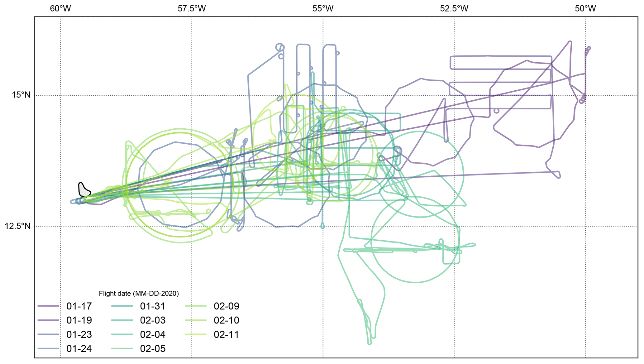
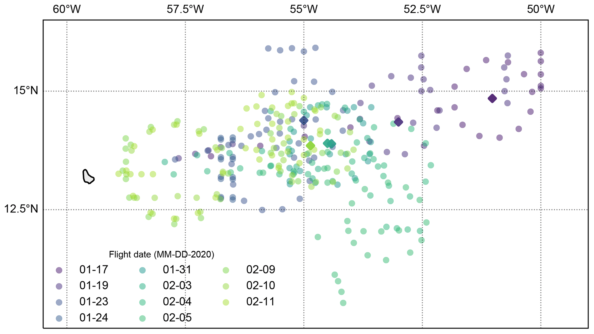
Figure 1 Flight tracks for the 11 flights made by the NOAA P-3 aircraft during ATOMIC on a map with the island of Barbados at left center. Most dropsondes were deployed from regular dodecagons during the first part of the experiment with short turns after each dropsonde providing an off-nadir look at the ocean surface useful for calibrating the W-band radar. A change in pilots midway through the experiment led to dropsondes being deployed from circular flight tracks starting on 31 January. AXBTs were deployed in lawnmower patterns (parallel offset legs) with small loops sometimes employed to lengthen the time between AXBT deployment to allow time for data acquisition given the device's slow fall speeds. Profiling and especially in situ cloud sampling legs sometimes deviated from straight paths to avoid hazardous weather. The color coding is drawn from a palette spanning the length of the experiment, so that days that are close in time have similar colors.

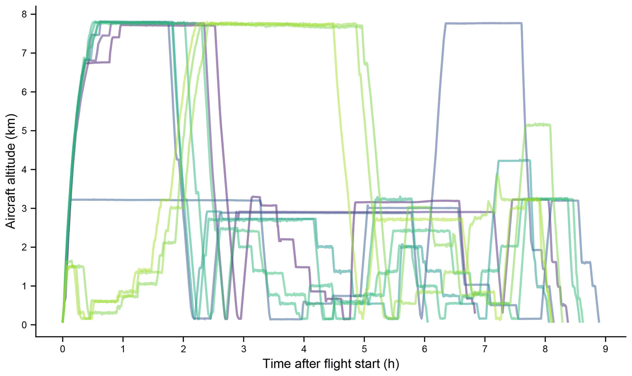
Figure 2 Flight altitude as a function of time after takeoff for the 11 flights by the NOAA P-3 aircraft during ATOMIC, using the same colors as Fig. 1. Sondes were dropped from ∼7.5 km, with each circle taking roughly an hour; transits were frequently performed at this level to conserve fuel. Long intervals near 3 km were used to deploy AXBTs and/or characterize the ocean surface with remote sensing. Stepped legs indicate times devoted to in situ cloud sampling. On most flights the aircraft climbed quickly to roughly 7.5 km, partly to deconflict with other aircraft participating in the experiment. On the three night flights, however, no other aircraft were operating at takeoff times and cloud sampling was performed first, nearer Barbados than on other flights.

3 Instrumentation and initial data processing

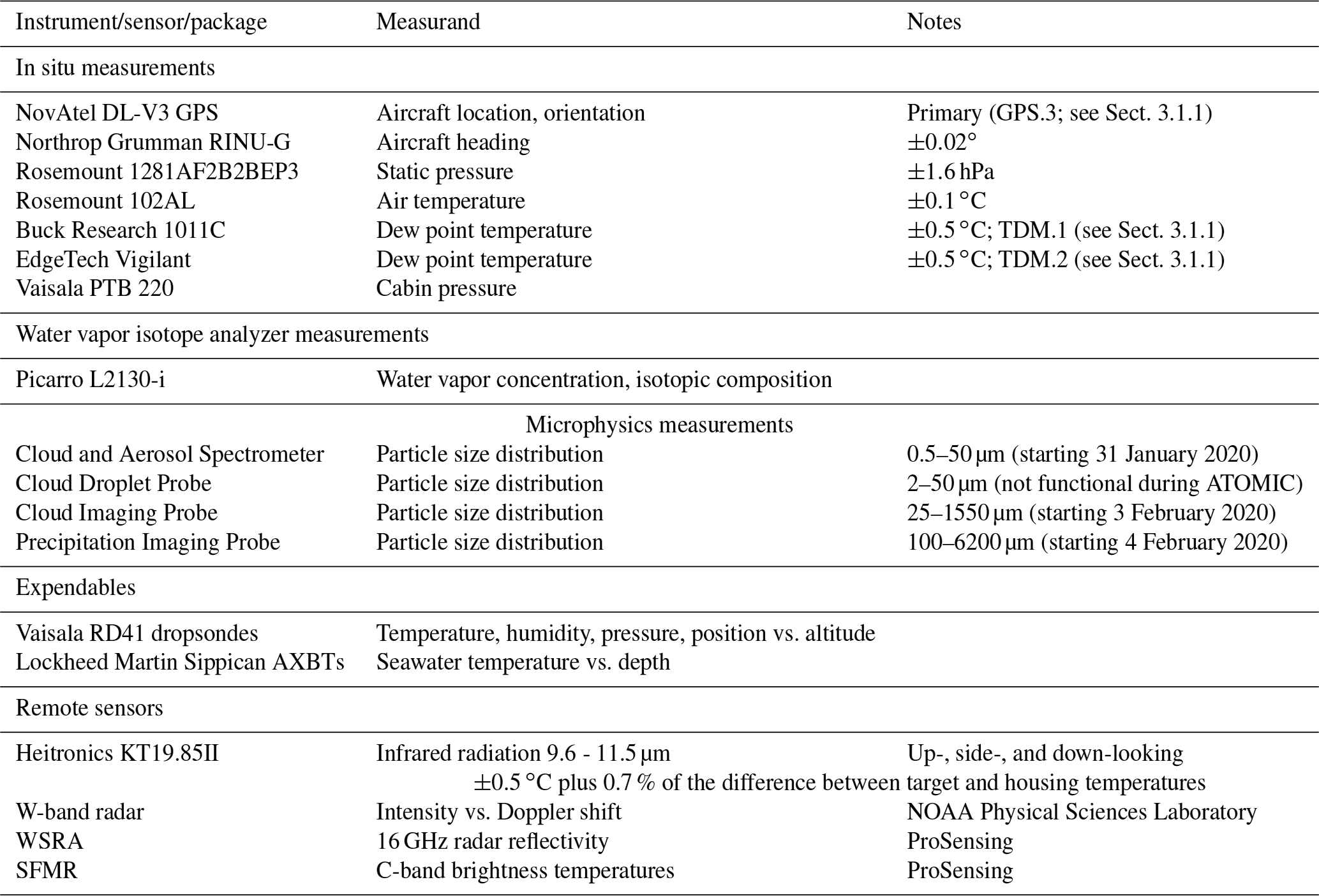
Table 2 describes the instrumentation on and deployed from the P-3 during ATOMIC. The instrumentation was similar to that used during hurricane reconnaissance flights and other scientific missions with the exception of the water vapor isotope analyzer provided by the National Center for Atmospheric Research (see Sect. 3.1.2) and the nadir-looking W-band cloud radar provided by NOAA's Physical Sciences Laboratory (Sect. 3.3.1). Many of the basic in situ measurements are combined to provide derived quantities (e.g., wind speed, relative humidity) described in Sect. 4.

Table 2 Instrumentation aboard or deployed from the P-3 aircraft during the ATOMIC field campaign. Most instruments are the same or similar to those used during hurricane reconnaissance and other scientific missions, though the water vapor isotope analyzer and W-band radar were deployed specifically for this field campaign. See also Table A5 in Stevens et al. (2021).

3.1 In situ measurements

3.1.1 Flight level data

Flight level data are recorded every second from the sensors installed on the P-3 via the Airborne Atmospheric Measurement and Profiling System (AAMPS). Some quantities are measured by multiple sensors; such values are denoted within files prepared by NOAA's Aircraft Operations Center (AOC) with a trailing integer for each independent measurement (e.g., TDM.1, TDM.2, and TDM.3 denote dew point temperature measurements from three independent sensors). Flight level data were post-processed and quality controlled by the flight directors (authors Quinn T. Kalen and Ashley Lundry during ATOMIC) after each flight, typically within a day during the campaign. Each sensor's data are verified to ensure that they represent sound meteorological conditions for that given instrument and then are marked as valid on the QC checklist included in the Mission Documents (available from https://seb.noaa.gov/pub/acdata/2020/MET/ (last access: 11 June 2021) in directories labeled by flight date and the letter “I” to denote N43RF). In cases where there is more than one reliable sensor, one sensor is set as the reference, i.e., TDMref. The reference sensor is chosen to minimize data intermittency and maximize both comparisons to independent measurements (e.g., temperature may be compared to dropsondes) and self-consistency among measurements. The intent is to choose a single sensor which best represents the flight overall, even if this sensor might have periods of bad data (e.g., overshooting by the chilled-mirror dew point sensors) during the flight when other sensors might be more reliable. Additional parameters are derived (variable names end in “.d”) and corrected (variable names end in “.c”) from these data. AOC produces and distributes one netCDF file per flight. Both raw data and the AOC summary file are available for all flights from NOAA's National Center for Environmental Information (see https://www.ncei.noaa.gov/metadata/geoportal/rest/metadata/item/gov.noaa.ncdc:C00581/html, last access: 11 June 2021, where files may be selected by project).

3.1.2 Water vapor stable isotope analyzer

During ATOMIC the P-3 was equipped with a flight-ready Picarro L2130-i water vapor isotopic analyzer which measured the concentration of water vapor and its isotopic composition at 5 Hz frequency. ATOMIC was the first flight campaign for this newly developed instrument although similar instruments have flown as part of previous airborne research missions (e.g., Sodemann et al., 2017; Herman et al., 2020). The isotope ratio measurements, which are part of a broad suite of such observations made during EUREC⁴A, are reported elsewhere; here we describe the instrument's fast and accurate measurements of water vapor concentration (i.e., mixing ratio).

While in flight, the isotopic analyzer drew in ambient air through a backwards-facing 0.25 in./6.35 mm copper tube, centered within a National Center for Atmospheric Research HIAPER Modular Inlet (HIMIL). This ensured the selective sampling of water vapor (versus total water). Because mass but not volumetric flow was controlled through the copper tubing, the time delay (τ in seconds) for air entering the HIMIL to reach the isotopic analyzer varied as a function of pressure and temperature. This delay may be approximated as $\mathit{\tau }=\mathrm{1.0748}p/T_{\mathrm{set}}$, where T_set is the set point (K) of the heaters wrapping the copper tubing inside the aircraft cabin, p is the ambient pressure (hPa) recorded by the aircraft, and the constant (units of s K hPa⁻¹) represents both the best approximation for the inner volume of the copper tube, including the 6 ft/183 cm inside the cabin and 1 ft/30.5 cm extending out through the HIMIL pylon, and the scale factor required to relate T_set and p to the standard conditions under which the volumetric flow rate of the isotopic analyzer is known. The tube inside the cabin was heated to 313.15 K during the first two flights and 321.15 K thereafter, resulting in a typical time delay of 3.4±0.3 s near the surface, which reduces by approximately 1 s for every 300 hPa gained in altitude. Not all parameters in this equation are well constrained or fully representative of the exact sampling conditions within the inlet; the uncertainty in τ may be roughly estimated by considering p±75 hPa.

Mixing of water vapor within the inlet system, and with molecules that have adsorbed to the copper tubing, also partially smooths high-frequency signals (Aemisegger et al., 2012). These effects are, however, fairly small and consistent across flights. The aircraft hygrometer's time response, in contrast, is quite variable and depends on flight conditions, and the hygrometer is subject to both overshooting (e.g., when the measured signal surpasses the expected value following a rapid rise in environmental water vapor concentration) and ringing (i.e., rapid oscillations around the expected value) during rapid and large changes in water vapor concentration. This is illustrated in Fig. 3, which also highlights the hygrometer's much slower time response (as compared to the isotopic analyzer) in the low-humidity conditions found at the highest flight altitudes. Outside of these time periods, the agreement between the hygrometer and isotopic analyzer is quite good (lower panel). Given the more consistently accurate measurements of the isotopic analyzer during ATOMIC, we recommend its use in preference to the aircraft hygrometer for characterizing the thermodynamic state of the atmosphere.

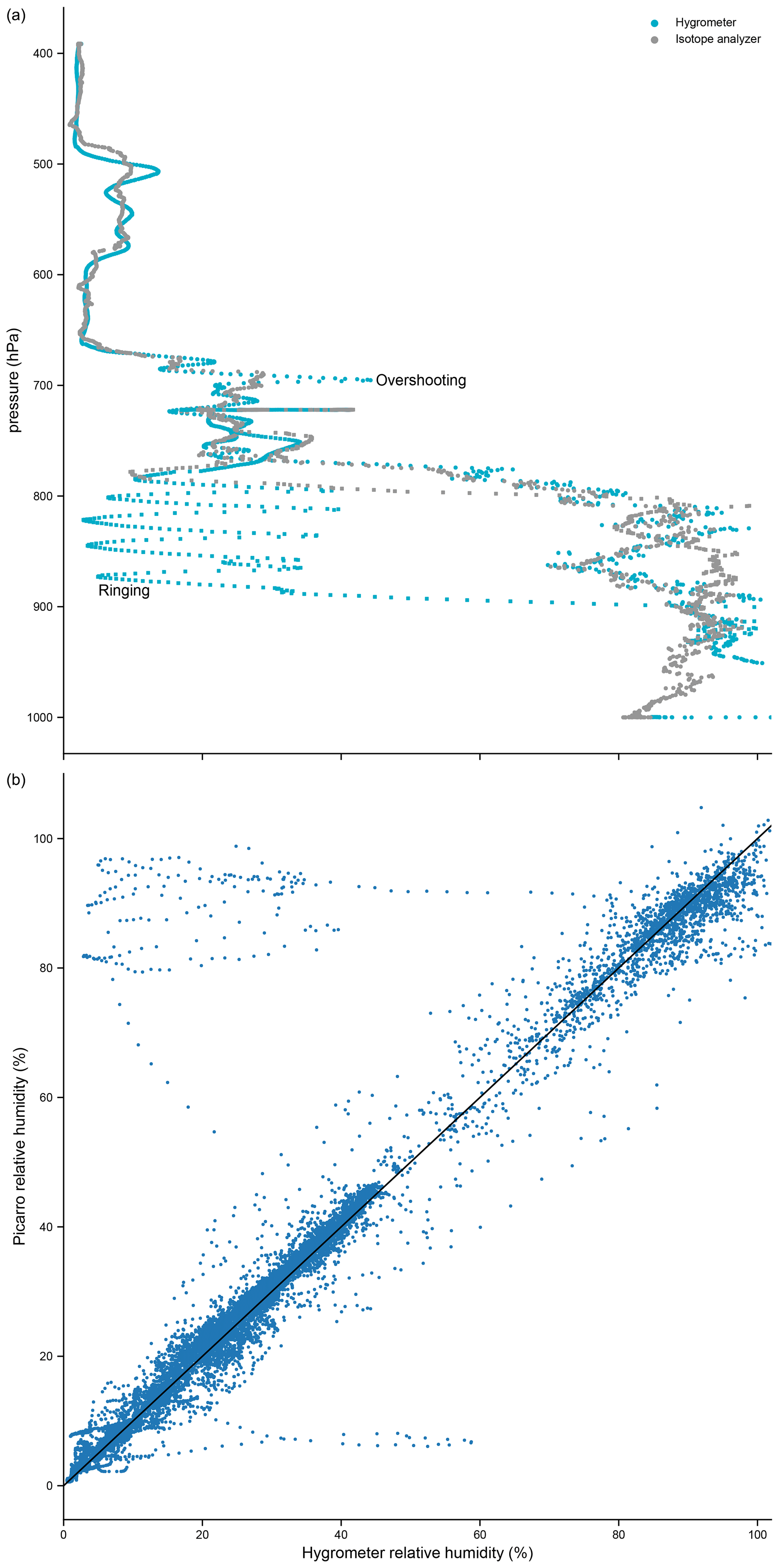
Figure 3 (a) Vertical profiles of relative humidity from the P3 hygrometer (teal) on 19 January 2020 show overshooting, ringing, and a slow time response under the low-humidity conditions found at the highest flight altitudes. These features are absent in the relative humidity profiles estimated from the water vapor isotopic analyzer (grey). Data in this panel are taken in two time windows (15:36:00 to 16:07:40 UTC, shown as circles, and 20:31:12 to 20:41:16 UTC, shown in squares) encompassing two separate slow profiles. (b) Relative humidity as measured by the two sensors over the entire flight. The black line indicates equality. There is good agreement between the two water vapor sensors when relative humidity exceeds ∼20 % and when the hygrometer is not ringing or overshooting.

3.1.3 Microphysics

A number of instruments for measuring aerosol and hydrometeor microphysical properties were aboard the P-3 during ATOMIC. All devices listed in Table 2 are standard instrumentation manufactured by Droplet Measurement Technologies. A Cloud and Aerosol Spectrometer (CAS; nominal diameter range 0.5 to 50 µm) and a Cloud Droplet Probe (CDP; nominal diameter range 2 to 50 µm) were deployed to measure aerosols and cloud suspended cloud particles. Precipitation drops were measured with a Cloud Imaging Probe (CIP; nominal diameter range 25 µm to 1.55 mm) and a Precipitation Imaging Probe (PIP; nominal diameter range 100 µm to 6.2 mm). All instruments were factory-calibrated immediately before the project.

Microphysics measurements were not made during all ATOMIC flights. The computer controlling the microphysical instruments failed on the first flight and took some time to replace so that no microphysical measurements were made during the first four flights. The CDP never functioned properly during the experiment, while the CIP did not function until the sixth flight on 3 February 2020 and the PIP until the seventh flight on 4 February 2020. Measurements are available from all other instruments for all remaining flights up to the end of the project.

3.2 Expendable instrumentation

3.2.1 Dropsondes

The P-3 released 320 Vaisala RD41 dropsondes during ATOMIC at the locations shown in Fig. 4. Most were released from 24 000 ft/7.5 km, though some were released from slightly lower altitudes during transits and others from 9000–10 000 ft/2.75–3 km during cloud and AXBT flight patterns. The RD41 sensors measures pressure, temperature, and humidity as the package falls from the plane, slowed by a parachute (Hock and Franklin, 1999). A GPS package provides location from which wind direction and wind speed are calculated and reported in real time. Measurements are available from the aircraft flight level to the ocean surface. Dropsondes from the P-3 were processed in real time during flight and made available for assimilation over the Global Telecommunications System.

Figure 4 Location of dropsondes deployed during ATOMIC. Most circles (see Table 1) were centered on the position of the R/V Ronald H. Brown; the ship's position at the start of the circle is shown with a diamond.

3.2.2 AXBTs

A total of 165 AXBT instruments (Bane and Sessions, 1984; Dinegar Boyd, 1987; Alappattu and Wang, 2015) were deployed from the P-3 over seven flights at locations shown in Fig. 5. Most were released at or near 9000 ft/2.75 km. The AXBTs, manufactured by Lockheed Martin Sippican, collect ocean temperature as a function of time after launch. AXBTs normally begin transmitting data when the sensor enters the ocean. One file was produced for each AXBT sensor by removing any extraneous observations obtained before splashdown and then converting time to depth assuming a nominal in-water fall speed of 1.594 m s⁻¹. Location is determined from the aircraft navigational information at the time the AXBT was released. A median filter was applied to remove most (but not all) spurious outliers in ocean water temperature.

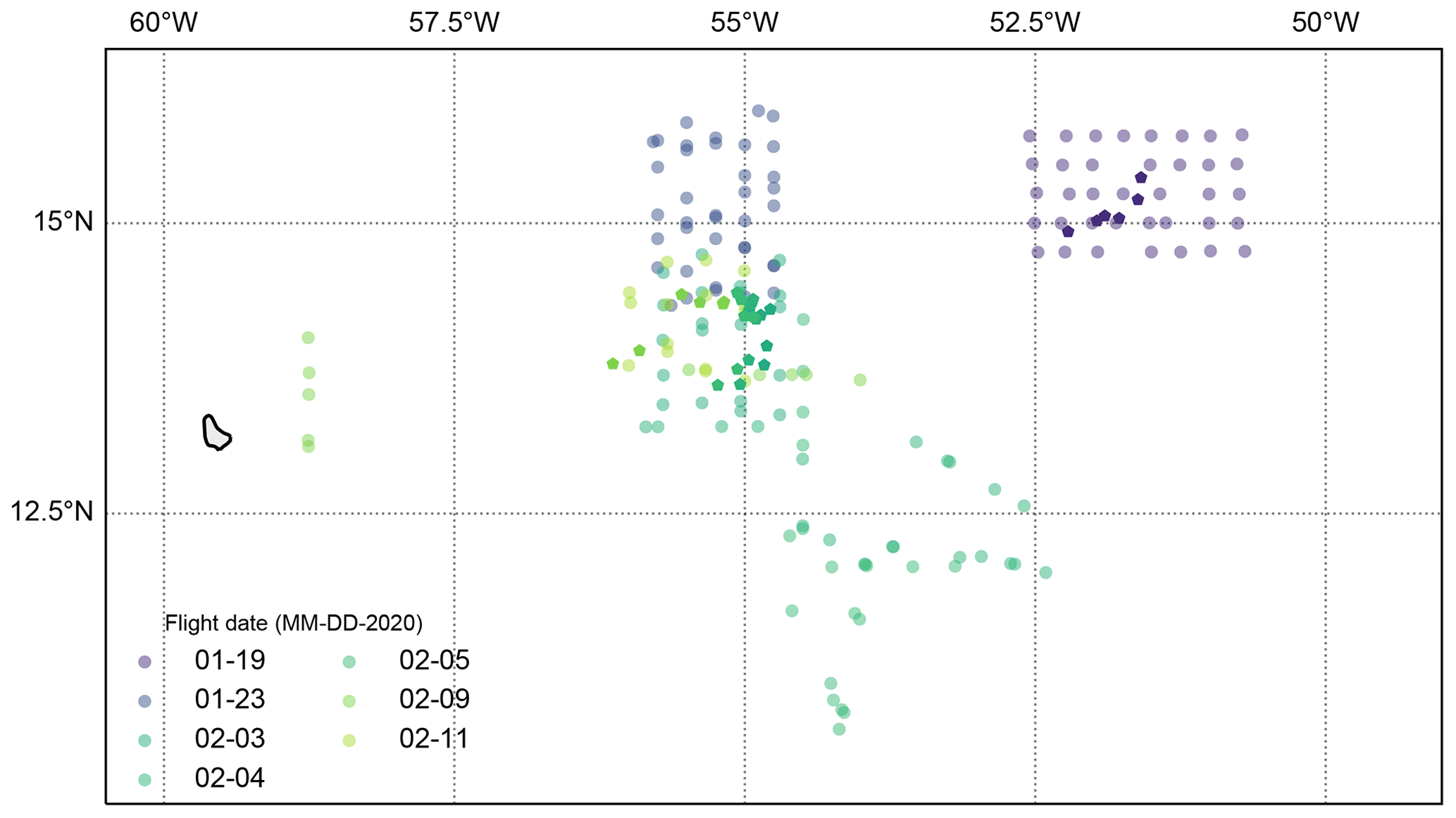
Figure 5 Location of AXBTs deployed during ATOMIC. Many were deployed in lawnmower patterns around the five drifting Surface Wave Instrument Float with Tracking (SWIFT) buoys described in Quinn et al. (2021); the positions of the buoys at the mid-point of the AXBT deployment is denoted with pentagons.

3.3 Remote sensing observations

3.3.1 Physical Sciences Laboratory W-band radar

Remote sensing instrumentation on the P-3 during ATOMIC included the NOAA Physical Sciences Laboratory (PSL) W-band (94 GHz) pulsed Doppler radar. The hardware and processing are described in Moran et al. (2012). It has been deployed from the surface (ships and land stations) looking up and from NOAA P-3 aircraft looking down. In ATOMIC the airborne radar was operated with 220 30 m range gates with a dwell time of 0.5 s. The minimum detectable reflectivity is −36 dBZ at a range of 1 km, although accurate estimates of Doppler properties require about −30 dBZ at 1 km. A similar instrument was deployed on the RHB (Quinn et al., 2021).

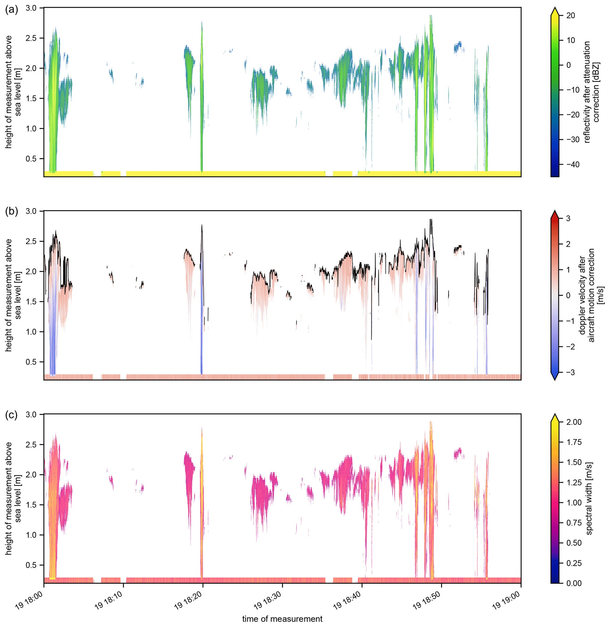
Figure 6 One example hour (18:00–19:00 UTC on 19 January 2020) of observations made by the W-band radar during ATOMIC. Panel (a) shows attenuation-corrected radar reflectivity (dBZ); panel (b) shows the Doppler velocity after correction for aircraft motion (m s⁻¹); panel (c) shows the the width of the Doppler spectrum (m s⁻¹). Observations with radar signal-to-noise ratio of less than −10 dB have been removed for clarity. Clouds observed during this hour were relatively deep, frequently reaching 2.5–3 km, with frequent periods of rain visible in the high-reflectivity, negative Doppler velocity (drops moving away from the aircraft, i.e., falling, in blue), and enhanced spectral width extending from near cloud top to the surface. During ATOMIC, clouds without precipitation typically have reflectivity less than −25 dBZ; in this figure small precipitation drops (green colors in the reflectivity panel) are embedded in the clouds most of the time. The radar has sufficient sensitivity to see these weak returns out to about 2 km below the aircraft (about 1 km altitude). Doppler width is broadened by the aircraft flight speed, which adds a threshold of about 0.5 m s⁻¹.

Radar data were post-processed following Fairall et al. (2018). Standard processing produces vertical profiles of estimates of reflectivity, Doppler velocity, spectrum width, and cloud-free signal-to-noise ratio, converted to a uniform grid referenced to the sea surface rather than as distance from the aircraft. Reflectivity profiles are corrected for attenuation by atmospheric gases and precipitation. Absorption by water vapor and oxygen is calculated based on temperature, pressure, and relative humidity profiles measured by dropsondes using the model suggested by the ITU-R (2013). Attenuation by precipitation is estimated using inversions and relationships from Hitschfeld and Bordan (1954) following Iguchi and Meneghini (1994). Measured Doppler velocity is corrected for the pitch and roll components of aircraft motion. The vertical speed of the aircraft is calculated from flight level data (Sect. 3.1.1) and taken into account in the Doppler velocity correction especially during aircraft ascents and descents. An example from an hour of flight (18:00–19:00 UTC on 19 January) is shown in Fig. 6.

3.3.2 Wide Swath Radar Altimeter

The NOAA Wide Swath Radar Altimeter (WSRA; see Walsh et al., 2014; PopStefanija et al., 2020), developed and manufactured by ProSensing, Inc. of Amherst, MA, USA, is a digital beam-forming radar altimeter operating at 16 GHz in the Ku band. It generates 80 narrow beams spread over ±30^∘ to produce a topographic map of the sea surface waves and their backscattered power. These measurements allow for continuous reporting of directional ocean wave spectra and quantities derived from this including significant wave height, sea surface mean square slope, and the height, wavelength, and direction of propagation of primary and secondary wave fields. Rainfall rate is estimated from path-integrated attenuation (Walsh et al., 2014).

3.3.3 Stepped Frequency Microwave Radiometer

The Stepped Frequency Microwave Radiometer (SFMR) is a nadir-looking microwave radiometer also built by ProSensing. The instrument measures brightness temperatures of the ocean surface and intervening atmosphere at six C-band (4–7 GHz) frequencies. Surface wind speed and average columnar rain rate can be inferred from these brightness temperature values (Uhlhorn et al., 2007). The current implementation (Sapp et al., 2019) has its origins in prototypes developed by the Microwave Remote Sensing Laboratory at the University of Massachusetts and NOAA's Hurricane Research Division and deployed in 1980; the hardware and retrieval methods have been improved several times since.

3.3.4 Infrared radiometer

The P-3 deployed three Heitronics KT19.85 passive infrared radiometers which measure radiation in the 9.6–11.5 µm spectral range. One radiometer points horizontally out the port side of the plane; the others are zenith- nadir-looking. Measured radiation is converted to a brightness temperature. This system has a resolution of 0.1 ^∘C and an accuracy of 0.5 ^∘C plus 0.7 % of the difference between the target and instrument housing temperatures. The field of view is 0.5^∘ and the response time is approximately 0.5 s.

4 Post-processed and derived quantities

Data obtained during the experiment have been post-processed and a variety of derived quantities, as described in this section, have been produced. Data files are organized topically as described in Table 3 and explained more fully in this section. One file per day is provided for each of the entries in the table. All data are archived at the US National Center for Environmental Information.

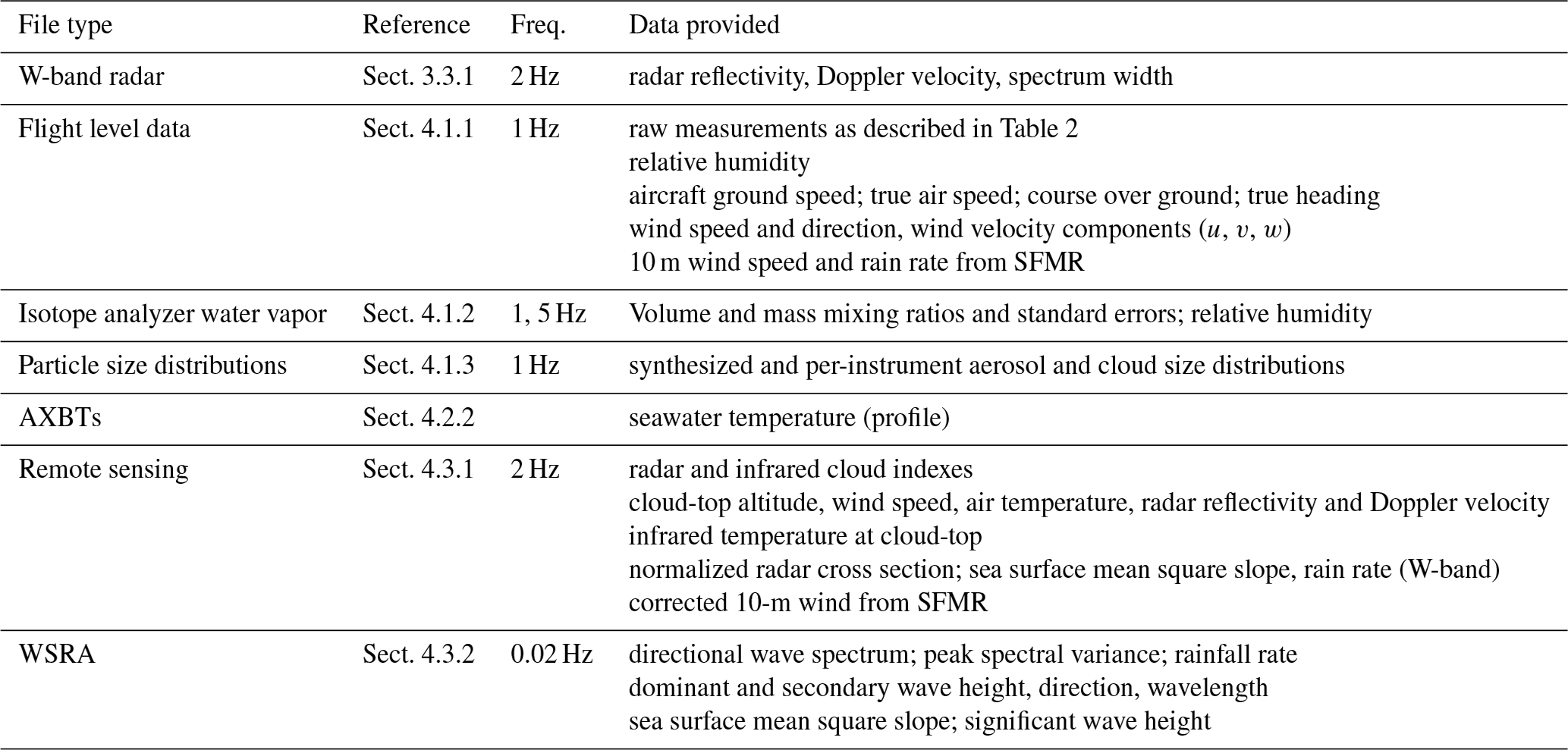
Table 3 Data available from the P-3 during ATOMIC. Data are packaged as one file per type per flight day. Subsections within Sect. 4 describe the production of data beyond routine flight level data (Sect. 3.1.1) and the routinely processed radar observations (Sect. 3.3.1).

4.1 In situ data

4.1.1 Flight level data

To simplify analysis and ease comparisons to other observations we have produced modestly reformatted data files containing a subset of flight level data. These files contain only the reference value of quantities measured by multiple sensors. Some variables are renamed for consistency with other platforms in ATOMIC and/or EUREC⁴A. Metadata are added or otherwise made consistent with conventions developed for the experiments. The dataset includes measurements of vertical velocity measurements made at 1 Hz; these represent the only in situ measurements of turbulence made by the P-3.

4.1.2 Isotope analyzer

Water vapor measurements from the isotopic analyzer are proportional to the ratio of the moles of water vapor to the moles of moist air (dry air plus water vapor) and are reported as a volume mixing ratio in parts per million volume (ppmv). These are provided alongside estimates of the mass mixing ratio – the ratio of the mass of water vapor to the mass of dry air – at both the analyzer's native time resolution of nominal 5 Hz frequency and at a reduced resolution of 1 Hz aligned with the P-3 aircraft data system through boxcar averaging. For convenience, estimates of relative humidity are also provided, obtained by multiplying the 1 Hz volume mixing ratios by the aircraft static (ambient) pressure measurements and dividing by the saturation vapor pressure, estimated from the aircraft ambient temperature following Hardy (1998).The files are aligned in time with the flight level data.

The isotopic analyzer's water vapor measurements have been corrected for a low bias of increasing magnitude at concentrations exceeding 10 000 ppmv, identified using a LI-COR 610 dew point generator. The uncertainty associated with this correction spans 26 to 29 ppmv for the humidity range 200 to 30 000 ppmv but reduces to 12 ppmv upon averaging to 1 Hz. The accuracy of volume mixing ratios below 200 ppmv is unverified.

4.1.3 Microphysics

Particle size distributions for microphysical instruments are processed at 1 Hz resolution for each day where data were available. The CAS and CDP are processed with standard codes available from the manufacturer (although, as noted in Sect. 3.1.3, the CDP did not produce useful data during ATOMIC and is therefore not included in the final archived product). The CIP and PIP provide quick-look data that are qualitatively useful, but accurate quantitative data require specialized processing of the individual particle images. The System for OAP Data Analysis version 2 (SODA-2, https://github.com/abansemer/soda2, last access: 11 June 2021) is used to process the images to produce drop size distributions from both instruments. For the PIP, accurate sizing of particles up to 30 mm is possible in post-processing. However, particles larger than approximately 6 mm are typically ice particles; any such particles in the data should be ignored.

An aerosol size distribution is inferred from measurements that range from 0.5 to 2 µm in size collected by the CAS. (Larger particles are included in the hydrometeor size distribution.) The division is motivated by size distributions observed during ATOMIC, which usually included two modes with the minimum between them typically close to 2 µm. Aerosol concentrations collected in cloud are higher than expected. This may be a result of cloud drop shattering at the CAS inlet, so these measurements should be treated with caution. We do not anticipate that we can correct this potential issue due to corruption of the CAS particle-by-particle files during the campaign.

Measurements collected by the CAS, CIP, and PIP at 1 Hz resolution are synthesized to generate a merged size distribution for hydrometeors ranging from 2 to 30 µm. The CAS, CIP, and PIP are used exclusively for hydrometeors in the size ranges of 2–50 µm, 50–400 µm, and 1.8–30 mm, respectively, although concentration of particles greater than 6 mm should not be considered reliable. For hydrometeors in the size range of 400 µm–1.8 mm, CIP observations are re-binned to the same size bins as the PIP and a sample volume-weighted average is computed. Figure 7 shows an example of the size distribution for each instrument along with the merged hydrometeor distribution. These are altitude-averaged size distributions for one cloud module leg on 5 February 2020 from 19:51:48 to 20:07:18 UTC.

Quick-look videos are available for each cloud module. Each video is approximately 1 min in duration and displays aircraft altitude and the flight track superimposed on visible satellite imagery, along with second-by-second hydrometeor size distributions and scalar measures of this distribution (liquid water content, total number concentration, and Sauter mean or effective diameter) while in cloud, leg averages for these quantities, and the time spent in cloud for each cloud module leg. These videos are available alongside the numerical data.

Figure 7 Size distributions for the CAS, CIP, and PIP (colored rectangles) along with the merged hydrometeor distribution (black line) synthesized from all three instruments. The figure demonstrate the re-binning described in the text. The figure shows data from a single cloud pattern leg on 5 February 2020 from 19:51:48 to 20:07:18 UTC.

4.2 Expendables

4.2.1 Dropsondes

Observations from the dropsondes (Sect. 3.2.1) deployed by the P-3 were processed alongside similar observations made from the high-altitude HALO aircraft as part of EUREC⁴ to produce the Joint dropsonde-Observations of the Atmosphere in tropical North atlaNtic large-scale Environments (JOANNE) dataset described in George et al. (2021). JOANNE, which includes quality-controlled individual sounding profiles as well as calculations of circle-mean quantities, complements the compilation of radiosonde observations made during ATOMIC and EUREC⁴A described in Stephan et al. (2021).

Figure 8 compares dropsonde profiles around the perimeter of the circle centered on the position of the Ronald H. Brown with a radiosonde launched from the ship. The P-3 entered the circle at 15:26 UTC and exited at 16:25, dropping sondes evenly throughout this window; the radiosonde was launched by the ship at 14:43 UTC to meet the synoptic deadline of 16:00 UTC. Despite this small temporal mismatch the thermal structures observed by the radiosondes and dropsondes are similar, with a small inversion near 5 km and a larger inversion near 2.5 km, the height of which varies across and around the circle. Large jumps in the moisture field associated with these inversions exhibit similar vertical variability.

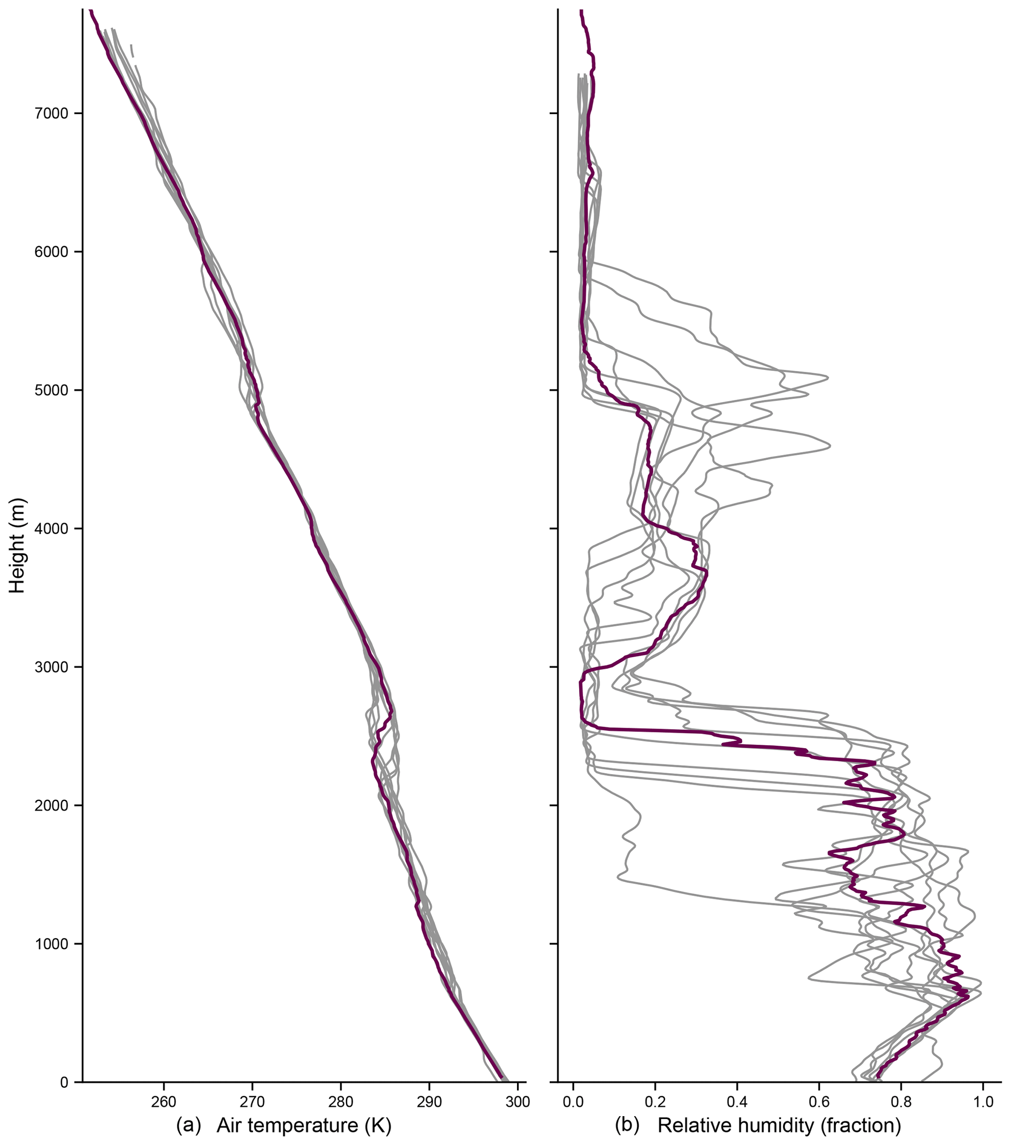
Figure 8 Profiles of air temperature (a) and relative humidity with respect to liquid (b) as obtained by dropsondes deployed from the P-3 (grey) and a radiosonde launched from the Ronald H. Brown (dark red). Dropsonde data are obtained from JOANNE (see text); radiosonde observations are obtained from the dataset described in Stephan et al. (2021). One of the 12 sondes shows much lower humidity from 1.5–2.5 km than do the others; we are assessing all the dropsonde circles to understand if this is common or an instrumental artifact.

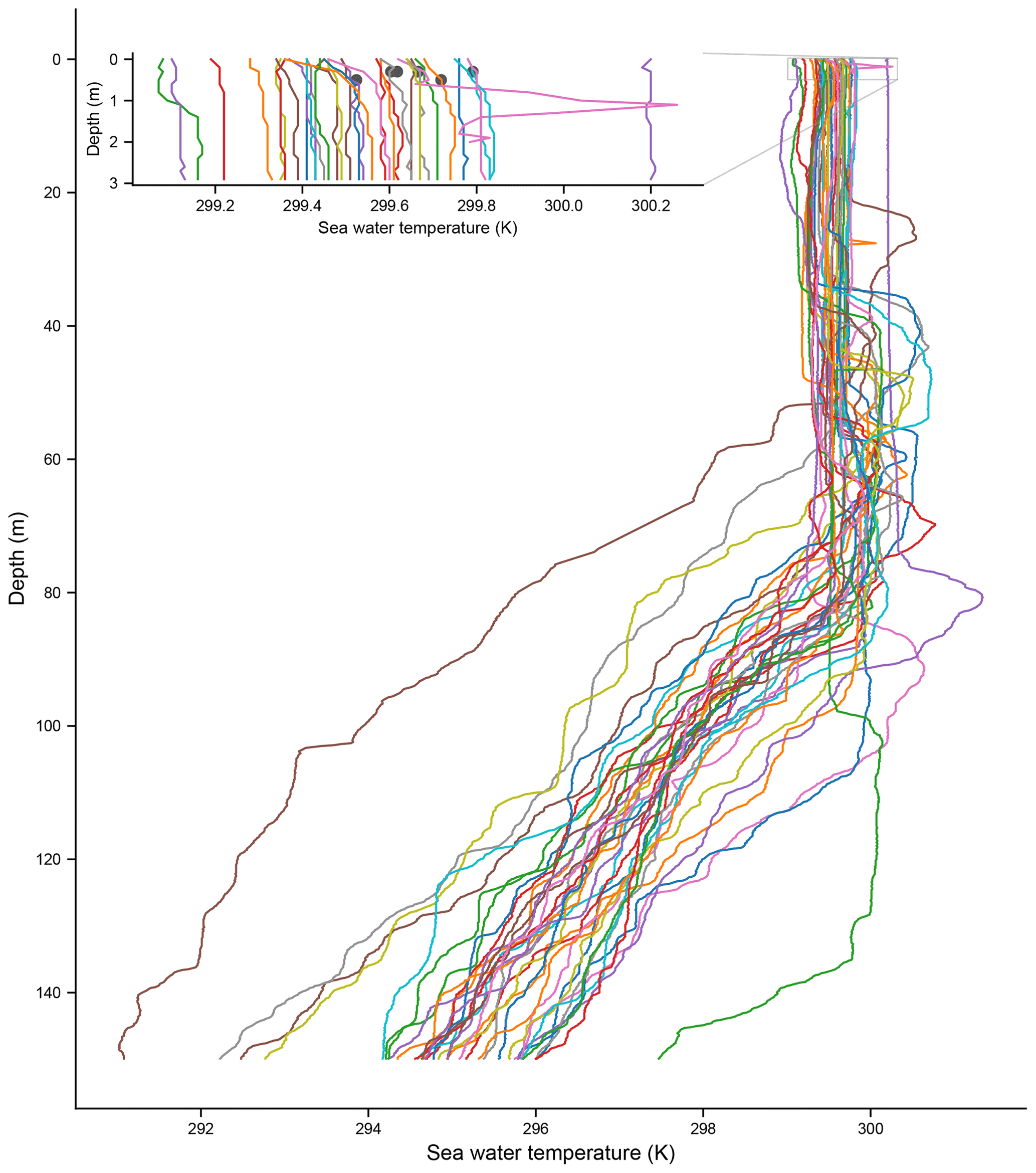
Figure 9 Ocean temperature profiles as measured by AXBTs deployed from the P-3 on 19 January 2020. Data are shown between the near-surface and a depth of 150 m, though the actual profiles extend to nearly 1000 m depth. The inset shows ocean temperatures in the first few meters along with measurements from the five SWIFT buoys (see Quinn et al., 2021) surrounded by the AXBT deployments. Three of the 40 AXBTs deployed did not provide valid data.

4.2.2 AXBTs

Following the processing of dropsonde data for JOANNE we have produced a single file containing all AXBTs profiles obtained during the ATOMIC, interpolated to a standard depth grid at 0.1 m vertical resolution. Figure 9 shows an example from the flight on 19 January 2020 in which 40 AXBTs were deployed in a lawnmower pattern bracketing five Surface Wave Instrument Float with Tracking (SWIFT; see Thomson, 2012) buoys deployed from the R/V Ronald H. Brown (see the upper right corner of Fig. 5). Figure 9 shows the ocean temperature as measured by the AXBTs between the surface and 150 m depth, with a near-isothermal mixed layer extending tens of meters and the cooler ocean below 60–80 m. The inset compares the temperature in the first 3 m with measurements made by the SWIFT buoys (see Quinn et al., 2021), nominally at 0.3–0.5 m depth depending on the particular buoy. Upper ocean temperatures measured by the AXBTs span 1 K; the range across the SWIFTs, which were more geographically confined, is about a fifth of this. Submesoscale and mesoscale eddies, fronts, and filaments in the ocean contribute to localized temperature gradients within this region (see also Fig. 4 in Quinn et al., 2021).

4.3 Remote sensing

4.3.1 W-band radar and infrared radiometer: clouds, precipitation, and sea state

We use observations from the W-band radar (Sect. 3.3.1) to estimate ocean surface parameters and, in combination with measurements from the downward-looking infrared radiometer (Sect. 3.3.4), to provide estimates of cloud properties. Both sets of parameters are distributed with navigation data interpolated to the 2 Hz radar time base. The file also contains values of the 10 m SFMR wind speed, both as reported by the instrument and as corrected via linear regression using dropsonde winds as the reference.

Estimates of sea state and precipitation rate make use of the strong reflection of the W-band radar from the ocean surface. Following Fairall et al. (2018) we report the measured normalized radar cross section NRCS_m based on the observed reflectivity factor of the ocean surface dBZ_e(0)

$$\begin{array}{}\text{(1)}& \begin{array}{rl}{\text{NRCS}}_{\mathrm{m}}=& {\text{dBZ}}_e\left(\mathrm{0}\right)+\mathrm{10}{\log }_{\mathrm{10}}\left({\mathit{\pi }}^{\mathrm{5}}\left|K^{\mathrm{2}}\right|\mathit{\delta }R/{\mathit{\lambda }}^{\mathrm{4}}\right)\\ & -\mathrm{180}+{\text{dBZ}}_{\mathrm{attn}}.\end{array}\end{array}$$

For the PSL W-band with its 30 m range resolution, the second term on the right-hand side of Eq. (1) is 137.9, while the correction factor for attenuation by water vapor and oxygen is roughly dBZ_attn=4 for typical ATOMIC conditions with the aircraft at 3 km altitude. During ATOMIC the signal from the surface was strong enough to cause some saturation of the receiver, reducing the sensitivity the nearer the aircraft was to the surface. Values of NRCS_m have been further adjusted for this effect as a function of pressure; the correction is small for altitudes higher than 5 km but is as large as 8 dB at 1 km above sea level.

The back-scattered radar return from the ocean surface σ depends on both wind speed and viewing angle θ; this dependence can be exploited to estimate the mean square slope $\stackrel{\mathrm{‾}}{s^{\mathrm{2}}}$ of surface waves (satellite-borne radar scatterometer wind estimates exploit the same physics). The dependence is usually represented (Walsh et al., 1998; Li et al., 2005) as

$$\begin{array}{}\text{(2)}& \mathit{\sigma }={\displaystyle \frac{{\mathrm{\Gamma }}^{\mathrm{2}}}{\stackrel{\mathrm{‾}}{s^{\mathrm{2}}}\cdot {\cos }^{\mathrm{4}}\mathit{\theta }}}\exp \left({\displaystyle \frac{-{\tan }^{\mathrm{2}}\mathit{\theta }}{\stackrel{\mathrm{‾}}{s^{\mathrm{2}}}}}\right),\end{array}$$

where Γ² is a wavelength-dependent constant with value 0.32 at W-band radar frequencies and the theoretical or calculated normalized radar cross section NRCS_c=10log ₁₀(σ). We solve Eq. (2) for $\stackrel{\mathrm{‾}}{s^{\mathrm{2}}}$, using observations made a nadir-viewing angles (θ=0) and assuming NRCS_c=NRCS_m. These estimates rely on radar calibration.

Following Fairall et al. (2018) the precipitation rate is determined from the W-band radar using the vertical gradient of radar reflectivity during light rain and the path-integrated attenuation during the infrequent heavy rain observed during ATOMIC.

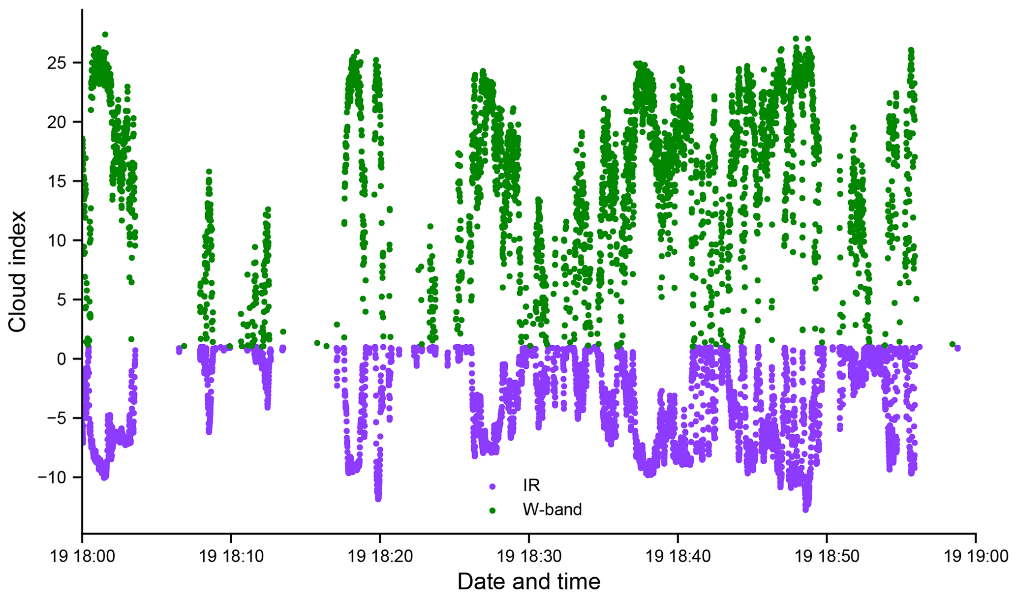
Figure 10 Cloud indexes based on radar (C^radar, green) and infrared radiometer (C^IR, purple) measurements for the period 18:00–19:00 UTC on 19 January (cf. Fig. 6). Cloud is indicated by values of C^radar>0 and C^IR<0. Absolute values less than one have been removed for clarity. The two indexes are quite consistent with one another because clouds, when present, are typically opaque enough to be easily detectable in both infrared and microwave measurements.

Clouds are detectable in both the radar reflectivity profile and the observed infrared brightness temperature. A radar cloud presence index C^radar is determined by examining the maximum signal-to-noise ratio (SNR) within each radar column (excluding the surface return). The clear-sky signal-to-noise level of the radar is nominally −20 dB, but a value of about −15 is needed to ensure a valid cloud return. We define the index as $C^{\mathrm{radar}}=max\left(\text{SNR}\right)+\mathrm{14}$ so that values of C^radar>0 indicate clouds. When clouds are detected cloud-top height z_ct is estimated as the level closest to the aircraft at which SNR>14. Cloud-top height diagnosed in this way is shown in the middle panel of Fig. 6. We report the radar reflectivity factor and Doppler velocity at this height as well as the wind speed w(z_ct) and air temperature T(z_ct as determined from daily-mean in situ aircraft profiles (not dropsondes).

An infrared cloud presence index C^IR is produced based on the observed nadir-looking brightness temperature T^IR(p) made at aircraft operating pressure p. We compare clear-sky measurements of T^IR(p) to the near-surface radiometric temperature, determined from the time mean of infrared radiometer measurements during flight legs at 150 m, to develop a correction term $\mathrm{\Delta }{T}^{\mathrm{IR}}(p-p{}^{\prime })=\text{SST}-T_{\mathrm{clear}}^{\mathrm{IR}}(p-p_{\mathrm{sfc}})$ as a quadratic function of $p-p{}^{\prime }$. The infrared cloud index C^IR is defined as the difference between the observed infrared temperature and the value expected in the absence of clouds, i.e., $C^{\mathrm{IR}}=T^{\mathrm{IR}}\left(p\right)-(\text{SST}-\mathrm{\Delta }{T}^{\mathrm{IR}}(p-p_{\mathrm{sfc}}\left)\right)$, so that values of C^IR<0 indicate clouds.

The two cloud indexes complement one another. The W-band radar sensitivity is limited, and, particularly when the aircraft was transiting or dropping sondes at 7.5 km altitude (about a quarter of the total flight time), many clouds near the surface were beyond the viewing range of the radar and are therefore not detectable in the radar return. For these flight legs the IR cloud index is likely a better indicator of cloudiness. When the aircraft is at or below about 3 km, the radar is very sensitive to clouds and likely detects all clouds with radar reflectivity factor $Z_e>-\mathrm{35}$ dBZ. Under these circumstances the radar and infrared cloud indexes are quite consistent with one another, as shown for an example hour of observations on 19 January 2020 in Fig. 10.

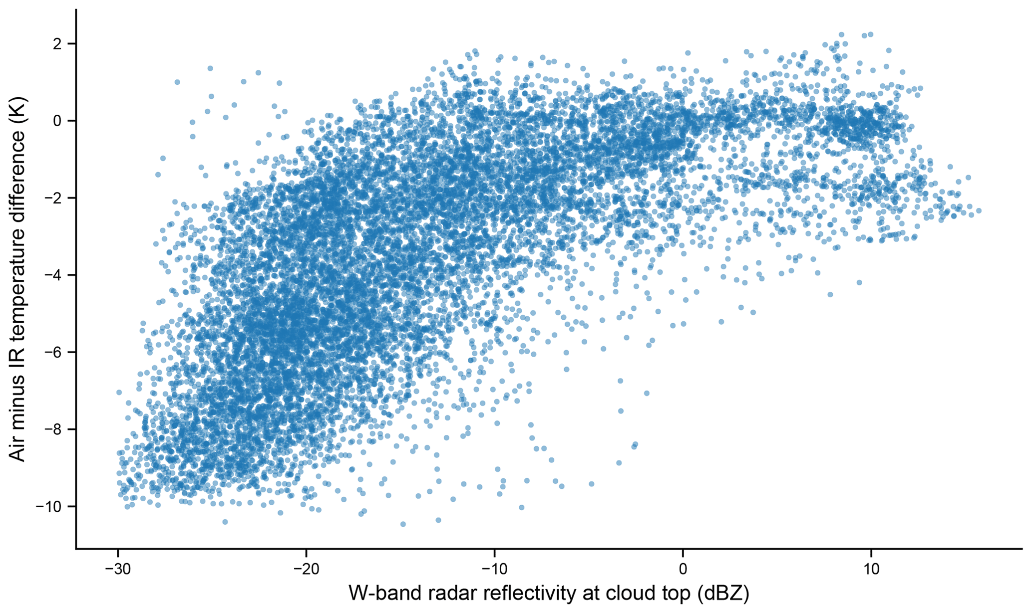
Figure 11 Difference between air temperature at cloud top $T_{\mathrm{ct}}^{\mathrm{air}}$ and the observed IR temperature $T_{\mathrm{ct}}^{\mathrm{IR}}$ as a function of W-band radar reflectivity at cloud top for the entire flight made on 19 January 2020. The height of the cloud top is determined as the closest position to the observing aircraft at which the radar signal-to-noise ratio exceeds 14 dB; air temperature as a function of height is determined from in situ samples made by the aircraft. Temperature differences near zero indicate that the clouds are optically thick in the infrared.

When cloud-top height z_ct is available from the radar we use this information to identify cloud-top pressure p_ct and, from aircraft soundings, the temperature at that pressure $T_{\mathrm{ct}}^{\mathrm{air}}$. This can be compared to IR cloud-top temperature corrected for the intervening atmosphere $T_{\mathrm{ct}}^{\mathrm{IR}}=T^{\mathrm{IR}}\left(p\right)+\mathrm{\Delta }{T}^{\mathrm{IR}}(p-p_{\mathrm{ct}})$. Values of $T_{\mathrm{ct}}^{\mathrm{IR}}\approx T_{\mathrm{ct}}^{\mathrm{air}}$ indicate that optically thick clouds fill the infrared radiometer's field of view. In Fig. 11 we show the difference in cloud-top air temperature and apparent IR cloud-top temperature as a function of W-band reflectivity from 19 January. Values of $T_{\mathrm{ct}}^{\mathrm{IR}}-T_{\mathrm{ct}}^{\mathrm{air}}$ less than zero indicate the cloud is optically thin or does not completely fill the 0.5 s sample and some radiation from the warm sea surface is adding to the measured IR.

Figure 12 Observations of surface wave state from the Wide Swath Radar Altimeter (WSRA) during the P-3 flight of 19 January 2020. (a) Mean square slope (rad²). (b) Significant wave height (m).

4.3.2 WSRA: sea state and rain rate information

ProSensing Inc. processes raw data from the Wide Swath Radar Altimeter (WSRA; see Sect. 3.3.2) to produce information about the wave state of the ocean surface. Most observations – including the power spectrum of surface waves as a function of wavenumber in the north–south and east–west directions; the direction, height, and wavelength of the two most dominant waves; peak spectral variance; and the significant wave height – are reported every 50 s. A plan view of observations obtained on 19 January 2020 is shown in Fig. 12. Rainfall rate and surface wave $\stackrel{\mathrm{‾}}{s^{\mathrm{2}}}$ are reported every 10 s. The latter is computed from the decrease in the intensity of the return with scan angle following Eq. (2), so, unlike estimates of $\stackrel{\mathrm{‾}}{s^{\mathrm{2}}}$ from the W-band radar, estimates from the WSRA do not depend on absolute calibration.

Files with these estimates also contain bookkeeping information (processing parameters and ancillary data) such as aircraft navigation and orientation and other fields that may be useful. In particular, the directional wave spectra calculated from data collected with WSRA inherently contain a 180^∘ ambiguity of the wave propagation which can generally be eliminated using a rough estimate of a predicted dominant ocean wave direction at the location of the observation point. During ATOMIC the prevailing wind direction (typically ENE to WSW) was used as the predicted ocean wave direction for the entire duration of each flight mission. For completeness WSRA files contain directional wave spectra with and without this ambiguity removed.

During ATOMIC the aircraft operated in a number of modes that were unfavorable for collecting WSRA data. Data should not be used if the aircraft altitude is less than 500 m or greater than 4000 m, or when the aircraft's pitch or roll exceeds ±3^∘. We also recommend using observations only when the peak spectral value is in the range 0.0002–0.006 m².

5 Code and data availability

Data have been reformatted into netCDF files following CF (Climate and Forecast) conventions (https://cfconventions.org, last access: 11 June 2021), which provide for units and standard names for variables, a uniform handling of time, and other metadata intended to promote interoperability and interpretability. The files also contain some provenance information following guidance developed for EUREC⁴A. Isotope ratios from the isotope analyzer aboard the P-3 (Sect. 3.1.2) will be described as part of a paper describing the aircraft-, ship-, and ground-based observations made during the experiments.

Data have been archived at NOAA's National Center for Environmental Information as detailed in Table 4. This represents the version of record. The data are also replicated at the French AERIS data center alongside the wide array of other data from the EUREC⁴A experiment (OPeNDAP access via https://observations.ipsl.fr/thredds/catalog/EUREC4A/catalog.html, last access: 11 June 2021).

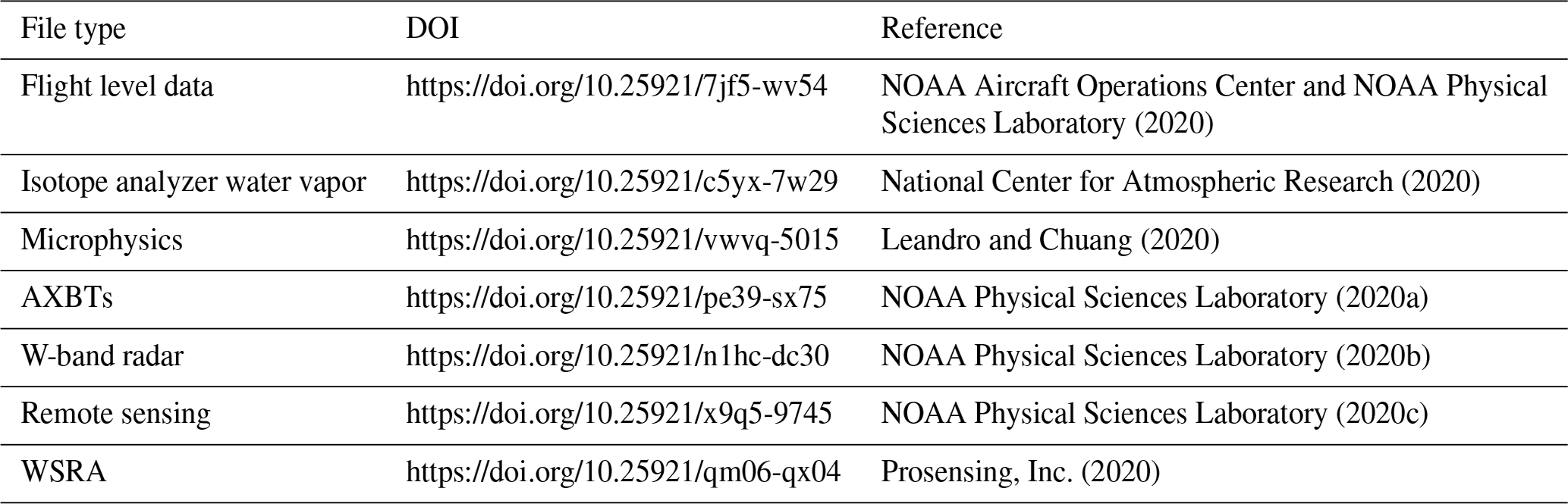
2020National Center for Atmospheric Research (2020)Leandro and Chuang (2020)NOAA Physical Sciences Laboratory (2020a)NOAA Physical Sciences Laboratory (2020b)NOAA Physical Sciences Laboratory (2020c)Prosensing, Inc. (2020)

Table 4 Data described in this paper and archived at NOAA's National Center for Environmental Information. The contents of each file are summarized in Table 3; document object identifiers (DOIs) point to netCDF files following Climate and Forecast conventions.

6 Conclusions

Measurements from the P-3 during ATOMIC took place in the context of marine measurements in the remote ocean (Quinn et al., 2021) and autonomous airborne measurements made from the island of Barbados (de Boer et al., 2021), all aimed at understanding how mesoscale structures in the atmosphere and ocean affect the coupling between the two components of the earth system. The measurements exist in the wider context of EUREC4A (Stevens et al., 2021) and, in aggregate, provide an unprecedented look at the tropical atmosphere, the shallow clouds embedded in it, and the ocean as a coupled system.