the Creative Commons Attribution 4.0 License.
the Creative Commons Attribution 4.0 License.
 | 27 Apr 2021
Gap-free global annual soil moisture: 15 km grids for 1991–2018
Mario Guevara
Michela Taufer
Soil moisture is key for understanding soil–plant–atmosphere interactions. We provide a soil moisture pattern recognition framework to increase the spatial resolution and fill gaps of the ESA-CCI (European Space Agency Climate Change Initiative v4.5) soil moisture dataset, which contains > 40 years of satellite soil moisture global grids with a spatial resolution of ∼ 27 km. We use terrain parameters coupled with bioclimatic and soil type information to predict finer-grained (i.e., downscaled) satellite soil moisture. We assess the impact of terrain parameters on the prediction accuracy by cross-validating downscaled soil moisture with and without the support of bioclimatic and soil type information. The outcome is a dataset of gap-free global mean annual soil moisture predictions and associated prediction variances for 28 years (1991–2018) across 15 km grids. We use independent in situ records from the International Soil Moisture Network (ISMN, 987 stations) and in situ precipitation records (171 additional stations) only for evaluating the new dataset. Cross-validated correlation between observed and predicted soil moisture values varies from r= 0.69 to r= 0.87 with root mean squared errors (RMSEs, m3 m−3) around 0.03 and 0.04. Our soil moisture predictions improve (a) the correlation with the ISMN (when compared with the original ESA-CCI dataset) from r= 0.30 (RMSE = 0.09, unbiased RMSE (ubRMSE) = 0.37) to r= 0.66 (RMSE = 0.05, ubRMSE = 0.18) and (b) the correlation with local precipitation records across boreal (from r= < 0.3 up to r= 0.49) or tropical areas (from r= < 0.3 to r= 0.46) which are currently poorly represented in the ISMN. Temporal trends show a decline of global annual soil moisture using (a) data from the ISMN ( %), (b) associated locations from the original ESA-CCI dataset ( %), (c) associated locations from predictions based on terrain parameters ( %), and (d) associated locations from predictions including bioclimatic and soil type information ( %). We provide a new soil moisture dataset that has no gaps and higher granularity together with validation methods and a modeling approach that can be applied worldwide (Guevara et al., 2020, https://doi.org/10.4211/hs.9f981ae4e68b4f529cdd7a5c9013e27e).
- Article
(7160 KB) - Full-text XML
- BibTeX
- EndNote


Soil moisture data are essential for scientific inquiry in a variety of research areas. These data enable scientists to characterize hydrological patterns (Greve and Seneviratne, 2015), quantify the influence of soil moisture on terrestrial carbon dynamics (van der Molen et al., 2011), identify trends in global climate variability (Seneviratne et al., 2013), analyze the response of ecosystems to moisture decline (Zhou et al., 2014), or detect the impact of moisture on models of land–atmosphere interactions (May et al., 2016). The integrity of current soil moisture data is fundamental for a comprehensive understanding of the global water cycle (Al-Yaari et al., 2019).
The main sources of soil moisture data are in situ soil moisture measurements through monitoring networks such as the International Soil Moisture Network (ISMN; Dorigo et al., 2011a) and satellite soil moisture measurements such as those provided by the European Space Agency Climate Change Initiative (ESA-CCI; Dorigo et al., 2017; Liu et al., 2011). Both measurement techniques can quantify regional-to-continental global soil moisture patterns and dynamics (Gruber et al., 2020).
In situ soil moisture measurements assess soil moisture within specific study sites at specific soil depths (e.g., 0–5 cm). These measurements are fine-grained as soil moisture sensors have a small and localized footprint, and despite national and international networks they are limited in much of the world (Fig. 1). Collection of in situ soil moisture data across large areas is expensive and time consuming; in many cases, logistical challenges such as limited funding for data collection and accessibility of soil moisture monitoring sites make it impossible.
On the other hand, satellite soil moisture measurements collected in the form of microwave radiometry using L band (∼ 1.4–1.427 GHz) and C band (∼ 4–8 GHz) are more effective for larger regional-to-global soil moisture measurements (Mohanty et al., 2017). As for most available in situ soil moisture measurements, satellite soil moisture datasets are representative for the first 0–5 cm of soil depth. Unlike the fine-grained in situ measurements, satellite soil moisture datasets are available at the global scale in coarse-grained grids with spatial resolution ranging between 9 and 25 km (Senanayake et al., 2019) and at the regional scale (e.g., the European continent) with a spatial resolution of 3 km grids (Naz et al., 2020). A well-known satellite soil moisture dataset is collected by ESA-CCI. The ESA-CCI dataset contains more than 40 years of satellite soil moisture global grids (from 1978 to 2019) with a spatial resolution of ∼ 27 km (Liu et al., 2011; Chung et al., 2018). This soil moisture dataset is a synthesis from multiple soil moisture sources and has been applied in long-term ecological and hydrological studies (Dorigo et al., 2017). The dataset covers a longer period of time compared with other satellite-derived soil moisture datasets (e.g., Soil Moisture Active Passive (Al-Yaari et al., 2019).
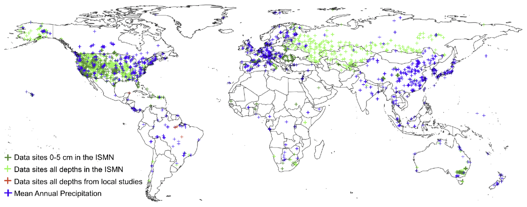
Figure 1Spatial distribution of available data from in situ monitoring sites. This information was only used for validating our soil moisture predictions. The ISMN (green for all data sites and dark green for sites with available information at 0–5 cm), precipitation records (blue), and soil moisture additional datasets from previous local studies (red).
Across large areas of the world, the ESA-CCI soil moisture data have been validated and calibrated against in situ soil moisture measurements (Al-Yaari et al., 2019; Dorigo et al., 2011a). In addition, there are continuing efforts to improve the spatial reliability of the satellite measurements (Gruber et al., 2017), resulting in new dataset versions. However, even the most recent versions of ESA-CCI soil moisture data (i.e., v4.5 to 5.0) still suffer from a too-coarse-grained spatial resolution and substantial spatial gaps in their spatial coverage (Llamas et al., 2020), making the data unsuitable to tackle problems such as quantifying the implications of soil moisture in water cycle across fine-grained scales or across areas with spatial gaps. Scientists have developed empirical and physical modeling approaches for predicting missing satellite soil moisture data (Peng et al., 2017; Sabaghy et al., 2020) and for evaluating the errors in soil moisture satellite model predictions (Gruber et al., 2020). The spatial resolution and coverage of these recent studies are still an emergent challenge due to limited data across large areas of the world (e.g., extremely dry, extremely wet, or frozen regions) as well as the signal excessive noise and saturation affecting the quality of satellite soil moisture records. Consequently, there is a need for developing alternative modeling approaches and their validation methods to fill the gaps of the ESA-CCI dataset, improving both the spatial resolution and the coverage. Recent soil moisture products across Europe and the United States (Bauer-Marschallinger et al., 2018, Guevara and Vargas, 2019) reveal the possibility of developing high-spatial-resolution surface soil moisture estimates that complement the coarse spatial granularity of available remote sensing products (e.g., ESA-CCI).
In this study we tackle the need to increase spatial granularity and provide gap-free global soil moisture predictions. In doing so, we combine a pattern recognition technique called kernel-weighted k-nearest neighbors (or k-KNN; Hechenbichler and Schliep, 2004) with the use of independent covariate or prediction factors such as topographic parameters, bioclimatic features, and soil types. Our approach enables us to augment both spatial resolution and coverage in the ESA-CCI dataset despite limited data in large areas of the world.
k-KNN is a machine learning (ML) algorithm that has several benefits for predicting satellite soil moisture at the global scale. First of all, k-KNN accounts for non-linearities (e.g., local and regionally specific data patterns). Soil moisture data (as a dependent variable) can be predicted as a function of the spatial variability of environmental data (independent variables) with different spatial resolution and coverage (Peng et al., 2017; Guevara and Vargas, 2019; Llamas et al., 2020). k-KNN can take advantage of the spatial autocorrelation of training data such as the relation between variance and distance between soil moisture observations (Llamas et al., 2020; Oliver and Webster, 2015) and use it as ancillary information when spatial coordinates (e.g., latitude and longitude) are considered in the prediction approach (Hengl et al., 2018; Behrens et al., 2018; McBratney et al., 2003). Second, k-KNN can use kernel functions to weight the neighbors according to their distances. Finally, by including spatial coordinates in the predictions, k-KNN can consider geographical distances. In doing so, it is able to account for local and regional variability in the feature space: each predicted value is dependent on a unique combination of k neighbors in the feature space that are weighted using kernel functions that can be different from one place to another (see Sect. 2.2).
We use a diverse set of independent covariates or prediction factors such as topographic parameters, bioclimatic features, and soil types to augment the prediction of soil moisture values with k-KNN. Topographic parameters are based on physical principles related to the overall distribution of surface water across the landscape (Western et al., 2002; Moeslund et al., 2013; Mason et al., 2016). We generate the topographic parameters from digital terrain analysis. Digital terrain analysis involves calculations of land surface characteristics that depend on topography (e.g., terrain slope and aspect; Wilson, 2012). The impact of terrain parameters on spatial variability of satellite soil moisture is supported by previous studies that have provided evidence of a topographic signal in satellite soil moisture measurements from local (Mason et al., 2016) to continental scales (Guevara and Vargas, 2019). Other studies derive terrain parameters from elevation data and use them to predict soil moisture across a gradient of hydrological conditions (Western et al., 2002). Topographic parameters have also been used for soil attribute predictions (Moore et al., 1993) and for soil moisture mapping applications (Florinsky, 2016). All these studies suggest that topography (represented by multiple terrain parameters) is a useful predictor of surface soil moisture variability at the global scale. Different types of terrain parameters exist, including elevation data structures, topographic wetness, overland flow, and potential incoming solar radiation, among others. Elevation data structures (i.e., point elevation data, elevation contour lines, or digital elevation models) quantitatively represent topographic variability and are the basis of digital terrain analysis (i.e., geomorphometry). The topographic wetness index is a terrain parameter that characterizes areas where soil moisture increases by the effect of overland flow accumulation (Moore et al., 1993). Overland flow and potential incoming solar radiation are two important topographic drivers of the spatial distribution of soil moisture (Nicolai-Shaw et al., 2015), its lags after precipitation events (McColl et al., 2017), and its role as a dominant control of plant productivity (Forkel et al., 2015). Bioclimatic features and soil types account for hydroclimatic and soil variability affecting soil moisture. We add bioclimatic features and soil type classes as additional prediction factors to our approach to determine if information beyond terrain parameters substantially improves soil moisture predictions. To validate our dataset, we use independent in situ information (i.e., annual soil moisture measurements) from local studies (n= 8 stations; Vargas, 2012; Saleska et al., 2013), from the ISMN (n= 2185 stations), and from precipitation records across the world (n= 171 stations, including tropical areas poorly represented in the ISMN).
The contributions of this paper are 2-fold: first, we integrate the k-KNN algorithm and prediction factors into a modeling approach to predict fine-grained, gap-free soil moisture data with a resolution of 15 km; second, we generate a new dataset that complements the ESA-CCI dataset and is composed of soil moisture predictions from our modeling approach. With reference to our first contribution, we study the effectiveness of k-KNN in downscaling satellite-derived soil moisture using two prediction factor datasets: a first dataset based only on topographic parameters and a second based on topographic parameters, bioclimatic features, and soil types. We compare the accuracy of the two types of fine-grained, gap-free soil moisture models obtained using the two prediction factor datasets. The comparison allows us to assess the impact of the individual prediction factors. Specifically, we address the impact of topographic parameters versus bioclimatic features and soil types. Previous studies have used a variety of prediction factors for soil moisture, including vegetation indexes (from optical imagery), climate information (Alemohammad et al., 2018), choropleth maps (i.e., land use and land forms), thermal data, and soil information to improve the spatial resolution and coverage of soil moisture gridded datasets (Naz et al., 2020; Peng et al., 2017). In contrast to past efforts, our solution uses a comprehensive set of factors for predicting satellite soil moisture data and independently testing the model with in situ soil moisture data. Our approach is computationally less expensive and prevents potential spurious correlations when predicted soil moisture estimates are compared with climate, vegetation, or soil information. With reference to our second contribution, we generate a dataset complementary to the ESA-CCI soil moisture dataset that provides gap-free global mean annual soil moisture predictions for 28 years (1991–2018) across a 15 km grid (note that ESA-CCI has a grid of 27 km). Our soil moisture dataset can be used for identifying spatial and temporal patterns of soil moisture and its contributions to climate and vegetation feedbacks. The soil moisture predictions, the field soil moisture validation dataset, and the set of prediction factors for soil moisture are publicly available (Guevara et al., 2020).
Our prediction approach has four key steps. First, we define training soil moisture datasets and define two different datasets of prediction factors with a 15 km global grid resolution: a dataset consisting only of terrain parameters and a different dataset combining terrain parameters, bioclimatic features, and soil type classes (Sect. 2.1). Second, we build prediction models by feeding the prediction factors and ESA-CCI satellite soil moisture data to the k-KNN algorithm and using cross-validation for selecting the best models (Sect. 2.2). Third, we bootstrap the parameters to assess variances of soil moisture predictions (Sect. 2.3). Last, we validate our best predictions against independent in situ soil moisture measurements when they are available (Sect. 2.4).
2.1 Training datasets and datasets of prediction factors
We generate a training dataset for each analyzed year (n= 28). A training dataset consists of a table with the central coordinates of each pixel in the ESA-CCI dataset and the corresponding satellite-derived soil moisture values for a given year. We use all available pixels with valid soil moisture values reported in the ESA-CCI v4.5 and calculate (for each pixel) the mean value of all available observations for a given year. We do not consider a threshold value (e.g., a minimum number of pixels) to calculate the mean for each pixel for a given year. There are large areas in the world (mainly in the tropics or deserts) with missing information throughout an entire year. After identifying the gaps for each year, we observe that the years with the largest number of missing values (i.e., data not available; NAs) are between years 2003 and 2006 (Appendix A, Fig. A1).
We generate and test two different datasets of prediction factors with a 15 km grid resolution: (a) a dataset of only digital terrain parameters and (b) a more complex dataset that uses digital terrain parameters, static bioclimatic features, and soil type information. The second dataset allows us to differentiate between the impact of terrain parameters in isolation and the impact of terrain parameters when augmented with static bioclimatic features and soil type information. The values of prediction factors are generated to overlap with the central coordinates (latitude and longitude) of the original ESA-CCI soil moisture pixels following previous research (Guevara and Vargas, 2019).
Digital terrain parameters (described in Fig. 2) are derived from a global digital elevation model using SAGA-GIS (System for Automated Geoscientific Analysis GIS) (Conrad et al., 2015). The source of elevation data is a radar-based digital elevation model (Becker et al., 2009). This digital elevation model is provided by Hengl et al. (2017), and we re-sampled it (along with bioclimatic features and soil type classes) to a spatial resolution of 15 km grids across the world. We consider the following terrain parameters: (a) terrain aspect (aspect), (b) specific catchment area (carea), (c) channel network base level (chnl base), (d) distance to channel network (chnl dist), (e) flow convergence index (convergence), (f) horizontal curvature (hcurv), (g) digital elevation model (land), (h) length–slope factor (lsfactor), (i) relative slope position (rsp), (j) analytical hillshade (shade), (k) smoothed elevation (sinks), (l) terrain slope (slope), (m) valley depth index (vall depth), (n) vertical curvature (vcurv), and (o) topographic wetness index (wetness). The parameters are presented in Fig. 2, and a detailed description and units of the parameters can be found in Guevara and Vargas (2019).
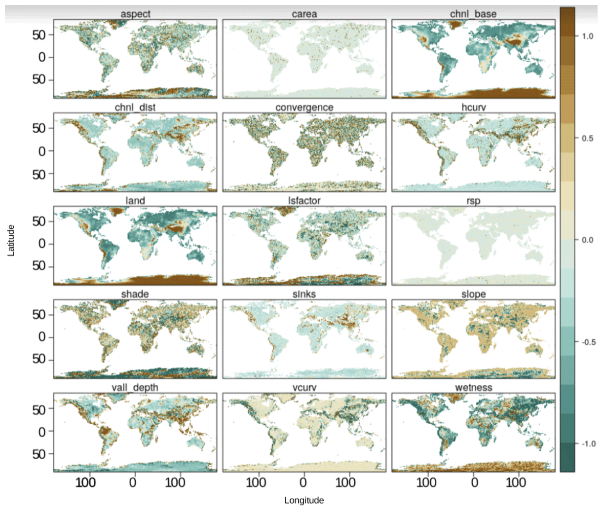
Figure 2Digital terrain parameters used as prediction factors for soil moisture. These parameters are derived from a digital elevation model using SAGA-GIS. These terrain parameters are standardized by centering their means to zero and a variance unit for visualization purposes. Legend: (a) terrain aspect (aspect), (b) specific catchment area (carea), (c) channel network base level (chnl base), (d) distance to channel network (chnl dist), (e) flow convergence index (convergence), (f) horizontal curvature (hcurv), (g) digital elevation model (land), (h) length–slope factor (lsfactor), (i) relative slope position (rsp), (j) analytical hillshade (shade), (k) smoothed elevation (sinks), (l) terrain slope (slope), (m) valley depth index (vall depth), (n) vertical curvature (vcurv), and (o) topographic wetness index (wetness). For a detailed description and units of these parameters see Guevara and Vargas (2019).
Static bioclimatic features are extracted from the Food and Agriculture Organization Global Agro-Ecological Zones project (FAO, 2013; baseline period: 1961–1990) to account for hydroclimatic variability. Thus, these static bioclimatic features consist of a spatial database of land mapping units with the following categories: (1) boreal coniferous forest, (2) boreal mountain system, (3) boreal tundra woodland, (4) polar, (5) subtropical desert, (6) subtropical dry forest, (7) subtropical humid forest, (8) subtropical mountain system, (9) subtropical steppe, (10) temperate continental forest, (11) temperate desert, (12) temperate mountain system, (13) temperate oceanic forest, (14) temperate steppe, (15) tropical desert, (16) tropical dry forest, (17) tropical moist deciduous forest, (18) tropical mountain system, (19) tropical rain forest, and (20) tropical shrubland.
These categories were developed for assessing global land resources following a methodology has been jointly developed by FAO and the International Institute for Applied Systems Analysis (Fischer et al., 2000). Each category is expressed within independent maps of zeros and ones (absence and presence, respectively, at each pixel), and this information is considered as an independent quantitative predictor.
As soil type information, we include soil water retention capacity classes (1: 150 mm water per meter of the soil unit; 2: 125 mm; 3: 100 mm; 4: 75 mm; 5: 50 mm; 6: 15 mm; 7: 0 mm) from the Regridded Harmonized World Soil Database v1.2 (Wieder et al., 2014) to account for soil type variability in our prediction framework. In this soil type map the distance between the above-mentioned water retention classes is known (e.g., from high to low every 25 mm of water), and it can be considered a quantitative predictor.
For each pixel with available soil moisture values in the ESA-CCI dataset, we augment the spatial coordinates (i.e., latitude and longitude) and soil moisture value by adding the tuple of the 15 terrain parameters for the first dataset and the tuple of the 15 terrain parameters, the 19 bioclimatic features, and the soil type classes for the second dataset. The pixels without soil moisture values become our prediction targets. Because the prediction factor datasets have a 15 km resolution while the ESA-CCI soil moisture pixels have a 27 km resolution, we preprocess each prediction factor dataset to extract the values to the corresponding locations of the ESA-CCI pixels. By overlapping the original ESA-CCI dataset with one of the two prediction factor datasets and extracting the prediction factor values for the ESA-CCI pixel centers, we generate two augmented ESA-CCI datasets. A similar method was initially used for the conterminous United States (Guevara and Vargas, 2019), and here we extend the method to the entire world. In our mapping, we leverage observations from other work outlining the positive impact of spatial structure (e.g., spatial distances and autocorrelation) on soil attribute predictions (e.g., soil moisture) (see spatial coordinate maps in Fig. A1) (Llamas et al., 2020; Møller et al., 2020; Hengl et al., 2018; Behrens et al., 2018; McBratney et al., 2003; Oliver and Webster, 2015). We include spatial coordinates in our modeling framework (described in Sect. 2.2) to account for the spatial structure of the ESA-CCI training data. To this end, we use spatial coordinates at multiple oblique angles as suggested by recent work (Møller et al., 2020, Appendix A, Fig. A2). This preprocessing is done using open-source R software functionalities for geographical information systems (R Core Team, 2020; Hijmans, 2019).
2.2 Building prediction models
To build prediction models of the soil moisture at a finer spatial resolution (15 km) than the original ESA-CCI dataset (27 km), we use the kernel-based method for pattern recognition known as k-KNN (Hechenbichler and Schliep, 2004). We build one model per year (n= 28 models). We observe that the relationships among spatial coordinates, soil moisture values, terrain parameters, bioclimatic classes, and soil types are not linear. For example, south slope areas tend to be dryer than north slopes areas. Moreover, there is a contrasting feedback of soil moisture and precipitation between humid and dry areas (e.g., between the eastern and western United States; Tuttle and Salvucci, 2016). We use k-KNN because it allows us to account for the non-linear feedback while providing a simple and fast prediction solution.
The k-KNN algorithm has two main settings: (a) the parameter k that determines the number of neighbors from which information is considered for prediction and (b) a kernel function that converts distances among neighbors into weights, so the farther the neighbor, the smaller the weight it will be assigned. We consider k neighbors with k ranging from 2 to 50 soil moisture pixels and with close spatial coordinates and similar prediction factors. In the case of the first prediction factor dataset (i.e., only digital terrain parameters), distances among neighbors are computed among spatial coordinates and terrain parameters; in the case of the second dataset (i.e., digital terrain parameters, static bioclimatic features, and soil type classes), distances among neighbors are computed among spatial coordinates, terrain parameters, static bioclimatic features, and soil type classes. The similarity among neighbors is measured with the Minkowski distance (i.e., the statistical average of the neighbors' value difference). We consider six different kernel functions (i.e., rectangular, triangular, Epanechnikov, Gaussian, rank, and optimal).
Using the two augmented ESA-CCI datasets obtained by overlapping the original ESA-CCI dataset with one of the two prediction factor datasets and extracting the prediction factor values for the ESA-CCI pixel centers (from Sect. 2.1), we generate two sets of 28 prediction models, one for each of the 28 years (i.e., 1991–2018) in the ESA-CCI soil moisture dataset (v4.5). We feed the augmented ESA-CCI datasets into the k-KNN algorithm and search for the most effective k neighbors' values and kernel functions. To this end, we use 10-fold cross-validation to select the values of the k neighbors among the 48 possible values (i.e., k ranged from 2 to 50) and the kernel function from these six kernel functions (i.e., rectangular, triangular, Epanechnikov, Gaussian, rank, and optimal). We use cross-validation as a re-sampling technique because it can prevent overfitting in ML methods such as k-KNN and can generate multiple sets of independent model residuals to evaluate the stability of prediction outcomes. The use of cross-validation for searching for the most effective k neighbors' values and kernel function requires us to randomly create multiple independent training and testing datasets. Training and testing datasets generated from one of our augmented ESA-CCI datasets are disjoined; training data are used for building the models, and testing data are used only for quantifying model residuals and evaluating soil moisture predictions.
As our cross-validation indicators (i.e., information criteria about prediction), we use the Pearson correlation coefficient (r) and the root mean squared error (RMSE) for each one of the prediction models. For each year we select the model whose combination of k and kernel function has the highest r and lowest RMSE. We use the model to predict annual mean global soil moisture across 15 km global grids.
2.3 Assessing variances of model predictions
We study three sources of modeling variance. First, we assess the sensitivity of the prediction models to variations in available training data over the entire world. Second, we assess the relevance of the spatial coordinates and different prediction factors by rebuilding the models using the k-KNN algorithm with and without each prediction factor, once again over the entire world. Third, we assess the effectiveness of the k-KNN algorithm across selected areas of the world with fewer data available for training the prediction models and with different environmental and climate gradients.
To assess the sensitivity of the prediction models to variations in training data, we compute the variance of our soil moisture predictions as surrogates of model-based uncertainty. We rebuild the prediction models setting the k-KNN algorithm to use different random subsets of available pixels (n= 1000) and 10-fold repeated cross-validation (n= 10) to quantify the variance of soil moisture predictions. This model variance enables us to identify geographical areas with high or low sensitivity of prediction models to random variations in training data.
To assess the relevance of the different prediction factors, we use the r and RMSE of modeling with all prediction factors as a reference, and we compare the r and RMSE with the r and RMSE values of modeling without each one of the prediction factors. We test the sensitivity of the spatial coordinates and each prediction factor (i.e., terrain parameters, bioclimatic features, and soil type classes) by systematically leaving out one prediction factor at a time and repeating our k-KNN algorithm and its respective cross-validation. This process is repeated 10 times for each prediction factor to capture a variance estimate. This empirical validation approach provides empirical insights of the relative importance of prediction factors for the k-KNN algorithm predicting soil moisture at the global scale.
To assess the effectiveness of the k-KNN algorithm across specific areas of the world, we first test the k-KNN algorithm in tropical areas (Appendix A, Fig. A3) with low availability of data to train prediction models (e.g., greater distances between k neighbors) and under homogeneous environmental and climate conditions (e.g., higher water content above ground than below ground). We extract the limits of tropical areas from the Global Agro-Ecological Zones project (FAO, 2013; baseline period: 1961–1990; described in Sect. 2.1). Second, we test the k-KNN algorithm using only the available ESA-CCI data across countries with large heterogenous environmental and climate gradients, such as Canada, Australia, and Mexico. We generate new training, testing, and prediction factor datasets for these countries using geopolitical limits provided by the Global Administrative Areas (GADM, 2021). We use the resulting model predictions to explore modeling consistency in terms of r and RMSE values across the selected areas and to visualize spatial patterns between the ESA-CCI soil moisture dataset and our soil moisture predictions.
2.4 Validation against independent in situ data
We validate the ESA-CCI dataset and our predictions against in situ soil moisture data reported in ISMN for each year. Additionally, we compare soil moisture trends (i.e., changes in soil moisture over time) by comparing either in situ soil moisture or the ESA-CCI with our predictions.
We first augment the original ISMN (downloaded in August of 2019) from the datasets with information from eight stations with in situ soil moisture data from literature reviews that are distributed in open-access data repositories: one station was deployed in a tropical forest of Mexico with data from 2006 to 2008 (Vargas, 2012), and seven stations across Brazil's tropical forests with data from 1999 to 2006 (Saleska et al., 2013).
To perform the validation, we compute yearly means at every available location of the ISMN dataset. Then, we organize for further comparisons these yearly means with the yearly means of the combined ESA-CCI (v4.5) soil moisture grids and our soil moisture predictions. Consequently, further analyses are consistent in space (i.e., locations from the ISMN and corresponding pixels in the ESA-CCI (v4.5) and our predictions) and time (1991–2018). We first calculate the yearly means using all available soil moisture values per site in the ISMN (n= 2185 stations), and then we extract the sites containing information of soil moisture for the 0–5 cm for further analyses (n= 987 stations, 1996–2016).
To complement our validation strategy, we perform an additional independent validation against in situ records of annual precipitation (n= 171 stations). This information was extracted from the global soil respiration database (Bond-Lamberty and Thomson, 2018) and represented the years 2008 to 2018. Soil moisture and precipitation are closely related variables (McColl et al., 2017), and previous work has recommended the use of soil-moisture-related information to validate soil moisture predictions in the absence of in situ soil moisture information (Gruber et al., 2020). The purpose of including precipitation datasets is to enrich the spatial representation of soil-moisture-related information for comparative purposes between the ESA-CCI and our soil moisture predictions.
We highlight that any potential bias associated with the data in our augmented ISMN dataset (e.g., stations with low number of records) has potentially the same impact on the validation results of the three datasets (ESA-CCI and our two prediction datasets). In other words, we assume biases are randomly distributed across all observations, and thus they are not accounted for in the outcome of our comparisons. We summarize the validation results in a target diagram to illustrate the accuracy of our soil moisture predictions. The target diagram (presented in Appendix A, Fig. A4; Jolliff et al., 2009) shows the relation between the variance and magnitude of errors (i.e., unbiased root mean squared error, or ubRMSE) (a) between the ESA-CCI and the augmented ISMN dataset and (b) between our predictions and the augmented ISMN dataset.
To compare trends in soil moisture over time for areas for which we have in situ data, we perform a non-parametric (median-based) trend detection test (i.e., Theil–Sen estimator) to compare soil moisture trends at the locations of the augmented ISMN dataset. This trend detection is done by calculating the median value of the slopes and intercepts of all possible combinations of pairs of points in the relationship of soil moisture (response) and time (explanatory variable). This resulting median slope and intercept estimates are unbiased and resistant to outliers (Kunsch, 1989).
For those areas in which the ISMN dataset has multiple gaps, we rely on the ESA-CCI and our prediction datasets to generate a map of soil moisture trends. To this end, we apply a pixel-wise trend detection test to the ESA-CCI and prediction datasets to search for possible breakpoints (i.e., significant changes in soil moisture over time). We consider two regression parameters (i.e., slopes and intercepts) before and after any possible breakpoint to detect trends; in all the tests, a minimum of 4 years is required between breakpoints for detecting trends. To provide our study with robust trend detection estimates, we do not consider segments between breakpoints with fewer than eight observations. (Forkel et al., 2013, 2015).
In our assessment of the results, we first discuss the statistical description of the observed and modeled soil moisture datasets (Sect. 3.1). Second, we present the sensitivity of the prediction models and the way they are generated to variations in available datasets (Sect. 3.2). Third, we measure the relevance of the different prediction factors by rebuilding the models using the k-KNN algorithm with and without one prediction factor at the time over the entire world (Sect. 3.3). Finally, we summarize results on soil moisture for models that are trained in regions for which augmented ISMN datasets exist (Sect. 3.4) and results on soil moisture for models that are trained in regions for which augmented ISMN datasets do not exist, and thus we use either ESA-CCI or our predictions as alternative datasets (Sect. 3.5).
3.1 Descriptive statistics
We first assess the statistical distributions of the observed ESA-CCI dataset, our soil moisture model predictions using the k-KNN algorithm, and the augmented ISMN dataset (Fig. 3). Comparing the statistical distribution between observed datasets (i.e., ESE-CCI and ISMN datasets) and our modeled soil moisture datasets allows us to identify if modeled soil moisture falls within the expected range of observed soil moisture values. The statistical distribution among different soil moisture datasets can be compared in terms of differences in the mean and standard deviation. We present the mean and standard deviation of the ESA-CCI dataset, our modeled soil moisture predictions, and the augmented ISMN dataset only at locations (latitude and longitude) where all datasets have an observation or a prediction. We also restrain the period of time for our comparisons between 1991 and 2016, which is the period of time with higher consistency of data availability for both the ESA-CCI dataset and the augmented ISMN dataset.
When comparing the statistical distribution of the soil moisture datasets, we observe that the ESA-CCI dataset has mean soil moisture values of 0.29 m3 m−3 and a standard deviation of 0.09 m3 m−3. The modeled soil moisture predictions based only on digital terrain parameters have mean soil moisture values of 0.24 m3 m−3 and a standard deviation of 0.05 m3 m−3. Modeled soil moisture predictions based on digital terrain parameters, bioclimatic features, and soil type classes show the mean soil moisture value is 0.24 m3 m−3 and standard deviation is 0.05 m3 m−3. The augmented ISMN dataset shows a larger range of soil moisture values (Fig. 3) when comparing all datasets: the dataset values show a mean of 0.25 m3 m−3 and a standard deviation of 0.07 m3 m−3. We have two key observations. First, we observe a consistent statistical distribution when comparing the statistical distribution of the augmented ISMN with the statistical distribution of the ESA-CCI dataset (Fig. 3). Second, and more importantly, the mean and standard deviation of our modeled soil moisture predictions based on terrain parameters only and based on terrain parameters, bioclimatic features, and soil type classes as prediction factors show similar agreement with the means and standard deviations of both ESA-CCI and augmented ISMN datasets.

Figure 3Statistical distribution of the ESA-CCI soil moisture dataset (red), the predictions of soil moisture using the k-KNN algorithm (gray and green), and the augmented ISMN dataset (black). The lines represent the values of each dataset at the locations of all existing datasets (locations reported in the augmented ISMN).
3.2 Prediction sensitivity for different datasets
We evaluate r and RMSE for 12 040 cross-validated soil moisture models. The number of models is defined as follows. For each year (n= 28) we build a model with all prediction factors (n= 42) and assess the variance of 10 model replicas based on different random data subsets (n−10 % of data). We repeat the same process for each year, leaving out each one of the prediction factors at the time, and assess the prediction sensitivity for different datasets as explained in Sect. 2.3. We compute the r and RMSE between observation and model prediction datasets. Our observations are soil moisture values from the ESA-CCI dataset and from the augmented ISMN as generated in Sect. 2.4. Our prediction factors datasets (defined in Sect. 2.1) are the basis to generate (a) the soil moisture predictions based on terrain parameters only and (b) the soil moisture predictions based on terrain parameters, bioclimatic features, and soil type classes.
We first report results for the entire world using ESA-CCI as a training dataset for building prediction models and repeated cross-validation for assessing the accuracy of the model predictions (described in Sect. 2.2). The cross-validated r of soil moisture predictions based on digital terrain parameters only ranges from 0.69 to 0.81 across years (1978–2019). The RMSE ranges from 0.03 to 0.04 m3 m−3. The soil moisture predictions based on terrain parameters, bioclimatic features, and soil type classes have a slightly higher correlation between observed and predicted soil moisture values (ranging between 0.78 and 0.85) and slightly lower RMSE values (ranging from 0.02 to 0.04 m3 m−3). Note that each soil moisture prediction contains a cross-validation accuracy report (see Sect. 5). The small variations of r and RMSE indicate a reliable prediction capacity of our models.
For the entire world once again, we assess the sensitivity of our predictions (described in Sect. 2.3) in terms of the models' prediction variance, which ranges from < 0.001 to 0.18 m3 m−3. This prediction variance is higher in areas with lower availability of training data from the ESA-CCI (e.g., across the tropical areas and coastal areas). These variances also serve as surrogates for uncertainty; each file containing a soil moisture prediction model includes a file with a soil moisture prediction variance (see Sect. 5). For example, for the year 2018 (Fig. 4), soil moisture predictions vary between ∼ 0.001 and ∼ 0.45 m3 m−3, while the prediction variances range from ∼ 0.001 to 0.14 m3 m−3, indicating a broader variability around the predicted values. Larger prediction variances are the combined result of both the higher possible values of soil moisture and the limited sample size within the ESA-CCI to train the prediction models, such as in tropical areas dominated by dense vegetation.
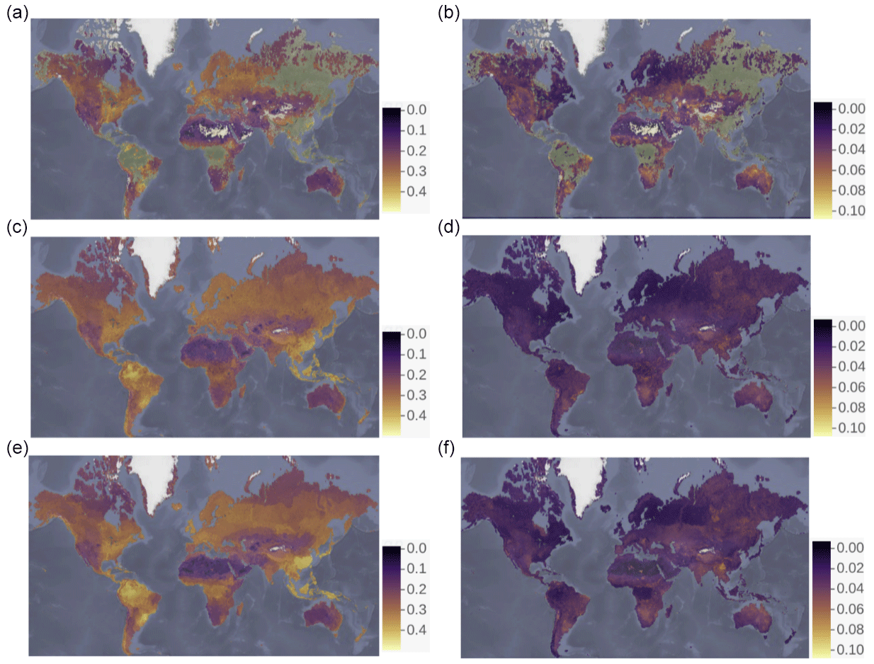
Figure 4Soil moisture mean (a) and variance (b) of the ESA-CCI soil moisture product v4.5 between 1991 and 2018. Prediction of soil moisture (c) and prediction variance (5000×5, d) based on topographic terrain parameters. Prediction of soil moisture (e) and prediction variance (f) based on bioclimatic and soil type classes. Units: m3 m−3.
We provide an example of the sensitivity of our models across tropical areas with low availability of data for training the models as described in Sect. 2.3. For tropical areas of the world with limited information in the ESA-CCI datasets, the cross-validated results of the model predictions showed r values around 0.62 and RMSE values around 0.03 m3 m−3 using terrain parameters and soil type classes (Fig. A3). We find that the model predictions based only on the limited ESA-CCI soil moisture information available across tropical areas (Fig. A3) show a similar prediction variance to the model predictions for the entire world, with values from < 0.001 to < 0.12 m3 m−3 (Fig. A3). These result support the effectiveness of our approach across areas with lower availability of information to train the k-KNN algorithm.
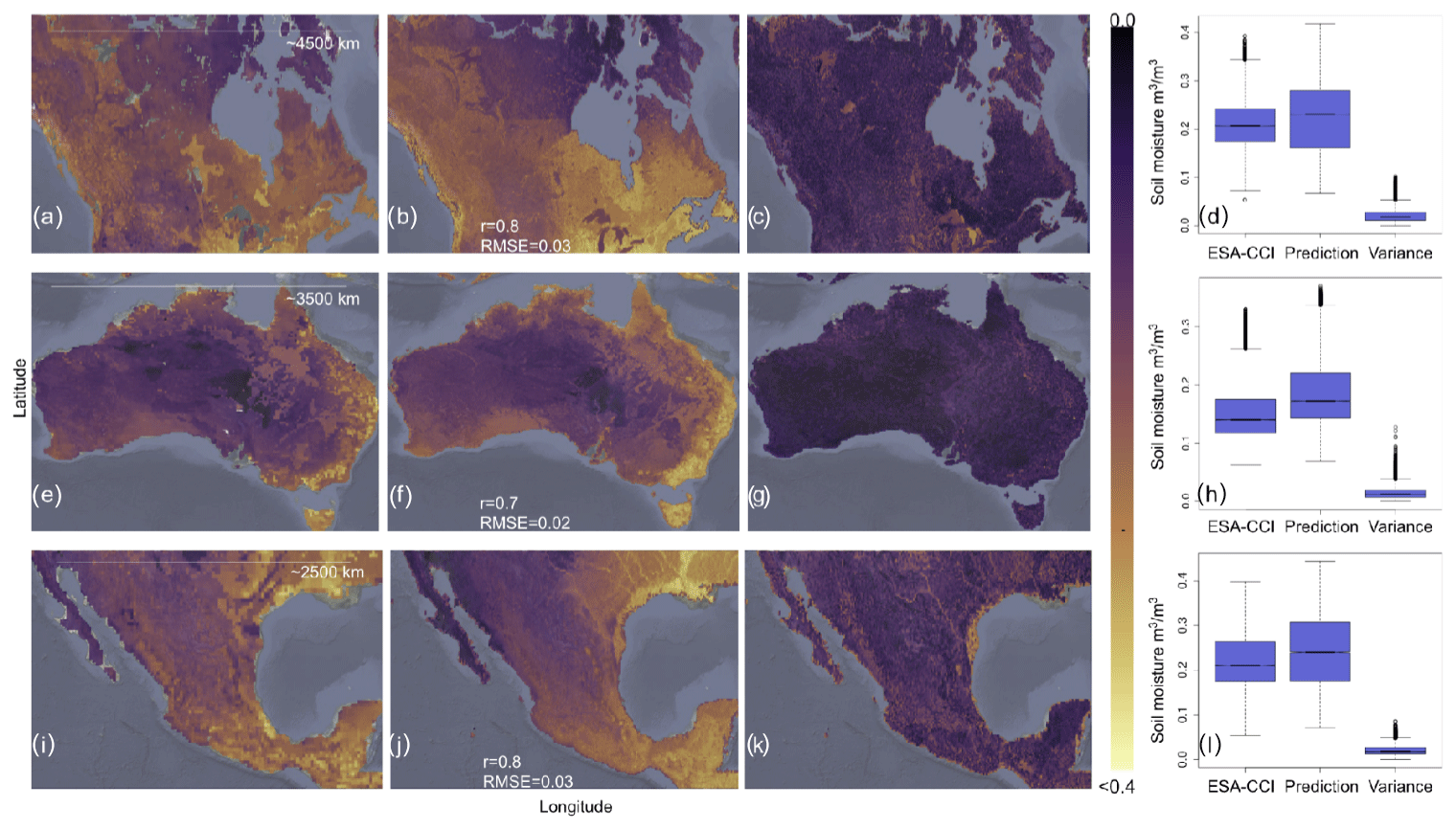
Figure 5Examples of downscaled annual mean soil moisture across specific countries. Prediction of soil moisture, prediction variance, and training data from the ESA-CCI across Canada (CAN; a–c), and their respective boxplots (showing their statistical distribution) for the year 2018 (d). Prediction of soil moisture, prediction variance, and training data from the ESA-CCI across Australia (AUS; e–g), and their respective boxplots for the year 2018 (h). Prediction of soil moisture, prediction variance, and training data from the ESA-CCI across Mexico (MEX; i–k), and their respective boxplots for the year 2018 (l).
We additionally assess the sensitivity of the model predictions across areas of the world with heterogeneous environmental and climate gradients (i.e., geographical extent of countries such as Mexico, Canada, and Australia), generated as described in Sect. 2.3. The ESA-CCI has relatively better spatial coverage across these countries (Fig. 5) compared with tropical areas (Fig. A3) but still has a lower amount of training data compared with models generated for the entire world. Comparing our soil moisture predictions across 15 km grids with the original ESA-CCI soil moisture dataset at 27 km grids (Fig. 8) for these areas, we observe that our soil moisture predictions have consistently higher maximum values (> 0.04 m3 m−3) than the original ESA-CCI soil moisture dataset (< 0.4 m3 m−3) (Fig. 5). We observe consistent modeling accuracy across these countries and across the entire world (in all cases r values > 0.6 and RMSE values around 0.04 m3 m−3).
The last two sets of results for tropical areas with low availability of data and areas of the world with heterogeneous environmental and climate gradients support the effectiveness of our approach across areas exhibiting unfeasible data collection and heterogeneous data characteristics, respectively. The flexibility of our prediction models to generate consistent results on a country-specific basis could be supported by the use of country-specific information (e.g., topographic, bioclimatic, and soil information) to predict soil moisture with higher spatial resolution (< 15 km grids) in future research.
3.3 Relevance of the different prediction factors
Across the entire world, we assess the relevance of the different prediction factors defined in Sect. 2.1 (i.e., prediction factors from terrain parameters, bioclimatic features, and soil type classes) by rebuilding the prediction models using the k-KNN algorithm and removing one prediction factor at a time. By systematically removing one prediction factor at a time and using repeated 10-fold cross-validation (n= 10), we can measure the prediction factor impact on the accuracy of each model generated for each year using the k-KNN algorithm (Fig. 6). To this end, we compare the cross-validation results (r and RMSE values) of each new model against a reference model that we build by using all prediction factors. Each soil moisture prediction using all prediction factors for each year is accompanied by a reference accuracy report containing the cross-validation results (see Sect. 5). We sort the relevance of prediction factors based on the impact of their absence on the cross-validation results (r and RMSE values), compared with the reference models (using all prediction factors) across each year. Specifically, for each year (1991–2018) and for each factor that is removed at the time (42 factors), we repeat the cross-validation 10 times as explained in Sect. 2.2 and compute the mean accuracy. For each factor, we count the number of times when the absence of that factor causes a higher r and a lower RMSE compared with the mean accuracy of the reference model generated for each of the 28 years. Across the years we count the number of positive and negative impacts and show the proportion of times (or impact rate) when the absence of each prediction factor results in a higher accuracy (i.e., higher r and lower RMSE) versus the proportion of times when the absence results in a lower accuracy (i.e., lower r and higher RMSE) (Fig. 6).
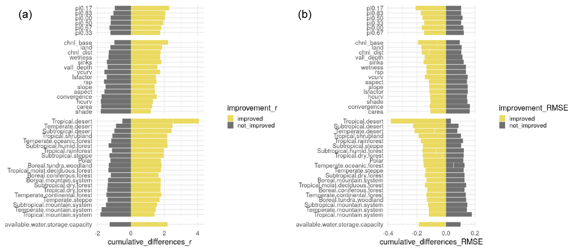
Figure 6Impact of each factor on (a) r and (b) RMSE values across years (1991–2018). The factors with code pi0.00, pi0.17, pi0.33, pi0.50, pi0.67, and pi0.83 are the spatial coordinates rotated at multiple angles shown in Fig. A2. The rest of the factors are the digital terrain parameters used to predict the ESA-CCI annual means as they are shown in Fig. 3 and described by Guevara and Vargas (2019): aspect: terrain aspect; carea: specific catchment area; chnl base: channel network base level; chnl dist: distance to channel network; convergence: flow convergence index; hcurv: horizontal curvature; land: digital elevation model; lsfactor: length–slope factor; rsp: relative slope position; shade: analytical hillshade; sinks: smoothed elevation; slope: terrain slope; vall depth: valley depth index; vcurv: vertical curvature; and wetness: topographic wetness index. The bioclimatic features in (a) tropical, (b) subtropical, (c) temperate, or (e) boreal environments are represented by binomial variables (0–1). These variables are extracted by the Food and Agriculture Organization Global Agro-Ecological Zones project. The available water storage capacity variable is represented by continuous classes available thanks to the Regridded Harmonized World Soil Database.
We sort the relevance of prediction factors based on the impact of their absence on the cross-validation results (r and RMSE values), compared with the reference models (using all prediction factors) across each year: for r (Fig. 6a) a negative impact rate of a factor means that the model tends to improve in accuracy (in terms of higher r) when including that factor, and vice versa a positive impact means that the correlation increased when the factor is removed. In contrast, for RMSE (Fig. 6b) a positive impact means that the model tends to improve accuracy (in terms of lower RMSE) when including that factor, and vice versa a negative impact means that the error decreased when the factor is removed.
We observe that spatial coordinates in rotated angles ranging between 17 and 83∘ (Fig. A2) are coordinates with a positive impact on r and RMSE results across years (Fig. 6). Considering each year in isolation, we observe that values for r and RMSE are consistent across individual years. In Fig. 7 we present the values for r and RMSE for 2018 as a representative case. In 2018, we observe that spatial coordinates rotated in an oblique angle between 33 and 50∘ (variables pi0.33 and pi0.50, Fig. A2) have a high impact on r or RMSE values (Fig. 7a).
Across all years, we find bioclimatic features have a higher impact on r or RMSE values, followed by terrain parameters and soil classes (Fig. 6), which supports further findings in our validation against in situ soil moisture data contained in the augmented ISMN (in Sect. 3.4). We find that the use of spatial coordinates has a similar impact on r and RMSE values compared with terrain parameters or soil type classes (Fig. 6). We observe a slightly higher (but statistically similar) impact of bioclimatic features in cross-validation results compared with terrain parameters (Fig. 6). Bioclimatic features indicating presence or absence (0 or 1 binomial variable, respectively) of tropical, subtropical, or temperate desert (biological and climatological) conditions are variables with a high impact on the cross-validation of prediction models. The distance between the base of drainage network channels and the closest highest point in the ground (before elevation decreases again) (code in Fig. 6: chnl_base) or the distance of each pixel to the closest drainage network channel (code in Fig. 6: chnl_dist) are elevation-derived (code in Fig. 6: land) terrain parameters with a high impact on r and RMSE across all years. We observe for our example with the year 2018 that terrain parameters such as chnl_base and chnl_dist have a higher impact on r and RMSE values consistently with our analysis across all years (1991–2018). Bioclimatic features indicating the presence or absence (0 or 1 binomial variable, respectively) of temperate steppe climate conditions or the presence or absence of tropical shrubland climate conditions become top prediction factors for soil moisture in this specific year (2018, Fig. 7). The impact of terrain parameters has a different impact for predicting soil moisture variability depending on the average amount of water reaching the soil (via precipitation and runoff or overland flow) for each year, which is a process highly dependent on bioclimatic conditions. Thus, we can expect to observe variations in the impact of parameters to predict soil moisture across specific years (e.g., in extremely dry versus extremely wet years). We provide a variable importance plot for each year associated with each soil moisture prediction (see Sect. 5).

Figure 7Impact of each factor on the (a) r and (b) RMSE values for the year 2018. The factors named pi0.00, pi0.17, pi0.33, pi0.50, pi0.67, and pi0.83 are the spatial coordinates at multiple angles shown in Fig. A2. The digital terrain parameters are shown in Fig. 3 and described by Guevara and Vargas (2019): aspect: terrain aspect; carea: specific catchment area; chnl base: channel network base level; chnl dist: distance to channel network; convergence: flow convergence index; hcurv: horizontal curvature; land: digital elevation model; lsfactor: length–slope factor; rsp: relative slope position; shade: analytical hillshade; sinks: smoothed elevation; slope: terrain slope; vall depth: valley depth index; vcurv: vertical curvature; and wetness: topographic wetness index. The bioclimatic features divided into (a) tropical, (b) subtropical, (c) temperate, or (d) boreal environments are represented by binomial variables (0–1). These variables are extracted by the Food and Agriculture Organization Global Agro-Ecological Zones project. The available water storage capacity variable is represented by continuous classes available thanks to the Regridded Harmonized World Soil Database.
3.4 Soil moisture trained for region for which augmented ISMN datasets exist
To compare soil moisture values between our predictions and the augmented ISMN, we follow two main steps. First, we assess the r and RMSE values between the ESA-CCI dataset and our soil moisture predictions against in situ soil moisture using the augmented ISMN. Second, we report changes of soil moisture over time using the augmented ISMN, the ESA-CCI, and our soil moisture predictions.
Comparing the correlation between in situ and gridded soil moisture datasets, we observe that the correlation of the ESA-CCI (v4.5) with the augmented ISMN across the world is lower compared to the correlation between soil moisture predictions based on digital terrain analysis with the ISMN or soil moisture predictions adding bioclimatic and soil type classes (Fig. 8).
When all available data across all soil depths per site in the augmented ISMN are considered (n= 2185 stations), the r values show a mean of 0.50 between the ISMN and the ESA-CCI, the predictions based on digital terrain parameters show an r value of 0.56, and the predictions including bioclimatic and soil type classes show an r value of 0.65. Similar levels of RMSE against the ISMN are found with the models using bioclimatic and soil type classes (∼ 0.05 m3 m−3) or models using only terrain parameters (∼ 0.05 m3 m−3). When comparing the ISMN and the ESA-CCI, we observe a mean RMSE of 0.09 m3 m−3. Confirming these results, by restricting our validation strategy only to the sites with available information for the first 0–5 cm of soil depth (n= 987 stations), we observe correlation values varying from 0.46 for the ESA-CCI (RMSE 0.05 m3 m−3) to 0.86 using topographic prediction factors (RMSE 0.03 m3 m−3) and 0.74 using bioclimatic and soil type classes (RMSE 0.05 m3 m−3) as is shown in Fig. 8a–f. The target diagram presented in Appendix A, Fig. A4, is also useful for visualizing the improvement of our approach over the original ESA-CCI soil moisture dataset.
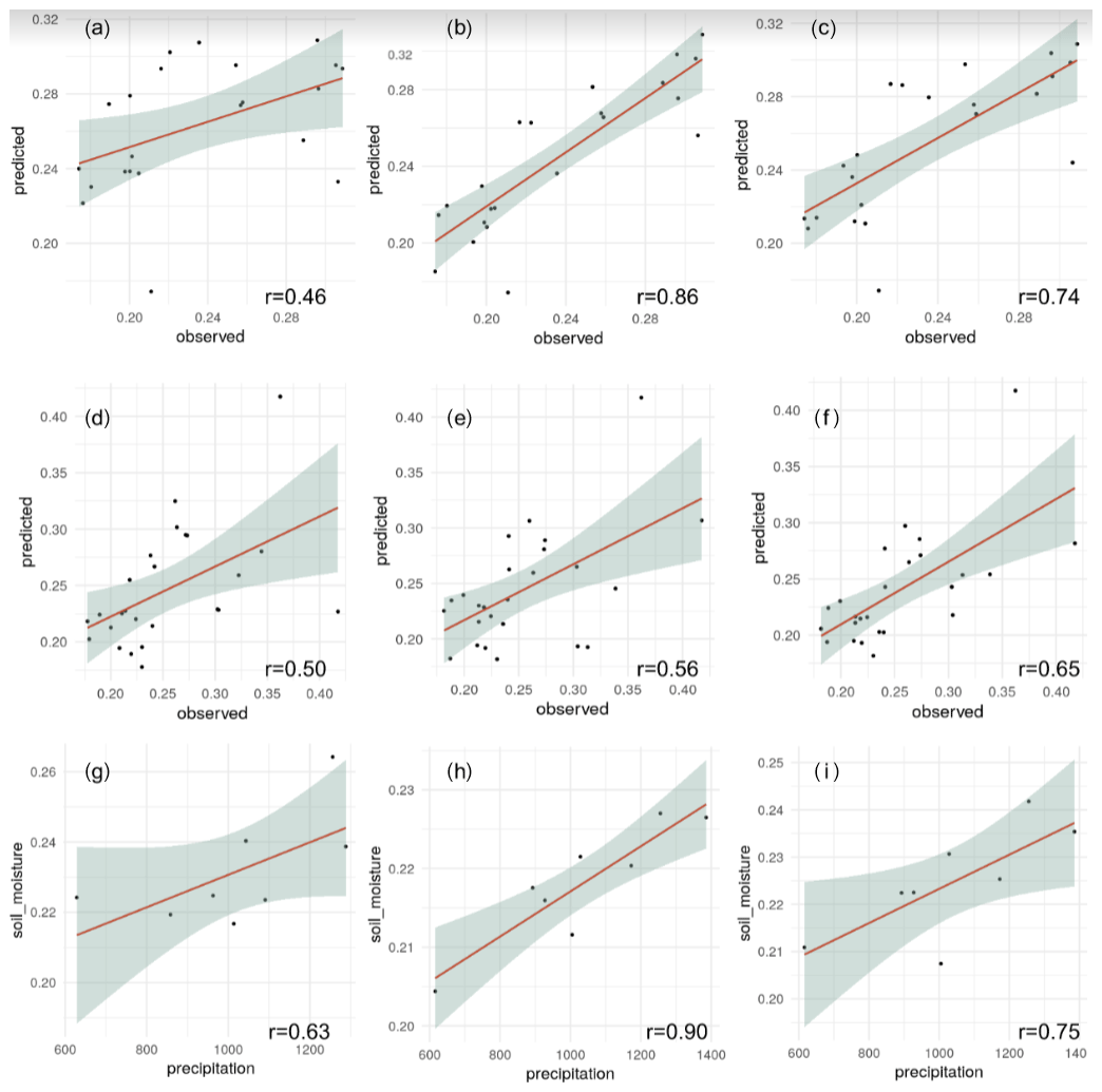
Figure 8Model evaluation plots (points vs. grids) of mean annual values of soil moisture across the world. ISMN against the ESA-CCI (a), ISMN against the predictions based on terrain analysis (b), and ISMN against the predictions based on the model using bioclimatic and soil type classes (c) for the sites with available information between 0–5 cm (n= 987 stations). We also show the correlation between the ESA-CCI (d) and our predictions based on terrain parameters (e) or bioclimatic and soil type classes (f) using all available data in the ISMN across all soil depths (n= 2185 stations). The panels below show the correlation between soil moisture grids and in situ mean annual precipitation records and in situ precipitation against the ESA-CCI (g), in situ precipitation against predictions based on terrain analysis (h), and in situ precipitation against predictions based on the model using bioclimatic and soil type classes (i).
Across all analyzed years, our global soil moisture predictions represent an improvement as they reduce bias when compared with the ISMN data and in situ precipitation records. The variance around the prediction error (e.g., the unbiased RMSE) estimated against the augmented ISMN was also lower in our predictions compared with the ESA-CCI soil moisture dataset (Appendix A, Fig. A4).
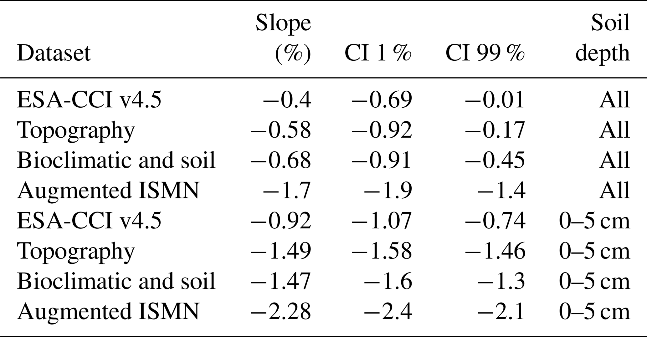
We confirm the effectiveness of the k-KNN algorithm for modeling and predicting soil moisture considering changes in soil moisture levels over time (soil moisture trends, Table 1). There is a consistent soil moisture decline over time across all soil moisture datasets (i.e., the augmented ISMN and the ESA-CCI datasets; the soil moisture predictions based on digital terrain analysis; and the predictions using digital terrain analysis, bioclimatic, and soil type classes; Table 1) at the specific locations of the augmented ISMN dataset (Fig. 1). Supporting the effectiveness of the model predictions, all datasets (observed and modeled soil moisture) show negative soil moisture trends at locations where all datasets exist (Table 1).
Table 1The slope and slope uncertainties of soil moisture trends at the locations where all datasets exist. We show the dataset, the slope (%), and the lower and upper confidence interval (CI). We report negative trends considering all available data across all soil depths (n= 2185 stations) and across sites with information available only between 0–5 cm of soil depth (n= 987 stations).
3.5 Soil moisture trained for region with limited ISMN dataset availability
To compare soil moisture values across the entire world, we follow two main steps. First, we assess soil moisture trends across areas with no available data in the augmented ISMN using in situ precipitation data (Fig. 1, blue). Second, we assess changes over time across the areas with available data in the ESA-CCI dataset. Third, we assess changes of soil moisture across the world using our soil moisture predictions.
Comparing the correlation of the ESA-CCI and our soil moisture predictions, we observe that our predictions are better correlated with in situ precipitation records across areas with no available data in the augmented ISMN (Fig. 8g–i). Aggregated in yearly means, we observe a correlation between precipitation data and the ESA-CCI of 0.63, a correlation of 0.86 between precipitation data and the soil moisture predictions based on terrain parameters, and a correlation of 0.75 between precipitation data and the soil moisture predictions based on bioclimatic and soil type classes. These results support the model predictions across areas with low availability of in situ soil moisture validation data.
When analyzing changes of soil moisture over time using the ESA-CCI dataset across the entire world (when available), we observe significant soil moisture increase (positive trend) over time across ∼ 70 000 km2 of the global land area (> 500 million km2) using a probability threshold of 0.05 with available data from 1991 and 2018. We also observe a significant decline (negative trend) of soil moisture across 43 740 km2 of global land area (Fig. 9a–b). In contrast, across the entire world, soil moisture based on terrain parameters shows > 60 million km2 of global land area with negative trends and 274 147 km2 with positive trends (Fig. 9c–d).
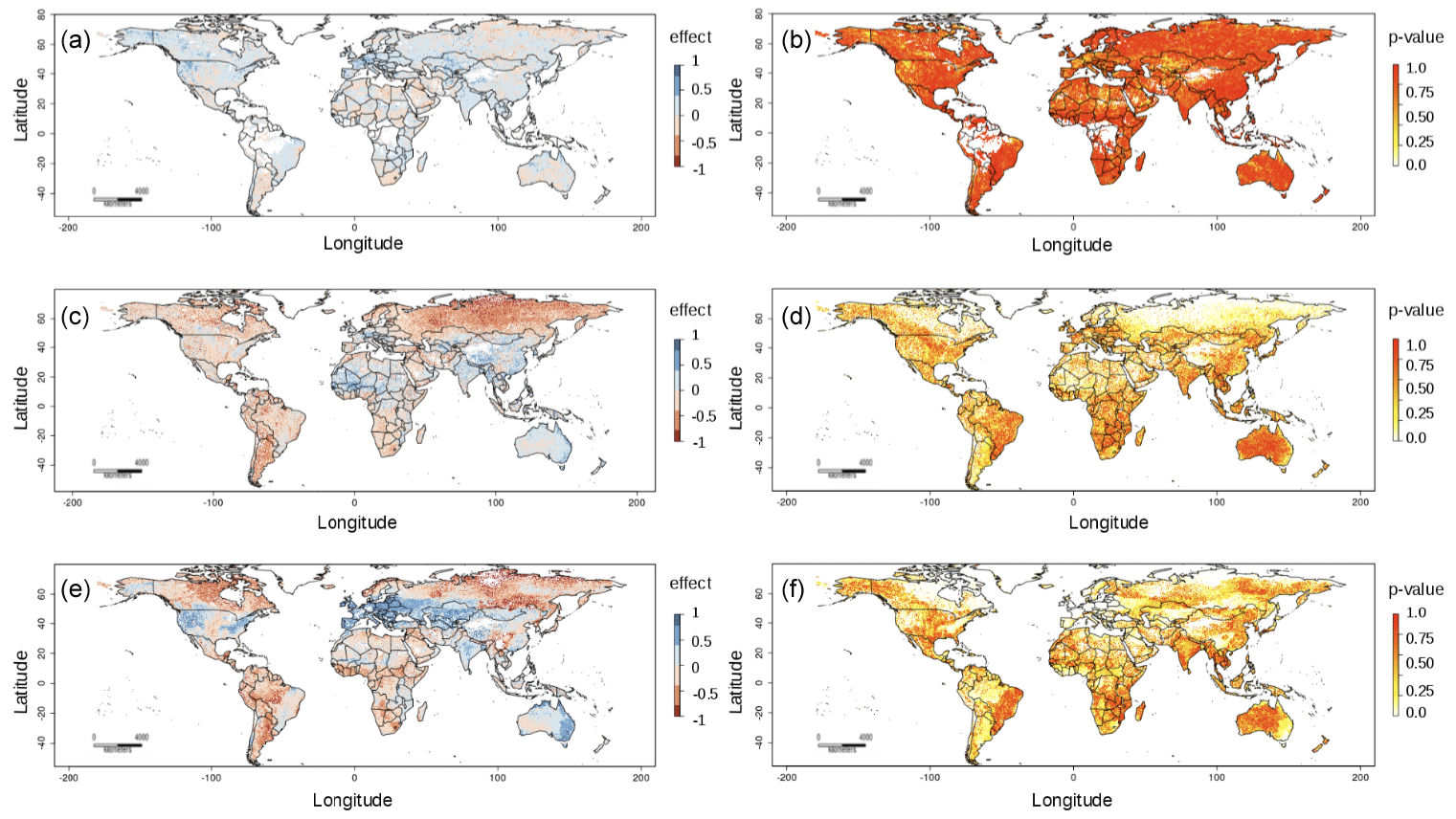
Figure 9Trends of the ESA-CCI annual means (a) and their respective probability values (b). Trends of the soil moisture predictions based on digital terrain parameters (c) and their respective probability values (d). Trends of soil moisture predictions using terrain parameters, bioclimatic features, and soil type features (e) and their respective probability values (f).
The soil moisture predictions based on terrain parameters and bioclimatic and soil type features show significant negative trends (probability threshold < 0.05) across 216 246 km2 and positive trends across 85 991 km2 (Fig. 9e–f) of global land area. Discrepancies between the ESA-CCI and our downscaled datasets are in part because our results predict soil moisture decline across areas with large gaps in the ESA-CCI, such as tropical areas. For example, with our soil moisture predictions we observe emergent negative trends of soil moisture across tropical rain forests of the Amazon Basin and the Congo region.
We present a regression approach coupling k-KNN and digital terrain analysis for improving the spatial resolution (i.e., improving spatial granularity) of ESA-CCI satellite soil moisture estimates by nearly 50 % and providing a gap-free global annual mean soil moisture dataset (with associated prediction variances) for the years 1991–2018. In this section we interpret and describe the significance of the new soil moisture datasets (based on terrain continuous parameters, soil and climate classes) in light of what was already known thanks to state-of-the-art satellite soil moisture (e.g., from the ESA-CCI) about the research problem of accuracy, coarse granularity, and spatial gaps of soil moisture information at the global scale (i.e., incomplete global coverage).
We outline the key findings and insights organized in terms of their impact. First, we highlight the main improvements of the new soil moisture dataset over the ESA-CCI soil moisture product. Second, we discuss the role of terrain parameters in the accuracy of the newly generated dataset. Third, we discuss emergent soil moisture trends before and after taking our new datasets into consideration. Fourth, we discuss potential sources of variance and discrepancy between soil moisture datasets (e.g., augmented ISMN, ESA-CCI, our predictions). Fifth, we provide information about the main limitations of the new dataset. Sixth, we discuss opportunities for future work.
We highlight the main improvements of the new soil moisture dataset over the ESA-CCI soil moisture product. Our predictions of soil moisture against the ESA-CCI soil moisture product show an improvement in the reduction of bias when compared with in situ soil moisture datasets (i.e., with the ISMN; Fig. 8 and Appendix A, Fig. A4). Improving the accuracy and spatial resolution of satellite-derived soil moisture is an ongoing challenge that requires different approaches. For example, recent soil moisture remote sensing datasets (Entekhabi et al., 2010; Piles et al., 2019) are able to provide information across areas with spatial gaps in the ESA-CCI; however, only recent years have full soil moisture coverage (e.g., 2010 to date). Our results represent a long-term (1991–2018) and gap-free soil moisture dataset and represent a response to the need of alternative global-to-regional soil moisture datasets (An et al., 2016; Colliander et al., 2017b; Dorigo et al., 2011b; Minet et al., 2012; Mohanty et al., 2017; Yee et al., 2016). This dataset has implications for further analyses on soil moisture patterns (Berg and Sheffield, 2018), global hydrological models (Zhuo and Han, 2016), climate change predictions (Samaniego et al., 2018), carbon cycling models (Green et al., 2019), and food security assessments (Mishra et al., 2019).
We now discuss the role of terrain parameters in the prediction accuracy of the newly generated dataset. We have demonstrated the role of topographic terrain parameters as a parsimonious and effective approach for downscaling satellite-derived soil moisture in terms of r (Fig. 6) or RMSE (Fig. 7). Terrain parameters are available nowadays with unprecedented levels of spatial resolution (i.e., meters), and our approach is potentially applicable to specific areas or countries (Fig. 5) and higher spatial resolution (Guevara and Vargas, 2019). Our results support the value of terrain parameters as the basis for downscaling soil moisture satellite estimates in future research across specific areas or periods of time. The exclusive use of terrain parameters in our algorithm implementation (Sect. 2.2) can help to reduce model complexity and computational expenses of more complex models using an extensive set of prediction factors for representing soil variability (e.g., Hengl et al., 2017). A soil moisture dataset independent of bioclimatic and soil information is useful for preventing potential spurious correlations in further studies. This is specifically important for studies dealing with the problem of interpreting machine learning frameworks or better understanding the use of data by the algorithms to generate accurate model predictions (Padarian et al., 2020; Ribeiro et al., 2016). On the other hand, predicting soil moisture considering tacit knowledge (i.e., expert opinion) on variable selection (e.g., manually combining multiple combinations of prediction factors and discussing with experts the resulting maps) may also be useful to complement the assessment of model accuracy and to develop interpretable and parsimonious models for global soil moisture mapping. Our results suggest that a parsimonious model based on topography shows comparable accuracy to a more complex model including bioclimatic and soil type classes (Figs. 6–8, Appendix A, Fig. A4) and similar negative trends (Table 1). Although ML approaches generally benefit from using multiple prediction factors to represent patterns, we advocate for simpler models. The parsimonious approach (based on topography) does not necessarily reduce prediction capacity when compared with a more complex model adding bioclimatic and soil type classes, and both datasets show a similar trend of soil moisture levels over time.
Our trend detection analysis reveals changes of soil moisture over time at the global scale, across areas with limited information in the ESA-CCI dataset or areas where the augmented ISMN does not exist. We observe consistent soil moisture decline at the global scale using both the soil moisture predictions based on topography and the predictions based on topography, bioclimatic features, and soil classes. The soil moisture trend of the augmented ISMN dataset was also negative (Table 1). These soil moisture trends have potential implications for the calibration of future projections of the water cycle, for identifying regions of strong land–atmosphere coupling (Lorenz et al., 2015), and for quantifying the contribution of soil moisture for land surface models (Singh et al., 2015). The negative soil moisture trends found in this study (Fig. 9) are consistent with recent soil moisture monitoring efforts (Albergel et al., 2013; Gu et al., 2019a). It has been shown that soil moisture decline can be intensified by land warming (Samaniego et al., 2018), land use change (Chen et al., 2016; Garg et al., 2019), agricultural practices (Bradford et al., 2017), or transformations to vegetation cover that directly affect primary productivity, evapotranspiration rates, and drought (Stocker et al, 2019; Martens et al., 2018). Furthermore, contiguous information on soil moisture trends is increasingly needed to quantify the consequences of soil moisture decline in ecosystem processes such as soil respiration (Bond-Lamberty et al., 2018). Our results complement the ESA-CCI soil moisture dataset as they identify soil moisture decline across the Congo region or the Amazon Basin (Fig. 9). These results are consistent with previous studies that have identified soil moisture decline across the Congo region associated with reduction of precipitation rates (Nogherotto et al., 2013) and across the Amazon Basin, where climate signals in plant productivity could be due to changes in soil moisture conditions (Wagner et al., 2017). Further studies are needed to fully interpret the influence of surface or deeper soil moisture on ecological processes (Morton et al., 2014), but we argue that surface soil moisture trends are critical to identify potentially vulnerable regions across the world. Our examples of surface soil moisture predictions across tropical areas (using the available ESA-CCI information) or across specific countries with heterogeneous environmental gradients (e.g., Fig. 5) are consistent in terms of prediction accuracy, suggesting that our approach is applicable to any country or region in the world, including areas with limited information with which to feed prediction algorithms.
Limitations of our approach include (a) the propagation of measurement errors of the ESA-CCI dataset used to train the k-KNN algorithm, (b) the propagation of measurement errors (and quality) of the digital elevation dataset used for calculating terrain parameters, and (c) the prediction errors of the k-KNN algorithm (e.g., random errors, systematic errors, spatially autocorrelated errors). It is known that satellite-derived soil moisture estimates fail to measure extremely dry or extremely wet conditions (McColl et al., 2017; Liu et al., 2019); consequently, this lack of information influences the prediction capacity of our downscaling framework, and there is a need to improve modeling and measurements of these extremes. In addition, the quality of the prediction factors impacts the quality of final prediction outcomes. Thus, the prediction algorithm is not able, in any case, to generate a perfect model. Therefore, it is important to provide prediction variances around soil moisture predictions that are useful for identifying areas with high or low model consistency (Fig. 4). The variance associated with soil moisture predictions provides novel information with which to assess the strength of the relationship between the covariate space (e.g., terrain parameters, bioclimatic and/or soil type features) and predicted soil moisture. Consequently, large prediction variances (Fig. A3) remain across areas less represented in both field measurements (Fig. 1) and across extremely dry or extremely wet conditions affecting the spatial representation of satellite soil moisture datasets (Fig. 4a). Our prediction variances also provide insights for future research efforts where alternative techniques are needed to provide information to better constrain model predictions and to reduce prediction variances.
We discuss potential sources of prediction variance between soil moisture predictions and datasets. Prediction variances are indicators of discrepancy levels between soil moisture datasets (augmented ISMN, ESA-CCI, our predictions). Discrepancy between the augmented ISMN and satellite-derived soil moisture or our downscaled datasets can be associated with differences in the spatial representativeness of point measurements and grid surfaces (Gruber et al., 2020). This scale mismatch has been previously identified when testing different soil moisture patterns (Nicolai-Shaw et al., 2015) as field soil moisture records are usually representative of < 1 m3 of soil, while satellite and modeling estimates vary from several meters to multiple kilometers. Soil moisture measurements (from satellites and in situ measurements) across both water-limited environments and tropical areas are extremely limited (Liu et al., 2019), a condition that increases prediction variances (and consequently also increases model uncertainty). Thus, alternative modeling and evaluation frameworks and model evaluation statistics are required to provide more information to better interpret the spatial variability and dynamics of soil moisture global estimates (Gruber et al., 2020). To this end, we used in situ annual precipitation as a proxy to evaluate soil moisture estimates and found that our predicted soil moisture was better correlated than the original ESA-CCI dataset. This higher correlation may be useful for further analyses and evaluations, including soil moisture and precipitation feedbacks (McColl et al., 2017), as precipitation decline has been associated with soil moisture decline in previous studies (Nogherotto et al., 2013).
Future work should include predicting global soil moisture patterns across finer pixel sizes (e.g., 1 km or < 1 km) and higher temporal resolutions (e.g., monthly or daily), as has been done at regional to continental scales (Naz et al., 2020; Llamas et al., 2020; Guevara and Vargas, 2019). The current version of the downscaled soil moisture predictions is provided on an annual basis because it is a temporal resolution useful for multiple ecological and hydrological studies related to large-scale ecological processes and climate change (Green et al., 2019). We recognize that there is an increasing need for soil moisture datasets with higher temporal resolutions to analyze the seasonal and short-term memory soil moisture effects after precipitation events (McColl et al., 2017). A spatial resolution of 15 km is still a coarse pixel size for detailed analysis of hydro-ecological patterns (e.g., at the hillslope scale), but the main focus of this study was to test the potential of digital terrain analysis for increasing the spatial resolution of the original ESA-CCI soil moisture dataset. Our decision for selecting a 15 km pixel size was driven by the reproducibility of our approach by multiple groups without the need for high-performance computing (HPC) infrastructure. HPC is increasingly required for modeling soil moisture patterns with unprecedented levels of spatial resolution across continental scales (e.g., 3 km grids, RMSE of 0.04 to 0.06 m3 m−3; Naz et al., 2020) that show comparable accuracy to our 15 km grids (Fig. 8a–c). Additionally, the increase of nearly 50 % in spatial resolution suggests a larger range of predicted soil moisture values compared with the ESA-CCI, possibly associated with scale-dependent patterns of soil moisture (Fig. 5), which can be analyzed in future work.
In conclusion, to downscale (i.e., increase spatial resolution) coarse satellite soil moisture grids, we used k-KNN to combine satellite soil moisture data with terrain parameters (as surrogates of topographic variability) and bioclimatic and soil type classes. The validation of our soil moisture model predictions against multiple field data sources (Fig. 1) and multiple combinations of prediction factors supports the notion that digital terrain analysis can be used as a parsimonious approach for improving the spatial resolution of the ESA-CCI soil moisture dataset (Appendix A, Fig. A4). We provide a new gap-free and annual soil moisture dataset for 28 years provided across 15 km grids on an annual basis (1991–2018). Our results provide a global soil moisture benchmark to address the increasing need for soil moisture datasets with higher temporal and spatial resolution at the global scale.
We provide a publicly available soil moisture dataset including working codes and information useful for replicating our results. We follow global validation standards for modeled soil moisture estimates (Gruber et al., 2020). We also provide the prediction variance maps derived from bootstrapping the results of each modeled year (as surrogates of prediction uncertainty) and user guidance for interpreting and reproducing our results. The sources of information required to develop this study are as follows:
-
The soil moisture training dataset used in this study is available thanks to the ESA-CCI (https://www.esa-soilmoisture-cci.org/, last access: 20 April 2021, Dorigo et al., 2017; Liu et al., 2011)
-
The soil moisture validation dataset used in this study is available thanks to the ISMN (https://ismn.geo.tuwien.ac.at/en/, last access: 20 April 2021, Dorigo et al., 2011a)
-
The downscaled soil moisture predictions generated in this study are available in Guevara et al. (2020, https://doi.org/10.4211/hs.9f981ae4e68b4f529cdd7a5c9013e27e)
-
The soil moisture predictions are provided in rasters (n= 28 per folder, 1991–2018) that can be imported into any GIS, and they contain an accuracy report from the cross-validation for each model/year in a *.csv file.
-
We include a raster stack with 28 layers containing the prediction variances for each model year (1991–2018) derived from bootstrapping the k-KNN models.
-
The prediction factors for soil moisture across 15 km grids are also available in an R spatial pixel data frame, containing values for each pixel of
- a.
terrain parameters calculated in SAGA-GIS http://www.saga-gis.org/ (last access: 20 April 2021),
- b.
bioclimatic classes from http://www.fao.org/nr/gaez/en/ (last access: 20 April 2021) transformed into a binary presence or absence (1 or 0, respectively) code and
- c.
the continuous classes (1: 150 mm water per m of the soil unit; 2: 125 mm; 3: 100 mm; 4: 75 mm; 5: 50 mm; 6: 15 mm; and 7: 0 mm) from the Regridded Harmonized World Soil Database v1.2 (available here: https://daac.ornl.gov/SOILS/guides/HWSD.html, last access: 20 April 2021, Wieder et al., 2014).
- a.
-
In the same data repository, we provide the ISMN (downloaded in August of 2019) annual dataset that we used for validating (Fig. 1, green) our soil moisture predictions in a native R spatial object.
-
Figure A5 of this dataset includes a summary of soil moisture values per contributing network in the ISMN. All contributing networks can be found at https://ismn.geo.tuwien.ac.at/en/networks/ (last access: 20 April 2021) thanks to the ISMN initiative.
-
-
-
The precipitation dataset used as alternative validation data (Fig. 1, blue) is available here: https://daac.ornl.gov/SOILS/guides/SRDB_V4.html (last access: 20 April 2021, Bond-Lamberty,and Thomson, 2018).
-
Additional soil moisture data from local studies (Fig. 1, red) across tropical areas are available here: https://iopscience.iop.org/article/10.1088/1748-9326/7/3/035704 (last access: 20 April 2021, Vargas, 2012) and https://daac.ornl.gov/LBA/guides/CD32_Brazil_ Flux_Network.html (last access: 20 April 2021, Saleska et al., 2013).
-
The R code used (a) to develop our soil moisture modeling and validation approach and (b) to generate the base figures in this paper is available here: https://github.com/vargaslab/Global_Soil_Moisture (last access: 20 April 2021).
As this paper is the result of an active line of research, we will continue updating our soil moisture predictions and our results as new input data (ESA-CCI future versions) become available. The current version covers the period of time between 1991 and 2018, and it is based on the ESA-CCI version 4.5.
A1 Data gaps per year during research period

Figure A1Number of data gaps or not available values (NAs) × 100 in the ESA-CCI v4.5 across years during the analyzed period.
A2 Maps of spatial coordinates
We present the maps of the spatial coordinates used in our prediction approach. We developed these maps following the recently proposed method by Møller et al. (2020). In this method, latitude and longitude across the area of interest (e.g., the entire world) are rotated along several (e.g., n= 6) axes tilted at oblique angles (Fig. A1) and used as prediction factors for soil attributes (e.g., soil moisture).
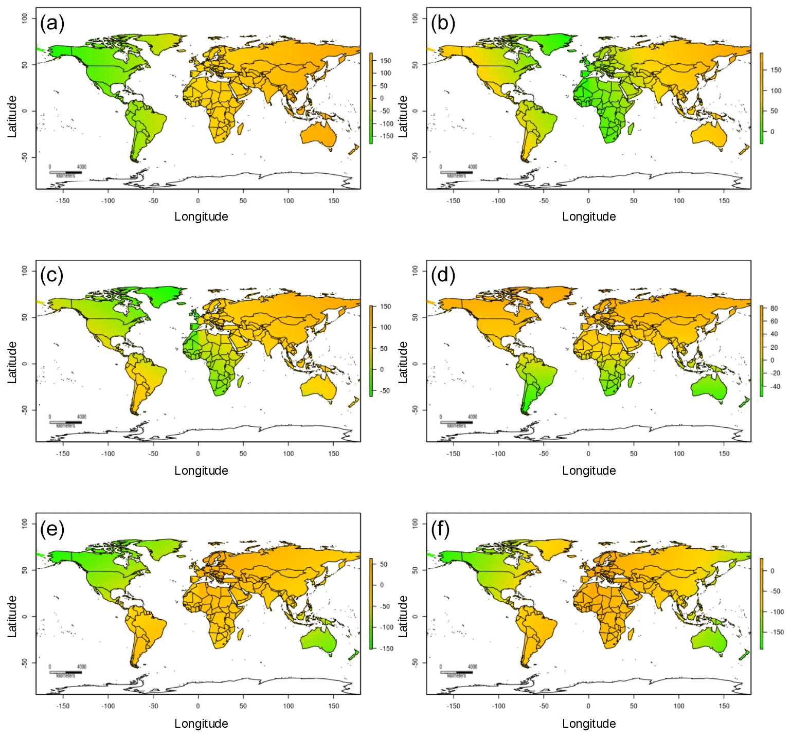
Figure A2The variables pi0.00 (a), pi0.17 (b), pi0.33 (c), pi0.50 (d), pi0.67 (e), and pi0.83 (f) are spatial coordinates of the global 15 km grids tilted at multiple angles (n= 6) used as ancillary information in order to explicitly account for the spatial structure of available soil moisture values in the geographical space.
A3 Data availability in the ESA-CCI soil moisture
We present the availability of data in the ESA-CCI soil moisture data for a given year (e.g., 2018) across tropical areas of the world (Fig. A2a). Using this limited information only (the ESA-CCI data across the tropics), we improve the spatial representativeness of satellite soil moisture data following our prediction approach (Fig. A2b). Our approach considers the model prediction variance after n model realizations (Fig. A2c).
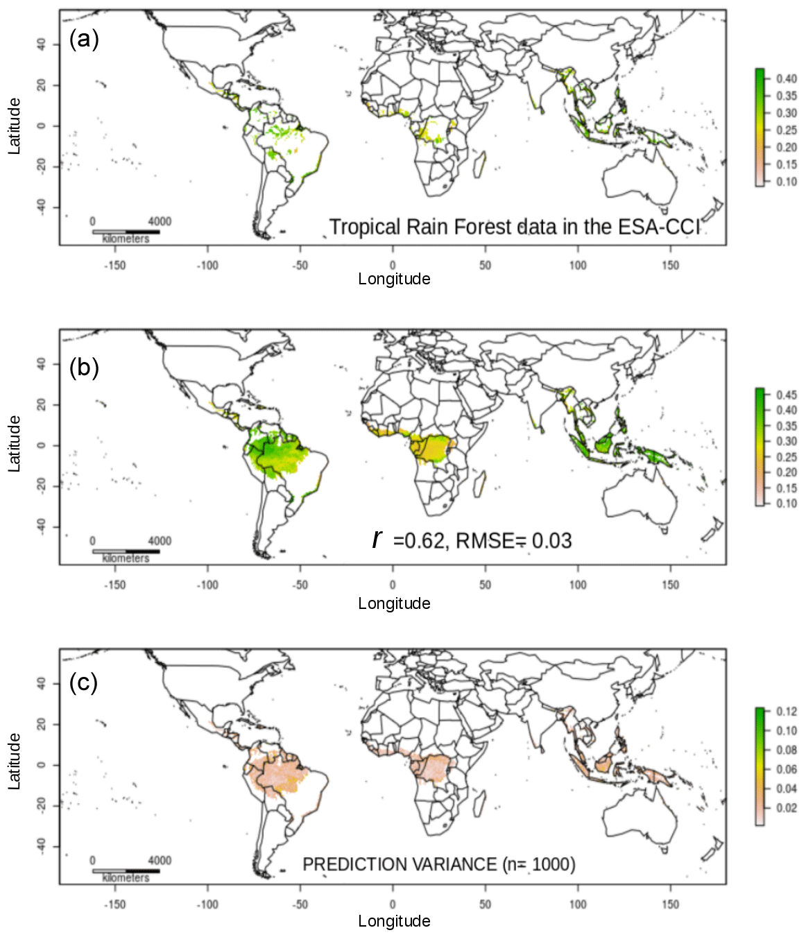
Figure A3Soil moisture across tropical rain forests of the world based on the data available in the ESA-CCI soil moisture product (4.5) for the year 2018 (a). We show the soil moisture prediction (b) and the soil moisture prediction variance using only the data available for tropical rain forests (c). Note that the correlation between observed and predicted decreased to 0.62, most likely due to the limited information for modeling these ecosystems; however the root mean squared error is comparable with a model using all global data (e.g., < 0.04).
A4 Summary of soil moisture validation
We present a summary of our validation of soil moisture predictions in the form of a target diagram (Fig. A3). A target diagram is derived from the relation between the unbiased RMSE, MBE (mean bias error), and RMSE. In a Cartesian coordinate system, the x axis represents the unbiased RMSE (variance of the error), and the y axis represents the MBE. Therefore, the distance from any point to the origin is equal to the RMSE. Because the unbiased RMSE is always positive, the left area of the coordinate system is empty with this scheme. With additional information this region may be also used: the unbiased RMSE is multiplied by the sign of the difference between the standard deviations of model and observations. The diagram provides three different measures: whether the model overestimates or underestimates (positive or negative values of the MBE on the y axis, respectively), whether the model standard deviation is larger or smaller than the standard deviation of the measurements (positive or negative values on the x axis, respectively), and the error performance as quantified by the RMSE represented as the distance to the coordinates origin (see Jolliff et al., 2009).
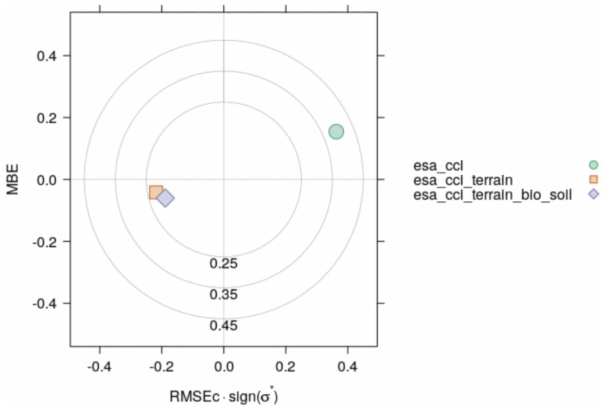
Figure A4Target diagram showing the performance of our soil moisture predictions. The x axis represents the unbiased RMSE (variance units of the error), and the y axis represents the MBE. This figure shows that our soil moisture predictions using terrain parameters (esa_cci_terrain) and the predictions using terrain parameters and bioclimatic and soil type classes (esa_cci_terrain_bio_soil) show lower error levels when compared with field data (from the ISMN) than the ESA-CCI soil moisture product (esa_cci).
A5 Summary of soil moisture values
We present a summary of soil moisture values per contributing network in the ISMN.
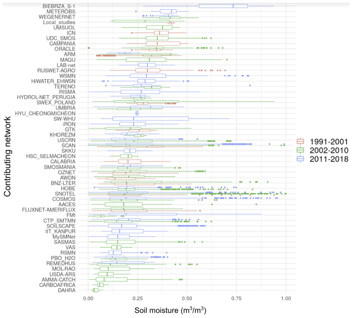
Figure A5A list of contributing networks across the analyzed period of time (organized into three main periods to simplify the figure) and soil moisture values used to compare the ESA-CCI v4.5 and our soil moisture predictions. General information of each network can be found at https://ismn.geo.tuwien.ac.at/en/networks/ (last access: 20 April 2021) thanks to the ISMN initiative.
MG, RV, and MT conceptualized the project. MG performed analysis and wrote the manuscript in collaboration with RV and MT.
The authors declare that they have no conflict of interest.
Mario Guevara acknowledges support from a CONACyT doctoral fellowship (382790). Rodrigo Vargas and Michela Taufer acknowledge support from the National Science Foundation (grant no. 1724843). We thank Anita Z. Schwartz from the University of Delaware for her assistance preparing the global zterrain dataset.
This research has been supported by the National Science Foundation, Directorate for Computer and Information Science and Engineering (grant no. 1724843).
This paper was edited by David Carlson and reviewed by two anonymous referees.
Albergel, C., Dorigo, W., H, R. R., Balsamo, G., de Rosnay, P, MuñozSabater, J., Isaksen, L., de Jeu, R., and Wagner, W.: Skill and Global Trend Analysis of Soil Moisture from Reanalyses and Microwave Remote Sensing, J. Hydrometeorol., 14, 1259–1277, 2013.
Alemohammad, S. H., Kolassa, J., Prigent, C., Aires, F., and Gentine, P.: Global downscaling of remotely sensed soil moisture using neural networks, Hydrol. Earth Syst. Sci., 22, 5341–5356, https://doi.org/10.5194/hess-22-5341-2018, 2018.
Al-Yaari, A., Wigneron, J.-P., Dorigo, W., Colliander, A., Pellarin, T., Hahn, S., Mialon, A., Richaume, P., Fernandez-Moran, R., Fan, L., Kerr, Y. H., and De Lannoy, G.: Assessment and inter-comparison of recently developed/reprocessed microwave satellite soil moisture products using ISMN ground-based measurements, Remote Sens. Environ., 224, 289–303, https://doi.org/10.1016/j.rse.2019.02.008, 2019.
An, R., Zhang, L., Wang, Z., Quaye-Ballard, J. A., You, J., Shen, X., Gao, W., Huang, L., Zhao, Y., and Ke, Z.: Validation of the ESA CCI soil moisture product in China, Int. J. Appl. Earth Observ. Geoinf., 48, 28–36, https://doi.org/10.1016/j.jag.2015.09.009, 2016.
Bauer-Marschallinger, B., Paulik, C., Hochstöger, S., Mistelbauer, T., Modanesi, S., Ciabatta, L., Massari, C., Brocca, L., and Wagner, W.: Soil Moisture from Fusion of Scatterometer and SAR: Closing the Scale Gap with Temporal Filtering, Remote Sens., 2018, 1030, https://doi.org/10.3390/rs10071030, 2018.
Becker, J. J., Sandwell, D. T., Smith, W. H. F., Braud, J., Binder, B., Depner, J., Fabre, D., Factor, J., Ingalls, S., Kim, S.-H., Ladner, R., Marks, K., Nelson, S., Pharaoh, A., Trimmer, R., Rosenberg, J. V., Wallace, G., and Weatherall, P.: Global Bathymetry and Elevation Data at 30 Arc Seconds Resolution: SRTM30_PLUS, Mar. Geod., 32, 355–371, https://doi.org/10.1080/01490410903297766, 2009.
Berg, A. and Sheffield, J.: Climate Change and Drought: the Soil Moisture Perspective, Curr. Clim. Change Rep., 4, 180–191, https://doi.org/10.1007/s40641-018-0095-0, 2018.
Behrens, T., Schmidt, K., MacMillan, R. A., and Viscarra Rossel, R. A.: Multi-scale digital soil mapping with deep learning, Sci. Rep., 8, 1–9, https://doi.org/10.1038/s41598-018-33516-6, 2018.
Bond-Lamberty, B. P. and Thomson, A. M.: A Global Database of Soil Respiration Data, Version 4.0, ORNL DAAC, Oak Ridge, Tennessee, USA, https://doi.org/10.3334/ORNLDAAC/1578, 2018.
Bond-Lamberty, B., Bailey, V. L., Chen, M., Gough, C. M., and Vargas, R.: Globally rising soil heterotrophic respiration over recent decades, Nature 560, 80–83, 2018.
Bradford, J. B., Schlaepfer, D. R., Lauenroth, W. K., Yackulic, C. B., Duniway, M., Hall, S., Jia, G., Jamiyansharav, K., Munson, S. M., Wilson, S. D., and Tietjen, B.: Future soil moisture and temperature extremes imply expanding suitability for rainfed agriculture in temperate drylands, Sci. Rep., 7, 12923, https://doi.org/10.1038/s41598-017-13165-x, 2017.
Chen, X., Su, Y., Liao, J., Shang, J., Dong, T., Wang, C., Liu, W., Zhou, G., and Liu, L.: Detecting significant decreasing trends of land surface soil moisture in eastern China during the past three decades (1979–2010), J. Geophys. Res.-Atmos., 121, 5177–5192, https://doi.org/10.1002/2015jd024676, 2016.
Chung, D., Dorigo, W., De Jeu, R., Kidd, R., and Wagner, W.: ESA Climate Change Initiative Phase II – Soil Moisture, Product Specification Document (PSD), D.1.2.1 Version 4.4; Earth Observation Data Centre for Water Resources Monitoring (EODC) GmbH, Vienna, Austria, p. 49, 2018.
Colliander, A., Jackson, T. J., Bindlish, R., Chan, S., Das, N., Kim, S. B., Cosh, M. H., Dunbar, R. S., Dang, L., Pashaian, L., Asanuma, J., Aida, K., Berg, A., Rowlandson, T., Bosch, D., Caldwell, T., Caylor, K., Goodrich, D., al Jassar, H., Lopez-Baeza, E., Martínez-Fernández, J., González-Zamora, A., Livingston, S., McNairn, H., Pacheco, A., Moghaddam, M., Montzka, C., Notarnicola, C., Niedrist, G., Pellarin, T., Prueger, J., Pulliainen, J., Rautiainen, K., Ramos, J., Seyfried, M., Starks, P., Su, Z., Zeng, Y., van der Velde, R., Thibeault, M., Dorigo, W., Vreugdenhil, M., Walker, J. P., Wu, X., Monerris, A., O'Neill, P. E., Entekhabi, D., Njoku, E. G., and Yueh, S.: Validation of SMAP surface soil moisture products with core validation sites, Remote Sens. Environ., 191, 215–231, https://doi.org/10.1016/j.rse.2017.01.021, 2017b.
Conrad, O., Bechtel, B., Bock, M., Dietrich, H., Fischer, E., Gerlitz, L., Wehberg, J., Wichmann, V., and Böhner, J.: System for Automated Geoscientific Analyses (SAGA) v. 2.1.4, Geosci. Model Dev., 8, 1991–2007, https://doi.org/10.5194/gmd-8-1991-2015, 2015.
Dorigo, W., Wagner, W., Albergel, C., Albrecht, F., Balsamo, G., Brocca, L., Chung, D., Ertl, M., Forkel, M., Gruber, A., Haas, E., Hamer, P. D., Hirschi, M., Ikonen, J., de Jeu, R., Kidd, R., Lahoz, W., Liu, Y. Y., Miralles, D., Mistelbauer, T., Nicolai-Shaw, N., Parinussa, R., Pratola, C., Reimer, C., van der Schalie, R., Seneviratne, S. I., Smolander, T., and Lecomte, P.: ESA CCI Soil Moisture for improved Earth system understanding: State-of-the art and future directions, Remote Sens. Environ., 203, 185–215, https://doi.org/10.1016/j.rse.2017.07.001, 2017.
Dorigo, W. A., Oevelen, P. van, Wagner, W., Drusch, M., Mecklenburg, S., Robock, A., and Jackson, T.: A New International Network for in Situ Soil Moisture Data, EOS T. Am. Geophys. Un., 92, 141–142, https://doi.org/10.1029/2011EO170001, 2011a.
Dorigo, W. A., Wagner, W., Hohensinn, R., Hahn, S., Paulik, C., Xaver, A., Gruber, A., Drusch, M., Mecklenburg, S., van Oevelen, P., Robock, A., and Jackson, T.: The International Soil Moisture Network: a data hosting facility for global in situ soil moisture measurements, Hydrol. Earth Syst. Sci., 15, 1675–1698, https://doi.org/10.5194/hess-15-1675-2011, 2011b.
Entekhabi, D., Njoku, E. G., O'Neill, P. E., Kellogg, K. H., Crow, W. T., Edelstein, W. N., Entin, J. K., Goodman, S. D., Jackson, T. J., Johnson, J., Kimball, J., Piepmeier, J. R., Koster, R. D., Martin, N., McDonald, K. C., Moghaddam, M., Moran, S., Reichle, R., Shi, J. C., Spencer, M. W., Thurman, S. W., Tsang, L., and Van Zyl, J.: The Soil Moisture Active Passive (SMAP) Mission, IEEE, available at: https://dspace.mit.edu/handle/1721.1/60043 (last access: 15 July 2019), 2010.
FAO: Global ecological zones for FAO forest reporting: 2010 Update, FAO Forest Resources Assessment Working Paper 179, Rome, Italy, 2012.
Fischer, G., van Velthuizen, H. T., and Nachtergaele, F. O.: Global agro-ecological zones assessment: methodology and results, IIASA, Luxemburg, Rome, 2000.
Forkel, M., Carvalhais, N., Verbesselt, J., Mahecha, M. D., Neigh, C. S. R., and Reichstein, M.: Trend Change Detection in NDVI Time Series: Effects of Inter-Annual Variability and Methodology, Remote Sensing, 5, 2113–2144, https://doi.org/10.3390/rs5052113, 2013.
Forkel, M., Migliavacca, M., Thonicke, K., Reichstein, M., Schaphoff, S., Weber, U., and Carvalhais, N.: Codominant water control on global interannual variability and trends in land surface phenology and greenness, Glob. Change Biol., 21, 3414–3435, https://doi.org/10.1111/gcb.12950, 2015.
Florinsky, I. V.: Influence of Topography on Soil Properties, Digital Terrain Analysis in Soil Science and Geology, Academic Press, 265–270, https://doi.org/10.1016/b978-0-12-804632-6.00009-2, 2016.
Garg, V., Nikam, B. R., Thakur, P. K., Aggarwal, S. P., Gupta, P. K., and Srivastav, S. K.: Human-induced land use land cover change and its impact on hydrology, HydroResearch, 1, 48–56, https://doi.org/10.1016/j.hydres.2019.06.001, 2019.
Global Administrative Areas: University of California, Berkely [digital geospatial data], available at: http://www.gadm.org, last access: 20 April 2021.
Green, J. K., Seneviratne, S. I., Berg, A. M., Findell, K. L., Hagemann, S., Lawrence, D. M., and Gentine, P.: Large influence of soil moisture on long-term terrestrial carbon uptake, Nature, 565, 476–479, https://doi.org/10.1038/s41586-018-0848-x, 2019.
Greve, P. and Seneviratne, S. I.: Assessment of future changes in water availability and aridity, Geophys. Res. Lett., 42, 5493–5499, https://doi.org/10.1002/2015gl064127, 2015.
Gruber, A., Dorigo, W. A., Crow, W., and Wagner, W.: Triple Collocation-Based Merging of Satellite Soil Moisture Retrievals, IEEE T. Geosci. Remote Sens., 55, 6780–6792, https://doi.org/10.1109/tgrs.2017.2734070, 2017.
Gruber, A., De Lannoy, G., Albergel, C., Al-Yaari, A., Brocca, L., Calvet, J.-C., Colliander, A., Cosh, M., Crow, W., Dorigo, W., Draper, C., Hirschi, M., Kerr, Y., Konings, A., Lahoz, W., McColl, K., Montzka, C., Muñoz-Sabater, J., Peng, J., Reichle, R., Richaume, P., Rüdiger, C., Scanlon, T., van der Schalie, R., Wigneron, J.-P., and Wagner, W.: Validation practices for satellite soil moisture retrievals: What are (the) errors?, Remote Sens. Environ., 244, 111806, https://doi.org/10.1016/j.rse.2020.111806, 2020.
Gu, X., Zhang, Q., Li, J., Singh, V. P., Liu, J., Sun, P., and Cheng, C.: Attribution of Global Soil Moisture Drying to Human Activities: A Quantitative Viewpoint, Geophys. Res. Lett., 46, 2573–2582, https://doi.org/10.1029/2018gl080768, 2019a.
Guevara, M. and Vargas, R.: Downscaling satellite soil moisture using geomorphometry and machine learning, edited by B. Poulter, PLOS ONE, 14, e0219639, https://doi.org/10.1371/journal.pone.0219639, 2019.
Guevara, M., Vargas, R., and Taufer M.: Gap-Free Global Annual Soil Moisture: 15 km Grids for 1991–2018, HydroShare, https://doi.org/10.4211/hs.9f981ae4e68b4f529cdd7a5c9013e27e, 2020.
Hechenbichler, K. and Schliep, K. P.: Weighted k-Nearest-Neighbor Techniques and Ordinal Classification, Discussion Paper 399, SFB 386, Ludwig-Maximilians University Munich, 2004.
Hengl, T., Mendes de Jesus, J., Heuvelink, G. B. M., Gonzalez, M. R., Kilibarda, M., Blagotić, A., Shangguan, W., Wright, M. N., Geng, X., Bauer-Marschallinger, B., Guevara, M. A., Vargas, R., MacMillan, R. A., Batjes, N. H., Leenaars, J. G. B., Ribeiro, E., Wheeler, I., Mantel, S., and Kempen, B.: SoilGrids250 m: Global gridded soil information based on machine learning, PLOS ONE, 12, e0169748, https://doi.org/10.1371/journal.pone.0169748, 2017.
Hengl, T., Nussbaum, M., Wright, M. N., Heuvelink, G. B. M., and Gräler, B.: Random Forest as a generic framework for predictive modeling of spatial and spatio-temporal variables, PeerJ Inc., https://doi.org/10.7717/peerj.5518, 2018.
Hijmans R. J.: raster: Geographic Data Analysis and Modeling, R package version 2.9-23, https://CRAN.R-project.org/package=raster (last access: 20 April 2021), 2019.
Jolliff, J. K., Kindle, J. C., Shulman, I., Penta, B., Friedrichs, M. A., Helber, R., and Arnone, R. A.: Summary diagrams for coupled hydrodynamic-ecosystem model skill assessment, J. Marine Syst., 76, 64–82, 2009.
Kunsch, H. R.: The jackknife and the bootstrap for general stationary observations, Ann. Stat., 17, 1217–1241, 1989.
Liu, Y. Y., Parinussa, R. M., Dorigo, W. A., De Jeu, R. A. M., Wagner, W., van Dijk, A. I. J. M., McCabe, M. F., and Evans, J. P.: Developing an improved soil moisture dataset by blending passive and active microwave satellite-based retrievals, Hydrol. Earth Syst. Sci., 15, 425–436, https://doi.org/10.5194/hess-15-425-2011, 2011.
Liu, Y., Liu, Y., and Wang, W.: Inter-comparison of satellite-retrieved and Global Land Data Assimilation System-simulated soil moisture datasets for global drought analysis, Remote Sens. Environ., 220, 1–18, https://doi.org/10.1016/j.rse.2018.10.026, 2019.
Lorenz, R. D., Pitman, A. J., Hirsch, A. L., and Srbinovsky, J.: Intraseasonal versus Interannual Measures of Land–Atmosphere Coupling Strength in a Global Climate Model: GLACE-1 versus GLACE-CMIP5 Experiments in ACCESS1.3b, available at: https://www.semanticscholar.org/paper/Intraseasonal-versus-Interannual-Measures-of-in-a-Lorenz-Pitman/1327a707d832e98b6c011c2ba6dd1812d2e2c2d8 (last access: 25 September 2019), 2015.
Llamas, R. M., Guevara, M., Rorabaugh, D., Taufer, M., and Vargas, R.: Spatial Gap-Filling of ESA CCI Satellite-Derived Soil Moisture Based on Geostatistical Techniques and Multiple Regression, Remote Sensing, 12, 665, https://doi.org/10.3390/rs12040665, 2020.
May, W., Rummukainen, M., Chéruy, F., Hagemann, S., and Meier, A.: Contributions of soil moisture interactions to future precipitation changes in the GLACE-CMIP5 experiment, Climate Dynam., 49, 1681–1704, https://doi.org/10.1007/s00382-016-3408-9, 2016.
McColl, K. A., Alemohammad, S. H., Akbar, R., Konings, A. G., Yueh, S., and Entekhabi, D.: The global distribution and dynamics of surface soil moisture, Nat. Geosci., 10, 100–104, https://doi.org/10.1038/ngeo2868, 2017.
McBratney, A. B., Mendonça Santos, M. L., and Minasny, B.: On digital soil mapping, Geoderma, 117, 3–52, https://doi.org/10.1016/S0016-7061(03)00223-4, 2003.
Minet, J., Bogaert, P., Vanclooster, M., and Lambot, S.: Validation of ground penetrating radar full-waveform inversion for field scale soil moisture mapping, J. Hydrol., 424–425, 112–123, https://doi.org/10.1016/j.jhydrol.2011.12.034, 2012.
Mohanty, B. P., Cosh, M. H., Lakshmi, V., and Montzka, C.: Soil Moisture Remote Sensing: State-of-the-Science, Vadose Zone J., 16, https://doi.org/10.2136/vzj2016.10.0105, 2017.
Møller, A. B., Beucher, A. M., Pouladi, N., and Greve, M. H.: Oblique geographic coordinates as covariates for digital soil mapping, SOIL, 6, 269289, https://doi.org/10.5194/soil-6-269-2020, 2020.
Martens, B., de Jeu, R., Verhoest, N., Schuurmans, H., Kleijer, J., and Miralles, D.: Towards Estimating Land Evaporation at Field Scales Using GLEAM, Remote Sensing, 10, 1720, https://doi.org/10.3390/rs10111720, 2018.
Mason, D. C., Garcia-Pintado, J., Cloke, H. L., and Dance, S. L.: Evidence of a topographic signal in surface soil moisture derived from ENVISAT ASAR wide swath data, Int. J. Appl. Earth Observ. Geoinf., 45, 178–186, https://doi.org/10.1016/j.jag.2015.02.004, 2016.
Mishra, V., Tiwari, A. D., Aadhar, S., Shah, R., Xiao, M., Pai, D. S., and Lettenmaier, D.: Drought and Famine in India, 1870–2016, Geophys. Res. Lett., 46, 2075–2083, https://doi.org/10.1029/2018gl081477, 2019.
Moeslund, J. E., Arge, L., Bøcher, P. K., Dalgaard, T., Odgaard, M. V., Nygaard, B., and Svenning, J.-C.: Topographically controlled soil moisture is the primary driver of local vegetation patterns across a lowland region, Ecosphere, 4, art91, https://doi.org/10.1890/es13-00134.1, 2013.
Moore, I. D., Gessler, P. E., Nielsen, G. A., and Peterson, G. A.: Soil Attribute Prediction Using Terrain Analysis, Soil Sci. Soc. Am. J., 57, 443–452, https://doi.org/10.2136/sssaj1993.03615995005700020058x, 1993.
Morton, D. C., Nagol, J., Carabajal, C. C., Rosette, J., Palace, M., Cook, B. D., Vermote, E. F., Harding, D. J., and North, P. R. J.: Amazon forests maintain consistent canopy structure and greenness during the dry season, Nature, 506, 221–224, https://doi.org/10.1038/nature13006, 2014.
Naz, B. S., Kollet, S., Franssen, H.-J. H., Montzka, C., and Kurtz, W.: A 3 km spatially and temporally consistent European daily soil moisture reanalysis from 2000 to 2015, Sci. Data, 7, 111, https://doi.org/10.1038/s41597-020-0450-6, 2020.
Nicolai-Shaw, N., Hirschi, M., Mittelbach, H., and Seneviratne, S. I.: Spatial representativeness of soil moisture using in situ, remote sensing, and land reanalysis data, J. Geophys. Res.-Atmos., 120, 9955–9964, https://doi.org/10.1002/2015jd023305, 2015.
Nogherotto, R., Coppola, E., Giorgi, F., and Mariotti, L.: Impact of Congo Basin deforestation on the African monsoon, Atmos. Sci. Lett., 14, 45–51, https://doi.org/10.1002/asl2.416, 2013.
Oliver, M. A. and Webster, R.: Basic Steps in Geostatistics: The Variogram and Kriging, Springer International Publishing, Cham, 100 pp., https://doi.org/10.1007/978-3-319-15865-5, 2015.
Padarian, J., McBratney, A. B., and Minasny, B.: Game theory interpretation of digital soil mapping convolutional neural networks, SOIL, 6, 389–397, https://doi.org/10.5194/soil-6-389-2020, 2020.
Peng, J., Loew, A., Merlin, O., and Verhoest, N. E. C.: A review of spatial downscaling of satellite remotely sensed soil moisture, Rev. Geophys., 55, 341–366, https://doi.org/10.1002/2016rg000543, 2017.
Piles, M., Ballabrera-Poy, J., and Muñoz-Sabater, J.: Dominant Features of Global Surface Soil Moisture Variability Observed by the SMOS Satellite, Remote Sensing, 11, 95, https://doi.org/10.3390/rs11010095, 2019.
R Core Team: R: A language and environment for statistical computing. R Foundation for Statistical Computing, Vienna, Austria, available at: https://www.R-project.org/ (last access: 20 April 2021), 2020.
Ribeiro, M. T., Singh, S., and Guestrin, C.: Model-Agnostic Interpretability of Machine Learning, arXiv [preprint], arXiv:1606.05386, 16 June 2016.
Sabaghy, S., Walker, J. P., Renzullo, L. J., Akbar, R., Chan, S., Chaubell, J., Das, N., Dunbar, R. S., Entekhabi, D., Gevaert, A., Jackson, T. J., Loew, A., Merlin, O., Moghaddam, M., Peng, J., Peng, J., Piepmeier, J., Rüdiger, C., Stefan, V., Wu, X., Ye, N., and Yueh, S.: Comprehensive analysis of alternative downscaled soil moisture products, Remote Sens. Environ., 239, 111586, https://doi.org/10.1016/j.rse.2019.111586, 2020.
Saleska, S. R., da Rocha, H. R., Huete, A. R., Nobre, A. D., Artaxo, P. E., and Shimabukuro, Y. E.: LBA-ECO CD-32 Flux Tower Network Data Compilation, Brazilian Amazon: 1999–2006, ORNL DAAC, Oak Ridge, Tennessee, USA, https://doi.org/10.3334/ORNLDAAC/1174, 2013.
Samaniego, L., Thober, S., Kumar, R., Wanders, N., Rakovec, O., Pan, M., Zink, M., Sheffield, J., Wood, E. F., and Marx, A.: Anthropogenic warming exacerbates European soil moisture droughts, Nat. Clim. Change, 8, 421–426, https://doi.org/10.1038/s41558-018-0138-5, 2018.
Senanayake, I. P., Yeo, I.-Y., Tangdamrongsub, N., Willgoose, G. R., Hancock, G. R., Wells, T., Fang, B., Lakshmi, V., and Walker, J. P.: An in-situ data based model to downscale radiometric satellite soil moisture products in the Upper Hunter Region of NSW, Australia, J. Hydrol., 572, 820–838, https://doi.org/10.1016/j.jhydrol.2019.03.014, 2019.
Seneviratne, S. I., Wilhelm, M., Stanelle, T., Hurk, B., Hagemann, S., Berg, A., Cheruy, F., Higgins, M. E., Meier, A., Brovkin, V., Claussen, M., Ducharne, A., Dufresne, J. L., Findell, K. L., Ghattas, J., Lawrence, D. M., Malyshev, S., Rummukainen, M., and Smith, B.: Impact of soil moisture-climate feedbacks on CMIP5 projections: First results from the GLACE-CMIP5 experiment, Geophys. Res. Lett., 40, 5212–5217, https://doi.org/10.1002/grl.50956, 2013.
Singh, R. S., Reager, J. T., Miller, N. L., and Famiglietti, J. S.: Toward hyper-resolution land-surface modeling: The effects of fine-scale topography and soil texture on CLM4.0 simulations over the Southwestern U.S., Water Resour. Res., 51, 2648–2667, https://doi.org/10.1002/2014WR015686, 2015.
Stocker, B. D., Zscheischler, J., Keenan, T. F., Prentice, I. C., Seneviratne, S. I., and Peñuelas, J.: Drought impacts on terrestrial primary production underestimated by satellite monitoring, Nat. Geosci., 12, 264–270, https://doi.org/10.1038/s41561-019-0318-6, 2019.
Tuttle, S. and Salvucci, G.: Empirical evidence of contrasting soil moisture-precipitation feedbacks across the United States, Science, 352, 825–828, https://doi.org/10.1126/science.aaa7185, 2016.
van der Molen, M. K., Dolman, A. J., Ciais, P., Eglin, T., Gobron, N., Law, B. E., Meir, P., Peters, W., Phillips, O. L., Reichstein, M., Chen, T., Dekker, S. C., Doubková, M., Friedl, M. A., Jung, M., van den Hurk, B. J. J. M., de Jeu, R. A. M., Kruijt, B., Ohta, T., Rebel, K. T., Plummer, S., Seneviratne, S. I., Sitch, S., Teuling, A. J., van der Werf, G. R., and Wang, G.: Drought and ecosystem carbon cycling, Agr. Forest Meteorol., 151, 765–773, https://doi.org/10.1016/j.agrformet.2011.01.018, 2011.
Vargas, R.: How a hurricane disturbance influences extreme CO2 fluxes and variance in a tropical forest, Environ. Res. Lett., 7, 035704, https://doi.org/10.1088/1748-9326/7/3/035704, 2012.
Wagner, F. H., Hérault, B., Rossi, V., Hilker, T., Maeda, E. E., Sanchez, A., Lyapustin, A. I., Galvão, L. S., Wang, Y., and Aragão, L. E. O. C.: Climate drivers of the Amazon forest greening, edited by B. Poulter, PLOS ONE, 12, e0180932, https://doi.org/10.1371/journal.pone.0180932, 2017.
Western, A. W., Grayson, R. B., and Blöschl, G.: Scaling of Soil Moisture: A Hydrologic Perspective, Ann. Rev. Earth Planet. Sc., 30, 149–180, https://doi.org/10.1146/annurev.earth.30.091201.140434, 2002.
Wieder, W. R., Boehnert, J., Bonan, G. B., and Langseth, M.: Regridded Harmonized World Soil Database v1.2 [Data set], Oak Ridge National Laboratory Distributed Active Archive Center, Oak Ridge, Tennessee, USA, https://doi.org/10.3334/ORNLDAAC/1247, 2014.
Wilson, J. P.: Digital terrain modeling, Geomorphology, 137, 107–121, https://doi.org/10.1016/j.geomorph.2011.03.012, 2012.
Yee, M. S., Walker, J. P., Monerris, A., Rüdiger, C., and Jackson, T. J.: On the identification of representative in situ soil moisture monitoring stations for the validation of SMAP soil moisture products in Australia, J. Hydrol., 537, 367–381, https://doi.org/10.1016/j.jhydrol.2016.03.060, 2016.
Zhuo, L. and Han, D.: The Relevance of Soil Moisture by Remote Sensing and Hydrological Modelling, Procedia Eng., 154, 1368–1375, https://doi.org/10.1016/j.proeng.2016.07.499, 2016.
Zhou, W., Hui, D., and Shen, W.: Effects of Soil Moisture on the Temperature Sensitivity of Soil Heterotrophic Respiration: A Laboratory Incubation Study, edited by S. Hu, PLoS ONE, 9, e92531, https://doi.org/10.1371/journal.pone.0092531, 2014.