the Creative Commons Attribution 4.0 License.
the Creative Commons Attribution 4.0 License.
 | 27 Mar 2020
Meteorological drought lacunarity around the world and its classification
Robert Monjo
Dominic Royé
Javier Martin-Vide
The measure of drought duration strongly depends on the definition considered. In meteorology, dryness is habitually measured by means of fixed thresholds (e.g. 0.1 or 1 mm usually define dry spells) or climatic mean values (as is the case of the standardised precipitation index), but this also depends on the aggregation time interval considered. However, robust measurements of drought duration are required for analysing the statistical significance of possible changes. Herein we climatically classified the drought duration around the world according to its similarity to the voids of the Cantor set. Dryness time structure can be concisely measured by the n index (from the regular or irregular alternation of dry or wet spells), which is closely related to the Gini index and to a Cantor-based exponent. This enables the world’s climates to be classified into six large types based on a new measure of drought duration. To conclude, outcomes provide the ability to determine when droughts start and finish. We performed the dry-spell analysis using the full global gridded daily Multi-Source Weighted-Ensemble Precipitation (MSWEP) dataset. The MSWEP combines gauge-, satellite-, and reanalysis-based data to provide reliable precipitation estimates. The study period comprises the years 1979–2016 (total of 45 165 d), and a spatial resolution of 0.5∘, with a total of 259 197 grid points. The dataset is publicly available at https://doi.org/10.5281/zenodo.3247041 (Monjo et al., 2019).
- Article
(8853 KB) - Full-text XML
- BibTeX
- EndNote


Drought depends mainly on the sector affected and the timescale considered (Wilhite and Glantz, 1985; Crausbay et al., 2017). Focusing on the timescale, we usually distinguish between dry spells (daily timescale) and negative anomalies, commonly represented by monthly or yearly indices such as the standardised precipitation index, the standardised evapotranspiration index, or the Palmer drought severity index, among others (Vicente-Serrano et al., 2010, 2015). Alternation between dry and wet events presents self-similarity (characteristic of fractal objects) in the same manner that the Cantor set alternates points with gaps (Martínez et al., 2007; Feng et al., 2015; Dayeen and Hassan, 2016; Lucena et al., 2018). According to Mandelbrot, fractality can be found by measuring. He noted that, the more accurate the measurement ruler, the more infinite the British coastline appears to be, since the immeasurable curves of the coast situate it between a line (one dimension) and a surface (two dimensions), i.e. with a fractal or fractional dimension (Mandelbrot, 1967).
A commonly used method for measuring the dimension of fractal objects involves box counting, which is similar to using a ruler for measuring a coastline. Given an object embedded in an N volume (N=1, length; N=2, area; N=3, volume; etc.), the method consists of covering the object several times, using unitary (N−1)-volume boxes of different sizes r for each completed covering, and counting how many covering boxes are required in each case (Olsson et al., 1992; Sakhr and Nieminen, 2018). As the box size becomes smaller, the total (N−1) volume of the fractal object tends towards the infinite rather than converging towards a finer value, and the N volume is zero. For instance, the Cantor set is embedded in the [0, 1] segment with infinite (zero-dimensional) points, but its total (one-dimensional) length is zero. Formally, an object (embedded in an N volume) possesses a fractal (non-integer) dimension B between N−1 and N if a well-defined B volume V=MrrB exists, where Mr is the number of boxes with size r (Imre and Bogaert, 2006). A well-defined B volume means that V and B remain constant for small values of r.
Another related measure involves the Lyapunov exponent, which indicates the rate of separation of infinitesimally close trajectories, or involves the inverse, sometimes referred to as Lyapunov time, since it indicates the time expected to become a chaotic trajectory (Boeing, 2016; Kuznetsov, 2016; Gaspard, 2005; Bezruchko and Smirnov, 2010). The Hurst exponent is also related to the fractal dimension of chaotic time series, providing possible long-term memory throughout autocorrelation (Mandelbrot, 1985; Feder, 1988; Yu et al., 2015).
The fractal behaviour of dry spells can be observed in Richardson's log–log plot of cumulative dry durations with regard to different unit durations (Sen, 2008; Meseguer-Ruiz et al., 2017). Similarities with the Cantor set (positive Lyapunov exponents) were found for dry-spell sequences in Europe (Lana et al., 2010). In this sense, dry pauses of the rainfall can be compared with the gap distribution of fractal objects, which is also known as lacunarity (Martínez et al., 2007; Lucena et al., 2018). The lacunarity analysis is used to characterise “spatial” patterns (such as invariance, density, and heterogeneity) of fractal objects, which represent attractor solutions of nonlinear dynamical systems (Plotnick et al., 1996; Wilkinson et al., 2019). If a time series of precipitation is a solution of the climatic system at a given point, the dryness distribution informs (climate) average features of the system (e.g. surface convergences or divergences of moisture flows and latent energy fluxes or speed of the hydrological cycle).
According to a multifractal analysis of the standardised precipitation, power-law decay distribution describes well the probability density function of return intervals of drought events (Hou et al., 2016). The Hurst exponent was also used to analyse the fractal persistence of the Palmer drought severity index, providing values close to 1 (i.e. long-term positive autocorrelation) throughout Turkey (Tatli, 2015). The concept of persistence of dryness is used by some authors as an early indicator of drought, according to the upper-order Markov chain model (Martín-Vide and Gomez, 1999; Lana et al., 2018; López de la Franca Arema et al., 2015).
In addition, the fractal density of wet (or dry) spells can be estimated according to the n index (Monjo, 2016). This index measures the persistence of records (or lengths) of a sequence of wet (or dry) spells similarly to how regularity is measured in a Lorenz curve, whilst preserving the time structure of the events. A value of n<0.5 implies that a time series is persistent (consecutive similar values), while for n>0.5 the time series is anti-persistent. This regularity measure is closely related to the Shannon entropy, the Gini index (G), and the box-counting dimension of rainfall (Monjo, 2016; Monjo and Martin-Vide, 2016). For this reason, the n index constitutes the main measure chosen in our work for analysing drought lacunarity around the world, also compared with a Cantor-based exponent (Ce).
2.1 Dry-spell n index
The main fractal measure was estimated for dry-spell density by means of the n index. In a similar way to the n index, which describes the decrease rate (power law) of the maximum average intensities of rainfall over time (within a particular meteorological event), it also can be applied to analyse how dry-spell lengths decrease around a maximum value. For this propose, each spell duration Di was taken as a precipitation value, considering the minimum value D0=1 to be the dry value by definition. For instance, let be a time series of consecutive dry spells. Subsequently, two independent events (spells of spells) are built around the dry value (D0=1) as (3, 4, 7), (3, 10, 12) (Fig. A2). In the present study, only dry spells were considered for building events; thus, each separated event is referred to as a dry-spell spell (DSS).
In a similar way to precipitation, the maximum accumulated dry-spell duration (Pi) of a DSS event is defined as
where i is the number of accumulated events, and N is the total considered events. For each DSS event, maximum average duration Yi at i step is
Therefore, the maximum average duration satisfies a scaling relationship with respect to this event number:
where Y1 is the maximum expected dry length per year and n is the n index, which is bounded as , i.e. between the fractal dimension (d) of the spells considered and the dimension of the time series (Monjo, 2016). The parameters Y1 and n were fitted for each DSS and averaged for each time series of grid points. Taking Eqs. (2) and (3), maximum accumulated dry-spell duration (Pi) is
2.2 Statistical analysis
Due to the low probability of the longest spells, a high maximum duration Y1 implies a big difference in relation to the previous and subsequent durations; i.e. it implies high values for n. Therefore, a statistical link is expected between the probability distributions of Y1 and n. In order to test this hypothesis, it suffices to set a distribution for one and a fit for the other. For example, if a distribution over Y1 is set as , we can find a distribution F(n) of n, such as
In particular, two parametric versions of three theoretical distributions were fitted: exponential (F1), classical Gumbel (F2), and opposite Gumbel (F3) distributions (Monjo and Martin-Vide, 2016):
The Akaike information criterion (AIC) was applied to each fitted model using the log-likelihood function according to the equation
where is the maximum value of the likelihood function for the model fitted, pm is the number of parameters in the model, and k=2 is used for the usual AIC, or k=log (N) (with N equal to the number of observations) for the so-called BIC (Bayesian information criterion; Fig. A3).
2.3 Cantor-based exponent
Finally, the lacunarity of the Cantor set was compared with the frequency distribution of dry-spell durations for a given time series of L days. To this end, a Cantor-based time series was built using segments of zeros or gaps {Gkj} found between consecutive Cantor points (represented by segments of ones) obtained by the kth iteration given by , where T is the length of the binary time series considered. For example, for the first iteration, k=1, only the gap is obtained; for k=2, three gaps are found, ; for k = 3, seven gaps are found, ; and so on. The set of gaps greater than 1,
was compared with that obtained from the set of dry spells,
The value of the iteration k was chosen as the minimum iteration when the total number of elements of Δ is less than, or equal to, the total number of elements (cardinal) of Γk, i.e. . Finally, we defined a Cantor-based exponent Ce by the quantile–quantile map:
The results of the dry-spell n index were compared with other dryness fractal measures in each grid point: the Cantor-based exponent (Ce), the Hurst exponent (H), and the Gini index (G), with all the cases estimated considering the entire time series of dry spells {Dj}. The Gini index is defined as the area under the Lorenz curve, which describes the relative accumulation of the variable Dj and its cumulative frequency (Monjo and Martin-Vide, 2016). Alternatively, the Hurst exponent measures the possible long memory in time series. Given a set {Ai} formed by T anomalies Ai of the variable (Dj) and the corresponding set {Ci} of T cumulative values Ci from A1 to Aj, the Hurst exponent H is obtained from the relation , where kH is a constant, S is the standard deviation of the set {Ai}, and R is the range (i.e. maximum minus minimum value) of the set {Ci} (Mandelbrot, 1985; Feder, 1988).
2.4 Data considered
The data used in this study were obtained from the full global gridded daily Multi-Source Weighted-Ensemble Precipitation (MSWEP) dataset (Beck et al., 2017). The MSWEP combines gauge-, satellite-, and reanalysis-based data to provide reliable precipitation estimates. The study period comprises the years 1979–2016 (total of 45 165 d), and a spatial resolution of 0.5∘, with a total of 259 197 grid points (Fig. A1).
3.1 Drought patterns detected
By analysing dry-spell spells (DSSs), the first overview of the spatial distribution of the DSS n index is given by seven quasi-latitudinal bands (Fig. 1): three low-value bands in the equatorial zone and at medium latitudes in both hemispheres and four high-value bands in the two tropical areas and in the two polar areas. These bands generally correspond to the large climatic areas of the world. Indeed, there is a statistically significant relationship between annual dry days and the n index (Fig. A1).
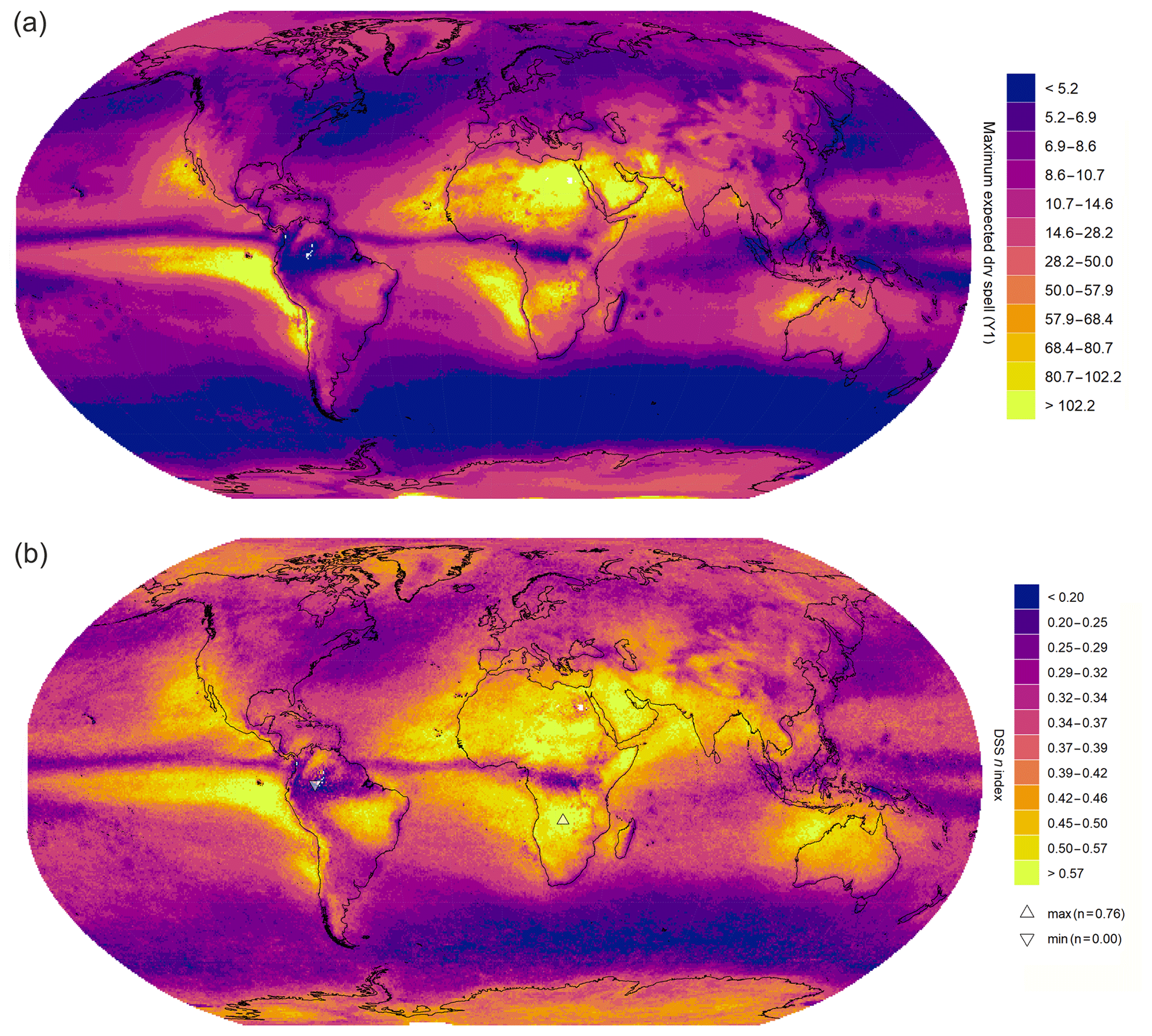
Figure 1Spatial distribution of regularity of the lacunarity, averaging for all DSS events: (a) maximum expected dry spell (Y1) and (b) DSS n index.
More specifically, rainforests like those in the Amazon, the Congo, or southeastern Asia present values of n<0.3. This is consistent with the low values also found for other rainforest zones such as those in Madagascar, Central America, and South America. This is due to the high degree of persistence of very short dry spells, alternating with very frequent wet days. Low values are also provided by the domain regions due to the action of the polar jet streams in both hemispheres. This is the case of the zonal flux in the Southern Ocean and the eastern fringes of North America and Asia.
High values of the index (n>0.4) are presented in the tropical and subtropical regions due to the effect of the subtropical anticyclones, particularly in the deserts. The savannah regions show the highest values of n, which involve a long dry spell followed by shorter dry events. The polar regions score a secondary maximum of n due to the usually long but irregular dry events. Similar spatial results are found if G and Ce are used (Fig. 2), while the Hurst exponent displays noisier patterns around the world, very close to 0.5, as described by other studies for Europe (Martínez et al., 2007; Lana et al., 2010). Most of the cases show values n<0.5; similarly, approximately 80 % of the G values are lower than 0.5. Both results indicate the existence of a noteworthy degree of homogeneity in the distribution of the dry spells along the time series. In fact, the Hurst exponent is close to 0.5 (i.e. the associated fractal dimension could be 1.5), which can be interpreted as an equilibrium between positive and negative autocorrelations.

Figure 2Spatial distribution of other fractal measures applied to dry spells: (a) Hurst exponent, (b) Gini index, and (c) Cantor-based exponent.
3.2 Drought classification
Three main sets can be identified according to the predominance of low (L), medium (M), or high (H) values of the DSS n index: Type S when n<0.3, Type M if n is within the interval (0.3, 0.4), and Type L for n>0.4. For the three main types, it is advisable to distinguish between the alternation with longer (ℓ) or shorter (s) wet events, for example, considering the threshold of three consecutive wet days (Fig. A1). Therefore, six large drought types can be defined based upon the combination of both criteria (Fig. 3):
-
Type Lℓ. This is the occurrence of very short dry spells alternating with longer wet spells. Tropical examples include the main rainforest cores of the world (within the Amazon, the Congo, and southeastern Asia, among others), and subpolar examples include the Southern Ocean and some regions of the North Atlantic and North Pacific oceans.
-
Type Ls. This is the occurrence of very short dry spells alternating with short wet spells. Examples include northeastern America and northeastern Asia, especially Japan.
-
Type Mℓ. These are median dry spells alternating with longer wet spells. Examples include the Arctic Ocean and northern Asia.
-
Type Ms. These are median dry spells alternating with shorter wet spells. Examples include the central area of North America and the temperate regions of the Atlantic and Pacific Oceans.
-
Type Hℓ. This is the occurrence of very long dry spells alternating with long wet events. Examples include the tropical savannah regions of Africa, Mexico, central Brazil, India (monsoon climate), southern China, and northern Australia.
-
Type Hs. This is the occurrence of very long dry spells alternating with short wet events. Examples include all the desert regions around the world, including the eastern fringe of the tropical oceanic areas.
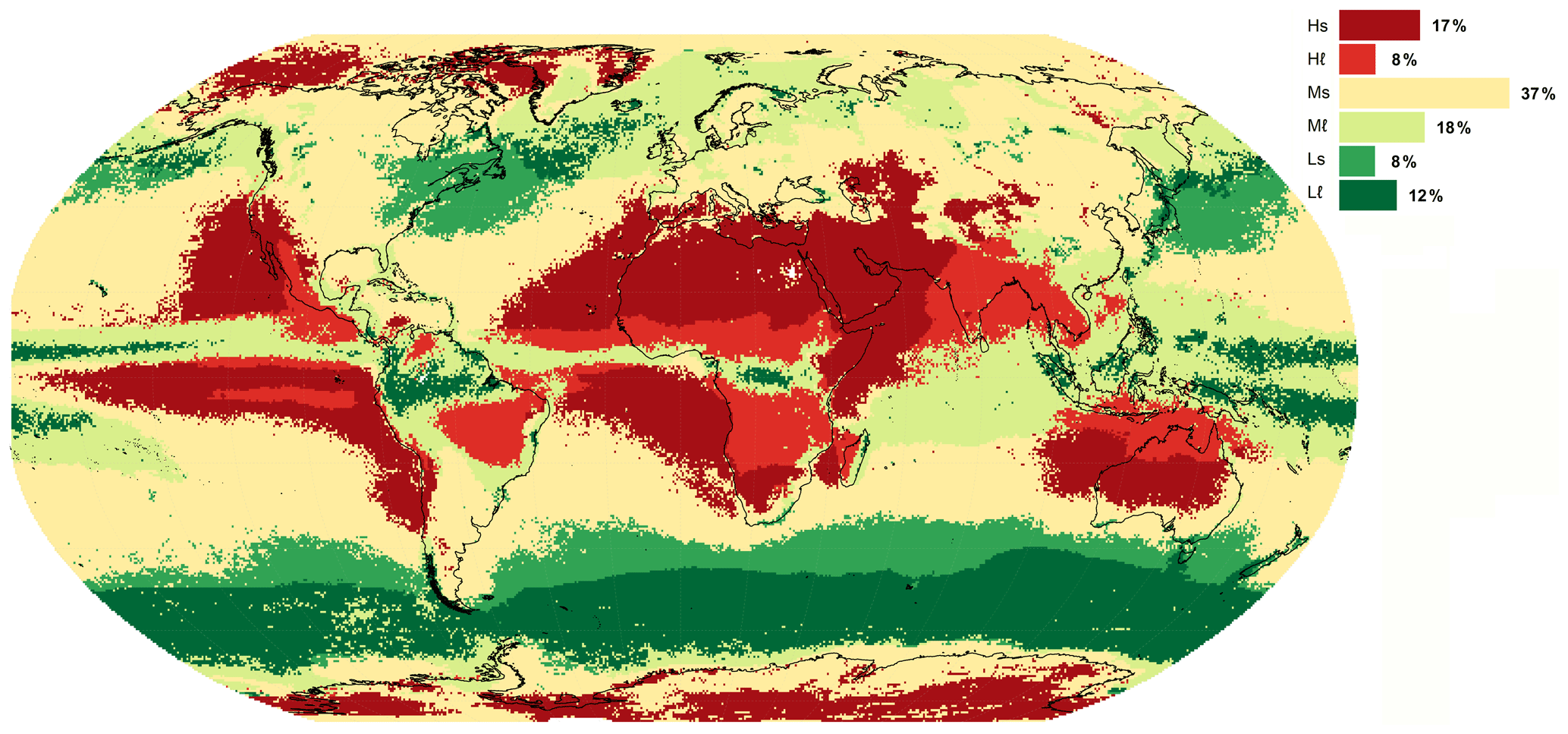
Figure 3Climatic classification of meteorological droughts around the world: regions with low (L), medium (M), or high (H) values of the DSS n index, alternating with longer (ℓ) or shorter (s) wet events.
3.3 Drought lacunarity
Since the total (1-D) length of the Cantor set is zero, the total length of the complementary gaps is equal to 1. That is, following the analogy between the drought duration and the Cantor set lacunarity, the total duration of a dry-spell series approaches 1 when the size of the measurement box is accurate. For instance, one can find dry days in a wet month, and on rainy days, there can be several hours with no rain. If a ground point is used for measurement, the duration of a raindrop hitting the ground (from leading surface to trailing surface) tends towards zero, and thus the dry pauses are distributed paradoxically throughout an entire rainy day.
According to this idea, the dimension of the drought duration is practically 1 (the length of the time series), and the box-counting dimension therefore makes more sense for measuring rainfall duration than for estimating drought duration. However, the lacunarity of the drought can be analysed by means of other measures, such as the Gini index (G) and the Cantor-based exponent (Ce), both of these related to the frequency of dry-spell durations. In particular, the Cantor-based exponent indicates how likely it is to find longer dry spells over time. For instance, if Ce∼0, all dry spells will present similar lengths and therefore the standard deviation will be constant (i.e. extreme values are normally distributed). However, if Ce∼1, the distribution of lengths is similar to the Cantor lacunarity, and the standard deviation will therefore increase over time. In this case, extreme dry spells show a linear increase for longer time series (in the same way that the maximum Cantor gap is set at 1∕3 of the total length), and the Gini index also tends to approach 1. Indeed, the correlation between the G and Ce is R2=0.86 (p value <0.0001) and the approximation Ce=G only provides an error of 10 %, thus reinforcing the lacunar interpretation of the dryness.
The DSS n index provides information on the structure of drought lacunarity, in particular measuring the probability of regularity (if n∼0) or irregularity (if n∼1). Regular values of dry spells indicate that similar dry-spell lengths are usually consecutive. Accordingly, irregular values imply that long dry spells are followed by much shorter dry sequences. It should be kept in mind a high degree of irregularity is correlated with the longest dry spells (Fig. A3).
In short, the time patterns of the dryness of a climate can be characterised in a simple manner by means of the n index. This indicator represents a synthetic DSS, computed by averaging all the DSS events of a considered time series. In each DSS, a relative distribution can be observed of consecutive dry spells and the maximum dry-spell duration. For example, the highest values of the DSS n index (observed in parts of Africa) imply a high accumulation of dry-spell durations with a low number of events considered, whereas the lowest values of the DSS n index (found in the northwestern Amazon) point to a constant and linear accumulation of dry spells presenting the same (short) duration (Fig. A4). The DSS n index therefore provides information on the relative distribution of dry spells, on the longest duration, and on the total accumulated duration. Indeed, the start and end of a synthetic DSS event can be established by the number i of dry-spell events so that the averaged maximum duration Yi is a particular threshold (e.g. 1 d, which is defined as the dry threshold of a DSS event). This idea enables the concept of a DSS event to be employed as an alternative definition of meteorological drought, with diffuse borders that, paradoxically, are well defined by the n index. For instance, if Yi=0 is considered to be drought borders, the total duration of the dryness coincides with the total length of a time series (as the length of the supplementary gaps of the Cantor set). In this case, the difference between one drought and another is given by the decay rate of the maximum dry spell (well measured by the n index).
As in (fractal) wet spells, the behaviour of dryness is self-similar on all timescales – that is to say, dry spells can be used at the daily, monthly, yearly resolution, etc., considering specific dryness thresholds. This is guaranteed by the goodness of fit of the n index model (p value <0.0001). The proposed mathematical definition is complementary to the previous ideas on the persistence of dryness, for example, according to upper-order Markov chains (Lana et al., 2018). Indeed, the order of chains depends on the alternation and frequency of short and long dry spells, as with the rest of the measures (Gini index, Hurst exponent, n index, etc.).
Finally, the main limitation in this study is the possible errors derived from the used precipitation dataset. However, the source errors are generally smaller for the breaks between dry and wet spells because they are not influenced by the absolute precipitation amount.
The datasets from Figs. 1–3 and Fig. A1 can be accessed through Monjo et al. (2019) (https://doi.org/10.5281/zenodo.3247041). The used software code (R programming language) with a point example can be accessed through Monjo et al. (2019) at GitHub: https://github.com/robertmonjo/drought.
As a principal conclusion, the study demonstrates that drought lacunarity can be analysed with the use of self-similarity features obtained from the DSS n index. This measure is useful for characterising the temporal and spatial patterns of drought, which are consistent with the climatic features established worldwide. For instance, localities presenting very frequent wet spells alternating with short dry spells provide low values of the DSS n index (this is the case, for example, in the Amazon, the Congo, and other rainforests). This results from an accumulation of isolated short dry spells, all presenting the same duration. Additionally, places with longer dry spells (such as deserts) scored higher values on the DSS n index. This result is logical because the n index is strongly correlated with the maximum and average lengths of dry spells as well as with the Gini index.
Consequently, we arrived at a second conclusion: the methodology developed can be used to classify typologies of meteorological drought. Indeed, six climate types have been proposed: these result from the combination of three classes of DSS n index values (Type L when n<0.3, Type H for n>0.4, and Type M otherwise) and two sub-classes based on the alternation with longer (ℓ) or shorter (s) wet events. This classification could be useful with regard to monitoring possible changes in drought patterns around the world within the context of climate change (Monjo et al., 2016; Craine et al., 2013; Madakumbura et al., 2019). The third and most important outcome refers to the fact that consideration of dryness lacunarity provides a better understanding of drought duration and helps to predict when droughts start and finish. Further works may use other dataset at a global or regional scale (with more spatial resolution) to analyse past and future climate change (e.g. by using CMIP6 climate models). Moreover, future studies may focus on designing specific indicators to monitor hydrological and agricultural droughts, especially involving datasets on river discharges, soil moisture, water stress, or related damage. In particular, the value of the DSS n index is related to the effective duration (according to borders determined by a threshold of the minimum expected dry spell). Indeed, the best analogy with regard to understanding the features of the DSS is Cantor lacunarity; i.e. total dry spells are almost equal to the length of the entire series (in the same manner that the total length of Cantor voids is equal to 1). The methodology presented here provides a set of potentialities: from analysing the change of drought regimes to feeding indicators for monitoring impacts on agricultural or hydrological droughts, with the possibility of using data with a higher spatial resolution.
Note that the mean dry spell (MDS) and the mean wet spell (MWS) are geographically distributed, with a strong correspondence between the high (low) values of the one and the low (high) values of the other. A general zonal pattern is observed, albeit with a clear dissymmetry between the western facades of the continents and the eastern oceans, in tropical–subtropical latitudes, with high values of the MDS (low values of the MWS), and their responses, with low (high) values. The highest values of the MDS are concentrated in the tropical–subtropical zones, especially in the Sahara and its continuation in the Arabian Desert, in the Persian Gulf and the waters of the Indian waters of the Indian Ocean, in lower California, in northern Chile, on the coast of Peru and its waters, in the Atlantic Ocean off the coast of Namibia, and towards the west–northwest of Australia (bordering with Antarctica). The most similar values between both indices, specifically with high values in both, are observed in the Asia-Pacific region (monzonic region), reflecting the division of the year into two halves, the rainy summer, with long rains, and the dry winter, with an absence of precipitation for many days in a row. This pattern can be detected in other areas presenting a humid–dry tropical climate, such as the southernmost area of the Sahel, northeastern Brazil, an area in Africa (south of the Equator), and northern Australia. The SW–NE diagonals of mid-latitudes with decreasing values of the MDS in the Atlantic and the Pacific are clearly appreciated, according to the westerlies and the track of the low-pressure systems.
For instance, let be a time series of consecutive dry spells. A DSS event is built around the minimum value (D0=1) as (10, 4, 8, 10, 20). Subsequently, maximum accumulated dry durations are , and the maximum averaged dry durations are , which can be fitted over the number of events (i) according to Eq. (3).
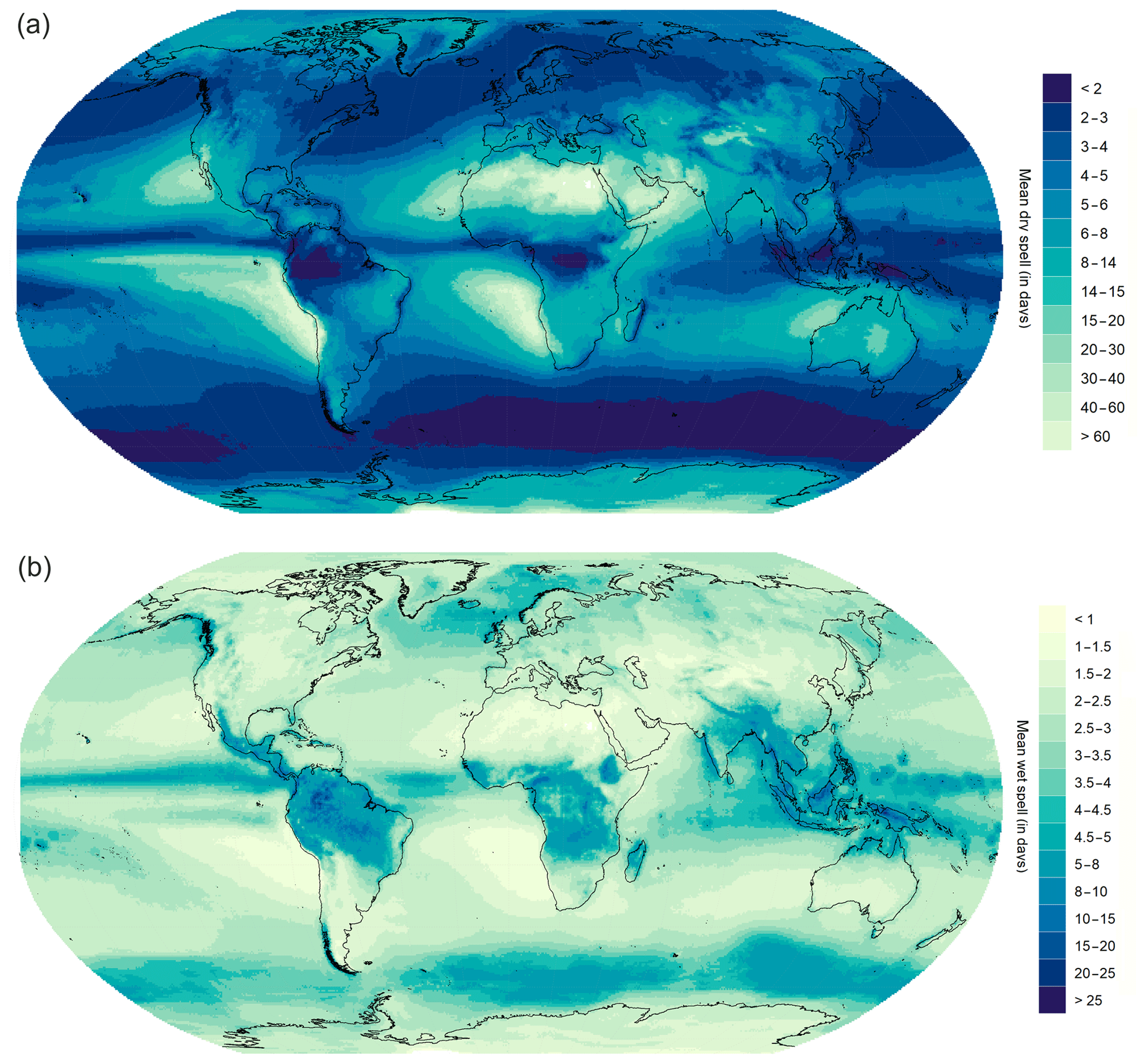
Figure A1Spatial distribution of mean dry spell (a) and mean wet spell (b) at a spatial resolution of according to the MSWEP dataset (1979–2016).
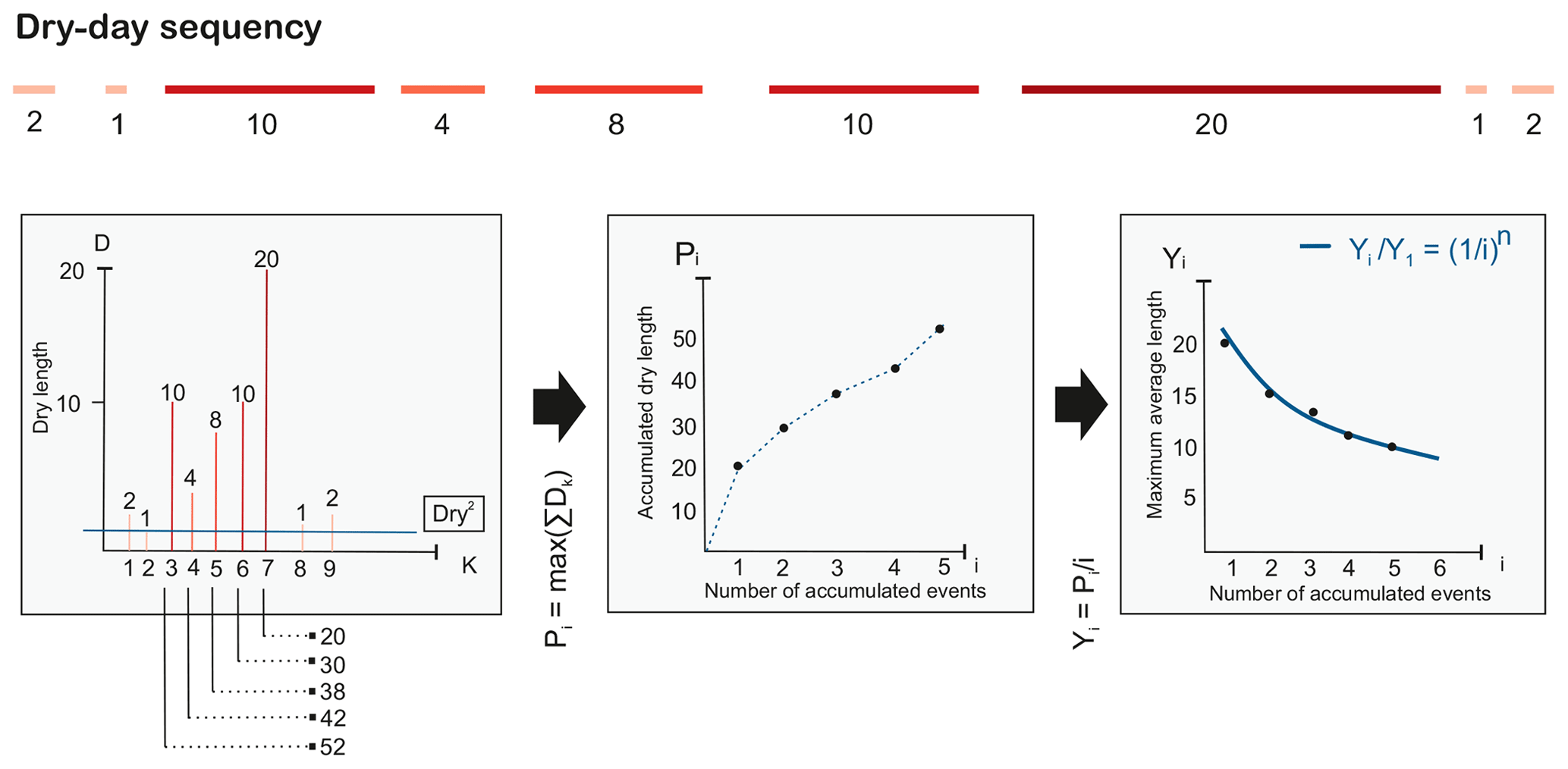
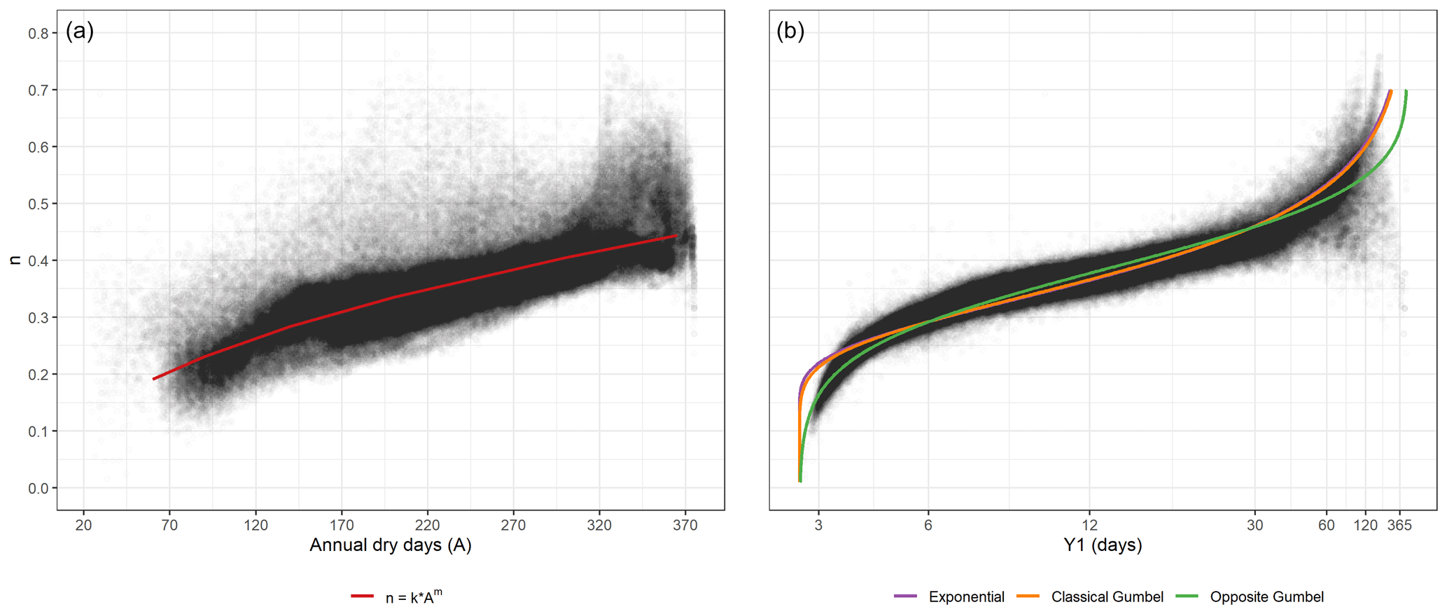
Figure A3Statistical relationship between (a) annual dry days (A) and the DSS n index and (b) maximum expected dry spell (Y1) and the DSS n index.
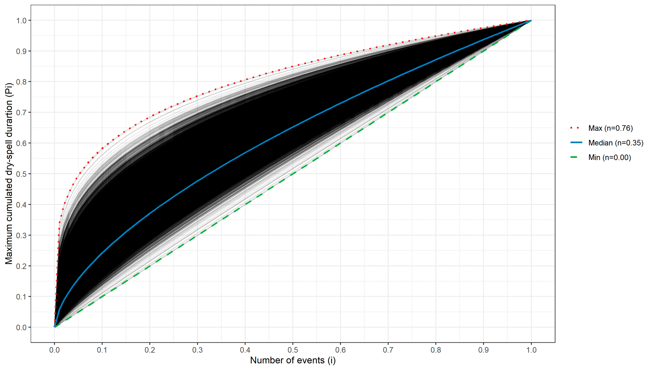
Figure A4Fitted curves of DSS events (Eq. 4), according to the maximum accumulated dry-spell duration (Pi) over the number of events considered (i), both normalised according to the total values.
The fitted parameters for the first curve are k=0.02811(3) and m=0.4677(8) (R2=0.67, p value <0.0001). In the second panel, the fitted curves are exponential (α1=0.997(3), , AIC ≈ BIC , R2=0.91, p value <0.0001), Gumbel (α2=1.225(3), , AIC ≈ BIC , R2=0.88, p value <0.0001), and opposite Gumbel (α3=3.829(2) and , AIC , R2=0.87, p value <0.0001), according to the Eqs. (6)–(8).
Note that the minimum DSS n index corresponds to the Amazon, where almost every DSS event lasts for only 1 d, and the accumulation of dry spells (Yi) is therefore very regular. Furthermore, the maximum n index (close to the Zambezi River) represents an average DSS event with a maximum dry spell of 33 % of the total accumulated dry-spell length (most of the entire time series) and successive dry spells with shorter durations (as in the Cantor gaps).
The Cantor-based exponent and the n index were designed by RM, and all the calculus and figures were created by DR, while RM and JMV interpreted the results and RM wrote the paper. All authors read and approved the final paper.
The authors declare that they have no conflict of interest.
We are grateful for the support provided by the RESCCUE project, which received funding from the European Research Council under the European Union's Horizon 2020 research and innovation programme (grant agreement no. 700174). We also wish to acknowledge the support received from the Spanish projects CGL2017-83866-C3-2-R and Climatology Group 2017 SGR 1362. We appreciate the interest in our research shown by the Water Research Institute of the University of Barcelona and by the Department of Algebra, Geometry and Topology of the Complutense University of Madrid.
This research has been supported by the European Research Council (RESCCUE (grant no. 700174)) and the Spanish Ministry of Science, Innovation and Universities (grant no. CGL2017-83866-C3-2-R).
This paper was edited by Alexander Gelfan and reviewed by Hasan Tatli and Serguei G. Dobrovolski.
Beck, H. E., van Dijk, A. I. J. M., Levizzani, V., Schellekens, J., Miralles, D. G., Martens, B., and de Roo, A.: MSWEP: 3-hourly 0.25∘ global gridded precipitation (1979–2015) by merging gauge, satellite, and reanalysis data, Hydrol. Earth Syst. Sci., 21, 589–615, https://doi.org/10.5194/hess-21-589-2017, 2017. a
Bezruchko, B. and Smirnov, D.: Extracting Knowledge From Time Series: An Introduction to Nonlinear Empirical Modeling, Springer, 2010. a
Boeing, G.: Visual analysis of nonlinear dynamical systems: chaos, fractals, self-similarity and the limits of prediction, Systems, 4, 37, https://doi.org/10.3390/systems4040037, 2016. a
Craine, J., Ocheltree, T., Nippert, J., Towne, E., Skibbe, A., Kembel, S., and Fargione, J.: Global diversity of drought tolerance and grassland climate-change resilience, Nat. Clim. Change, 3, 63–67, 2013. a
Crausbay, S. D., Ramirez, A. R., Carter, S. L., Cross, M. S., Hall, K. R., Bathke, D. J., Betancourt, J. L., Colt, S., Cravens, A. E., Dalton, M. S., Dunham, J. B., Hay, L. E., Hayes, M. J., McEvoy, J., McNutt, C. A., Moritz, M. A., Nislow, K. H., Raheem, N., and Todd, S.: Defining ecological drought for the twenty-first century, B. Am. Meteorol. Soc., 98, 2543–2550, 2017. a
Dayeen, F. and Hassan, M.: Multi-multifractality, dynamic scaling and neighbourhood statistics in weighted planar stochastic lattice, Chaos Soliton. Fract., 91, 228–234, https://doi.org/10.1016/j.chaos.2016.06.006, 2016. a
Feder, J.: Fractals, Plenum press, New York, Springer USA, 284 pp., https://doi.org/10.1007/978-1-4899-2124-6, 1988. a, b
Feng, D.-J., Rao, H., and Wang, Y.: Self-similar subsets of the Cantor set, Adv. Math., 281, 857–885, https://doi.org/10.1016/j.aim.2015.06.002, 2015. a
Gaspard, P.: Chaos, Scattering and Statistical Mechanics, Cambridge University Press, 2005. a
Hou, W., Yan, P.-C., Li, S.-P., Tu, G., and Hu, J.-G.: Application of long-range correlation and multi-fractal analysis for the depiction of drought risk, Chinese Phys. B, B25, 019201, https://doi.org/10.1088/1674-1056/25/1/019201, 2016. a
Imre, A. R. and Bogaert, J.: The Minkowski-Bouligand dimension and the interior-to-edge ratio of habitats, Fractals, 14, 49–53, 2006. a
Kuznetsov, N. V.: The Lyapunov dimension and its estimation via the Leonov method, Phys. Lett. A, A.380, 2142–2149, 2016. a
Lana, X., Martínez, M. D., Serra, C., and Burgueño, A.: Complex behaviour and predictability of the European dry spell regimes, Nonlin. Processes Geophys., 17, 499–512, https://doi.org/10.5194/npg-17-499-2010, 2010. a, b
Lana, X., Martínez, M., Burgueño, A., Serra, C., Martín-Vide, J., and Gómez, L.: Spatial and temporal patterns of dry spell lengths in the Iberian Peninsula for the second half of the twentieth century, Theor. Appl. Climatol., 91, 99–116, 2018. a, b
Lucena, L. R. R. D., Júnior, S. F. A. X., Stosic, T., and Stosic, B.: Lacunarity analysis of daily rainfall data in Pernambuco, Brazil, Acta Scientiarum Technology, 40, E36655, https://doi.org/10.4025/actascitechnol.v40i4.36655, 2018. a, b
López de la Franca Arema, N., Sanchez, E., Losada, T., Dominguez, M., Romera, R., and Gaertner, M.: Markovian characteristics of dry spells over the Iberian Peninsula under present and future conditions using ESCENA ensemble of regional climate models, Clim. Dynam., 45, 661–677, 2015. a
Madakumbura, G. D., Kim, H., Utsumi, N., Shiogama, H., Fischer, E. M., Seland, O., Scinocca, J. F., Mitchell, D. M., Hirabayashi, Y., and Oki, T.: Event-to-event intensification of the hydrologic cycle from 1.5∘C to a 2∘C warmer world, Sci. Rep., 9, 3483, https://doi.org/10.1038/s41598-019-39936-2, 2019. a
Mandelbrot, B.: How long is the coast of Britain? Statistical self-similarity and fractional dimension, Science, 156, 636–638, 1967. a
Mandelbrot, B.: Self-affinity and fractal dimension, Phys. Scripta, 32, 257–260, 1985. a, b
Martín-Vide, J. and Gomez, L.: Regionalization of Peninsular Spain based on the length of dry spells, Int. J. Climatol., 19, 537–555, 1999. a
Martínez, M. D., Lana, X., Burgueño, A., and Serra, C.: Lacunarity, predictability and predictive instability of the daily pluviometric regime in the Iberian Peninsula, Nonlin. Processes Geophys., 14, 109–121, https://doi.org/10.5194/npg-14-109-2007, 2007. a, b, c
Meseguer-Ruiz, A., Olcina, J., Sarricolea, P., and Martin-Vide, J.: The temporal fractality of precipitation in mainland Spain and the Balearic Islands and its relation to other precipitation variability indices, Int. J. Climatol., 37, 849–860, 2017. a
Monjo, R.: Measure of rainfall time structure using the dimensionless n-index, Clim. Res., 67, 71–86, 2016. a, b, c
Monjo, R. and Martin-Vide, J.: Daily precipitation concentration around the world according to several indices, Int. J. Climatol., 36, 3828–3838, 2016. a, b, c
Monjo, R., Gaitán, E., Pórtoles, J., Ribalaygua, J., and Torres, L.: Changes in extreme precipitation over Spain using statistical downscaling of CMIP5 projections, Int. J. Climatol., 36, 757–769, 2016. a
Monjo, R., Royé, D., and Martin-Vide, J.: Drought lacunarity around the world and its classification (Version v0.1) [Data set], Zenodo, https://doi.org/10.5281/zenodo.3247041, 2019. a, b, c
Olsson, J., Niemczynowicz, J., Berndtsson, R., and Larson, M.: An analysis of the rainfall time structure by box counting—some practical implications, J. Hydrol., 137, 261–277, 1992. a
Plotnick, R. E., Gardner, R. H., Hargrove, W., Prestegaard, K., and Perlmutter, M.: Lacunarity analysis: A general technique for the analysis of spatial patterns, Phys. Rev. E, 53, 5461–5468, 1996. a
Sakhr, J. and Nieminen, J. M.: Local box-counting dimensions of discrete quantum eigenvalue spectra: Analytical connection to quantum spectral statistics, Phys. Rev. E, E97, 030202, https://doi.org/10.1103/PhysRevE.97.030202, 2018. a
Sen, Z.: Wadi Hydrology, CRC Press, 368 pp., 2008. a
Tatli, H.: Detecting persistence of meteorological drought via the Hurst exponent, Meteorol. Appl., 22, 763–769, 2015. a
Vicente-Serrano, S., Van der Schrier, G., Beguería, S., Azorin-Molina, C., and Lopez-Moreno, J.: Contribution of precipitation and reference evapotranspiration to drought indices under different climates, J. Hydrol., 426, 42–54, 2015. a
Vicente-Serrano, S. M., Beguería, S., and López-Moreno, J.: A Multi-scalar drought index sensitive to global warming: The Standardized Precipitation Evapotranspiration Index – SPEI, J. Climate, 23, 1696–1718, 2010. a
Wilhite, D. and Glantz, M.: Understanding the Drought Phenomenon: The Role of Definitions, Water Int., 10, 111–120, 1985. a
Wilkinson, M., Pradas, M., Huber, G., and A., P.: Lacunarity exponents, J. Phys. A-Math. Theor., 52, 115101, https://doi.org/10.1088/1751-8121/ab0349, 2019. a
Yu, S., Piao, X., Hong, J., and Park, N.: Bloch-like waves in random-walk potentials based on supersymmetry, Nat. Commun., 6, 8269, https://doi.org/10.1038/ncomms9269, 2015. a