the Creative Commons Attribution 4.0 License.
the Creative Commons Attribution 4.0 License.
 | 17 Mar 2020
Marine carbonyl sulfide (OCS) and carbon disulfide (CS2): a compilation of measurements in seawater and the marine boundary layer
Sinikka T. Lennartz
Christa A. Marandino
Marc von Hobe
Meinrat O. Andreae
Kazushi Aranami
Elliot Atlas
Max Berkelhammer
Heinz Bingemer
Dennis Booge
Gregory Cutter
Pau Cortes
Stefanie Kremser
Cliff S. Law
Andrew Marriner
Rafel Simó
Birgit Quack
Günther Uher
Huixiang Xie
Xiaobin Xu
Carbonyl sulfide (OCS) and carbon disulfide (CS2) are volatile sulfur gases that are naturally formed in seawater and exchanged with the atmosphere. OCS is the most abundant sulfur gas in the atmosphere, and CS2 is its most important precursor. They have attracted increased interest due to their direct (OCS) or indirect (CS2 via oxidation to OCS) contribution to the stratospheric sulfate aerosol layer. Furthermore, OCS serves as a proxy to constrain terrestrial CO2 uptake by vegetation. Oceanic emissions of both gases contribute a major part to their atmospheric concentration. Here we present a database of previously published and unpublished (mainly shipborne) measurements in seawater and the marine boundary layer for both gases, available at https://doi.org/10.1594/PANGAEA.905430 (Lennartz et al., 2019). The database contains original measurements as well as data digitalized from figures in publications from 42 measurement campaigns, i.e., cruises or time series stations, ranging from 1982 to 2019. OCS data cover all ocean basins except for the Arctic Ocean, as well as all months of the year, while the CS2 dataset shows large gaps in spatial and temporal coverage. Concentrations are consistent across different sampling and analysis techniques for OCS. The database is intended to support the identification of global spatial and temporal patterns and to facilitate the evaluation of model simulations.
- Article
(715 KB) - Full-text XML
- BibTeX
- EndNote


Carbonyl sulfide (OCS) is the most abundant sulfur gas in the atmosphere with a tropospheric mixing ratio around 500 ppt (Kremser et al., 2016). Carbon disulfide (CS2) is a short-lived sulfur gas, which is oxidized within hours to days. Because OCS is a major product of this oxidation, with a yield of 82 % (i.e., 82 molecules of OCS produced from 100 CS2 molecules), CS2 oxidation is a major source of OCS in the atmosphere.
Atmospheric mixing ratios of OCS show larger annual than interannual variations (Montzka et al., 2007). Small negative trends between 10 % and 16 % decrease, derived from firn air and flask measurements, have been reported for the 1980 to 2000 period (Montzka et al., 2004). Since 2001, small positive trends <10 % per decade were derived from OCS observations in the Southern Hemisphere (Kremser et al., 2015).
Due to its long tropospheric lifetime of 2–7 years, OCS is entrained into the stratosphere. In volcanically quiescent periods, OCS (and indirectly CS2) is thought to be a major contributor to stratospheric sulfate aerosols that influence the radiative budget of the Earth (Crutzen, 1976; Brühl et al., 2012). In addition, OCS can be used as a proxy to quantify the CO2 uptake of plants (gross primary production), which is a major source of uncertainty in climate modeling (Whelan et al., 2018). Both scientific interests benefit from a well-constrained atmospheric budget. OCS and CS2 are produced naturally in the ocean, and their oceanic emissions contribute substantially to their atmospheric concentrations (Chin and Davis, 1993; Watts, 2000; Kremser et al., 2015).
Oceanic source estimates of OCS and its precursor CS2 still contain large uncertainties (Kremser et al., 2016; Whelan et al., 2018). Current efforts to model surface concentrations of OCS in seawater diverge in their results (Launois et al., 2015; Lennartz et al., 2017). Most measurements of oceanic OCS and CS2 were performed in the 1980s and 1990s, and data are often not available or stored inaccessibly, hampering model evaluation or analysis of global spatial and temporal concentration patterns. Therefore, a combined database for marine measurements of OCS and CS2 has been given high priority in a recent review on using OCS as a tracer for gross primary production (Whelan et al., 2018). Here, we aim to provide such a comprehensive database by compiling previously reported, as well as unpublished data, from corresponding authors of the original studies or via digitalization from pdf documents. Both OCS and CS2 show a pronounced variability in seawater, which implies a need for highly resolved observations. Therefore, we pay special attention to the temporal resolution of measurements in the database. The seasonal variability is a direct result of the marine cycling of both gases. Photochemical reactions involving chromophoric dissolved organic matter (CDOM) lead to the formation of OCS, as does a light-independent production pathway (Ferek and Andreae, 1984; Weiss et al., 1995a; Von Hobe et al., 2001). OCS is efficiently hydrolyzed in seawater. The temperature dependence of the hydrolysis reaction leads to high degradation rates in warm waters (Elliott et al., 1989; Radford-Knoery and Cutter, 1994; Kamyshny et al., 2003). The efficient photochemical production and fast degradation in warm waters result in strong diurnal and seasonal cycles of OCS in the surface ocean (Kettle et al., 2001; Ulshöfer et al., 1995). CS2 is photochemically produced in seawater as well, but diurnal cycles are not as pronounced due to lower efficiency of the sink processes. Concentrations of CS2 and OCS in seawater differ strongly depending on the time of day and season measured. To facilitate interpretation of concentration measurements on larger scales in relation to the processes described above, ancillary data coinciding with trace gas measurements are also reported if available, such as meteorological or physical seawater properties. The database is described with respect to number of data, range, and patterns of concentrations; analytical methods; temporal and spatial coverage; and sampling frequency for each dataset.
2.1 Data collection
Data were obtained either from authors of previous studies directly or digitalized with a web-based digitalization tool from pdf documents. Web of Science was searched for the key words “carbonyl sulfide” (both sulfide and sulphide), “carbon disulfide” (both sulfide and sulphide) in connection with “ocean” or “seawater”. When data could not be obtained directly from authors, relevant figures were identified and digitalized with the WebPlotDigitizer Automeris (https://apps.automeris.io/wpd/, last access: January 2019). When digitalizing the data from documents, concentration data were rounded to the integer to account for uncertainty in the digitalization method introduced, e.g., by misalignment of the axes in case of old scanned pdf documents. Here we include only shipborne measurements or observations from stations with a marine signal (i.e., research platforms in the North Sea, ID15; on Amsterdam Island, ID6; and in Bermuda, ID39). For atmospheric OCS data from aircraft campaigns or continental time series stations, i.e., HIAPER-Pole-to-Pole-Observations (HIPPO, Montzka, 2013), Atmospheric Tomography Mission (ATom, Wofsy et al., 2018), and the NOAA time series stations from the Earth System Research Laboratory – Global Monitoring Division (NOAA-ESRL, Montzka, 2004, Montzka et al., 2007), we refer to the respective repositories accessible online (HIPPO: https://www.eol.ucar.edu/field_projects/hippo, last access: 1 August 2019; ATom: https://espo.nasa.gov /atom/content/ATom, last access: 1 August 2019; NOAA-ESRL: https://www.esrl.noaa.gov/gmd/, last access: 1 August 2019).
Concentration data were converted to the unit picomole OCS∕CS2 L−1, accounting for molar masses of sulfur (32.1 g), OCS (60 g), and CS2 (76.1 g). Data were collected together with the following metadata (if reported in the original publication or otherwise available):
-
latitude of measurement;
-
longitude of measurement;
-
date, including year, month, day, hour, and minute;
-
name of the cruise and/or ship;
-
contributor;
-
main reference for data;
-
method description;
-
main reference for method;
-
sample depth;
-
any ancillary data (meteorological, physical, biological data);
-
flag describing the sampling resolution (see Table 1).
It should be noted that several commonly used materials, such as any rubber parts, may lead to contaminations when measuring OCS and CS2. A non-exhaustive list of problematic materials is available here: http://www.cosanova.org/materials-to-avoid.html (last access: February 2019). We paid attention to the method description of each dataset, and data were only included when blank measurements are reported or the description of the material was provided (e.g., Teflon used). An overview of the dataset is provided in Table 2 (methods) and Table 3 (sampling details). A filling value of −999 was introduced for concentrations below the respective detection limit of each individual dataset. Missing additional data (physicochemical parameters, meteorological parameters, etc.) was filled with NaN (not a number) to facilitate readability in data handling software. The database can be accessed at the data repository PANGAEA (https://doi.org/10.1594/PANGAEA.905430, Lennartz et al., 2019). Available additional data are listed in Table 4.
Table 1Flags used to describe sampling frequency of each individual dataset.

2.2 Trace gas analysis
2.2.1 Carbonyl sulfide in seawater
Carbonyl sulfide (OCS) concentrations in seawater were commonly measured with a method to separate gaseous OCS from the seawater connected to a detection system. Two main principles were applied to separate OCS from seawater: (1) purging the water sample with an OCS-free gas to transfer the total dissolved OCS into the gas phase or (2) using an equilibrator, where a gas phase is brought into equilibrium with the seawater sample. The OCS concentration in water is then calculated using Henry's law and the temperature during the equilibration process. Sampling using method 1 is usually performed discretely and has sometimes been replaced by method 2 with automated (semi)continuous sampling with a sampling resolution of <15 min since 2015 (Ulshöfer et al., 1995; Von Hobe et al., 2008; Lennartz et al., 2017). OCS detection in discrete samples used gas chromatography (GC). Most GCs were then coupled to a flame photometric detector (GC-FPD) or, less frequently, to an electron capture detector (GC-ECD). Commonly, samples were cryogenically pre-concentrated (e.g., with liquid N2) prior to injection into the GC. A new technique using off-axis integrated cavity output spectroscopy (OA-ICOS) has only recently been developed to continuously measure dissolved OCS in seawater with the use of an equilibrator (Lennartz et al., 2017).
For the majority of the samples in the database, the precision was reported to be better than 10 %, and the limit of detection are around 2 pmol L−1 (see Table 2 for details on individual datasets). The instability of OCS in water makes the comparison with liquid standards difficult, which is why most of the studies used permeation tubes to calibrate their instruments. Unfortunately, no intercalibration between cruises is reported (see Sect. 3.1 for a discussion of quality control of the data).
Table 2Description of all cruises or campaigns contributing measurements to this database. Cruises are given a unique ID for identification. Reference refers to the publication where the data were reported first. Methods are reported using the same specifications and level of detail as given in the original publication. Specifications for analytical methods are listed together with the method referenced in the main reference: di (or) stands for digitalized (original) data, S stands for sampling, An stands for analysis, Det stands for details, and R stands for reference of instrumentation. Letters in the last column indicate direct comparability of the datasets, as studies were performed with either identical analytical systems (i.e., same method reference) or performed by the same laboratory through further development of analytical systems (i.e., different method reference) but intercomparison within laboratory.
2.2.2 Carbonyl sulfide in the marine boundary layer
Quantifying the OCS concentration in the sampled gas is performed in a similar way with the same analytical systems, as described in Sect. 2.2.1 for dissolved concentration measurements. The database consists mainly of shipborne measurements but includes measurements from two land-based stations with strong marine influence. These two datasets are (1) ID6 from Amsterdam Island in the Southern Ocean and (2) ID39 from Tudor Hill, Bermuda.
The majority of studies used a GC-FPD system; GC-ECD and OA-ICOS were less frequently used. Detection limits and precision were comparable or identical to seawater measurements described in the previous section. Details on each individual method are listed in Table 2. Quantification was achieved with standards produced from permeation tubes and from gas cylinders from various manufacturers (see Table 2 for specifications of individual studies). No intercalibration for the complete database is available.
2.2.3 Carbon disulfide in seawater
Sampling of carbon disulfide (CS2) was performed discretely from both continuously pumped water and containers such as Niskin bottles. Concentrations of CS2 were measured with a sampling frequency of up to 15 min. Most frequently, a GC-MS system was used; GC-FPD was less common. Prior to the injection in the GC, samples were either purged with CS2-free gas, and a cooled trap was used for preconcentration (purge+trap system), or the gas and liquid phase were brought to equilibrium with an equilibrator. Detection limits ranged down to 1 pmol L−1, and the precision was around 3 %–5 % (see Table 2 for specification of the individual datasets). Standard measurements include permeation tubes or liquid standards prepared in ethylene glycol, but no intercalibration has been reported.
2.2.4 Carbon disulfide in the marine boundary layer
Samples were commonly taken discretely from the vessel's deck, directly into air canisters, or sampled directly from air drawn with tubing into the laboratory. Altitudes where samples were taken ranged from 10–25 m. The detection of CS2 in the gas phase was similar to the analytical methods described in the Sect. 2.2.3, without the step of purging the gas out of the water. GC-MS or GC-FPD were used for detection. As described above, detection limits range down to 1 ppt, and the precision is ∼3 %–5 % (see Table 2 for specification of the individual datasets). Standards were either permeation tubes or gas cylinders, detailed in Table 2.
All datasets included here provide some means of quality control, and calibration procedures including primary gravimetric standards from permeation tubes or by certified gas standards are described in the original publications. However, the database compiled here includes measurements made by different laboratories and thus different measurement systems. One limitation of the database is the missing intercalibration across these different measurement systems. Since many of these systems were built and deployed in the 1990s and no longer exist, such an intercalibration is not possible anymore. We strongly recommend undertaking efforts for intercalibration across laboratories for future oceanic measurements of OCS and CS2. Since no practical quality control is possible, we assess the quality of the database by its internal consistency.
3.1 Carbonyl sulfide in seawater
Measurements of OCS in seawater were collected from 32 cruises, resulting in 7536 individual measurements (Fig. 1, Tables 2 and 3). OCS concentrations were measured in the picomolar range in the surface and subsurface ocean, with a mean concentration of 32.3 pmol L−1 (n=7536, Fig. 2a), ranging from below the detection limit to 1466 pmol L−1 in the Rhode Island river estuary.
Figure 1Tracks of all cruises with OCS and/or CS2 measurements included in the database (points depict stationary measurements). Labels indicate the cruise ID (compare Table 1).
The majority of measurements were made in the Atlantic Ocean, with the least being taken from the Indian Ocean. No measurements are available for the Arctic Sea. The sampling was heavily biased towards surface ocean measurements shallower than 10 m depths, and only a few measurements (<3 %) were obtained from concentration profiles in the water column (144 measurements). The available profiles range down to a water depth of 2000 m (Table 3). Reporting the sampling depth is critical for photochemically produced substances such as OCS and the penetration depths of UV light, and hence the photoproduction varies spatially and temporally. Samples that were obtained from depths shallower than 10 m are referred to as “surface samples”, and most of them were obtained at a depth of 3–5 m. Maintaining a continuous water supply despite water level changes by waves on a moving vessel is a challenge and currently hinders continuous sampling at shallower depths. Profile measurements from the North Atlantic indicated that differences in concentration within the surface of the mixed layer <10 m are in a range of about 5 pmol L−1 (Cutter et al., 2004) but might potentially become larger with surface stratification and high irradiation (Fischer et al., 2019).
Table 3Quantitative sampling details for each individual dataset: no. is the number of samples, depth and height are water depth below sea surface and height above sea surface, t.r. is the flag for temporal resolution (see Table 1), mbl is the marine boundary layer, and t.d. is the top deck (height not specified).
* Original paper in sampling frequency of seconds, averaged for this database.
OCS measurements were reported at 12 min to monthly resolution (Fig. 3e). Hence, the majority of the database has the required temporal resolution to cover the full range of the diurnal variation, i.e., a measurement interval of 4 h or less is needed to minimize averaging errors due to interpolation.

Figure 2Georeferenced data for (a) surface ocean OCS concentrations, (b) marine boundary layer OCS mixing ratios, (c) surface ocean CS2 concentrations, and (d) marine boundary layer CS2 mixing ratios. Only surface data (shallower than 10 m) are shown.
Figure 3Overview of the OCS datasets: Boxplots of concentrations per latitudinal bin for (a) water and (b) marine boundary layer measurements. Blue boxes show range of 25 and 75 percentile, horizontal bar indicates the median, and red crosses show outliers. The seasonal variation averaged over all years for (c) water and (d) marine boundary layer (note that in panel c and d, red indicates Northern Hemisphere data, whereas light blue indicates Southern Hemisphere data). Note that measurements >150 pmol L−1 were excluded from these statistics (i.e., coastal samples). Numbers of days with observations for temporal resolution from minute-scale to annually for (e) water and (f) marine boundary layer measurements. (Note that for the boxplots in a and b, only completely georeferenced data were included). NH stands for Northern Hemisphere, and SH stands for Southern Hemisphere.
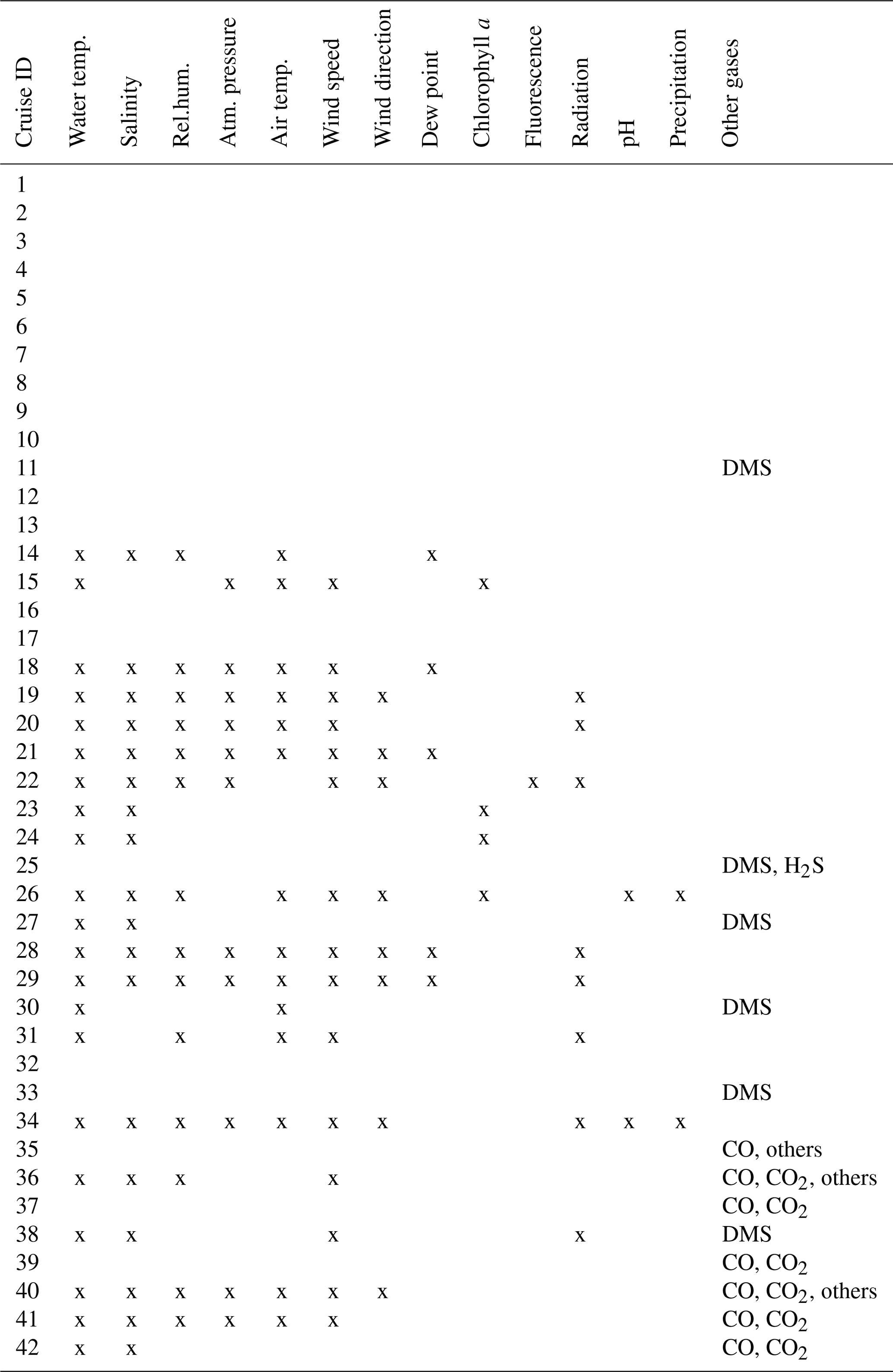
Table 4Ancillary information available for the individual datasets. Physicochemical and meteorological data (water temperature, salinity, relative humidity, atmospheric pressure at sea level, wind speed, absolute wind direction, dew point temperature, chlorophyll a concentration, fluorescence, radiation, pH, and precipitation) are directly included in the database. Availability of other trace gas measurements is indicated, but the data are not included in the database (others, available upon request).
The global variability of the available measurements shows the lowest concentrations in tropical and subtropical waters, especially compared to concentrations at higher latitudes of the Southern Hemisphere (Fig. 3a). The pattern of highest OCS concentrations in coastal and shelf regions has been reported for individual datasets (Cutter and Radford-Knoery, 1993) but is also recognizable in this global database. In particular, the data from cruise ID10 (Cutter and Radford-Knoery, 1993), which covers estuaries and shelves, is 10–1000-fold higher than in oligotrophic warm waters (Fig. 4a). This pattern is also evident in elevated concentration in the North Sea (Uher and Andreae, 1997), the Mediterranean Sea (Ulshöfer et al., 1996) and the coastal waters of Amsterdam Island in the Indian Ocean (Mihalopoulos et al., 1992). Concentration profiles in the water column show a typical photochemical behavior and decrease with depth, although subsurface peaks occur occasionally (Von Hobe et al., 1999; Cutter et al., 2004; Lennartz et al., 2017). Despite the still limited size of the database, it already covers a large part of the global variability, as it includes measurements from a variety of different biogeochemical regimes, i.e., from oligotrophic waters (Cutter et al., 2004; Lennartz et al., 2017; Von Hobe et al., 2001) to higher trophic stages in shelf (Uher and Andreae, 1997), estuary (Cutter and Radford-Knoery, 1993), and upwelling regions (Ferek and Andreae, 1983; Mihalopoulos et al., 1992; Von Hobe et al., 1999; Lennartz et al., 2017).
The annual pattern illustrated in Fig. 3c is different for the Southern Hemisphere and Northern Hemisphere. The lowest median concentrations in the Southern Hemisphere are present during austral winter months and increase up to five times during austral summer. In the Northern Hemisphere, the lowest concentrations are present during late boreal summer (August, September, October) and late boreal winter (January, February, March). The range of observed concentrations is similar for both hemispheres. Compared to the spatial pattern in Fig. 3a, the seasonal variability in the database is larger than the spatial variability.
Figure 4a illustrates the concentration range of each dataset for OCS in seawater. The internal consistency of the database is supported by (1) the variation in concentration in this database being consistent with the current process understanding and thus reflecting actual variability. The majority of the global measurements (60 %) fall into a very narrow range of 8.7–43.0 pmol L−1, and outliers of this 20–80 percentile range are explicable by location or time of measurement. For example, OCS concentrations during cruise ID2, ID10, ID13, and ID19 were much higher than observed by other cruises (Fig. 4), which can be explained by the location of Chesapeake Bay (ID2, ID13), the Petaquamscutt estuary (ID 10), and the North Sea (ID19) in shelf areas or close to estuaries, where high CDOM abundance enhances photochemical production and increases concentration. An example for a particularly low concentration is cruise ID18, which took place during winter. The authors refer the low concentration as due to low photoproduction at that time (Ulshöfer et al., 1995). (2) Measurements obtained from cruises that cover a similar temporal and spatial area yield comparable results, such as cruises ID3 and ID4 (Pacific Ocean); cruises ID27 and ID28 (Atlantic transects; or cruises ID20, ID26, and ID32 from the North Atlantic (Fig. 4). (3) Reported OCS concentrations in seawater and the marine boundary layer are consistent across different laboratories and methods. The introduction of new methods, e.g., OA-ICOS (cruiseID 36 and 39), yields results that are comparable to previous measurements using GC-FPD. To facilitate comparison of individual datasets, they are grouped according to the analysis system used in Table 2 (capital letters in last table column).
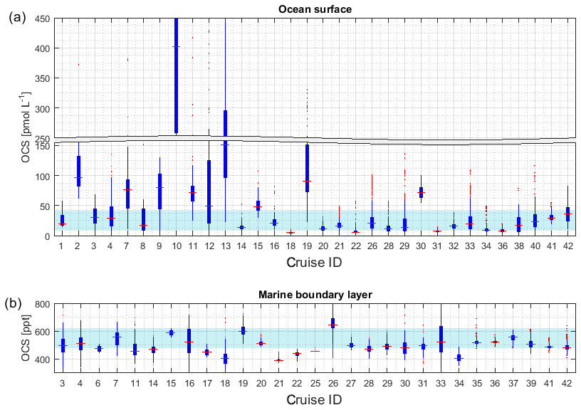
Figure 4Boxplots of measured OCS concentrations in (a) seawater and (b) marine boundary layer. Marked in red is the median of each individual dataset, the edges of the box represent the 25th and 75th percentile, and outliers are indicated by red dots. The patch in the background indicates the 20th and 80th percentile of the whole dataset. Note the break in the y axis in (a).
3.2 Carbonyl sulfide in the marine boundary layer
The dataset of OCS in the marine boundary layer includes 14 291 measurements from 30 cruises (Fig. 3f, Table 3). The average mixing ratio in the marine boundary layer is 548.9 (209–1112) ppt. All major ocean basins were covered, except for the Arctic Ocean. The North Atlantic Ocean, including the North Sea, was sampled most frequently.
Sampling of OCS in the marine boundary layer is done either discretely by pumping air in canisters, or continuously by pumping air directly into the detection system (see Table 2 for details). Marine boundary layer air was often sampled from the ship's uppermost deck, and reported sampling heights ranged from 10–35 m (Table 3). Given the relatively stable atmospheric mixing ratios (compared to the strong diel variations in dissolved OCS), a strong gradient in mixing ratios towards the sea surface is not expected. Hence, the database is suited to calculate the concentration gradient across the air–sea boundary, making it valuable for calculating oceanic emissions. The sampling frequency in individual datasets ranged from intervals shorter than hourly to monthly time series (Fig. 3f). Given the weak diurnal variability compared to the seasonal variability, the reported resolution in all of the individual datasets is sufficient for large-scale comparisons. The global variability of boundary layer OCS mixing ratio is less pronounced and does not show the same spatial pattern as that of dissolved OCS in the surface ocean (Fig. 2b). Ranges of mixing ratios are similar across all latitude bins, with minor variations (Fig. 3b). In several individual datasets, e.g., in the Pacific (Weiss et al., 1995b) and Atlantic transects (Xu et al., 2001), mixing ratios in the tropics increase compared to higher latitudes during the respective cruise (Fig. 2b). The highest atmospheric mixing ratios are reported from around Europe (including the Mediterranean), as well as off the Falkland Islands (Fig. 2b). The complete database includes measurements from January to December in the Northern Hemisphere, but data for September are missing in the Southern Hemisphere. The seasonal variability in atmospheric mixing ratio was less pronounced compared to the variability in seawater OCS concentration, with monthly medians ranging from 439–647 ppt in the Northern Hemisphere and 467–523 ppt in the Southern Hemisphere. No clear seasonal pattern was observed in either of the hemispheric datasets. The lack of such a pattern in atmospheric concentrations might result from the limited size of the dataset and the spatial heterogeneity of the sampling locations (i.e., influence of local vegetation sinks or anthropogenic sources of the air mass history). It should also be noted that small decadal trends as reported in the introduction could influence the reported differences, as the measurements reported here span a period of 1982–2018. Also, possible standardization and calibration issues could potentially be larger than the range of reported trends, so using the dataset in new trend studies should only be done with caution.
The internal consistency of the database is of similar quality as that described for OCS in seawater. A total of 60 % of the data (i.e., between 20 and 80 percentile) fall in a narrow range of 477–621 ppt (Fig. 4b). Some features are present across different datasets and thus support the internal consistency of the dataset: for example, locally elevated mixing ratios in tropical latitudes are present in single datasets and also globally (Figs. 2b and 4b). Elevated atmospheric mixing ratios were reported by several studies providing measurement from around Europe (Figs. 2b and 4b).
3.3 Carbon disulfide in seawater
Measurements of dissolved CS2 in seawater are reported from 11 cruises (Fig. 1, 1813 measurements), with an average of 15.7 (1.1–376) pmol L−1. Most of the measurements were performed in the Atlantic Ocean, comprised of three Atlantic meridional transects (Fig. 2c). No measurements are available from the Arctic and Antarctic waters and the Indian Ocean.
The latitudinal variation in CS2 in seawater was small (Fig. 5a, on average <5 pmol L−1), although individual studies report a general covariation in concentrations and water temperature (Xie and Moore, 1999; Lennartz et al., 2017). Apart from an Atlantic transect with exceptionally high concentrations (Lennartz et al., 2017), concentrations tend to increase towards coastal and upwelling regions (Fig. 2c), but this increase was less pronounced compared to the spatial variability of OCS (Fig. 2a). Seasonal variability of CS2 water concentrations was larger compared to the spatial variability (Fig. 5a and c) but did not show a clear seasonal or spatial pattern. Concentrations were comparable in the Northern Hemisphere and Southern Hemisphere. Diurnal variability of surface concentrations was present on some but not all days within individual datasets, likely representing the varying efficiency of the local sink process in the mixed layer. The occurrence of diel cycles calls for a similarly high sampling frequency to that suggested for OCS (i.e., more frequently than 4 hourly). However, most of the dataset comprises a sampling frequency of daily to monthly, and the sampling is biased towards daytime (Fig. 5e). Hence, averaged concentrations might slightly overestimate diel averages.
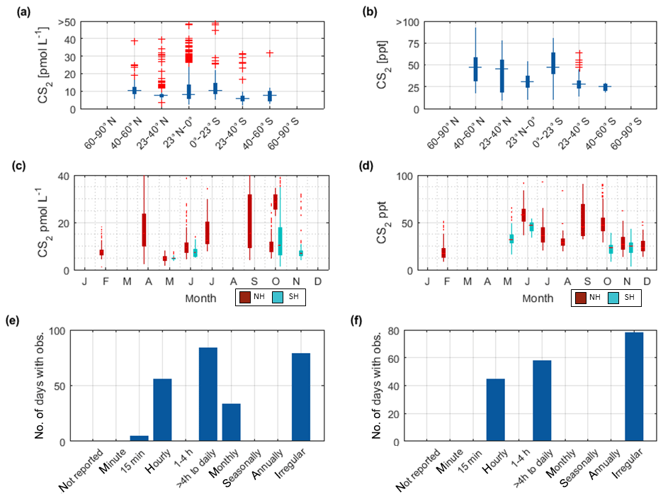
The database presented here indicates the common range of seawater concentrations and covers several biogeochemical regimes. However, limitations remain, viz., (1) a general sparsity of measurements; (2) data gaps, especially in high latitudes; and (3) insufficient sampling frequency to cover full diel variability in many individual datasets.
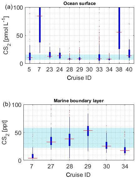
The limited size of the database for CS2 in seawater hampers internal data comparison. The majority of the data (between 20 and 80 percentile) falls in the range of 6.1–15.6 pmol L−1. Individual datasets from the Southern Ocean (cruiseID 7, not georeferenced) and from an Atlantic transect (cruiseID 38) show mean concentrations that are considerably higher than observed on other cruises (Fig. 6a). Since data from dataset ID7 represent the only available measurements for this location, based on this database, we cannot determine whether this is an artifact or not. However, we see a similar trend in the OCS data observed by dataset ID7. Also, the low atmospheric mixing ratio measured during this specific cruise speaks against a contamination problem. For the Atlantic transect it is evident that the average concentration is higher compared to the other three Atlantic cruises with a similar cruise track, i.e., dataset ID28, ID29, and ID33. However, the minimum measured concentration in this specific dataset is 7 pmol L−1, which makes a strong contamination unlikely. The atmospheric mixing ratios during cruise ID38 are also lower than those during the other two Atlantic transects, which negates a strong contamination problem. Furthermore, the covariance with temperature is evident in this and in other datasets (Xie and Moore, 1999; Lennartz et al., 2017). CS2 concentration in dataset ID38 is reported twice daily, once at 08:00–10:00 and once at 15:00–18:00 local time. Potentially, the average is misleading in this respect because it masks potential diel cycles. Daily maxima of cruise ID38 agree with daily maxima of some parts of the other Atlantic transects (ID28, 29, 33) but not on the majority of days. The minimum values over large parts of the cruise ID38 were higher than those in the cruises ID28, 29, and 33. Potentially, the minima might have been missed by the coarse sampling.
3.4 Carbon disulfide in the marine boundary layer
CS2 measurements in the marine boundary layer are only available for the Atlantic Ocean from six cruises, i.e., 1036 individual measurements. Atmospheric mixing ratios were on average 42.2 ppt (2.5 to 275.7 ppt, Fig. 2d).
The reported CS2 concentrations are generally higher than those reported from airborne measurements in previous studies, where values <10 ppt in the boundary layer have been reported (Cooper and Saltzman, 1993). An influence of continental air carrying a higher concentration of CS2 might be a possible explanation for elevated values (see, e.g., compilation in Khan et al., 2017 of up to 1200 ppt). The short atmospheric lifetime of CS2 sets a limit on long-range transport, so this explanation would only hold for coastal and shelf regions. The data reported here have undergone calibration procedures as reported in the original papers, and elevated values are consistent across different labs and locations, so the contamination problems of the local measurement systems are unlikely but cannot be ruled out completely as being responsible for the elevated mixing ratios.
Since this dataset is only comprised of four individual cruises, any perceived pattern in global variation should be taken with caution, as it might instead reflect natural variability or differences between individual laboratories. Spatiotemporal variability will become clearer once more data are available. Almost no preference is given to new measurement locations or times, as any new dataset will help to further constrain spatial and temporal variability of CS2 concentration. Latitudinal median mixing ratios varied between studies by a factor of 2, but due to the limited size of the dataset, it is currently unclear if this variation is meaningful. However, a CS2 mixing ratio of 42.2 ppt in the marine boundary layer may become relevant for calculation of oceanic emissions. Commonly, marine boundary layer concentrations of CS2 are assumed to be 0 due to its short lifetime, which will lead to an overestimation of emissions in cases where the true mixing ratio is higher, as our database indicates (at a temperature of 20 ∘C, a salinity of 35 psu, a wind speed of 7 m s−1, and a CS2 water concentration of 16 pmol L−1, the difference between 0 and 42 ppt CS2 in air leads to an overestimation of 21 %).
Due to the sparsity of data and the expected strong variability resulting from the short atmospheric lifetime, we will not use this limited dataset here for assessing the internal consistency across locations. The variation between the two Atlantic transect datasets ID28 and ID29, with a strong overlap in measured mixing ratios, seems reasonable (Fig. 6b), but more data are needed to establish a comparison on larger scale.
The data are available from the PANGEA database https://doi.org/10.1594/PANGAEA.905430 (Lennartz et al., 2019).
The full potential of an oceanic OCS and CS2 database can be exploited if measured concentrations are stored together with relevant metadata. As a minimal requirement, we recommend to report (i) the exact date of each measurement (including time of the day) and (ii) the exact location (including latitude, longitude and sample depth). This is especially important due to the photochemical production of both gases, as concentration in seawater varies strongly on diurnal and seasonal scales. To obtain a full diurnal cycle, we recommend measuring at a 4 h resolution at least to minimize errors when interpolating and averaging over the period of 1 d. Of secondary importance are physical parameters such as temperature, radiation, and wind speed. When modeling marine concentrations of OCS and CS2, it is helpful to have access to the CDOM absorbance data at a wavelength of 350 nm because parameterizations for production rates are based on this value (von Hobe et al., 2003; Lennartz et al., 2017). In order to decipher the history of the air mass and identify potential continental influence, it would also be helpful to measure additional trace gases such as CO or other anthropogenic tracers simultaneously.
In order enable the identification of large-scale patterns and the quantification of the oceanic source strength, we identify locations for future measurements. For OCS seawater concentration, large gaps exist in the open Pacific Ocean and the Arctic Ocean. The Arctic Ocean would be especially interesting due to the unique composition of dissolved organic matter derived from river input, which could influence OCS production in the water. Marine boundary layer OCS is required, especially from the Arctic Ocean. The data coverage for CS2 is very scarce, and measurements in water and marine boundary layer from high latitudes (Southern Ocean and Arctic Ocean), as well as Indian Ocean and Southern Pacific, would be especially helpful. Generally, for both gases, water concentration profiles would be helpful to understand their processes in the subsurface. This is important for CS2, which has a long lifetime in water, so that mixing processes could bring subsurface CS2 in contact with the atmosphere. Similarly, repeated measurements from the same locations would be helpful to decipher any trends.
STL and CAM started the initiative for data compilation and long-term storage. All coauthors contributed data from one or more expeditions. STL wrote the manuscript with input from all coauthors.
The authors declare that they have no conflict of interest.
We thank all captains and crew members of all cruises that are included in this database for their support in the data collection.
This research has been supported by the BMBF (ROMIC-THREAT; grant nos. BMBF-FK01LG1217A and 01LG1217B) and the Helmholtz-Association (TRASE-EC; grant no. VH-NG-819).
This paper was edited by Jens Klump and reviewed by Roisin Commane and one anonymous referee.
Aranami, K.: Seasonal and regional comparison of oceanic and atmospheric dimethylsulfide in the northern north Pacific: Dilution effects on its concentration during winter, J. Geophys. Res., 109, D12303, https://doi.org/10.1029/2003jd004288, 2004.
Belviso, S., Mihalopoulos, N., and Nguyen, B. C.: The supersaturation of carbonyl sulfide (OCS) in rain waters, Atmos. Environ.,, 21, 1363–1367, 1987.
Berkelhammer, M., Steen-Larsen, H. C., Cosgrove, A., Peters, A., Johnson, R., Hayden, M., and Montzka, S. A.: Radiation and atmospheric circulation controls on carbonyl sulfide concentrations in the marine boundary layer, J. Geophys. Res.-Atmos., 121, 13–113, 2016.
Brühl, C., Lelieveld, J., Crutzen, P. J., and Tost, H.: The role of carbonyl sulphide as a source of stratospheric sulphate aerosol and its impact on climate, Atmos. Chem. Phys., 12, 1239–1253, https://doi.org/10.5194/acp-12-1239-2012, 2012.
Chin, M. and Davis, D. D.: Global sources and sinks of OCS and CS2 and their distributions, Global Biogeochem. Cy., 7, 321–337, https://doi.org/10.1029/93gb00568, 1993.
Cooper, D. J. and Saltzman, E. S.: Measurements of atmospheric dimethylsulfide, hydrogen sulfide, and carbon disulfide during GTE/CITE 3, J. Geophys. Res.-Atmos., 98, 23397–23409, 1993.
Crutzen, P. J.: The possible importance of cso for the sulfate layer of the stratosphere, Geophys. Res. Lett., 3, 73–76, https://doi.org/10.1029/GL003i002p00073, 1976.
Cutter, G. A. and Radford-Knoery, J.: Carbonyl sulfide in two estuaries and shelf waters of the western north atlantic ocean, Mar. Chem., 43, 225–233, https://doi.org/10.1016/0304-4203(93)90228-G, 1993.
Cutter, G. A., Cutter, L. S., and Filippino, K. C.: Sources and cycling of carbonyl sulfide in the sargasso sea, Limnol. Oceanogr., 49, 555–565, 2004.
de Gouw, J. A., Warneke, C., Montzka, S. A., Holloway, J. S., Parrish, D. D., Fehsenfeld, F. C., Atlas, E. L., Weber, R. J., and Flocke, F. M.: Carbonyl sulfide as an inverse tracer for biogenic organic carbon in gas and aerosol phases, Geophys. Res. Lett., 36, L05804, https://doi.org/10.1029/2008GL036910, 2009.
Elliott, S., Lu, E., and Rowland, F. S.: Rates and mechanisms for the hydrolysis of carbonyl sulfide in natural waters, Environ. Sci. Technol., 23, 458–461, https://doi.org/10.1021/es00181a011, 1989.
Ferek, R. J. and Andreae, M. O.: The supersaturation of carbonyl sulfide in surface waters of the Pacific oceans off Peru, Geophys. Res. Lett., 10, 393–395, 1983.
Ferek, R. J. and Andreae, M. O.: Photochemical production of carbonyl sulphide in marine surface waters, Letters to Nature, 1984, 148–150, 1984.
Fischer, T., Kock, A., Arévalo-Martínez, D. L., Dengler, M., Brandt, P., and Bange, H. W.: Gas exchange estimates in the Peruvian upwelling regime biased by multi-day near-surface stratification, Biogeosciences, 16, 2307–2328, https://doi.org/10.5194/bg-16-2307-2019, 2019.
Inomata, Y., Matsunaga, K., Murai, Y., Osada, K., and Iwasaka, Y.: Simultaneous measurement of volatile sulfur compounds using ascorbic acid for oxidant removal and gas chromatography–flame photometric detection, J. Chromatogr. A, 864, 111–119, 1999.
Inomata, Y., Hayashi, M., Osada, K., and Iwasaka, Y.: Spatial distributions of volatile sulfur compounds in surface seawater and overlying atmosphere in the northwestern Pacific Ocean, Eastern Indian Ocean, and Southern Ocean, Global Biogeochem. Cy., 20, GB2022, https://doi.org/10.1029/2005gb002518, 2006.
Johnson, J. E.: Role of the oceans in the atmospheric cycle of carbonyl sulfide, PhD thesis, 1985.
Johnson, J. E. and Harrison, H.: Carbonyl sulfide concentrations in the surface waters and above the Pacific Ocean, J. Geophys. Res., 91, 7883–7888, 1986.
Kamyshny, A., Goifman, A., Rizkov, D., and Lev, O.: Formation of carbonyl sulfide by the reaction of carbon monoxide and inorganic polysulfides, Environ. Sci. Technol., 37, 1865–1872, https://doi.org/10.1021/es0201911, 2003.
Kettle, A. J., Rhee, T. S., von Hobe, M., Poulton, A., Aiken, J., and Andreae, M. O.: Assessing the flux of different volatile sulfur gases from the ocean to the atmosphere, J. Geophys. Res.-Atmos., 106, 12193–12209, https://doi.org/10.1029/2000jd900630, 2001.
Khan, A., Razis, B., Gillespie, S., Percival, C., and Shallcross, D.: Global analysis of carbon disulfide (CS2) using the 3-d chemistry transport model stochem, Aims Environmental Science, 4, 484–501, 2017.
Kim, K. H. and Andreae, M.: Carbon disulfide in seawater and the marine atmosphere over the North Atlantic, J. Geophys. Res.-Atmos., 92, 14733–14738, 1987.
Kim, K. H. and Andreae, M. O.: Carbon disulfide in the estuarine, coastal and oceanic environments, Mar. Chem., 40, 179–197, 1992.
Kremser, S., Jones, N. B., Palm, M., Lejeune, B., Wang, Y., Smale, D., and Deutscher, N. M.: Positive trends in southern hemisphere carbonyl sulfide, Geophys. Res. Lett., 42, 9473–9480, https://doi.org/10.1002/2015gl065879, 2015.
Kremser, S., Thomason, L. W., von Hobe, M., Hermann, M., Deshler, T., Timmreck, C., Toohey, M., Stenke, A., Schwarz, J. P., Weigel, R., Fueglistaler, S., Prata, F. J., Vernier, J.-P., Schlager, H., Barnes, J. E., Antuña-Marrero, J.-C., Fairlie, D., Palm, M., Mahieu, E., Notholt, J., Rex, M., Bingen, C., Vanhellemont, F., Bourassa, A., Plane, J. M. C., Klocke, D., Carn, S. A., Clarisse, L., Trickl, T., Neely, R., James, A. D., Rieger, L., Wilson, J. C., and Meland, B.: Stratospheric aerosol–observations, processes, and impact on climate, Rev. Geophys., 54, 278–335, https://doi.org/10.1002/2015rg000511, 2016.
Launois, T., Belviso, S., Bopp, L., Fichot, C. G., and Peylin, P.: A new model for the global biogeochemical cycle of carbonyl sulfide – Part 1: Assessment of direct marine emissions with an oceanic general circulation and biogeochemistry model, Atmos. Chem. Phys., 15, 2295–2312, https://doi.org/10.5194/acp-15-2295-2015, 2015.
Lennartz, S. T., Marandino, C. A., von Hobe, M., Cortes, P., Quack, B., Simo, R., Booge, D., Pozzer, A., Steinhoff, T., Arevalo-Martinez, D. L., Kloss, C., Bracher, A., Röttgers, R., Atlas, E., and Krüger, K.: Direct oceanic emissions unlikely to account for the missing source of atmospheric carbonyl sulfide, Atmos. Chem. Phys., 17, 385–402, https://doi.org/10.5194/acp-17-385-2017, 2017.
Lennartz, S. T., Marandino, C. A., von Hobe, M., Andreae, M. O., Aranami, K., Atlas, E. L., Berkelhammer, M., Bingemer, H., Booge, D., Cutter, G. A., Cortes, P., Kremser, S., Law, C. S., Marriner, A., Simo, R., Quack, B., Uher, G., Xie, H., and Xu, X.: A database for carbonyl sulfide (OCS) and carbon disulfide (CS2) in seawater and marine boundary layer, PANGAEA, https://doi.pangaea.de/10.1594/PANGAEA.905430, 2019.
Mihalopoulos, N., Putaud, J. P., Nguyen, B. C., and Belviso, S.: Annual variation of atmospheric carbonyl sulfide in the marine atmosphere in the Southern Indian Ocean, J. Atmos. Chem., 13, 73–82, https://doi.org/10.1007/bf00048101, 1991.
Mihalopoulos, N., Nguyen, B. C., Putaud, J. P., and Belviso, S.: The oceanic source of carbonyl sulfide (COS), Atmos. Environ., 26A, 1383–1394, 1992.
Montzka, S.: Noaa whole air sampler mass spectrometer analysis., Version 1.0. Ucar/ncar – earth observing laboratory, Global Monitoring Division (GMD), Earth System Research Laboratory, 2013.
Montzka, S. A.: A 350-year atmospheric history for carbonyl sulfide inferred from Antarctic firn air and air trapped in ice, J. Geophys. Res., 109, D22302, https://doi.org/10.1029/2004jd004686, 2004.
Montzka, S. A., Aydin, M., Battle, M., Butler, J. H., Saltzman, E. S., Hall, B. D., Clarke, A. D., Mondeel, D., and Elkins, J. W.: A 350‐year atmospheric history for carbonyl sulfide inferred from Antarctic firn air and air trapped in ice, J. Geophys. Res.-Atmos., 109, D22302, https://doi.org/10.1029/2004JD004686, 2004.
Montzka, S. A., Calvert, P., Hall, B. D., Elkins, J. W., Conway, T. J., Tans, P. P., and Sweeney, C.: On the global distribution, seasonality, and budget of atmospheric carbonyl sulfide (COS) and some similarities to CO2, J. Geophys. Res., 112, D09302, https://doi.org/10.1029/2006jd007665, 2007.
Moore, R. and Webb, M.: The relationship between methyl bromide and chlorophyll α in high latitude ocean waters, Geophys. Res. Lett., 23, 2951–2954, 1996.
Radford-Knoery, J. and Cutter, G. A.: Biogeochemistry of dissolved hydrogen sulfide species and carbonyl sulfide in the western North Atlantic ocean, Geochim. Cosmochim. Ac., 58, 5421–5431, https://doi.org/10.1016/0016-7037(94)90239-9, 1994.
Staubes, R. and Georgii, H.-W.: Biogenic sulfur compounds in seawater and the atmosphere of the antarctic region, Tellus, 45B, 127–137, 1993.
Staubes, R., Georgii, H. W., and Ockelmann, G.: Flux of COS, DMS and CS2 from various soils in germany, Tellus B, 41, 305–313, 1989.
Staubes, R., Georgii, H.-W., and Bürgermeister, S.: Biogenic sulfur compounds in seawater and the marine atmosphere, in: Physico-chemical behaviour of atmospheric pollutants, Springer, 686–692, 1990.
Uher, G.: Photochemische Produktion von Carbonylsulfid im Oberflächenwasser der Ozeane: Prozeßstudien und ein empirisches Modell, Universität Mainz, 147 pp., 1994.
Uher, G. and Andreae, M. O.: Photochemical production of carbonyl sulfide in North Sea water: A process study, Limnol. Oceanogr., 42, 432–442, 1997.
Ulshöfer, V. S. and Andreae, M. O.: Carbonyl sulfide (COS) in the surface ocean and the atmospheric COS budget, Atmos. Geochem., 3, 283–303, 1998.
Ulshöfer, V. S., Uher, G., and Andreae, M. O.: Evidence for a winter sink of atmospheric carbonyl sulfide in the Northeast Atlantic Ocean, Geophys. Res. Lett., 22, 2601–2604, 1995.
Ulshöfer, V. S., Flöck, O. R., Uher, G., and Andreae, M. O.: Photochemical production and air-sea exchange of carbonyl sulfide in the Eastern Mediterranean sea, Mar. Chem., 53, 25–39, 1996.
Von Hobe, M., Kettle, A. J., and Andreae, M. O.: Carbonyl sulphide in and over seawater: Summer data from the Northeast Atlantic Ocean, Atmos. Environ., 33, 3503–3514, 1999.
von Hobe, M., Kenntner, T., Helleis, F. H., Sandoval-Soto, L., and Andreae, M. O.: Cryogenic trapping of carbonyl sulfide without using expendable cryogens, Anal. Chem., 72, 5513–5515, 2000.
Von Hobe, M., Cutter, G. A., Kettle, A. J., and Andreae, M. O.: Dark production: A significant source of oceanic COS, J. Geophys. Res., 106, 31217, https://doi.org/10.1029/2000jc000567, 2001.
von Hobe, M., Najjar, R. G., Kettle, A. J., and Andreae, M. O.: Photochemical and physical modeling of carbonyl sulfide in the ocean, J. Geophys. Res., 108, 3229, https://doi.org/10.1029/2000jc000712, 2003.
Von Hobe, M., Kuhn, U., Van Diest, H., Sandoval-Soto, L., Kenntner, T., Helleis, F., Yonemura, S., Andreae, M. O., and Kesselmeier, J.: Automated in situ analysis of volatile sulfur gases using a sulfur gas analyser (SUGAR) based on cryogenic trapping and gas-chromatographic separation, Int. J. Environ. An. Ch., 88, 303–315, https://doi.org/10.1080/03067310701642081, 2008.
Watts, S. F.: The mass budgets of carbonyl sulfide, dimethyl sulfide, carbon disulfide and hydrogen sulfide, Atmos. Environ., 34, 761–779, https://doi.org/10.1016/s1352-2310(99)00342-8, 2000.
Weiss, P. S., Andrews, S. S., Johnson, J. E., and Zafiriou, O. C.: Photoproduction of carbonyl sulfide in South Pacific Ocean waters as a function of irradiation wavelength, Geophys. Res. Lett., 22, 215–218, 1995a.
Weiss, P. S., Johnson, J. E., Gammon, R. H., and Bates, T. S.: Reevaluation of the open ocean source of carbonyl sulfide to the atmosphere, J. Geophys. Res., 100, 23083–23092, 1995b.
Whelan, M. E., Lennartz, S. T., Gimeno, T. E., Wehr, R., Wohlfahrt, G., Wang, Y., Kooijmans, L. M. J., Hilton, T. W., Belviso, S., Peylin, P., Commane, R., Sun, W., Chen, H., Kuai, L., Mammarella, I., Maseyk, K., Berkelhammer, M., Li, K.-F., Yakir, D., Zumkehr, A., Katayama, Y., Ogée, J., Spielmann, F. M., Kitz, F., Rastogi, B., Kesselmeier, J., Marshall, J., Erkkilä, K.-M., Wingate, L., Meredith, L. K., He, W., Bunk, R., Launois, T., Vesala, T., Schmidt, J. A., Fichot, C. G., Seibt, U., Saleska, S., Saltzman, E. S., Montzka, S. A., Berry, J. A., and Campbell, J. E.: Reviews and syntheses: Carbonyl sulfide as a multi-scale tracer for carbon and water cycles, Biogeosciences, 15, 3625–3657, https://doi.org/10.5194/bg-15-3625-2018, 2018.
Wofsy, S. C., Afshar, S., Allen, H. M., Apel, E., Asher, E. C., Barletta, B., Bent, J., Bian, H., Biggs, B. C., Blake, D. R., Blake, N., Bourgeois, I., Brock, C. A., Brune, W. H., Budney, J. W., Bui, T. P., Butler, A., Campuzano-Jost, P., Chang, C. S., Chin, M., Commane, R., Correa, G., Crounse, J. D., Cullis, P. D., Daube, B. C., Day, D. A., Dean-Day, J. M., Dibb, J. E., Digangi, J. P., Diskin, G. S., Dollner, M., Elkins, J. W., Erdesz, F., Fiore, A. M., Flynn, C. M., Froyd, K., Gesler, D. W., Hall, S. R., Hanisco, T. F., Hannun, R. A., Hills, A. J., Hintsa, E. J., Hoffman, A., Hornbrook, R. S., Huey, L. G., Hughes, S., Jimenez, J. L., Johnson, B. J., Katich, J. M., Keeling, R., Kim, M. J., Kupc, A., Lait, L. R., Lamarque, J. F., Liu, J., McKain, K., McLaughlin, R. J., Meinardi, S., Miller, D. O., Montzka, S. A., Moore, F. L., Morgan, E. J., Murphy, D. M., Murray, L. T., Nault, B. A., Neuman, J. A., Newman, P. A., Nicely, J. M., Pan, X., Paplawsky, W., Peischl, J., Prather, M. J., Price, D. J., Ray, E., Reeves, J. M., Richardson, M., Rollins, A. W., Rosenlof, K. H., Ryerson, T. B., Scheuer, E., Schill, G. P., Schroder, J. C., Schwarz, J. P., St.Clair, J. M., Steenrod, S. D., Stephens, B. B., Strode, S. A., Sweeney, C., Tanner, D., Teng, A. P., Thames, A. B., Thompson, C. R., Ullmann, K., Veres, P. R., Vizenor, N., Wagner, N. L., Watt, A., Weber, R., Weinzierl, B., Wennberg, P., Williamson, C. J., Wilson, J. C., Wolfe, G. M., Woods, C. T., and Zeng, L. H.: Atom: Merged atmospheric chemistry, trace gases, and aerosols, ORNL Distributed Active Archive Center, ORNL DAAC, Oak Ridge, Tennessee, USA, https://doi.org/10.3334/ORNLDAAC/1581, 2018.
Xie, H. and Moore, R. M.: Carbon disulfide in the North Atlantic and Pacific Oceans, J. Geophys. Res., 104, 5393, https://doi.org/10.1029/1998jc900074, 1999.
Xu, X., Bingemer, H. G., Georgii, H. W., Schmidt, U., and Bartell, U.: Measurements of carbonyl sulfide (cos) in surface seawater and marine air, and estimates of the air-sea flux from observations during two Atlantic cruises, J. Geophys. Res., 106, 3491, https://doi.org/10.1029/2000jd900571, 2001.
Zhang, L., Walsh, R. S., and Cutter, G. A.: Estuarine cycling of carbonyl sulfide: Production and sea-air flux, Mar. Chem., 61, 127–142, 1998.