A cultivated planet in 2010 – Part 2: The global gridded agricultural-production maps

Data on global agricultural production are usually available as statistics at administrative units, which does not give any diversity and spatial patterns; thus they are less informative for subsequent spatially explicit agricultural and environmental analyses. In the second part of the two-paper series, we introduce SPAM2010 – the latest global spatially explicit datasets on agricultural production circa 2010 – and elaborate on the improvement of the SPAM (Spatial Production Allocation Model) dataset family since 2000. SPAM2010 adds further methodological and data enhancements to the available crop downscaling modeling, which mainly include the update of base year, the extension of crop list, and the expansion of subnational administrative-unit coverage. Specifically, it not only applies the latest global synergy cropland layer (see Lu et al., submitted to the current journal) and other relevant data but also expands the estimates of crop area, yield, and production from 20 to 42 major crops under four farming systems across a global 5 arcmin grid. All the SPAM maps are freely available at the MapSPAM website (http://mapspam.info/, last access: 11 December 2020), which not only acts as a tool for validating and improving the performance of the SPAM maps by collecting feedback from users but is also a platform providing archived global agricultural-production maps for better targeting the Sustainable Development Goals. In particular, SPAM2010 can be downloaded via an open-data repository (DOI: https://doi.org/10.7910/DVN/PRFF8V; IFPRI, 2019).

1 Introduction

Civilization is founded on the agricultural use of land (Fu and Liu, 2019), which remains as important today as it was 10 000 years ago (Lev-Yadun et al., 2000). Agricultural land, which refers to the land area that is arable, under permanent crops, and under permanent meadows and pastures according to the Food and Agriculture Organization of United Nations (FAO), is currently 4.9 billion ha in 2019. This is 37.6 % of the earth's terrestrial surface – the largest use of land on the planet. Historically, the agricultural use of land has transformed ecosystem patterns and processes across most of the terrestrial biosphere (Ellis et al., 2013). The way we use agricultural land will significantly determine whether we are able to solve the multiple challenges embodied in the 17 Sustainable Development Goals (SDGs), e.g., feeding the world's growing population, mitigating climate change, and halting biodiversity loss (FAO, 2018; Ehrensperger et al., 2019). As the fundamental connection between people and the planet, the spatiotemporal characteristics of agricultural land is important for the anthroposphere and beyond as such information allows us to undertake more responsive and evidence-based analysis on the interaction and better resource allocation across land, water, energy, and the environment.

Cropland mapping has made great progress in the past few decades and provided great support for global agricultural monitoring and assessment. For example, it allows us to be able to know where agriculture has infringed into natural ecosystems and where cropland has been taken as a consequence of urbanization (Chen et al., 2015; Gong et al., 2019). However, this type of work mainly focuses on the agricultural changes at the land cover level, without paying attention to the subtle characteristics at the land use and land management level (Verburg et al., 2011). These subtle level characteristics related to agricultural production, ranging from crop allocation to land use intensity, are the core of agricultural management and have been proven to have equally important impacts on food systems (Sun et al., 2018; Pretty, 2018), climate systems (Searchinger et al., 2018; Bonan and Doney, 2018), and ecosystems (Peters et al., 2019; Poore and Nemecek, 2018). Yet data on global agricultural production are usually representative at national and subnational administrative units (e.g., provinces, districts). This level of statistics does not give a sense of the diversity and spatial patterns in agricultural production and is not spatially explicit, which is critical for many environmental and ecological assessments (Yu et al., 2012).

There are a few attempts to develop global spatially explicit datasets on agricultural production by fusing census statistics with maps of agricultural land cover (Fig. 1). Leff et al. (2004) applied a simplified proportional disaggregating approach and mapped the global harvested area of 18 major crops circa 1992. By using a similar approach, Monfreda et al. (2008) mapped both harvested area and yield for a full coverage of 175 crops circa 2000 (the dataset is referred to as M3 hereafter). Portmann et al. (2010) developed the MIRCA (Monthly Irrigated and Rainfed Crop Areas) dataset that contains the harvested area for 26 crops circa 2000 by using M3 as a starting point. It further allocates the total harvested area for each crop into rainfed and irrigated areas. Fischer et al. (2012) developed the GAEZ dataset (Global Agro-ecological Zones), which contains the potential harvested area and yield for 23 crops circa 2000 considering the crop-specific agroclimatic and edaphic suitability criteria. You and Wood (2006) developed the Spatial Production Allocation Model (SPAM) firstly at the continental scale then subsequently at the global scale by using an entropy-based model to downscale crop production. The first global SPAM dataset is available for the year 2000, at the time when M3, MIRCA, and GAEZ were also available (Fig. 1).

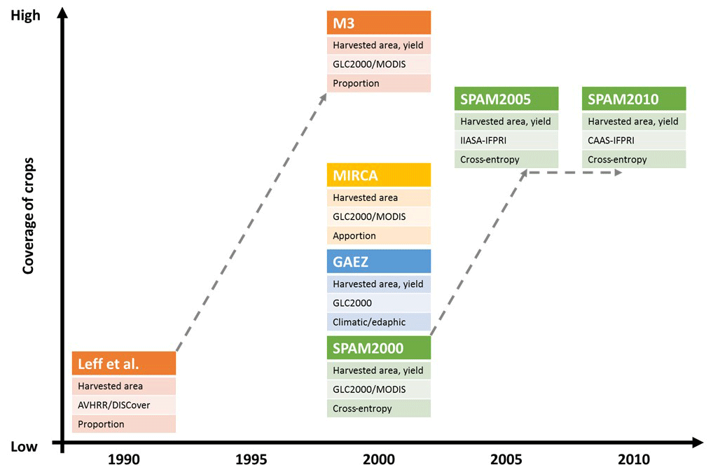
Figure 1 Overview of the global spatially explicit datasets on agricultural production. Each dataset is plotted in a coordinate system with the x axis representing the time span and the y axis representing the number of crops that have been included. For each dataset, the first row indicates the major measurement(s) of agricultural production, the second row indicates the cropland cover layer, and the third row indicates the main approach for allocating production. The dashed line within the chart indicates the evolution of a dataset family.

Changes in agricultural lands over time are as important as over space, especially given that the changes in cropping pattern and crop yields are more frequent than those at the land cover level (Verburg et al., 2011). While there are four spatially explicit datasets on global agricultural production available around the year 2000 (Anderson et al., 2015), three of them, i.e., M3, MIRCA, and GAEZ, are no longer available after 2000. Agricultural-production systems are constantly changing, and these changes are not trivial. However, a lot of recent agricultural and environmental assessments were still based on those maps produced decades ago (Deutsch et al., 2018; Nanni et al., 2019; Estes et al., 2018; Prestele et al., 2018; Erb et al., 2018; Porwollik et al., 2019; Yu et al., 2017b), suggesting that an update of existing global agricultural-production maps is very desirable for subsequent analysis.

SPAM had committed to updating maps every 5 years (You et al., 2014; Wood-Sichra et al., 2016), which substantially fills the data gap and extends the work for global agricultural-production mapping by operating a global gridscape at the confluence between earth and farming systems in multiple time stages. The SPAM model has become a critical tool to many initiatives within and beyond the Consultative Group for International Agricultural Research (CGIAR). Moreover, SPAM data are frequently downloaded and widely used by researchers and analysts from international originations, academia, and governments agencies all over the world. The global spatially explicit datasets in multiple time stages enable scientists as well as policymakers to better address the global change challenges within the anthroposphere and beyond, such as targeting agricultural and rural development policies and investments and increasing food security and growth with minimal environmental impacts. Successful examples include AGRODEP (African Growth and Development Policy Modeling Consortium) Library (http://www.agrodep.org/fr/node/1794, last access: 11 December 2020), GEOGLAM (Global Agricultural Monitoring Initiative) (http://www.geoglam.org, last access: 11 December 2020), USAID (United States Agency for International Development) Feed the Future Innovation Lab for Small-scale Irrigation (https://ilssi.tamu.edu/, last access: 11 December 2020), Africa Infrastructure (https://openknowledge.worldbank.org/handle/10986/2692, last access: 11 December 2020), and so on. In this paper, we introduce SPAM2010, the latest update of the SPAM family. The next section gives an overview of the SPAM model. Section 3 provides a detailed description and improvements of SPAM2010. Section 4 introduces the data preparation, and Sect. 5 presents some of the results produced by SPAM2010. Finally, we conclude with some advice on using the maps and our own plan for the future of SPAM.

2 SPAM overview

The main purpose of SPAM is to disaggregate crop statistics (e.g., harvested area, production quantity, and yield) by different farming systems and to further allocate such disaggregated statistics into spatially gridded units (Fig. 2). In SPAM, disaggregation is processed before allocation because crop yields are likely to be substantially different between different farming systems (e.g., irrigation versus rainfed) even at the same location. The whole procedure entails a data fusion approach that combines information from different sources and at different spatial scales by deploying various matching and calibration processes. Then all the data elements are processed by the optimization model, which generates results at the grid level (Fig. 2).

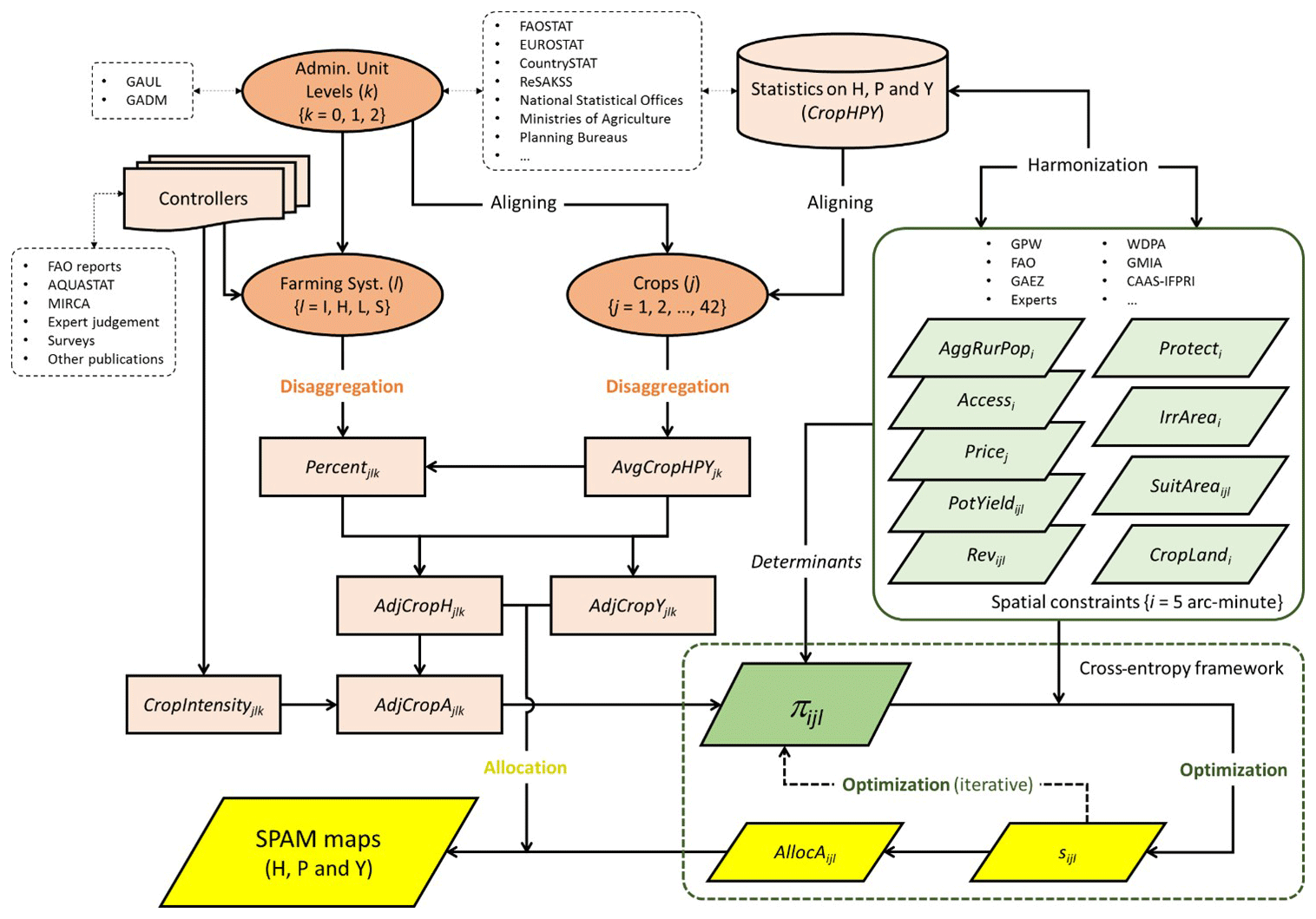
Figure 2 The overall structure of the SPAM model. The rhombuses indicate spatial data inputs and outputs, while the other shapes indicate nonspatial data inputs (see the detailed data description in the following section). The orange color indicates how crop statistics are disaggregated by administrative unit (k), crop type (j), and farming system (l). The green color indicates how the spatial parameters are collected and prepared at a unified spatial resolution (i) and in a harmonized manner. The yellow color indicates the spatial allocation inputs/outputs. The darker colors, either in orange or in green, highlight the essential elements in SPAM: the former indicates the farming system disaggregation scheme, while the latter indicates (i.e., priors of physical area) a key parameter with which the spatial and nonspatial data are connected and the iterative spatial allocation is able to take place.

The SPAM methodology was first developed in a trial project for six major crops in Latin America and the Caribbean by combining satellite imagery and crop statistics. Later on, it was used to derive regional estimates of spatially disaggregated crop production in Brazil and sub-Saharan Africa (You and Wood, 2006; You et al., 2009). Over the years the model has evolved, adding more crops and using additional data and increasingly complicated optimization equations as well as expanding to global coverage (You et al., 2014). The SPAM methodology is different from its counterparts. For example, M3 has no distinction across farming systems and is allocated proportionally (within each crop) to each grid cell within each subnational unit; hence the M3 dataset provides interpolated estimates of output by crop at the resolution of the satellite data (Fig. 1). SPAM not only considers the crop yield variation across farming systems but also assigns production weighted by price to grid cells rather than pure proportionality (Donaldson and Storeygard, 2016). Moreover, MIRCA and GAEZ focus more on the biophysical aspects of agricultural production, while SPAM uses a triangulation of any and all relevant background and partial information, which includes not only national or subnational crop production statistics and satellite data on land cover but also maps of irrigated areas, crop potential suitability, secondary data on population density, market accessibility, cropping intensity, and crop prices (Fig. 2).

The SPAM model produces global gridded maps of agricultural production at a 5 arcmin spatial resolution. The first SPAM maps, known as SPAM2000, represent global agricultural production circa 2000 for 20 crops, with the exception of a few small island states and conflict zones (You et al., 2014). Subsequently, the SPAM maps have been updated every 5 years. SPAM2005 acts as an intermediate update which expands the coverage of crops from SPAM2000. The 42 crop categories are further adopted in SPAM2010 (Fig. 1).

3 Model improvement for SPAM2010

There are three submodules in a standardized SPAM model: disaggregation, optimization, and allocation. We conceptualize the SPAM2010 based on this general setting, while it adds further methodological and data improvements, which mainly include the update of base year, the expansion of subnational administrative-unit coverage, the extension of crop list, and the substitution of the latest hybrid cropland map as the basic allocation layer. Considering the huge number of input data and multiple-year efforts, such an update is not trivial and will be critical for the user community. In this section, we briefly introduce the model structure and how these submodules are processed and connected.

3.1 Disaggregation

The first step for SPAM is to disaggregate crop statistics of agricultural production (e.g., the yield, harvested area, and total production) by administrative-unit levels (k), crop type (j), and farming system (l) from coarser scale to finer scale (illustrated by orange shapes in Fig. 2). For example, the national-level statistics are disaggregated into subnational levels, statistics for crop aggregates are divided into individual crop types, and the crop statistics are further separated by rainfed and irrigated conditions. Disaggregation is a nonspatial module. For the administrative unit (ADM), we consider three levels – k=0 (national level), 1 (subnational level 1), and 2 (subnational level 2) – and refer to the country-specific administrative level as the statistical reporting units (SRUs; SRU =k₀, k₁ or k₂). In general, the SPAM model will have better performance if crop statistics are more disaggregated by the ADM. Therefore, we prefer to collect crop statistics for ADM1 and ADM2, despite statistics mostly being available at the ADM0 level and the subnational coverage always being less complete. Comparing to the previous SPAM products, the subnational coverage percentage has increased markedly for SPAM2010, which is described in detail in Sect. 4.1.

We improve the model capacity in SPAM2010 as well: we simultaneously allocate 42 crops and crop aggregates (versus the 20 crops and crop aggregates in SPAM2000) and consider four farming systems for each crop (Fig. 2). In SPAM2010, we keep the farming systems conceptualized for SPAM2000, which have proven to be useful to represent the different crop performances under different management systems; e.g., the irrigated yields of a particular crop are likely to be substantially different from the corresponding rainfed yields. The four farming systems are defined as follows:

• The irrigated farming system (I) refers to the crop area equipped with either full or partial control irrigation. Normally the crop production on the irrigated fields uses a high level of inputs such as modern varieties and fertilizer as well as advanced management such as soil and water conservation measures.

• The rainfed high-input farming system (H) refers to the market-oriented crop area, which uses high-yield varieties; machinery with low labor intensity; and optimum applications of nutrients and chemical pest, disease, and weed control.

• The rainfed low-input farming system (L) refers to crop area which uses traditional varieties and mainly manual labor without (or with little) application of nutrients or chemicals for pest and disease control. Production is mostly for personal consumption.

• The rainfed subsistence farming system (S) is introduced to account for situations where cropland and suitable areas do not exist, but farmland is still present in some way. Production is mostly for personal consumption, which is also low-input.

The four conceptualized farming systems are mainly delineated by the water supply system and inputs used by farmers, despite global data on farming system shares for each crop being largely absent. For a small number of large countries, e.g., Brazil, China, India, Russia, the United States (see more details in Sect. 4.1), we have data on farming system shares at the ADM1 level. For the other countries we first assign the national farming system shares to each ADM1 level and then adjust individual ADM1 farming system shares in light of the supporting evidence. For example, if the national share for irrigation of wheat was 30 %, we assign that to all ADM1 units. Then we look at individual units, and if supporting evidence (e.g., the Global Map of Irrigation Areas, GMIA, data) indicates that there was no irrigated area present in a particular AMD1 unit, we set the irrigation share of wheat to 0 in that administrative unit. Finally the farming system shares at the national level are recalculated as the weighted average of the adjusted ADM1 estimates. For a few countries which have very limited data accessibility, experts may give their opinions. For example, it was often necessary to use farming system shares from one crop as proxies for similar crops (e.g., farming system shares for beans are used for all pulses) or to apply shares from one country to similar countries (e.g., the geographically smaller countries in the Middle East, including Kuwait, Oman, and Qatar, are assigned the same farming system shares).

For irrigated farming systems, the crop-specific shares are derived by dividing the harvested area cultivated under full-control irrigation obtained from AQUASTAT, MIRCA, and country-level statistics by the overall harvested area. For rainfed farming systems, crop-specific shares are primarily estimated based on generalized assumptions for individual countries and crops. For example, all cereals in western Europe are produced with high inputs, whereas 20 % of cereals in sub-Saharan Africa are grown under a subsistence farming system. We also assume fertilization as a proxy for high-input use, so if irrigated crop areas and overall fertilized and nonfertilized areas of a crop are known, it is possible to deduce rainfed–high shares by subtracting the irrigated areas from fertilized areas. The remainder of fertilized area will be then classified as rainfed–high, and the nonfertilized areas will be further split between rainfed–low and rainfed–subsistence. In addition, the shares of rainfed–subsistence are assigned when there is not enough suitable area for rainfed–low conditions to satisfy the completeness of disaggregated crop statistics in terms of area extent and/or production quantity. In such cases a portion of the rainfed–low statistics were assumed to stem from rainfed–subsistence. Although disaggregation is a nonspatial module of SPAM, it is applied interactively with the spatial modules by the support of multiple spatial data and nonspatial data, which are elaborated in detail in the section “Data preparation for SPAM2010”.

3.2 Optimization

The core part of the SPAM model is the cross-entropy module (illustrated by the dashed green frame in Fig. 2), which is used to achieve the allocation for each spatial grid (i). It works by (iteratively) minimizing the error between the preallocated shares of physical area (π_ijl) and the allocated shares of physical area (s_ijl) in each pixel i by crop j and production system l:

$$\begin{array}{}\text{(1)}& \begin{array}{rl}& \underset{\mathit{\left\{}{s}_{ijl}\mathit{\right\}}}{min}\mathrm{CE}\left(s_{ijl},{\mathit{\pi }}_{ijl}\right)={\sum }_i{\sum }_j{\sum }_l{s}_{ijl}\ln s_{ijl}\\ & -{\sum }_i{\sum }_j{\sum }_l{s}_{ijl}\ln {\mathit{\pi }}_{ijl},\end{array}\end{array}$$

where CE is the abbreviation for cross-entropy, which is defined as the log function of probability. The difference between {sln s} versus {sln π} means the estimated probability s and its prior probability π are minimized subject to certain constraints.

• i.

  Constraint specifying the range of allocated physical-area shares:

  $$\begin{array}{}\text{(2)}& \mathrm{0}\le s_{ijl}\le \mathrm{1},\forall i\forall j\forall l;\end{array}$$
• ii.

  Constraint specifying the sum of allocated physical-area shares within a grid:

  $$\begin{array}{}\text{(3)}& {\sum }_i{s}_{ijl}=\mathrm{1},\forall j\forall l;\end{array}$$
• iii.

  Constraint specifying that the sum of allocated physical area over all crops and farming systems within a grid should not exceed the actual cropland within the same grid:

  $$\begin{array}{}\text{(4)}& \begin{array}{rl}& {\sum }_j{\sum }_l{\mathrm{AdjCropA}}_{jl{k}_{\mathrm{SRU}}}\times s_{ijl}\le {\mathrm{AdjCropLand}}_i,\\ & \forall i\in k_{\mathrm{SRU}};\end{array}\end{array}$$
• iv.

  Constraint specifying that the allocated physical area by grid, crop, and farming system should not exceed the suitable area within the grid with the corresponding crop and farming system:

  $$\begin{array}{}\text{(5)}& {\mathrm{AdjCropA}}_{jl{k}_{\mathrm{SRU}}}\times s_{ijl}\le {\mathrm{AdjSuitArea}}_{ijl},\forall i\in k_{\mathrm{SRU}};\end{array}$$
• v.

  Constraint specifying that the sum of allocated physical area over all farming systems within a subnational unit should be equal to the sum of statistical physical area over all farming systems within the corresponding subnational unit:

  $$\begin{array}{}\text{(6)}& \begin{array}{rl}& {\sum }_{i\in k_{\mathrm{SRU}}}{\sum }_l{\mathrm{AdjCropA}}_{jl{k}_{\mathrm{SRU}}}\times s_{ijl}\\ & ={\sum }_l{\mathrm{AdjCropA}}_{jl{k}_{\mathrm{SRU}}},\forall j\in P,\end{array}\end{array}$$

  where P is the set of commodities for which subnational statistics exist;

• vi.

  Constraint specifying that the sum of allocated physical area under an irrigated farming system within the grid should not exceed the area equipped for irrigation in the grid:

  $$\begin{array}{}\text{(7)}& \begin{array}{rl}& {\sum }_{j\in Q}{\mathrm{AdjCropA}}_{jI{k}_{\mathrm{SRU}}}\times s_{ij\mathrm{I}}\le {\mathrm{AdjIrrArea}}_i,\\ & \forall i\in k_{\mathrm{SRU}},\end{array}\end{array}$$

  where Q is the set of commodities which are fully or partly irrigated within grid i.

Shares s_ijl are the probability values between 0 and 1:

$$\begin{array}{}\text{(8)}& s_{ijl}={\displaystyle \frac{{\mathrm{AllocA}}_{ijl}}{{\mathrm{AdjCropA}}_{jl}}},\end{array}$$

where AdjCropA_jl is the total physical area of a given SRU for crop j at input level l to be allocated. AllocA_ijl is the area allocated to grid i for crop j at input level l.

π_ijl indicates the decision to produce a particular crop under a specific production system, which is normally dependent on both biological and economic factors. However, subsistence farmers mainly grow crops for their own consumption, largely uncoupled from price, market access, or crop-potential-suitability conditions. Therefore, we first assume that the prior allocation for subsistence physical area (${\stackrel{\mathrm{‾}}{\mathrm{CropA}}}_{ij\mathrm{S}}$) in grid i by crop j under this circumstance is simply dependent on rural population density:

$$\begin{array}{}\text{(9)}& {\stackrel{\mathrm{‾}}{\mathrm{CropA}}}_{ij\mathrm{S}}={\mathrm{AdjCropA}}_{jk\mathrm{S}}\times {\displaystyle \frac{{\mathrm{AggRurPop}}_i}{{\sum }_{i\in k}{\mathrm{AggRurPop}}_i}}\forall i\forall j,\end{array}$$

where AdjCropA_jkS is the generated physical area for crop j at the subsistence farming system for the given SRU k, and AggRurPop_i is the rural population density at grid i (see the detailed description in Sect. 4).

Then for the three remaining farming systems, we assume that the potential unit revenue of planting a certain crop (Rev_ijl) would affect farmers' crop choices:

$$\begin{array}{}\text{(10)}& \begin{array}{rl}& {\mathrm{Rev}}_{ijl}={\displaystyle \frac{{\mathrm{AdjCropA}}_{jl{k}_{\mathrm{SRU}}}}{{\sum }_i{\mathrm{AdjCropland}}_i}}\times {\mathrm{Price}}_j\times {\mathrm{Access}}_i\\ & \times {\mathrm{PotYield}}_{ijl},\end{array}\end{array}$$

where AdjCropland_i, Price_j, Access_ij, and PotYield_ijl are the adjusted cropland area, market price, accessibility parameter, and potential-yield values for crop j in farming system l and grid i (see the detailed description in the following Sect. 4).

Then we assume that the priors for the remaining three farming systems are mainly influenced by the estimated revenue, cropland area, and irrigated area.

For an irrigated farming system (I),

$$\begin{array}{}\text{(11)}& {\stackrel{\mathrm{‾}}{\mathrm{CropA}}}_{ij\mathrm{I}}={\mathrm{AdjIrrArea}}_i\times {\displaystyle \frac{{\mathrm{Rev}}_{ij\mathrm{I}}}{{\sum }_j{\mathrm{Rev}}_{ij\mathrm{I}}}}\forall i\forall j.\end{array}$$

For rainfed–high (H) and/or a rainfed–low (L) farming systems,

$$\begin{array}{}\text{(12)}& \begin{array}{rl}& {\stackrel{\mathrm{‾}}{\mathrm{CropA}}}_{ijl}=\left({\mathrm{AdjCropLand}}_i-{\mathrm{AdjIrrArea}}_i-{\stackrel{\mathrm{‾}}{\mathrm{CropA}}}_{ij\mathrm{S}}\right)\\ & \times {\displaystyle \frac{{\mathrm{Rev}}_{ijl}}{{\sum }_j{\mathrm{Rev}}_{ijl}}},l=\mathrm{HL}\forall i\forall j,\end{array}\end{array}$$

where AdjCropLand_i and AdjIrrArea_i are the cropland area and irrigated area at grid i (see the detailed description in the following Sect. 4).

Finally, the main inputs for the optimization procedure are converted to shares and written as

$$\begin{array}{}\text{(13)}& {\mathit{\pi }}_{ijl}={\displaystyle \frac{{\stackrel{\mathrm{‾}}{\mathrm{CropA}}}_{ijl}}{{\sum }_{i\in k_{\mathrm{SRU}}}{\stackrel{\mathrm{‾}}{\mathrm{CropA}}}_{ijl}}}.\end{array}$$

The optimization module in SPAM2010 is almost the same as that in previous versions. We apply the cross-entropy process in the General Algebraic Modeling System (GAMS), which ensures that the optimization procedure iterates until a solution is found. Once the allocation is successful, meaning that an optimal or locally optimal solution has been found, the routine immediately returns the allocated physical area (AllocA_ijl) by grid i, crop j, and farming system l, and the program continues with postprocessing automatically (Fig. 2). If the solution is infeasible or nonoptimal, the program stops, allowing for manual scrutiny, adjustment, and rerun (see data harmonization in the following section).

3.3 Allocation

Using the results of the optimization, the allocation module produce maps of harvested area (AllocH_ijl), yield (AllocY_ijl), and production quantity (AllocP_ijl) for each grid i by crop j and farming system l (Fig. 2). For harvested area, we convert the allocated physical area (AllocA_ijl) to allocated harvested area (AllocH_ijl) by multiplying by cropping intensity (CropIntensity_jlk):

$$\begin{array}{}\text{(14)}& {\mathrm{AllocH}}_{ijl}={\mathrm{AllocA}}_{ijl}\times {\mathrm{CropIntensity}}_{jlk}.\end{array}$$

For yield, we first calculate an average potential yield (${\stackrel{\mathrm{‾}}{\mathrm{PotYield}}}_{jl{k}_{\mathrm{SRU}}}$) within an SRU using the allocated harvested area as weight, then the allocated yield (AllocY_ijl) is estimated as

$$\begin{array}{}\text{(15)}& {\mathrm{AllocY}}_{ijl}={\displaystyle \frac{{\mathrm{AdjPotYield}}_{ijl}\times {\mathrm{AdjCropY}}_{jl{k}_{\mathrm{SRU}}}}{{\stackrel{\mathrm{‾}}{\mathrm{PotYield}}}_{jl{k}_{\mathrm{SRU}}}}},\end{array}$$

where the average potential yield is calculated as

$$\begin{array}{}\text{(16)}& {\stackrel{\mathrm{‾}}{\mathrm{PotYield}}}_{jl{k}_{\mathrm{SRU}}}={\displaystyle \frac{{\sum }_{i\in \mathrm{SRU}}\left({\mathrm{AdjPotYield}}_{ijl}\times {\mathrm{AllocH}}_{ijl}\right)}{{\sum }_{i\in k_{\mathrm{SRU}}}{\mathrm{AllocH}}_{ijl}}}.\end{array}$$

We finally estimate the production quantity (AllocP_ijl) as

$$\begin{array}{}\text{(17)}& {\mathrm{AllocP}}_{ijl}={\mathrm{AllocH}}_{ijl}\times {\mathrm{AllocY}}_{ijl}.\end{array}$$

4 Data preparation for SPAM2010

The largest amount of effort to create a SPAM map is spent on identifying, collecting, and harmonizing data. For the production of SPAM2010, we collect raw data from two major sources: we first collect nonspatial crop statistics for the data disaggregation process; we then collect and/or create multiple spatially explicit constraint maps at a 5 arcmin resolution from both biophysical and socioeconomic aspects for the spatial optimization and allocation processes. Afterwards, we introduce how these multisourced data are harmonized and how data adjustment is taking place.

4.1 Crop statistics

4.1.1 Crop statistics disaggregated by administrative units

We start with the administrative units (k) for which we have been able to obtain crop production statistics (Fig. 2). We primarily used the FAO's Global Administrative Unit Layers (GAUL) at both the national and subnational levels to relate the tabulated crop statistics to gridded data during the allocation process. GAUL contains shapefiles for three administrative-level units: ADM0 (national level 0), ADM1 (subnational level 1), and ADM2 (subnational level 2). Shapefiles from the Database of Global Administrative Areas (GADM) are used for ADM1 and ADM2 in China since they proved to be easier to match to the statistics.

We collect crop statistics from FAOSTAT, EUROSTAT, CountrySTAT, ReSAKSS, national statistical offices, ministries of agriculture or planning bureaus of individual countries, household surveys, and a variety of ad hoc reports related to a particular crop within a particular country (Fig. 2). SPAM estimates are most dependent on the degree of disaggregation of the underlying national and subnational production statistics, so it is important to identify and collect as many subnational statistics as possible (Joglekar et al., 2019). Although we prefer to collect crop statistics for ADM1 and ADM2 and run the model at the ADM1 level for all countries, crop statistics are unfortunately mostly available at the ADM0 level, the subnational coverage being less complete. Therefore, for most countries we run SPAM at an ADM0 level, except for some (geographically) large countries that are modeled at an ADM1 level. We summarize the subnational data coverage by region in Table 1. We present the detailed procedure for collecting crop statistics in the Supplement (Sect. S1), which further contains a table listing all countries that are modeled at an ADM1 level (Table S1) and a table listing the sources of crop statistics by country and subnational coverage (Table S2) for all countries.

Table 1 Subnational coverage of crop production statistics by region.

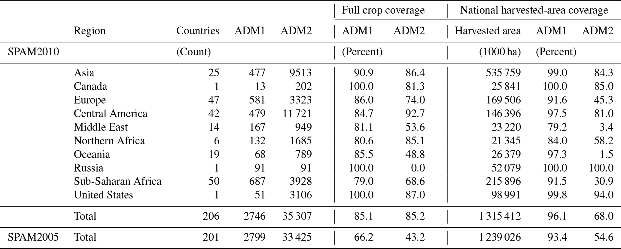
Source: assembled by authors. Note: full crop coverage refers to the percentage of crops at the administrative level with positive values or 0 in relation to all possible crops. Percent of national harvested area covered by ADM1 or ADM2 is the share of national area harvested reported by ADM1 or ADM2 units. In Russia we had no data for ADM2 units. The last row presents an overview of data coverage applied for SPAM2005 as a comparison.

We collect data in all the ADM1 units in the United States, Russia, and Canada and at least 80 % of the ADM1 units for the remaining regions worldwide, while Europe, the Middle East, Oceania, Russia, and sub-Saharan Africa have data collected on the full set of crops in below 80 % of their ADM2 units. This coverage is substantially improved for SPAM2010 in comparison to that for SPAM2005, which is only 66.2 % and 43.2 % for ADM1 and ADM2, respectively (Table 1).

Monfreda et al. (2008) reported that 81 % of the global harvested-area data in their M3 in the year 2000 came from subnational sources, but they do not distinguish coverage by subnational levels 1 and 2. SPAM often has higher levels of subnational coverage than M3, especially in Africa and the former states of the Soviet Union. This can be seen in SPAM2005; e.g., 93.4 % of global data came from ADM1 sources and 54.6 % from ADM2 sources (Wood-Sichra et al., 2016). In SPAM2010, such coverage rates are further increased to 96.1 % and 68.0 %, respectively (Table 1).

4.1.2 Crop statistics disaggregated by crop types

We simultaneously allocate 42 crops and crop aggregates (j) for SPAM2010 (Fig. 2). The crop categories are driven by the definitions of the FAO's Statistical Database (FAOSTAT). Comprised of 33 individual crops (e.g., wheat, rice, maize, barley, potato, bean, cotton) and nine crop aggregates (e.g., other cereal, vegetables), the SPAM2010 crop list covers all crops reported by the FAO, except for explicit fodder crops (mostly grasses), which are not modeled. When multiple FAO crops fall into a single SPAM2010 crop category (e.g., vegetables), the FAO's corresponding area and production data were summed up, and yields were calculated as a weighted average. We present the detailed procedure for aligning the crop types in the Supplement (Sect. S2), which further contains a full list of crops and their respective FAO code (Table S3).

We collect statistics on harvested area (H), production (P), and yield (Y; CropHPY) by each crop j in each administrative unit k for data disaggregation (Fig. 2). We prepare data for the model based on the 2009–2011 average of the crop production statistics (AvgCropHPY_jk). If data are missing from this time period, we use the average from the available data spanning the closest years between 2005 and 2015. We make corrections for discrepancies in statistical reporting units, crop names, and units of measurement during the initial cleaning phase of the data. For example, we adjust all national and subnational statistics (AdjCropHPY_jk) using the national 2009–2011 average from FAO. In order to improve the comparability of the crop production statistics across countries, we explicitly distinguish between crops not grown in an area (coded as 0) and crop data that are not available for an area (coded as a missing value). Despite the possible uncertainties in FAO data, it has been chosen as the baseline in the adjustment of country statistics mainly because (1) FAO data are the most widely acknowledged global agricultural statistics and are hence the most appropriate source for the purpose, and (2) SPAM products have been used by many global models such as IMPACT from the International Food Policy Research Institute (IFPRI; https://www.ifpri.org/project/ifpri-impact-model, last access: 11 December 2020) and GLOBIOM from the International Institute for Applied Systems Analysis; https://iiasa.ac.at/web/home/research/GLOBIOM/GLOBIOM.html, last access: 11 December 2020). These models use FAO country data for cross-country comparisons, and they need our maps to be consistent with FAO data. In fact, the idea of conceptualizing SPAM is to spatially allocate statistics from administrative units to spatial grids, and the maps could be easily adjusted to any other country data. We present the detailed procedure for adjusting the crop statistics in the Supplement (Sect. S3).

4.1.3 Crop statistics disaggregated by farming systems

We elaborated the disaggregation module for obtaining the farming system shares by crop j and administrative unit k (Percent_jlk) in Sect. 3.1. In some countries there are statistics, in others experts may give their opinions, or assumptions are made as to how some crops are grown in a similar way as other crops. Supplementing Sect. 3.1, we present more details on the procedure for obtaining the farming system shares in the Supplement (Sect. S4), which further contains a table listing the sources of subnational farming systems data (Table S4) and a table listing the farming system shares by crop groups and selected countries (Table S5). For example, shares of the irrigated farming system were taken directly for country statistics like Brazil, China, and the United States at ADM1. For some countries these figures were found in MIRCA, and yet for the rest of the countries, AQUASTAT provides information on irrigated areas per crop at the national level. We are able to source data on farming system shares at the ADM1 level for limited large countries (Table S4). Based on this list we showcase the shares of production under irrigated and rainfed systems for selected crop groups and countries (Table S5). We choose Brazil, China, Ethiopia, France, India, Indonesia, Nigeria, Turkey, and the United States because they vary in agroecology, region, income level, and geographical size. For cereal crops, the three Asian countries (China, India, and Indonesia) have the highest shares of irrigated area, whereas the two sub-Saharan countries (Ethiopia and Nigeria) have the lowest shares of irrigated area. For root, tuber, and pulse production, the United States and both European countries have the highest shares of irrigated areas, while the sub-Saharan countries again have less than 1 % each. Aggregating across all crops, the three Asian countries rank highest in terms of irrigated area shares, while the two sub-Saharan countries rank lowest.

We disaggregate the adjusted statistics on harvested area and yield (AdjCropHPY_jk) for each of the four farming systems (Fig. 2). Harvested area by farming system l (AdjCropH_jlk) is directly calculated by multiplying the farming system shares (Percent_jlk), while the yields by farming system l (AdjCropY_jlk) are more complicated to calculate. Here we consider not only the farming system shares but also the yield conversion factors (determined by expert judgment) to distinguish the yield variations for irrigated versus rainfed systems and rainfed–high versus rainfed–low systems. We present the detailed procedure for disaggregating the crop statistics by farming systems in the Supplement (Sect. S5), which further contains a list of the yield conversion factors, i.e., both the factor of crop yield under irrigated versus crop yield under rainfed (with an “I”) and that of yield under rainfed high-input versus yield under rainfed low-input (with an “R”), for selected crops and countries (Table S6).

4.1.4 Physical area

We create a new variable – physical area (AdjCropA, i.e., the area footprint of the crop irrespective of the number of times per year the same area was planted and harvested) – for the model, recognizing that crop production may take place over several seasons within a year. SPAM does not have a direct mechanism for modeling sequential or intercropping processes, and thus we use harvested area and cropping intensity (CropIntensity) per crop as a proxy for these processes:

$$\begin{array}{}\text{(18)}& {\mathrm{AdjCropA}}_{jlk}={\displaystyle \frac{{\mathrm{AdjCropH}}_{jlk}}{{\mathrm{CropIntensity}}_{jlk}}},\end{array}$$

where AdjCropA_jlk indicates the generated physical area by crop j, farming system l, and administrative unit k.

Implementing the crop allocation calculations by farming system enables more flexibility when accounting for variation in these cropping intensity practices. However, such data are still scarce. Only some country statistics have such figures, e.g., Bangladesh and India; thus we rely primarily on expert judgment to seek information on the number of cropping seasons by crop, farming system, and country. We present the detailed procedure for generating physical area in the Supplement (Sect. S6), which further contains a table listing CropIntensity_jlk by crop groups and selected countries (Table S7).

4.2 Spatial constraints

4.2.1 Cropland extent

We apply an already-classified land cover image – where cropland has been identified (CropLand) – to determine the places where production statistics can be allocated. Comparing to SPAM2000 and SPAM 2005, SPAM2010 updates not only the statistics but also the cropland distribution: it uses the global cropland synergy map with a spatial resolution of 500 m circa 2010, jointly produced by CAAS (Chinese Academy of Agriculture Sciences) and IFPRI (Fig. 1). The CAAS–IFPRI cropland dataset fuses national and subnational statistics with multiple existing global land cover maps including GlobeLand30, CCI-LC, GlobCover 2009, MODIS C5, and Unified Cropland. It reports three major parameters by grid around the year 2010: the median and maximum cropland percentage (MedCropLand_i and MaxCropLand_i) and a confidence score between 0 and 1 in the cropland estimation (ProbCropLand_i). Although the synergy dataset does not delineate the geography of specific crops, it designates the total cropland extent with a higher accuracy than the input datasets and tries to be consistent with administrative cropland statistics. The detailed description of the CAAS–IFPRI cropland dataset is submitted as a parallel paper (see Lu et al., 2020). Before using the cropland extent in SPAM2010, we aggregate the cropland synergy map from 500 m grid cells to 5 arcmin grid cells for the three major parameters. We present the cropland data preparation in the Supplement (Sect. S7), which further contains the resampled maps on median cropland (AggMedCropLand_i), maximum cropland (AggMaxCropLand_i), and cropland confidence (AggProbCropLand_i; Fig. S1).

4.2.2 Crop potential suitability

We estimate the crop suitable area (SuitArea) from GAEZv3.0 to consider the spatially varied potential suitability for different crops in terms of different thermal, moisture, and soil requirements as an allocating parameter. GAEZv3.0 produces a 5 arcmin gridded suitability index for 49 major crops, four input levels (i.e., high, intermediate, low, or mixed), and two main water regimes (i.e., irrigated or rainfed). The major crops surveyed by GAEZ include most of the SPAM2010 crops; those not included are assigned values from similar GAEZ crops. We present the detailed procedure for estimating the suitable area (SuitArea_ijl) for grid i, crop j, and input l in the Supplement (Sect. S8), which further contains a table illustrating the concordance between GAEZ crops and SPAM2010 crops (Table S8) as well as maps of suitable areas for maize irrigated rainfed–high and rainfed–low farming systems (Fig. S2).

4.2.3 Irrigated area

We adopt the irrigated area (IrrArea) from the Global Map of Irrigation Areas (GMIA) to consider the share of irrigated area within a grid as an allocation parameter. GMIAv5.0 is the only irrigated area dataset with global coverage, which estimates the amount of area equipped for irrigation at a 5 arcmin resolution for the period around 2005 (Siebert et al., 2013). GIMAv5.0 does not include information on the functionality or quality of irrigation equipment and makes no distinctions between different types of irrigation, which may introduce errors and inconsistencies into the allocation. We present a map of area equipped for irrigation at the grid level (IrrArea_i) in Fig. S3 in the Supplement (Sect. S9).

4.2.4 Protected area

We select the protected area (Protect) from the World Database on Protected Areas (WDPA), released by the International Union for Conservation of Nature (Deguignet et al., 2014), as an allocation parameter to indicate the locations where crop production is least likely to take place. Notionally, crop production does not occur within protected areas (such as national parks, wilderness areas, and nature reserves), but in reality it does. During the initial allocation process SPAM allows for crop allocation in protected areas to allow for this reality, but if the model does not solve, one option is to increase the area designated as cropland, suitable land, or irrigated land. That expansion is not allowed into protected areas. The data are originally in a polygon format. We convert them to 5 arcmin grids (Protect_i) and map them in Fig. S4 in the Supplement (Sect. S10).

4.2.5 Accessibility

We adopt the population count from the Gridded Population of the World (GPWv4.0) as a proxy to consider the influence of market accessibility (Access) on farmers' crop choices (Eq. 10). GPWv4.0 provides a gridded representation of human populations across the globe at a 30 arcsec resolution (CIESIN, 2016). For SPAM 2010, we aggregate the population count grid to a 5 arcmin resolution and recalculate the population density. Then we derive rural population density (AggRurPop_i) based on the assumption that if there is cropland within the 5 arcmin grids, then the population residing within the grids should be rural people. We do not aim to distinguish rural area from urban area. Instead, the variable AggRurPop_i is introduced to estimate the market accessibility and to account for subsistence production. Therefore, it does not mean the accessibility of getting food. As crop-specific revenue is divided by the total revenue within a pixel (Eqs. 11 and 12), the prior is not affected by market accessibility if it is not crop-specific. In other words, crop-specific market accessibility is preferable for the current SPAM model. Such accessibility does not exist now. We create a measure of market accessibility (Access_i) from the grid-level estimates of rural population by considering the relationship between AggRurPop_i and maximum and minimum rural population densities within a country. Population in grids with no cropland is not used in further calculation. We present the detailed procedure for measuring Access_i in the Supplement (Sect. S11), which further contains a map of AggRurPop_i (Fig. S5) and a table of minimum and maximum rural population densities in select countries (Table S9).

4.2.6 Crop revenue

We measure the crop potential revenue (Rev) – determined by market accessibility (Access), crop prices (Price), and crop potential yield (PotYield) – as an allocation parameter, which fully considers the influence of farmers' crop choices. We adopt the crop-specific prices (Price_j) from the FAO's gross production value. Prices for crop aggregates (e.g., tropical fruit) are calculated as a weighted average from FAO world totals. It is important to note that these are not spatially specific prices, and they likely misrepresent the local economic realities and associated cropping choices faced by farmers. We list the crop prices in Table S10 in the Supplement (Sect. S12). We estimate the crop-specific potential yield (PotYield_ijl) as a composite measure of potential harvested yield (PotHarvYield_ijl) based on GAEZ. We present the detailed procedure for estimating PotYield_ijl in the Supplement (Sect. S12), which further contains a table listing the dry-matter yield conversion factors (Table S11). Finally, we calculate the grid-level potential unit revenue of planting a certain crop according to Eq. (1).

4.3 Data harmonization and adjustment

4.3.1 Adjusting input data

We list the main input variables for SPAM2010 in Table 2. As we collect data from various sources, it might inevitably cause information inconsistencies. Therefore, we set rules to harmonize all these data. At the beginning, we adjust all the area-related parameters (e.g., cropland area, irrigated area, and suitable area) to satisfy the constraints at the administrative-unit level before calculating the priors of physical area. When the model runs, it might be unable to find the optimal allocation solution for a particular country, administrative unit, or crop. Under these circumstances, we set several options to “force” a solution, including adjusting the entropy conditions and adjusting the data harmonization rules. We elaborate on the details for adjusting areas (Sect. S13), entropy conditions (Sect. S14), and harmonization rules (Sect. S15), respectively, in the Supplement.

Table 2 The main input variables used in SPAM2010.

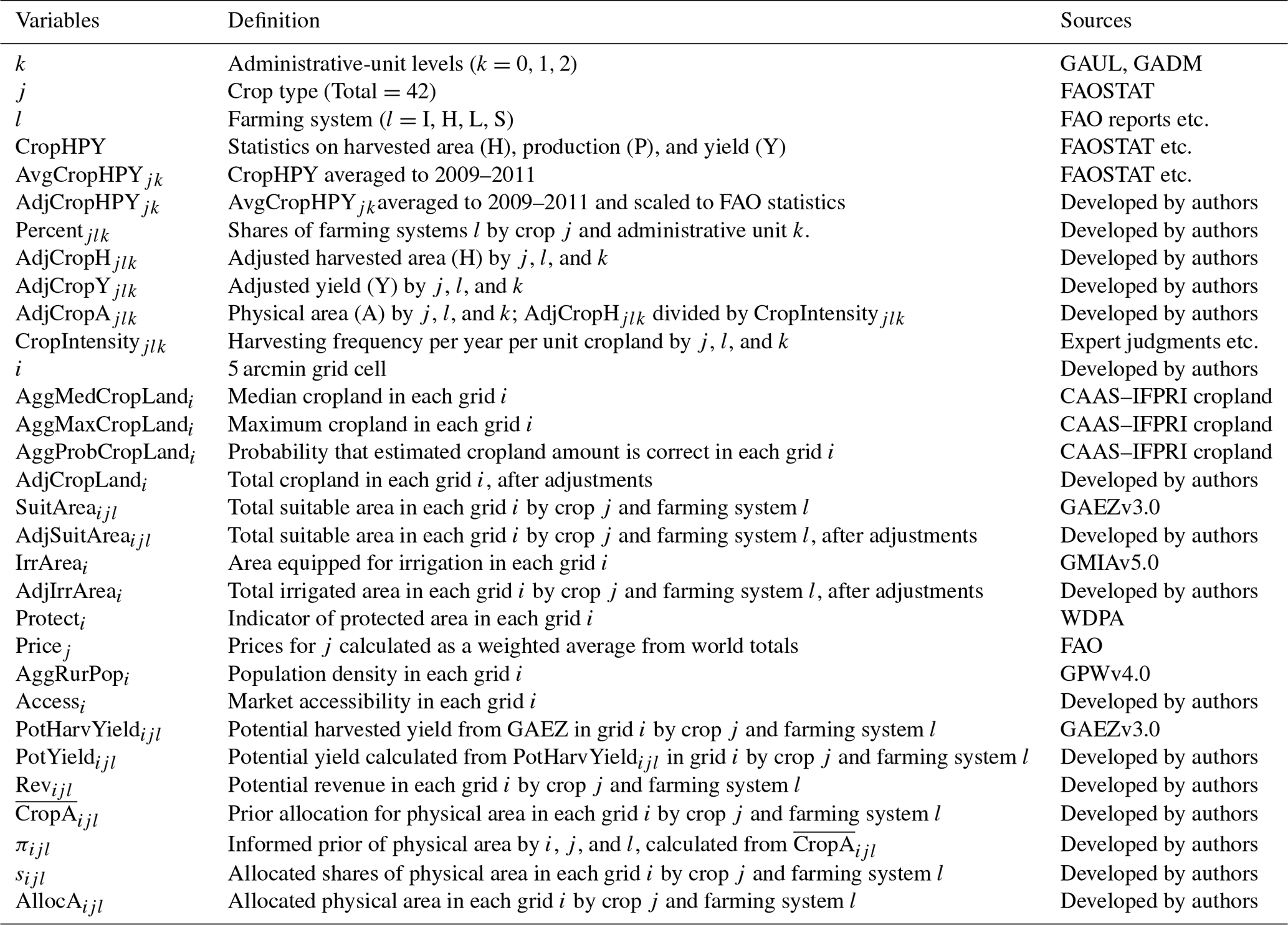
Source: developed by authors.

4.3.2 Adjusting allocation results

The model produces the allocated harvested area (AllocH_ijl), the allocated yield (AllocY_ijl), and the production quantity (AllocP_ijl) for SPAM2010. As a final step, we need to adjust the allocation results in order to keep the grid-level results consistent with the statistics. In each step of estimation, we scale the results to the national 2009–2011 FAO average (AvgCropHPY_jk0) by crop j and country k₀ to even out potential inaccuracies introduced by the allocation adjustments. This means all the allocated results in this subsection could be adjusted (if necessary) before being applied in the next phase.

We first scale the allocated harvested area (AllocH_ijl) to the national FAO average to even out potential inaccuracies introduced by the allocation adjustments:

$$\begin{array}{}\text{(19)}& \begin{array}{rl}& {\mathrm{AdjAllocH}}_{ijl}={\displaystyle \frac{{\mathrm{AllocH}}_{ijl}}{{\sum }_{i\in k_{\mathrm{0}}}{\sum }_l{\mathrm{AllocH}}_{ijl}}}\\ & \times {\mathrm{AvgFAOCropH}}_{j{k}_{\mathrm{0}}}.\end{array}\end{array}$$

Total harvested area of each crop in the grid was calculated by summing estimates across the four farming systems:

$$\begin{array}{}\text{(20)}& {\mathrm{djAllocH}}_{ij}={\sum }_l{\mathrm{AdjAllocH}}_{ijl}\forall l.\end{array}$$

For yield, we begin with the potential harvested yields (PotHarvYield_ijl) developed earlier (see Sect. S12 in the Supplement). Missing values were filled in sequentially using the following values in order of availability.

• i.

  Potential yield from potential-suitability surfaces:

  $$\begin{array}{}\text{(21)}& {\mathrm{AdjPotYield}}_{ijl}={\mathrm{PotHarvYield}}_{ijl};\end{array}$$
• ii.

  Average potential yield in SRU:

  $$\begin{array}{}\text{(22)}& \begin{array}{rl}& {\mathrm{AdjPotYield}}_{ijl}=\\ & {\displaystyle \frac{{\sum }_{i\in k_{\mathrm{SRU}}}\left({\mathrm{PotHarvYield}}_{ijl}\times {\mathrm{AdjSuitArea}}_{ijl}\right)}{{\sum }_{i\in k_{\mathrm{SRU}}}{\mathrm{AdjSuitArea}}_{ijl}}};\end{array}\end{array}$$
• iii.

  Subnational yield by crop j, input l, and ADM2 unit k₂:

  $$\begin{array}{}\text{(23)}& {\mathrm{AdjPotYield}}_{ijl}={\mathrm{AdjCropY}}_{jl{k}_{\mathrm{2}}};\end{array}$$
• iv.

  Subnational yield by crop j, input l, and ADM1 unit k₁:

  $$\begin{array}{}\text{(24)}& {\mathrm{AdjPotYield}}_{ijl}={\mathrm{AdjCropY}}_{jl{k}_{\mathrm{1}}};\end{array}$$
• v.

  National yield by crop j, input l, and ADM0 unit k₀:

  $$\begin{array}{}\text{(25)}& {\mathrm{AdjPotYield}}_{ijl}={\mathrm{AdjCropY}}_{jl{k}_{\mathrm{0}}}.\end{array}$$

Then we modify the allocated yield (AllocY_ijl) according to the minimum and maximum yields in the administrative unit:

$$\begin{array}{}\text{(26)}& \begin{array}{ll}{\mathrm{ModAllocY}}_{ijl}={\mathrm{MinYield}}_{jl{k}_{\mathrm{SRU}}}& \text{if}{\mathrm{AllocY}}_{ijl}<{\mathrm{MinYield}}_{jl{k}_{\mathrm{SRU}}}\\ {\mathrm{ModAllocY}}_{ijl}={\mathrm{MaxYield}}_{jl{k}_{\mathrm{SRU}}}& \text{if}{\mathrm{AllocY}}_{ijl}>{\mathrm{MaxYield}}_{jl{k}_{\mathrm{SRU}}}\\ {\mathrm{ModAllocY}}_{ijl}={\mathrm{AllocY}}_{ijl}& \text{if}{\mathrm{MinYield}}_{jl{k}_{\mathrm{SRU}}}\le {\mathrm{AllocY}}_{ijl}\\ & \le {\mathrm{MaxYield}}_{jl{k}_{\mathrm{SRU}}}.\end{array}\end{array}$$

For production quantity, we scale the AllocP_ijl to the national FAO average:

$$\begin{array}{}\text{(27)}& {\mathrm{AdjAllocP}}_{ijl}={\displaystyle \frac{{\mathrm{AllocP}}_{ijl}}{{\sum }_{i\in k_{\mathrm{0}}}\sum _l{\mathrm{AllocP}}_{ijl}}}\times {\mathrm{AvgCropP}}_{j{k}_{\mathrm{0}}}.\end{array}$$

Then we calculate the total production in the grid by summing overall production levels:

$$\begin{array}{}\text{(28)}& {\mathrm{AdjAllocP}}_{ij}={\sum }_l{\mathrm{AdjAllocP}}_{ijl},\forall l.\end{array}$$

Finally, we recalculate the allocated yield from the allocated harvested area and allocated production to effectively scale yields to the national FAO average:

$$\begin{array}{}\text{(29)}& {\mathrm{AdjAllocY}}_{ijl}={\displaystyle \frac{{\mathrm{AdjAllocP}}_{ijl}}{{\mathrm{AdjAllocH}}_{ijl}}}.\end{array}$$

To simplify, the grid-cell yield is calculated from the reported yield at the statistical reporting unit, the allocated area from model results, and the potential yield (at grid-cell level) from GAEZ (Global Agroecological Zone). These are illustrated in Eqs. (15) and (16): the spatial variation in yield within a statistical reporting unit follows the same spatial variation in the potential yield of that crop. In other words, the more suitable (higher potential yield) cells would have a relatively higher yield while the average yield of all the grid cells would be equal to the statistically reported yield of the administrative unit.

5 Results

In this section, we briefly showcase some of the main SPAM2010 results, which mainly focus on the staple crops, to illustrate how SPAM2010 has been produced.

5.1 Disaggregated crop statistics

Disaggregation of crop statistics is the first step for running the SPAM model. Table 3 summarizes the disaggregated rice harvested area and yield (area-weighted) for global rice production by four farming systems in SPAM2010. At the global level, the world has harvested about 160×10⁶ ha of rice around 2010. The majority of rice production area is irrigated, i.e., about 98×10⁶ha, which accounts for 61.2 % of the total rice harvested area. This share is followed by the high-input rainfed farming system (17.3 %, approximately 27 million ha), subsistence farming system (16.0 %, approximately 26 million ha), and low-input rainfed farming system (5.5 %, approximately 9 million ha). The global-average rice yield is 4374 kg∕ha, which stands at the average yield between the irrigated farming system (5528 kg∕ha) and high-input rainfed farming system (3663 kg∕ha) and is much higher than the average yield of low-input rainfed farming system (1810 kg∕ha) and the average yield of subsistence farming system (1604 kg∕ha). At the regional level, Asia (South Asia, South East Asia, East Asia together) is the largest rice-producing region, which has harvested approximately 142 million ha of rice around 2010. The majority of Asian rice production area is also irrigated, and the share, i.e., 63.7 %, is close to the global share of irrigated rice farming system. South Asia has more rice area harvested (approximately 60 million ha) than South East Asia (approximately 49 million ha) and East Asia (approximately 33 million ha). However, the average rice yield in South Asia (3553 kg∕ha) is lower than South East Asia (4125 kg∕ha) and East Asia (6566 kg∕ha). Consequently, the total rice production in these regions is very close to each other. Rice production in North America is completely irrigated, and the average yield is relatively high in this region. Subsistence rice production is mainly in sub-Saharan Africa (SSA) and South Asia, and the rice yield under subsistence conditions is also the lowest among the four farming systems.

Table 3 Regional values for area and yield of rice from SPAM2010. Unit: area (1000 ha); yield (kg∕ha).

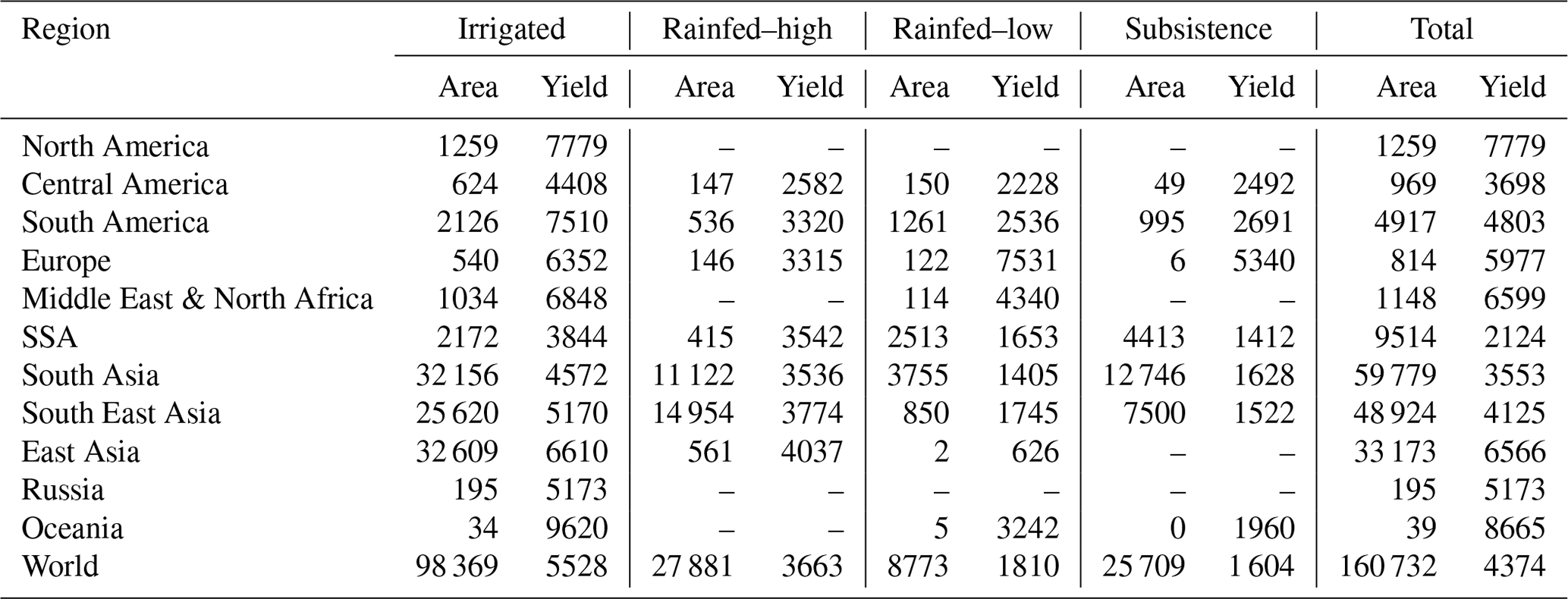
Source: developed from our own calculations.

5.2 Allocated harvested area and yield

After applying the optimization model in GAMS, the disaggregated crop statistics are spatially allocated to produce the SPAM maps. Figures 3 and 4 present the maps of harvested area and yield (after adjustment) for maize, respectively. For all farming systems, as shown in Fig. 3e, maize area is highly concentrated in northern China and North America. However, maize production in North America is mainly rainfed with high input, while in China, the rainfed farming system is mainly located in the northeastern part (Fig. 3e), and the irrigated farming system is mainly found in the north-central part (Fig. 3a). The rainfed low-input farming system (Fig. 3c) and subsistence farming system (Fig. 3d) for maize production are mainly located in South America and SSA, while the rainfed high-input maize farming system is also widely distributed outside China and northern America, including Central America, Europe, and other regions (Fig. 3b). As shown in Fig. 4e, the average maize yield is very high in North America and Europe and is relatively high in South America and Asia.

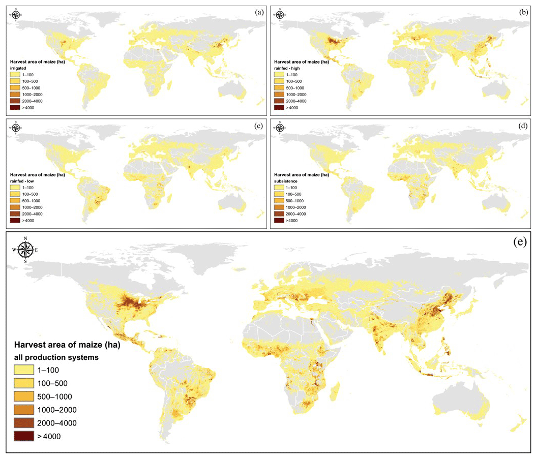
Figure 3 Harvested-area maps for maize in irrigated (a), rainfed–high (b), rainfed–low (c), subsistence (d), and all (e) farming systems.

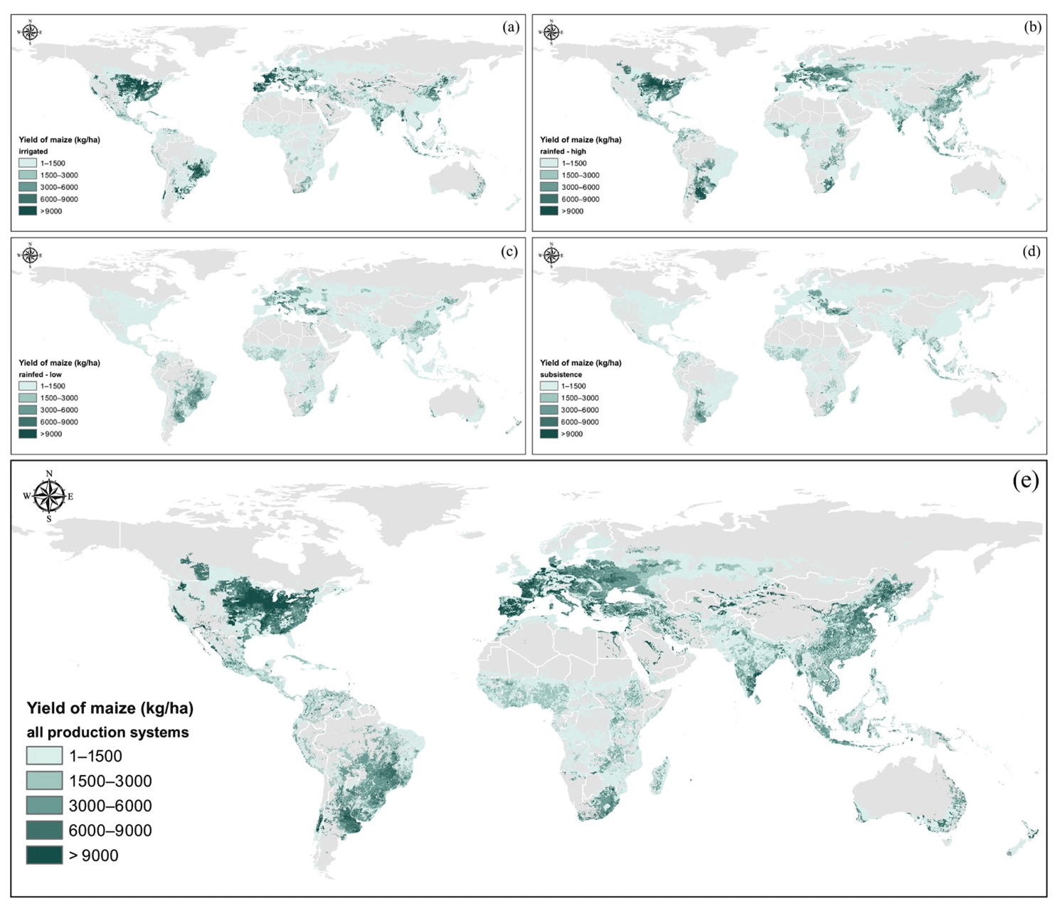
Figure 4 Yield maps for maize in irrigated (a), rainfed–high (b), rainfed–low (c), subsistence (d), and all (e) farming systems.

6 Value of production

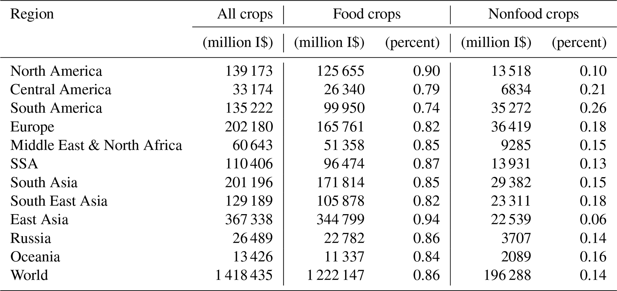
Finally, we use the average 2009–2010 base year price (international dollar, I$) to compute value of production in each grid and for each crop and farming system. Table 4 shows value of production for all crops, food and nonfood crops in all regions, and the percentage of each category value in relation to the total value. Asia (South Asia, South East Asia, East Asia together) accounts for nearly half (49.2 %) of the total value of crop production in 2010, while the Middle East and North Africa, Central America, Russia, and Oceania account for less than 5 % each. Globally, food crops account for 86.2 % of the total crop production value, with minor regional differences (the classification of crops into food and nonfood is detailed in Table S3).

Table 4 Value of production for all crops as well as food and nonfood crops in various regions.

Source: developed from our own calculations.

7 Data availability

The SPAM2010 provides four essential output indicators, including the following.

• a.

  PHYSICAL AREA: it is measured in hectares and represents the actual area where a crop is grown, not counting how often production was harvested from it. Physical area is calculated for each production system and crop, and the sum of all physical areas of the four production systems constitutes the total physical area for that crop. The sum of the physical areas of all crops in a pixel may not be larger than the pixel size.

• b.

  HARVESTED AREA: also measured in hectares, harvested area is at least as large as physical area but sometimes more since it also accounts for multiple harvests of a crop on the same plot. Like for physical area, the harvested area is calculated for each production system, and the sum of all harvested areas of all production systems in a pixel amounts to the total harvested area of the pixel. The sum of all the harvested areas of the crops in a pixel can be larger than the pixel size.

• c.

  PRODUCTION: for each production system and crop, production is calculated by multiplying area harvested by its corresponding yield. It is measured in metric tons. The total production of a crop includes the production of all production systems of that crop.

• d.

  YIELD: it is a measure of productivity, the amount of production per harvested area, and is measured in kilograms per hectare. The total yield of a crop, when considering all production systems, is not the sum of the individual yields but the weighted average of the four yields.

The SPAM2010 can be downloaded from the Harvard Dataverse (https://doi.org/10.7910/DVN/PRFF8V; IFPRI, 2019), which includes all results of maps, tables, and figures. Registered users can find more information for the SPAM model and the previous versions of SPAM datasets via the dedicated MapSPAM website (http://mapspam.info/, last access: 11 December 2020). The formal SPAM products in 2000 and 2005 are also available on the MapSPAM website. Their Dataverse addresses are https://doi.org/10.7910/DVN/A50I2T (SPAM, 2000) and https://doi.org/10.7910/DVN/DHXBJX (SPAM, 2005). All these three datasets are in the same place grouped under IFPRI Harvest Choice Dataverse (https://dataverse.harvard.edu/dataverse/harvestchoice, last access: 11 December 2020).

8 Discussion

8.1 Model uncertainty and validation

The first SPAM product was the regional-level agricultural-production maps produced for Brazil circa 1994 (You et al., 2006). Since then the model and products of SPAM have been continuously improved and updated. Besides the evolution of the method (see Sect. 3), the evaluation of SPAM model performance is also improving. In one of our early works, the uncertainty in the model, i.e., the variance explained by the cross-entropy approach, is evaluated by comparing it with the performance of simplified proportional approaches, which have been used by Monfreda et al. (2008) for producing the M3 dataset. It was proven that the cross-entropy approach was more successful in estimating crop areas than the proportional approaches, no matter the proportion to the total land area, to the cropland area, or to the amount of (biophysically) suitable land for the production of each crop (You et al., 2006). Moreover, many researchers believed that the inclusion of economic factors, i.e., market, would increase the performance of the crop disaggregation model (see the discussion in You et al., 2014), though it does not automatically guarantee that model's outputs. This partly explained the considerable discrepancies between SPAM2000 and M3 (Anderson et al., 2015) and partly confirmed that using more sophisticated approaches for production allocation would reduce uncertainty (Donaldson and Storeygard, 2016). In one of our recent works, the sensitivity of the variant of the standard SPAM model output to a few methodological-data choices had been evaluated. These include the spatial allocation method, the crop coverage, the treatment of a “rest-of-crops” aggregate, the incorporation of a “crop potential suitability” data layer, the inclusion of rudimentary economic elements, and the administrative-unit details of the primary source statistics. It showed that the standard SPAM estimates are unsensitive to the inclusion of crude economic elements, moderately sensitive to the set of crops or crop aggregates being modeled, and mostly dependent on the degree of disaggregation of the underlying national and subnational production statistics (Joglekar et al., 2019). This implies that the improvements to the methodological aspect of SPAM have limited effect on reducing uncertainty. By contrast, the quality and accuracy of the underlying statistics used to prime the model are particularly pertinent (Joglekar et al., 2019).

SPAM products are estimates with various uncertainty. Inaccuracy surely exists and varies from region to region and even from crop to crop. Although there were efforts paid to the evaluation of model conceptualization and performance, those previous validations should not be taken for granted for the latest updates. Therefore, we carried out extensive validation work to assess the accuracy of the output maps of SPAM2010. Firstly, we relied on a system through which we are able to send the crop maps to collaborators and users alike for comments or assessment. For example, the CGIAR is a global partnership which unites 15 centers engaged in agricultural research. Each center has its own mandate crops, e.g., IRRI (International Rice Research Institute) for rice and CIMMYT (International Maize and Wheat Improvement Center) for maize and wheat. We took advantage of their vast network of field offices and local expertise to help us to validate the SPAM results. Many researchers from these institutes have been involved in the production of SPAM2010, which increases the reliability of the results. The Chinese Academy of Agricultural Sciences (CAAS) undertook the regional-level validation for SPAM2010 following the approaches they have applied for the evaluations of previous SPAM products (Liu et al., 2013; Li et al., 2016; Chen et al., 2016). Moreover, field-level validating information has either been collected by crowdsourcing tools such as Geo-Wiki (Fritz et al., 2012) and eFarm (Yu et al., 2017a) or through field trips and workshops on-site or online, where local experts were asked to confirm or validate the crop production maps by providing handwritten comments or posting comments online at the our MapSPAM website. Most of these reports were collected crop by crop and country by country. An example of the detailed validation process is provided in the Supplement (see Sect. S16). The complete validation process could take a great deal of effort and time, but these users' feedback is quite important and valuable. We took this feedback and rerun SPAM model and further released the updated versions of SPAM. The previous SPAM products have been updated substantially with the help of those comments. For example, SPAM2000 and SPAM2005 are at version 3.07 and version 3.20, respectively. The current product, i.e., SPAM2010v1.10, was already released after extensive validations; it is still open and ready to receive more comments. Such an iterative process would enable a continued update to improve the product quality.

Secondly, we qualitatively evaluated the uncertainty in the input data. Like any models, the results depend on the input data and the modeling process. For SPAM, the most important input data are the subnational crop data, which have a large impact on the final product accuracy as mentioned before. We built our SPAM uncertainty rating mainly on the availability and confidence of our subnational data. In addition, we added the parameters and constraints we have to adjust to solve the SPAM model. For example, we sometimes have to abandon some crop-potential-suitability constraints in order to solve a country. For some countries, we may have to allow cropland per pixel to increase by 5 % or even 10 % of the original input to make the model run. In addition, we collected feedback and comments from users, local experts, and collaborators as discussed above. They are sporadic but very useful. We combine all the information together to give a subjective rating on how confidence we, the SPAM team, think of our final crop maps (both area and yield) based on the judgment of the reliability of input data. Figure 5 shows the country-level uncertainty rating with 5 categories (1 represents the lowest uncertainty, 5 the highest). The complete rating list is presented in Sect. S17 in the Supplement. Not surprisingly, the uncertainty in Africa and South East Asia is higher than that in countries in Europe and America. Although such a validation process is not vigorous, the result is convincing, and such a rating is highly demanded and explicitly requested by users.

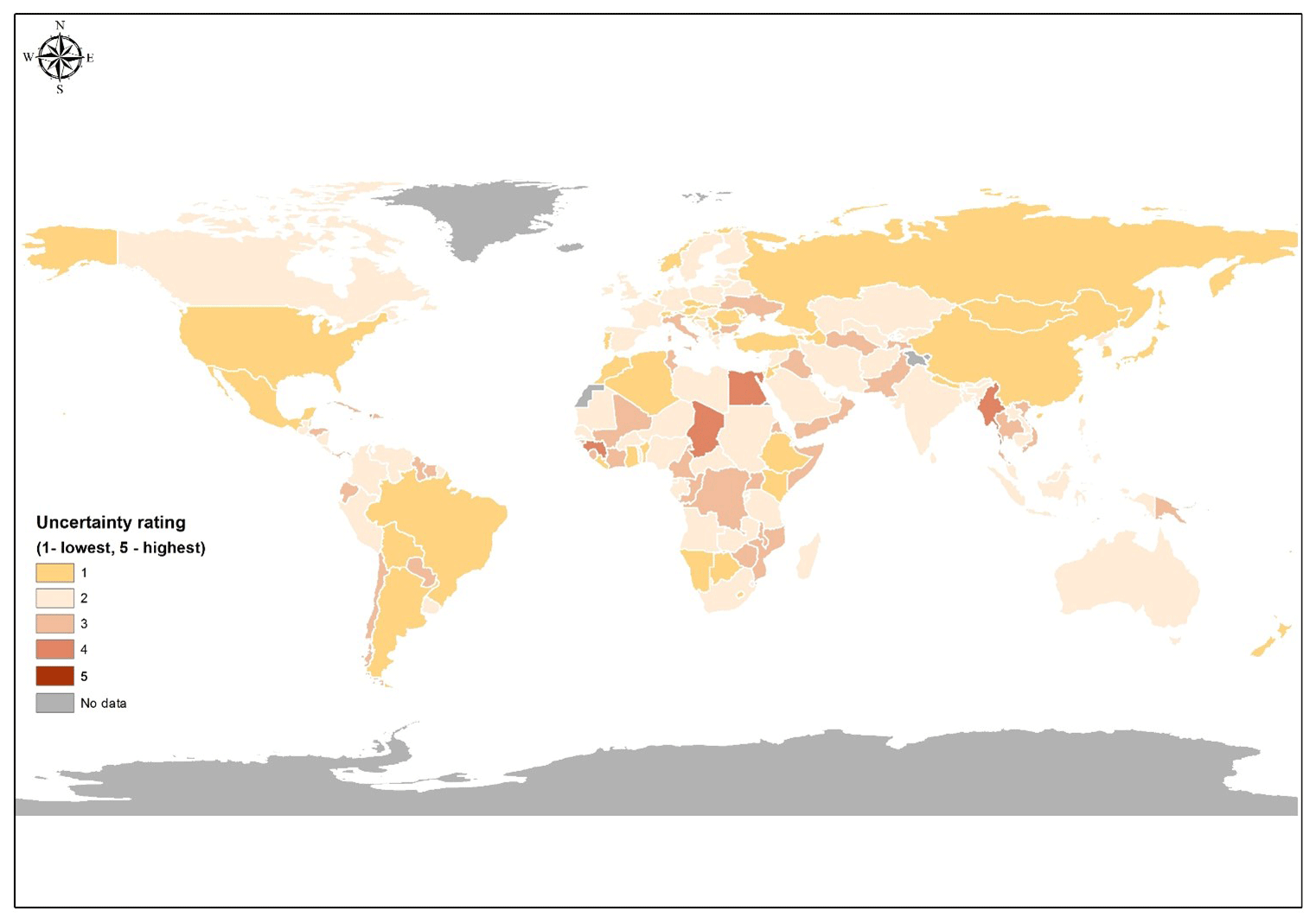
Figure 5 Subjective uncertainty rating for SPAM2010 input data by individual countries.

Thirdly, we quantitatively evaluated the results by cross-comparing the results with statistics at another administrative level that has not been used in running the model. We ran SPAM with complete statistics (ADM0, ADM1, and ADM2) and then ran them with only ADM0 and ADM1 statistics to see how the aggregated results to ADM2 compare to the original statistics at ADM2, or at least to the aggregated original results at ADM2. The runs were all done at ADM1 and then combined to give results for the whole country. We then calculated the coefficient of determination (R²) between the values allocated from model and obtained from statistics to assess the model performance. In general, a higher R² indicates a better performance. This approach has already been used for evaluating the performance of SPAM2000 (You et al., 2014). The upper part of Fig. 6 shows the results of such an approach applied to Brazil in SPAM2000 for its main food crops, while the bottom part of Fig. 6 shows the results of the same approach applied to the same country for the same crops in SPAM2010. The figure clearly indicates that the model performed better in allocating rice than other crops. Moreover, the performance improved greatly from SPAM2000 to SPAM2010, especially for soybean and potato. We further selected a few smaller countries in Asia and Africa to undertake the same assessment, which are believed to have a relatively higher uncertainty in terms of input data (Fig. 5). Bangladesh, Benin, Senegal, and Tanzania were selected as they have good statistical data coverage in SPAM2010. Figure 7 shows that the R² for selected crops (i.e., maize, rice, and cotton) ranged between 0.66 and 0.94, suggesting that the overall performance of SPAM2010 is good in these selected countries for those selected crops.

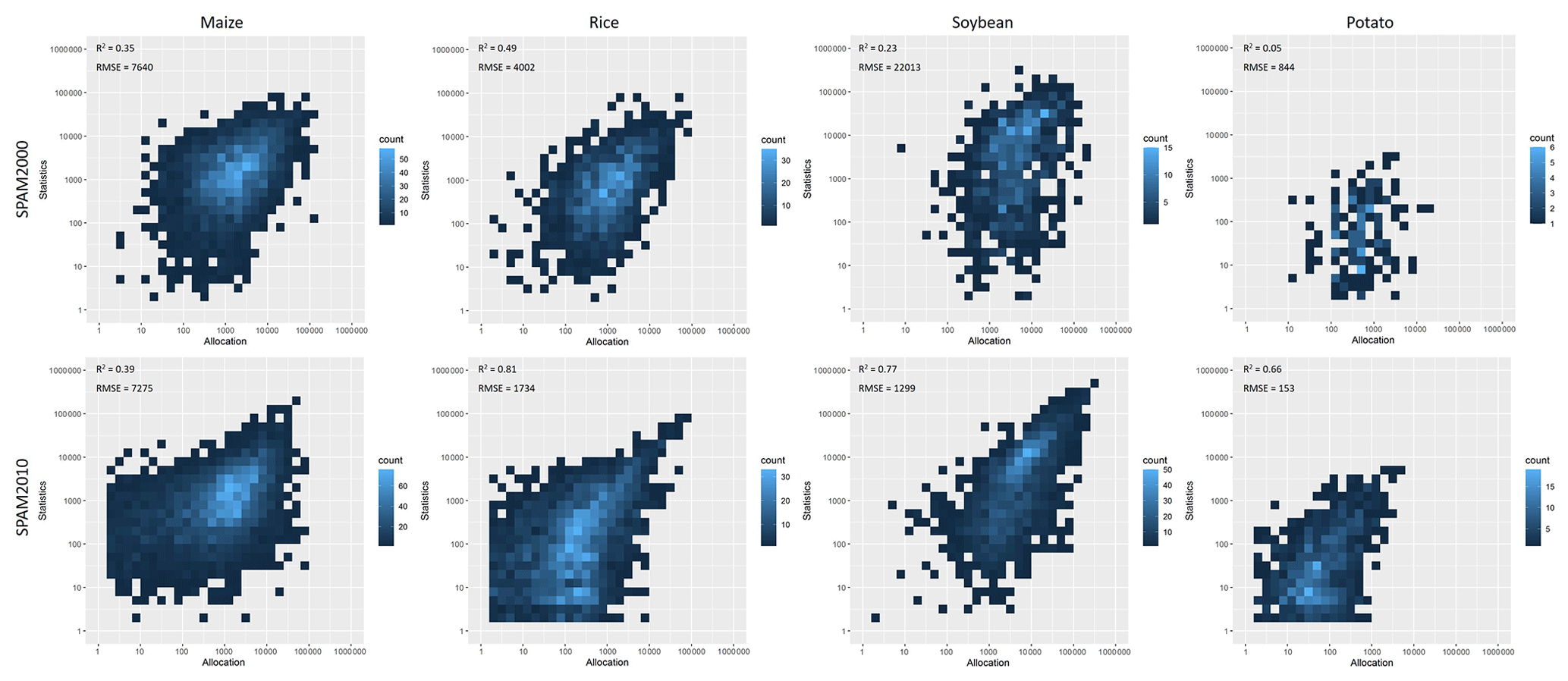
Figure 6 Comparison between the allocated crop area and statistics crop area at the ADM2 level in Brazil (log–log scale plot; unit: ha). The upper part is for SPAM2000 and the bottom part is for SPAM2010.

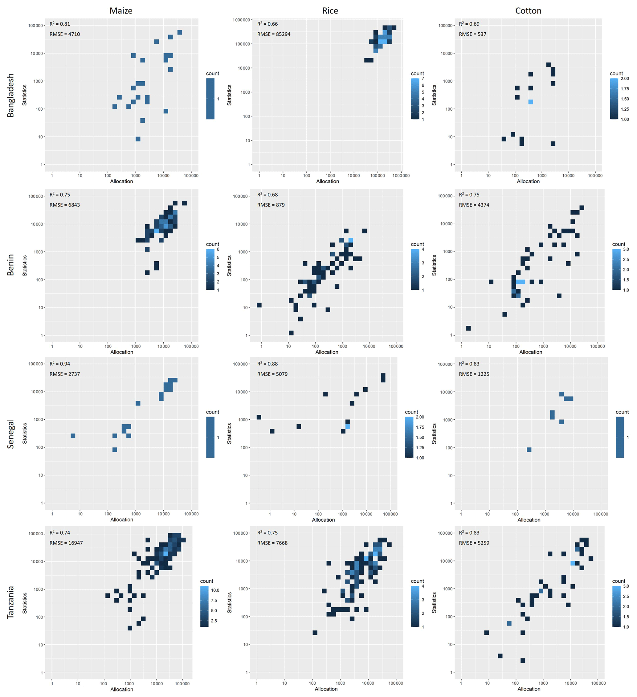
Figure 7 Comparison between the allocated crop area and statistics crop area at the ADM2 level in Bangladesh, Benin, Senegal, and Tanzania for maize, rice, and cotton (log–log scale plot; unit: ha).

Finally we did regional-level quantitative validations when third-party independent crop maps were available, given that it is impossible for us to collect the true spatial distribution of crops (both area and yield) for the time of 2010 on a global scale. Among the limited third-party independent spatial crop distribution data, the Cropland Data Layer (CDL; https://nassgeodata.gmu.edu/CropScape/, last access: 11 December 2020) is a crop-specific land cover dataset created for the continental United States using moderate-resolution satellite imagery and extensive agricultural ground truth, which has been applied to validate our SPAM2010 product at the regional scale by correlating the grid-level crop area. We focus on the three most popular staple crops in the United States, i.e., maize, wheat, and soybean, and obtain the crop area maps of 2009, 2000, and 2011 from CDL. We calculate the 2009–2011 average crop areas at a 5 arcmin resolution for CDL according to the scheme of SPAM2010 and further calculate the coefficient of determination (R²) and the root mean square error (RMSE) between the grid-level values derived from the two datasets (Fig. 8). The values of R² are between 0.71 and 0.91, and the values of RMSE are between 231 and 307 ha, indicating a relatively high reliability. In particular, the higher R² and lower RMSE suggest our maize and soybean maps are more reliable than the wheat map. There are potentially many factors affecting the different results if we treat CDL as the truth, for example, the different accuracy or availability of input data, suitability layers, and parameters for the area shares and yield ratios. Another possible reason is that we did not distinguish spring wheat and winter wheat in SPAM, which partly explains why the agreement for wheat is lower than that for maize and soybean. Moreover, the National Land Cover Dataset (NLCD) of China mapped paddy field distribution as a special cropland cover at a 1 × 1 km grid level (http://www.resdc.cn/data.aspx?DATAID=99, last access: 11 December 2020). By assuming paddy fields will be mostly used for growing rice, we evaluate the rice area map in China by correlating SPAM2010_rice and NLCD2010_paddy according to the same scheme described above. The value of R² is 0.49, and the value of RMSE is 1024 ha (Fig. 9). Although this result does not seem as good as the results from the United States by using CDL, it is fairly acceptable because NLCD measures land cover rather than land use and is in a relatively coarse spatial resolution. Moreover, the R² is substantially increased comparing to its predecessors. For example, the R² is assessed as 0.42 for SPAM2005 by using the same approach according to Liu et al. (2013). In addition, there are regional-level crop distribution maps produced by independent efforts on interpreting remotely sensed images. For example, Zhang et al. (2017) provided annual paddy area time series from 2000 to 2010 based on satellite remote sensing for China and India. We compared these remote-sensing-derived paddy maps with the rice area estimated by SPAM for the year 2010. The R² values are 0.36 and 0.34 for China and India, respectively (Fig. 10). We could expand this quantitative evaluation when more third-party independent crop maps are available. However, it should be noted that errors might exist in the third-party independent crop maps as well; hence this quantitative evaluation approach also might result in uncertainty. Our results show that the uncertainty gradually increases when applying CDL, NLCD, and Zhang et al. (2017).

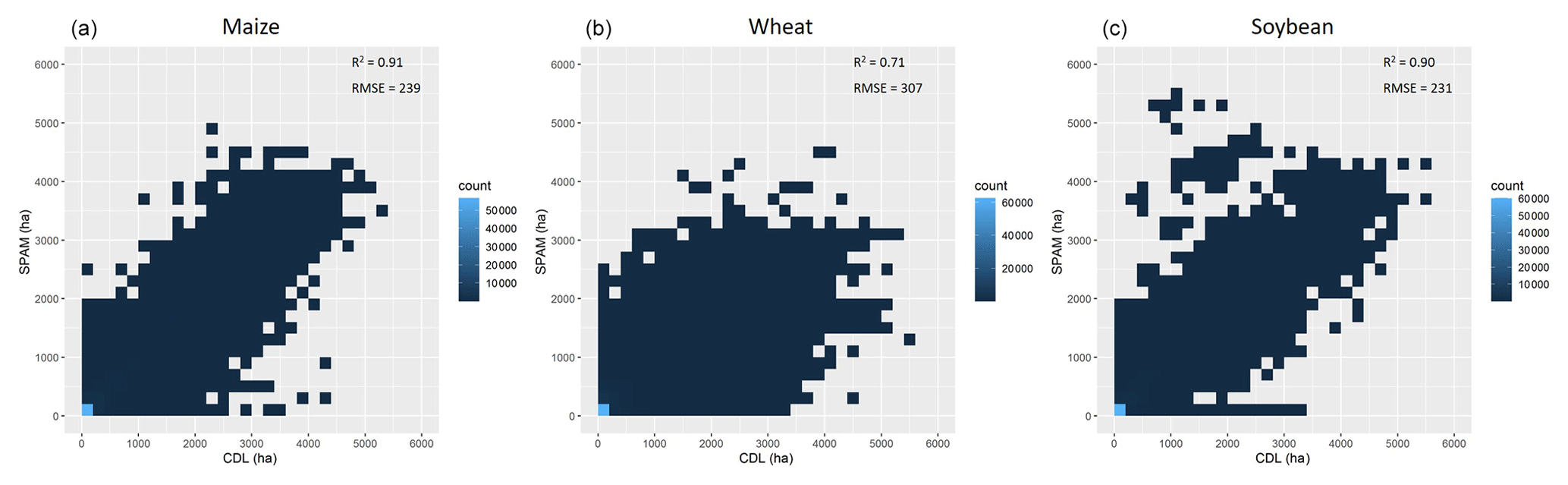
Figure 8 Grid-by-grid comparison of crop area for maize (a), wheat (b), and soybean (c) between SPAM2010 and CDL2010 in the continental US.

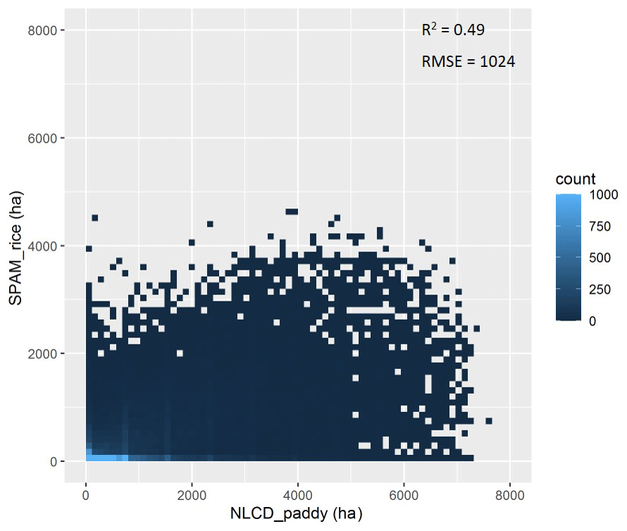
Figure 9 Grid-by-grid comparison between SPAM2010 rice area and NLCD2010 paddy field area in China.

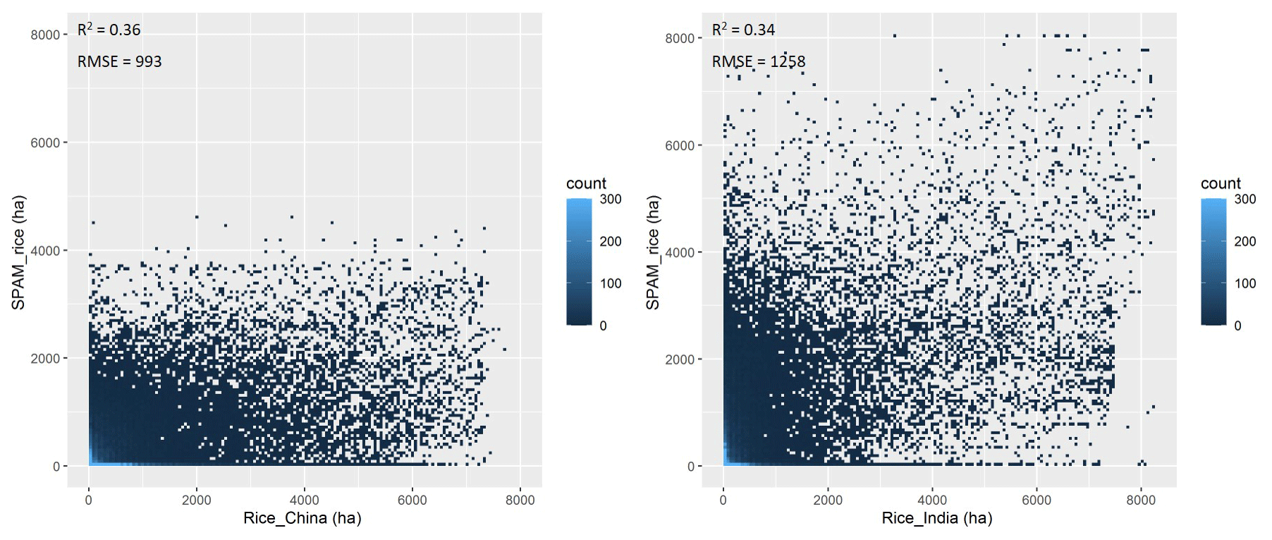
Figure 10 Grid-by-grid comparison between SPAM2010 and Zhang et al. (2017) rice area in China and India.

8.2 Data comparison

There are a few reports which compare SPAM with M3, MIRCA, and GAEZ, especially their output maps circa 2000 (Anderson et al., 2015; Donaldson and Storeygard, 2016). Although it is difficult to make statements about which one is better, there are several features that distinguish SPAM products from the M3, MIRCA, and GAEZ data. First, the estimates from SPAM can be customized using user-provided data for one or more of the input variables and return results to the provider in a short turnaround period. Second, although SPAM runs mainly at a 5 arcmin resolution, it can be run at higher resolutions provided that at least some of the rasterized inputs also have higher-resolution data to support such an exercise. Third, considerable effort is made to compile subnational crop statistics at administrative level 2 (e.g., district or county) for all possible countries. Fourth, if there is knowledge of crop existence in any area for any crop, this can be incorporated into the model to make a more accurate crop allocation. Moreover, SPAM does not have a large coverage of crops (compared to M3) and does not include detailed biophysical parameters (compared to MIRCA and GAEZ); instead it focuses more on agricultural production by providing data on crop harvested area and yield disaggregated by farming systems. Finally, SPAM results are readily available on the internet in several formats (also tabular) for all interested users. We are currently building a SPAM model in the cloud, where we let any user supply his or her own input data and run SPAM on his or her own under the GitHub platform. This SPAM in the cloud will be published and communicated to the SPAM user community once it is ready.

Anderson et al. (2015) conclude that substantial discrepancies exist across these four global spatially explicit crop production datasets circa 2000, and the disagreement between models serves as a reminder of the ongoing challenges to the creation of spatially explicit estimates of harvested area and yield based on crop statistics. However, it is more challenging to assess the disaggregated farming system results such as irrigated rice vs. rainfed rice and subsistence maize vs. high-input rainfed rice, which have not been systematically explored in Anderson et al. (2015). We collected additional global datasets which are relevant to agricultural-production mapping, e.g., the average irrigated and rainfed yields (ca. 2000) from Siebert and Döll (2010) and the harvested area and yield for four crops (ca. 2005) from http://www.earthstat.org/ (last access: 11 December 2020). We compared these datasets with our SPAM products for the corresponding period. We found that the results are differed from crop to crop and from farming system to farming system. In general, the yield estimates on maize and wheat are better than the other crops, and the irrigated yields are better than the rainfed yields (Figs. 11 and 12).

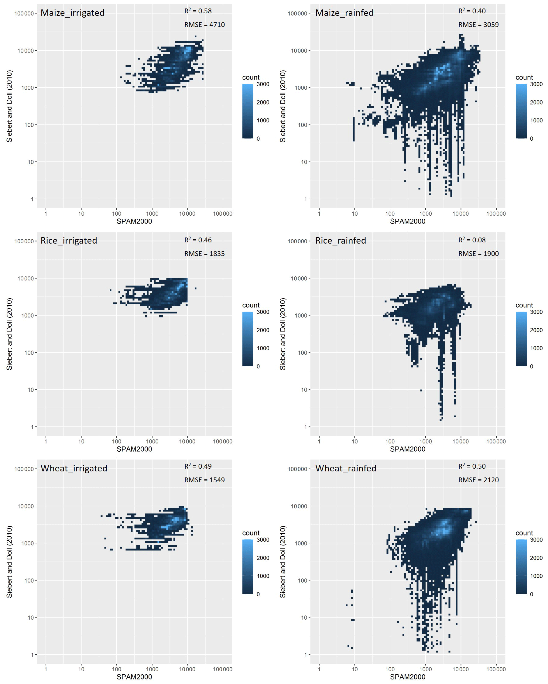
Figure 11 Grid-by-grid comparison between SPAM2000 and Siebert and Doll (2010) in average irrigated and rainfed yields (log–log scale plot; unit: kg∕ha).

Figure 12 Grid-by-grid comparison between SPAM2005 and EARTHSTAT2005 in crop yields. (log–log scale plot; unit: kg∕ha).

However, as M3, MIRCA, and GAEZ do not provide subsequent global spatially explicit crop production ca. 2000, it is impossible to compare the current SPAM2010 with other data products. In order to illustrate the continuity of SPAM products, we present a grid-by-grid comparison between SPAM2010 and SPAM2005. Figure 13 shows that rice production in 2010 increased notably in eastern Europe, Africa, northeastern China, northwestern India, southern Australia, etc., while it decreased notably in central Asia and South America. Maize production displays an overall increase across the globe between 2005 and 2010, except for some places in central Asia, which have shown a decreasing trend. It is also noticeable that maize production in the US and Europe has kept relatively stable. This result is accordant with the “maize boom” which had taken place around the globe (Herrmann, 2013), especially in the developing countries (Cairns et al., 2013; Ornetsmüller et al., 2019). It should be noted that the current type of comparison may not be a perfect comparison (because differences exist in methodologies and data input applied in SPAM2005 and SPAM2010) and that the current comparison only shows the rate of change; thus a higher value does not necessarily indicate a huge change in absolute crop production.

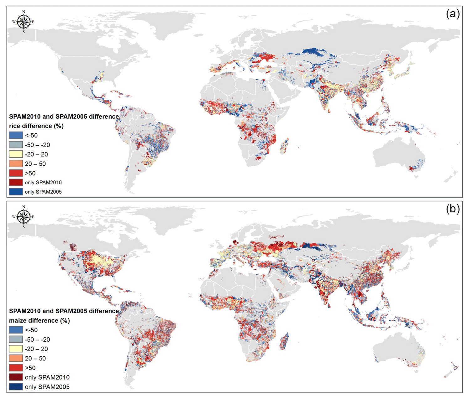
Figure 13 Comparison between SPAM2010 and SPAM2005: (a) relative difference in rice production, (b) relative difference in maize production.

In addition, we compared the changes in crop area between SPAM products and the abovementioned regional-level independent crop maps once they were available in time series. We calculated the area changes in maize, wheat, and soybean by overlaying CDL2005 and CDL2010 and undertook the same procedure for SPAM. We then plot these changes (i.e., ΔCDL and ΔSPAM) in Fig. 14. Likewise, we compared the changes in SPAM rice area and the changes in paddy rice area obtained from Zhang et al. (2017; Fig. 15). Figures 14 and 15 both show that the coefficient of determination is extremely low between changes yielded from different data products, which further reminds us that it is inappropriate to directly compare SPAM products over time, although we are confident of the spatial accuracy of SPAM products at each time stage. This is mainly because SPAM requires a large number of input data, yet the sources of these multiple data inputs cannot be guaranteed to be the same across different time stages. Therefore, such changes reflected by SPAM products over time not only mix real changes on the ground but also largely depend on the input data. For example, the cropland layers (one of the most important data inputs) are accessed from different sources to make sure the cropland data and the statistical data are adopted for the same year. We did not evaluate the continuity of these input data, which is almost impossible and is beyond the purpose of SPAM. Consequently, it is suggested to use the SPAM products with, at least, acknowledgement to the corresponding cropland layer, e.g., Lu et al. (2020) for SPAM2010. Moreover, we do not recommend users to cross-compare the SPAM products over time because the differences may have more input data errors or inaccuracies than detecting the real change on the ground.

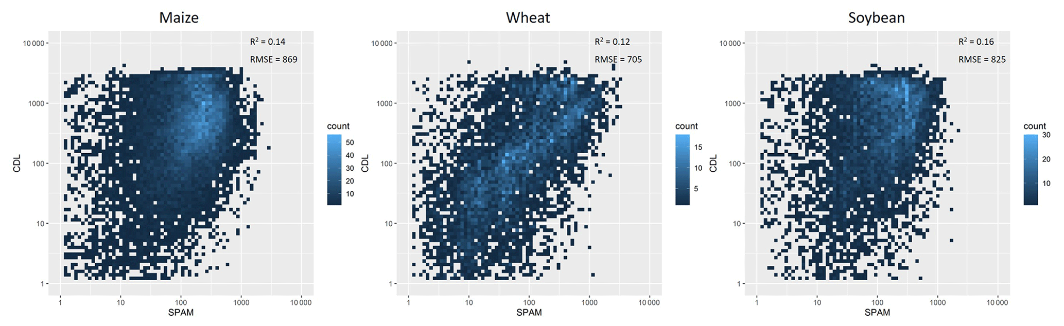
Figure 14 Comparison between SPAM crop area change and CDL crop area change (log–log scale plot; unit: ha).

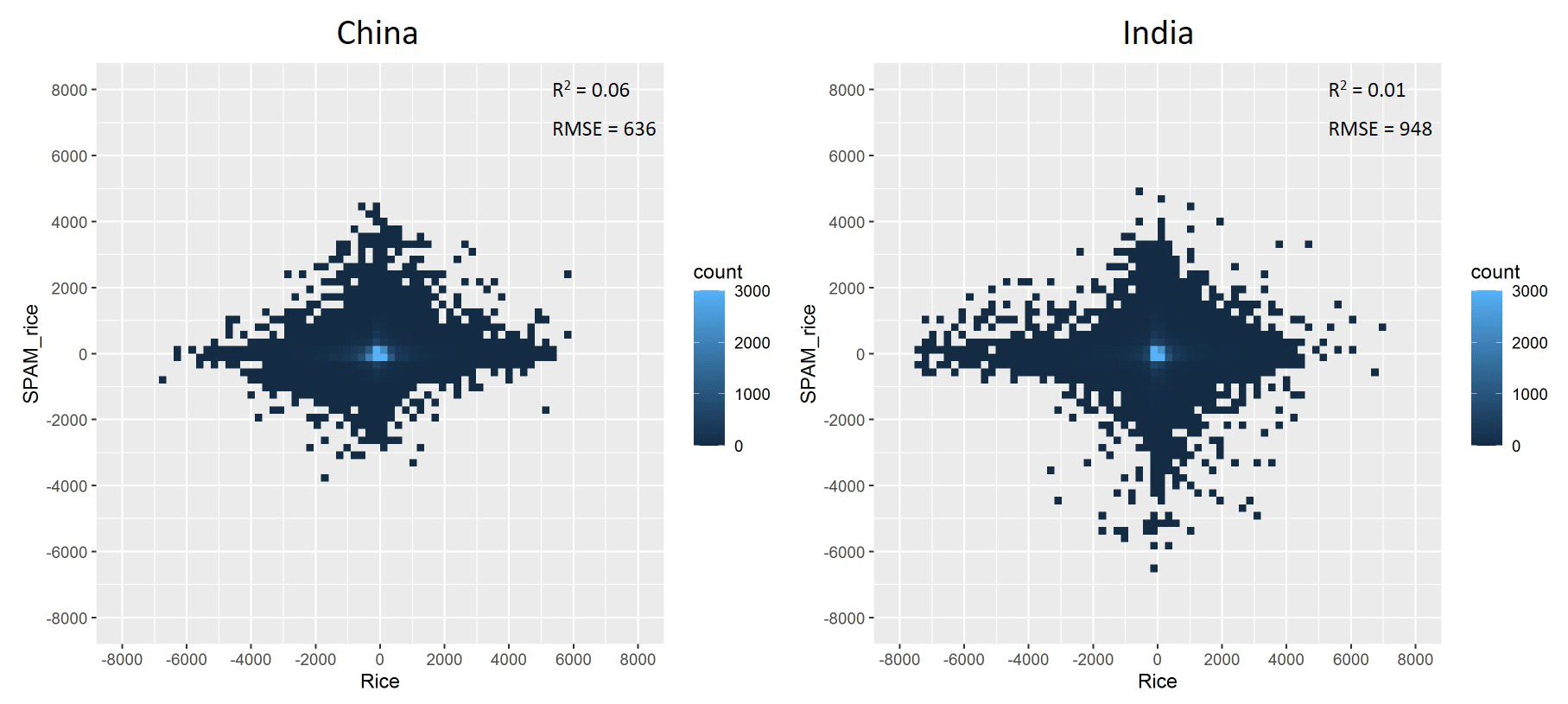
Figure 15 Comparison between SPAM rice area change and Zhang et al. (2017) paddy rice change (unit: ha).

8.3 Limitations

As stated previously, the SPAM estimates are dependent on the extent and veracity of the primary input data like most models (Joglekar et al., 2019). SPAM2010 requires data on 42 crops in over 200 countries for the production season. Ideally, these data should be collected at an ADM2 level; however this is not always possible. It is particularly difficult to a few countries such as Somali and Nigeria, where reliable data are not available, or different input data just conflict with each other. For example, only one crop area (i.e. millet) for a district is already larger than the total cropland area, yet we know there are still five more crops growing in this district. In these cases, we have to adjust the conflicting data using expert judgment to make the model solvable. Since most cropping statistics are not delineated by farming system, estimates of the shares of production under each of the four systems in question are required. To convert harvested-area statistics to the physical-area statistics used in the model, additional data on cropping intensities by crop and farming systems must be collected. We have made every effort to collect official or published data, and we reply on expert judgments as the last resort when we simply could not find other sources. For example, no country publishes official statistics on crop yield ratio (yield conversion factor) between irrigated vs. rainfed crops. We surveyed published papers, personal communication with the FAO's Agriculture to 2030 team, and gray literature to collect such data. While indeed a series of expert judgments are used, the scope (e.g., crops and regions) is quite limited in the overall input data. Once the data on disaggregate cropping practices are compiled, several variables at a gridded scale are needed to disaggregate these cropping statistics into the desired spatial units. These data include estimates of cropland, irrigated land, suitable area and yield, population density, and protected areas. The variety and sheer volume required to run the SPAM (and related) models raise questions of reliability and comprehensiveness of estimates across different cropping statistics, geographic areas, and countries.

In terms of reliability, different sources of information may lead to inconsistent and even incompatible information. For example, the data on the estimated cropland extent within a grid are compiled from several sources, which in turn deploy different methods to generate their estimates. The extent of cropland within a grid is crucial information for the allocation model, but the confidence regarding its actual location varies regionally (see Lu et al., 2020). Crop statistics on area harvested and yield may not have been consistently collected and processed across different countries, so these major data may be unreliable to begin with. Additionally, two of the major conversion factors used, farming system shares and cropping intensities, are often not available for each crop and farming system within a country. Lacking raw data on these statistics for a particular crop–country combination, these data were simply assigned from a similar crop or country or created using expert judgment. Neither data on cropping intensities nor farming system shares have been validated for reliability. In terms of comprehensiveness, notably less subnational coverage exists in developing countries, and only global-average commodity price data were used to account for the economic influences on crop production.

The wide range of data sources, coverage, and regional nuances of crop production have methodological implications. First, there are possible trade-offs between data consistency and data reliability. For example, there are requirements of the model (i.e., cropping intensities and farming system shares) that are not consistently available within a country at the administrative level needed. Often, these numbers are taken from national-level values, even though they may not reflect the reality at the administrative level. Secondly, multi- and intercropping are not handled in a sophisticated manner within SPAM. These types of cropping patterns are only accounted for using a single cropping intensity value per crop, farming system, and (possibly) subnational unit. Finally, the market is important for both subsistence farmers and commercial ones (Losch et al., 2012). In SPAM, we rely on population density for an indirect representation of market proximity. We use the rural population to calculate a prior for the subsistence portion of a crop (i.e., subsistence among the four farming systems). For subsistence farmers, by definition they mostly consume what they produce, and so we indeed assume their production is closely correlated with their rural population size. For all other farmers, we assume they produce for the market (local, regional, or even international markets). The assumption of using rural population as a proxy for market access was to break down the total cropland into individual crop areas in the prior revenue calculation. We did not, explicitly or implicitly, assume a rural population (even subsistence farmers) is entirely fed by local agriculture. Instead, we applied rural population density as a proxy for market access, which allows crop-specific tuning depending on how crops are distributed across the four farming systems. As this crop-specific revenue is divided by the total revenue within a pixel in Eqs. (9) and (10), the prior is not affected by market accessibility if it is not crop-specific. In other words, crop-specific market accessibility is preferable for the current SPAM model. Yet such accessibility data at the global scale do not exist now. We would consider including a more direct representation of market proximity by actual travel times to markets or road networks as the global roads and railways databases are becoming available (Koks et al., 2019). Several trade-offs were made to ensure that the complex allocation method was tractable, and it is important to recognize that these trade-offs likely affect the plausibility of results.

Last but not least, we admit that it is inappropriate to compare SPAM products directly across time stages (Figs. 13–15), although we have paid every effort to guarantee the spatial accuracy of SPAM products at each time stage. It is largely because the system errors exist across various data products. In a latest publication, Iizumi and Sakai (2020) released a time series product of global gridded crop yields. Although they applied a different approach (i.e., spatial adjustment) which is conceptually different from the spatial disaggregation approach applied in SPAM, it provides great implications to further integrate and standardize the SPAM and the similar gridded earth system datasets for broader applications. There is an ongoing consortium called The Land Use Change Knowledge Integration Network (LUCKiNet; http://www.luckinet.org, last access: 11 December 2020). The SPAM team is part of this consortium, which aims to integrate tools and standardize approaches across various ongoing projects that develop gridded information on land use dynamics for applications in food security, climate change, biodiversity, and other related issue areas. Not only LUCKiNet aims to create crop maps comparable over time, but we also want to have these maps consistent across land uses such as cropland, grassland, and forest. The modeling techniques would consider the spatiotemporal dynamics of different land use forms in an integrative framework.

8.4 Concluding remarks

In this paper, we present SPAM2010, the latest global gridded agricultural-production dataset in 2010. SPAM2010 uses an updated cross-entropy approach to make plausible estimates of crop distribution for 42 crops and four farming systems within disaggregated units, which shows great improvement over its predecessors: SPAM2000 and SPAM2005. For example, the expanded crop list enables the analysis for not only staple food crops but also cash crops. A recent study has analyzed the global beer supply by using SPAM2000 (Xie et al., 2018). It will be very promising to analyze the global coffee and tea supply by using the latest dataset as these crops are newly included in SPAM2010 and are in increasing demand with superior economic value but also highly sensitive to climate change (Bunn et al., 2015).

SPAM2010 substantially extends the SPAM family and fills the gap for the work of global agricultural-production mapping by successfully creating a global gridscape at the confluence between earth and farming systems. In particular, it helps to better understand land management practices characterized by concomitant data and knowledge gaps (e.g., crop selection and element of crop harvest; Erb et al., 2017). It not only allows analysts and policymakers to better target agricultural and rural development policies and investments, increasing food security and growth with minimal environmental impacts, but also enables scientists to better address the global-change challenges within the anthroposphere and beyond by providing the only possibility for updating the global agricultural and environmental assessments from 2000 (when M3, MIRCA, GAEZ, and SPAM2000 are available) to 2005 and 2010 (when SPAM2005 and SPAM2010 are available as well). All the SPAM maps and tabular data in multiple time stages are freely available on the MapSPAM website (http://mapspam.info/  last access: 11 December 2020), which also acts as a platform for validating and improving the performance of the SPAM maps by collecting feedback from users.