the Creative Commons Attribution 4.0 License.
the Creative Commons Attribution 4.0 License.
 | 18 Dec 2020
Year-round record of near-surface ozone and O3 enhancement events (OEEs) at Dome A, East Antarctica
Biao Tian
Michael C. B. Ashley
Davide Putero
Zhenxi Zhu
Lifan Wang
Shihai Yang
Chuanjin Li
Cunde Xiao
Dome A, the summit of the East Antarctic Ice Sheet, is an area challenging to access and is one of the harshest environments on Earth. Up until recently, long-term automated observations from Dome A (DA) were only possible with very low power instruments such as a basic meteorological station. To evaluate the characteristics of near-surface O3, continuous observations were carried out in 2016. Together with observations at the Amundsen–Scott Station (South Pole – SP) and Zhongshan Station (ZS, on the southeast coast of Prydz Bay), the seasonal and diurnal O3 variabilities were investigated. The results showed different patterns between coastal and inland Antarctic areas that were characterized by high concentrations in cold seasons and at night. The annual mean values at the three stations (DA, SP and ZS) were 29.2±7.5, 29.9±5.0 and 24.1±5.8 ppb, respectively. We investigated the effect of specific atmospheric processes on near-surface summer O3 variability, when O3 enhancement events (OEEs) are systematically observed at DA (average monthly frequency peaking at up to 64.5 % in December). As deduced by a statistical selection methodology, these O3 enhancement events (OEEs) are affected by significant interannual variability, both in their average O3 values and in their frequency. To explain part of this variability, we analyzed the OEEs as a function of specific atmospheric processes: (i) the role of synoptic-scale air mass transport over the Antarctic Plateau was explored using the Lagrangian back-trajectory analysis Hybrid Single-Particle Lagrangian Integrated Trajectory (HYSPLIT) method, and (ii) the occurrence of “deep” stratospheric intrusion events was investigated using the Lagrangian tool STEFLUX. The specific atmospheric processes, including synoptic-scale air mass transport, were analyzed by the HYSPLIT back-trajectory analysis and the potential source contribution function (PSCF) model. Short-range transport accounted for the O3 enhancement events (OEEs) during summer at DA, rather than efficient local production, which is consistent with previous studies of inland Antarctica. Moreover, the identification of recent (i.e., 4 d old) stratospheric-intrusion events by STEFLUX suggested that deep events only had a minor influence (up to 1.1 % of the period, in August) on deep events during the variability in near-surface summer O3 at DA. The deep events during the polar night were significantly higher than those during the polar day. This work provides unique data on ozone variation at DA and expands our knowledge of such events in Antarctica. Data are available at https://doi.org/10.5281/zenodo.3923517 (Ding and Tian, 2020).
- Article
(4137 KB) - Full-text XML
- Companion paper
-
Supplement
(170 KB) - BibTeX
- EndNote


Ozone (O3) is a natural atmospheric component that is found in both the stratosphere and the troposphere and plays a major role in the atmospheric environment through radiative and chemical processes. O3 does not have direct natural sources such as emission from the ground or vegetation but rather is produced in the atmosphere, and its concentration ranges from a few parts per billion near the Earth's surface to approximately a few parts per million in the stratosphere. Stratospheric O3, which is produced as a result of the photolysis of molecular oxygen, forms a protective layer against the UV radiation from the sun. By contrast, throughout the troposphere and at the surface, O3 is considered a secondary short-lived air pollutant (Monks et al., 2015), and O3 itself is a greenhouse gas, such that a reduction in concentration has a direct influence on radiative forcing (Mickley et al., 1999; IPCC, 2013; Stevenson et al., 1998).
O3 photochemical production in the troposphere occurs via hydroxyl radical oxidation of carbon monoxide (CO), methane (CH4) and non-methane hydrocarbons (generally referred to as NMHCs) in the presence of nitrogen oxides (NOx) (Monks et al., 2015). As these precursors are localized and their lifetimes are generally short, the distribution of near-surface O3, which is produced from anthropogenic precursors, is also localized and time-variant. In the presence of strong solar radiation with λ<424 nm, volatile organic compounds (VOCs) and NOx (NO+NO2), O3 is photochemically produced and can accumulate to reach a hazardous level during favorable meteorological conditions (Davidson, 1993; Wakamatsu et al., 1996). In the case of NOx-rich air, NO2 is produced and accumulates via the reaction between NO and HO2 or RO2 (peroxy radicals), which is followed by the accumulation of O3. However, in the case of NOx-poor air, these proxy radicals react with O3 and lead to O3 loss (Lin et al., 1988). Experiments conducted in Michigan (Honrath et al., 2000a) and Antarctica (Jones et al., 2000) found that NOx can be produced in surface snow. This production appears to be directly driven by incident radiation and photolysis of nitrate deposited in the snow (Honrath et al., 2000a, b).
Previous studies have shown that the near-surface O3 of Antarctica may be influenced by a number of climate-related variables (Berman et al., 1999), such as the variation in UV flux caused by the variation in O3 column concentration over Antarctica (Jones and Wolff, 2003; Frey et al., 2015); the accumulation and transport of long-distance, high-concentration air masses (e.g., Legrand et al., 2016); and the depth of continental mixing layers. Many studies have observed summer episodes of “O3 enhancement events” (OEEs) in the Antarctic interior (e.g., Crawford et al., 2001; Legrand et al., 2009; Cristofanelli et al., 2018), and they have attributed this phenomenon to the NOx emissions from the snowpack and subsequent photochemical O3 production (for example, Jones et al., 2000). Moreover, this may provide an input source for the entire Antarctic region (for example, Legrand et al., 2016; Bauguitte et al., 2011). As the solar irradiance and the nitrate aerosol concentration increase, the emission of NOx will increase through the photodenitrification process of the summer snowpack (e.g., ; ; Honrath et al., 2000a; Warneck and Wurzinger, 1989). Helmig et al. (2008a, b) provided further insight into the vigorous photochemistry and O3 production that result from the highly elevated levels of NOx in the Antarctic surface layer. During stable atmospheric conditions, which are typically observed during low-wind and fair-sky conditions, O3 accumulated in the surface layer can reach up to twice its background concentration. Neff et al. (2008a) showed that shallow mixing layers associated with light winds and strong surface stability can be among the dominant factors leading to high NO levels. As shown by Cristofanelli et al. (2008) and Legrand et al. (2016), the photochemically produced O3 in the planetary boundary layer (PBL) over the Antarctic Plateau can affect the O3 variability thousands of kilometers away from the emission area, due to air mass transport.
The near-surface O3 concentrations at high-elevation sites can also be increased by the downward transport of O3-rich air from the stratosphere during deep convection and stratosphere-to-troposphere transport (STT) events. Moreover, the stratospheric O3 in the polar regions can be transferred to the troposphere not only during intrusion events but also as a result of slow but prolonged subsidence (e.g., Gruzdev et al., 1993; Roscoe, 2004; Greenslade et al., 2017). The earliest studies, carried out with the aircraft flight NSFC-130 over the Ellsworth Mountains of Antarctica in 1978, found that mountainous terrain may induce atmospheric waves that propagate through the tropopause. The tropospheric and stratospheric air may be mixed, leading to an increase in the tropospheric O3 concentration (e.g., Robinson et al., 1983). Radio soundings at the Resolute and Amundsen–Scott stations also showed the existence of transport from the stratosphere to the troposphere, and the flux could reach up to 5×10¹⁰ (e.g., Gruzdev et al., 1993). Recently, Traversi et al. (2014, 2017) suggested that the variability in air mass transport from the stratosphere to the Antarctic Plateau could affect the nitrate content in the lower troposphere and the snowpack.
Currently, the climatology of tropospheric O3 over Antarctica is relatively understudied because observations of year-round near-surface O3 have been tied to manned research stations. These stations are generally located in coastal Antarctica, except for the South Pole (SP) and Dome C continental stations on the East Antarctic Plateau. Thus, the only information currently available for the vast region between the coast and plateau are spot measurements of boundary layer O3 during summer from scientific traverses (e.g., Frey et al., 2015) or airborne campaigns (e.g., Slusher et al., 2010). Moreover, the vertical profile of O3 in the troposphere cannot be measured by satellites because the high density of O3 in the stratosphere leads to the inaccurate estimation of tropospheric O3 by limb-viewing sensors. Estimates of total O3 in the troposphere have been made by subtracting the stratospheric O3 column (determined by a limb-viewing sensor) from the total column of O3 (measured by a nadir-viewing sensor) (Fishman et al., 1992). In other words, tropospheric profiles cannot be obtained by satellites, and we cannot examine the spatial distribution of near-surface O3 from space. As a result of these limitations, a dearth of information exists regarding the spatial gradient of near-surface O3 across Antarctica and how it varies throughout the year.
To better understand the spatial variations and the source–sink mechanisms of near-surface O3 in Antarctica, near-surface O3 concentrations were measured during 2016 at Dome A (DA) and Zhongshan Station (ZS). Together with records from Amundsen–Scott Station (SP), we analyzed specific processes that affect the intra-annual variability in surface O3 over the East Antarctic Plateau; in particular, we determined (i) the synoptic-scale air mass transport within the Antarctic interior and (ii) the role of STT. This study broadens the understanding of the spatial and temporal variations in the near-surface O3 concentration and transport processes that impact tropospheric O3 over high plateaus.
2.1 Near-surface ozone observations
There are several methods to measure the concentration of ozone, including ultraviolet spectrophotometry, iodometry, sodium indigo disulfonate spectrophotometry, gas chromatography, chemiluminescence, fluorescence spectrophotometry and long-path differential optical absorption spectrometry (e.g., Wang et al., 2017). Of them ultraviolet spectrophotometry is the most popular for surface ozone monitoring and is applied in many commercial instruments. The common ones, such as Thermo 49C (Liu et al., 2006), API 400E (Sprovieri et al., 2003), ESA O342M (Lei and Min, 2014) and Ecotech 9810B (Moura et al., 2011), have been used in many regions for their larger measuring range and high precision, but they are expensive and need plenty of power supply and regular maintenance. Recently, more and more studies have chosen portable ozone monitors (POMs), such as Model 205 Aeroqual Series 500 POM, due to their advantages of small volume, low price, low energy consumption and good applicability for field observation (e.g., Johnson et al., 2014; Lin et al., 2015; Sagona et al., 2018). In Antarctica, only a few stations have carried out continuous ozone monitoring, and all of them were equipped with the common types, that is the Thermo and Ecotech types, as far as we know.

Figure 1Amundsen–Scott Station (South Pole, SP), Kunlun Station (Dome A, DA) and Zhongshan Station (ZS) locations in Antarctica.
The Kunlun Station (80∘25′02′′ S, 77∘06′59′′ E; altitude 4087 m) is located in the DA area, on the summit of the East Antarctic Ice Sheet (Fig. 1). The only continuous power supply is the PLATO-A observatory, which can also provide internet access via the Iridium satellite network (a detailed introduction to the PLATO observatory can be found in Lawrence et al., 2009). Due to the limitation of energy consumption and conditions encountered during transportation from the coast to the dome, larger monitors such as Thermo 49i cannot be used. Thus, on 1 January 2016, we deployed a Model 205 Dual Beam Ozone Monitor (205 2B) during the 33rd Chinese National Antarctic Research Expedition. The instrument has been certified by the Environmental Protection Agency (EPA) and makes use of two detection cells to improve its precision, baseline stability and response time. In the dual-beam instrument, UV light intensity measurements I0 (O3-scrubbed air) and I (unscrubbed air) are performed simultaneously (Wang et al., 2017). It is the fastest UV-based O3 monitor available to date, with a small size, light weight and low power requirements (Table S1 in the Supplement). A quick response is particularly desirable for unattended stations and aircraft and balloon measurements. In Dome A, we use a Teflon pipeline to connect the free air at ∼4 m above the surface with the instrument. At the inlet of the pipeline, a Thermo 47 mm filter was used to block snow particles. During the observation, the instrument was set at the sampling frequency of once an hour, and the data were transmitted to the observatory computer through RS232 and sent to Beijing by satellite.
The Zhongshan Station (69∘22′12′′ S, 76∘21′49′′ E; altitude 18.5 m) is located at the edge of the East Antarctic Ice Sheet (Fig. 1). The atmospheric chemistry observatory was constructed at the Swan Ridge, northwest of the Nella Fjord, where we installed a UV-absorption near-surface O3 analyzer (EC9810A) for long-term near-surface O3 monitoring in January 2008. The air inlet was 4 m above the surface and connected to the analyzer through the Teflon pipe. The observational frequency was 3 min, and the data were transferred in real time to Beijing. Furthermore, to prevent data losses, a CR1000 data logger was used to record the data output in real time. Every 3 months, the O3 analyzer was calibrated using the EC9811 O3 calibrator, and five standard concentrations of O3 gas were generated for each calibration. The calibration concentration and measured concentration underwent correlation analysis, and seasonal calibration results were generated every 3 months. In 2016, five calibrations were made, and the appropriate correlation coefficients (r) were all greater than 0.9995.
The Amundsen–Scott Station (89∘59′51.19′′ S, 139∘16′22.41′′ E; altitude 2835 m) is located at SP and operated by the United States. In 2016, a Thermo 49C ozone monitor was used and 5 min and 1 h data were uploaded to GAW (Global Atmosphere Watch) every month. The record used in this paper was downloaded from the Earth System Research Laboratory Global Monitoring Division under the National Oceanic and Atmospheric Administration (NOAA; https://www.esrl.noaa.gov/gmd/dv/data, last access: 17 December 2020).
The hourly data of these stations collated here are available at https://doi.org/10.5281/zenodo.3923517 (Ding and Tian, 2020).
2.2 Calibration process and results
Generally, the zero point, span point and operation parameters of the O3 monitor should be checked before each operation. The zero point should be checked regularly during continuous observation. While such regular calibration was done at Global Atmosphere Watch (GAW) and Zhongshan Station, it was not possible at DA due to the lack of logistic support and the extreme environment. To minimize the error and evaluate the accuracy of the experiment, a UV-absorption O3 calibrator Thermo 49i-PS was used to examine the Model 205. The calibration procedure follows China's environmental protection standard “Ambient air–Determination of ozone–Ultraviolet photometric method” (HJ 590-2010) (http://www.mee.gov.cn/gkml/sthjbgw/sthjbgg/201808/t20180815_451411.htm, last access: 16 December 2020) which is more strict than that of the US EPA (USEPA, 2008): the slope of the calibration curve ranges between 0.95 and 1.05, and the intercept ranges between −5 and 5 ppb. Instruments used in the calibration process include a DOA-P512-BN air compressor (USA), in addition to the Thermo 49i-PS O3 calibrator and the Model 205 O3 monitor. Before each test, the O3 calibrator and the O3 monitor were turned on and preheated for 12 h, and the measuring range was set to 400 ppb. We first generated a zero concentration using the Thermo 49i-PS, and, once the analyzer response had stabilized on zero reading, we adjusted the Model 205's internal zero setting to matches the zero air source. Then, O3 airflow at the 400 ppb level was generated and injected into the analyzer, and a correction factor was calculated based on the observed value, which was then loaded into the Model 205 configuration.
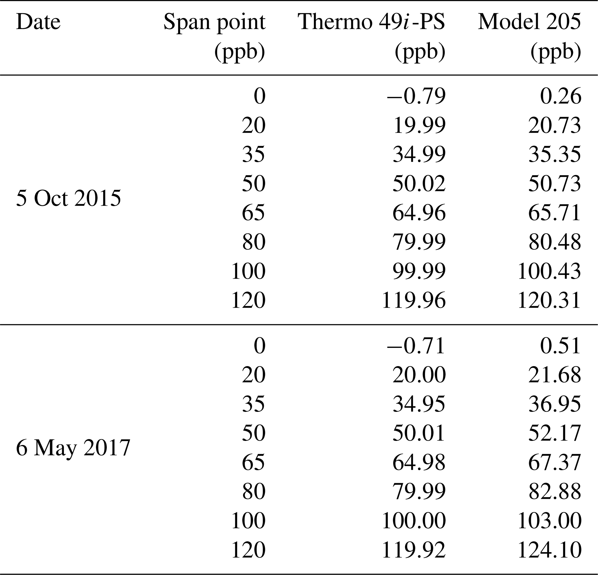
After the calibration of the internal zero and span settings, a second stage of calibration was performed involving multi-point verification to check the response and stability of the analyzer. On 5 October 2015 (before the instrument was shipped) and 6 May 2017 (the day that the instrument was transported back from Antarctica), a zero and seven upscale points (0, 20, 35, 50, 65, 80, 100, 120 ppb), encompassing the full scale of the observation range (Table 1), were generated by the Thermo 49i-PS to test the Model 205 analyzer. Each point was observed for 15 min, during the last 10 min of which readings of the calibrator and analyzer were taken every minute. Based on this experiment, the slope and intercept of the calibration curve were calculated by least squares. The results are shown in Table 2; it can be concluded that the slopes of the linear correction curve were 0.99936 and 1.02520, and the intercepts were 0.53861 and 0.85220l, which fulfilled the requirements of HJ 590-2010 and USEPA.
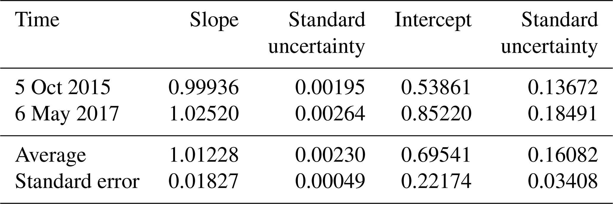
Another challenge when monitoring the atmosphere is the stability of the analyzer, which includes the analyzer's response time. Similarly to the regular calibration, its calibration could not be performed during the observation period, but it was reassuring that the Model 205 was still in good condition when we did the multi-point verification in May 2017, as shown in Table 2. The slope and intercept of the two calibration curves changed little, and the standard uncertainties were small. To further test the stability, data consistency was also examined, and the mean absolute deviation between two adjacent values was only 0.09 ppb. The largest difference was 0.61 ppb, indicating that the analyzer was stable and reliable.
Before analysis, a variance test was used to remove abnormal data based on the Laida criterion method, which assumes that the records obeyed a normal distribution. The formula is , where xi is the measured value, x is the time series mean and σ is the standard deviation. After processing, 99.3 %, 99.6 % and 89.3 % of the hourly mean data were retained from the Amundsen–Scott Station, Zhongshan Station and Kunlun Station, respectively.
2.3 Air mass back-trajectory calculations
Gridded meteorological data for backward trajectories in the Hybrid Single-Particle Lagrangian Integrated Trajectory (HYSPLIT) model were obtained from the Global Data Assimilation System (GDAS1) operated by NOAA with 1∘ ×1∘ horizontal resolution and 23 vertical levels, from 1000 to 20 hPa (http://www.arl.noaa.gov/gdas1.php, last access: 17 December 2020).
The HYSPLIT backward-trajectory air mass model was previously applied to atmospheric research in Antarctica (Legrand et al., 2009; Hara et al., 2011). We used the HYSPLIT model in this paper to analyze the impact of varying air mass sources and the intrusion of stratospheric O3. Backward trajectories and clusters were calculated using the NOAA HYSPLIT model (Draxler and Rolph, 2003; http://ready.arl.noaa.gov/HYSPLIT.php, last access: 17 December 2020), which is a free software plug-in for MeteoInfo (Wang, 2014; http://meteothink.org/, last access: 17 December 2020). The backward trajectories' starting height was set at 20 m above the surface; the total run time was 120 h for each backward trajectory, and each run was performed in time intervals of 6 h (00:00, 06:00, 12:00, 18:00 UTC).
The integral error part of the trajectory calculation error can be estimated by simulating the backward trajectory at the end of the forward trajectory and comparing the differences in the tracks. The starting point of the backward integration is set as (80.42∘ S, 77.12∘ E; 20 m a.g.l.); the backward integration is 120 h. Then the point reached at this time is taken as the starting point, and a forward simulation is made for 120 h. In this simulation experiment, the contribution of integration error to trajectory calculation error is very small within the first 72 h. With the extension of integration time, the integration error slightly increases.
The air mass trajectories were assigned to distinct clusters according to their moving speed and direction using a k-means clustering algorithm (Wong, 1979). As this study focused on the transport pathway of O3, the clustering result with the smallest number was selected as done by Wang (2014). It was found that three clusters perform best to represent the meteorological characteristics of the transport pathways at DA. This number was then selected as the expected number of air mass trajectory clusters. A more detailed clustering procedure using the k-means algorithm can be found in Wang (2014).
2.4 Potential source contribution function
The observation of a secondary maximum of O3 in November–December at the inland Antarctic sites was first reported for SP by Crawford et al. (2001) and was attributed to photochemical production induced by high NOx levels in the atmospheric surface layer, which were generated by the photodenitrification of the Antarctic snowpack (same as Davis et al., 2001). At Dome C (DC), a secondary maximum in November–December 2007 was also reported by Legrand et al. (2009), proving that photochemical production of O3 in the summer takes place over a large part of the Antarctic Plateau. A further study by Legrand et al. (2016) found that the highest near-surface O3 summer values were observed within air masses that spent extensive time over the highest part of the Antarctic Plateau before arriving at DC. To investigate the possible influence of synoptic-scale air mass circulation on the occurrence of OEEs at DA, 5 d HYSPLIT back-trajectories were analyzed (Fig. 9). We used the potential source contribution function (PSCF; see, e.g., Hopke et al., 1995; Brattich et al., 2017) to calculate the conditional probabilities and identify the geographical regions related to the occurrence of no-O3 enhancement events (NOEEs) and OEEs at DA (Fig. 7).
As in Yin et al. (2017), the potential source contribution function (PSCF) assumes that back trajectories arriving at times of high concentrations likely point to significant pollution directions (Ashbaugh et al., 1985). This function was often applied to locate air masses associated with high levels of near-surface O3 at different sites (Kaiser et al., 2007; Dimitriou and Kassomenos, 2015). In this study, the PSCF was calculated using HYSPLIT trajectories. The top of the model was set to 10 000 m a.s.l. The PSCF values for the grid cells in the study domain were calculated by counting the trajectory segment endpoints that terminated within each cell (Ashbaugh et al., 1985). If the total number of endpoints that fall in a cell is nij and there are mij points for which the measured O3 parameter exceeds a criterion value selected for this parameter, then the conditional probability, the PSCF, can be determined as
The concentrations of a given analyte greater than the criterion level are related to the passage of air parcels through the ijth cell during transport to the receptor site. That is, cells with high PSCF values are associated with the arrival of air parcels at the receptor site, which has near-surface O3 concentrations that are higher than the criterion value. These cells are indicative of areas with “high potential” contributions of the constituent. Identical PSCFij values can be obtained from cells with very different counts of back-trajectory points (e.g., grid cell A with mij=5000 and nij=10 000 and grid cell B with mij=5 and nij=10). In this extreme situation, grid cell A has 1000 times more air parcels passing through it than grid cell B. Because the particle count in grid cell B is sparse, the PSCF values in this cell are highly uncertain. To explain the uncertainty due to the low values of nij, the PSCF values were scaled by a weighting function Wij (Polissar et al., 1999). The weighting function reduced the PSCF values when the total number of endpoints in a cell was less than approximately 3 times the average number of endpoints per cell. In this case, Wij was set as follows:
where Nave represents the mean nij of all grid cells. The weighted PSCF values were obtained by multiplying the original PSCF values by the weighting factor.
3.1 Mean concentration
At the DA, SP and ZS sites, the annual mean concentrations of near-surface O3 were 29.2±7.5 ppb, 29.9±5.0 ppb and 24.1±5.8 ppb, respectively; the maximum annual mean concentration reached 42.5, 46.4 and 32.8 ppb, respectively; and the minimum annual mean concentrations were 14.0, 10.9 and 9.9 ppb, respectively. The inland stations are characterized by higher annual mean concentrations than the coastal station.
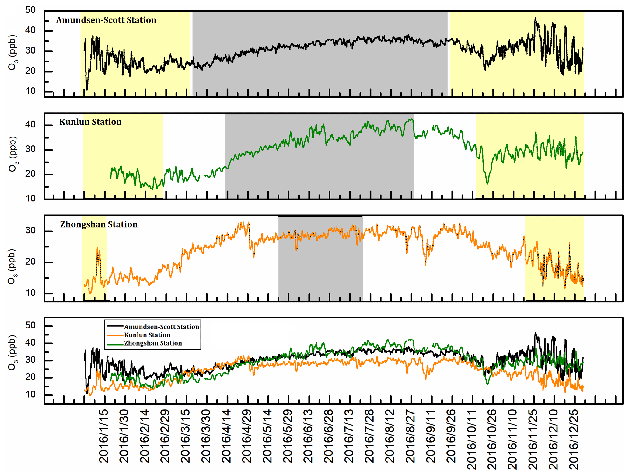
Figure 2Time series of near-surface O3 at SP, DA and ZS during 2016. Yellow (gray) shading identifies the polar day (night).
There were also obvious differences between the polar day and the polar night at all stations. In Fig. 2, we define the polar-day and polar-night windows by the day of year margins and have used different color shading to identify the polar day and polar night. The average concentrations of near-surface O3 during the polar night at the DA, SP and ZS sites were 34.1±4.3, 31.5±3.9 and 28.7±1.3 ppb, respectively, and much lower concentrations appeared during the non-polar night, with corresponding values of 26.1±7.0, 28.1±5.8 and 23.1±5.9 ppb, respectively. Interestingly, SP had the highest near-surface O3 concentration during the non-polar night, whereas at DA the highest concentration occurred during the polar night, and the largest variation also occurred at this site.
3.2 Seasonal variation
In this part, we define October–March as the warm season and April–September as the cold season, which is similar to the definition of polar day and night.
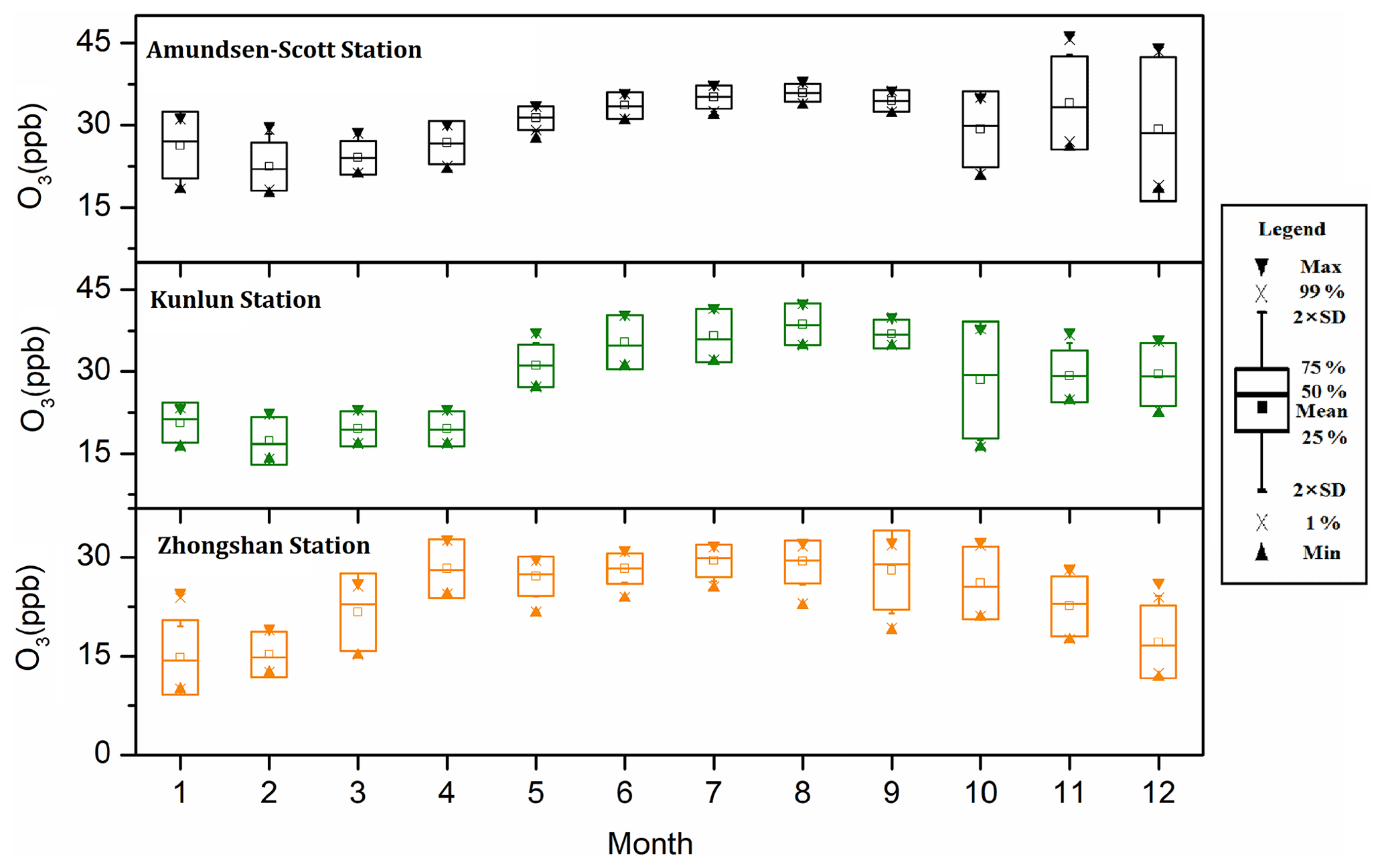
Figure 3Monthly average and statistical parameters of near-surface O3 at SP, DA and ZS during 2016.
In agreement with previous studies (Oltmans and Komhyr, 1976; Gruzdev et al., 1993; Ghude et al., 2005), the concentrations of near-surface O3 at the three stations were high and less variable during the cold season and low and more variable during the warm season (Fig. 3). In Antarctica, the emissions of O3 precursors are generally less than those at middle and low latitudes, whereas ultraviolet radiation is relatively strong; thus, when solar radiation occurs, the depletion effect is much greater than the effects from photochemical reactions during the warm season (Schnell et al., 1991). As explained by previous studies, during the polar night, due to the lack of light, the photochemical reactions stopped. Moreover, due to the lack of loss effect, the O3 concentration gradually increased and the fluctuations became smaller. During the polar night, the monthly variation in surface O3 at ZS was lower than that at DA but higher than that at SP. However, due to strong UV radiation in the low-latitude areas and the presence of bromine-controlled O3 depletion events in coastal areas, ZS shows large seasonal variations during the non-polar night (Wang et al., 2011; Prados-Roman et al., 2017). However, at SP, the largest standard deviation was observed in December, similarly to the characteristics at Dome C station (DC) from November to December (Legrand et al., 2009; Cristofanelli et al., 2018). Figures 2 and 3 indicate that the near-surface O3 showed obviously larger variations at DA than at SP during the polar night, since, due to the different geographical location, the meteorological conditions of DA and SP are different. The abnormal fluctuation in O3 concentration over DA during the polar night may be related to its special geographical environment.
As mentioned in the introduction section, mountainous topography and mountain waves may disturb advection transport in the stratosphere and lead to downward transportation to the troposphere (Robinson et al., 1983). DA is on the summit of the East Antarctic Ice Sheet, and the tropospheric depth is only ∼4.6 km (Liang et al., 2015), which favors exchange between the stratosphere and troposphere. However, the topography in this area is very flat and creates a disadvantage for mountain waves. Does O3 transport occur? We will analyze and discuss this question in Sect. 4.

Figure 4Mean diurnal variations in near-surface O3 concentrations at SP (a), DA (b) and ZS (c) during 2016.
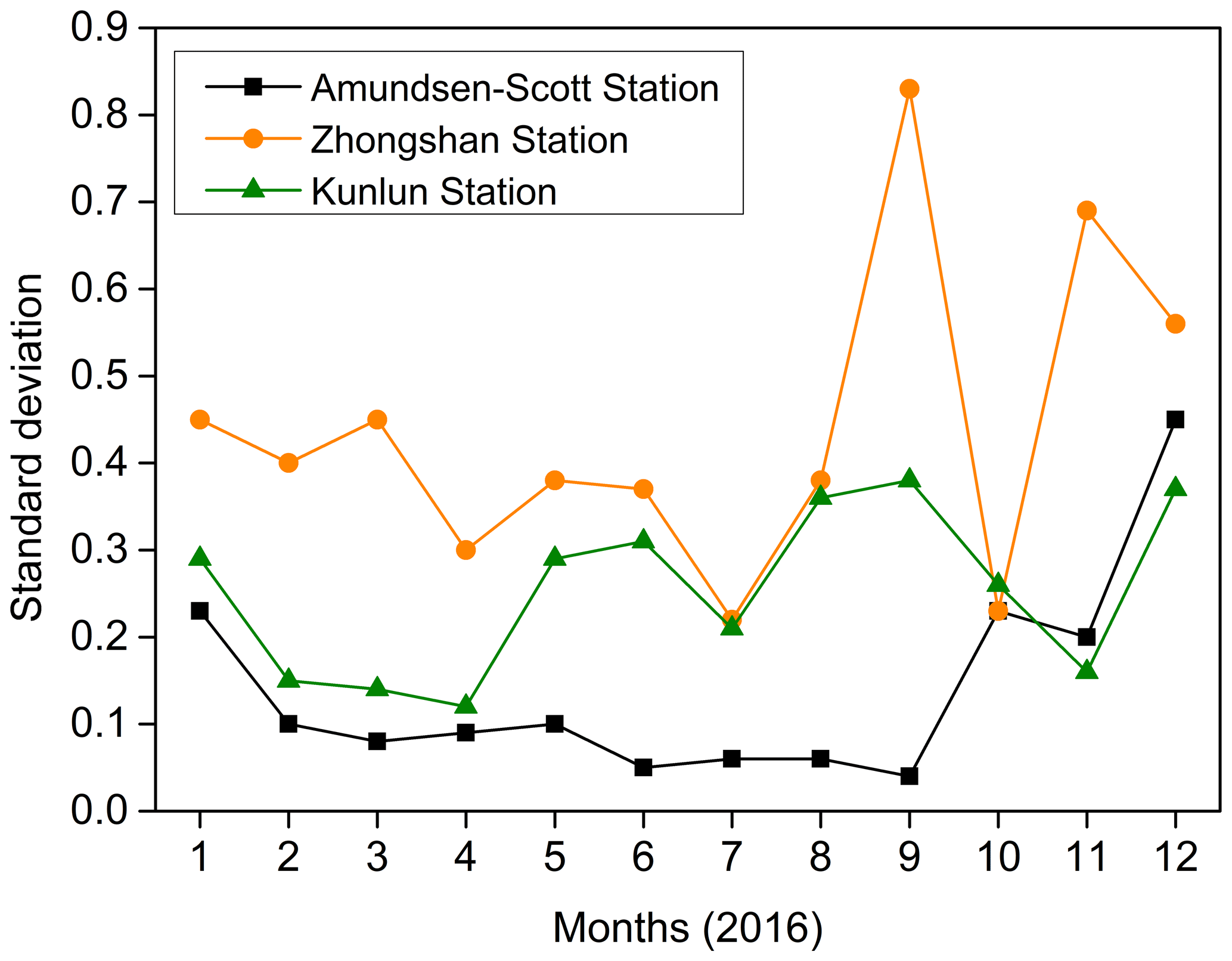
Figure 5Standard deviations of mean diurnal variation in near-surface O3 concentrations at SP, DA and ZS during 2016.
3.3 Diurnal variation
To characterize the typical monthly O3 diurnal variations at the three stations, we analyzed the mean diurnal variations in O3 at the three stations (Fig. 4) and the standard deviation of the mean diurnal variations (Fig. 5). At the DA site, the mean diurnal concentrations for each month were relatively steady, with the standard deviation of the mean diurnal concentration for each month being lower than 0.4 ppb. At SP, the mean diurnal concentrations were less variable as well. Except for December, the standard deviation of the mean diurnal concentration was lower than 0.3 ppb. At ZS, except for October, the standard deviation of the mean diurnal concentration was greater than that at the other two stations. In particular, the standard deviation of the mean diurnal concentration of ZS in September, November and December exceeded 0.5 ppb. Obviously, the average daily concentration fluctuation in Zhongshan Station was obviously different with the two inland stations, which can be attributed to their background climates. In spring, ozone depletion events (ODEs) occur frequently at Zhongshan Station. And this phenomenon is always accompanied by abrupt weather transition from continental dominant to oceanic dominant; in other words, the BrO brought by northerly wind from sea ice areas could lead to serious ozone depletion (Wang et al., 2011; Ye et al., 2017). In contrast, at inland stations like DA and SP, there were rarely ODEs.
On the whole, the mean diurnal variations in different time periods were not obvious, and the mean diurnal concentrations of the three stations fluctuated within a range of less than 1 ppb. The magnitude of the diurnal variation was low, which is similar to the variations in other Antarctic stations, Neumayer and Marambio for instance (Nadzir et al., 2018).
4.1 Identification of OEEs
Our method to select the days characterized by OEEs is based on the procedure used in Cristofanelli et al. (2018). First, a sinusoidal fit is used to calculate the O3 annual cycle not affected by the OEEs; then a probability density function (PDF) of the deviations from the sinusoidal fit is calculated, with the application of a Gaussian fit to the obtained PDF. As reported in Giostra et al. (2011), the deviations from the Gaussian distribution (calculated by using the Origin® 9 statistical tool) can be used to identify observations affected by non-background variability. We computed the further Gaussian fitting of PDF points beyond 1σ (standard deviation) of the Gaussian PDF and determined the non-background O3 daily values that may be affected by “anomalous” O3 enhancement. The intersection of the two fitting curves is taken as our screening threshold (3.4 ppb at SP, 3.4 ppb at DA and 2.5 ppb at ZS). Figure 6a, b and c show OEE days and NOEE days at these three stations, while Fig. 6d, e and f report the distribution frequency of OEE days.
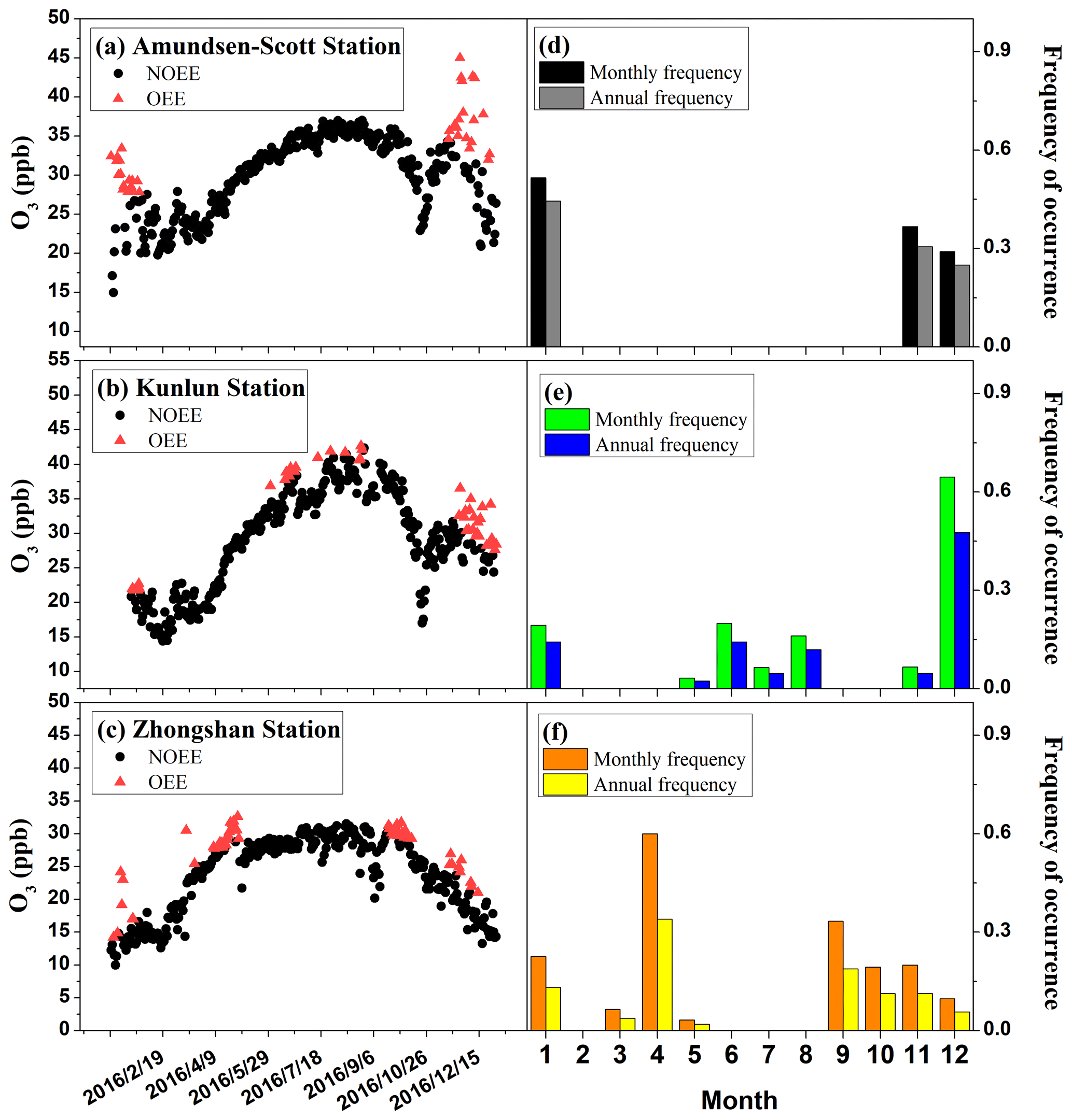
Figure 6(a–c) The OEEs and (d–f) averaged distribution of OEE occurrence among the different months of 2016 at the three stations. ; .
In total, 42 d at DA were found to be affected by anomalous OEEs: 14.3 % in January, 2.4 % in May, 14.3 % in June, 4.8 % in July, 11.9 % in August, 4.8 % in November and 47.6 % in December (Fig. 6e, blue bars). This result clearly indicates that half of the anomalous days occurred in December, followed by January and June. At SP, 36 d with OEEs were found in 2016: 44.4 % in January, 30.6 % in November and 25 % in December (Fig. 6d, gray bars). Apparently, OEEs occur only in summertime at this measurement site. ZS was characterized by more days with OEEs: 53 d in April (34.0 %), followed by September (18.9 %), January (13.2 %), October (11.3 %), November (11.3 %), December (5.7 %) March (3.8 %) and May (1.9 %) (Fig. 6f, yellow bars).
From the results above, it can be seen that SP was characterized by concentrated OEE occurrences, and ZS had the most scattered OEEs pattern. In addition, all OEEs at SP and ZS occurred during the Antarctic warm season, and no OEEs were present during the polar night, similarly to the pattern observed at DC (Cristofanelli et al., 2018). In contrast, the OEEs also occurred during the polar night at DA, and the number of OEE occurrence days accounted for up to 33 % of the total number of events throughout the year. This is the main reason for the large variations in daily average concentration during the polar night at DA.
Previous studies (e.g., Legrand et al., 2016; Cristofanelli et al., 2018) carried out in DC showed that the O3 variability at DC could be associated with processes occurring at long temporal scales. In addition, the accumulation of photochemically produced O3 during transport of air masses was the main reason for OEEs, whereas the stratospheric intrusion events had only a minor influence on OEEs (up to 3 %). This finding cannot explain the temporal occurrence pattern of OEEs at DA. To determine the unknown cause, we investigated the synoptic-scale air mass transport and the STT occurrence at the measurement site.
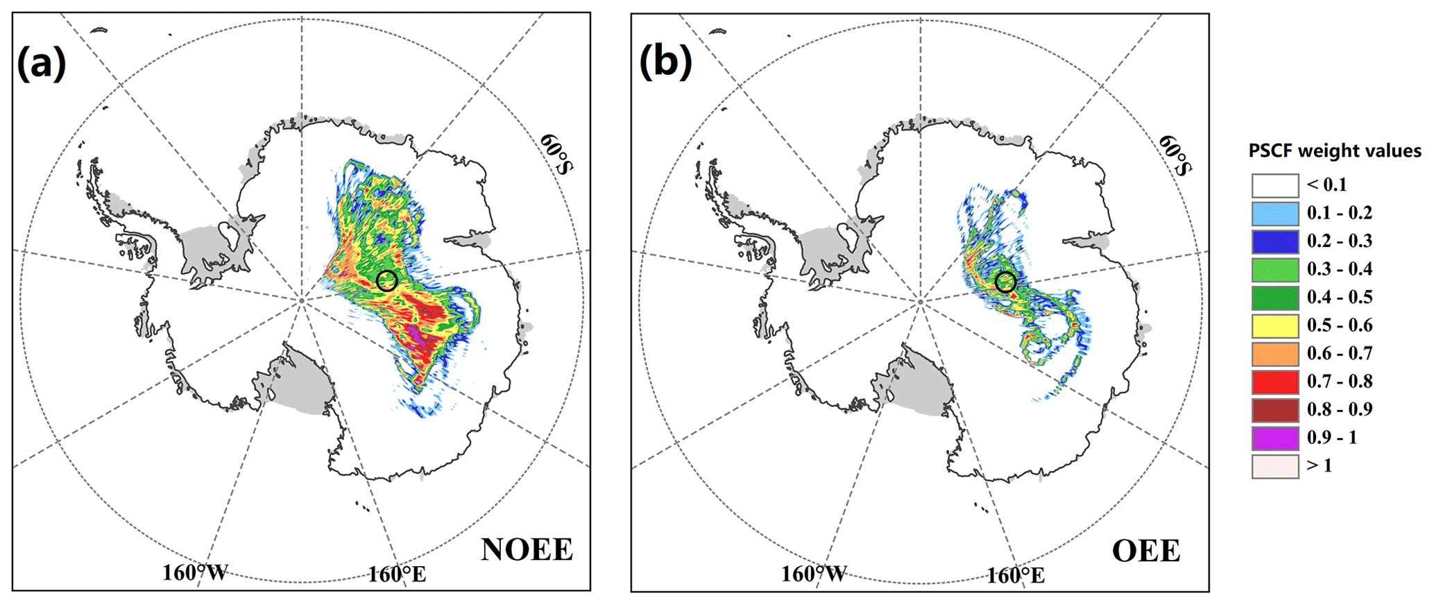
Figure 7Likely source areas of surface O3 at Kunlun Station during the NOEE (a) and OEE (b) identified using the PSCF (potential source contribution function).
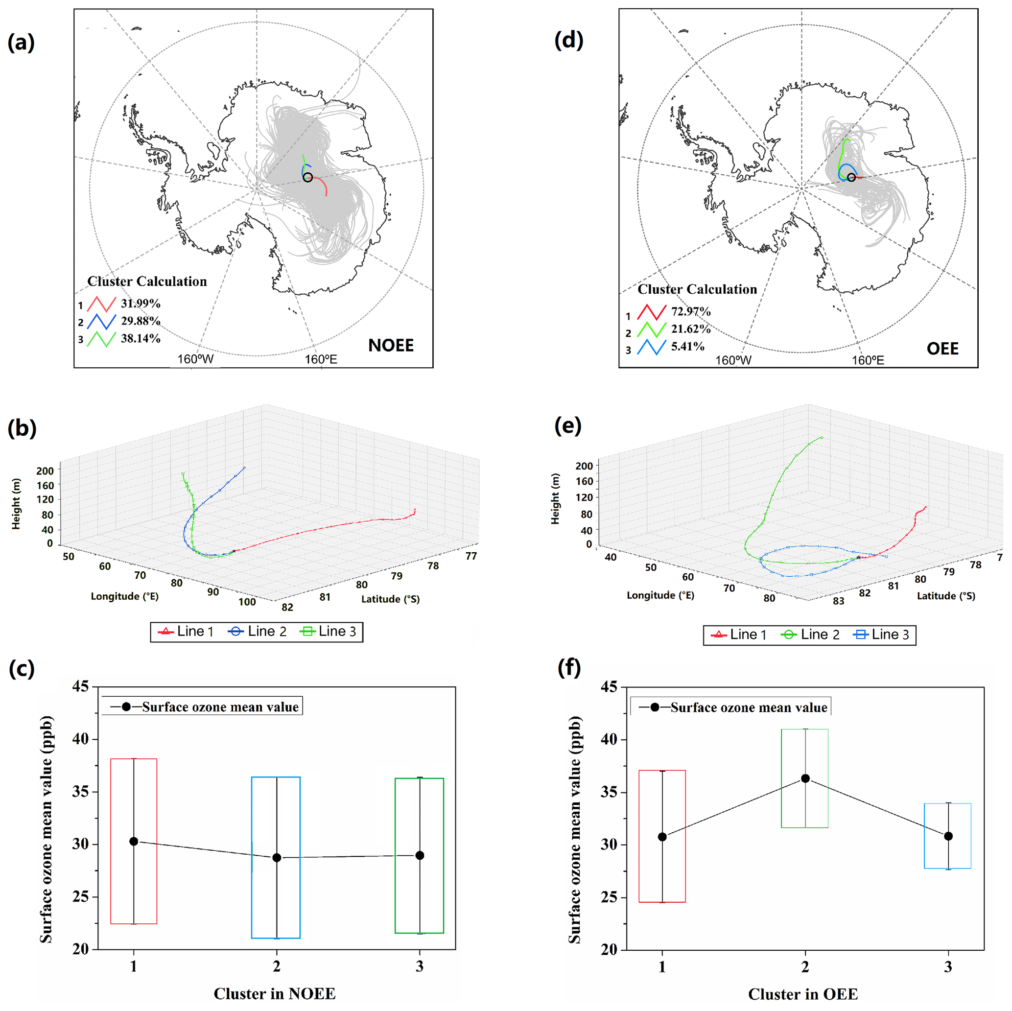
Figure 8Backward HYSPLIT trajectories for each measurement day (gray lines in panel a) and mean back trajectory for three HYSPLIT clusters (colored lines in panel a; 3-D view shown in panel b) arriving at Kunlun Station during NOEEs. Panel (c) shows the range of surface ozone concentrations measured at DA by cluster. The error bar is the standard deviation of the same cluster. Panels (d)–(f) are the same as panels (a)–(c) but for OEEs.
4.2 Role of synoptic-scale air mass transport
During NOEEs, the air masses arriving at DA mainly come from the west and east of DA, and the 3-D clusters show that the air masses traveled over the Antarctic Plateau before reaching DA (Fig. 8b). The difference in the number of the three cluster trajectories is small, and the difference in the corresponding cluster average concentrations is not large. Using the PSCF results, we have identified air masses associated with higher surface ozone at DA during NOEEs (Fig. 8a). The Antarctic Plateau to the east and west of DA had high PSCF weight values (Fig. 7), which shows that, during NOEEs, the potential source area of surface O3 for DA is mainly in the inland plateaus in the east and west, and the area of high-PSCF-weight-value distribution in the east is larger than in other directions.
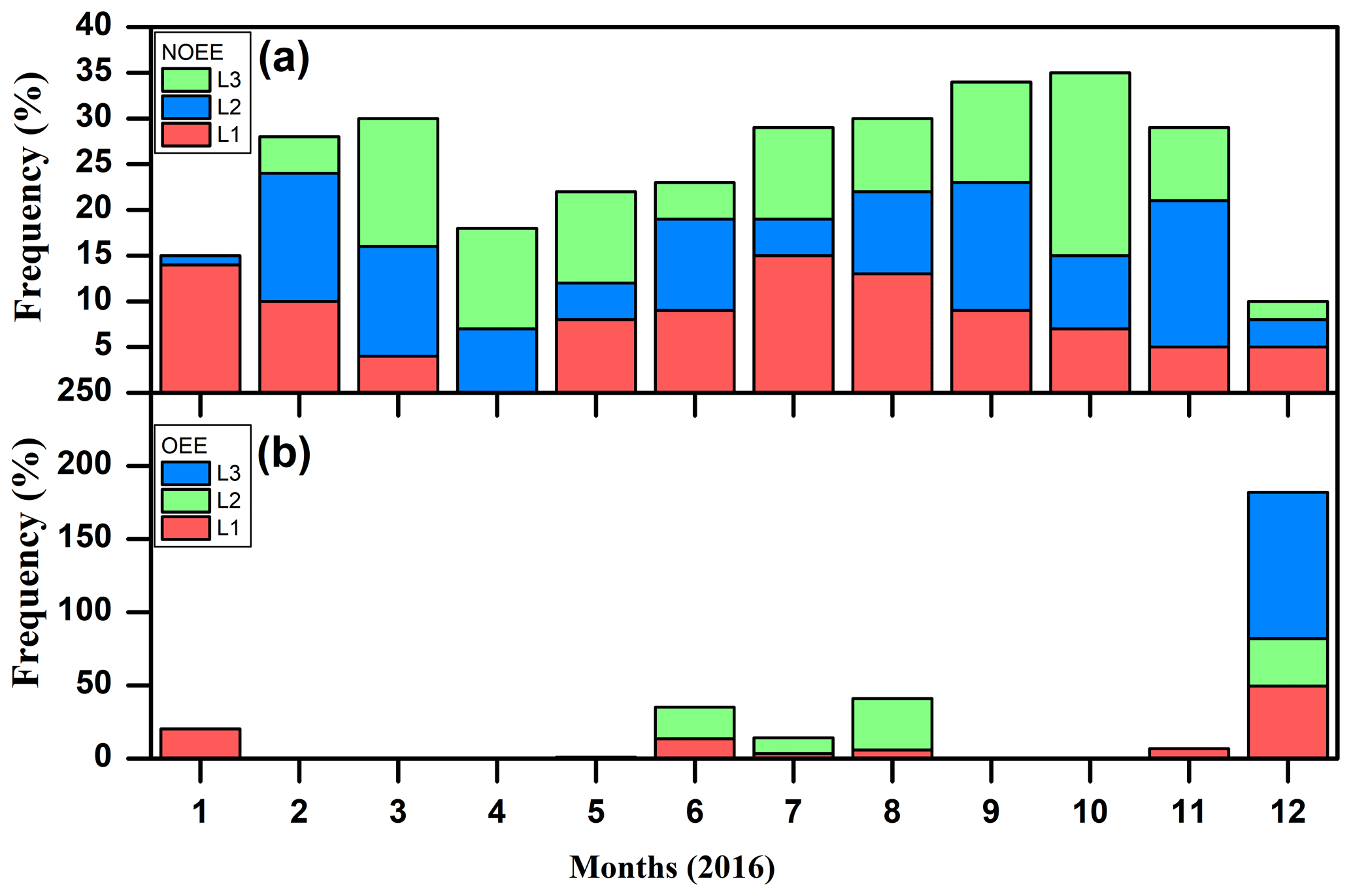
Figure 9Monthly frequency distribution of clustering trajectories (Line 1, 2, 3) during NOEEs and OEEs.
Compared with NOEEs, the clustering results of trajectories during OEEs have different characteristics. In OEEs, the air masses that arrived at DA were prevalent from the north and from the west, and the 3-D clusters indicated that 73 % of the air mass trajectories came from the area north of DA (red line in Fig. 8e). The average concentrations of the three clusters differ greatly (Fig. 8f), but they are all higher than those obtained for NOEEs. It should be noted that 68 % of Line-2 cluster (green line in Fig. 8d) occurred during the polar night (Fig. 9) and had a high average O3 concentration (reached 36.3 ppb). This shows that the OEEs of the polar night are more affected by the high-value O3 air masses over the plateau west of DA than those during the polar day. Using the PSCF results, during OEEs, we did not find a large area of high WPSCF values; the high WPSCF value only appeared in the east and the north of DA over a limited area. However, independently of the polar day or of the polar night, the Line-1 cluster trajectory accounted for more than 60 % during OEEs. In addition, the short distance of the Line-1 cluster trajectory indicates that the air mass transport speed is slow, which is conducive to the accumulation of O3 along the way. It can be seen from Fig. 8e that the characteristic values of backward-trajectory clustering during OEEs are mostly lower than 200 m a.g.l. (supporting the role of snow as the source of near-surface O3). As Fiebig et al. (2014) have proposed, the increase in O3 values in the near surface of central Antarctica may also be related to the transport of free tropospheric air and aged pollution plumes from low latitudes. In addition, Fig. 10 shows that the average O3 growth rate reached 0.29 ppb h−1 during OEEs in the polar night, while the average O3 growth rate was −0.06 ppb h−1 during NOEEs in the polar night (Fig. 10). The statistical scatter distribution showed that 97 % of OEEs occurred when the wind speed was lower than 4 m s−1. The overall average wind speed during OEEs is also significantly lower than that of NOEEs. As Helmig et al. (2008a) have proposed, during stable atmospheric conditions (which typically existed during low-wind and fair-sky conditions) ozone accumulates in the surface layer, and its concentration increases rapidly.
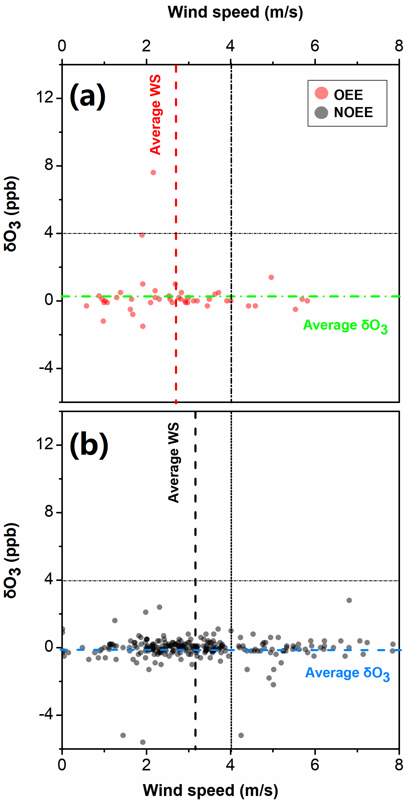
Figure 10Wind speed and ΔO3 statistical distribution around OEEs (red dots) and NOEEs (black dots) at DA in the polar night. Here, ΔO3 represents the growth rate of near-surface O3 concentration, calculated by the following equation: .
This finding confirms that the OEEs of DA are mainly caused by the accumulation of high concentrations of air masses transported nearby, and the synoptic-scale transport can favor the photochemical production and the accumulation of O3 accumulation by air masses traveling over the plateau near the north of DA before their arrival.
4.3 Role of STT events
4.3.1 Identification of deep STT events
Several methods can be applied to study stratosphere-to-troposphere transport (STT) events. One method is the chemistry–climate hindcast model GFDL AM3, which Lin et al. (2017) used to evaluate the increasing anthropogenic emissions in Asia and Xu et al. (2018) used to examine the impact of direct tropospheric ozone transport at Waliguan Station. Stratosphere-to-Troposphere Exchange Flux (STEFLUX; Putero et al., 2016) is a novel tool to quickly obtain reliable identification of STT events occurring at a specific location and during a specified time window. STEFLUX relies on a compiled stratosphere-to-troposphere exchange climatology, making use of the ERA-Interim reanalysis dataset from the ECMWF and a refined version of a well-established Lagrangian methodology. STEFLUX is able to detect stratospheric intrusion events on a regional scale, and it has the advantage of retaining additional information concerning the pathway of stratosphere-affected air masses, such as the location of tropopause crossing and other meteorological parameters along the trajectories.
We applied STEFLUX to assess the possible contribution of STT to near-surface O3 variability in the DA region (i.e., STEFLUX “target box”; for further details on the methodology see Putero et al., 2016), and to identify the measurement periods possibly affected by “deep” STT events (i.e., stratospheric air masses transferred down to the lower troposphere). For this work, we set the top lid of the box at 500 hPa and the following geographical boundaries: 79–82∘ S, 76–79∘ E. A deep STT event at Kunlun Station was determined if at least one stratospheric trajectory crossed the 3-D target box.
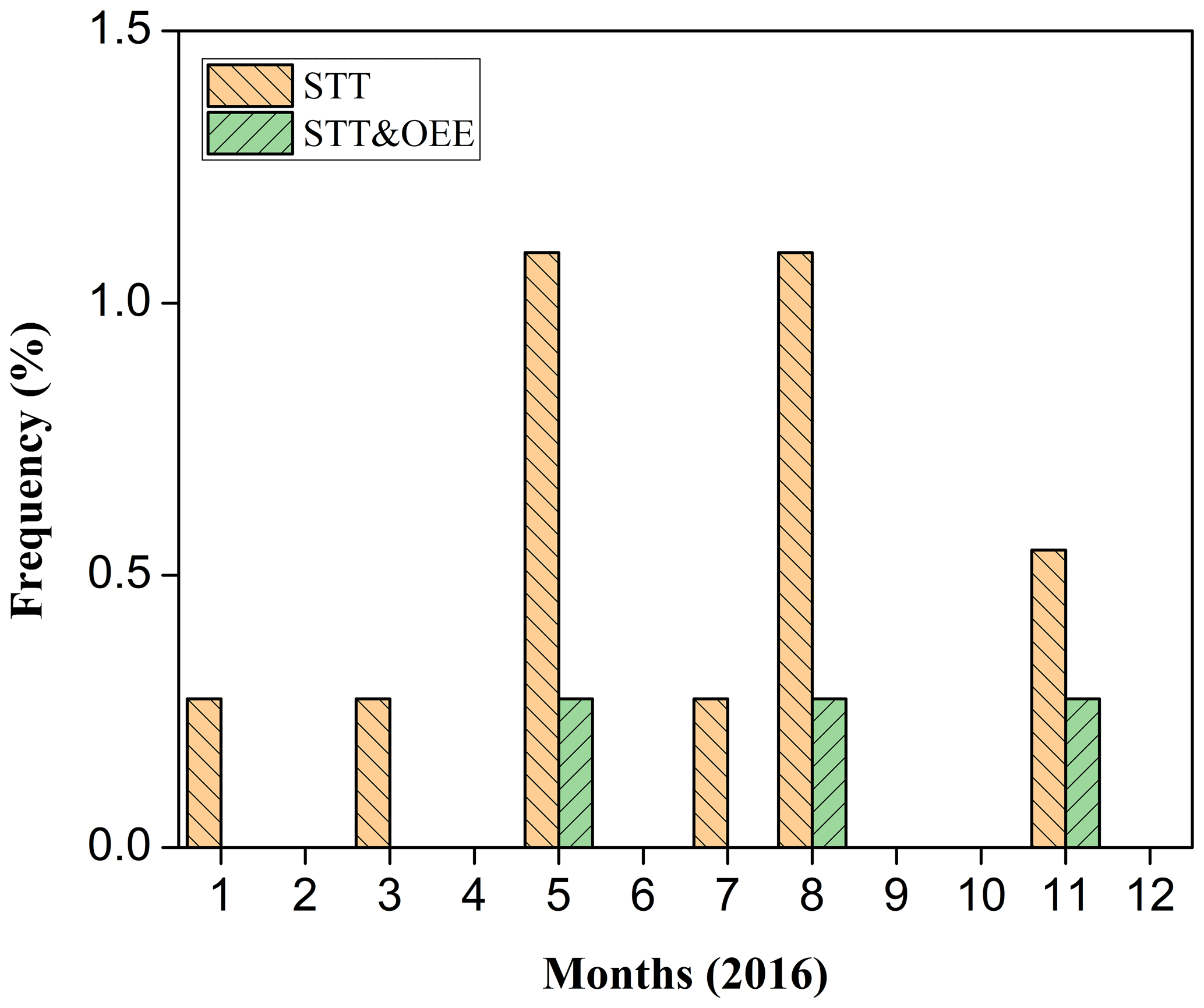
Figure 11Annual variation in deep STT events at Kunlun Station and the annual variation in it that occurred at the same time as OEEs over the period 2016, obtained by STEFLUX.
4.3.2 Role of STT events at DA
The possible occurrence of stratospheric intrusion events and their role in affecting the variability in near-surface O3 and tropospheric air chemistry in Antarctica has been investigated in several studies (Murayama et al., 1992; Roscoe, 2004; Stohl and Sodemann, 2010; Mihalikova and Kirkwood, 2013; Traversi et al., 2014, 2017; Cristofanelli et al., 2018). To provide a systematic assessment of the possible influence of deep STT events on the near-surface O3 variability at Kunlun Station, we used the STEFLUX tool (see Sect. 4.3.1). Figure 11 shows the distribution of the occurrence of deep STT events over DA during the year. Although it is difficult to see a clear seasonal cycle due to the low frequency of deep STT events, our results are in agreement with previous studies, indicating STT influence of up to 2 % on a monthly basis (Stohl and Sodemann, 2010; Cristofanelli et al., 2018). According to our STEFLUX outputs, the highest frequency of deep STT events was observed in May and August (1.1 %). The frequency of occurrence of deep STT events identified by STEFLUX at Kunlun Station is about 1 order of magnitude lower than the occurrence of OEEs. Thus, a direct link of STT with OEE interannual variability is unlikely, as also reported for the DC station (Cristofanelli et al., 2018). Nevertheless, STT events can be a source of nitrates for the Antarctic atmosphere through different processes, thus indirectly affecting near-surface O3 concentrations and favoring the presence of OEEs (Traversi et al., 2014, 2017).
All data presented in this paper are available at https://doi.org/10.5281/zenodo.3923517 (Ding and Tian, 2020). The dataset covers the hourly average concentrations of near-surface ozone at three stations (i.e., SP, ZS, DA).
Based on the in situ monitoring data during 2016 at DA, the variation, formation and decay mechanisms of near-surface O3 were studied and compared with those at SP and ZS. The annual mean concentrations of near-surface O3 at the DA, SP and ZS sites were 29.2±7.5, 29.9±5.0 and 24.1±5.8 ppb, respectively. The near-surface O3 concentrations were clearly higher in the winter polar night, with small fluctuations, than in the other seasons, which is different from the patterns observed at low latitudes. The O3 over inland areas was also higher than over the coast.
The diurnal variations showed nonsignificant regular patterns, and the range of the average diurnal concentration fluctuation was less than 1 ppb at all three stations. These findings suggest that the synoptic transport somehow controls the overall O3 variability, as has been shown at SP and DC (Neff et al., 2008b; Cristofanelli et al., 2018).
At Kunlun Station, it is unlikely that there is a direct relationship between STT and OEEs. The frequency of deep STT events identified by STEFLUX is about an order of magnitude lower than OEEs and reaches its highest frequency (1.1 %) in May and August. As deduced by the STEFLUX application, deep STT events play a marginal role in steering the occurrence of OEEs at DA via “direct” transport of O3 from the stratosphere or the free troposphere to the surface. As explained in Cristofanelli et al. (2018), this can be related to an underestimation of “young” (i.e., <4 d old) STT events by STEFLUX or to an insufficient spatial and vertical resolution from ERA-Interim to fully resolve the complex STT in the Antarctic atmosphere (Mihalikova and Kirkwood, 2013). Despite this, STT can still represent a source of nitrates for the Antarctic snowpack, thus possibly affecting summer photochemical O3 production. Therefore, it is important to carry out further studies to better assess these processes.
The characteristics and mechanisms of near-surface O3 revealed in this paper have important implications for better understanding the formation and decay processes of near-surface O3 in Antarctica, especially over the plateau areas. Nevertheless, the lack of observations restricted our ability to amass more information. Long-term sustained observations at Dome A, Dome C, Dome F, SP, Vostok and other locations would greatly help in the future.
The supplement related to this article is available online at: https://doi.org/10.5194/essd-12-3529-2020-supplement.
MD and BT designed the experiments and wrote the manuscript; MD carried out the experiments; BT analyzed the experimental results. MD, BT and DP revised the manuscript; DP run the STEFLUX tool. MCBA, ZZ, LW, SY, JT, CL and CX discussed the results.
The authors declare that they have no conflict of interest.
This work is financially supported by the National Natural Science Foundation of China (41771064), the Strategic Priority Research Program of Chinese Academy of Sciences (XDA20100300) and the Basic Fund of the Chinese Academy of Meteorological Sciences (2018Z001 and 2019Y010). The observations were carried out by during the Chinese National Antarctic Research Expedition at Zhongshan Station and Kunlun Station. We are also grateful to NOAA for providing the HYSPLIT model and GFS meteorological files. Yaqiang Wang is the developer of MeteoInfo and provided generous help for the paper. PLATO-A was supported by the Australian Antarctic Division and with NCRIS funding through Astronomy Australia Limited.
This research has been supported by the National Natural Science Foundation of China (grant no. 41771064), the Strategic Priority Research Program of the Chinese Academy of Sciences (grant no. XDA20100300) and the Basic Fund of the Chinese Academy of Meteorological Sciences (grant nos. 2018Z001 and 2019Y010).
This paper was edited by Alexander Kokhanovsky and reviewed by two anonymous referees.
Ashbaugh, L. L., Malm, W. C., and Sadeh, W. Z.: A residence time probability analysis of sulfur concentrations at Grand Canyon National Park, Atmos. Environ., 19, 1263–1270, https://doi.org/10.1016/0004-6981(85)90256-2, 1985.
Bauguitte, S. J.-B., Brough, N., Frey, M. M., Jones, A. E., Maxfield, D. J., Roscoe, H. K., Rose, M. C., and Wolff, E. W.: A network of autonomous surface ozone monitors in Antarctica: technical description and first results, Atmos. Meas. Tech., 4, 645–658, https://doi.org/10.5194/amt-4-645-2011, 2011.
Berman, S., Ku, J. Y., and Rao, S. T.: Spatial and Temporal Variation in the Mixing Depth over the Northeastern United States during the Summer of 1995, J. Appl. Meteorol., 38, 1661–1673, https://doi.org/10.1175/1520-0450(1999)038<1661:SATVIT>2.0.CO;2, 1999.
Brattich, E., Orza, J. A. G., Cristofanelli, P., Bonasoni, P., and Tositti, L.: Influence of stratospheric air masses on radiotracers and ozone over the central Mediterranean, J. Geophys. Res.-Atmos., 122, 7164–7182, https://doi.org/10.1002/2017JD027036, 2017.
Crawford, J. H., Davis, D. D., Chen, G., Buhr, M., Oltmans, S., Weller, R., Mauldin, L., Eisele, F., Shetter, R., Lefer, B., Arimoto, R., and Hogan, A.: Evidence for photochemical production of ozone at the South Pole surface, Geophys. Res. Lett., 28, 3641–3644, https://doi.org/10.1029/2001gl013055, 2001.
Cristofanelli, P., Bonasoni, P., Calzolari, F., Bonafè, U., Lanconelli, C., Lupi, A., Trivellone, G., Vitale, V., and Petkov, B.: Analysis of near-surface ozone variations in terra nova bay, Antarctica, Antarct. Sci., 20, 415–421, https://doi.org/10.1017/S0954102008001028, 2008.
Cristofanelli, P., Putero, D., Bonasoni, P., Busetto, M., Calzolari, F., Camporeale, G., Paolo, C., Giuseppe, L., Angelo, P., Boyan, T., Rita, U., and Roberto, V.: Analysis of multi-year near-surface ozone observations at the wmo/gaw “concordia” station (75∘06′s, 123∘20′e, 3280 m a.s.l. – antarctica), Atmos. Environ., 177, 54–63, https://doi.org/10.1016/j.atmosenv.2018.01.007, 2018.
Davidson, A.: Update on ozone trend in California's south coast air basin, J. Air Waste Manag. Assoc., 43, 226–227, https://doi.org/10.1080/1073161x.1993.10467130, 1993.
Davis, D. D., Nowak, L. B., Chen, G., Buhr, M., Arimoto, R., Hogan, A., Eisele, F., Mauldin, L., Tanner, D., Shetter, R., Lefer, B., and McMurry, P.: Unexpected high levels of NO observed at South Pole, Geophys. Res. Lett., 28, 3625–3628, 2001.
Dimitriou, K. and Kassomenos, P.: Three year study of tropospheric ozone with back trajectories at a metropolitan and a medium scale urban area in Greece, Sci. Total Environ., 502, 493–501, https://doi.org/10.1016/j.scitotenv.2014.09.072, 2015.
Ding, M. and Tian, B.: The surface ozone observation data of Kunlun station in 2016 [Data set], Zenodo, https://doi.org/10.5281/zenodo.3923517, 2020.
Draxler, R. R. and Rolph, G. D.: HYSPLIT (HYbrid Single-Particle Lagrangian Integrated Trajectory) Model, NOAA Air Resour, Lab., Silver Spring, Md., available at: http://ready.arl.noaa.gov/HYSPLIT.php, last access: 16 December 2020), 2003.
Fiebig, M., Hirdman, D., Lunder, C. R., Ogren, J. A., Solberg, S., Stohl, A., and Thompson, R. L.: Annual cycle of Antarctic baseline aerosol: controlled by photooxidation-limited aerosol formation, Atmos. Chem. Phys., 14, 3083–3093, https://doi.org/10.5194/acp-14-3083-2014, 2014.
Fishman, J., Brackftt, V. G., and Fakhruzzaman, K.: Distribution of tropospheric ozone in the tropics from satellite and ozonesonde measurements, J. Atmos. Terr. Phys., 54, 589–597, 1992.
Frey, M. M., Roscoe, H. K., Kukui, A., Savarino, J., France, J. L., King, M. D., Legrand, M., and Preunkert, S.: Atmospheric nitrogen oxides (NO and NO2) at Dome C, East Antarctica, during the OPALE campaign, Atmos. Chem. Phys., 15, 7859–7875, https://doi.org/10.5194/acp-15-7859-2015, 2015.
Ghude, S. D., Kumar, A., Jain, S. L., Arya, B. C., and Bajaj, M. M.: Comparative study of the total ozone column over maitri, antarctica during 1997, 2002 and 2003, Int. J. Remote Sens., 26, 3413–3421, https://doi.org/10.1080/01431160500076434, 2005.
Giostra, U., Furlani, F., Arduini, J., Cava, D., Manning, A., ODoherty, S., Reimann, S., and Maione, M.: The determination of a “regional” atmospheric background mixing ratio for anthropogenic greenhouse gases: a comparison of two independent methods, Atmos. Environ., 45, 7396–7405, https://doi.org/10.1016/j.atmosenv.2011.06.076, 2011.
Greenslade, J. W., Alexander, S. P., Schofield, R., Fisher, J. A., and Klekociuk, A. K.: Stratospheric ozone intrusion events and their impacts on tropospheric ozone in the Southern Hemisphere, Atmos. Chem. Phys., 17, 10269–10290, https://doi.org/10.5194/acp-17-10269-2017, 2017.
Gruzdev, A. N. and Sitnov, S. A.: Tropospheric ozone annual variation and possible troposphere-stratosphere coupling in the arctic and antarctic as derived from ozone soundings at resolute and amundsen-scott stations, Tellus B, 45, 89–98, https://doi.org/10.1034/j.1600-0889.1993.t01-1-00001.x, 1993.
Hara, K., Osada, K., Nishita-Hara, C., and Yamanouchi, T.: Seasonal variations and vertical features of aerosol particles in the Antarctic troposphere, Atmos. Chem. Phys., 11, 5471–5484, https://doi.org/10.5194/acp-11-5471-2011, 2011.
Helmig, D., Johnson, B., Oltmans, S. J., Neff, W., and Eisele, F.: Elevated ozone in the boundary layer at south pole, Atmos. Environ., 42, 2788–2803, https://doi.org/10.1016/j.atmosenv.2006.12.032, 2008a.
Helmig, D., Johnson, B. J., Warshawsky, M., Morse, T., Neff, W. D., and Eisele, F.: Nitric oxide in the boundary-layer at south pole during the antarctic tropospheric chemistry investigation (antci), Atmos. Environ., 42, 2817–2830, https://doi.org/10.1016/j.atmosenv.2007.03.061, 2008b.
Honrath, R. E., Guo, S., Peterson, M. C., Dziobak, M. P., Dibb, J. E., and Arsenault, M. A.: Photochemical production of gas phase NOx from ice crystal , J. Geophys. Res.-Atmos., 105, 24183–24190, https://doi.org/10.1029/2000JD900361, 2000a.
Honrath, R. E., Peterson, M. C., Dziobak, M. P., Dibb, J. E., Arsenault, M. A., and Green, S. A.: Release of NOx from sunlight-irradiated midlatitude snow, Geophys. Res. Lett., 27, 2237–2240, https://doi.org/10.1029/1999GL011286, 2000b.
Hopke, P. K., Barrie, L. A., Li, S.-M., Cheng, M.-D., Li, C., and Xie, Y.: Possible sources and preferred pathways for biogenic and non-sea-salt sulfur for the high Arctic, J. Geophys. Res.-Atmos., 100, 16595–16603, https://doi.org/10.1029/95JD01712, 1995.
IPCC: Summary for policymakers [M], in: Climate Change 2013: The Phsical Science Basis, Contribution of Working Group to the fifth assessment report of the Intergovernmental Panel on Climate Change, Cambridge University Press, Cambridge, New York, 2013.
Johnson, T., Capel, J., and Ollison, W.: Measurement of microenvironmental ozone concentrations in Durham, North Carolina, using a 2B Technologies 205 Federal Equivalent Method monitor and an interference-free 2B Technologies 211 monitor, J. Air Waste Manag. Assoc., 64, 360–371, https://doi.org/10.1080/10962247.2013.839968, 2014.
Jones, A. E. and Wolff, E. W.: An analysis of the oxidation potential of the South Pole boundary layer and the influence of stratospheric ozone depletion, J. Geophys. Res., 108, 4565, https://doi.org/10.1029/2003JD003379, 2003.
Jones, A. E., Weller, R., Wolff, E. W., and Jacobi, H. W.: Speciation and rate of photochemical NO and NO2 production in Antarctic snow, Geophys. Res. Lett., 27, 345–348, https://doi.org/10.1029/1999GL010885, 2000.
Kaiser, A., Scheifinger, H., Spangl, W., Weiss, A., Gilge, S., Fricke, W., Ries, L., Cemas, D., and Jesenovec, B.: Transport of nitrogen oxides, carbon monoxide and ozone to the alpine global atmosphere watch stations Jungfraujoch (Switzerland), Zugspitze and Hohenpeißenberg (Germany), Sonnblick (Austria) and Mt.Krvavec (Slovenia), Atmos. Environ., 41, 9273–9287, https://doi.org/10.1016/j.atmosenv.2007.09.027, 2007.
Lawrence, J. S., Ashley, M. C. B., Hengst, S., Luong-Van, D. M., Storey, J. W. V., Yang, H., Zhou, X., and Zhu, Z.: The PLATO Dome A site testing observatory: power generation and control systems, Rev. Sci. Instr., 80, 064501-1–064501-10, 2009.
Legrand, M., Preunkert, S., Jourdain, B., Gallée, H., Goutail, F., Weller, R., and Savarino, J.: Year-round record of surface ozone at coastal (Dumont d'Urville) and inland (Concordia) stations in East Antarctica, J. Geophys. Res.-Atmos., 114, D20, https://doi.org/10.1029/2008JD011667, 2009.
Legrand, M., Preunkert, S., Savarino, J., Frey, M. M., Kukui, A., Helmig, D., Jourdain, B., Jones, A. E., Weller, R., Brough, N., and Gallée, H.: Inter-annual variability of surface ozone at coastal (Dumont d'Urville, 2004–2014) and inland (Concordia, 2007–2014) sites in East Antarctica, Atmos. Chem. Phys., 16, 8053–8069, https://doi.org/10.5194/acp-16-8053-2016, 2016.
Lei, B. and Min, L.: Discussion on Maintenance of O_342M type Automatic Ozone Analyzer, Environmental Science Survey, 33, 90–93, https://doi.org/10.3969/j.issn.1673-9655.2014.03.025, 2014.
Liang, F., Cunde, X., and Lingen, B.: Vertical Structure of Atmosphere on East Antarctic Plateau, Plateau Meteorology, 34, 299–306, https://doi.org/10.7522/j.issn.1000-0534.2014.00032, 2015.
Lin, C., Gillespie, J., Schuder, M. D., Duberstein, W., Beverland, I. J., and Heal, M. R.: Evaluation and calibration of aeroqual series 500 portable gas sensors for accurate measurement of ambient ozone and nitrogen dioxide, Atmos. Environ., 100, 111–116, https://doi.org/10.1016/j.atmosenv.2014.11.002, 2015.
Lin, M., Horowitz, L. W., Payton, R., Fiore, A. M., and Tonnesen, G.: US surface ozone trends and extremes from 1980 to 2014: quantifying the roles of rising Asian emissions, domestic controls, wildfires, and climate, Atmos. Chem. Phys., 17, 2943–2970, https://doi.org/10.5194/acp-17-2943-2017, 2017.
Liu, J., Zhang, X. L., Zhang, X. C., and Tang, J.: Surface Ozone Characteristics and the Correlated Factors at Shangdianzi Atmospheric Background Monitoring Station, Res. Environ. Sci., 19, 19–25, https://doi.org/10.1016/S1872-2040(06)60041-8, 2006.
Mickley, L. J., Murti, P. P., Jacob, D. J., Logan, J. A., Koch, D. M., and Rind, D.: Radiative forcing from tropospheric ozone calculated with a unified chemistry–climate model, J. Geophys. Res.-Atmos., 104, 30153–30172, https://doi.org/10.1029/1999JD900439, 1999.
Mihalikova, M. and Kirkwood, S.: Tropopause fold occurrence rates over the Antarctic station Troll (72∘ S, 2.5∘ E), Ann. Geophys., 31, 591–598, https://doi.org/10.5194/angeo-31-591-2013, 2013.
Monks, P. S., Archibald, A. T., Colette, A., Cooper, O., Coyle, M., Derwent, R., Fowler, D., Granier, C., Law, K. S., Mills, G. E., Stevenson, D. S., Tarasova, O., Thouret, V., von Schneidemesser, E., Sommariva, R., Wild, O., and Williams, M. L.: Tropospheric ozone and its precursors from the urban to the global scale from air quality to short-lived climate forcer, Atmos. Chem. Phys., 15, 8889–8973, https://doi.org/10.5194/acp-15-8889-2015, 2015.
Moura, B. B., de Souza, S. R., and Alves, E. S.: Respostas estruturais em Ipomoea nil (L.) Roth “Scarlet O'Hara” (Convolvulaceae) exposta ao ozônio, Acta Bot. Bras., 25, 122–129, https://doi.org/10.1590/S0102-33062011000100015, 2011.
Murayama, S., Nakazawa, T., Tanaka, M., Aoki, S., and Kawaguchi, S.: Variations of tropospheric ozone concentration over Syowa Station, Antarctica, Tellus B, 44, 262–272, https://doi.org/10.1034/j.1600-0889.1992.t01-3-00004.x, 1992.
Nadzir, M., Ashfold, M., Khan, M., Robinson, A., Bolas, C., Latif, M., Wallis, B., Mead, M., Hamid, H., Harris, N., Ramly, Z., Lai, G., Liew, J., Ahamad, F., Uning, R., Samah, A., Maulud, K., Suparta, W., Zainudin, S., Wahab, M., Sahani, M., Müller, M., Yeok, F., Rahman, N., Mujahid, A., Morris, K., and Sasso, N.: Spatial-temporal variations in surface ozone over Ushuaia and the Antarctic region: observations from in situ measurements, satellite data, and global models, Environ. Pollut. Res., 25, 2194–2210, https://doi.org/10.1007/s11356-017-0521-1, 2018.
Neff, W., Helmig, D., Grachev, A., and Davis, D.: A study of boundary layer behavior associated with high no concentrations at the south pole using a minisodar, tethered balloon, and sonic anemometer, Atmos. Environ., 42, 2762–2779, https://doi.org/10.1016/j.atmosenv.2007.01.033, 2008a.
Neff, W., Perlwitz, J., and Hoerling, M.: Observational evidence for asymmetric changes in tropospheric heights over antarctica on decadal time scales, Geophys. Res. Lett., 35, 102–102, https://doi.org/10.1029/2008GL035074, 2008b.
Oltmans, S. J. and Komhyr, W. D.: Surface ozone in Antarctica, J. Geophys. Res., 81, 5359–5364, https://doi.org/10.1029/jc081i030p05359, 1976.
Polissar, A., Hopke, P., Paatero, P., Kaufmann, Y., Hall, D., Bodhaine, B., Dutton, E., and Harris, J.: The aerosol at Barrow, Alaska: long-term trends and source locations, Atmos. Environ., 33, 2441–2458, https://doi.org/10.1016/s1352-2310(98)00423-3, 1999.
Prados-Roman, C., Gómez, L., Puentedura, O., Navarro-Comas, M., Ochoa, H., and Yela, M.: Ground-based observations of Halogen Oxides in the Antarctic Boundary Layer[C], EGU General Assembly Conference Abstracts, 19, 11798, 2017.
Putero, D., Cristofanelli, P., Sprenger, M., Škerlak, B., Tositti, L., and Bonasoni, P.: STEFLUX, a tool for investigating stratospheric intrusions: application to two WMO/GAW global stations, Atmos. Chem. Phys., 16, 14203–14217, https://doi.org/10.5194/acp-16-14203-2016, 2016.
Robinson, E., Clark, D., and Cronn, D. R.: Stratospheric-tropospheric Ozone Exchange in Antarctica Caused By Mountain Waves, J. Geophys. Res.-Oceans, 88, 10708–10720, https://doi.org/10.1029/JC088iC15p10708, 1983.
Roscoe, H. K.: Possible descent across the “Tropopause” in Antarctic winter, Adv. Space Res., 33, 1048–1052, https://doi.org/10.1016/S0273-1177(03)00587-8, 2004.
Sagona, J. A., Weisel, C. P., and Meng, Q.: Accuracy and practicality of a portable ozone monitor for personal exposure estimates, Atmos. Environ., 175, 120–126, https://doi.org/10.1016/j.atmosenv.2017.11.036, 2018.
Schnell, R. C., Liu, S. C., Oltmans, S. J., Stone, R. S., Hofmann, D. J., and Dutton, E. G.: Decrease of summer tropospheric ozone concentrations in antarctica, Nature, 351, 726–729, https://doi.org/10.1038/351726a0, 1991.
Slusher, D. L., Neff, W. D., Kim, S., Huey, L. G., Wang, Y., Zeng, T., Tanner, D. J., Blake, D. R., Beyersdorf, A., Lefer, B. L., Crawford, J. H., Eisele, F. L., Mauldin, R. L., Kosciuch, E., Buhr, M. P., Wallace, H. W., and Davis, D. D.: Atmospheric chemistry results from the ANTCI 2005 Antarctic plateau airborne study, J. Geophys. Res.-Atmos., 115, D07304, https://doi.org/10.1029/2009JD012605, 2010.
Sprovieri, F., Pirrone, N., Gaerdfeldt, K., and Sommar, J.: Mercury speciation in the marine boundary layer along a 6000 km cruise path around the Mediterranean Sea, Atmos. Environ., 37, 63–71, https://doi.org/10.1016/S1352-2310(03)00237-1, 2003.
Stevenson, D. S., Johnson, C. E., Collins, W. J., Derwent, R. G., Shine, K. P., and Edwards, J. M.: Evolution of tropospheric ozone radiative forcing, Geophys. Res. Lett., 25, 3819–3822, https://doi.org/10.1029/1998GL900037, 1998.
Stohl, A. and Sodemann, H.: Characteristics of atmospheric transport into the Antarctic troposphere, J. Geophys. Res.-Atmos., 115, D02305, https://doi.org/10.1029/2009JD012536, 2010.
Traversi, R., Udisti, R., Frosini, D., Becagli, S., Ciardini, V., Funke, B., Lanconelli, C., Petkov, B., Scarchilli, C., Severi, M., and Vitale, V.: Insights on nitrate sources at Dome C (East Antarctic Plateau) from multi-year aerosol and snow records, Tellus, B66, 22550, https://doi.org/10.3402/tellusb.v66.22550, 2014.
Traversi, R., Becagli, S., Brogioni, M., Caiazzo, L., Ciardini, V., Giardi, F., Legrand, M., Macelloni, G., Petkov, B., Preunkert, S., Scarchilli, C., Severi, M., Vitale, V., and Udisti, R.: Multi-year record of atmospheric and snow surface nitrate in the central Antarctic plateau, Chemosphere, 172, 341–354, 2017.
USEPA: Quality Assurance Handbook for Air Pollution Measurement Systems Volume II: Ambient Air Quality Monitoring Program [EB/OL], https://www3.epa.gov/ttnamti1/files/ambient/pm25/qa/vol2sec02.doc (last access: 17 December 2020), 1 December 2008.
Wakamatsu, S., Ohara, T., and Uno, I.: Recent trends in precursor concentrations and oxidant distributions in the Tokyo and Osaka areas, Atmos. Environ., 30, 715–721, https://doi.org/10.1016/1352-2310(95)00274-X, 1996.
Wang, S. J., Tian, B., Ding, M. H., Zhang, D. Q., Zhang, T., and Sun, W. J.: Usage and performance assessment of a novel O3 analyzer-model 205, Optical Instruments, 88, 58–63, https://doi.org/10.3969/j.issn.1005-5630.2017.02.011, 2017.
Wang, Y. Q.: MeteoInfo: GIS software for meteorological data visualization and analysis, Meteorol. Appl., 21, 360–368, https://doi.org/10.1002/met.1345, 2014.
Wang, Y. T., Bian, L. G., Ma, Y. F., Tang, J., Zhang, D. Q., and Zheng, X. D.: Surface ozone monitoring and background characteristics at Zhongshan Station over Antarctica, Chinese Sci. Bull., 56, 848–857, https://doi.org/10.1007/s11434-011-4406-2, 2011.
Warneck, P. and Wurzinger, C.: ChemInform Abstract: Product Quantum Yields for the 305-nm Photodecomposition of NO3 in Aqueous Solution, Cheminform, 20, https://doi.org/10.1002/chin.198904031, 1989.
Wong, J. A. H. A.: Algorithm AS 136: A K-Means Clustering Algorithm, J. Roy. Statist. Soc., 28, 100–108, https://doi.org/10.2307/2346830, 1979.
Xu, W., Xu, X., Lin, M., Lin, W., Tarasick, D., Tang, J., Ma, J., and Zheng, X.: Long-term trends of surface ozone and its influencing factors at the Mt Waliguan GAW station, China – Part 2: The roles of anthropogenic emissions and climate variability, Atmos. Chem. Phys., 18, 773–798, https://doi.org/10.5194/acp-18-773-2018, 2018.
Ye, L., Bian, L., Tang, J., Ding, M., Zheng, X., and Gao, Z.: A study on surface ozone depletion episodes over the A ntarctic coast, Acta Meteorol. Sinica, 75, 506–516, https://doi.org/10.11676/qxxb2017.027, 2017.
Yin, X., Kang, S., de Foy, B., Cong, Z., Luo, J., Zhang, L., Ma, Y., Zhang, G., Rupakheti, D., and Zhang, Q.: Surface ozone at Nam Co in the inland Tibetan Plateau: variation, synthesis comparison and regional representativeness, Atmos. Chem. Phys., 17, 11293–11311, https://doi.org/10.5194/acp-17-11293-2017, 2017.