Integrated dataset of deformation measurements in fractured volcanic tuff and meteorological data (Coroglio coastal cliff, Naples, Italy)

Along the coastline of the Phlegraean Fields volcanic district, near Naples (Italy), severe retreat processes affect a large part of the coastal cliffs, mainly made of fractured volcanic tuff and pyroclastic deposits. Progressive fracturing and deformation of rocks can lead to hazardous sudden slope failures on coastal cliffs. Among the triggering mechanisms, the most relevant are related to meteorological factors, such as precipitation and thermal expansion due to solar heating of rock surfaces. In this paper, we present a database of measurement time series taken over a period of ∼4 years (December 2014–October 2018) for the deformations of selected tuff blocks in the Coroglio coastal cliff. The monitoring system is implemented on five unstable tuff blocks and is formed by nine crackmeters and two tiltmeters equipped with internal thermometers. The system is coupled with a total weather station, measuring rain, temperature, wind and atmospheric pressure and operating from January 2014 up to December 2018. Measurement frequencies of 10 and 30 min have been set for meteorological and deformation sensors respectively. The aim of the measurements is to assess the magnitude and temporal pattern of rock block deformations (fracture opening and block movements) before block failure and their correlation with selected meteorological parameters. The results of a multivariate statistical analysis of the measured time series suggest a close correlation between temperature and deformation trends. The recognized cyclic, sinusoidal changes in the width (opening–closing) of fractures and tuff block rotations are ostensibly linked to multiscale (i.e., daily, seasonal and annual) temperature variations. Some trends of cumulative multi-temporal changes have also been recognized. The full databases are freely available online at: https://doi.org/10.1594/PANGAEA.896000 (Matano et al., 2018) and https://doi.org/10.1594/PANGAEA.899562 (Fortelli et al., 2019).

1 Introduction

Rocky coastal cliffs are located at the transition zone between subaerial and marine geomorphic systems. They represent a very dynamic environment influenced by complex geological evolution on both regional and local scales (Emery and Kuhn, 1982; Bird, 2016; Sunamura, 1992). In fact, the evolution of rocky coasts often occurs as a progressive retreat of the cliff landward induced by a complex combination of marine (i.e., wave action) and subaerial processes (i.e., weathering, erosion and mass wasting) (Sunamura, 2015). Future cliff recession could be more intense in the next decades under the ongoing accelerating sea level rise thought likely to result from global warming (Bray and Hooke, 1997). In this context, sea cliff failures represent a serious hazard for population living in coastal settlements. Severe retreat processes, mainly occurring with landslides and erosion, are affecting, for instance, many of the coastal cliffs forming the rocky Italian coastline in various geological contexts (Iadanza et al., 2009; Furlani et al., 2014). Here, failures may affect cliff formed by carbonate rocks (e.g., Andriani and Walsh, 2007; Ferlisi et al., 2012), arenaceous-pelitic or calcareous-pelitic flysch (e.g., Budetta et al., 2000; De Vita et al., 2012), sandstones (e.g., Sciarra et al., 2015), shales (e.g., Raso et al., 2017), or volcanic rocks (e.g., Barbano et al., 2014).

The use of systems aimed at monitoring the slope stability is becoming a standard practice to assess and prevent geological and geotechnical hazards and plan effective actions for hazard analysis and risk mitigation. Several on-site cliff monitoring systems are operative in mountainous environments (Pecoraro et al., 2018), as for example in the Swiss Alps (Spillmann et al., 2007), Bohemia (Zvelebill and Moser, 2001), Spain (Janeras et al., 2017) and Northern Apennines (Salvini et al., 2015). These systems have the purpose of detecting and measuring small-scale rock deformations that can be regarded as precursors of slope failures. A more limited number of monitoring systems is used for the analysis of coastal cliffs and early-warning purposes (Clark et al., 1996; Cloutier et al., 2015; Devoto et al., 2013). In our research (Matano et al., 2015, 2016; Esposito et al., 2017, 2018; Caputo et al., 2018), we focus on the in situ measurements of deformations affecting rocky blocks that form part of a volcaniclastic coastal cliff located along the coastal sector of the Phlegraean Fields, a densely urbanized volcanic area in southern Italy (Fig. 1a). In this area, marine coastal cliffs are engraved in different volcanoclastic deposits (mainly tuff and weakly welded ash and pumice layers), representing, in many cases, erosional relicts of volcanic edifices formed during explosive eruptions that occurred at Phlegraean Fields in the last 15 kyr. In detail, we present the database of measurements obtained by an integrated monitoring system implemented at the Coroglio coastal tuff cliff, located in the highly urbanized coastal area of Naples (Italy) (Fig. 1a). The main aims of the research are to identify range and patterns of deformation during a potential pre-failure stage of rock blocks and to assess eventual relationships between meteorological factors (temperature, rain, wind, humidity, atmospheric pressure, etc.) and deformation of rocks. In addition, the statistical analysis of multi-temporal datasets we present in this study may provide an experimental basis for the appropriate definition of tuff failure early-warning system setup.

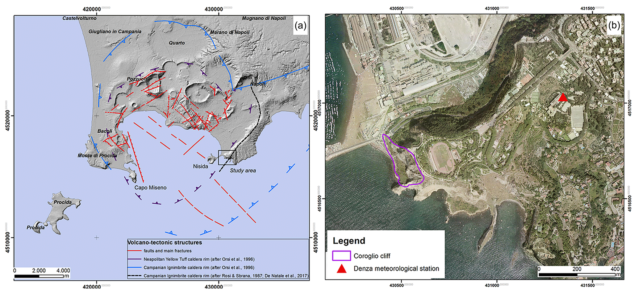
Figure 1 (a) Study area location and Phlegraean Fields area. (b) Detailed study area orthophoto (2004). The hillshade (a) and the orthophoto (b) in the background are from the year 2004 (courtesy of Regione Campania). Hillshade derives from a 5 m pixel DTM of the Carta Tecnica della Regione Campania (CTR) topographic map at 1:5000 scale, with 447 153 and 465 034 sheets (https://sit2.regione.campania.it/content/carta-tecnica-regionale-2004-2005; last access: 5 January 2020). The orthophoto is a mosaic of 447 153 and 465 034 orthophoto maps at the 1:5000 scale (https://sit2.regione.campania.it/content/ortofoto-campania-20042005; last access: 5 January 2020).

2 Site description

The analyzed sector of the Coroglio cliff (Figs. 1b and 2) is ∼140 m high and 250 m wide, with the aspect towards the SW. Different geological units and slope angles characterize the cliff (Fig. 3). The upper part displays slope angles varying from 35 to 45^∘ and is formed by stiff to loose Holocene pyroclastic deposits (LP unit) about 30 m in thickness, including a 2–3 m thick layer formed by very loose, reworked volcaniclastic deposits and soils at the top of the succession exposed on the cliff surface.

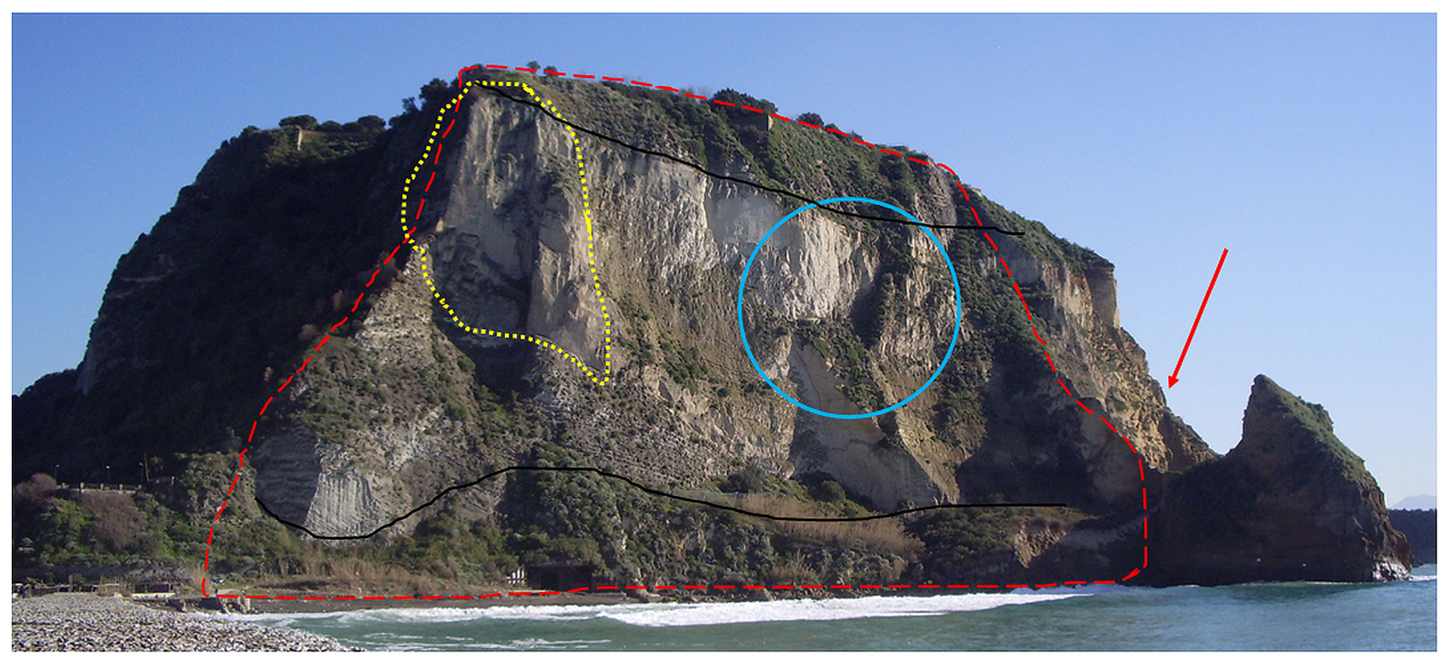
Figure 2 Coroglio cliff view from the WSW. The red dashed line shows the area mapped in Fig. 3, the yellow dotted line shows the area involved by reinforcement works, the light blue circle shows the area with unstable tuff blocks and the red arrow shows the detachment area of the failure that occurred around 1990, located outside the area mapped in Fig. 3. Black lines separate the upper, median and lower parts of the cliff.

The median part of the cliff is characterized by almost vertical slope and is formed by two tuffaceous units, separated by an angular unconformity. The Neapolitan Yellow Tuff (NYT) formation is a lithified ignimbrite deposit dated at ∼15 ka (Deino et al., 2004). The NYT represents the upper unit in the outcrop and is formed by alternating coarse-grained, matrix-supported breccia; thinly laminated lapilli beds; and massive ash layers. The NYT displays a relatively homogeneous texture with several sub-planar surfaces likely controlled by structural discontinuities and can be classified as weak to moderately weak rock (Froldi, 2000). The Trentaremi (TTR) formation forms an older tuff cone dated at ∼22.3 ka and represents the lower unit, consisting of slightly welded to welded, whitish to yellow, coarse-grained pumiceous fragments embedded in a sandy ash matrix and lapilli beds. Diffused decimeter-scale vesicles and vacuoles due to differential erosion, markedly controlled by the bedding of the pyroclastic deposits, characterize the TTR rock face. These forms are typically related to the weathering due to salty seawater and wind erosion (Ietto et al., 2015).

The tuff units cropping out at the Coroglio cliff are characterized by a complex system of mostly steep and planar structural discontinuities and fractures (Matano et al., 2016) showing highly variable spacing, well-developed NE–SW and NW–SE directions, and subordinate N–S and E–W trends. The base of the cliff is covered by slope talus breccia (dt), partly occurring directly along the shoreline. These deposits are produced by the frequent failures occurring along the cliff. The cliff instability is due to several causes, such as the complex volcano-tectonic evolution, the severe anthropic modifications (i.e., excavations, tunneling and so on) of the coastline since Roman times and weathering and erosion processes occurring at the boundary between coastal and marine environments. The last relevant tuff failures occurred around 1990 (Froldi, 2000) along the southern sector of the cliff (Fig. 2). Due to the severe instability conditions, the upper part of the northern sector of the tuff cliff was subject to reinforcement works (Fig. 2) at the beginning of the 2000s. These consisted in a wire mesh and steel cable network applied to the tuff wall steel reinforced with bars anchored and bolted to the rock.

During the first phase of the research, we have integrated the results of long-range terrestrial laser scanner (TLS) surveys with structural field mapping to obtain a detailed geostructural analysis and classification of the slope (Fig. 4) (Matano et al., 2016). Repeated TLS surveys have been used for obtaining a detailed multi-temporal digital terrain model (DTM) of the cliff (Caputo et al., 2018) that allowed mapping of the landslides that occurred during the period between 29 April 2013 and 4 March 2015 (Fig. 3). In detail, four types of landslides (rock fall, debris fall, earth flow and soil slip) have been recognized in the different sectors of the cliff (Fig. 3). These have caused a total eroded/fallen volume of about 3500 m³ of volcanic material (rock and soil), and the related short-term retreat rate of the entire cliff has been assessed at about 0.07 m yr⁻¹ during 2013–2015 (Caputo et al., 2018). Based on a geomorphological analysis, including cliff inspections carried out by climber geologists and interpretation of the multi-temporal DTMs, an area with several unstable tuff blocks (Fig. 2) has been recognized in the NYT unit sector of the cliff (Fig. 3). This area has been selected for implementing the monitoring system.

Figure 3 Geological vertical map of the Coroglio cliff (modified after Matano et al., 2016). Landslide types that occurred during the 2013–2015 interval (Caputo et al., 2018) are also shown. Geological units: LP, stiff to loose recent pyroclastic deposits and soils; LP-NYT, thin layer of LP deposits on NYT unit; NYT, Neapolitan Yellow Tuff; TTR, Trentaremi Tuff; dt, slope talus breccia and gravelly beach deposits.

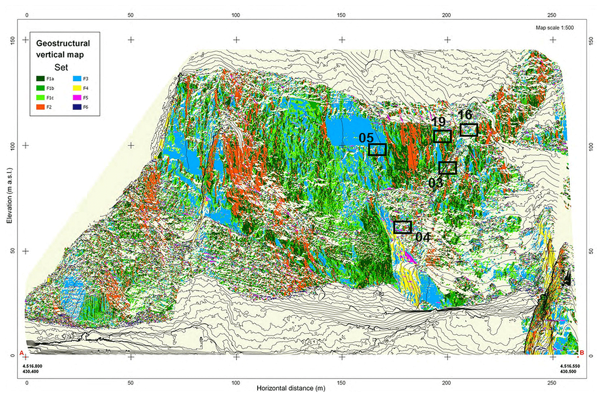
Figure 4 Geostructural vertical map (modified by Matano et al., 2016). Black boxes show location of the monitored unstable tuff blocks. Set legend (dip–dip direction): F1a (>65^∘/30–50^∘ and 220–235^∘), F1b (>65^∘/50–60^∘ and 235–245^∘), F1c (>65^∘/55–65^∘ and 245–255^∘), F2 (>65^∘/0–30^∘ and 180–220^∘), F3 (>70^∘/60–110^∘ and 255–280^∘), F4 (>70^∘/110–180^∘ and 300–355^∘), F5 (20–65^∘/50–195^∘) and F6 (<20^∘/0–360^∘).

3 Data and methods

3.1 The monitoring system

Based on the results of the geostructural and geomorphological surveys, a series of prismatic tuff blocks, bounded by open fractures, have been selected for the instrumental monitoring (Figs. 4 and 5). The accurate detection of structural discontinuities and morphometric parameters of the selected tuff blocks resulted in the understanding of the possible failure mechanism and their kinematic analysis. Volumes of the selected tuff blocks range between 4 and 15 m³, and the possible failure kinematics are toppling, planar and wedge sliding (Table 1).

Figure 5 Unstable tuff blocks of the NYT unit selected for monitoring activity (red lines).

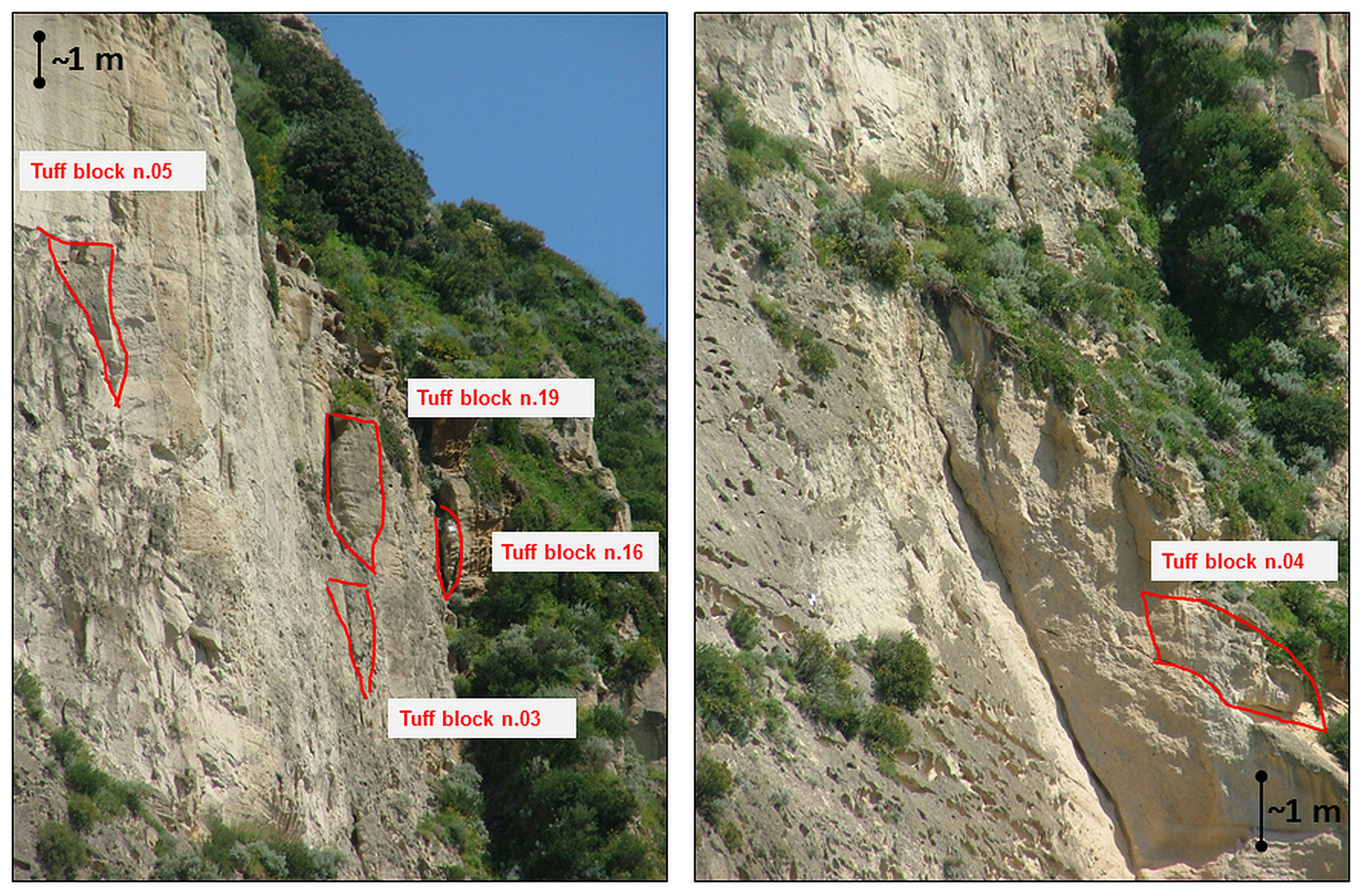
Figure 6 Data distribution of measurements of crackmeters (03F1, 04F1, 05F1, 05F2, 05F3, 16F1, 16F2, 19F1 and 19F2).

Table 1 Geostructural characteristics of the monitored tuff blocks.

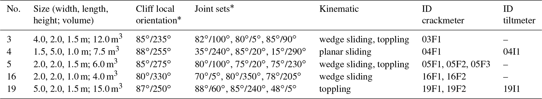
^∗ Orientation is expressed with dip and dip direction values in the format “dip/dip direction”.

The installed monitoring system consists of both standard geotechnical instruments, such as crackmeters and tiltmeters equipped with a near-rock-surface thermometer, installed in correspondence with the five selected unstable tuff blocks, and a weather station equipped with a thermometer, barometer, hygrometer, anemometer and rain gage sensors. The used instrumentation forms two separate linked sub-systems: the Coroglio cliff Monitoring System (CC-MoSys) and the Denza Meteorological Station (DeMS) (Fig. 1b).

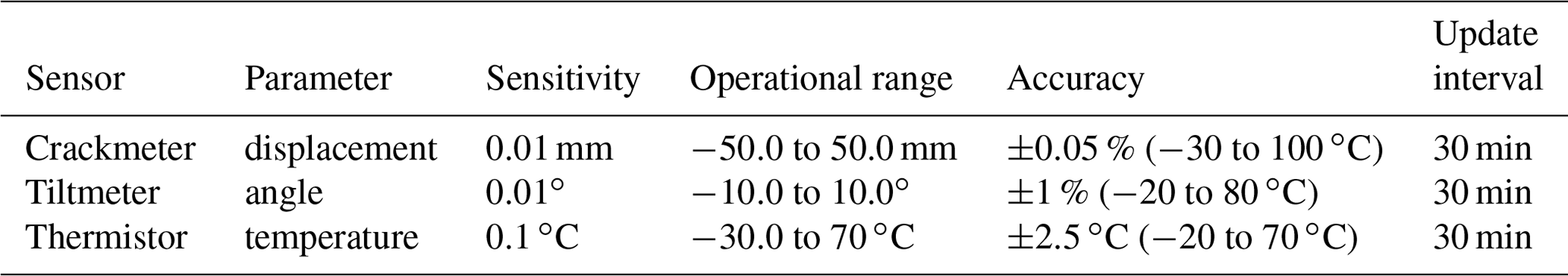
Specifically, the CC-MoSys is formed by nine monaxial electric crackmeters (model BOVIAR BTS LWG 100), one external thermistor (model BOVIAR NTC/A 10K) and two biaxial tiltmeters (model BOVIAR BIAX-B/T) equipped with internal thermistors (model BOVIAR NTC/A 10K) (Table 2). The geotechnical sensors have been installed across or on the face of the fractures bounding the five unstable tuff blocks in order to provide an accurate monitoring of displacements and rotations. Each sensor is individually cabled to the acquisition unit (model BOVIAR eDAS 16ch; see at: https://www.boviar.com/it/prodotti/centralina-di-acquisizione-dati-edas-2/, last access: 5 January 2020), located at the top of the cliff.

Table 2 Technical specifications of the sensors in CC-MoSys cabled with the acquisition unit – model eDAS 16ch.

The DeMSys is formed by a meteorological station (DAVIS, model Vantage Pro2 – wireless; see at: https://www.davisinstruments.com/support/vantage-pro2-wireless-stations/, last access: 5 January 2020), located less than 1 km away from the cliff (Fig. 1b), characterized by a wireless Integrated Sensor Suite (ISS) including barometer, hygrometer, pluviometer and thermometer integrated sensors and an anemometer (Table 3). The CC-MoSys tuff monitoring unit records 16 parameters (Table 4) with a frequency set to 30 min for 48 daily measures. The weather station unit records nine parameters (Table 5) with a frequency of measurements set up 10 min for 144 daily measures. Continuous data recording of geotechnical sensors was active from December 2014 to October 2018, whereas the weather station has been active since January 2014. The meteorological time series analyzed in this work are updated to December 2018. The monitoring system has been regularly controlled and maintained so as to ensure full accuracy in measures, even if some missing data intervals are present due to the occurrence of some functional interruptions of the acquisition units.

Table 3 Technical specifications of the sensors of the used meteorological station – model DAVIS Vantage Pro2 wireless in DeMS.

Overall, the monitored parameters include both deformation and meteorological ones:

• variation in the cracks' opening and displacement (sliding) along tuff cracks,

• slope angle variations (rotation) in tuff block surfaces,

• air temperature and near-rock-surface air temperature,

• humidity,

• wind (velocity and direction),

• barometric pressure,

• rainfall (rain quantity and rate).

The data acquisition and broadcasting system is fully remotely controlled. Rechargeable batteries and a solar panel provide the power supply for the monitoring system. Twice a day, the measured data are transferred via a GSM (Global System for Mobile Communications) network to a master station located in the ISMAR (Istituto di Scienze Marine) research institute, where data are directly stored in a dedicated NAS (network-attached storage) system and converted to open-access files for our data repository.

3.2 Tuff deformation data

The deformation data consist of measurements of displacement across the fractures bounding tuff blocks along the direction of the crackmeters' axis and of both horizontal and vertical angles associated with rotation of the rock blocks (Table 2). The instruments have collected measurements every 30 min for a period of about 4 years. These measurements are expressed for each sensor as relative measurements with respect to the initial measurement, considered to be a reference zero value. We also measured near-rock-surface air temperature (as a proxy for surface rock temperature) using some thermistors installed at three locations on the cliff (i.e., near the acquisition unit and near the tiltmeter boxes). In this way, the CC-MoSys database encompasses 67 355 measurements acquired for 1404 d (from 3 December 2014 to 6 October 2018). Some missing data intervals are present due to the occurrence of some functional interruptions of the eDAS acquisition unit; for two sensors (F04F1 and F16F2), missing data intervals are larger (Table 6) due to the occurrence of mass movements on the cliff that damaged the two sensors.

We compute some descriptive statistics for summarizing the different features of the deformation measurement dataset (Table 6). These statistics are the results of a univariate analysis, describing the distribution of each single variable, including its central tendency (mean and median) and data dispersion (including minimum and maximum values, quartiles, and standard deviation).

Table 4 List of measured tuff deformation parameters in CC-MoSys.

Table 5 List of measured meteorological parameters in DeMSys.

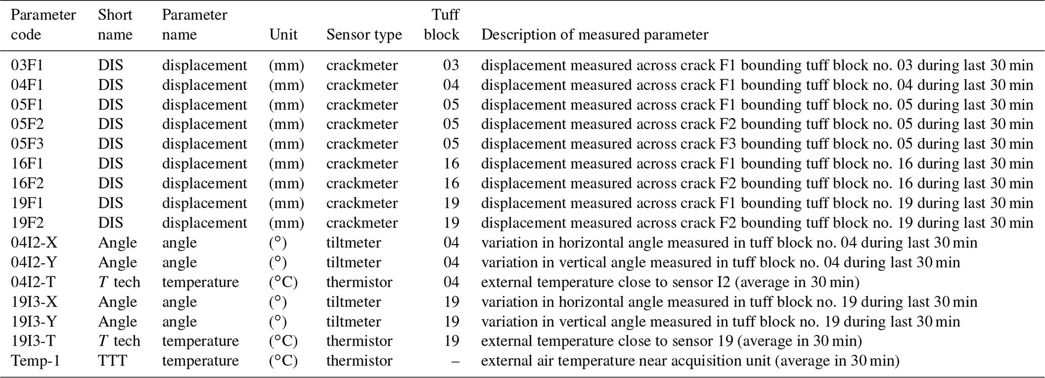
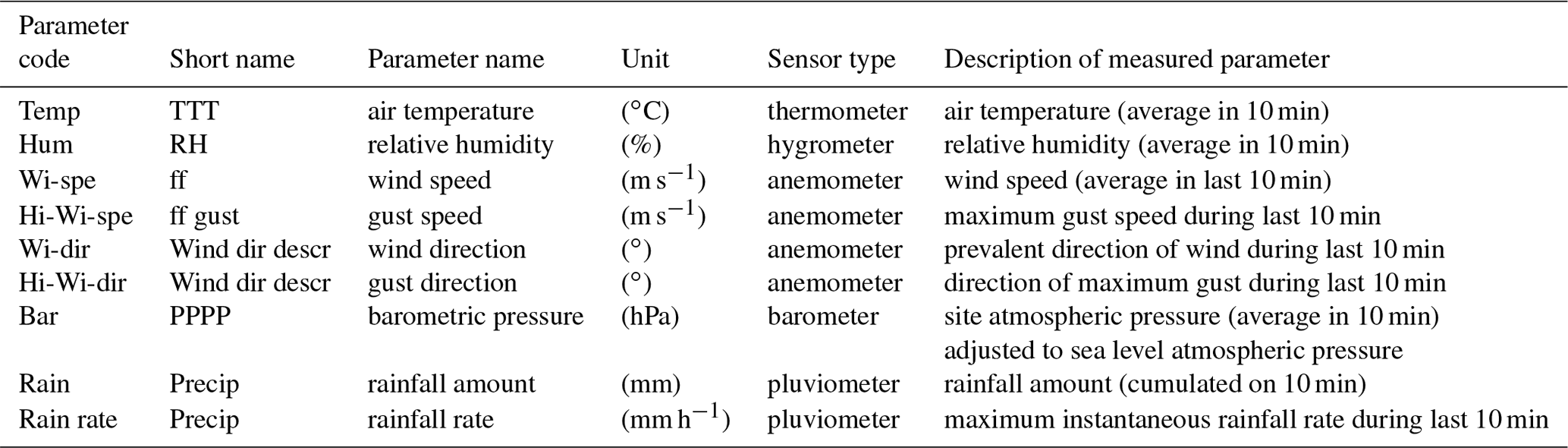
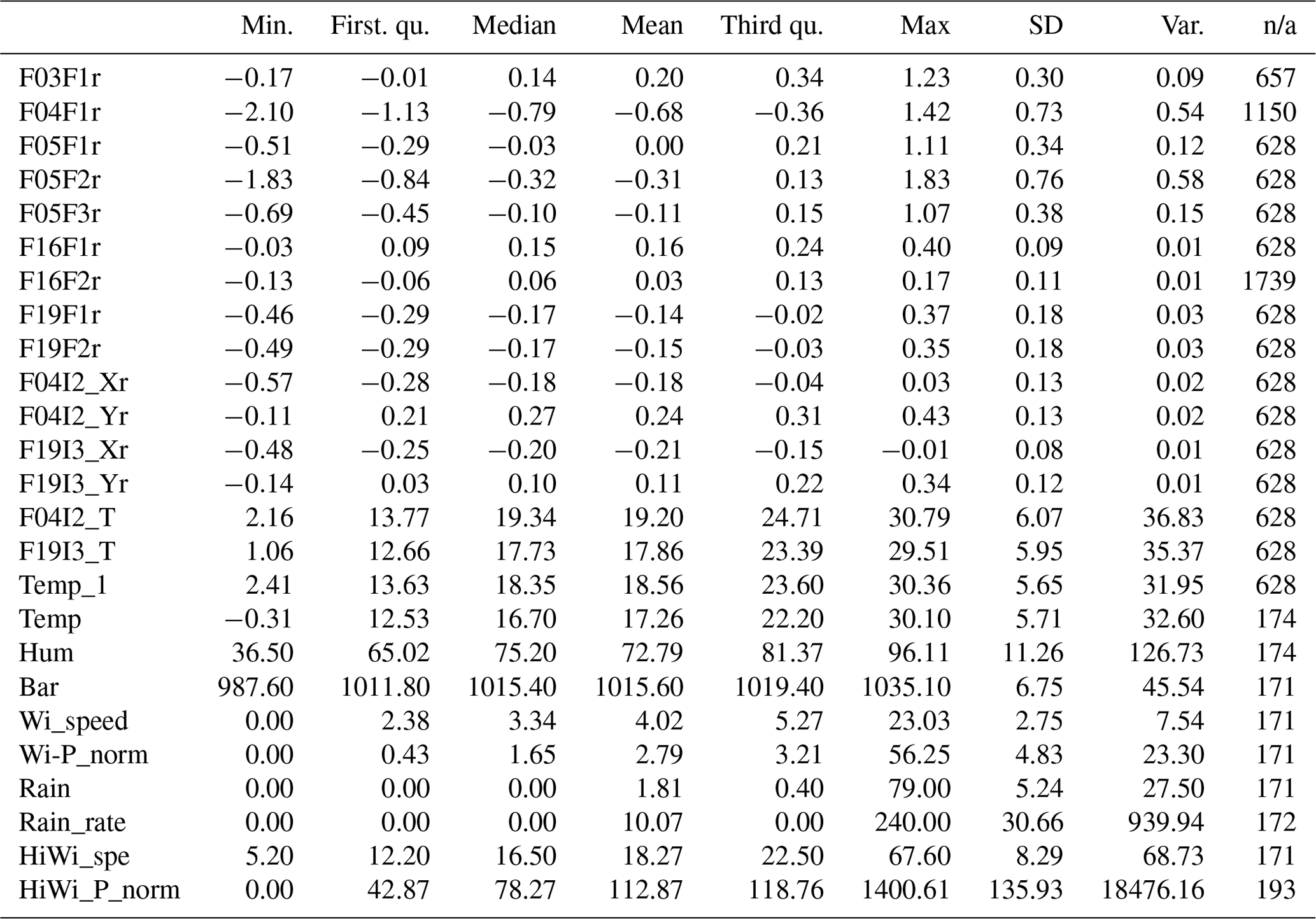
Table 6 Descriptive statistics of tuff deformation data and temperatures measured by CC-MoSys.

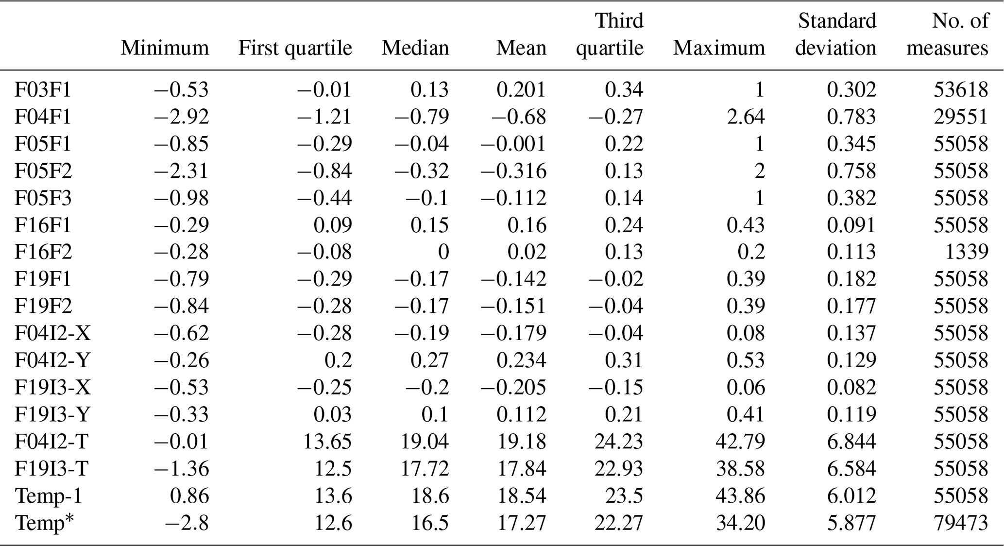
^∗ Temp data, measured by DeMSys from 1 January 2013 to 31 December 2018, have been aggregated to 30 min for comparison with CC-MoSys temperature data.

3.3 Meteorological data

The database of DeMS measurements (Fortelli et al., 2019) encompasses 262 944 measurements acquired with a 10 min interval for 1826 d spanning from January 2014 to December 2018.

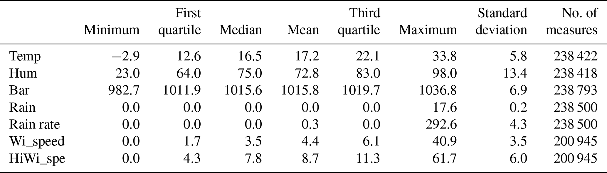
Some missing data intervals are present due to the occurrence of some functional interruptions of the DAVIS acquisition unit; the missing data intervals are larger only for the anemometric sensor data (i.e., Wi_speed and HiWi_spe) due to a technical issue of the sensor during 2018. The descriptive statistics resulting from a univariate analysis of the acquired dataset, with the exception of wind and gust direction, are shown in Table 7.

Table 7 Descriptive statistics of temperature and meteorological data measures by DeMS.

We added to the database two numeric parameters that take into account the direction of wind and gust, i.e., wind pressure (Wi-P_norm) and gust pressure (HiWi-P_norm), expressed in newtons per square meter. They are for the normal component of the pressure exerted by the wind/gust on the rock face on the cliff. We calculated the normal component of the wind velocity by considering the angle between cliff average aspect orientation, that is towards the WSW (i.e., 247.5^∘), and the wind/gust direction. Winds blowing from the direction of 337.5 to 360^∘ and from 0 to 157.5^∘ do not produce pressure on the rock surface, as they are sheltered from the cliff itself. Winds blowing from directions between 157.5 and 337.5^∘ produce a normal component of pressure that varies under the cosine of the incidence angle with the cliff (ranging from 0 to 90^∘). Once we have calculated the vertical component of the wind/gust, we may calculate the wind/gust pressure normal to the cliff with the simplified formula (ASCE, 2013)

$$\begin{array}{}\text{(1)}& P_{\text{n}}=\mathrm{0.613}{\mathrm{veln}}^{\mathrm{2}},\end{array}$$

where P_n is wind/gust pressure normal to the cliff expressed in newtons per square meter, veln is wind velocity normal to the cliff expressed in meters per second, and 0.613 is the coefficient based on average values of air density and gravitational acceleration expressed in reciprocal kilograms per meter.

4 Results

4.1 Deformation trends

Crackmeter data usually show value ranges between 0.48 and 1.98 mm, with the two relevant exceptions of 04F1 and 05F2 with ranges of 5.56 and 4.31 mm, respectively. Tiltmeter data show a lower variability as value intervals range between 0.38 and 0.78^∘ (Table 6). In more detail, the data distribution analysis shows some different trends for the data of the different sensors (Fig. 6). Data of the 03F1 sensor show an asymmetric distribution with a modal value around −1 mm and higher coda values up to 3 mm. The 04F1 data show a uniform distribution between −0.1 and 3 mm. Parameters of block 05 have a very large range of variability, with a well-defined main value only for F2 sensor. F1 and F3 sensors show a very high correlation (Fig. 7), suggesting a uniform behavior of the crack in the section covered by them. All three sensors recorded large distribution of both positive and negative values, indicating a strong dynamic behavior. On the other hand, the 16F1 sensor (Fig. 6) shows a mono-modal distribution well centered around 0.2 mm (with an oscillation of ±0.1 mm). The stability of the values across time could highlight a stable dynamic position reached from the block. The 16F2 sensor worked for a very short time compared with the others. However, the data distribution shows two main values of 0.0 and 0.2 mm. The F1 and F2 sensors, located on tuff block 19, show a quite identical behavior (Fig. 6). The similarity in recorded values suggests a uniform behavior of the lateral crack.

Figure 7 Correlation plot between 05F1 and 05F3 data.

The tiltmeter data have been reported in Fig. 8 for 04I2 and 19I3 sensors. The X (horizontal) components recorded prevalently negative variation, while the Y (vertical) components were positive over the entire time interval of the datasets. This evidence shows how the rock block moves and turns during the time to some preferred position (the higher histogram bar). For the 19I3 sensor, a small range of variability has been observed, about 0.4^∘, and a tiny distribution around 0.3–0.4^∘ for the Y component. A similar behavior is shown by component X where the equilibrium position is characterized by angle values between −0.2 and −0.3^∘.

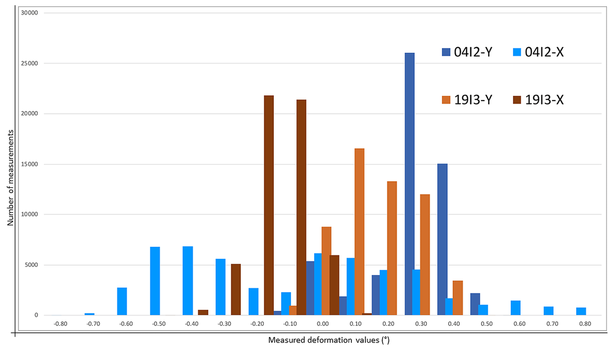
Figure 8 Data distribution of measurements of tiltmeters (04I2-X, 04I2-Y, 19I3-X and 19I3-Y).

The temperature value distribution of the three thermistors appears coherent and well centered in a range between +13 and +25 ^∘C (Fig. 9). If we compared those temperature data with air temperature measurements provided by the weather station installed in the vicinity (Fig. 10), time series show, as usual for this climatic region, clear seasonal variation patterns and annual cyclicity with some small differences. In detail, near-rock-surface air temperatures show minimum values from 2.8 to 3.7 ^∘C higher and maximum values from 4.4 to 9.7 ^∘C higher than air temperatures (Table 6). Amplified near-rock-surface air temperatures could result in consequent increases in crack deformation forces.

Figure 9 Data distribution of measurements of thermistors (19I3-T, 04I2-T and Temp-1).

If we consider the time distribution of measured data, both crackmeters and tiltmeters show several evidence of tuff deformation through time. The time series of the measured crack aperture and plane rotation data reveal a deformation pattern characterized by both diurnal and seasonal cyclical deformation (Figs. 11 and 12). The data plots for a single year of measurements show a similar repetitive pattern with lower values in late winter and higher values in late summer (Fig. 13), showing significant correlation with seasonal temperature trends. Some trends of cumulative multi-annual changes, based on about 4 consecutive years of data (December 2014 to October 2018), can also be recognized. Crackmeters show from +0.1 to +1.2 mm cumulative deformation (Fig. 11), while tiltmeters show from 0.1 to 0.4^∘ cumulative angle variation (Fig. 12).

Figure 10 Temperature time series showing daily, seasonal and annual variation patterns. Long-term trends, based on about 5 consecutive years of data, show annual cyclicity. Air temperature and near-rock-surface air temperature are fully synchronous; peaks in near-rock-surface air temperatures (19I3-T, 04I2-T and Temp-1) are sometimes higher than those of air temperature (Temp). Data are incomplete in some months.

Figure 11 Crack aperture variation time series showing daily, seasonal and annual deformation patterns. Long-term trends, based on about 4 consecutive years of data (December 2014 to October 2018), show from +0.1 to +1.2 mm of cumulative deformation. Data are incomplete in some months.

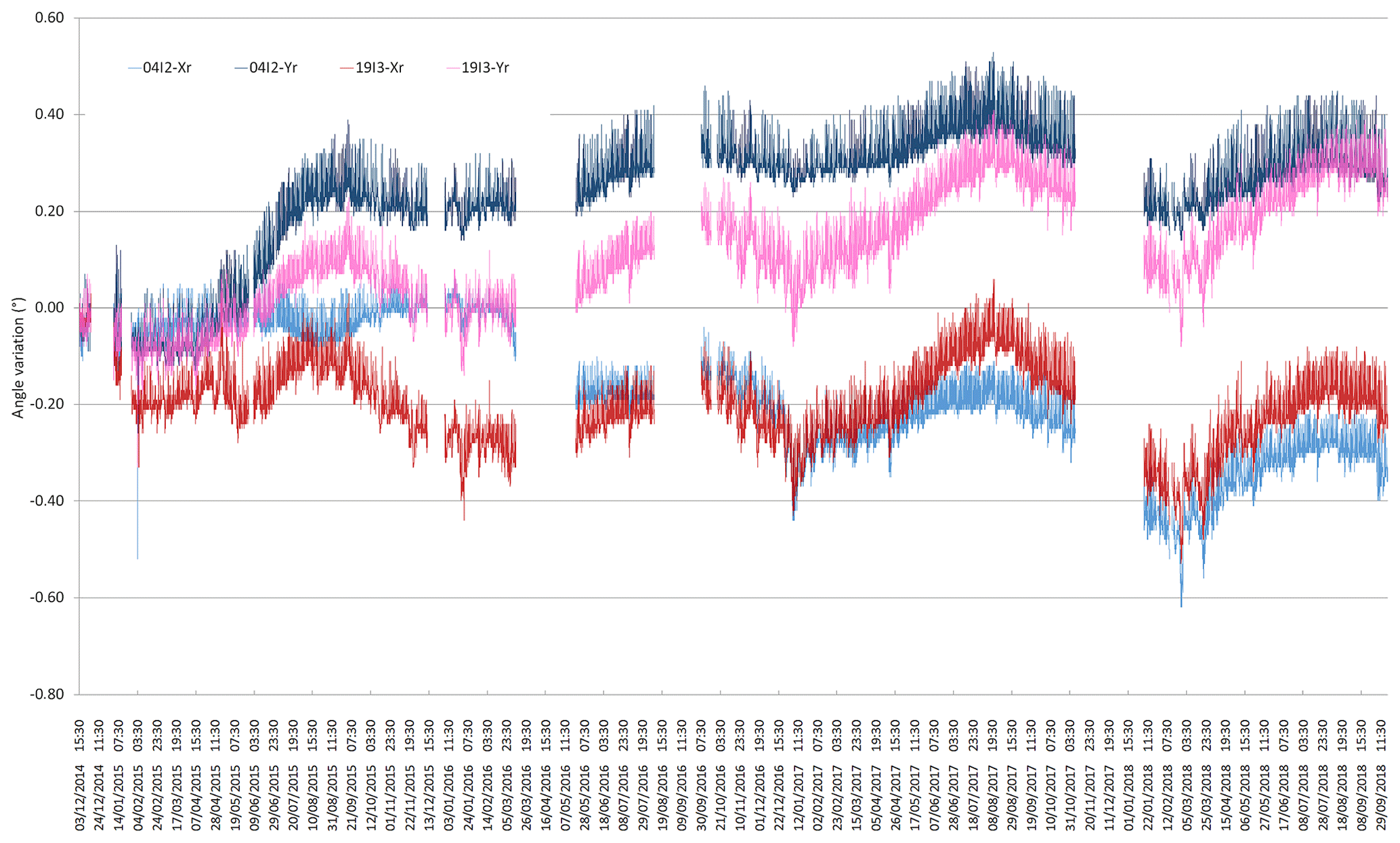
Figure 12 Angle variation time series data showing daily, seasonal and annual deformation patterns. Long-term trends, based on about 4 consecutive years of data (December 2014 to October 2018), show from 0.1 to 0.4^∘ of cumulative angle variation. Horizontal and vertical angle variation shows opposite evidence for each block. Data are incomplete in some months.

4.2 Thermal trends

Temperature time series data (Fig. 10) show a clear seasonal cyclicity and inter-annual variation patterns. Air temperature values range between −2.9 and 33.8 ^∘C throughout the 5 years of measurements.

Average temperature values of the 5-year period have been plotted for the average daily value analysis, daily minimum temperature (T_min) and daily maximum temperature (T_max) in order to observe the annual trends and detect the most significant surplus or deficit thermal phases (Fig. 14). Diagrams also report interpolation curves relative to minimum and maximum daily values (fourth-grade polynomial equation); we also computed the difference between the minimum and maximum temperatures (ΔT).

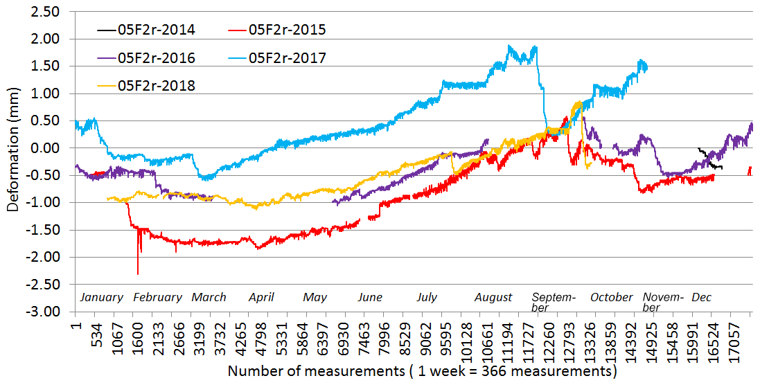
Figure 13 Annual time series plots of the 05F2 crackmeter showing partly repetitive seasonal deformation patterns.

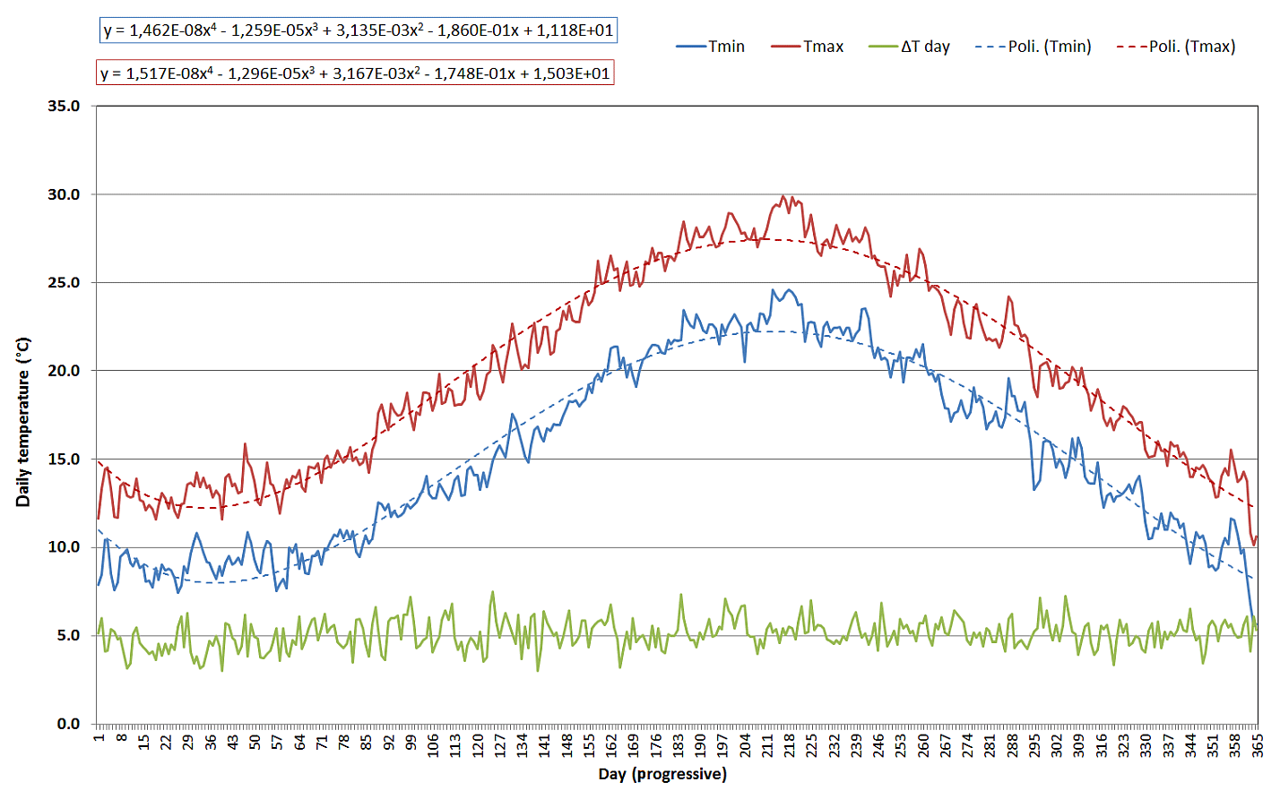
Figure 14 Average daily thermal trend, for 2014–2018, recorded by Denza weather station with fourth-grade polynomial equations. Maximum temperature values are indicated with a red line, minimum values with a blue line and daily temperature range with a green line.

In detail, we have evaluated the thermal increase between the late winter minimum and summer maximum and the autumn thermal decrease between the summer maximum and late December minimum. From the analysis of fourth-grade polynomial equations of annual thermal trend, relative to daily T_min and T_max, the following values have been derived:

•  

  T_min(1) (min) = 8.0 ^∘C (05/02)
  T_max(1) (min) = 12.3 ^∘C (04/02)

•  

  T_min (max) = 21.9 ^∘C (30/07)
  T_max (max) = 27.5 ^∘C   (02/08)

•  

  T_min(2) (min) = 7.9 ^∘C (31/12)
  T_max(2) (min) = 12.2^∘ C  (31/12).

Thermal yearly excursions are therefore equal as follows.

•  

  Spring thermal increase is
  ΔT+ (min) = T_min (max) – T_min(1) (min) = 13.9 ^∘C,

  ΔT+ (max) = T_max (max) – T_max(1) (min) = 15.2 ^∘C.

•  

  Autumn thermal decrease is
  ΔT− (min) = T_min (max) – T_min(2) (min) = 14.0 ^∘C,

  ΔT− (max) = T_max (max) – T_max(2) (min) = 15.3 ^∘C.

The main features highlighted by the analysis are the following:

• an annual trend showing a wave characterized by a weak thermal excursion, for both minimum and maximum daily values, probably associated with the proximity to the sea;

• a summer season with only a few days with daily maximum temperature above the threshold value of 30 ^∘C;

• an extremely mild winter season, with only a few days with minimum temperatures below 5 ^∘C;

• a weak daily thermal excursion, with values of generally ∼5 ^∘C and only a few days with a daily thermal excursion >10 ^∘C.

In detail, the annual thermal trend in the analyzed period is characterized by 3 years (2016–2018) with values close to the average values of the investigated period and 2 years with significant differences during the summer season. In detail, summer 2014 had values significantly lower than the average values, and summer 2015 had values characterized by a clear thermal surplus during the months of July and August, when the threshold value of 30 ^∘C was exceeded on 22 d. During winter there were not any long periods characterized by significantly low temperatures, with the two exceptions of the period between 5 and 15 January 2017 (with values close to zero and a minimum of −1.6 ^∘C) that also caused weak snowfalls, and a very cold and snowy phase at the end of February 2018.

4.3 Rainfall trends

Rain and rain rate data time series are plotted in Fig. 15. Rainfall is characterized by a considerable irregularity, with sometimes extremely high accumulation values and rates (October 2015, September 2017) usually associated with late summer storms, alternating with periods of modest rainfall even in seasonal phases in which rainfall is generally abundant (December 2015 and 2016). Rainfall (measured at intervals of 10 min) reached a maximum value of 17.6 mm on 12 September 2014, corresponding to a rain rate of 105.6 mm h⁻¹. The maximum rain rate of 292.6 mm h⁻¹ was recorded on 19 September 2016.

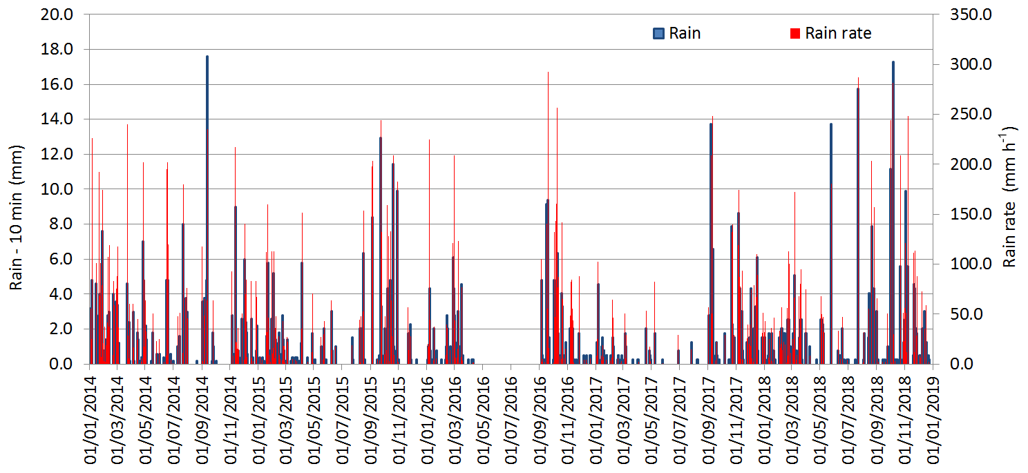
Figure 15 Rain amount (10 min) and rain rate time series data showing daily, seasonal and annual variation patterns in the Denza station during 2014–2018.

We plotted the average values for the whole 5-year period of the monthly total rainfall amounts (Fig. 16). In order to evaluate the occurrence of rainfall surplus or deficit periods, these values are compared with the monthly average values of rainfall, for the 1872–2005 time period, measured at the Meteorological Observatory (MOUF) of the University of Napoli “Federico II” (Mazzarella, 2006). It is worth noting that the monthly precipitation average values over the analyzed 5-year period (2014–2018) tend to converge towards those values of climatological relevance recorded in Naples at MOUF (Mazzarella, 2006), thus reflecting the strong pluviometric characterization of the site. Data analysis highlights some peculiarities in the rainfall conditions that affect the area. The average annual rainfall amount of 759.6 mm is below the amount of the climatological reference of 866.0 mm. In detail, the summer rainfall amount is almost equal to the MOUF climatologic reference (69.0 mm vs. 75,7 mm), while spring (149.3 mm vs. 181.4 mm), autumn (281.9 mm vs. 317.6 mm) and winter (259.4 mm vs. 290.9 mm) rainfall amounts are slightly below the MOUF climatologic reference. The winter precipitation deficit is due to a strong negative rain anomaly observed at Denza during December 2015 (0.3 mm) and 2016 (9.5 mm). During 2015, a rainfall regime with a large prevalence of dry months was compensated for by 3 very rainy months, January, February and October, the last one characterized by a rainfall amount of 195.5 mm. The year 2017 has been characterized by a severe rainfall deficit with a total annual precipitation amount of 536.8 mm; in particular, summer 2017 rainfall was only 4.1 mm, suggesting extremely dry conditions for this season. Instead, the year 2018 has been characterized by a total annual rainfall amount of 902.1 mm, slightly above MOUF climatologic values.

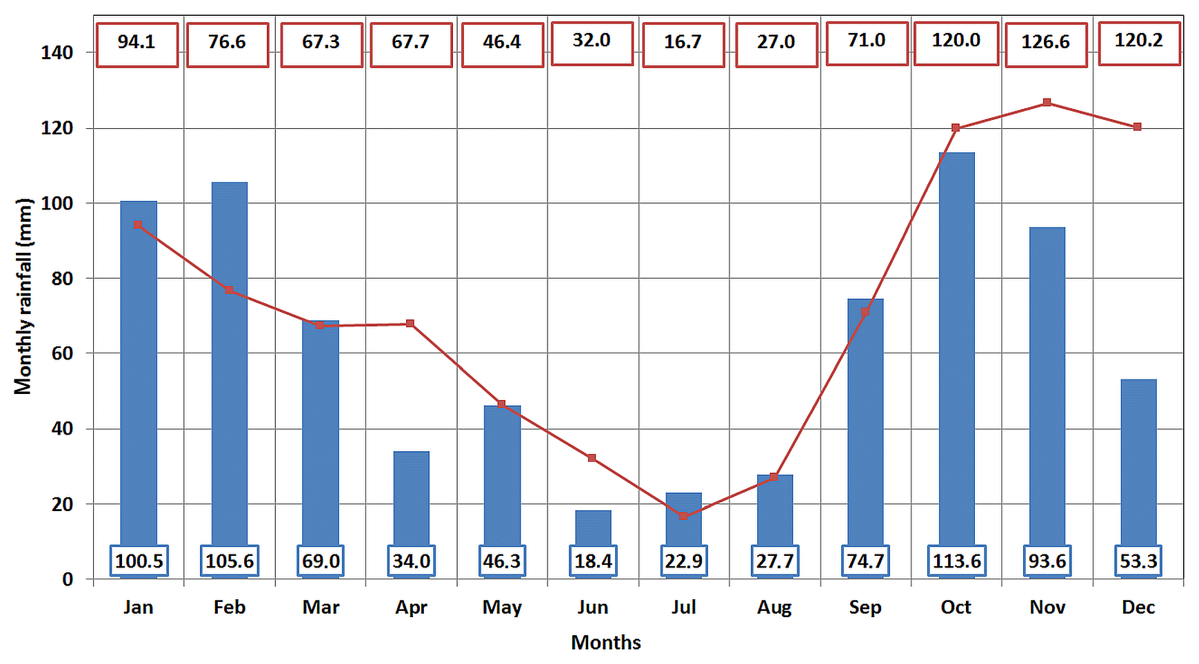
Figure 16 Average cumulative monthly rainfall data histogram for 2014–2018. Diagram also reports average monthly values of rainfall, measured at the Meteorological Observatory of University of Naples “Federico II” since 1872 (Mazzarella, 2006). Rainfall values are reported in blue square cells and red square cells.

4.4 Wind trends

Wind and gust speed data time series are plotted in Fig. 17. Wind velocity and gust velocity (both measured at 10 min intervals) reached the maximum values of 40.9 kn (11.8 m s⁻¹) and 61.7 kn (31.7 m s⁻¹), respectively (Table 7).

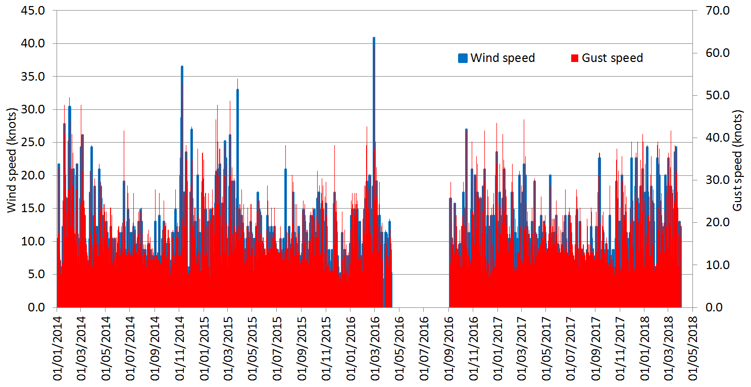
Figure 17 Wind and gust speed time series data showing daily, seasonal and annual variation patterns at the Denza station during 2014–2018.

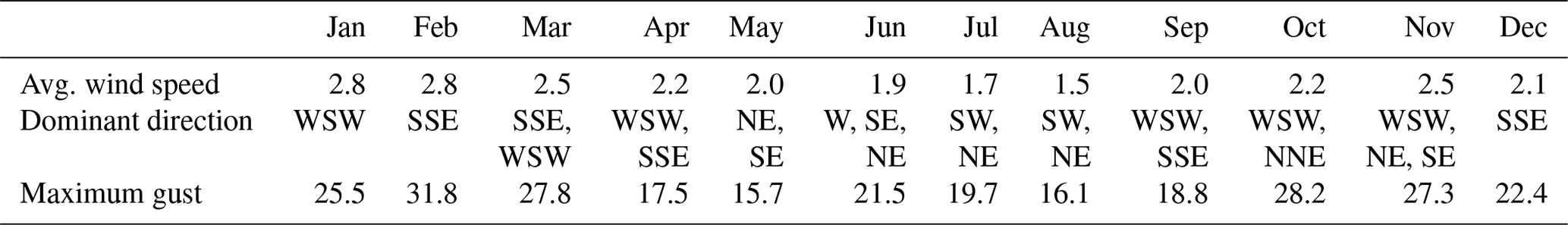
The wind regime indicates considerable consistency, both in terms of anemoscopic regime (wind provenance direction) and in terms of average intensity. The seasonal regimes are characterized by the repetition of the anemometric patterns, highlighting the occurrence of local structural factors that, even if in interaction with the meteorological conditions on a synoptic (cyclonic) scale, are able to control the wind regime in the considered coastal sector. Tables 8 and 9 summarize the annual and monthly average values of average wind speed (m s⁻¹), dominant direction of the wind (sector of 22.5^∘) and maximum wind gust (m s⁻¹). Wind average speed can usually be categorized as level 2 on the Beaufort scale, while gust maximum speeds can be categorized as levels from 9 to 11 on the Beaufort scale.

Table 8 Annual average values of wind measures during 2014–2018.

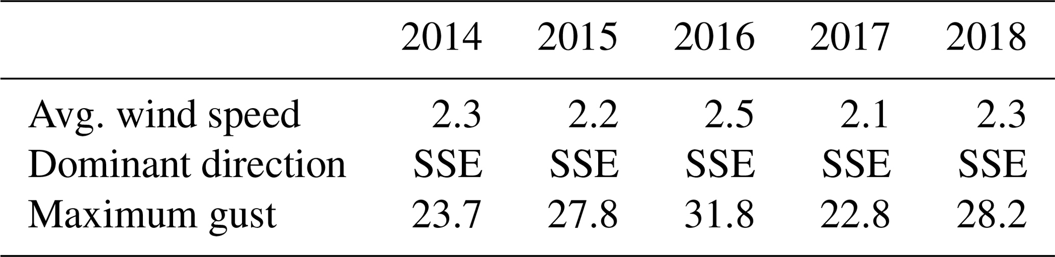
Table 9 Monthly average values of wind measures during 2014–2018.

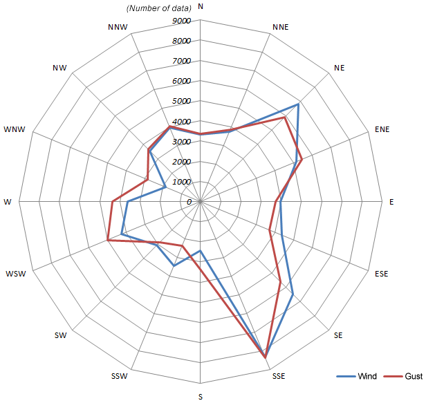
The wind rose diagram of Fig. 18 shows the frequency distribution of wind and gust directions, which are mainly from the SSE, NE and WSW. During spring, the synoptic winds blow with greater frequency from the second and fourth quadrants of the rose diagram, with the SE direction reaching the maximum percentage weight. The direction associated with the maximum average wind speed values is the SE–SSE directions. Therefore, we may infer that the spring season is characterized by the alternation of south-eastern and north-western winds, which are also associated with the greatest average intensities. The polar diagram shows that summer winds blow with a prevalence from the third and fourth quadrants, with the WSW direction reaching the maximum percentage weight. The directions associated with the maximum average wind speeds are the westerly ones. It is therefore possible to state that the summer season is dominated by breeze regime winds, typical of the coastal Mediterranean areas. However, it is worth underlining that the occurrence of SSE relatively high average intensities is not infrequent. In the autumn season winds blow in a well-distributed pattern in all sectors, with the SE–SSE direction reaching the maximum percentage weight; also, the directions associated with the maximum average wind speeds are the SE and SSE. It is therefore possible to state that the autumn season is normally dominated by Scirocco-like anemometric events, with associated very rough sea. During the winter season, the polar diagram highlights an anemoscopic regime very similar to the autumn one. In fact, it may be observed that the synoptic winds blow in a well-distributed way involving quadrants one, two and four, with the SE and NE directions reaching the maximum percentage weight. The provenance directions associated with the maximum average wind speeds are namely SE and SSE.

Figure 18 Frequency distribution of wind and gust directions measured during 2014–2018.

By considering the angle between wind/gust direction and Coroglio cliff aspect, we have calculated the values of the normal component of the wind/gust pressure with respect to the rock face exposed on the cliff, i.e., wind normal pressure (Wi-P_norm) and gust normal pressure (HiWi-P_norm) (Fig. 19). Wind and gust normal pressure reached the maximum values of 185.6 and 1400.6 N m⁻², respectively.

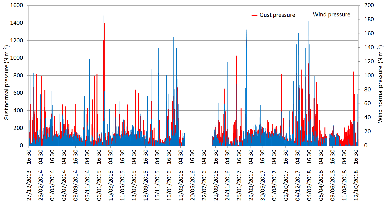
Figure 19 Wind and gust normal pressure time series data showing daily, seasonal and annual variation patterns at the Denza station during 2014–2018.

4.5 Humidity and barometric pressure trends

Humidity and barometric pressure data time series are plotted in Fig. 20. Relative humidity values range between 24.7 % and 98.0 % with mean values around 72.8 % (Table 7). The monthly, seasonal and annual trends are characterized by similar, repetitive patterns with usually high values between 70 % and 80 %. This is a direct consequence of the closeness to the sea surface and of forced lifting of air masses due to the orographic factor, leading to a cooling with an associated increase in relative humidity. The barometric pressure values range between 983.2 and 1036.7 mm with mean values around 1015.6 mm (Table 7). The seasonal and annual trends are characterized by similar, repetitive patterns, showing a high variability of values during the 6-month cold period and a lower one during the warm period; this is due to the synoptic-scale meteorological perturbations frequently affecting the area.

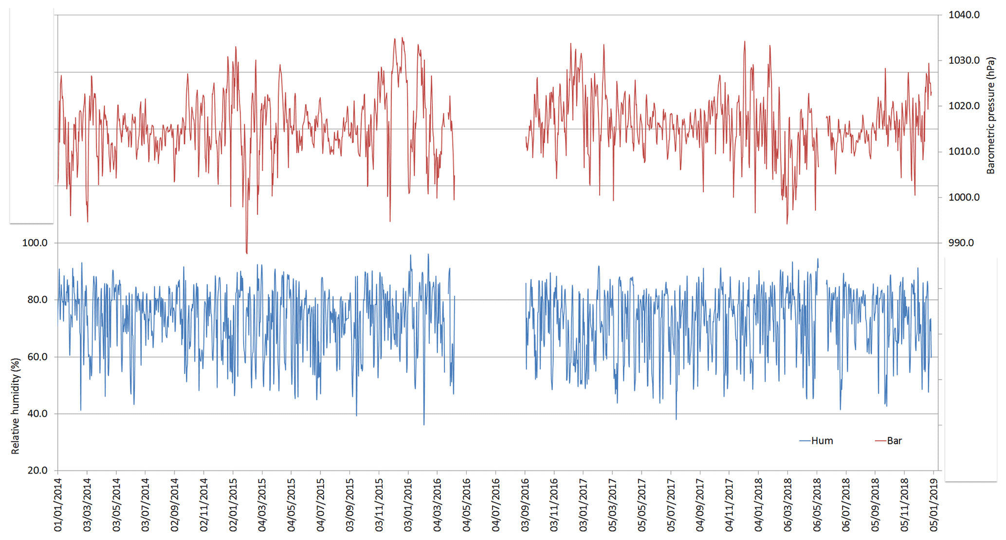
Figure 20 Barometric pressure and humidity time series data showing seasonal and annual variation patterns at the Denza station during 2014–2018.

5 Correlation and regression analysis of data

Tuff deformation measurements have been collected at 30 min intervals whereas the meteorological data have been recorded at 10 min intervals. Successively, we have analyzed the correlations among the time series of the different parameters. Therefore, we have aggregated the data into 1826 daily records (from 1 January 2014 to 31 December 2018). We have calculated the daily average values for all deformation data and partly for meteorological data; in detail, we have calculated the highest daily value for the “Rain_rate”, “HiWi_spe” and “HiWi_P_norm” variables; the cumulative daily value for the “Rain” variable; and the daily average values for the others. The daily descriptive statistics are shown in Table 10.

Table 10 Descriptive statistics of daily tuff deformation and meteorological data.

In a multivariate perspective, we have examined the correlation among tuff deformation parameters and meteorological variables in order to detect possible relationships between the two datasets. We have computed the correlation matrix, where the Pearson correlation coefficient is the generic element. This coefficient varies between −1 (maximum negative correlation) and +1 (maximum positive correlation). In particular, correlations greater than $\left|\mathrm{0.5}\right|$ are regarded as highly significant, whereas a coefficient between $\left|\mathrm{0.33}\right|$ and $\left|\mathrm{0.5}\right|$ is considered slightly significant.

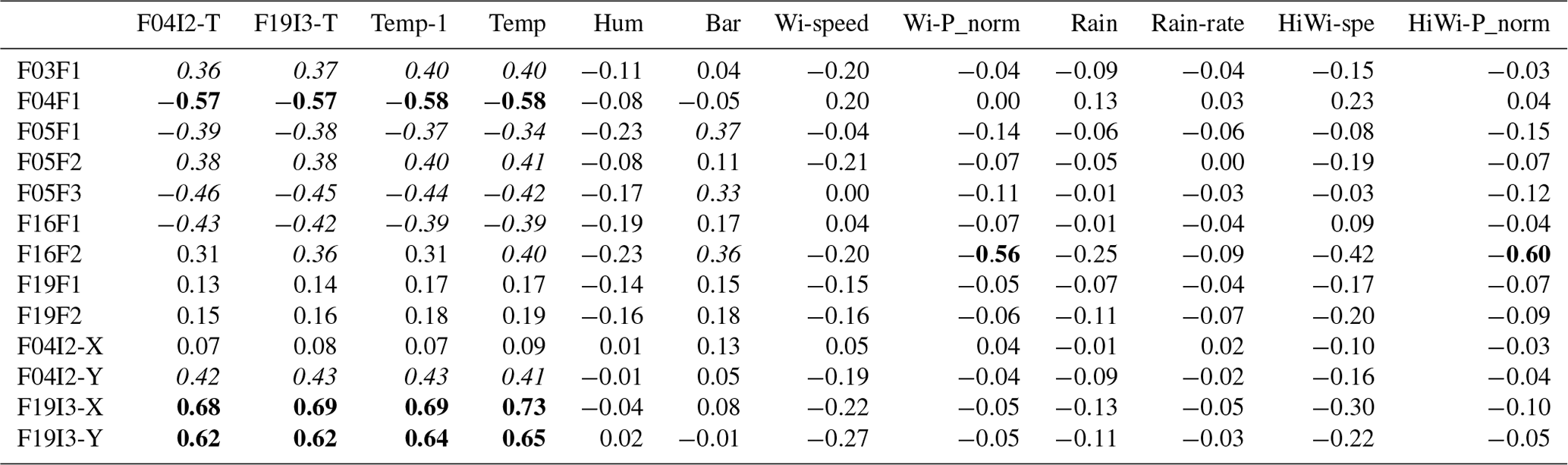
Table 11 shows a part of this matrix related to the correlations. We have observed that the highest positive correlations are between F04F1 and Temp (0.73), and all the correlations between F19I3-X and the temperature variables are very high. Other deformation variables (F04F1, F19I3-Y) are very positively correlated with all the temperature variables. On the other hand, the variable F16F2 shows a high negative correlation with two meteorological variables related to the measure of wind Wi-P_norm (−0.56) and HiWi_P_norm (−0.60). Moreover it can be observed that most of the other variables associated with the deformation of the tuffaceous rocks show a correlation (even if lower) with the temperature variables, while the other meteorological variables display no correlation at all with the tuff deformation parameters (with the exception of a slight correlation with barometric pressure).

Table 11 Correlation matrix of tuff deformation and meteorological data; the correlations greater than $\left|\mathrm{0.5}\right|$ or $\left|\mathrm{0.33}\right|$ are in bold or italics, respectively.

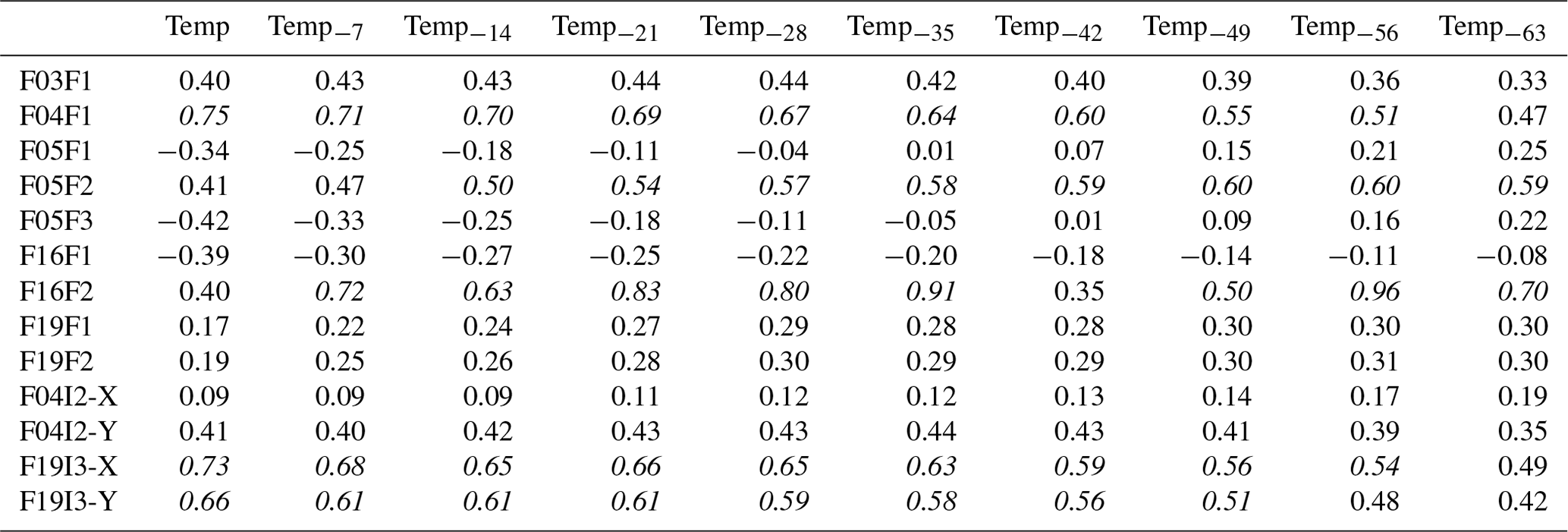
We have further investigated the relationship between the deformation and the temperature variables. Therefore, we have computed the correlation at different lags in order to evaluate the effect of the temperature over time. In particular, we have shown, in Table 12, the correlation among all the deformation variables and the air temperatures Temp at different lags (from 7 to 63 d, i.e., 1 to 9 weeks of delay), where the lag is expressed in number of days prior to the measurement of the deformation. It can be noted that the variables F04F1, F19I3-X and F19I3-Y show a positive correlation with the air temperature at almost all different lags. Therefore, we have suggested that there is a long-delayed time effect among them. Moreover, when we observe the different lags, a correlation between the F05F2 and F16F2 variables and the air temperature becomes evident. Overall, the correlation results increased within lags of 14–35 d.

Table 12 Correlation matrix between tuff deformation data and air temperature for different time lags (expressed in number of days). The correlations greater than 0.5 are in italics.

Based on the observation of the daily sample, we have decided to test the dependency of the deformation on the two meteorological factors: temperature and wind pressure. The correlations between the variables measuring temperature and the variables measuring the wind pressure show negative and very low values (e.g., −0.54 between Temp and Wi-P_norm and −0.08 between Temp and HiWi-P_norm). Obviously, all variables measuring both temperature and the wind effects are internally consistent and highly self-correlated. Therefore, we can perform a regression model where the dependent variable is the deformation measured by the variable F04F1, and the explicative variables are Temp and Wi-P_norm.

The model shows (Table 13) an adjusted R square of 0.63, so the linear model displays a high goodness of fit. Furthermore, the model is statistically significant (as p values show). In Table 14 we have reported the estimates of model coefficients. Both the coefficients are significant as shown by the p values. We have also observed a positive effect of both variables on the deformation at a daily level. Therefore, we have inferred that the deformation increases if temperature and wind effect increase and the variation is defined by the values of the two regression coefficients.

Table 13 Analysis of variance (ANOVA).

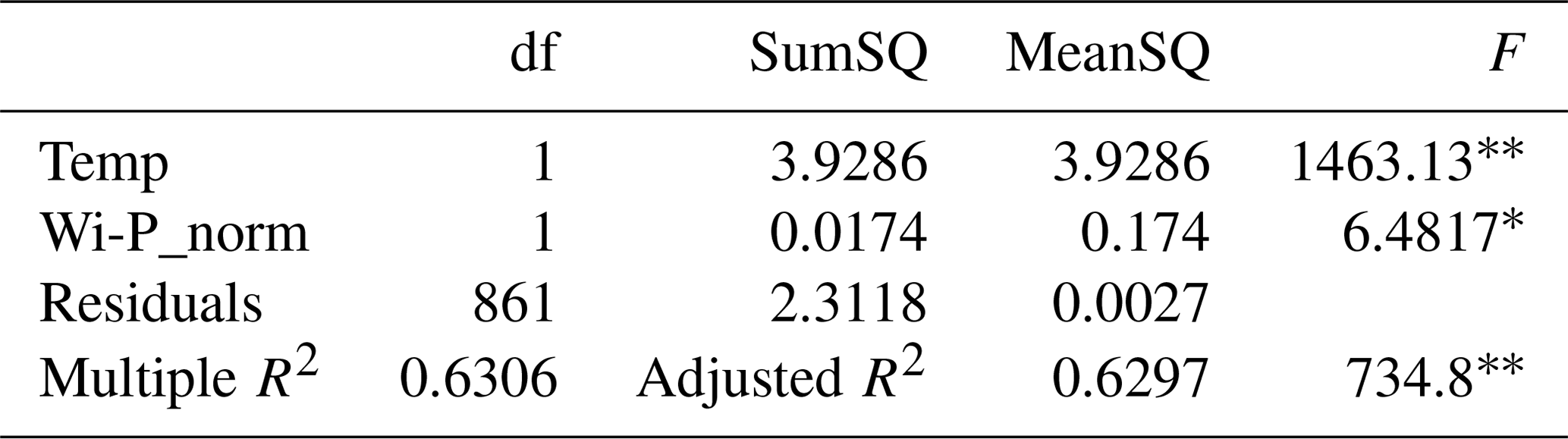
df: Degrees of Freedom. ^* p<0.05, ${}^{**}$ p<0.001.

Table 14 Parameter estimation in the regression model.

^* p<0.05, ${}^{**}$ p<0.001.

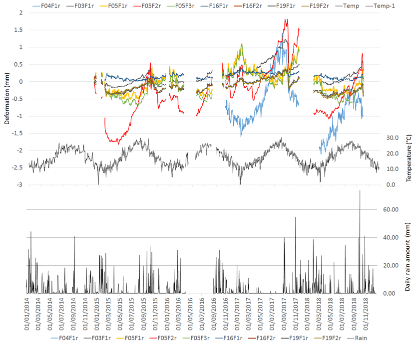
Figure 21 Comparison between crackmeter measurements, rain amount and daily temperature data time series.

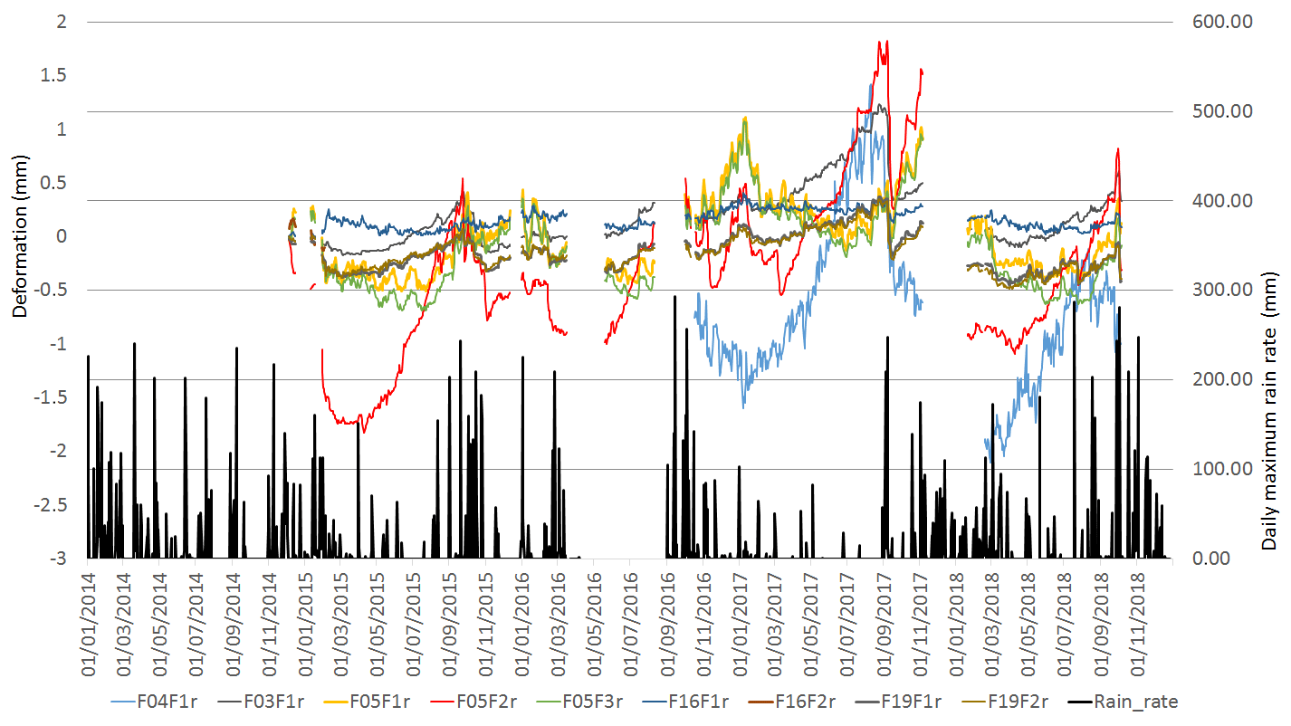
Figure 22 Comparison between crackmeter measurements and maximum daily rain rate data time series.

6 Discussion

Rock deformations involving five tuff blocks have been monitored for about 4 years (December 2014–October 2018) along the Coroglio coastal cliff, together with local meteorological parameters, whose measurements began in January 2014. The selected unstable tuff blocks, characterized by a volume of 4–15 m³, can be affected by toppling, planar and wedge sliding failure kinematics. The used sensors (nine monaxial crackmeters and two biaxial tiltmeters) captured several signs of tuff deformation through time as measured expansion and contraction of the fracture sheets and plane rotations above their accuracy (Table 2). Near-rock-surface air temperature (used as a proxy for surface rock temperature) and air temperature (together with other meteorological parameters) were measured by three thermistors on the cliff and a weather station installed at a distance of ∼1 km from the cliff. The whole dataset collected during the 5 years of monitoring activity has been described; the data distribution (Figs. 6, 8 and 9) and the temporal trends of the different parameters (Figs. 10 to 20) have been analyzed.

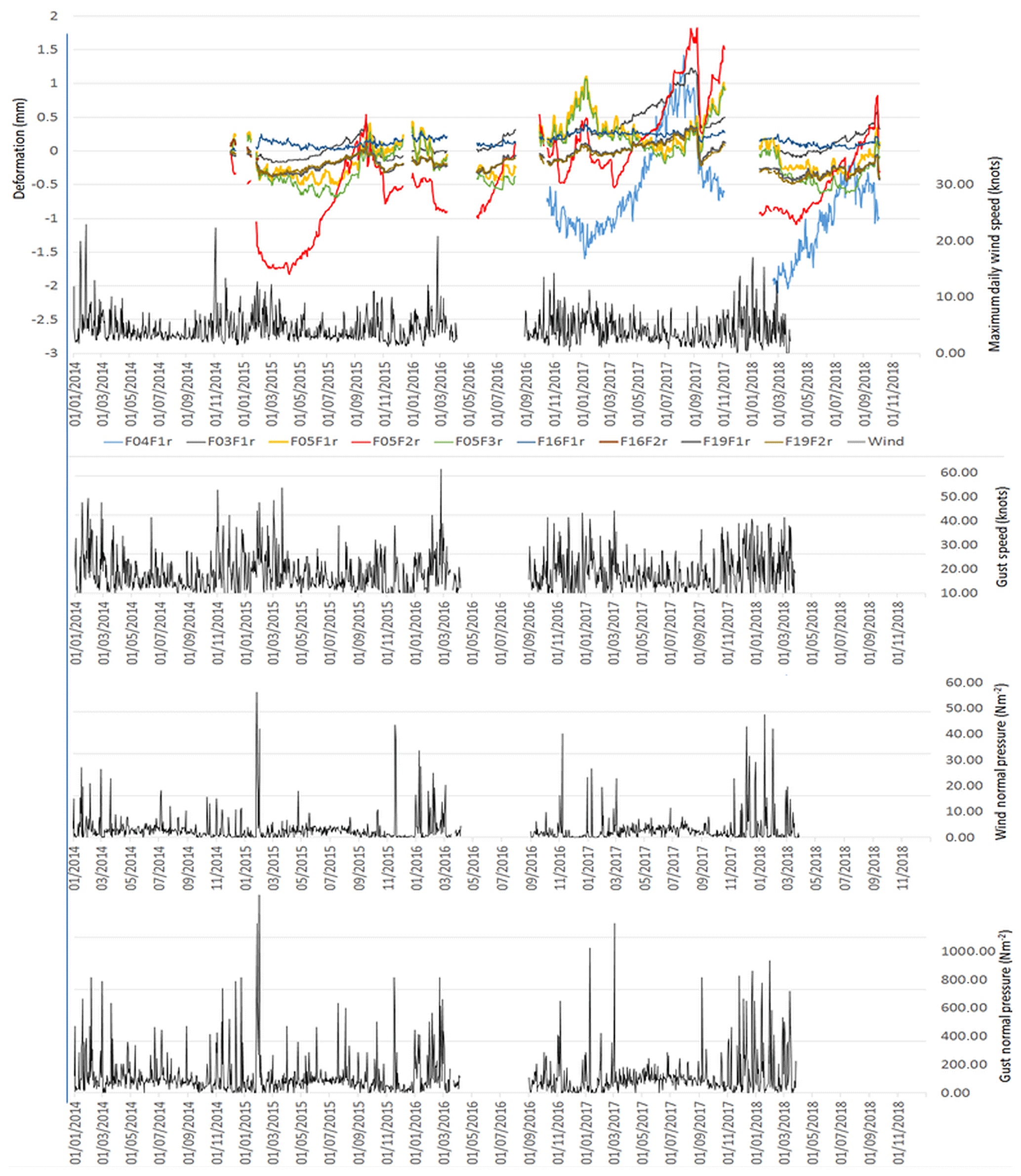
Figure 23 Comparison between crackmeter measurements and daily wind (wind speed, gust speed, wind normal pressure, gust normal pressure) data time series.

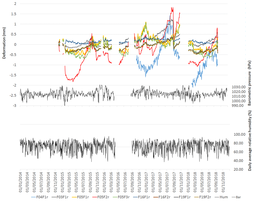
Figure 24 Comparison between crackmeter measurements, relative humidity and daily barometric pressure) data time series.

Based on a multivariate statistical analysis, we have recognized the relations between daily average values of tuff deformations and meteorological variables. Several positive correlations exist among rock deformation parameters and temperature data (Table 12). Positive correlations increase if we introduce a time lag of 2 to 5 weeks for temperature variables (Table 13), suggesting that there is a delayed time effect between thermal oscillations and rock deformations. In some cases, the tuff deformation is negatively correlated to wind pressure intensity acting on the cliff (e.g., F16F2). The regression analysis shows that if temperature and wind effect increase by one unit, deformation increases by 0.0114 and 0.0008, respectively. The coefficients of the model are significantly different from zero as the p values show.

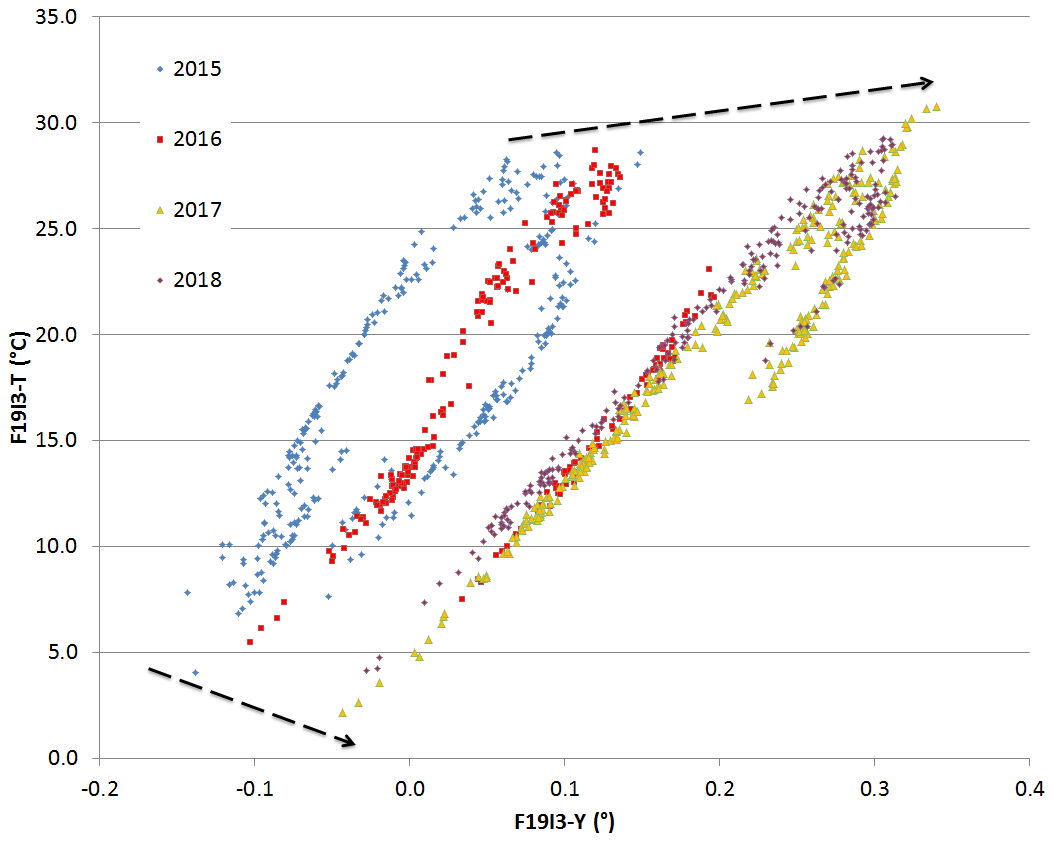
Figure 25 Progressive increase in tiltmeter F19I3-Y measurement values (see dashed arrows) from 2015 to 2018 for local temperature.

The detected cyclic changes in opening of fractures and rock face rotations appear linked to seasonal and annual temperature variations (Fig. 21). Crack aperture data reveal a deformation pattern characterized by seasonal cyclical deformation trends with strong temporal temperature coupling. In detail, when maximum temperatures level out (July–August), deformation continues to increase up to 30–40 d and reaches the maximum values during late August–September, each year. Minimum deformation values usually occur during winter–early spring (from January to April), after the seasonal cooling period. Some crackmeters show secondary peaks during the autumn–winter period, uncorrelated to temperature variation.

Similarly, we found comparatively little influence between rain and wind with the fracture deformation (Figs. 21–23). The rain seems to cause only sudden decreases in fracture opening during intense rainstorms (see events around 27 January 2015, 27 October 2015, 27 August 2017 and 27 September 2017; Figs. 21–22). Conversely, humidity and barometric pressure seem to exert no influence on fracture deformation (Fig. 24).

The temperature exerts the dominant role in driving daily average values of deformation, as the fracture deforms both synchronously and in a delayed way with temperature. Deformation of rocks measured by crackmeter sensors is partly linked to the bulk volume variation in the tuff, as a response to temperature changes. Tiltmeter measurements are also strongly forced by temperature annual cycles showing a cumulate increase from 2015 to 2018 (Fig. 25).

The direct result of heating rock is expansion, a process well studied and quantified in several environmental conditions (Chau and Shao, 2006; Collins and Stock, 2016; Eppes, 2016; Richter and Simmons, 1974). Cumulative fracture growth and opening can occur under typical present-day meteorological conditions in many settings (Eppes and Keanini, 2017; Lamp et al., 2017). Several diurnal and seasonal cycles of heating and cooling may lead to deformation and crack opening and propagation. Both increasing temperature and temperature fluctuations may also produce and enhance fracturing.

On a seasonal cycle, cumulative positive deformation peaks occur during the warmest months (June throughout September) yielding values up to 4 mm higher than the maximum negative deformation occurring during the coolest months (December through March; Fig. 21). This suggests that some rockfalls might be more likely during hot summer months, when crack sheets are at their maximum opening along the cliffs. Nevertheless, fracture opening is known to be a nonlinear process (Lawn, 1993), so we cannot simply use our measured deformation rates to predict future detachments of fracture sheets.

Our results have important implications for the triggering of rockfalls in cliffed landscapes. In fact, our measurements indicate that seemingly static tuffaceous landscapes are actually dynamic slopes. Along the Coroglio cliff, tuff blocks can deform in and out of a near-vertical cliff face by up to 1 mm on a daily basis and up to 4 mm on an annual scale. These data demonstrate the inherent instability of studied tuff cliffs as well as other rocky cliffs worldwide (Collins and Stock, 2016), mainly during summertime (Ishikawa et al., 2004; Gunzburger et al., 2005; Hasler et al., 2012; Vargas et al., 2012; Stock et al., 2013; Collins and Stock, 2016).

7 Data availability

The databases presented and discussed in this article are available for download from the PANGAEA Repository. Deformation and meteorological datasets are respectively provided in separated files in tab format at: https://doi.org/10.1594/PANGAEA.896000 (Matano et al., 2018) (deformation data with frequency sampling of 30 min) and at: https://doi.org/10.1594/PANGAEA.899562 (Fortelli et al., 2019) (meteorological data with frequency sampling of 10 min).

8 Conclusions

The Coroglio cliff shares broad characteristics with several tuff cliffs from the Phlegraean Fields coastal area affected by severe retreat processes, and elsewhere in the world. In our research, we have focused on in situ measurements of deformations affecting tuff blocks. The CC-MoSys, installed in December 2014, has captured some of the tuff deformation behavior under the different meteorological conditions that occurred during about 5 years. Our results indicate that seemingly static tuffaceous landscapes are quite dynamic cliffs.

The data recorded by the Coroglio cliff monitoring system have contributed to our understanding of temperature–tuff deformation relationships in the analyzed cliff. Micro-deformation of rocks measured by geotechnical sensors reveals a general cyclic trend, possibly linked to the bulk volume variation in the rocks, as a response to seasonal and daily temperature variations. On an annual cycle, the cumulative positive deformation peaks occurring during summertime may yield values up to 1 to 4 mm higher than the most negative deformation occurring during wintertime.

More in general, this research provides a first contribution to the knowledge about the generation of tuff block instability phenomena and the understanding of the rates of geomorphic evolution of a coastal tuff cliff. The analysis of the relationships between deformation and meteo-marine forcing factors may also be very useful in the perspective of early-warning actions and policies, also due to the location of the study site in a densely urbanized area.