the Creative Commons Attribution 4.0 License.
the Creative Commons Attribution 4.0 License.
 | 16 Oct 2020
Apparent ecosystem carbon turnover time: uncertainties and robust features
Sujan Koirala
Markus Reichstein
Martin Thurner
Valerio Avitabile
Maurizio Santoro
Bernhard Ahrens
Ulrich Weber
The turnover time of terrestrial ecosystem carbon is an emergent ecosystem property that quantifies the strength of land surface on the global carbon cycle–climate feedback. However, observation- and modeling-based estimates of carbon turnover and its response to climate are still characterized by large uncertainties. In this study, by assessing the apparent whole ecosystem carbon turnover times (τ) as the ratio between carbon stocks and fluxes, we provide an update of this ecosystem level diagnostic and its associated uncertainties in high spatial resolution (0.083∘) using multiple, state-of-the-art, observation-based datasets of soil organic carbon stock (Csoil), vegetation biomass (Cveg) and gross primary productivity (GPP). Using this new ensemble of data, we estimated the global median τ to be yr () when the full soil is considered, in contrast to limiting it to 1 m depth. Only considering the top 1 m of soil carbon in circumpolar regions (assuming maximum active layer depth is up to 1 m) yields a global median τ of yr, which is longer than the previous estimates of yr (Carvalhais et al., 2014). We show that the difference is mostly attributed to changes in global Csoil estimates. Csoil accounts for approximately 84 % of the total uncertainty in global τ estimates; GPP also contributes significantly (15 %), whereas Cveg contributes only marginally (less than 1 %) to the total uncertainty. The high uncertainty in Csoil is reflected in the large range across state-of-the-art data products, in which full-depth Csoil spans between 3362 and 4792 PgC. The uncertainty is especially high in circumpolar regions with an uncertainty of 50 % and a low spatial correlation between the different datasets () when compared to other regions (). These uncertainties cast a shadow on current global estimates of τ in circumpolar regions, for which further geographical representativeness and clarification on variations in Csoil with soil depth are needed. Different GPP estimates contribute significantly to the uncertainties of τ mainly in semiarid and arid regions, whereas Cveg causes the uncertainties of τ in the subtropics and tropics. In spite of the large uncertainties, our findings reveal that the latitudinal gradients of τ are consistent across different datasets and soil depths. The current results show a strong ensemble agreement on the negative correlation between τ and temperature along latitude that is stronger in temperate zones (30–60∘ N) than in the subtropical and tropical zones (30∘ S–30∘ N). Additionally, while the strength of the τ–precipitation correlation was dependent on the Csoil data source, the latitudinal gradients also agree among different ensemble members. Overall, and despite the large variation in τ, we identified robust features in the spatial patterns of τ that emerge beyond the differences stemming from the data-driven estimates of Csoil, Cveg and GPP. These robust patterns, and associated uncertainties, can be used to infer τ–climate relationships and for constraining contemporaneous behavior of Earth system models (ESMs), which could contribute to uncertainty reductions in future projections of the carbon cycle–climate feedback. The dataset of τ is openly available at https://doi.org/10.17871/bgitau.201911 (Fan et al., 2019).
- Article
(8258 KB) - Full-text XML
-
Supplement
(4323 KB) - BibTeX
- EndNote


Terrestrial ecosystem carbon turnover time (τ) is the average time that carbon atoms spend in terrestrial ecosystems from the initial photosynthetic fixation until respiratory or non-respiratory loss (Bolin and Rodhe, 1973; Barrett, 2002; Carvalhais et al., 2014). Ecosystem turnover time is an emergent property that represents the macro-scale turnover rate of terrestrial carbon that results from different processes such as plant mortality and soil decomposition. Alongside photosynthetic fixation of carbon, τ is a critical ecosystem property that co-determines the terrestrial carbon storage and the terrestrial carbon sink potential. The magnitude of τ and its sensitivity to climate change are central to modeling carbon cycle dynamics. Therefore, τ has been used as a model evaluation diagnostic and to constrain Earth system model (ESM) simulations of the carbon cycle. These analyses have shown that current ensembles of ESMs show a large spread in the simulation of soil and vegetation carbon stocks and their spatial distribution, which are mostly attributed to the differences in τ among ESMs (Friend et al., 2014; Todd-Brown, 2013, 2014; Wenzel et al., 2014, Carvalhais et al., 2014; Thurner et al., 2017).
At large scales, and for ecosystem-level comparisons, model simulations and observations do not agree in the global distribution of τ and its relationship with climate. Previous observational datasets, covering both lower latitudes and circumpolar regions and used to estimate global τ for comparison with ESM simulations from the fifth phase of the Coupled Model Intercomparison Project (CMIP5) have shown a generalized tendency of the models towards faster turnover times of carbon which are more sensitive to temperature when compared to observation-based estimates (Carvalhais et al., 2014). The variability between the ESMs alone was also substantial, showing a wide range of τ from 8.5 to 22.7 yr (mean difference of 29 %) leading to a substantial divergence in global simulated total terrestrial carbon stocks that range from 1101 to 3374 PgC (mean difference of 36 %). The models also exhibit a large discrepancy in the τ–temperature and τ–precipitation relationships across different latitudes compared to observations. The difficulty of evaluating the response of soil carbon to climate change is partly due to the fact that the dynamical observations at relevant timescales, e.g., multi-decadal to centennial scales, are lacking, and the magnitude of projected change in τ to climate change is still poorly constrained (Koven et al., 2017).
The current understanding of the factors that drive changes in τ is unclear due to the confounding effects of temperature and moisture even though, for instance, it is well perceived that temperature and water availability are the main climate factors that affect root respiration and microbial decomposition (Raich and Schlesinger, 1992; Davidson and Janssens, 2006; Jackson et al., 2017). Therefore, it is difficult to implement the local temperature sensitivity of τ into carbon cycle models due to the large discrepancy between the intrinsic and apparent sensitivity of τ to temperature. As the soil environment and climate are highly heterogeneous in space, the temperature sensitivity of τ and terrestrial carbon fluxes may be substantially affected by other factors as spatial scale decreases (Jung et al., 2017). Additional challenges emerge in understanding the role of climate and other environmental factors in defining vegetation dynamics related to mortality and recovery trajectories that control the plant-level contribution to τ (Friend et al., 2014; Thurner et al., 2016). Large uncertainties in the simulated total carbon stock of soil and vegetation represent process uncertainty or potentially missing processes that lead to diverse or even opposite responses of τ to changes in climate (Friedlingstein et al., 2006; Friend et al., 2014). Thus, it is instrumental to use observation-based estimations of carbon turnover times and their associated uncertainties in order to constrain the models and better predict the response of the carbon cycle to climate change.
On the other hand, the observation-based estimates of carbon turnover times themselves are prone to uncertainties stemming from the different data sources of different components of τ: soil and vegetation stocks and ecosystem carbon flux. Specifically, estimates of global total carbon stocks are characterized by large uncertainties because different in situ measurements and upscaling methods are used to derive total carbon stocks (Batjes, 2016; Hengl et al., 2017; Sanderman et al., 2017). Alongside recent soil carbon datasets (Tifafi et al., 2018), there are also several different global vegetation biomass estimates (Thurner et al., 2014; Avitabile et al., 2016; Sassan Saatchi, personal communication, 2011; Santoro et al., 2020) and gross primary productivity (GPP) datasets (Jung et al., 2017), which may lead to substantial differences in the global τ distribution and its relationship with climate. Thus, building and evaluating an observation-based ensemble of global τ estimates derived from different products is key in quantifying the uncertainties in the τ–climate relationship.
This study thus aims at developing an ensemble global estimation of τ at a spatial resolution of 0.083∘, which is derived from different observation-based products. Specifically, we will (1) update τ estimations with multiple state-of-the-art datasets, (2) quantify the contribution of the different components of τ to the global and local uncertainties, and (3) identify the robust patterns across the different ensemble members.
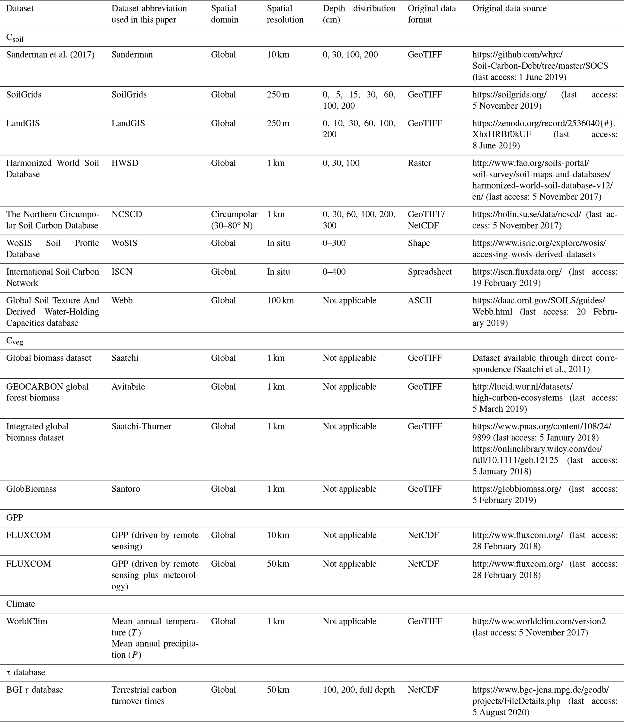
The attributes of the τ dataset provided in this study and the key external datasets that were used to estimate τ are summarized in Table 1. Details for each dataset are described in the following subsections. Note that all the datasets are harmonized into the same spatial resolution of 0.083∘ (∼10 km) using a mass conservative approach (see Sect. S1 in the Supplement).
2.1 Soil organic carbon datasets
Five different estimates of global soil carbon stock (Csoil) were obtained from independent datasets. The main features of the datasets and the approaches used are briefly described below:
- a.
SoilGrids is an automated soil mapping system that provides consistent spatial predictions of soil properties and types at the spatial resolution of 250 m (Hengl et al., 2017). A global compilation of in situ soil profile measurements is used to produce an automated soil mapping based on machine learning algorithms. The dataset contains global soil organic carbon content at soil depths of 0, 5, 15, 30, 60, 100 and 200 cm. In addition, physical and chemical soil properties such as bulk density and carbon concentration are provided. A total of 158 remote-sensing-based covariates including land cover classes and long-term averaged surface temperature were used to train the machine learning model at the site level. According to Hengl et al. (2017), the current version of the dataset explains 68.8 % of the variance in soil carbon stock compared to a mere 22.9 % in the previous version (Hengl et al., 2014). However, it has also been recognized that SoilGrids may overestimate carbon stocks due to high values of bulk soil density (Tifafi et al., 2018). In general, the estimation of Csoil is mainly caused by the geographically biased availability of measured data especially in the circumpolar regions. Even though in situ measurements had a large spatial extent and cover most of the continents, the remote regions that are characterized by severe climate were sampled much less.
- b.
The dataset of soil carbon provided by Sanderman et al. (2017; hereafter Sanderman) used the same method as SoilGrids but different input covariates. The main difference between SoilGrids and Sanderman is that, in addition to topographic, lithological and climatic covariates, Sanderman also included land use and forest fraction as covariates in the model fitting. The relative importance analysis based on the random forest method showed that soil depth, temperature, elevation and topography are the most important predictors of soil carbon, which is consistent with SoilGrids. Land use types such as grazing and cropland also contribute significantly to the variance. The Sanderman dataset provides soil carbon stocks for the soil depths of 0–30, 30–100 and 100–200 cm. The dataset is available at a spatial resolution of 10 km.
- c.
The Harmonized World Soil Database (HWSD) coordinated soil data from more than 16 000 standardized soil-mapping units worldwide into a global soil dataset (Batjes, 2016). It combines regional and national soil information to estimate soil properties, and yet reliability of the data varies due to the different data sources. The database derived from the SOTER soil and terrain database had the highest reliability (Central and Eastern Europe, the Caribbean, Latin America, southern and eastern Africa), while the database derived from the Soil Map of the World (North America, Australia, western Africa and South Asia) had a relatively lower reliability. The HWSD dataset is available at a spatial resolution of 30 arc seconds, and it includes soil organic carbon and water storage capacity at topsoil (0–30 cm) and subsoil (30–100 cm).
- d.
The Northern Circumpolar Soil Carbon Database (NCSCD) quantifies the soil organic carbon storage in the northern circumpolar permafrost area (Hugelius et al., 2013). The dataset contains soil organic carbon content for soil depths of 0–30, 0–100, 100–200 and 200–300 cm. The soil samplings included pedons from published literature, existing datasets and unpublished material. The data for 200 and 300 cm depths were obtained by extrapolating the bulk density and carbon content values at the deepest available soil depth for a specific pedon. Only the pedons with the data for at least the first 50 cm were extrapolated to the full soil depth. The deep soil carbon (100–300 cm) showed the lowest level of confidence due to lack of in situ measurements and much lower spatial representativeness.
- e.
The soil carbon stock and properties produced by the LandGIS maps development team (hereafter LandGIS) were also used in this study (Wheeler and Hengl, 2018). The soil profile measurements used in the training have a wide geographic coverage in America, Europe, Africa and Asia. One unique feature of LandGIS is that it includes additional soil profiles in Russia from the Dokuchaev Soil Science Institute and the Russian Ministry of Agriculture, improving the predictions of Csoil significantly there. Further, different machine learning methods, including random forest, gradient boosting and multinomial logistic regression, were used to upscale the soil profiles to a global gridded dataset. Continuous soil properties were predicted at six different soil depths: 0, 10, 30, 60, 100 and 200 cm. Compared to the SoilGrids dataset, LandGIS added new remote sensing layers as covariates in the training and used 5 times more training datasets (360 000 soil profiles compared to 70 000 in SoilGrids).
2.2 Vegetation biomass datasets
Four different datasets of biomass were used to produce the total vegetation biomass (Cveg) data on the global scale.
- a.
Thurner et al. (2014) estimated the aboveground biomass (AGB) and belowground biomass (BGB) for Northern Hemisphere boreal and temperate forests based on satellite radar remote sensing retrievals of growing stock volume (GSV) and field measurements of wood density and biomass allometry. The carbon stocks of tree stems were estimated from GSV retrieval of the BIOMASAR algorithm. The BIOMASAR algorithm uses remote sensing observations from the Advanced Synthetic Aperture Radar (ASAR) instrument on the Envisat satellite (Santoro et al., 2015). The remote sensing retrievals are then converted to biomass using information on wood density and allometry. The other tree biomass compartments (BCs) including roots, foliage and branches were estimated from stem biomass using field measurements of biomass allometry. The total carbon content of the vegetation was then derived as the sum of the biomass in different compartments and converted to carbon mass units using carbon fraction parameters. A comparison between the data and inventory-based estimates shows good agreement on regional scales in Russia, the United States and Europe (Thurner et al., 2014). The data from Thurner et al. (2014), at 0.01∘ spatial resolution and representative for the year 2010, only cover the northern boreal and temperate forests between 30∘ and 80∘ N latitudes.
- b.
To accommodate for lower latitudes not covered in the Thurner et al. (2014) data, we used the forest biomass carbon stocks to cover the tropical regions provided by Saatchi et al. (2011). The data were derived using lidar, optical and microwave satellite imagery trained with in situ measurements in 4079 forest inventory plots (Saatchi et al., 2011). Using the Geoscience Laser Altimeter System (GLAS) lidar observations to sample forest structure, the method applies a power-law functional relationship to estimate biomass from the lidar-derived Lorey's height of the canopy. This extended sample of biomass density is then extrapolated over the landscape using MODIS and radar imagery, resulting in a pantropical AGB map. BGB was estimated as a function of AGB, and the two were summed together to derive total forest carbon stock at 1 km spatial resolution.
- c.
The GlobBiomass map (Santoro et al., 2018) estimated GSV and AGB density on the global scale for the year 2010 at 100 m spatial resolution. The AGB was derived from GSV using spatially explicit biomass conversion and expansion factors (BCEFs) obtained from an extensive dataset of wood density and compartment biomass measurements. GSV was estimated using space-borne synthetic aperture radar (SAR) imagery (the Advanced Land Observing Satellite's Phased Array type L-band Synthetic Aperture Radar – ALOS PALSAR – and Envisat's ASAR), Landsat-7, ICESat's lidar and auxiliary datasets and utilizing the BIOMASAR algorithm to relate the SAR backscattered intensity with GSV (Santoro et al., 2018).
- d.
Avitabile et al. (2016) combined two existing AGB datasets (Saatchi et al., 2011; Baccini et al., 2012) to produce data for pantropical AGB. These data use a large independent reference biomass dataset to calibrate and optimally combine the two maps. The data fusion approach is based on the bias removal and weighted-average of the input maps, which integrates the spatial patterns of the reference data into the combined data. The resulting data of total AGB stock for the tropical regions were 9 %–18 % lower than the two reference datasets with distinctive spatial patterns over large areas. The combined data from Avitabile et al. (2016) is available at a spatial resolution of 1 km.
2.3 Soil depth dataset
The data for global distribution of soil depth were obtained from the Global Soil Texture and Derived Water-Holding Capacities database (Webb et al., 2000). The data contain standardized values of soil depth and texture selected from the values from the same soil type within each continent. The total soil depth depends on soil texture and water availability, and it is usually deeper than 100 cm. In regions with permafrost, total soil depth can extend beyond 400 cm (Fig. S1 in the Supplement).
2.4 Gross primary productivity datasets
The GPP datasets used to calculate ecosystem carbon turnover times were obtained from the FLUXCOM initiative (http://fluxcom.org/, last access: 28 February 2018). In FLUXCOM, the global energy and carbon fluxes are upscaled from eddy covariance flux measurements using different machine learning approaches with meteorological and Earth observation data (Jung et al., 2017). In this study, we used GPP derived from the two different FLUXCOM setups based on (1) only remote sensing covariates and (2) both remote sensing and meteorology forcing (Tramontana et al., 2016; Jung et al., 2020). In this study, we derived the long-term mean annual GPP across different machine learning methods over the time period from 2001 to 2015.
2.5 Climate datasets
The high spatial resolution (∼1 km) climate dataset WorldClim (Fick and Hijmans, 2017) was used to investigate the relationship between τ and climate. The data included monthly maximum, minimum, and average temperature, precipitation, solar radiation, vapor pressure, and wind speed. The WorldClim data were produced by assimilating 9000–60 000 ground-station measurements and covariates such as topography, distance to the coast and remote sensing satellite products including maximum and minimum land surface temperature, as well as cloud cover in model fitting. For different regions and climate variables, different combinations of covariates were used. The 2-fold cross-validation statistics showed a very high model accuracy for temperature-related variables (r>0.99) and a moderately high accuracy for precipitation (r=0.86).
3.1 Estimation of ecosystem turnover times
As a result of the balance between influx and outflux of carbon, the terrestrial carbon pool can be approximated to reach the steady-state condition (influx equals outflux) when long timescales are considered. This simplifies the calculation of τ to the ratio between the total terrestrial carbon storage and the influx or the outflux of carbon. The approach is advantageous in representing the highly heterogeneous intrinsic properties of the terrestrial carbon cycle as an averaged apparent ecosystem property which is more intuitive to infer large-scale sensitivity of τ to climate change. Instead of focusing on the heterogeneity of individual compartment turnover times, we show the change in the carbon cycle on the ecosystem level using τ as an emergent diagnostic property. The total land carbon storage can be estimated by summing soil carbon stocks derived from extrapolation and vegetation biomass. Assuming a steady state in which the total efflux (autotrophic and heterotrophic respiration, fire, etc.) equals the influx (GPP), then τ can be calculated as the ratio between carbon stock and influx:
where Csoil and Cveg are the total soil and vegetation carbon stocks, respectively, and GPP is the total influx to the ecosystem. An ensemble of τ estimates is generated by combining three soil carbon stocks at three different soil depths (1 m, 2 m, full soil depth), four vegetation biomass products, and 24 GPP values resulting in an ensemble with 864 members.
3.2 Estimation of global vegetation biomass stock
Two different corrections had to be addressed in order to assess the whole vegetation carbon stock from current observation-based products. First, the aboveground biomass datasets only consider the biomass within woody vegetation (mostly trees), while the biomass of herbaceous vegetation is missing. To account for herbaceous biomass, we used a previously developed method in which the live vegetation fraction is assumed to have a mean turnover time of 1 yr and a uniform distribution of respiratory costs of carbon (Carvalhais et al., 2014). The carbon in herbaceous vegetation can then be expressed as a function of GPP:
where CH is the carbon stock of the herbaceous vegetation, GPP is the gross primary productivity from FLUXCOM, α is respiration cost of carbon (0.25–0.75), and fH is the fraction of a grid cell covered by herbaceous vegetation, which was obtained from the SYNMAP database (Jung et al., 2006).
Second, two of the vegetation biomass datasets (GlobBiomass and Avitabile; see Table 1) do not include BGB. For consistency across all Cveg datasets, we estimated the BGB using a previously developed empirical relationship (Saatchi et al., 2011) between AGB and BGB:
3.3 Extrapolation of soil datasets
We used observed soil profiles and multiple empirical models to extrapolate soil carbon stock to full soil depth (Fig. S1 and Table S1 in the Supplement). This approach is necessary to obtain the accumulated carbon stock from the surface to full soil depth because the soil datasets only extend up to 2 m below the surface. However, a large amount of Csoil is stored below this depth, especially in peatland regions where soil carbon content can be substantially higher in deeper soil layers (Hugelius et al., 2013). To estimate the total carbon storage in the land ecosystem, different empirical mathematical models were used (Table S1 in the Supplement). The covariance matrix adaptation evolution strategy (CMA-ES) method, which is based on an evolutionary algorithm that uses the pool of stochastically generated parameters of a model as the parents for the next generation (Hansen et al., 2001), was used to optimize parameters of the models.
Extrapolation using empirical numerical models may cause arbitrary bias and higher uncertainty if the models are not appropriately chosen. Here we used the in situ observational data from the World Soil Information Service (WOSIS) (Batjes et al., 2020) and the International Soil Carbon Network (ISCN) (Nave et al., 2017) to select the ensemble of the models that could best simulate soil carbon stocks at full depth. We used a global dataset of soil depth (Webb, 2000) as the maximum soil depth to which we extrapolated. The approach fit each empirical model against cumulative Csoil with all data points and then predicted the cumulative Csoil at full soil depth for each soil profile independently. The ability of a particular empirical model or combination of models was then evaluated by comparing the predictions of Csoil at full depth against the observations (see Sect. S3.2 in the Supplement). This procedure was applied to the two different in situ datasets: WOSIS, which covers most of the biomes, and ISCN, which has more coverage in circumpolar regions. Finally, after comparing different model averaging methods (see Table S2 in the Supplement), we chose two model ensembles that could best represent circumpolar and non-circumpolar regions based on observational datasets. The performance of the chosen ensembles is synthesized in Figs. S3 and S4 in the Supplement. Finally, each model ensemble is applied to extrapolate Csoil to full depth in corresponding regions (see Sect. S3 in the Supplement).
3.4 Uncertainty estimation
To estimate the sources of uncertainty in τ, we performed an n-way analysis of variance (ANOVA) on the different variables (Csoil, Cveg and GPP). The ANOVA provides the sum of squares of each variable and the total sum of squares of all variables. The contribution of each variable (data from different sources) to the total uncertainty can then be calculated as follows:
where Cn is the relative contribution of uncertainty from the nth variable, SSn is the sum of the square of the nth variable, and SStotal is the total sum of the square of all variables. Note that the uncertainty was quantified in two domains:
-
grid cell – the relative contributions of different variables to uncertainty in τ were calculated independently for each grid cell;
-
global – the same method was applied to the estimate of the global τ, which is calculated using the global total carbon stocks in vegetation and soil and GPP.
3.5 The analysis of zonal correlations
The local correlation between τ and climate across latitudes was obtained by using a zonal moving window approach in which the Pearson partial correlations between τ and T and P were calculated using a 360∘ (longitudinal span) × 2.5∘ (latitudinal span) moving window. This approach allowed for the assessment of the correlation strength between τ and each climate parameter. The τ values below the local 1st percentile and above the 99th percentile were removed in each moving window to avoid the effect of potential outliers in the correlations with climate. In order to investigate the effect of latitudinal span, we chose different band sizes of 0.5∘, 2.5∘ and 5∘ and performed the correlation analysis in the same manner for each selection.
4.1 The global carbon stock
Table 2 summarizes the estimates of Csoil, Cveg and GPP. Globally, estimates of soil carbon stocks within the top 2 m of soil are 2863, 3969 and 3710 PgC for the datasets of Sanderman, SoilGrids and LandGIS, respectively (bulk density corrected; see Sect. S2 in the Supplement). The significant differences among different datasets indicate a high uncertainty in the current estimation of global soil carbon storage. The extrapolation of Csoil to the full soil depth (FD) shows that approximately 18 % of soil carbon is stored below the depth of 2 m. Compared to the previous generation of HWSD Csoil data (available only for top 1 m), the current state-of-the-art datasets show significantly higher Csoil within the top 1 m (Table 2). On the other hand, the current datasets of vegetation biomass show global Cveg ranges from 392 to 437 PgC and substantially lower relative uncertainty than Csoil. The estimation of the uncertainty that is derived from different GPP members shows a range of 100 to 123 PgC (10th percentile to 90th percentile) from different products. Note that the GPP members are different realizations from FLUXCOM and encompass a wide range of sources of uncertainty such as different climate forcing, use of remotely sensed data and machine learning methods (see Sect. 2.4). Overall, the results show that the differences in Csoil estimates are substantially larger than the differences in Cveg and GPP datasets.
Table 2Estimates of soil organic carbon stocks (PgC), vegetation biomass (PgC) and GPP (PgC yr−1).

n/a: not applicable
4.2 The spatial distribution of soil carbon stocks
A significant amount of soil organic carbon is stored in high-latitude terrestrial ecosystems, especially in the permafrost regions (Hugelius et al., 2013). However, in comparison with low latitudes, the uncertainties of Csoil distribution and storage in high latitudes are potentially higher due to fewer available observations of soil profiles. We therefore divided the global soil carbon into the non-circumpolar (Fig. 1) and the circumpolar (Fig. 2) regions based on the northern permafrost region map of the NCSCD. The results show that the mean value and range (maximum–minimum) of Csoil in non-circumpolar regions (Table 2) in the top 2 m are 2136 and 537 PgC and in the circumpolar regions within the top 2 m are 1278 and 574 PgC.
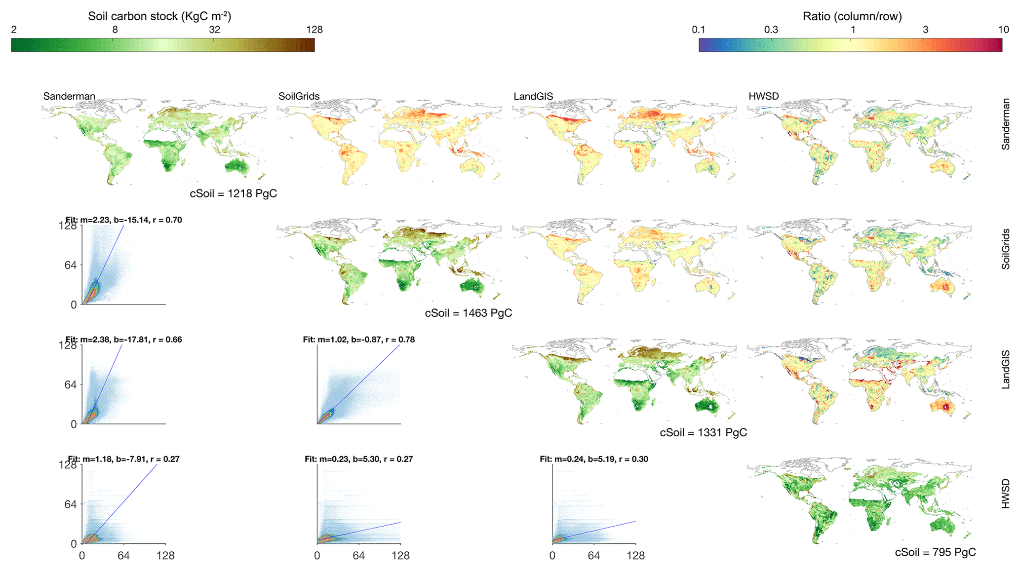
Figure 1Spatial distributions of soil carbon storage at 0–100 cm in the non-circumpolar regions. The total amount of carbon stock is shown in the bottom of each diagonal panel. The upper off-diagonal panels show the ratios between each pair of datasets (column/row). The bottom off-diagonal panels show the density plots and major axis regression line between each pair of datasets (m: slope, b: intercept, r: correlation coefficient). The ranges of both of the color bars approximately span between the 1st and the 99th percentiles of the data. Hereafter, all figures comparing different spatial maps include the information in a similar manner.
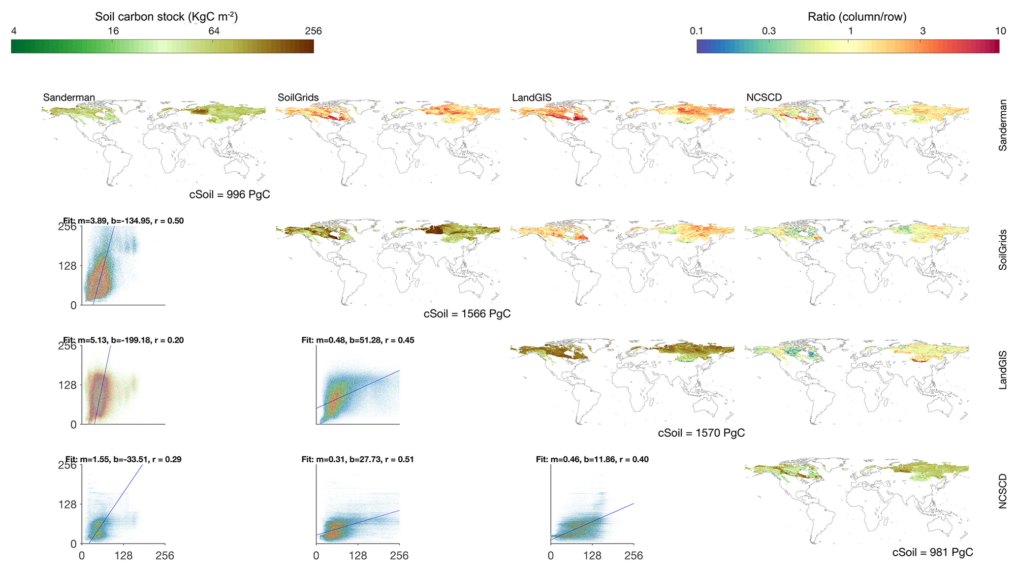
Figure 2The same as Fig. 1 except for the Csoil in 0–200 cm soil depth and in the circumpolar regions.
We used in situ observed soil profiles (Fig. S1 in the Supplement) and multiple empirical models to select an ensemble of models to extrapolate soil carbon stock to full soil depth (Fig. S2 and Table S1 in the Supplement). It was apparent that a unique ensemble would be limited to represent Csoil profiles globally, resulting in two different model ensembles being selected to represent the soil vertical distribution: one for the circumpolar regions, and another for non-circumpolar regions. In general, the results show good model performances for predicting in situ soil carbon stocks up to full soil depth, although non-circumpolar regions (Fig. S3 in the Supplement) show a higher model performance than that in circumpolar regions (Fig. S4 in the Supplement). The global estimation of Csoil to full soil depth results in a higher mean value of 2678 PgC in non-circumpolar regions and 1637 PgC in circumpolar regions. Our results show that there are approximately 500 and 400 PgC of carbon stock stored in the deep soil layer below 2 m in non-circumpolar and circumpolar regions, respectively.
The spatial distribution of Csoil is more consistent across datasets in the non-circumpolar regions than in the circumpolar regions (Fig. 1). The Pearson correlation coefficients (r) between each pair of datasets in the non-circumpolar regions are generally higher than in the circumpolar regions. Our results show a moderate agreement among the datasets in the spatial distribution of Csoil globally (r>0.65). However, there are significant differences in the spatial patterns between the HWSD and each dataset (Fig. 1) as the correlation coefficients are all below 0.3. In addition, there is a 2-fold lower carbon storage in the HWSD than the other datasets. Ratios between the total Csoil in the top 100 cm (Fig. 1, upper off diagonal plots) show that LandGIS, SoilGrids and Sanderman are consistent in temperate regions but show poor agreement in the tropical and the boreal regions. The comparison also shows that the gradient in carbon stocks between Europe and the lower latitudes diminished in the HWSD soil map. In addition, the spatial distribution and the amount of carbon stocks in insular Southeast Asia are significantly different in the HWSD.
Greater dissimilarities of spatial patterns across the datasets in the circumpolar regions are shown in Fig. 2. We included the NCSCD dataset which specifically focuses on the circumpolar regions. The spatial correlations between each pair of the four datasets show low correlation values (r) which range from 0.2 to 0.5. In contrast to the non-circumpolar regions, the high spatial dissimilarity in circumpolar regions indicates higher uncertainty regarding the estimation of total carbon storage. However, there is no evidence on which dataset is more credible in terms of total carbon storage and spatial pattern. The large differences are possibly due to fewer observational soil profiles in the northern high-latitude regions, which are crucial in the model training process (Hugelius et al., 2013; Hengl et al., 2017).
The comparison between all datasets shows good agreement in the vertical structure of terrestrial carbon stocks. The Csoil in the top 1 m is about half of the total terrestrial carbon and 80 % of the top 2 m of Csoil regardless of region or data source. For the non-circumpolar regions, all the datasets show significantly higher carbon storage in the top 1 m than that in the HWSD while showing less divergence of carbon storage among these three datasets (Table 2). In general, the current datasets show a similar vertical distribution of Csoil with consistent values and ratios between 1 and 2 m soil. The extrapolation results indicate that about 20 % of carbon is stored below 2 m in the non-circumpolar regions. For the circumpolar regions, the four datasets show a clear trend that the difference of Csoil increases with soil depth, as shown in Table 2. The difference between the top 1 m of Csoil among datasets has a higher difference than that of 2 m. However, the ratio between storage in 1 and 2 m is similar across all datasets.
4.3 The spatial distribution of vegetation
Different from the spatial distribution of soil carbon, most vegetation carbon is stored in the tropics, whereas much less carbon resides in the higher latitudes. In fact, the Cveg in the circumpolar regions is only 10 % of that in the non-circumpolar regions (Table 2). In comparison with soil carbon, the results show higher consistency and convergence in global estimates of carbon stock among the four global vegetation datasets (Fig. 3). Our results show that the global vegetation carbon stock is 10 % to 25 % of the global soil carbon stock depending on the soil depth considered. The significant spatial correlations (r>0.75, α<0.01) between each of the estimates indicate a consistent global spatial distribution of vegetation across the different data sources. However, the results show more heterogeneity in the regional distribution of vegetation biomass and uncertainty of Cveg. Specifically, Cveg in arid and cold regions has higher relative uncertainty than that in the moist and hot regions.
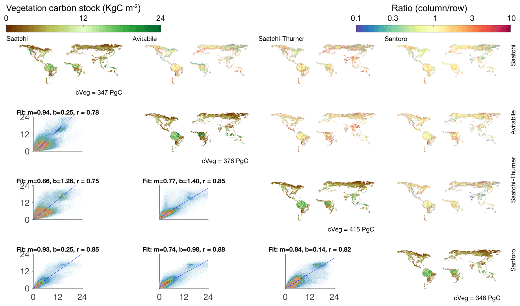
Figure 3The same as Fig. 1 but for vegetation carbon stocks. The total vegetation carbon stock is calculated as the sum of aboveground (AGB), belowground (BGB) and herbaceous biomass. For consistency, only the grid cells where all four maps have values are included. Therefore, the total amounts in the diagonal panels differ slightly from those in Table 2.
The Cveg consists of three components including AGB, BGB and herbaceous biomass. The herbaceous biomass is estimated from mean annual GPP (see Sect. 3.2; Carvalhais et al., 2014) and globally represents 5 % of the total Cveg and less than 1 % of the total Csoil, indicating the minor role of herbaceous biomass in affecting the global estimates and the spatial distribution of τ. The comparison among the four vegetation datasets shows a mean of 410 PgC in Cveg with a spread of 11 % across the different datasets and a consistent spatial distribution across the different sources. Locally these differences can be higher, as observed in the relatively higher level of disagreement in sparsely vegetated arid regions and some cold regions (Fig. 3, upper off-diagonal panels).
4.4 The spatial distribution of GPP
The global spatial distribution of GPP is similar to that of Cveg, i.e., high in the tropical regions and low in the higher latitudes (Fig. 4). The GPP datasets show high consistency in both the spatial patterns and global values. The spread in GPP estimates is higher (>50 %) in arid and polar regions than the other regions (Fig. 4, upper off-diagonal plots). Although the differences among different vegetation and GPP estimations, in general, are not as high as in soil carbon, the regionally high uncertainties can be significant.
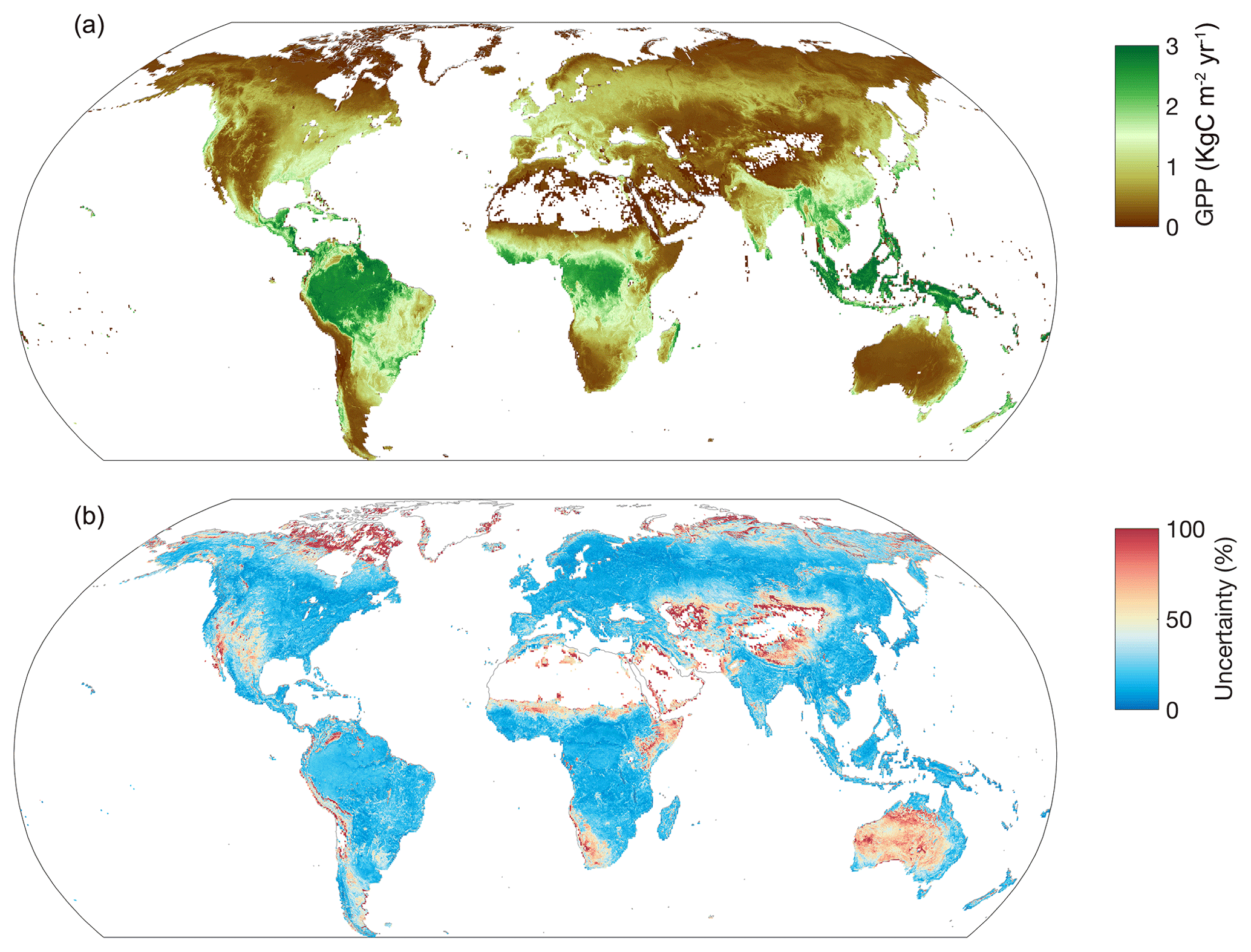
Figure 4Spatial distributions of GPP and its uncertainty. Panel (a) shows the spatial distribution of mean annual GPP, and panel (b) shows the relative uncertainties (calculated as a ratio of interquartile range to mean). The ranges of both the color bars approximately span between the 1st and the 99th percentiles of the data.
4.5 The ecosystem carbon turnover times and associated uncertainties
The ecosystem turnover time and its uncertainty were estimated using different combinations of Csoil, Cveg and GPP data. We calculated τ using full soil depth, which results in a global estimate of 43 yr and ranges from 36 yr (25th percentiles) to 50 yr (75th percentiles). The uncertainty in the global estimate of τ is mainly contributed by soil (84 %) and GPP (15 %), whereas vegetation contributes only marginally (less than 1 %). In addition, we derived a global τ of 37 yr and ranges from 31 to 40 yr by assuming the maximum active layer thickness to be the full soil depth in the circumpolar regions instead of using only 1 m Csoil as was done in the previous study (Carvalhais et al., 2014). The incorporation of deep soil in the circumpolar regions increased the global mean value of τ by 6 yr and uncertainties in the estimations of τ as well. The global spatial distribution of τ (Fig. 5) shows a large heterogeneity which ranges from 7 yr (1st percentile) in the tropics to over 1452 yr (99th percentile) in northern high latitudes. The results show a U-shaped distribution of τ along latitudes in which τ increases by nearly 3 orders of magnitude from low to high latitudes (Fig. 7a). Fig. 5b shows the map of relative uncertainty that is derived from different datasets. The higher relative uncertainty indicates more spread among the datasets used to estimate τ. Our result shows that τ estimates at higher latitudes, especially in circumpolar regions, have higher uncertainties than those at lower latitudes. We found several regions with large spreads in τ among the datasets including northeast Canada, central Russia and central Australia where the relative uncertainties can span beyond 100 %.
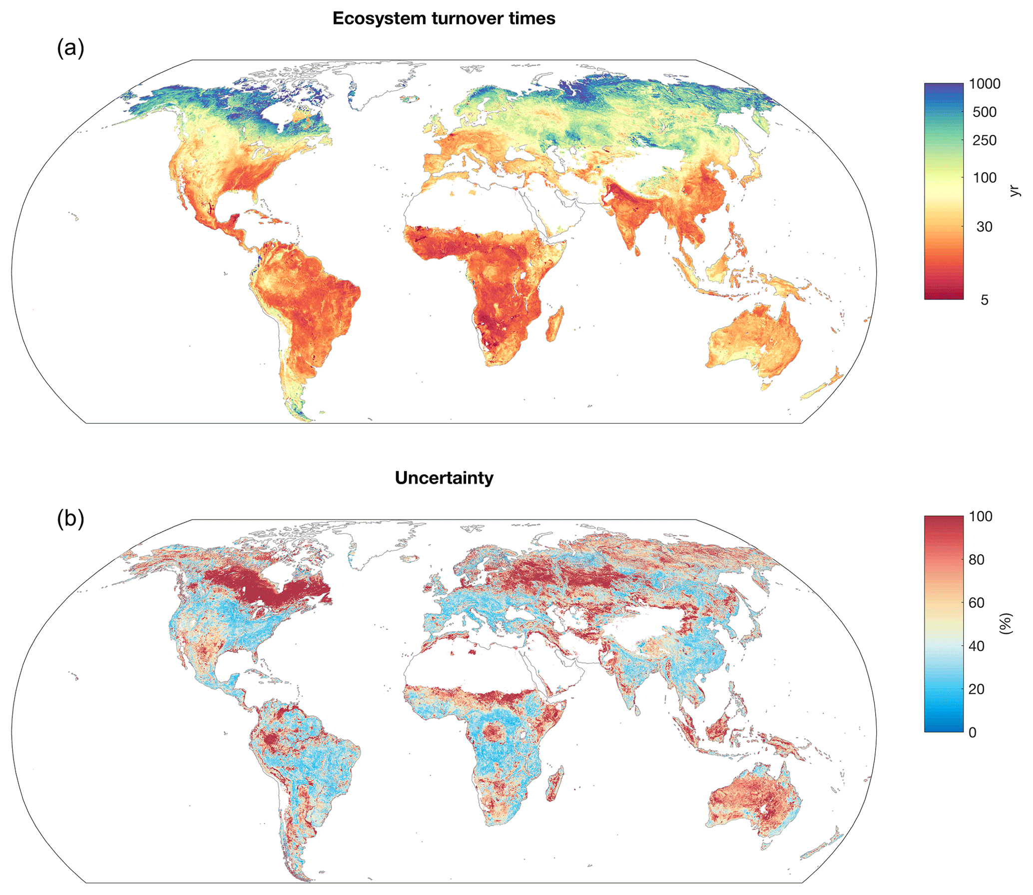
Figure 5Spatial distribution of ecosystem turnover times. Panel (a) shows spatial distribution of turnover times, and panel (b) shows the relative uncertainty (calculated as a ratio of interquartile range / mean). The range of color bar in (a) approximately spans between the 1st and the 99th percentiles of the data, and the one in (b) spans between the 1st and 90th percentiles.
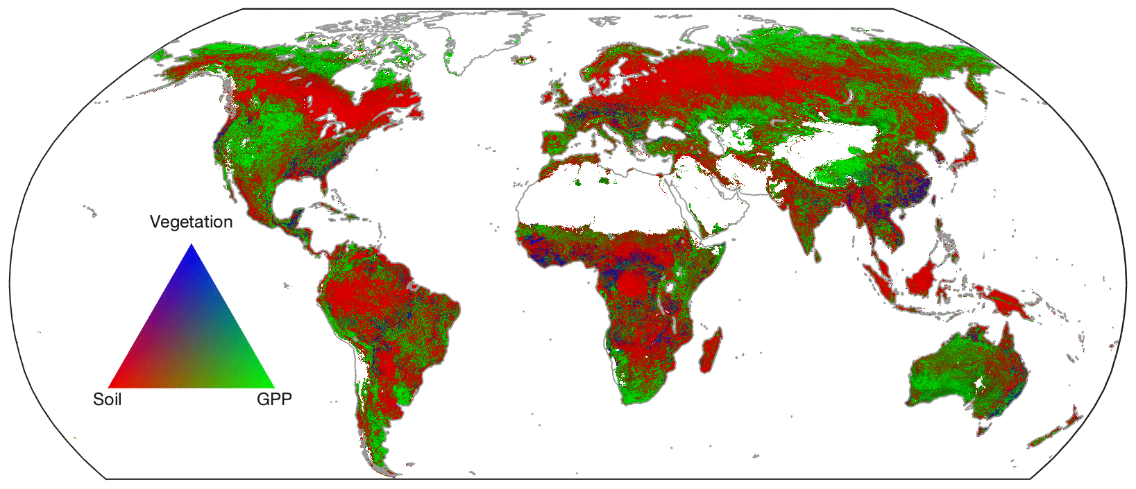
Figure 6The sources of τ uncertainty. The contribution of different sources of soil (at full soil depth), vegetation and GPP data to the uncertainty in turnover time. The green color indicates the regions where the uncertainty is dominated by GPP, red by soil carbon and blue by vegetation carbon. Soil, vegetation and GPP dominate 64.8 %, 32.4 % and 2.7 % of land area in the uncertainty of τ.
4.6 The zonal pattern of turnover times
The latitudinal distributions of τ can be best represented by a second-degree polynomial function (Fig. 7b). After fitting the data of all ensemble members, the rate of τ change with latitude can be obtained by taking the first derivative of the fitted polynomial function. We found that the rate of τ change with latitude has very consistent zonal patterns for different τ ensemble members from different data sources (Fig. 7c). The result shows a consensus in the change in τ with latitude of different datasets. We also found that the zonal τ gradients were not significantly (p>0.05) different from each other for different selections of soil depth, indicating that soil depth has no significant effect on the τ gradient along latitude. It is worth noting that there is a significant difference in the zonal τ gradient between the Northern Hemisphere and Southern Hemisphere (p<0.0001) and that τ increases faster from low to high latitudes in northern latitudes than in the southern latitudes. The results show a high confidence in the zonal distribution of τ and that the difference across datasets does not affect the robustness of the pattern.
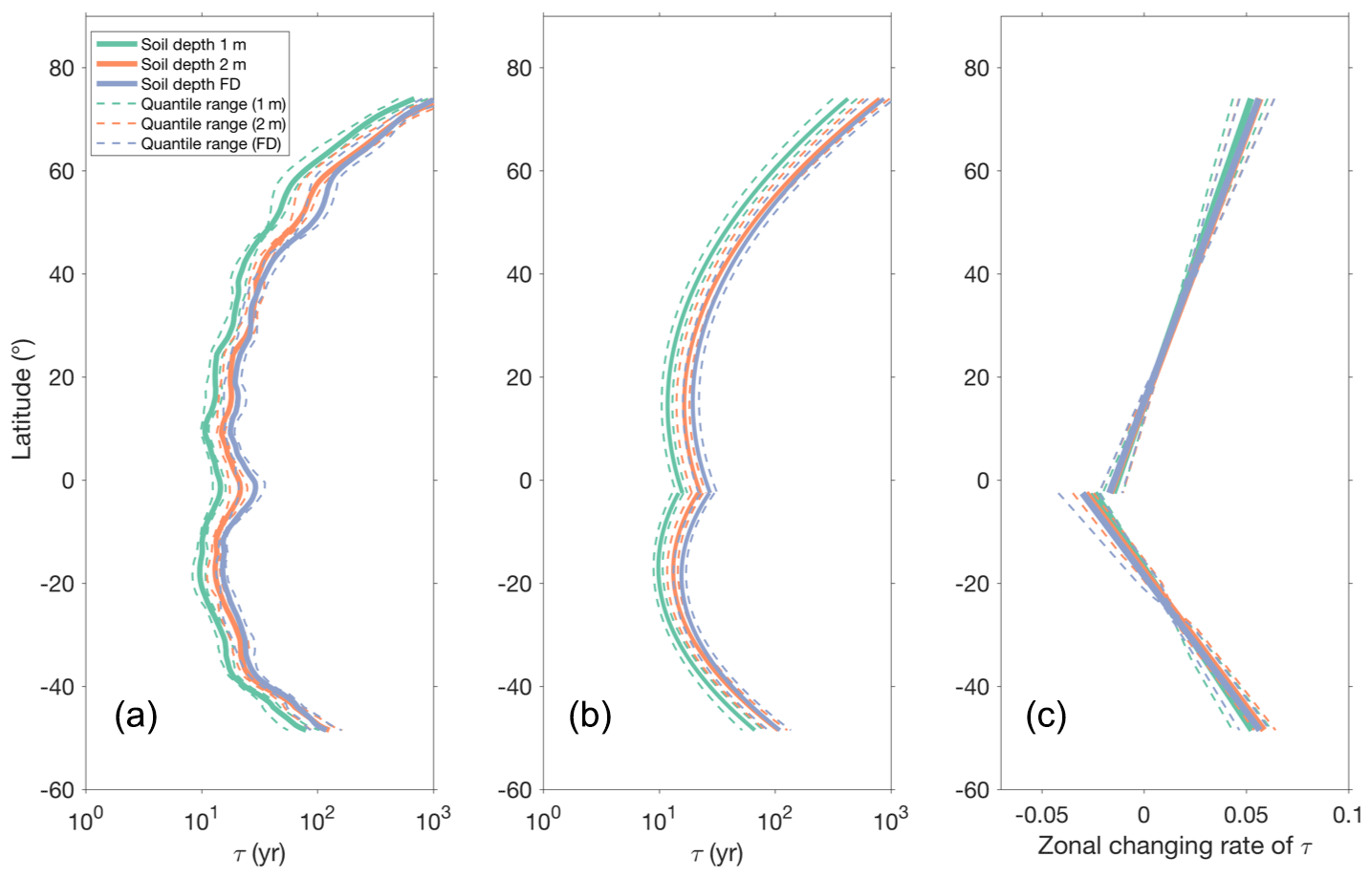
Figure 7(a) The zonal distribution of τ. (b) Second-degree polynomial fit to the zonal distribution of τ. (c) Zonal rate of changes in τ with latitude (calculated as the first derivative of the polynomial function). Solid lines represent the mean τ for different soil depths (1 m, green; 2 m, red; full depth, purple), and dashed lines in the corresponding colors are the interquartile range. The polynomial function is fitted independently for the Northern Hemisphere and Southern Hemisphere. The latitude that divides the Northern Hemisphere and Southern Hemisphere is located at 2∘ S where there is a local maximum of zonal τ in (a).
4.7 The zonal correlation between turnover time and climate
The correlations between τ and temperature and precipitation are analyzed for all the ensemble members on the global scale (see Sect. 3.5). The τ–T correlation (Fig. 8a) is the strongest in northern middle to high latitudes between 25 and 60∘ N, and it decreases rapidly from 20∘ N to the Equator. In the Southern Hemisphere, it increases until 40∘ S, albeit with a weaker gradient than in the Northern Hemisphere. The uncertainties due to differences in the ensemble members (shown by the shaded area) are higher in the transition between the temperate and Arctic regions (50 to 70∘ N), as well as between tropical humid and semiarid regions (20∘ N to 20∘ S). Similar to the contribution of different sources to global uncertainty, the spread in the τ–T correlation is mostly due to Csoil, whereas GPP only affects the zonal correlation to a limited extent (Fig. 8c). However, we find that the τ–T zonal correlation varies negligibly due to data source and soil depth. All ensemble members agree that the τ–T correlation is negative with stronger associations in cold regions than in warm regions.
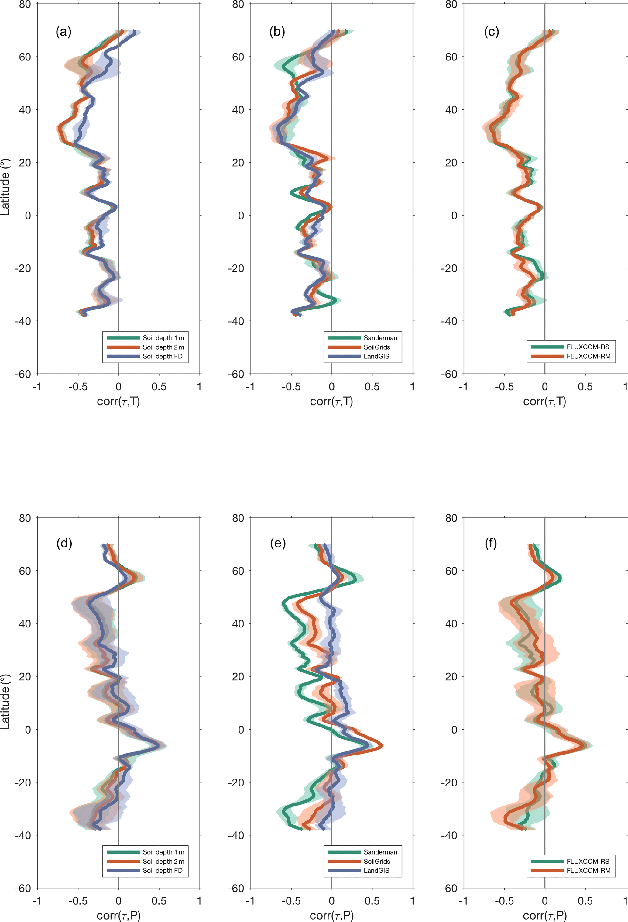
Figure 8Correlation between zonal τ and mean annual temperature (T) and between τ and mean annual precipitation (P). Panels (a) and (d) are colored according to different soil depth (1 m, green; 2 m, red; full soil depth, blue) with shaded areas being the interquartile range. Panels (b) and (e) are colored according to different soil sources. Panels (c) and (f) are colored according to different GPP products of different forcing (remote sensing only and remote sensing plus meteorology). The correlations are consistent across the different latitudinal span widths considered (see Sect. 3.5) and hence are not shown here.
The τ–P correlation, in general, has larger variability across latitude and a higher uncertainty related to differences in Csoil (Fig. 8e). Contrary to the τ–T relationship, the uncertainty of the τ–P correlations from both different data sources and soil depths is smaller in the tropics than at high latitudes. Negative correlations dominate the high latitudes between 20 and 50∘ N and between 20 and 40∘ S. On the other hand, stronger positive correlations prevail in the tropics. The τ–P correlation changes the direction from negative in the temperate zone to positive in the tropics, indicating the role of moisture availability in transitions from arid to humid regions. We also find that the τ–P relationship does not change with different soil depths (Fig. S11 in the Supplement).
The accurate estimation of terrestrial carbon storage and turnover time are essential for understanding carbon cycle–climate feedback (Saatchi et al., 2011; Jobbágy et al., 2000). The present analysis benchmarks carbon storage in soil, vegetation and GPP fluxes from multiple, state-of-the-art, observation-based datasets on a global scale and provides an estimate of the total carbon stock but also estimates of its vertical distribution and spatial variability. In this section, we will discuss the robustness of the current state-of-the-art estimation on global terrestrial carbon turnover times resulting from the different stock and flux components of τ, as well as the robustness of its covariation with climate. We first show the variation of the spatial and vertical distribution of carbon stock in different regions and the possible reason for the difference, and we then discuss the robustness of zonal distribution of turnover times and zonal changing rates across different datasets. Finally, we focus on the sensitivity of turnover times to climate and potential implications.
5.1 Estimation of global soil carbon stocks
We found that there is a significant difference across the current soil carbon datasets in both circumpolar and non-circumpolar regions (Figs. 1 and 2). The results show that the uncertainty of Csoil estimations in the circumpolar regions (52 %) is much larger than that in the non-circumpolar regions (37 %). The spatial patterns of total ecosystem Csoil among the soil datasets are more consistent in the non-circumpolar regions, indicating a higher confidence in the current estimation of soil carbon stock in these regions. In contrast to the non-circumpolar regions, there is lower confidence in the circumpolar regions in estimating Csoil due to the fact that there is a low spatial correlation across datasets (Fig. 1). The difference can be caused by a variety of reasons: for example, (i) as an important input to the machine learning methods, in situ soil profiles are very important factors that influence the final results of the upscaling and, using different training datasets, can lead to relevant differences in outputs, and (ii) the sparse coverage of soil profiles in the circumpolar regions may cause the large divergence in the northern circumpolar region. A major difference in the Sanderman soil dataset compared to the other two soil datasets (SoilGrids and LandGIS) is that here the direct target of upscaling was the soil carbon stock, while in the other two datasets, the targets were each individual component used to calculate Csoil (carbon density, bulk density and percentage of coarse fragments) which were predicted individually. Additional discrepancies may also be associated with the differences in climatic and other input covariates used in the upscaling which may yield a different estimation of Csoil (see Sect. 2.1).
The estimation of a whole ecosystem turnover time is dependent on an estimate of soil carbon stock up to full soil depth. Here, we rely on the available global datasets to follow an ensemble approach for predicting Csoil at full depth that selects models with a minimum distance between prediction and observations by using in situ soil profiles (see Sect. S3 in the Supplement). The final results depend on the information from the global soil datasets and also on the characteristics of the empirical models. Recent studies have shown the advantage of convolutional neural networks, in comparison to random forest approaches (Hengl et al., 2017; Wheeler et al., 2018), for more robust predictions of soil organic carbon (SOC) with depth (Wadoux et al., 2019; Padarian et al., 2019), which could improve the geographical representation of SOC with depth, although random forest approaches already tend to provide unbiased estimates. Overall, the extrapolation provides insights into the carbon storage vertical distribution in deeper soil layers globally, showing that there is approximately 18 % of carbon stored below 2 m globally and over 20 % of carbon stored below 2 m in the circumpolar regions. This results from the fact that, in contrast to the non-circumpolar regions, the circumpolar Csoil does not have a decreasing trend up to 4 m of soil depth (Fig. S1 in the Supplement), which indicates that there is a significant amount of carbon stored in deep soil and emphasizes the perspective that deep soil turnover is a key aspect of the global carbon cycle still poorly understood (Todd-Brown et al., 2013).
5.2 Consistency in vegetation carbon stocks estimations
Compared to soil carbon, the higher level of consistency in the Cveg estimates indicates the stronger agreement on the current estimations in the aboveground carbon components. We show that due to much lower uncertainties in the Cveg estimates, the effect of vegetation on the global τ estimates is minor regardless of which soil depth is used (Table S3). Although the contribution of vegetation to the uncertainties in global τ estimates is less than 2 %, our results show that, locally, vegetation can be the major factor that causes the difference in τ estimates. As shown in Fig. S10 in the Supplement, vegetation dominates the uncertainties of τ in part of the tropics and part of the temperate region in Southeast Asia which in total account for 7 % of the global land area if only 1 m of Csoil is used to estimate τ. The land area where τ uncertainties are dominated by vegetation carbon stocks decreases to 3 % and 1 %, respectively, when Csoil of 2 m and full soil depths is considered. Although our results indicate that vegetation plays a minor role in the global estimates of τ, it is an important factor that can largely affect local patterns of the distribution of τ.
5.3 Differences in global GPP fluxes
The contribution of vegetation and GPP to the uncertainties in global τ is modest compared to the contributions from soil carbon stocks. However, we note that the regional differences in the products can significantly affect the spatial distribution and uncertainty of τ (Figs. 3 and 4). Alternate GPP estimates are likely to impact τ estimates, although marginally. For example, on global scales, the estimate of a GPP of 123 PgC yr−1 by Zhang et al. (2017) would lead to a reduction in τ of ∼10 % compared to our current estimates (43 yr). However, the difference is well within the range of our estimated uncertainty in τ (∼20 %) using all the ensemble members. Given the robustness in spatial patterns in GPP estimate from Zhang et al. (2017) compared to the FLUXCOM estimates (r≥0.9, p<0.01; Fig. S8 in the Supplement), the spatial variability in τ shows a high correlation (r≥0.92, p<0.01) (See Fig. S9 in the Supplement).
5.4 Terrestrial carbon turnover times and associated uncertainties
The current global estimates of τ are substantially larger than previously (60 %), although the global patterns are comparable to previous estimates. Our results show an overall agreement of r=0.95 between the current estimation and the previous estimation of the latitudinal gradient of τ (Carvalhais et al., 2014). The patterns in the latitudinal correlations between climate and τ are also qualitatively similar to the previous patterns found with some particular exceptions in the strength of correlations between τ and temperature in northern temperate systems and changes in τ–precipitation correlations, especially in the tropics. A further investigation on the causes behind these differences between the previous and current studies reflects that Csoil has a substantial contribution to these changes in the correlation between τ and climate, while GPP has only a modest role in altering the τ–temperature correlation changes in northern temperate regions (see Fig. S6 in the Supplement). This is consistent with the assessment of the largest differences in the spatial distribution of Csoil between the three soil datasets used in this study and the HWSD soil dataset used before (Fig. 1).
The uncertainty analysis showed that our current estimation of τ has a considerable spread which is derived from state-of-the-art observations of carbon stocks in soils and vegetation and of carbon fluxes. The uncertainty mainly stems from the soil carbon stocks (84 %) and GPP fluxes (15 %), in which the former dominates the vast areas in the circumpolar regions and the tropical peatland, while the latter dominates the semiarid and arid regions (Fig. 6). Although GPP shows a strong agreement in global spatial patterns, local differences between estimates can lead to significant differences in the estimation of τ. This result is consistent with previous observations and model-based studies that also refer to the biases in estimated primary productivity in affecting the carbon turnover estimations to a large extent (Todd-Brown et al., 2013).
In contrast to global modeling approaches, previous studies have shown that the global soil carbon stocks across observation-based datasets are much less divergent than the ESM simulations included in CMIP5 (Carvalhais et al., 2014). The CMIP5 results show that the simulated carbon storage ranges from 500 to 3000 PgC, implying a 3-fold variation in τ across models (Todd-Brown et al. 2013; Carvalhais et al., 2014). Our current results show that the total amount of carbon in terrestrial ecosystems is substantially higher than the estimation by ESMs, in which even the lowest estimation of total carbon storage (in the Sanderman dataset) is about 300 PgC higher than the highest ESM estimation (MPI-ESM-LR; Todd-Brown et al., 2013). The spatial distribution of carbon stocks among ESMs shows a large variation across models (Carvalhais et al., 2014), while the observation-based datasets are more consistent in the non-circumpolar regions. However, the uncertainty analysis shows that our current estimation of τ has a considerable spread resulting mainly from the spread in state-of-the-art estimates of soil carbon stocks, followed by the spread in estimates of GPP. The estimation of τ is dependent on the assumption of a maximum soil depth used to estimate soil C stocks that particularly in the circumpolar regions contribute 54 % to the overall uncertainty, while the data source contributes 25 %. Soil depth itself is characterized by a large uncertainty given the difficulty in assessing in situ measurement uncertainties in defining a depth at which the soil becomes metabolically inactive and in determining the role of vertical transport to a depth-dependent concentration. The challenge in circumpolar regions relates additionally to the influence of active layer dynamics on the spatial and temporal variability in metabolic activity. From an ESM perspective, it is difficult to avoid relying on a whole soil, or ecosystem, estimate to compare it with observation-based estimates given that these models abstract from depth-dependent soil carbon decomposition dynamics or have not reported the depth of the soil carbon stocks (Carvalhais et al., 2014). In this aspect, an explicit consideration of soil C stocks at depth in ESMs would be instrumental in understanding and evaluating the distribution of ecosystem carbon stocks and turnover times against observations.
It is worth noting that here the estimation of τ is based on the steady-state assumption, which is the assumption of a balanced net exchange of carbon between terrestrial ecosystems and the atmosphere. Here, the assumption is that integrating at larger spatial scales, by averaging the local variations in sink and source conditions, reduces the differences between assimilation and outflux relative to the gross influx and that the integration of stocks and fluxes for long-term spans reduces the effects of transient changes in climate and of interannual variability in τ estimates. However, this assumption is valid to a significantly lesser extent at smaller spatial scales (site-level) and shorter time intervals since the ecosystem–atmosphere exchange of carbon is most of the time not in balance, and forced steady-state assumptions can lead to biases in estimates of turnover times and other ecosystem parameters (Ge et al., 2018; Carvalhais et al., 2008).
5.5 Robust associations of τ and climate
Despite the large uncertainty in the τ estimations, we identified robust patterns in the τ–climate relationship that can be instrumental in addressing the large uncertainties in modeling the sensitivity of terrestrial carbon to climate, which are reflected in the spread of τ estimates by the different ESMs (Tod-Brown et al., 2013). The zonal distribution of τ is a robust feature that changes little across different datasets, which indicates that the current state-of-the-art datasets all agree on the latitudinal gradient of the carbon turnover time (Fig. 7). In addition, the latitudinal change rate of τ is robust against any considered soil depth (Fig. 7), which reflects pattern comparability between assumptions of τ gradients up to 1 m (Koven et al. 2017; Wang et al., 2018) or to full soil depth (Carvalhais et al., 2014). The robustness of the latitudinal patterns in the ensemble is likely to emerge from the latitudinal gradient in temperature, shaping the zonal distribution of τ that increases towards the poles as mean annual temperatures substantially decrease.
This study addresses the robustness of the τ–climate association by investigating the zonal correlations between τ and temperature and between τ and precipitation. The τ–temperature correlation varies with latitude in which high correlations are found at higher latitudes and low to moderate correlations are found closer to the tropics (Fig. 8). The latitudinal gradient in the τ–T relationship is similar when compared with previous results (Carvalhais et al., 2014), although the strength of the correlations can vary marginally by changing GPP products but more substantially when exchanging the Csoil datasets (Fig. S6 in the Supplement). However, these relationships show strong robustness across state-of-the-art datasets (Fig. 8). On the other hand, the zonal patterns of τ–precipitation are more challenging to converge across different Csoil sources (Fig. 8e) when compared with uncertainties stemming from GPP (Fig. 8f) regardless of the depth considered (Fig. S11 in the Supplement). Overall, the correlation between turnover times and precipitation in the tropics is higher than that with temperature, as shown in Fig. 8d, indicating a potentially more dominant role of precipitation in the tropics (Wang et al., 2018).
Overall, the τ–P correlations, although varying in strength, are robust across the data ensemble except when controlling for Csoil source (Fig. 8e). The role of Csoil in the τ–P relationships is independent of depth (Fig. S11 in the Supplement) and explains most of the differences found in the patterns of previous results (Carvalhais et al., 2014), which are mainly caused by the differences in the soil carbon stock (Fig. S6 in the Supplement). Given that the data and methodological support are substantially shared across the different approaches (see Sect. 2.1) and given the potential limitations in representing contributions of soil moisture to τ at deeper layers, even shallower than 2 m, these results highlight the relevance of better understanding and diagnosing the effects of the hydrological cycle on τ. The limitation may be linked to the realization that methods based on random forests tend to show high correlations between predicted top soil and deeper soil estimates of Csoil, as well as lower correlations to deeper Csoil geographic variability (Wadoux et al., 2019; Padarian et al., 2019).
Ultimately, given the recognition that the sensitivity of the terrestrial carbon to climate is a major uncertainty reflected in the spread of τ across different ESMs, the reliable estimation of τ and identification of robust patterns in τ–climate associations is key to provide robust constraints to improve the performance of the current ESMs. Notwithstanding, the intimate interaction of energy and water along with other factors such as land use change all affect τ but on different spatial and temporal scales. Further research directions would gain by exploring the contribution of addition potential factors that may influence the spatial distribution of τ, such as mortality and disturbance regimes, human impact via management regimes or land cover change dynamics, and the vertical distribution of the hydrological cycles.
The dataset of the entire ecosystem turnover times of carbon presented in this study can be downloaded from the Data Portal of the Max Planck Institute for Biogeochemistry at https://doi.org/10.17871/bgitau.201911 (Fan et al., 2019).
A full assessment of the global turnover times of carbon is provided using an observation-based ensemble of current state-of-the-art datasets of soil carbon stocks, vegetation biomass and GPP. On the global scale, the uncertainties in τ estimates are dominated by the large uncertainties in soil carbon stocks. The uncertainty of carbon stocks and τ estimation in the circumpolar regions is significantly higher than that in the non-circumpolar regions. Our results show that there is a consistent vertical distribution of soil carbon across datasets, and it is estimated that soils below 2 m comprise up to 20 % of total soil carbon globally. A spatial analysis shows that both soil carbon and GPP are the major contributors to local uncertainties in τ estimation. The differences in soil stocks between datasets dominate the uncertainties of τ in the circumpolar regions, while the spread in GPP dominates the uncertainty in semiarid and arid regions. The difference in vegetation data has a minor contribution to the uncertainty.
Despite the differences, we identified several robust patterns that change only marginally across different ensemble members of τ that derived from different datasets or different soil depths. First, we found a consistent latitudinal pattern in τ that can be described by a second-degree polynomial function. The changing rate of τ with latitude can be described equally well for all ensemble members, and the changing rate of τ with latitude is highly consistent across different datasets and does not change with soil depth. The same zonal correlations between τ and climate showed there is a robust association of τ with temperature and with precipitation. However, we note that the association between temperature and precipitation and τ change with latitude. Specifically, temperature mainly affects the τ variation in middle to high latitudes beyond 20∘ N and 20∘ S, while precipitation affects τ not only in temperate zones but also in the tropical regions. Overall, this study synthesizes the current state-of-the-art data on global carbon turnover estimation and argues that the zonal distribution of τ and its covariation with climate is robust across the diverse observation-based ensemble considered here. These results build on previous efforts and support exercises for benchmarking ESMs.
The supplement related to this article is available online at: https://doi.org/10.5194/essd-12-2517-2020-supplement.
NF and NC designed the study. NF conducted analysis and wrote the paper under the direction of NC. MT, VA and MS provided data for the analysis. NF and UW collected and harmonized datasets. NF, UW and SK contributed to methodological development. SK participated in the discussion and development of the paper. All authors contributed to the discussions and interpretation of the results and the writing of the paper.
The authors declare that they have no conflict of interest.
We would like to acknowledge the support of Tomislav Hengl for providing soil carbon data and discussions regarding the analysis. We would like to thank Saatchi Sassan for providing one of the vegetation biomass datasets. We thank Martin Jung for providing GPP data and useful feedback and Jacob A. Nelson for suggestions on improving the paper's language.
This research has been supported by the International Max Planck Research School for Global Biogeochemical Cycle and the European Space Agency (grant no. No. 4000113100/14/I-NB).
This paper was edited by David Carlson and reviewed by two anonymous referees.
Avitabile, V., Herold, M., Heuvelink, G., Lewis, S. L., Phillips, O. L., Asner, G. P., Armston, J., Ashton, P. S., Banin, L., and Bayol, N.: An integrated pan-tropical biomass map using multiple reference datasets, Glob. Change Biol., 22, 1406–1420, https://doi.org/10.1111/gcb.13139, 2016.
Baccini, A., Goetz, S., Walker, W., Laporte, N., Sun, M., Sulla-Menashe, D., Hackler, J., Beck, P., Dubayah, R., and Friedl, M.: Estimated carbon dioxide emissions from tropical deforestation improved by carbon-density maps, Nat. Clim. Change, 2, 182–185, 2012.
Barrett, D. J.: Steady state turnover time of carbon in the Australian terrestrial biosphere, Global Biogeochem. Cy., 16, 55-1–55-21, 2002.
Batjes, N.: Harmonized soil property values for broad-scale modelling (WISE30sec) with estimates of global soil carbon stocks, Geoderma, 269, 61–68, 2016.
Batjes, N. H., Ribeiro, E., and van Oostrum, A.: Standardised soil profile data to support global mapping and modelling (WoSIS snapshot 2019), Earth Syst. Sci. Data, 12, 299–320, https://doi.org/10.5194/essd-12-299-2020, 2020.
Bolin, B. and Rodhe, H.: A note on the concepts of age distribution and transit time in natural reservoirs, Tellus, 25, 58–62, 1973.
Carvalhais, N., Reichstein, M., Seixas, J., Collatz, G. J., Pereira, J. S., Berbigier, P., Carrara, A., Granier, A., Montagnani, L., and Papale, D.: Implications of the carbon cycle steady state assumption for biogeochemical modeling performance and inverse parameter retrieval, Global Biogeochem. Cy., 22, GB2007, https://doi.org/10.1029/2007GB003033, 2008.
Carvalhais, N., Forkel, M., Khomik, M., Bellarby, J., Jung, M., Migliavacca, M., Mu, M., Saatchi, S., Santoro, M., Thurner, M., Weber, U., Ahrens, B., Beer, C., Cescatti, A., Randerson, J. T., and Reichstein, M.: Global covariation of carbon turnover times with climate in terrestrial ecosystems, Nature, 514, 213–217, 2014.
Davidson, E. A. and Janssens, I. A.: Temperature sensitivity of soil carbon decomposition and feedbacks to climate change, Nature, 440, 165–173, 2006.
Fan, N., Koirala, S., Reichstein, M., Thurner, M., Avitabile, V., Santoro, M., Ahrens, B., Weber, U., and Carvarhais, N.: Ecosystem turnover time database, MPI-BGC, https://doi.org/10.17871/bgitau.201911, 2019.
Fick, S. E. and Hijmans, R. J.: WorldClim 2: new 1-km spatial resolution climate surfaces for global land areas, Int. J. Climatol., 37, 4302-4315, https://doi.org/10.1002/joc.5086, 2017.
Friedlingstein, P., Cox, P., Betts, R., Bopp, L., Von Bloh, W., Brovkin, V., Cadule, P., Doney, S., Eby, M., and Fung, I.: Climate–carbon cycle feedback analysis: results from the C4MIP model intercomparison, J. Climate, 19, 3337–3353, 2006.
Friend, A. D., Lucht, W., Rademacher, T. T., Keribin, R., Betts, R., Cadule, P., Ciais, P., Clark, D. B., Dankers, R., and Falloon, P. D.: Carbon residence time dominates uncertainty in terrestrial vegetation responses to future climate and atmospheric CO2, P. Natl. Acad. Sci. USA, 111, 3280–3285, 2014.
Ge, R., He, H., Ren, X., Zhang, L., Yu, G., Smallman, T. L., Zhou, T., Yu, S. Y., Luo, Y., and Xie, Z.: Underestimated ecosystem carbon turnover time and sequestration under the steady state assumption: a perspective from long-term data assimilation, Glob. Change Biol., 25, 938-953, https://doi.org/10.1111/gcb.14547, 2018.
Generation 3 Database Reports: Nave, L., Johnson, K., van Ingen, C., Agarwal, D., Humphrey, M., and Beekwilder, N: International Soil Carbon Network (ISCN) Database, Version 3, Database Report: ISCN_SOC-DATA_LAYER_1-1, https://doi.org/10.17040/ISCN/1305039, 2017.
Hansen, N. and Ostermeier, A.: Completely Derandomized Self-Adaptation in Evolution Strategies, Evol. Comput., 9, 159–195, https://doi.org/10.1162/106365601750190398, 2001.
Hengl, T., de Jesus, J. M., MacMillan, R. A., Batjes, N. H., Heuvelink, G. B., Ribeiro, E., Samuel-Rosa, A., Kempen, B., Leenaars, J. G., and Walsh, M. G.: SoilGrids1km – global soil information based on automated mapping, PloS one, 9, e105992, https://doi.org/10.1371/journal.pone.0105992, 2014.
Hengl, T., de Jesus, J. M., Heuvelink, G. B., Gonzalez, M. R., Kilibarda, M., Blagotić, A., Shangguan, W., Wright, M. N., Geng, X., and Bauer-Marschallinger, B.: SoilGrids250m: Global gridded soil information based on machine learning, PloS one, 12, e0169748, https://doi.org/10.1371/journal.pone.0169748, 2017.
Hugelius, G., Bockheim, J. G., Camill, P., Elberling, B., Grosse, G., Harden, J. W., Johnson, K., Jorgenson, T., Koven, C. D., Kuhry, P., Michaelson, G., Mishra, U., Palmtag, J., Ping, C.-L., O'Donnell, J., Schirrmeister, L., Schuur, E. A. G., Sheng, Y., Smith, L. C., Strauss, J., and Yu, Z.: A new data set for estimating organic carbon storage to 3 m depth in soils of the northern circumpolar permafrost region, Earth Syst. Sci. Data, 5, 393–402, https://doi.org/10.5194/essd-5-393-2013, 2013.
Jackson, R. B., Lajtha, K., Crow, S. E., Hugelius, G., Kramer, M. G., and Piñeiro, G.: The ecology of soil carbon: pools, vulnerabilities, and biotic and abiotic controls, Annu. Rev. Ecol. Evol. Syst., 48, 419–445, https://doi.org/10.1146/annurev-ecolsys-112414-054234, 2017.
Jobbágy, E. G. and Jackson, R. B.: The vertical distribution of soil organic carbon and its relation to climate and vegetation, Ecol. Appl., 10, 423–436, 2000.
Jung, M., Henkel, K., Herold, M., and Churkina, G.: Exploiting synergies of global land cover products for carbon cycle modeling, Remote Sens. Environ., 101, 534–553, 2006.
Jung, M., Reichstein, M., Schwalm, C. R., Huntingford, C., Sitch, S., Ahlström, A., Arneth, A., Camps-Valls, G., Ciais, P., and Friedlingstein, P.: Compensatory water effects link yearly global land CO2 sink changes to temperature, Nature, 541, 516–520, 2017.
Jung, M., Schwalm, C., Migliavacca, M., Walther, S., Camps-Valls, G., Koirala, S., Anthoni, P., Besnard, S., Bodesheim, P., Carvalhais, N., Chevallier, F., Gans, F., Goll, D. S., Haverd, V., Köhler, P., Ichii, K., Jain, A. K., Liu, J., Lombardozzi, D., Nabel, J. E. M. S., Nelson, J. A., O'Sullivan, M., Pallandt, M., Papale, D., Peters, W., Pongratz, J., Rödenbeck, C., Sitch, S., Tramontana, G., Walker, A., Weber, U., and Reichstein, M.: Scaling carbon fluxes from eddy covariance sites to globe: synthesis and evaluation of the FLUXCOM approach, Biogeosciences, 17, 1343–1365, https://doi.org/10.5194/bg-17-1343-2020, 2020.
Koven, C. D., Hugelius, G., Lawrence, D. M., and Wieder, W. R.: Higher climatological temperature sensitivity of soil carbon in cold than warm climates, Nat. Clim. Change, 7, 817–822, https://doi.org/10.1038/nclimate3421, 2017.
Padarian, J., Minasny, B., and McBratney, A. B.: Using deep learning for digital soil mapping, SOIL, 5, 79–89, https://doi.org/10.5194/soil-5-79-2019, 2019.
Raich, J. and Schlesinger, W. H.: The global carbon dioxide flux in soil respiration and its relationship to vegetation and climate, Tellus B, 44, 81–99, https://doi.org/10.3402/tellusb.v44i2.15428, 1992.
Saatchi, S. S., Harris, N. L., Brown, S., Lefsky, M., Mitchard, E. T., Salas, W., Zutta, B. R., Buermann, W., Lewis, S. L., and Hagen, S.: Benchmark map of forest carbon stocks in tropical regions across three continents, P. Natl. Acad. Sci. USA, 108, 9899–9904, 2011.
Sanderman, J., Hengl, T., and Fiske, G. J.: Soil carbon debt of 12,000 years of human land use, P. Natl. Acad. Sci. USA, 114, 9575–9580, 2017.
Santoro, M., Beaudoin, A., Beer, C., Cartus, O., Fransson, J. E., Hall, R. J., Pathe, C., Schmullius, C., Schepaschenko, D., and Shvidenko, A.: Forest growing stock volume of the northern hemisphere: Spatially explicit estimates for 2010 derived from Envisat ASAR, Remote Sens. Environ., 168, 316–334, 2015.
Santoro, M., Cartus, O., Mermoz, S., Bouvet, A., Le Toan, T., Carvalhais, N., Rozendaal, D., Herold, M., Avitabile, V., Quegan, S., Carreiras, J., Rauste, Y., Balzter, H., Schmullius, C., Seifert, F. M.: A detailed portrait of the forest aboveground biomass pool for the year 2010 obtained from multiple remote sensing observations, 20th EGU General Assembly, EGU2018, Proceedings from the conference held 4–13 April 2018 in Vienna, Austria, p. 18932, available at: https://ui.adsabs.harvard.edu/abs/2018EGUGA..2018932S/abstract (last access: 5 August 2019), 2018.
Santoro, M., Cartus, O., Carvalhais, N., Rozendaal, D., Avitabilie, V., Araza, A., de Bruin, S., Herold, M., Quegan, S., Rodríguez Veiga, P., Balzter, H., Carreiras, J., Schepaschenko, D., Korets, M., Shimada, M., Itoh, T., Moreno Martínez, Á., Cavlovic, J., Cazzolla Gatti, R., da Conceição Bispo, P., Dewnath, N., Labrière, N., Liang, J., Lindsell, J., Mitchard, E. T. A., Morel, A., Pacheco Pascagaza, A. M., Ryan, C. M., Slik, F., Vaglio Laurin, G., Verbeeck, H., Wijaya, A., and Willcock, S.: The global forest above-ground biomass pool for 2010 estimated from high-resolution satellite observations, Earth Syst. Sci. Data Discuss., https://doi.org/10.5194/essd-2020-148, in review, 2020.
Thurner, M., Beer, C., Santoro, M., Carvalhais, N., Wutzler, T., Schepaschenko, D., Shvidenko, A., Kompter, E., Ahrens, B., and Levick, S. R.: Carbon stock and density of northern boreal and temperate forests, Global Ecol. Biogeogr., 23, 297–310, https://doi.org/10.1111/geb.12125, 2014.
Thurner, M., Beer, C., Ciais, P., Friend, A. D., Ito, A., Kleidon, A., Lomas, M. R., Quegan, S., Rademacher, T. T., and Schaphoff, S.: Evaluation of climate‐related carbon turnover processes in global vegetation models for boreal and temperate forests, Global Change Biol., 23, 3076–3091, https://doi.org/10.1111/gcb.13660, 2017.
Tifafi, M., Guenet, B., and Hatté, C.: Large differences in global and regional total soil carbon stock estimates based on SoilGrids, HWSD, and NCSCD: Intercomparison and evaluation based on field data from USA, England, Wales, and France, Global Biogeochem. Cy., 32, 42–56, https://doi.org/10.1002/2017GB005678, 2018.
Todd-Brown, K. E. O., Randerson, J. T., Post, W. M., Hoffman, F. M., Tarnocai, C., Schuur, E. A. G., and Allison, S. D.: Causes of variation in soil carbon simulations from CMIP5 Earth system models and comparison with observations, Biogeosciences, 10, 1717–1736, https://doi.org/10.5194/bg-10-1717-2013, 2013.
Todd-Brown, K. E. O., Randerson, J. T., Hopkins, F., Arora, V., Hajima, T., Jones, C., Shevliakova, E., Tjiputra, J., Volodin, E., Wu, T., Zhang, Q., and Allison, S. D.: Changes in soil organic carbon storage predicted by Earth system models during the 21st century, Biogeosciences, 11, 2341–2356, https://doi.org/10.5194/bg-11-2341-2014, 2014.
Tramontana, G., Jung, M., Schwalm, C. R., Ichii, K., Camps-Valls, G., Ráduly, B., Reichstein, M., Arain, M. A., Cescatti, A., Kiely, G., Merbold, L., Serrano-Ortiz, P., Sickert, S., Wolf, S., and Papale, D.: Predicting carbon dioxide and energy fluxes across global FLUXNET sites with regression algorithms, Biogeosciences, 13, 4291–4313, https://doi.org/10.5194/bg-13-4291-2016, 2016.
Wadoux, A. M. J.-C., Padarian, J., and Minasny, B.: Multi-source data integration for soil mapping using deep learning, SOIL, 5, 107–119, https://doi.org/10.5194/soil-5-107-2019, 2019.
Wang, J., Sun, J., Xia, J., He, N., Li, M., and Niu, S.: Soil and vegetation carbon turnover times from tropical to boreal forests, Funct. Ecol., 32, 71–82, https://doi.org/10.1111/1365-2435.12914, 2018.
Webb, R., Rosenzweig, C. E., and Levine, E. R.: Global Soil Texture and Derived Water-Holding Capacities, ORNL DAAC, Oak Ridge, TN, USA, https://doi.org/10.3334/ORNLDAAC/548, 2000.
Wenzel, S., Cox, P. M., Eyring, V., and Friedlingstein, P.: Emergent constraints on climate-carbon cycle feedbacks in the CMIP5 Earth system models, J. Geophys. Res.-Biogeo., 119, 794–807, https://doi.org/10.1002/2013JG002591, 2014.
Wheeler, I., Hengl, T.: Soil organic carbon stock in kg∕m2 time-series 2001–2015 based on the land cover changes (Version v0.2) [Data set], Zenodo, https://doi.org/10.5281/zenodo.2529721, 2018.
Zhang, Y., Xiao, X., Wu, X., Zhou, S., Zhang, G., Qin, Y., and Dong, J.: A global moderate resolution dataset of gross primary production of vegetation for 2000–2016, Sci. Data, 4, 170165, https://doi.org/10.1038/sdata.2017.165, 2017.