Glacier shrinkage in the Alps continues unabated as revealed by a new glacier inventory from Sentinel-2

The ongoing glacier shrinkage in the Alps requires frequent updates of glacier outlines to provide an accurate database for monitoring, modelling purposes (e.g. determination of run-off, mass balance, or future glacier extent), and other applications. With the launch of the first Sentinel-2 (S2) satellite in 2015, it became possible to create a consistent, Alpine-wide glacier inventory with an unprecedented spatial resolution of 10 m. The first S2 images from August 2015 already provided excellent mapping conditions for most glacierized regions in the Alps and were used as a base for the compilation of a new Alpine-wide glacier inventory in a collaborative team effort. In all countries, glacier outlines from the latest national inventories have been used as a guide to compile an update consistent with the respective previous interpretation. The automated mapping of clean glacier ice was straightforward using the band ratio method, but the numerous debris-covered glaciers required intense manual editing. Cloud cover over many glaciers in Italy required also including S2 scenes from 2016. The outline uncertainty was determined with digitizing of 14 glaciers several times by all participants. Topographic information for all glaciers was obtained from the ALOS AW3D30 digital elevation model (DEM). Overall, we derived a total glacier area of 1806±60 km² when considering 4395 glaciers >0.01 km². This is 14 % (−1.2 % a⁻¹) less than the 2100 km² derived from Landsat in 2003 and indicates an unabated continuation of glacier shrinkage in the Alps since the mid-1980s. It is a lower-bound estimate, as due to the higher spatial resolution of S2 many small glaciers were additionally mapped or increased in size compared to 2003. Median elevations peak around 3000 m a.s.l., with a high variability that depends on location and aspect. The uncertainty assessment revealed locally strong differences in interpretation of debris-covered glaciers, resulting in limitations for change assessment when using glacier extents digitized by different analysts. The inventory is available at https://doi.org/10.1594/PANGAEA.909133 (Paul et al., 2019).

1 Introduction

Information on glacier extents is required for numerous glaciological and hydrological calculations, ranging from the determination of glacier volume, surface mass balance, and future glacier evolution to run-off, hydropower production, and sea level rise (e.g. Marzeion et al., 2017). For these and several other applications, glacier outlines spatially constrain all calculations and thus provide an important baseline dataset. In response to the ongoing atmospheric warming, glaciers retreat, shrink, and lose mass in most regions of the world (e.g. Gardner et al., 2013; Wouters et al., 2019; Zemp et al., 2019). Accordingly, a frequent update of glacier inventories is required to reduce uncertainties in subsequent calculations. With relative area loss rates of about 1 % a⁻¹ in many regions globally (Vaughan et al., 2013), glaciers lose about 10 % of their area within a decade, and thus a decadal update frequency seems sensible. In regions with stronger glacier shrinkage, such as the tropical Andes (e.g. Rabatel et al., 2013, 2018) or the European Alps (e.g. Gardent et al., 2014), an even higher update frequency is likely required. However, apart from the high workload required to digitize or manually correct glacier outlines (e.g. Racoviteanu et al., 2009), it is often not possible to obtain satellite images in a desired period of the year with appropriate mapping conditions, i.e. without seasonal snow and clouds hiding glaciers. Hence, glacier inventories are often compiled from images acquired over several years, resulting in a temporarily inhomogeneous dataset. Fortunately, a 3-year period of acquisition is still acceptable in error terms, as area changes of about ±3 % are within the typical area uncertainty of about 3 % to 5 % (e.g. Paul et al., 2013).

The last glacier inventory covering the entire Alps with a common and homogeneous date was compiled from Landsat Thematic Mapper (TM) images acquired within 6 weeks in the summer of 2003 (Paul et al., 2011). Although this dataset has its caveats (e.g. missing small glaciers in Italy and some debris-covered ice), it is methodologically and temporarily consistent and represents glacier outlines of the Alps in the Randolph Glacier Inventory (RGI). A few years later, high-quality glacier inventories were compiled from better resolved datasets (aerial photography, airborne laser scanning) on a national level in all four countries of the Alps with substantial glacier coverage (Austria, France, Italy, Switzerland). These more recent inventories refer to the periods 2008–2011 for Switzerland (Fischer et al., 2014), 2004–2011 for Austria (Fischer et al., 2015), 2006–2009 for France (Gardent et al., 2014), and 2005-2011 for Italy (Smiraglia et al., 2015). As an 8-year period is rather long, consistent and comparable change assessment is challenging. However, for the first version of the World Glacier Inventory (WGI) the temporal spread was even larger, ranging from 1959 to about 1983 (Zemp et al., 2008). Another problem for change assessment is the inhomogeneous interpretation of glacier extents that occurs in part to be compliant with the interpretation in earlier national inventories. Hence, calculations over the entire Alps that require a consistent time stamp are difficult to perform and rates of glacier change are difficult to compare across regions (e.g. Gardent et al., 2014).

Considering the ongoing strong glacier shrinkage in the Alps over the past decades and the above shortcomings of existing datasets, there is a high demand to compile a (1) new, (2) precise, and (3) consistent glacier inventory for the entire Alps, with data acquired under (4) good mapping conditions in (5) a single year. Although it might be difficult to satisfy all five criteria at the same time, at least some of them seem achievable by means of recently available satellite data. With the 10 m resolution data from Sentinel-2 (S2) and its 290 km swath width, it is possible (a) to improve the quality of the derived glacier outlines (compared to Landsat TM) substantially (Paul et al., 2016) and (b) cover a region such as the Alps with a few scenes acquired within a few weeks or even days, satisfying criteria (2) and (5). Good mapping conditions, however, only occur by chance after a comparably warm summer when all seasonal snow off glaciers has melted and largely cloud-free conditions persist over an extended time span in August or September.

Here we present a new glacier inventory for the European Alps that has been compiled from S2 data that were mostly acquired within 2 weeks of August 2015 (during the commissioning phase). However, due to glaciers (mostly in Italy) being partly cloud-covered, scenes from 2016 (and very few from 2017) were also used. Hence, criterion (5) could not be fully satisfied. In order to satisfy point (3), we decided to perform the mapping of clean ice with an identical method (band ratio), and distribute the raw outlines to the national experts for editing of wrongly classified regions (e.g. adding missing ice in shadow and under local clouds or debris cover, removing lakes and other water surfaces). As a guide for the interpretation the analysts used the latest high-resolution inventory in each country. All corrected datasets were merged into one dataset and topographic information for each glacier was derived from the ALOS AW3D30 digital elevation model (DEM). For uncertainty assessment all five participants corrected the extents of 14 glaciers independently four times.

2 Study region

The Alps are a largely west–east (south–north in the western part) oriented mountain range in the centre of Europe (roughly from 43 to 49^∘ N and 2 to 18^∘ E) with peaks reaching 4808 m a.s.l. in the west at Mont Blanc (Monte Bianco) and elevations above 3000 m a.s.l. in most regions. In Fig. 1 we show the region covered by glaciers, along with footprints of the Sentinel-2 tiles used for data processing. The Alps thus act as a topographic barrier for air masses coming from the north and south (Auer et al., 2007), as well as from the west in the western part. This results in enhanced orographic precipitation and a high regional variability of precipitation amounts in specific years and in the long-term mean (e.g. Frei et al., 2003). On the other hand, temperatures are horizontally rather uniform (e.g. Böhm et al., 2001) but vary strongly with height according to the atmospheric lapse rate (e.g. Frei, 2014). Snow accumulation is mostly due to winter precipitation, but some snowfall can also occur in summer at higher elevations, reducing ablation for a few days.

Table 1 Details about the Sentinel-2 tiles used to create the inventory; C stands for country. The related Fig. 1 shows where the tiles are located.

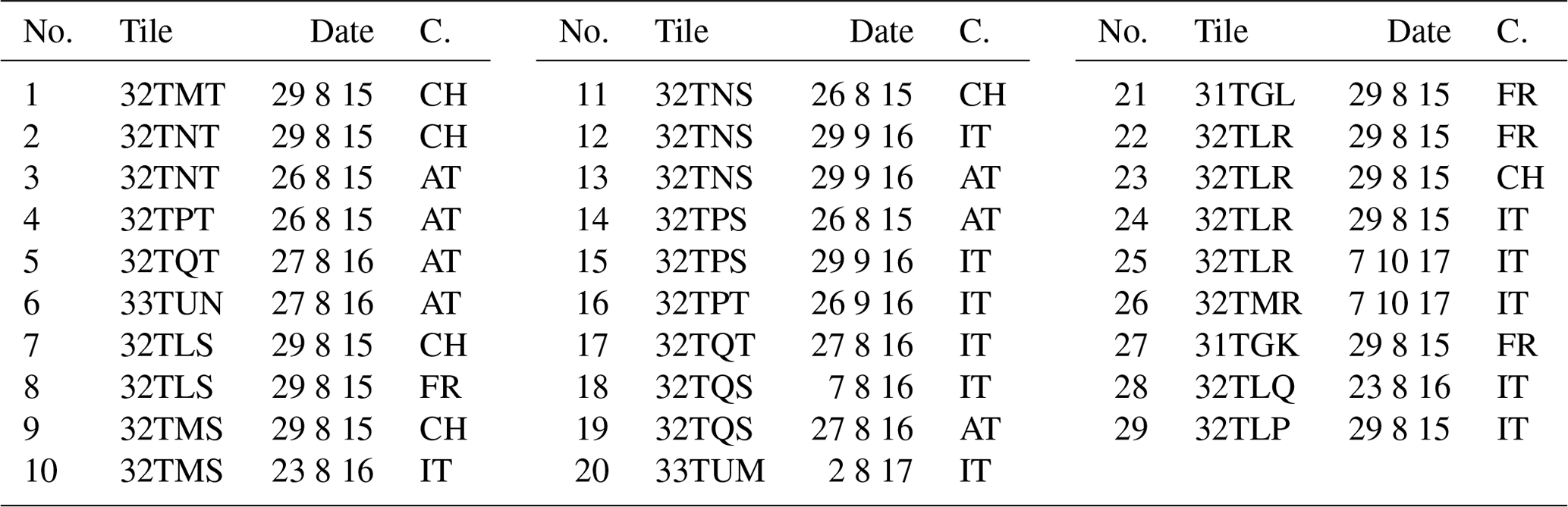
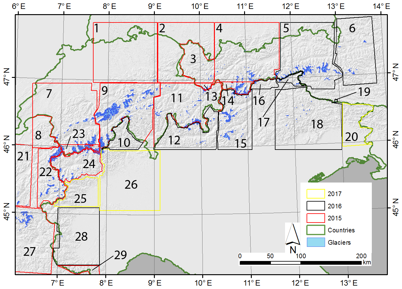
Figure 1 Overview of the study region with footprints (colour-coded for acquisition year) of the Sentinel-2 tiles used (see Table 1 for numbers).

There is no significant long-term trend in precipitation over the last 100+ years (Casty et al., 2005), but summer temperatures in the Alps increased sharply (by about 1 ^∘C) in the mid-1980s (e.g. Beniston, 1997; Reid et al., 2016). As a consequence, winter snow cover barely survives the summer even at high elevations and/or when strong positive deviations in temperature occur. Glacier mass balances in the Alps were thus predominantly negative over the past 3 decades (e.g. Zemp et al., 2015), and the related mass loss resulted in widespread glacier shrinkage and disintegration over the past decades (e.g. Gardent et al., 2014, Paul et al., 2004). An order of magnitude estimate with a rounded total area of about 2000 km² in 2003 and a mean annual specific mass loss of 1 m w.e. a⁻¹ (e.g. Zemp et al., 2015) gives a loss of about 2 Gt of ice per year in the Alps.

Most glaciers in the Alps are of cirque, mountain, and valley type and the two largest ones (Aletsch and Gorner glaciers) have an area of about 80 and 60 km², respectively. Some glaciers reach down to 1300 m a.s.l., and the overall mean elevation is around 3000 m a.s.l., a unique value compared to other regions of the RGI (e.g. Pfeffer et al., 2014). Due to the surrounding often ice-free rock walls of considerable height, many glaciers in the Alps are heavily debris covered. Whereas this allowed the tongues of several large valley glaciers to survive at comparably low elevations (Mölg et al., 2019), many glaciers – large and small – become hidden under increasing amounts of debris. Combined with the ongoing down-wasting and disintegration, precisely mapping their extents is increasingly challenging.

3 Datasets

3.1 Satellite data

We processed 17 different S2 tiles from a total of eight different dates to cover the study region with cloud-free images. These are split among the four countries, resulting in 29 independently processed image footprints (Fig. 1 and Table 1). Of these, 15 were acquired in 2015, 11 in 2016, and 3 in 2017. Convective clouds in Italy (mostly along the Alpine main divide) required extending the main acquisition period over 2 years. All glaciers in France were mapped from four tiles acquired on 29 August 2015. This date also covers most glaciers mapped in Switzerland (five tiles), apart from the southeast tile 32TNS (ID: 11) that was acquired 3 days earlier (26 August 2015). Two tiles from that date (32TNT/TPT) are used to map glaciers in western Austria, and three tiles (32TQT/TQS and 33TUN) from 27 August 2016 are used for eastern Austria. A total of 12 tiles cover the glaciers in Italy, 7 from 2016 and 5 in total from 2015 and 2017 (Table 1). However, those from 2017 only cover very few small glaciers, and thus collectively the northern (Switzerland and Austria) and western (France) parts of the inventory are from 2015, whereas the southern (Italy) and eastern (Austria) parts are mostly from 2016. All tiles were downloaded from http://remotepixel.ca (last access: 21 March 2017) (only the required bands, this is no longer possible), http://earthexplorer.usgs.gov (last access: July 2018), or the Copernicus Sentinel Hub.

From all tiles, bands 2, 3, 4, 8, and 11 (blue; green; red; near-infrared, NIR; and shortwave infrared, SWIR) of the sensor Multi Spectral Imager (MSI) were downloaded and colour composites were created from the 10 m visible and NIR (VNIR) bands. The 20 m SWIR band 11 was bilinearly resampled to 10 m resolution to obtain glacier outlines at this resolution. The 10 m resolution VNIR bands allowed for a much better identification of glacier extents (e.g. correcting debris-covered parts) than is possible with Landsat (Paul et al., 2016), resulting in higher quality outlines. Apart from the resampling, all image bands are used as they are, except for Austria, where further preprocessing has been applied (see Sect. 4.2.1). The August 2015 scenes from the S2 commissioning phase had reflectance values that stretched from 1 to 1000 (12 bit) instead of the later 16 bit (allowing values up to 65 536), but this linear rescaling had no impact on the threshold value for the band ratio (see Sect. 4.1).

3.2 Digital elevation models (DEMs)

We originally intended to use the new TanDEM-X (TDX) DEM to derive topographic information for all glaciers, as it covers the entire Alps and was acquired closest (around 2013) to the satellite images used to create the inventory. However, closer inspection revealed that it had data voids and suffered from artefacts (Fig. 2). Although these are mostly located in the steep terrain outside of glaciers, many smaller glaciers are severely impacted, resulting in incorrect topographic information. As an alternative, we investigated the ALOS AW3D30 DEM that was compiled from ALOS tri-stereo scenes (Takaku et al., 2014) and acquired about 5 years before the TDX DEM (around 2008). The AW3D30 DEM has an inferior temporal match but no data voids and comparably few artefacts (Fig. 2). The individual tiles were merged into one 30 m dataset in UTM 32N projection with a WGS84 datum. For the preprocessing of satellite bands in Austria, a national DEM with 10 m resolution derived from laser scanning was used (Open Data Österreich: http://data.gv.at, last access: 20 June 2020).

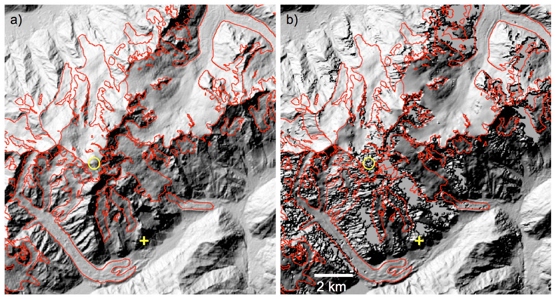
Figure 2 Comparison of hillshade views from (a) the AW3D30 DEM and (b) the TanDEM-X DEM for a region around Mont Blanc (Monte Bianco). Glacier outlines are shown in red, and data voids in the TanDEM-X DEM are depicted as constantly grey areas. The yellow circle marks the Mont Blanc summit, and the yellow cross in the lower centre marks the coordinates 45.8^∘ N and 6.9^∘ E. The AW3D30 DEM was downloaded from https://www.eorc.jaxa.jp/ALOS/en/aw3d30/index.htm (last access: 24 July 2019) and is provided by JAXA. The TanDEM-X DEM has been acquired by the TerraSAR-X/TanDEM-X mission and is provided by DLR (DEM_GLAC1823).

3.3 Previous glacier inventories

Outlines from previous national glacier inventories were used to guide the delineation. They have been mostly compiled from aerial photography with a spatial resolution better than 1 m and should thus provide the highest possible quality. This allowed considering very small and otherwise unnoticed glaciers and helped to identify glacier zones that are debris covered. The substantial glacier retreat that took place between the two inventories was well visible in most cases and did not hamper the interpretation. However, a larger number of mostly very small glaciers were either not mapped in 2003 and have now been added or were smaller in 2003 and now have larger extents. A large issue with respect to the additional workload is the compilation of ice divides. They can be derived semi-automatically from watershed analysis of a DEM using a range of methods (e.g. Kienholz et al., 2013), but in general many manual corrections still have to be applied. To have consistency with previous national inventories, we decided to use the drainage divides from these inventories to separate glacier complexes into entities. However, due to the locally poor geolocation of S2 scenes in steep terrain (Kääb et al., 2016; Stumpf et al., 2018), some ice divides of the former inventories overlapped with glacier extents (by up to 50 m) and were manually adjusted.

4 Methods

4.1 Mapping of clean ice in all regions

Automated mapping of clean to slightly dirty glacier ice is straightforward using a red or NIR to SWIR band ratio and a (manually selected) threshold (e.g. Paul et al., 2002). Other methods such as the normalized difference snow index (NDSI) also work well (e.g. Racoviteanu et al., 2009), as both utilize the strong difference in reflectance from the VNIR to the SWIR for snow and ice (e.g. Dozier, 1989). As the latter are bright in the VNIR bands (high reflectance) but very dark (low reflectance) in the SWIR, dividing a VNIR band by a SWIR band gives high values over glacier ice and snow and very low values over all other terrain, as this is often much brighter in the SWIR than the VNIR. The manual selection of a threshold for each scene (or S2 tile) has the advantage of including a regional adjustment of the threshold to local atmospheric conditions. We followed the recommendation to select the threshold in a way that good mapping results in regions with shadow are achieved. By lowering the threshold, more and more rock in shadow is included, creating a noisy result. It has been shown by Paul et al. (2016) that glacier mapping with S2 (using a red ∕ SWIR ratio) requires an additional threshold in the blue band to remove misclassified rock in shadow (that can have the same ratio value as ice in shadow but is darker in the blue band). Hence, for this inventory glaciers have first been automatically identified using the following equation:

$$\left(\mathrm{red}/\mathrm{SWIR}\right)>{\mathrm{th}}_{\mathrm{1}}\text{and blue}>{\mathrm{th}}_{\mathrm{2}},$$

with the empirically derived thresholds th₁ and th₂. As mentioned above, the SWIR band was bilinearly resampled from 20 to 10 m spatial resolution before computing the ratio. No filter for image smoothing was applied to retain fine spatial details, such as rock outcrops. Figure 3 shows the impact of the threshold selection for a test site in the Mont Blanc region (Leschaux Glacier). Figure 3a depicts the (contrast-stretched) red ∕ SWIR ratio image, Fig. 3b shows the impact of th₁ on the mapped area, Fig. 3c shows the impact of th₂, and Fig. 3d shows the resulting outlines after raster–vector conversion. As can be seen in Fig. 3b, there is very little impact on the mapped glacier area when increasing th₁ in steps of 0.2. For this region we used 3.0 as th₁, resulting in the blue and yellow areas being the mapped glacier. Wrongly mapped rock in shadow is then reduced back with th₂ (Fig. 3c) that is selected by visual analysis and expert judgement. In this case, a value of 860 was selected for th₂; i.e. only the blue area in Fig. 3c is considered. This removed rock in shadow from the glacier mask for the region to the right of the white arrow, but, on the other hand, correctly mapped ice in shadow is removed at the same time in the region above the green arrow (Fig. 3c and d). Hence, threshold selection is always a compromise as it is in general not possible to map everything correctly with one set of thresholds. In the resulting binary glacier maps, the “non-glacier” class is set to “no data” before being converted to a shape file using raster–vector conversion. In the resulting shape file, internal rocks are thus data voids.

Figure 3 Results of the automated (clean ice) glacier mapping and threshold selection: (a) band ratio MSI band 4 ∕ MSI band 11 (red ∕ SWIR). (b) Glacier classification results using different thresholds. The lower values add some additional pixels, in particular in shadow regions where the threshold is most sensitive. (c) Blue band threshold to remove wrongly classified rock in shadow. The highest value has been used, resulting in a good performance in the left part of the image (white arrow) and a bad one to the right (green arrow), where correctly classified ice in shadow is removed. (d) Final outlines (light blue) on top of the Sentinel-2 image in natural colours. The yellow cross to the lower right of the centre of panel (a) is marking the coordinates 45.87^∘ N and 7.0^∘ E (image source: Copernicus Sentinel data 2015).

All preprocessed scenes were provided in their original geometry for correction by the national experts. As shown in Fig. 3c, it was sometimes not possible to include dark bare ice and at the same time exclude bare rock in shadow. Such wrongly classified regions, together with data gaps for debris cover and clouds (omission errors), wrongly mapped water bodies (e.g. turbid lakes and rivers), and shadow regions (commission errors), were corrected by the analysts. By setting the minimum glacier size to 0.01 km², most of the often very small snow patches (i.e. <0.01 km²) were removed (cf. Leigh et al., 2019).

4.2 Corrections in the different countries

4.2.1 Austria

The satellite scenes for Austria were further preprocessed by Gabriele Schwaizer (cf. Paul et al., 2016) to remove water surfaces and improve classification of glacier ice in cast shadow before manual corrections were applied. The latter work was mainly performed by one person (Johanna Nemec). Two previous Austrian glacier inventories (Lambrecht and Kuhn, 2007; Fischer et al., 2015) were used to support the interpretation of small glaciers, debris-covered glacier parts, and the boundary across common accumulation areas. Further, an internal independent quality control of the generated glacier outlines was made by a second person (Gabriele Schwaizer), using orthophotos (30 cm resolution) acquired in late August 2015 for most Austrian glaciers for overall accuracy checks and to assure the correct delineation of debris-covered glacier areas. In Fig. 4a, we illustrate the strong glacier shrinkage from 1998 (yellow lines) to 2016 (red), as well as the manual corrections applied, extending the brightly filled areas of the raw classification to the red extents.

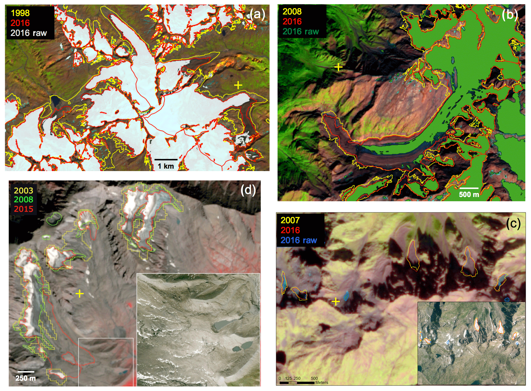
Figure 4 Examples of challenging classifications in different countries. (a) Debris cover delineation (red) around Grossvenediger (Hohe Tauern) in Austria with raw extents (light grey) and outlines from the previous national inventory (yellow). (b) Tré-La-Tête Glacier (Mont-Blanc), with automatically derived glacier extents (green), manually corrected outlines from 2015 (red), and outlines derived from aerial photographs taken in 2008 (yellow). The S2 image from August 2015 is in the background. (c) A subset of the Orobie Alps in Italy (S2 image from September 2016), with evidence of topographic shadow and debris-covered glaciers. The inset shows an aerial photograph with better glacier visibility but seasonal snow. (d) S2 image from 2015 showing differences in interpretation of debris cover for Gavirolas Glacier in Switzerland for the inventories from 2003 (yellow), 2008 (green), and 2015 (red). The inset shows a close-up of its lowest debris-covered part obtained from aerial photography for comparison (this image is a screenshot from Google Earth). The yellow crosses in each panel mark the following geographic coordinates: (a) 47.12^∘ N, 12.4^∘ E; (b) 45.8^∘ N, 6.75^∘ E; (c) 46.09^∘ N, 10.07^∘ E; and (d) 46.86^∘ N, 9.06^∘ E (image source: Copernicus Sentinel data 2015 and 2016).

4.2.2 France

The raw glacier outlines from S2 were corrected by one person (Antoine Rabatel). The glacier outlines from the previous inventory by Gardent et al. (2014) were used for the interpretation, in particular in shadow regions and for glaciers under debris cover. It is noteworthy that the previous inventory was made on the basis of aerial photographs (2006–2009) with field campaigns for the debris-covered glacier tongues to clarify the outline delineation. As a consequence, this previous inventory constitutes a highly valuable reference. In addition, because even on debris-covered glaciers the changes between 2006–2009 and 2015 are visible (Fig. 4b), Pléiades images from 2015–2016 acquired within the KALIDEOS-Alpes–CNES programme were used as a guideline, mostly for the heavily debris-covered glacier tongues.

4.2.3 Italy

As mentioned above, clouds covered the southern Alpine sector on the S2 scenes from August 2015. Hence, most of the inventory was compiled based on images from 2016, and three scenes from 2017 (see Table 1) were used to map glaciers under clouds or with adverse mapping conditions, i.e. excessive snow cover or shadows in the other scenes. Images acquired in August 2016 had little residual seasonal snow and a high solar elevation at the time of acquisition, which minimized shadow areas and created very good mapping conditions. In September 2016 and October 2017, more snow was present on high mountain cirques and glacier tongues, but comparatively few snow patches were found outside glaciers. However, the lower solar elevation compared to August caused a few north-facing glaciers and glacier accumulation areas to be under shadow. The raw glacier outlines from S2 were corrected by two analysts (Davide Fugazza and Roberto Sergio Azzoni). The outlines were separated into regions based on the administrative division of Italy, following the previous Italian glacier inventory (Smiraglia et al., 2015). Seasonal snow and rocks in shadow that were wrongly identified as clean ice, as well as lakes and large rivers, were manually deleted by the analysts. In shadow regions and for glaciers with large debris cover, the outlines from the previous Italian inventory by Smiraglia et al. (2015) were particularly valuable as a guide. Where some small glaciers were entirely under shadow, the outlines from the previous inventory were copied without changes, while in cases of partial shadow coverage they were edited in their visible portions. Due to the comparably small area changes of such glaciers over time, the former outlines are likely more precise than a new digitization under such conditions (cf. Fischer et al., 2014).

Glaciers in the Orobie Alps (ID 12 in Fig. 1), Dolomites, and Julian Alps (ID 18) posed significant challenges for glacier mapping. The three regions host very small niche glaciers and glacierets: in the Orobie and Julian Alps, their survival is granted by abundant snowfall, northerly aspect, and accumulation from avalanches, with debris cover also playing an important role. In the Dolomites, debris cover is often complete (Smiraglia and Diolaiuti, 2015), while the steep rock walls provide shadow and further complicate mapping. For glaciers in the Orobie Alps, an aerial orthophoto acquired by Regione Lombardia (https://www.geoportale.regione.lombardia.it, last access: 20 June 2020) in 2015 was used to aid the interpretation in view of its finer spatial resolution (e.g. Fischer et al., 2014; Leigh et al., 2019), although the image also shows evidence of seasonal snow. Here, manual delineation of the glacier outlines was required, as the band ratio approach could only detect small snow patches (see Fig. 4c). In the other two regions, outlines from the previous inventory, derived from aerial orthophotos acquired in 2011, were copied and only corrected where evidence of glacier retreat was found. Whereas the uncertainty in the outlines of the latter glaciers can be large (some of them are marked as “extinct” in the first Italian inventory from 1959 to 1962), the combined glacier area from the three regions is just above 1 % (1.35 km²) of the total area of Italian glaciers. For several of these very small, partly hidden entities, one can certainly discuss if they should be kept at all. In this inventory, they have been included for consistency with the last national inventory.

4.2.4 Switzerland

The raw glacier outlines from S2 were corrected by three people (Raymond Le Bris, Frank Paul, and Philipp Rastner), each of them being responsible for a different main region (south of the Rhône, north of the Rhône and Rhine, and south of the Rhine). The glacier outlines from the previous inventory by Fischer et al. (2014) were highly valuable for the interpretation, in particular in shadow regions and for glaciers under debris cover. In the hot summer of 2015, most seasonal snow had disappeared by the end of August, and thus mapping conditions with a comparably high solar elevation (limited regions in shadow) were very good. Some glaciers that could not be identified in the (contrast-stretched) S2 images were either copied from the previous inventory (if located in shadow) or assumed to have disappeared (if sunlit). Wrongly mapped (turbid) lakes and rivers (Rhône, Aare) were manually removed.

In a few cases (mostly debris-covered glaciers), we had to deviate from the interpretation of the previous inventories. As shown in Fig. 4d, very high-resolution satellite imagery or aerial photography (as available in Google Earth or from map servers) do not always help in finding a “correct” interpretation of glacier extents, as the rules applied for identification of ice under debris cover might differ (see Figs. S1, S2 and S3 in the Supplement). In this case it seems that the debris-covered region was not corrected in the 2003 and 2008 inventories, but it is now included (one can still discuss the boundaries). The interpreted glacier area has thus grown strongly since 2003 due to the better visibility of debris cover with S2.

4.3 Drainage divides and topographic information

Drainage divides between glaciers were copied from previous national inventories but were locally adjusted along national boundaries. In part this was required because different DEMs had been used in each country to determine the location of the divide. Additionally, some glaciers are divided by national boundaries rather than flow divides. This can result in an arbitrary part of the glacier (e.g. its accumulation zone) being located in one country and the other part (e.g. its ablation zone) being located in another country. As this makes no sense from a glaciological (and hydrological) point of view, such glaciers (e.g. Hochjochferner in the Ötztal Alps) have been corrected in such a way that they belong to the country where the terminus is located. There are thus a few inconsistencies in this inventory compared to the national ones.

After digital intersection of glacier outlines with drainage divides, topographic information for each glacier entity is calculated from both DEMs (ALOS and TDX) following Paul et al. (2009). The calculation is fully automated and applies the concept of zone statistics introduced by Paul et al. (2002). Each region with a common ID (this includes regenerated glaciers consisting of two polygons) is interpreted as a zone over which statistical information (e.g. minimum, maximum, and mean elevation) is derived from an underlying value grid (e.g. a DEM or a DEM-derived slope and aspect grid). Apart from glacier area (in km²), all glaciers have information about mean, median, maximum, and minimum elevations; mean slope and aspect (both in degrees); and aspect sector (eight cardinal directions) using letters and numbers (N =1, NE =2, etc.). Further information that is appended to each glacier in the attribute table of the shape file is as follows: the satellite tile used, the acquisition date, the analyst, and the funding source. This information is applied automatically by digital intersection (“spatial join”) to all glaciers from a manually corrected scene footprint shape file (see Fig. 1). The various attributes have then been used for displaying key characteristics of the datasets in bar graphs, scatter plots, and maps (see Sect. 5.1).

4.4 Change assessment

Glacier area changes have only been calculated with respect to the inventory from 2003, as the dates for the previous national inventories were too diverse for a meaningful assessment (see Sect. 1). To obtain consistent changes, only glaciers that are also mapped in the 2003 inventory are used for a direct comparison (automatically selected via a “point in polygon” check). However, after realizing that a glacier-specific comparison is not possible due to differences in interpretation (caused by the higher resolution of S2 and the different national rules) and changes in topology (e.g. inclusion of tributaries that were separated in 2003), we decided to only compare the total glacier area of the previous and new inventory.

4.5 Uncertainty assessment

As several analysts have digitized the new inventory, we performed multiple digitizings of a preselected set of glaciers to determine internal variability in interpretation per participant and across participants as a measure of the uncertainty of the generated dataset. For this purpose, all participants used the same raw outlines from S2 tile 32TLR (no. 23 in Fig. 1) to manually correct 14 glaciers (sizes from 0.1 to 10 km²) to the south of Lac des Dix around Mont Blanc de Cheilon (3870 m a.s.l.) for debris cover. All glaciers had to be digitized four times by five participants, giving a nominal total of 280 outlines for comparison. Results were analysed using an overlay of outlines to identify the general deviations in interpretation and through a glacier-by-glacier comparison of glacier sizes. For the latter, all datasets were intersected with the same drainage divides and glacier-specific areas were calculated. For each glacier and the entire region, mean area values and standard deviations are calculated per glacier, per participant, and for the total sample. The participants were asked to only use the S2 image and the 2003 outlines as a guide for interpretation in the first two digitization rounds and consider interpretation of very high-resolution imagery as provided by Google Earth for the second two rounds. At a minimum, 1 day should have passed between each digitization round and no former outlines were allowed to be shown. On average, each digitization round took about 2 h.

Additionally, we applied the buffer method (e.g. Paul et al., 2017) to obtain a statistical uncertainty value for the entire sample. This method gives a minimum and maximum area and was used to determine a relative area difference. This value multiplied by 0.68 gives the standard deviation (assuming normally distributed deviations from the correct outline) that is used as a further measure of area uncertainty (Paul et al., 2017). The selected buffer is based on an earlier multiple digitizing experiment for a couple of glaciers (Paul et al., 2013), showing that the variability in the positioning is within one pixel (or about ±10 m in the current case) of both sides of the “true” vector line. Strictly, a larger buffer should be used for the debris-covered glacier parts, as their uncertainty is higher. However, we have not implemented this here, as the related calculations are computationally expensive (cf. Mölg et al., 2018) and would still not reflect the real problem in debris identification as shown in Fig. 4d. Instead, we additionally applied a ±2 pixels buffer to all glaciers. For the majority of the debris-covered glaciers (i.e. those where debris can at least be identified) this gives an upper-bound value of the uncertainty. Depending on the degree of debris cover along the perimeter, the uncertainty is between the two values derived from the two buffers.

5 Results

5.1 The new glacier inventory

In total, we identified 4395 glaciers larger than 0.01 km², covering a total area of 1805.9 km², of which 361.5 km² (20 %) is found in Austria and 227.1 (12.6 %), 325.3 (18 %), and 892.1 km² (49.4 %) is found in France, Italy, and Switzerland, respectively. The size class distribution by area and count is depicted in Fig. 5a and is also listed in Table 2. In total, 62.5 % (92 %) of all glaciers are smaller than 0.1 km² (1.0 km²), covering 5.5 % (28 %) of the glacierized area, whereas 1.6 % are larger than 5 km² and cover 40 %. Thereby, glaciers in the size class 1 to 5 km² alone cover one-third (31.5 %) of the area but only 6.4 % of the total number. This biased size class distribution is typical for alpine glaciers where a few large glaciers are surrounded by numerous much smaller ones. The distribution of glacier number and area by aspect sector displayed in Fig. 5b shows the dominance, both in number and coverage area, of northerly exposed glaciers compared to all other sectors. About 60 % of all glaciers (covering 60 % of the area) are exposed to the NW, N, or NE, whereas only 21 % of all glaciers are found in the SE, S, and SW sectors. This distribution of glacier aspects is typical for regions where radiation plays a larger role in glacier existence compared to factors such as precipitation (Evans and Cox, 2005). The larger area coverage for glaciers facing SE is mostly due to the large Aletsch and Fiescher glaciers.

Table 2 Glacier area and count per size class for the entire sample.

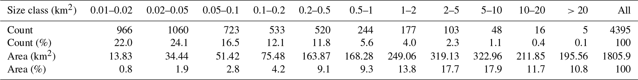
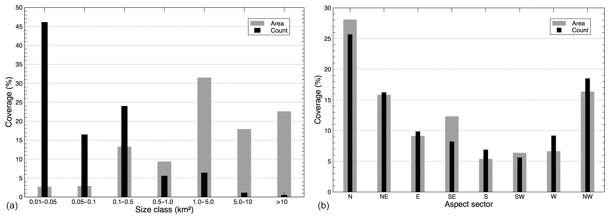
Figure 5 Relative frequency histograms for glacier count and area per (a) size class and (b) aspect sector for all glaciers.

A plot of glacier surface area vs. minimum and maximum elevations (Fig. 6a) reveals that glaciers smaller than 1 km² cover nearly the full range of possible elevations, indicating that their mean elevation is also impacted by factors other than climate (i.e. they can also exist at low elevations when they are located in a well-protected environment). Glaciers larger than 1 km², on the other hand, have clearly distinguished maximum and minimum elevations, i.e. they arrange around a climatically driven mean elevation that is around 3000 m a.s.l. Plotting glacier area vs. elevation range (Fig. 6b) shows that the largest glaciers are not those with the highest elevation range (the maximum of 3140 m is for Glacier des Bossons in the Mont Blanc massif with a size of 10 km²) and that for the majority of glaciers the elevation range increases with glacier size. This is typical for regions dominated by mountain and valley glaciers, as these follow the given topography. The ca. 7 km² Plaine Morte Glacier is a plateau glacier with an elevation range of only 350 m and represents an exception from the rule that larger glaciers generally have a larger elevation range.

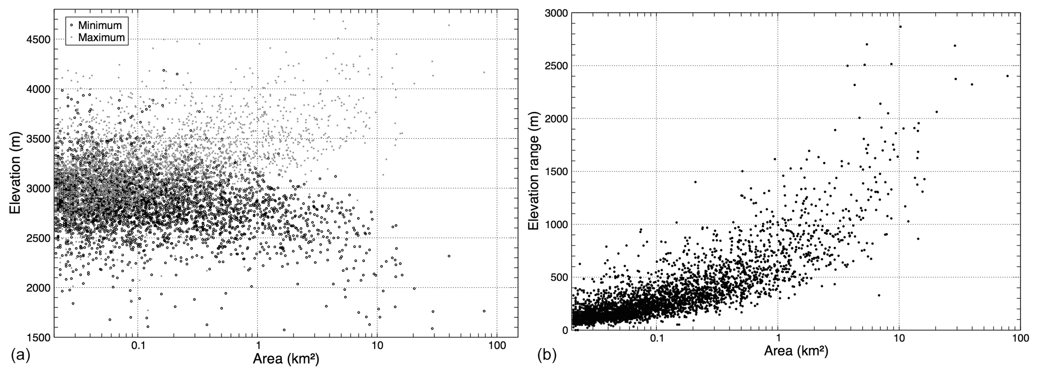
Figure 6 Glacier area vs. (a) minimum and maximum elevation and (b) elevation range for all glaciers.

The median elevation of a glacier is largely driven by temperature, precipitation, and radiation receipt (which depends on topography). As temperature is rather similar at the same elevation over large regions (e.g. Zemp et al., 2007) and topography (aspect and shading) has a strong local impact on radiation receipt, the large-scale variability of median (or mean) elevation of a glacier has a high correlation with precipitation (e.g. Ohmura et al., 1992; Oerlemans, 2005; Rastner et al., 2012; Sakai et al., 2015). The spatial distribution of glacier median elevations in the Alps (Fig. 7) thus also reflects the general pattern of annual precipitation amounts (e.g. Frei et al., 2003). When focusing on glaciers larger than 0.5 km² (that are less impacted by local topographic conditions), clearly lower median elevations (around 2400 m a.s.l.) are found for glaciers along the northern margin of the Alps and major mountain passes than in the inner Alpine valleys (around 3700 m a.s.l.) that are well shielded from precipitation. On top of this variability is the variability due to a different aspect (Fig. 7, inset): on average, glaciers that are exposed to the south have median elevations that are about 250 m higher (mean 3125 m a.s.l.) than north-facing glaciers (mean 2875 m a.s.l.). However, the scatter is high, and for each aspect the elevation variability is about 1500 m.

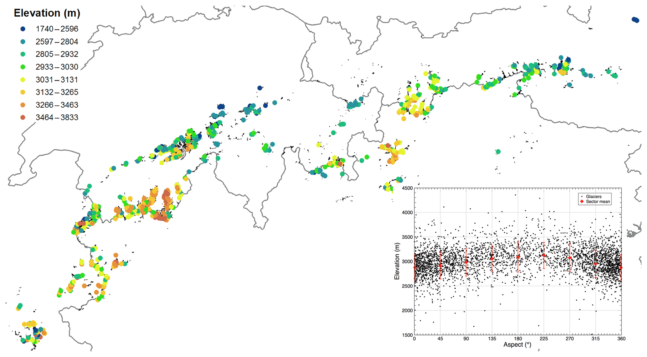
Figure 7 Spatial distribution of median elevation (colour-coded) for glaciers larger 0.5 km². The inset shows a scatterplot depicting glacier aspect (counted from north at 0^∘) vs. median elevation and values averaged for each cardinal direction.

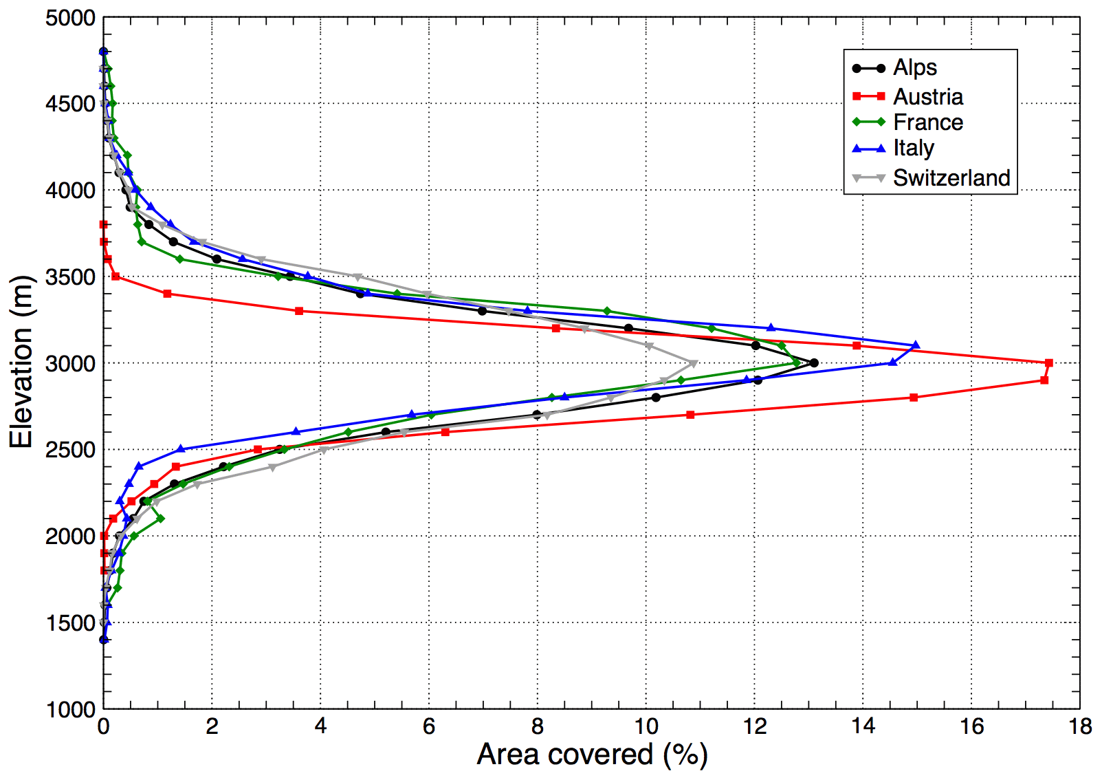
The graph in Fig. 8 shows the hypsometry of glacier area in the four countries and for the total area in relative terms. On average, the highest area share is found around the mean elevation of 3000 m a.s.l. By referring to the total area as 100 % for each country, differences among them can be seen. Most notable is the smaller elevation range and larger peak of glaciers in Austria, the broader vertical distribution in Switzerland (with the lowest peak value), and the slightly higher peak of the distribution in Italy (at 3100 m a.s.l). The hypsometry of glaciers in France is closest to the curve for the entire Alps.

Figure 8 Normalized glacier hypsometry per country as derived from the AW3D30 DEM.

5.2 Area changes

For a selection of 2873 comparable polygon entities present in both inventories, total glacier area shrunk from 2060 km² in 2003 to 1783 km² in 2015/16, i.e. by −13.2 % (−1.1 % a⁻¹). Considering the assumed missing area in the 2003 inventory of about 40 km² (glaciers with area gain are 29.4 km² larger in 2015/16 than in 2003), a more realistic area loss is −15 % or −1.3 % a⁻¹. This is about the same pace as reported earlier by Paul et al. (2004) for the Swiss Alps from 1985 to 1998/99 (−1.4 % a⁻¹). An example of the strong glacier shrinkage in Austria is depicted in Fig. 9. Closer inspection of this image also reveals a small shift (about up to 50 m to the SE) of the S2 scenes compared to the earlier Landsat TM scenes.

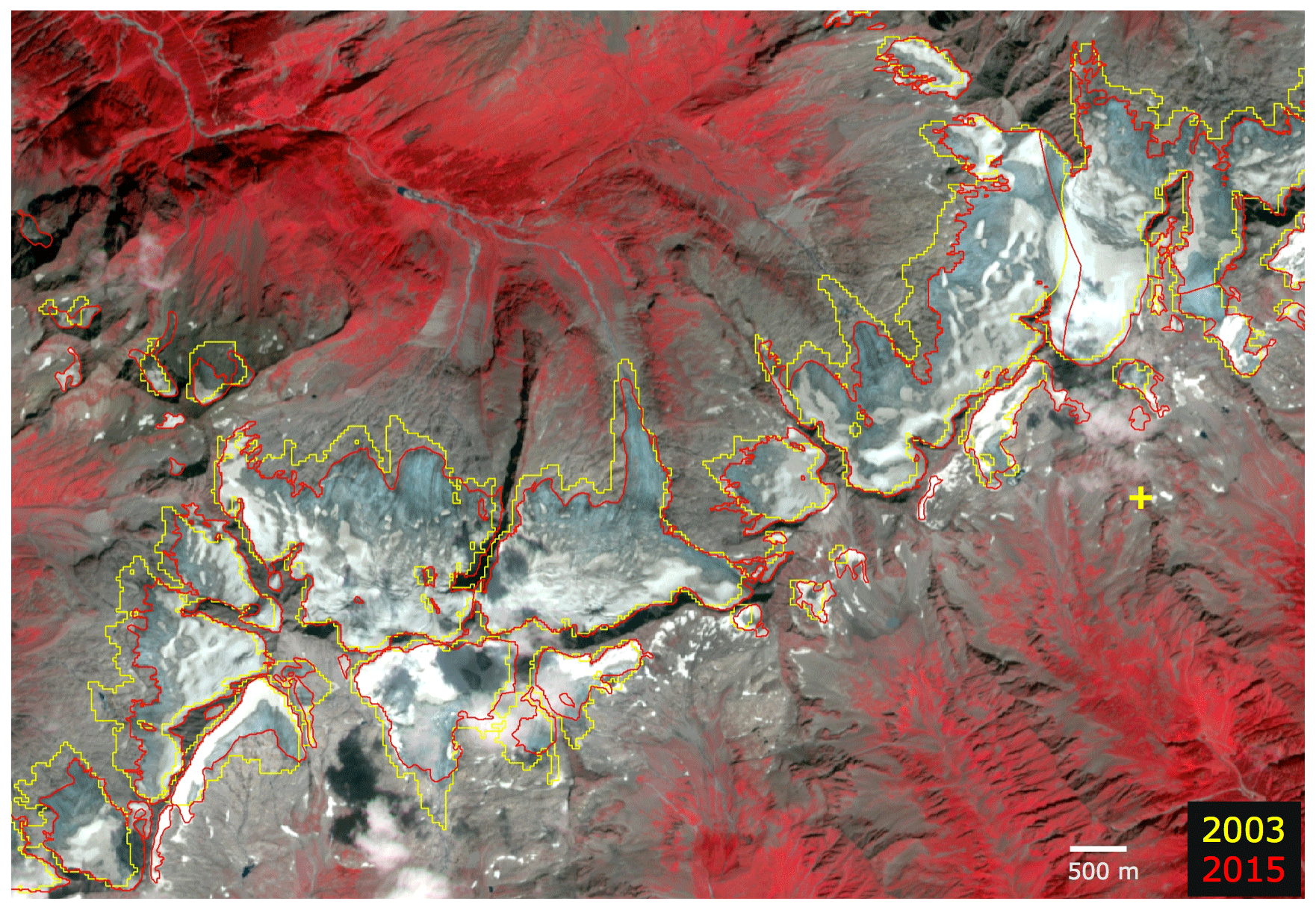
Figure 9 Visualization of the strong glacier area shrinkage between 2003 (yellow) and 2015 (red) for a subregion of the Zillertal Alps (Austria and Italy). The yellow cross on the right marks the coordinates 47.0^∘ N, and 11.88^∘ E (image source: Copernicus Sentinel data 2015).

The comparison of glacier outlines in Fig. 10 illustrates, for the region around Sonnblickkees in Austria, why we do not provide a scatterplot of relative area changes vs. glacier size or country-specific area change values (cf. also Fig. 4d for Gavirolas Glacier in Switzerland). Due to the different interpretations in the new inventory, 125 mostly very small glaciers are 100 % to 630 % larger than in 2003 and a large number (557) are 0 % to 100 % larger. For example, the 4 km² Suldenferner has increased in size by 550 %, as a small tributary (that holds the ID for the glacier) was disconnected in 2003 but is now connected to the entire glacier. Although such cases can be manually adjusted, it would not solve the general problem of differing interpretations when using data sources with differing spatial resolutions (cf. Fischer et al., 2014; Leigh et al., 2019). For example, the glacier in Fig. 4d has increased its size from 2003 to 2015 by 56 % due to the new interpretation. On the other hand, Careser Glacier, which fragmented into six ice bodies from 2003 to 2015, lost 55 % of its area when summing up all parts, as opposed to 63 % when considering the largest glacier only. As a consequence, the possible area reduction due to melting is partly compensated by the more generous interpretation of glacier extents and thus is of limited meaning for individual glaciers. Overall, glacier extents in the 2015/16 inventory might be somewhat larger than in reality due to the inclusion of seasonal or perennial snow in some regions. The −15 % area loss mentioned above can thus be seen as a lower-bound estimate.

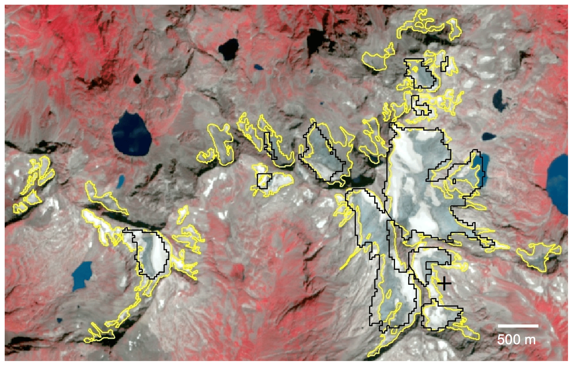
Figure 10 Overlay of glacier outlines from 2003 (black) and 2016 (yellow) showing the different interpretation of glacier extents for the region around Sonnblickkees (SBK) in Austria. The black cross on the lower right marks the coordinates 47.12^∘ N, 12.6^∘ E (image source: Copernicus Sentinel data 2015).

5.3 Uncertainties

5.3.1 Glacier outlines

The multiple digitizing experiment revealed several interesting (albeit well-known) results. Overall, the area uncertainty (1 standard deviation, SD) is 3.3 % across all participants for the total of the digitized area (Table 3). As two glaciers (11 and 13) were not mapped by one participant, the missing values are replaced with the mean value from the other participants. Across all glaciers, but for individual participants, the uncertainty (comparing the values from the four digitization rounds) is lower (1 % to 2.7 %), indicating that the digitizing is more consistent when performed by the same person. The area values of participant 1 (P1) are systematically higher than for the other participants, about 6 % for the total area. A detailed analysis (close-ups and only showing individual datasets) of the digitized outlines (Fig. 11) revealed that the differences are mostly due to the more generous inclusion of debris-covered glacier ice for two of the larger glaciers (nos. 1 and 5). When excluding P1, the SD across the other participants is 3 times smaller (1.1 %). The uncertainty also slightly depends on glacier size, showing values between 1 % and 6 % for glaciers larger than 1 km² and between 2 % and 20 % for glaciers <1 km². The smallest glacier in the sample is smaller than 0.1 km² and shows variations in SD between 8 % and 44 %, in the latter case this is also due to a reinterpretation of its extent when using very high-resolution imagery. For such small glaciers, related changes can thus result in considerably different extents.

Table 3 Results of the multiple digitizing experiment, listing for each of the five participants the mean glacier area (in km²) in the columns P1 to P5, along with the standard deviation in percent (SD %). The last two columns provide the averaged values across all participants for each glacier and the last row gives total areas and their standard deviation across all glaciers and for each participant. The two values marked in bold are mean values derived from the other four participants. In the last column, values in italic mark highest values for glaciers larger and smaller than 1 km². Glacier ID 4 is missing as it was digitized as one glacier (with ID 5) by most participants.

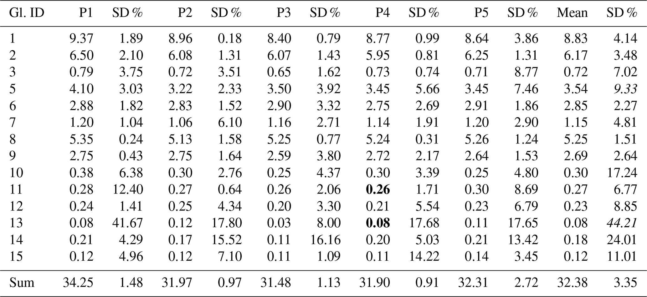
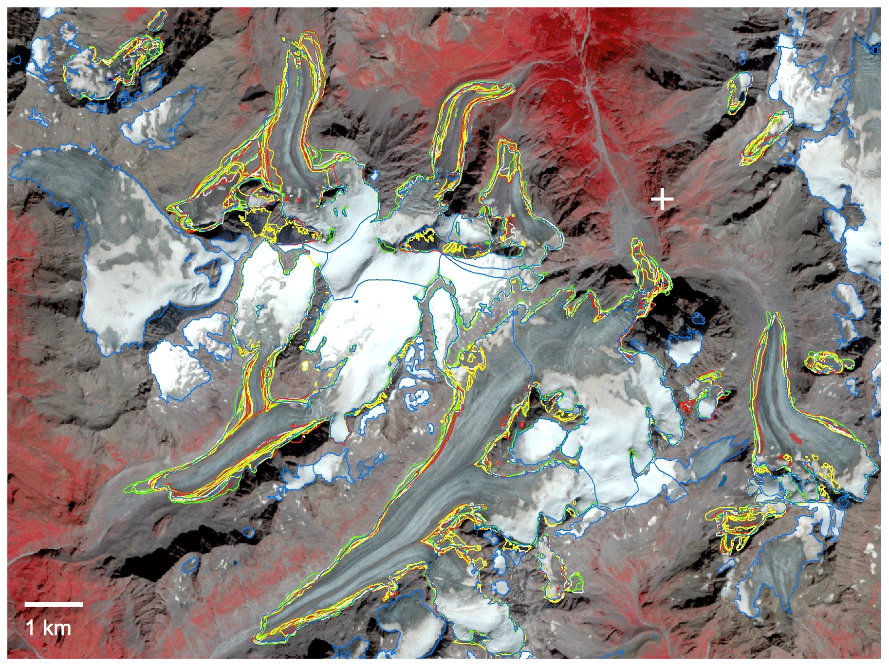
Figure 11 Overlay of glacier outlines from the multiple digitizing experiment by all participants. Colours refer to the first (yellow), second (red), third (green), and fourth (white) rounds of digitization. The white cross on the upper right marks the coordinates 46.0^∘ N, 7.5^∘ E (image source: Copernicus Sentinel data 2015).

Moreover, for P1 and most of the other participants, the digitized glacier extents increased by several percent after consultation of very high-resolution satellite images, e.g. those available from Google Earth and the Swisstopo map server (Supplement, Fig. S1). The generally very flat and debris-covered regions were barely visible on the S2 images and have been digitized differently in each of the four rounds. Hence, the possibility for a reinterpretation of the outlines within the same experiment resulted in higher standard deviations. Whether such regions have to be included in a glacier inventory or not can be discussed, as the transition to ice-cored medial or lateral moraines is often gradual and including these features in a glacier inventory or not is a (personal) methodological decision. Figures S2 and S3 in the Supplement provide examples of the difficulties in interpreting such regions. Even at this high spatial resolution, the exact boundary of the two glaciers is not fully clear, and thus a large interpretation spread can be expected at lower resolution. However, in general it seems that the area of glaciers with debris-covered margins is still slightly underestimated at 10 m resolution. This confirms the earlier recommendation of double-checking all digitized glacier extents with such very high-resolution sensors, at least for the difficult cases (e.g. Fischer et al., 2014).

The uncertainty (1 SD) obtained with the buffer method is ±5 % (10 %) when using a 10 m (20 m) buffer. Considering that the former buffer might be a realistic uncertainty bound for clean ice and that the latter buffer might be realistic for debris-covered ice, the “true” uncertainty value would be between 5 % and 10 % and for individual glaciers would largely depend on the difficulties in identifying ice under debris. This is in line with the uncertainties derived from multiple digitizing and numerous previous studies.

5.3.2 Topographic information

The comparison of topographic parameters (minimum, maximum, and mean elevation and mean slope and aspect) revealed larger differences when derived from either the TDX or AW3D30 DEM, in particular towards smaller glaciers. These are more likely to be impacted by artefacts as they share a larger percentage of their total area (Fig. 2). Differences in mean slope and aspect are generally small but increase towards larger slope values for the former. This is in agreement with the general observations that DEM quality is reduced at steep slopes. Minimum elevation is slightly higher in the TDX DEM, which can be explained by glacier retreat between the acquisition dates (around 2009 for AW3D30 vs. around 2013 for TDX). However, a clearly lower mean elevation due an overall surface lowering of the glaciers could not be observed, indicating that the differences are in the uncertainty range. Apart from artefacts, the uncorrected radar penetration of the TDX DEM into snow and firn might play a role here as well.

6 Discussion

The derived size class distribution (Fig. 5) and topographic information are typical for glaciers in mid-latitude mountain ranges with numerous smaller glaciers surrounding a few larger ones (e.g. Pfeffer et al., 2014). Only 349 out of 4395 glaciers (8 %) are larger than 1 km² and nearly half of them (46 %) are smaller than 0.05 km² and cover 2.7 % of the area. It might be possible that many of the latter are no longer glaciers but are instead just perennial snow and firn patches. However, for consistency with earlier national glacier inventories they have been included. Mean elevation values do not depend on size for such “glaciers”, indicating that they can survive at different elevations and that precipitation amounts have a limited impact on their occurrence (e.g. if fed by avalanche snow). If they are well protected from solar radiation (e.g. by shadow or debris cover) such glaciers might persist for some time despite increasing air temperatures. Glacier mean elevation does not depend on glacier size but on glacier location with respect to precipitation sources, in particular for larger glaciers (Fig. 7). On top of this dependence is the variability with mean aspect (Fig. 7, inset).

Widespread glacier thinning over the past few decades and over steep terrain have lately resulted in interrupted profiles for several larger valley glaciers. Their lower parts are now no longer nourished by ice from above. These separated parts thus can not be named “regenerated glaciers”, but instead they melt away as dead ice. Strictly speaking, such lower dead ice bodies (that can persist due to debris cover for a very long time) should be excluded from a glacier inventory (Raup and Khalsa, 2007). However, for consistency with former inventories and their contribution to run-off, we included them here and used the same ID for both parts to obtain topographic information for the combined extent. Calculating this for the individual parts instead would result in related outliers and a more difficult analysis of trends. At best, such separated parts are identified with a flag in the attribute table, for example as a further extension to the “form” attribute (e.g. “4: Separated glacier part”) used in the RGI (RGI consortium, 2017). However, the differentiation from a regenerated glacier might sometimes be difficult.

Due to the differences in interpretation (Fig. 10), we have not compared the 2003 extents of individual glaciers directly with those from the new inventory but we compared only the total area of glaciers observed in both inventories. Considering the underestimated glacier area in 2003 (e.g. due to missing debris cover) and possibly overestimated sizes in 2015 (e.g. due to included snow), the pace of shrinkage (−1.3 % a⁻¹) has not changed compared to the earlier mid-1980s to 2003 period. This indicates that most glaciers have not yet reached a geometry that is compliant with current climate conditions, and they will thus continue shrinking in the future. This becomes also clear from the snow cover remaining near the end of the ablation period on the glaciers, covering barely 20 % to 30 % of the area (e.g. Figs. 9 and 11). Assuming a required 60 % coverage of their accumulation area, glaciers in the Alps have to lose another 50 % to 70 % of their area to again reach balanced mass budgets (Carturan et al., 2013). There are other regions in the world with similar high (or even higher) area loss rates such as the tropical Andes (e.g. Rabatel et al., 2013), but to a large extent this is also due to the smaller glaciers in this region. A realistic comparison across regions would only be possible when change rates of identical size classes are compared.

The multiple digitizing experiment (Fig. 11) revealed a large variability in the interpretation of debris-covered glaciers among the analysts but high consistency in the corrections where boundaries are well visible. Related area uncertainties can be high for very small glaciers (>20 %) but are generally <5 %. The area reduction derived here of about −15 % since 2003 is thus significant, but for small and/or debris-covered glaciers the area uncertainty can be similar to the change, making it less reliable. However, this strongly depends on the specific glacier characteristics and cannot be generalized to all small glaciers.

The gradual disappearance of ice under debris cover and the separation of low-lying glacier tongues on steep slopes are major problems for any glacier inventory created these days. We decided to reconnect disconnected glacier parts using their ID (to multi-part polygons) for consistency with earlier inventories. However, keeping them separated is another possibility, given that possible dead ice is clearly marked in the attribute table.

7 Data availability

The dataset can be downloaded from https://doi.org/10.1594/PANGAEA.909133 (Paul et al., 2019).

8 Conclusions

We presented the results of a new glacier inventory for the entire Alps derived from Sentinel-2 images from 2015 and 2016. In total, 4395 glaciers >0.01 km² covering an area of 1806±60 km² are mapped. This is a reduction of about 300 km² or −15 % (−1.3 % a⁻¹) compared to the previous Alpine-wide inventory from 2003. The pace of glacier shrinkage in the Alps has remained about the same since the mid-1980s, indicating that glaciers will continue to shrink under current climatic conditions. Due to the differences in interpretation, we have not performed a glacier-by-glacier comparison of area changes. The ongoing glacier decline also results in increasingly difficult glacier identification (under debris cover) and topological challenges for a database (when glaciers split). The former is confirmed by the results of the uncertainty assessment, showing a large variability in the interpretation of glacier extents when conditions are challenging. Despite the additional workload, we think this is the best way to provide an uncertainty value for such a highly corrected and merged dataset. In any case, the outlines from the new inventory should be more accurate than for 2003, as we here used the previous, high-quality national inventories as a guide for interpretation, performed corrections by the respective experts, and worked with the higher resolution of Sentinel-2 data that helped in identifying important spatial details.

The clean-ice mapping with the band ratio method is straightforward, but requires well-thought-out decisions on the two thresholds as they will always be a compromise. They should be tested in regions with ice in cast shadow and selected in a way that the workload for manual corrections is minimized. If a precise DEM is available, the required corrections of wrongly mapped ice in shadow can be reduced, as revealed by the further preprocessing for glaciers in Austria. However, reduced DEM quality and illumination differences can limit the benefits of a topographic normalization of the images. Due to the artefacts in the first version of the TanDEM-X DEM, we used the ALOS AW3D30 DEM to derive topographic information for each glacier despite the less good temporal agreement. To conclude, we had datasets with a much higher spatial resolution available for this inventory compared to the 2003 dataset, but for several reasons (e.g. debris cover, clouds, seasonal snow) the creation of glacier inventories from satellite data and a DEM remains a challenging task with a high workload and expert knowledge required.