Description of the multi-approach gravity field models from Swarm GPS data

Although the knowledge of the gravity of the Earth has improved considerably with CHAMP, GRACE, and GOCE (see appendices for a list of abbreviations) satellite missions, the geophysical community has identified the need for the continued monitoring of the time-variable component with the purpose of estimating the hydrological and glaciological yearly cycles and long-term trends. Currently, the GRACE-FO satellites are the sole dedicated provider of these data, while previously the GRACE mission fulfilled that role for 15 years. There is a data gap spanning from July 2017 to May 2018 between the end of the GRACE mission and start the of GRACE-FO, while the Swarm satellites have collected gravimetric data with their GPS receivers since December 2013.

We present high-quality gravity field models (GFMs) from Swarm data that constitute an alternative and independent source of gravimetric data, which could help alleviate the consequences of the 10-month gap between GRACE and GRACE-FO, as well as the short gaps in the existing GRACE and GRACE-FO monthly time series.

The geodetic community has realized that the combination of different gravity field solutions is superior to any individual model and set up the Combination Service of Time-variable Gravity Fields (COST-G) under the umbrella of the International Gravity Field Service (IGFS), part of the International Association of Geodesy (IAG). We exploit this fact and deliver the highest-quality monthly GFMs, resulting from the combination of four different gravity field estimation approaches. All solutions are unconstrained and estimated independently from month to month.

We tested the added value of including kinematic baselines (KBs) in our estimation of GFMs and conclude that there is no significant improvement. The non-gravitational accelerations measured by the accelerometer on board Swarm C were also included in our processing to determine if this would improve the quality of the GFMs, but we observed that is only the case when the amplitude of the non-gravitational accelerations is higher than during the current quiet period in solar activity.

Using GRACE data for comparison, we demonstrate that the geophysical signal in the Swarm GFMs is largely restricted to spherical harmonic degrees below 12. A 750 km smoothing radius is suitable to retrieve the temporal variations in Earth's gravity field over land areas since mid-2015 with roughly 4 cm equivalent water height (EWH) agreement with respect to GRACE. Over ocean areas, we illustrate that a more intense smoothing with 3000 km radius is necessary to resolve large-scale gravity variations, which agree with GRACE roughly at the level of 1 cm EWH, while at these spatial scales the GRACE observes variations with amplitudes between 0.3 and 1 cm EWH. The agreement with GRACE and GRACE-FO over nine selected large basins under analysis is 0.91 cm, 0.76 cm yr⁻¹, and 0.79 in terms of temporal mean, trend, and correlation coefficient, respectively.

The Swarm monthly models are distributed on a quarterly basis at ESA's Earth Swarm Data Access (at https://swarm-diss.eo.esa.int/, last access: 5 June 2020, follow Level2longterm and then EGF) and at the International Centre for Global Earth Models (http://icgem.gfz-potsdam.de/series/02_COST-G/Swarm, last access: 5 June 2020), as well as identified with the DOI https://doi.org/10.5880/ICGEM.2019.006 (Encarnacao et al., 2019).

1 Introduction

Swarm is the fifth Earth Explorer mission by the European Space Agency (ESA), launched on 22 November 2013 (Haagmans, 2004; Friis-Christensen et al., 2008). Its primary objective is to provide the best ever survey of the Earth's magnetic field and its temporal variations as well as the electric field of the atmosphere (Olsen et al., 2013). Swarm consists of three identical satellites, two flying in a pendulum formation (side by side, converging near the poles) at an initial altitude of about 470 km and one at an altitude of about 520 km, all in near-polar orbit. In addition to a sophisticated instrument suite for observing the geomagnetic and electric fields, the Swarm satellites are equipped with high-precision, dual-frequency Global Positioning System (GPS) receivers, star trackers, and accelerometers. Many recent studies and activities have shown the feasibility of observing the Earth's gravity field and its long-wavelength temporal variations with high-quality GPS receivers on board low-Earth orbit (LEO) satellites (Zehentner and Mayer-Gürr, 2014; Bezdek et al., 2016; Dahle et al., 2017). For Swarm, Teixeira da Encarnação et al. (2016) successfully demonstrated the observation of long-wavelength temporal gravity. They produced solutions using three different approaches and showed that their combination resulted in improved observability of time variable gravity, a principle that has been suggested in the frame of the initiative of the European Gravity Service for Improved Emergency Management (EGSIEM) (Jäggi et al., 2019) and demonstrated for gravity field solutions based on the Gravity Recovery and Climate Experiment (GRACE) (Jean et al., 2018).

An important driver for producing LEO GPS-based gravity field solutions is to guarantee long-term observation of mass transport in the Earth system. The geophysical community has identified the need for continued monitoring of time-variable gravity for estimating the hydrological and glaciological yearly cycles and long-term trends (Abdalati et al., 2018). The US–German GRACE mission (Tapley et al., 2004) was by far the most important space-borne global provider of the needed data for the period from April 2002 until July 2017. GRACE Follow-On (GRACE-FO) was launched in May 2018 and is expected to continue the high-quality observation of Earth's time-variable gravity field for at least 5 years (Flechtner et al., 2016). Thus a time gap exists between the GRACE and GRACE-FO missions, and, importantly, no missions have yet been selected for the post-GRACE-FO period. It can thus be claimed that the only guarantee for sustained observation of time-variable gravity from space is constituted by space-borne GPS receivers on LEO satellites. Moreover, the associated data can be used to fill the gap between the GRACE and GRACE-FO missions (be it with a different quality in terms of spatial and temporal resolution). The measurement of Earth's gravitational changes with Swarm is further motivated by (i) the need to increase the accuracy of global mass estimates in order to properly quantify global sea-level rise and (ii) the opportunity to provide independent estimates of temporal variations in low-degree coefficients, in particular related to C_2,0 and C_3,0, which are weakly observed by GRACE. Under this motivation, this paper aggregates a series of studies and analyses that, respectively, motivate our processing choices and demonstrate the capabilities of the combined Swarm models to observe mass transport processes at the surface of the Earth on a monthly basis, in a way that is superior to any of its individual models.

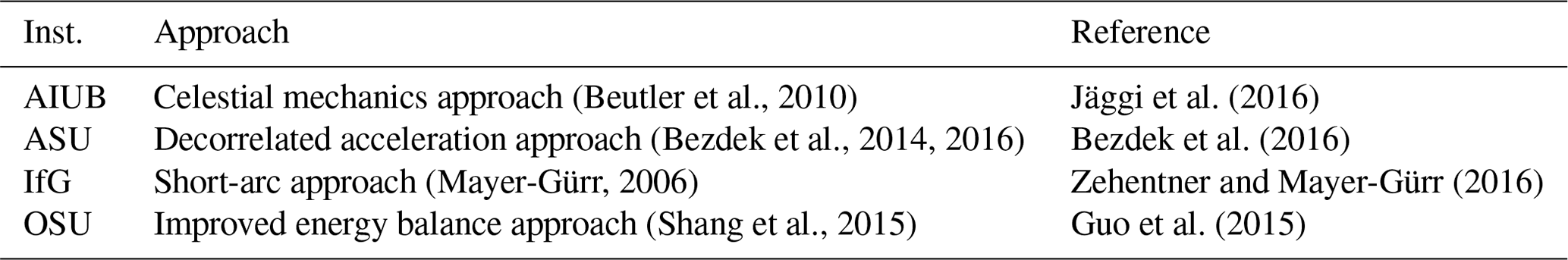
The studies aim at improving Swarm-based observation of long-wavelength time-variable gravity in support of the operational delivery of Swarm-based gravity field solutions. It is a continuation of the activities described in Teixeira da Encarnação et al. (2016), which included the production of gravity field solutions using three different methods, referred to as the celestial mechanics approach (CMA) (Beutler et al., 2010), decorrelated acceleration approach (DAA) (Bezdek et al., 2014), and short-arc approach (SAA) (Mayer-Gürr, 2006). In this work, a fourth method, referred to as the improved energy balance approach (IEBA) (Shang et al., 2015), is added. The combination of the four gravity field solutions into combined models will be more advanced than in Teixeira da Encarnação et al. (2016), where a straightforward averaging was applied. In the results presented in this work, the weights are derived from variance component estimation (VCE) analogously with Jean et al. (2018), in order to arrive as close as possible at statistically optimal combined solutions, given the available combination strategies, as described in Sect. 2.5.

The nominal gravity field solutions will be based on kinematic orbit (KO) solutions, which consist of time series of position coordinates. These time series can be considered a condensed form of the original GPS high–low satellite-to-satellite tracking (hl-SST) observations, with no effect from dynamic models for the LEO satellites (the positions of the GPS satellite themselves are based on dynamic models, as usual). Three different KO solutions are produced by the Delft University of Technology (TUD), Astronomical Institute of the University of Bern (AIUB), and the Institute of Geodesy Graz (IfG) of the Graz University of Technology (TUG) (van den IJssel et al., 2015; Jäggi et al., 2016; Zehentner, 2016).

We also tested another potential innovation that could conceptually lead to improved gravity field solutions, that is the use of kinematically derived baselines for the two Swarm satellites flying in a pendulum formation. Kinematic baselines (KBs) between two LEO formation-flying spacecraft can typically be derived with much better precision than the absolute positions by making use of ambiguity-fixing schemes and due to cancellation of common errors (Kroes, 2006; Allende-Alba et al., 2017). The possible added value of KBs for the observation of temporal gravity field variations will be assessed making use of two different KB solutions by TUD (Mao et al., 2017) and the AIUB (Jäggi et al., 2007, 2009).

We also present a comparison of the quality of gravity field retrievals from Swarm C observational data making use of either the available accelerometer product for this satellite (Doornbos et al., 2015) or two different non-gravitational acceleration force models.

This paper is organized as follows. More details about the methodology are provided in Sect. 2. Results are included and discussed in Sect. 3. A summary, conclusions, and outlook are given in Sect. 4.

For the sake of brevity, we will refer to GRACE and GRACE-FO data simply as GRACE data, unless there is the need to be more specific. We also interchangeably use the terms solution (when relevant to a set of Stokes coefficients) and gravity field model (GFM).

The operational activities currently under way pertaining to the combined models described in this article are conducted in the frame of the Combination Service of Time-variable Gravity Fields (COST-G), under the umbrella of International Gravity Field Service (IGFS) International Association of Geodesy (IAG) (Jäggi et al., 2020), with additional support from the Swarm Data, Innovation and Science Cluster (DISC) and funded by ESA. The Swarm monthly models are distributed on a quarterly basis at ESA's Earth Swarm Data Access (at https://swarm-diss.eo.esa.int/, last access: 5 June 2020, follow Level2longterm and then EGF) and at the International Centre for Global Earth Models (http://icgem.gfz-potsdam.de/series/02_COST-G/Swarm, last access: 5 June 2020), as well as identified with the DOI https://doi.org/10.5880/ICGEM.2019.006 (Encarnacao et al., 2019).

2 Methodology

In this work, we mainly intend to present the capabilities of the Swarm GFMs, in terms of their particularities and data quality, and we typically refer to the relevant methodology in supporting literature. Nevertheless, this section discusses briefly some aspects of the various stages in the processing of the models, their combination, and, to better prepare the discussion of results in Sect. 3, the approach used in the analysis of the Swarm GFMs.

2.1 Kinematic orbits

The KOs are the observations from which the GFMs are estimated, since they are solely derived from the geometric distance relative to the GPS satellites. The different KO solutions are conceptually estimated in similar ways, but with the processing strategies described in detail in the references of Table 1. Furthermore, each analysis centre (AC) makes their own choices regarding the numerous assumptions and processing options for deriving their individual KO solutions, as listed in Appendix A. The reason for the different KO solutions is to provide various options for the ACs' individual GFM processing (see Sect. 2.4) and, in this way, reduce the impact of possible KO-driven systematic errors in the combined GFMs. It also enables the ACs to select which KO solution is more advantageous to the quality of their GFMs; consider that our gravity estimation approaches may be differently sensitive to the error spectra of the various KO solutions or have different requirements on the quality of the variance–covariance information provided with the kinematic positions. This selection is done at each AC and outside the scope of the current study.

2.2 Kinematic baselines

We investigate the added value of KBs in the quality of the Swarm GFMs, as presented in Sect. 3.1. The KB solutions, much in the same way as the KOs, are conceptually computed similarly, where fixing ambiguities is a necessary processing step to achieve the highest possible precision of the derived baselines. This constitutes the main motivation to include KBs in the estimation of the Swarm GFMs. The interested reader can find details in the references of Table 2; the main processing assumptions are listed in Appendix B and brief descriptions follow.

Table 1 Overview of the kinematic orbits and the software packages used to estimate them.

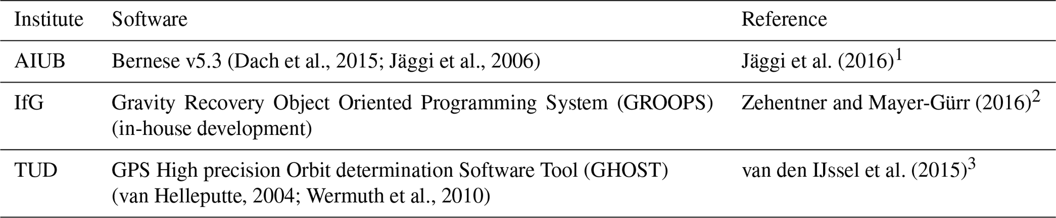
¹ ftp://ftp.aiub.unibe.ch/LEO_ORBITS/SWARM (last access: 5 June 2020). ² ftp://ftp.tugraz.at/outgoing/ITSG/tvgogo/orbits/Swarm (last access: 5 June 2020). ³ http://earth.esa.int/web/guest/swarm/data-access (last access: 5 June 2020).

Table 2 Overview of the kinematic baselines and the software packages used to estimate them.

2.2.1 KBs produced at AIUB

Kinematic and reduced-dynamic baselines are determined according to the procedures described by Jäggi et al. (2007, 2009, 2012). The positions of one satellite (Swarm A) are kept fixed to a reduced-dynamic solution generated from zero-differenced (ZD) ionosphere-free GPS carrier phase observations. Reduced-dynamic orbit parameters of the other satellite (Swarm C) are estimated by processing double-differenced (DD) ionosphere-free GPS carrier phase observations with DD ambiguities resolved to their integer values. First, the Melbourne–Wübbena linear combination is analysed to resolve the wide-lane ambiguities, which are subsequently introduced as known to resolve the narrow-lane ambiguities together with the reduced-dynamic baseline determination. For the KB estimation, the same procedure may be used but it turned out to be more robust to introduce the resolved ambiguities from the available reduced-dynamic baselines and not to make an attempt to independently fix carrier phase ambiguities in the KB processing. Exactly the same carrier phase ambiguities are therefore fixed in both the reduced-dynamic and the kinematic baseline determinations.

2.2.2 KBs produced at TUD

We take advantage of a forward and backward extended Kalman filter (EKF) that is run iteratively. The EKF initially runs from the first epoch to the last epoch of each 24 h orbit arc with 5 s step. The estimated float ambiguities and the corresponding covariance matrices (which are recorded for each epoch) are used by the least-squares ambiguity decorrelation adjustment (LAMBDA) algorithm in order to fix the maximum number of integer ambiguities (subset approach). The EKF smooths both solutions according to the bi-directional covariance matrices recorded at each epoch. In the next iteration, the smoothed orbit and fixed ambiguities are set as input and it is attempted to fix more ambiguities. The procedure is repeated until no new integer ambiguities are fixed.

After the convergence of the reduced-dynamic baseline, a KB solution is produced using the least-squares (LS) method. To this purpose, the same GPS observations and fixed integer ambiguities on the two frequencies are used, where one satellite (Swarm A) is kept fixed at the reduced-dynamic baseline solution. At least five observations are required on each frequency to form a good geometry. To minimize the influence of wrongly fixed ambiguities and residual outliers, a threshold of 2-sigma of the carrier phase residual standard deviation (SD) is set, which results in eliminating around 5 % of data, on average. A further screening of 3 cm is set to the rms of the kinematic baseline carrier phase observation residual. This makes it possible to screen out the epochs that are influenced by wrongly fixed ambiguities and bad phase observations. The kinematic baseline determination is also run bi-directionally to compute two solutions that are averaged according to the epoch-wise covariance matrices.

2.2.3 Inclusion of KBs in the estimation of Swarm GFMs

We exploit the variational equations approach (VEA) (Montenbruck and Gill, 2000) implemented at IfG in the inversion of gravity field considering both KOs and KBs. The VEA and its application to KOs and KBs corresponds to the processing scheme used for the production of the ITSG-Grace2016 (Klinger et al., 2016).

Table 3 Periods considered in the analysis of the added value of different types of non-gravitational accelerations.

We selected a number of suitable test months with varying data quality, meeting the following criteria: GRACE monthly solutions are available for validation purposes, months with good GPS data quality are included as well as months with bad data quality, and some months should overlap with the test months selected in the non-gravitational acceleration study (Sect. 2.3) for the accelerometer data tests.

The descriptions good and bad data quality refer to several issues in the context of Swarm GPS data. Good means that an error found in the Receiver Independent Exchange Format (RINEX) converter is solved (fixed since 12 April 2016), the settings of the receiver tracking loop bandwidths are optimized (several changes during lifetime), and the ionospheric activity is at a low level. In contrast, the bad data hold for time periods for which these issues are not solved and the ionospheric activity is high. Finally, the intermediate data are during periods of lower ionospheric activity (relative to early 2015) but before the GPS receiver updates. In total we have selected seven test months: January and March 2015 refer to bad data quality, February and March 2016 refer to intermediate data quality, and June–August 2016 refer to good data quality.

The existing software exploiting VEA at IfG handles the Swarm KB data under the same processing scheme and handling of stochastic properties of the observations adopted for the generation of the ITSG-Grace releases (Mayer-Gürr et al., 2016). The observations derived from the Swarm KBs are introduced into the gravity inversion process as if they were collected by the K-Band ranging instrument. Our software is not prepared to handle the full three-dimensional (3D) information of the KBs, and the development of this capability is outside the scope of this study.

The KBs and KO solution are selected consistently from the same AC (i.e. TUD or AIUB) when producing the gravity field solution. In total four different GFM variants have been computed: (1) hl-SST solution from TUD KOs, (2) hl-SST + low–low satellite-to-satellite tracking (ll-SST) solution from TUD KOs and KBs, (3) hl-SST solution from AIUB KOs, and (4) hl-SST + ll-SST solution from AIUB KOs and KBs. The four solution variants were produced for all seven test months.

2.3 Non-gravitational accelerations

We assessed the quality of the Swarm GFMs when the non-gravitational accelerations are modelled following two distinct approaches and when they are represented by the Level 1B (L1B) accelerometer data from Swarm C (Siemes et al., 2016). One non-gravitational acceleration model was produced at the Astronomical Institute Ondřejov (ASU) and the other at the Delft University of Technology (TUD). We selected a number of periods for our tests (see Table 3), taking care to cover as much as possible different accelerometer data variability (arising from instrument artefacts) and signal amplitude, as well as ionosphere and geomagnetic activity, to cover different regimes of non-gravitational accelerations acting on the Swarm satellites. Moreover, we also chose months when GRACE gravity field solutions are available, to facilitate validation of the Swarm GFMs.

For the ASU model, we used the in-house orbital propagator NUMINTSAT (Bezdek et al., 2009) for processing the satellite orbital data, computing the coordinate transformations and generating the modelled non-gravitational accelerations of each Swarm satellite. The computation of the non-gravitational acceleration forces requires the knowledge of the physical properties of the satellite based on the information provided by the ESA: its mass, cross section in a specific direction, radiation properties of the satellite's surface, and a macromodel characterizing approximately the shape of the Swarm satellites. For neutral atmospheric density, we made use of the US Naval Research Laboratory Mass Spectrometer and Incoherent Scatter Radar (NRLMSISE) atmospheric model (Picone et al., 2002). We estimated the drag coefficient of each satellite by means of the long-term change in the orbital elements in order to consider realistic values. Further details of our approach can be found in Bezdek (2010) and Bezdek et al. (2014, 2016, 2017).

Table 4 Overview of the gravity field estimation approaches.

For the TUD model, the Near Real-Time Density Model (NRTDM) software was employed (Doornbos et al., 2014). This software, as part of the “official” Swarm Level 2 Processing System (L2PS) infrastructure, is used in the L1B to Level 2 (L2) processing at TUD. A variety of models and parameters related to the non-gravitational forces are available in this software. For the current study, the following selection was made.

• The Swarm panel model (macromodel) is based on Siemes (2019).

• The panel orientation is dictated by Swarm quaternion data.

• The satellite aerodynamics of single-sided flat panels are computed following Sentman's equations (Sentman, 1961), assuming diffuse reflection and energy flux accommodation set at 0.93.

• The neutral densities are derived from the NRLMSISE thermosphere model, as well as temperature and composition dependence of Sentman's equations.

• The velocity of the atmosphere with respect to the spacecraft is based on the orbit and attitude data, atmospheric co-rotation, and modelled thermospheric wind using the Horizontal Wind Model 07 (HWM07) (Drob et al., 2008) and the Disturbance Wind Model 07 (DWM07) (Emmert et al., 2008).

• The solar radiation pressure (SRP) is computed taking into account absorption, diffuse reflection, and specular reflection, according to optical properties of the surface materials supplied by ESA and Astrium, and it considers the varying Sun-satellite distance.

• The Sun–Earth eclipse model takes into account atmospheric absorption and refraction, according to the analysis of non-gravitational accelerations due to radiation pressure and aerodynamics (ANGARA) implementation (Fritsche et al., 1998).

• The Earth infrared radiation pressure (EIRP) and Earth albedo radiation pressure (EARP) are based on the ANGARA implementation.

• The monthly average albedo coefficients and infrared radiation (IR) irradiances are derived from the Earth Radiation Budget Experiment (ERBE) data (Barkstrom and Smith, 1986).

The equations for the algorithms and references for these models are available in Doornbos (2012) with updates specific to Swarm provided by Siemes et al. (2016).

For the Swarm C accelerometer data, we took advantage of the corrected L1B along-track accelerometer data (Siemes et al., 2016), which are distributed by ESA and processed in a single batch from July 2014 to April 2016. We applied a dedicated calibration method to the Level 1A (L1A) product ACCxSCI_1A for the cross-track and radial components (Bezdek et al., 2017, 2018b), but, as shown by Bezdek et al. (2018a), this approach was unable to recover the expected signal. For this reason, the non-gravitational acceleration measurements are restricted to the available along-track Swarm C data.

2.4 Gravity field model estimation approaches

The estimation of the hl-SST GFMs takes the KOs as observations, which describe the satellite's centre of mass (CoM) motion since in their production the processing of the L1B GPS measurements is corrected for location of the GPS antenna phase centre with the L1B Swarm attitude data. The KOs are suitable to gravimetric studies due to their purely geometric nature. Through a parameter estimation procedure, i.e. one of the strategies listed in Table 4, the gravity field parameters are derived from a functional relationship between the kinematic positions and gravity field parameters. Complementary to the KOs, numerous processing choices are made by the four gravity field ACs, as enumerated in Appendix C.

Each AC selects one KO solution to produce their so-called individual GFMs, as listed in Table 4. In contrast, the combined GFMs are derived from these individual solutions, as discussed in Sect. 2.5. The following subsections provide a brief recap of the selected methods. Elaborate details can be found in the cited literature.

2.4.1 Celestial mechanics approach

The celestial mechanics approach (Beutler et al., 2010), used at AIUB, is a variation in the traditional variational equations approach (Reigber, 1989), which linearizes the relation between the kinematic positions and the unknown Stokes coefficients as well as other unknown parameters that play a role in the dynamic model described by the equations of motion, such as initial state vectors, empirical accelerations, drag coefficients, and instrument calibration parameters (possibly) amongst others. Pseudostochastic pulses or accelerations are estimated to mitigate deficiencies of the a priori force model. The CMA has successfully been applied for gravity field determination from a number of LEO satellites, e.g. Meyer et al. (2019b).

2.4.2 Decorrelated acceleration approach

The decorrelated acceleration approach (DAA) (Bezdek et al., 2014, 2016) used at ASU connects the double-differentiated kinematic positions to the external forces acting on the satellite. This approach computes the geopotential harmonic coefficients from a linear (not linearized) system of equations. The observations are first transformed to the inertial reference frame before differentiation to avoid the computation of fictitious accelerations. The differentiation of noisy observations leads to the amplification of the high-frequency noise. However, it is possible to mitigate the high-frequency noise with a decorrelation procedure. We apply a second decorrelation based on a fitted autoregressive process to take into account the error correlations of the KOs.

2.4.3 Improved energy balance approach

The traditional energy balance approach (EBA) exploits the energy conservation principle to build a relation between the residual geopotential coefficients (relative to the reference background force model) and the deviations of the KO from the reference orbit on (Jekeli, 1999; Visser et al., 2003; Guo et al., 2015; Zeng et al., 2015). The main development of the IEBA, used at The Ohio State University (OSU), concerns the handling of the noise in the kinematic position and the weighting of the potential observations. Unlike the application of this approach to GRACE ll-SST data by Shang et al. (2015), the term related to the Earth's rotation cannot be neglected in the processing of hl-SST data. From the kinematic positions, the velocity is derived with 61 data points, a sliding window, and quadratic polynomial filter similar to Bezdek et al. (2014). The polynomial coefficients of the filter are estimated in a LS adjustment, with the observation vector being composed of position residuals between the kinematic positions and the corresponding reduced-dynamic positions (integrated on the basis of the reference background force model), and the observation covariance matrix constructed from the epoch-wise variance–covariance information distributed in the KO data files. As a consequence of this orbit smoothing procedure, we discard the warm-up–cool-down edges of the daily data arcs. We further remove one cycle per revolution (CPR) sinusoidal and 3-hourly quadratic polynomial signals from the potential observations derived from the smooth kinematic positions. We also take advantage of the observation covariance matrix to weight the filtered kinematic observations in the geopotential coefficient LS inversion. We do not apply any a priori constraints nor iterate the LS estimation since we take advantage of the linear relation between the potential observations and the geopotential coefficients.

2.4.4 Short-arc approach

The short-arc approach (Mayer-Gürr, 2006), used at IfG, formulates the relation between the geopotential coefficients and the kinematic positions as the boundary value problem resulting from the double integration of the equations of motion. This approach naturally defines the initial state vector as the boundary conditions of the integral equation, which are regarded as unknowns in the LS estimation along with the Stokes coefficients and other unknown parameters, such as empirical parameters. Additionally, the kinematic positions are treated with no explicit differentiation, thus circumventing the need to suppress the amplification of high-frequency noise.

2.5 Combination

The individual GFMs are combined in the frame of the Combination Service of Time-variable Gravity Fields (COST-G) of the IGFS, applying the methods developed during the EGSIEM project (Jäggi et al., 2019). We derive VCE weights in order to produce the combined GFMs from the individual GFMs produced at AIUB, ASU, IfG, and OSU. The VCE weights are derived at the solution level according to Jean et al. (2018), considering the individual models up to degree 20 only; if this is not done, the extremely high noise at the degrees close to 40 (the maximum degree of the individual solutions) dominates the estimation of the weights, which leads to a slightly worse agreement with GRACE (Teixeira da Encarnação and Visser, 2019). Irrespective of this, the maximum degree of the combined models is the same as that of the individual models (degree 40). We also tested the combination at the level of normal equations (NEQs) (Meyer et al., 2019a) but determined that the signal content was not in as good agreement with GRACE as the combination at the level of solutions with weights derived from VCE (Teixeira da Encarnação and Visser, 2019; Meyer, 2020). We attributed this result to the difficulty in calibrating the formal error types resulting from the different gravity field estimation techniques. There is the issue of the different types of error: some provide calibrated errors (e.g. DAA), while others provide the formal errors from the LS estimates (e.g. CMA). Another issue is the different error amplitude dependence with degree, thus preventing the errors from being calibrated with a simple bias. Finally, the time-dependent levels of errors in the individual models, which change their fidelity with time, and consequentially their optimum relative weights, were also a factor preventing us from successfully performing a combination at the NEQ level.

2.6 Assumptions in the gravity field model analyses

This section describes the set of assumptions considered in the analysis done in Sect. 3.3 and 3.4. Section 3.1 and 3.2 report parallel studies that were conducted with different background force models, better suited to their respective purposes.

We have chosen the release 6 (RL06) GRACE and GRACE-FO GFMs produced at the Center for Space Research (CSR) as comparison in our analysis of the Swarm GFMs. At the spatial scales relevant to Swarm, we have no reason to expect our results would change significantly if GRACE data produced at any other AC were used instead.

Unless otherwise noted, we apply a 750 km radius Gaussian smoothing, which we motivate in Sect. 3.4.1, to isolate the signal content in the Swarm models. The geo-centre motion has been ignored in our analysis, i.e. the degree 1 coefficients are always zero. The Combined GRACE Gravity Model 05 (GGM05C) static GFM (Ries et al., 2016) is subtracted from all Swarm and GRACE solutions in order to isolate the time-variable component of Earth's gravity field. The gravity field is presented in terms of equivalent water height (EWH), except for the statistics related to the correlation coefficient or when presenting coefficient-wise time series.

We consider the entirety of the Swarm GFM time series, irrespective of the epoch-wise quality because our objective is to give a complete overview of the quality and characteristics of our models. The analysis spans all available months during the Swarm mission, i.e. between December 2013 and September 2019. When comparing Swarm and GRACE directly, the Swarm time series is linearly interpolated to the time domain defined by the epoch of the GRACE solutions, except for the GRACE-to-GRACE-FO gap, where no interpolation is performed. We detrend the time series of models at the level of the Stokes coefficients when computing non-linear statistics, notably the epoch-wise spatial rms in Figs. 6, 9, 10, 11, 13, and 16.

2.6.1 Earth's oblateness

In our analysis, the proper handling of Earth's oblateness is not a trivial problem. In the case of GRACE, the mass estimates are improved if C_2,0 is augmented with satellite laser ranging (SLR) data, which are provided in the form of the time series produced by Cheng and Ries (2018). Therefore, any comparison with mass variations derived from Swarm must also have the C_2,0 coefficient replaced by the same time series. One could argue that simply discarding this coefficient would suffice for any comparison but we also intend to represent the actual mass changes observed by Swarm, notably in Sect. 3.5.3, where we show mass variations over large storage basins. Unfortunately, Earth's oblateness estimates provided by Cheng and Ries (2018) are exclusively available at those epochs when there are GRACE solutions. That essentially means that interpolating these GRACE–SLR C_2,0 estimates over large gaps would lead to unrealistic mass variations.

For this reason, we selected the C_2,0 weekly time series from Loomis et al. (2019), since the necessary interpolation introduces negligible deviations. We are not advocating that the considered C_2,0 time series is in any way superior to other solutions, e.g. those of Cheng et al. (2011) (which is only available at the middle of calendar months) or Cheng and Ries (2018) (which is only available for epochs compatible with the GRACE monthly solutions); we have selected it purely under the consideration it was the most technically convenient option for our needs.

2.6.2 Deep-ocean areas

We consider the ocean mask of the areas away from continental masses illustrated in Fig. 1. To produce this mask, we start with a grid with a unit value over land areas, convert it to the spherical harmonic (SH) domain, apply Gaussian smoothing with a radius of 1000 km, convert it back to the spatial domain, and define those grid points with values below the cut-off value of 0.9 to be in deep-ocean areas. The cut-off value was selected on the basis of trial and error with the objective of generating an ocean mask with the desired and arbitrary buffer lengths, which for the results reported here remained equal to 1000 km. This procedure pushes the boundary of an ocean mask away from continental coastal areas and ignores islands. For the spatial scales relevant to the Swarm GFMs, we propose that this procedure is adequate.

2.6.3 GRACE climatological model

In the analyses conducted in Sect. 3.5.1, where we present the time series of selected Stokes coefficients, we use a parametric representation of Earth's temporal mass changes as observed by GRACE, which we refer to as the climatological model since it captures mass variations that are present in all 15 years of GRACE data. We do not use any GRACE-FO data in this regression, in order to be able to verify the continuity of the GRACE-FO data, relative to GRACE and to substantiate any deviation that is also observed by Swarm. This parametric regression is performed on the original CSR RL06 models, i.e. before any smoothing or masking.

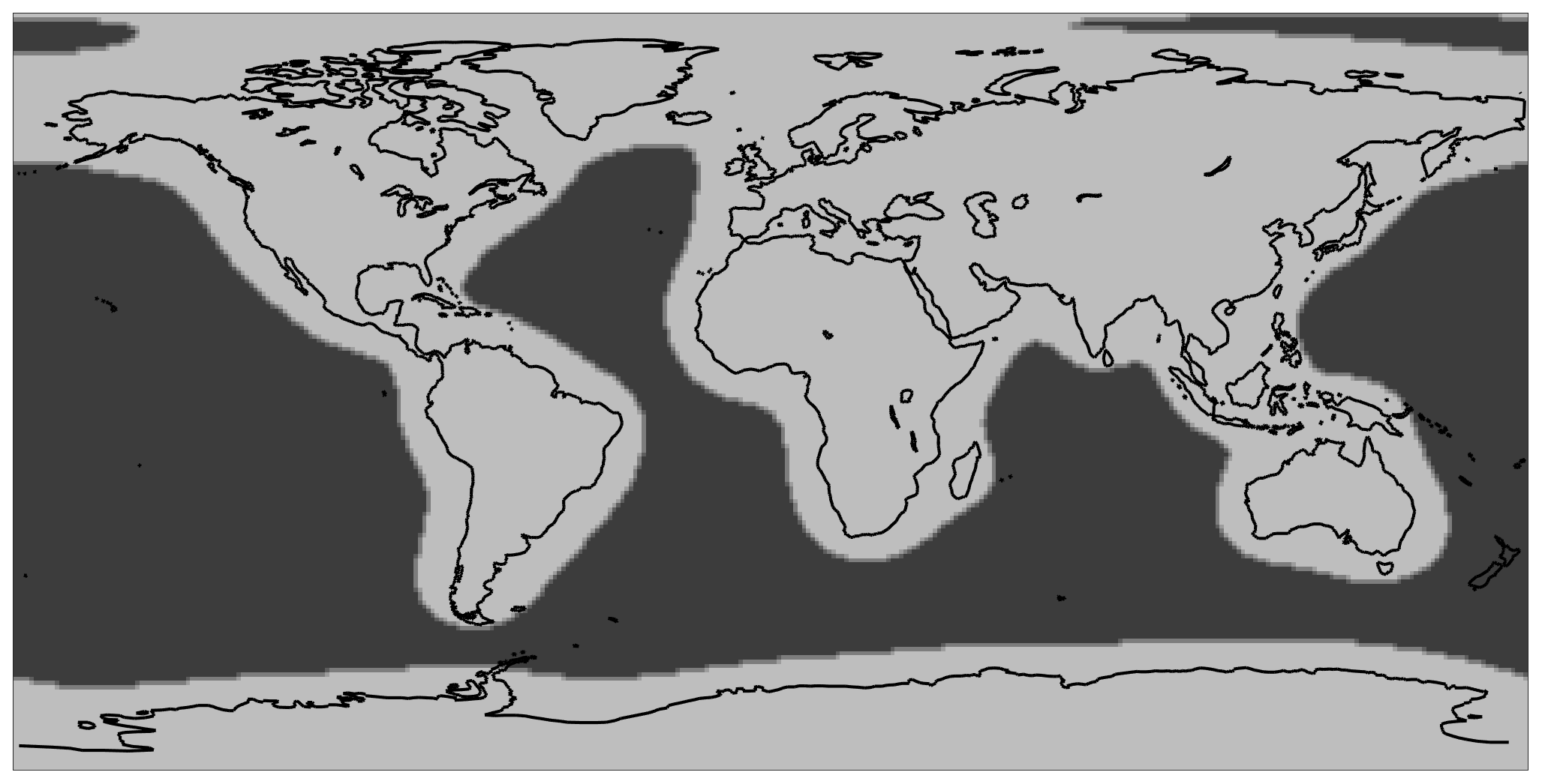
Figure 1 Deep-ocean mask shown as dark areas.

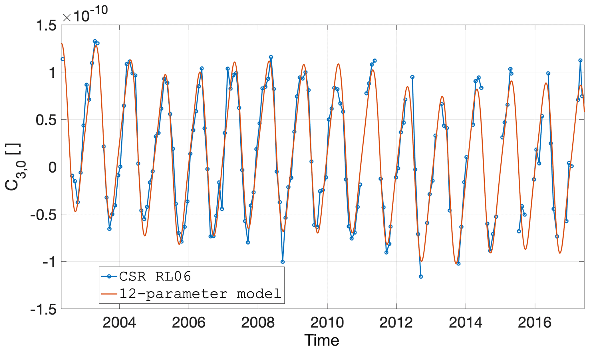
Figure 2 Agreement between the GRACE climatological model and the GRACE data, exemplified by the C_3,0 coefficient.

We selected the first-order polynomial to represent bias and trend in the GRACE data. For the periodic parameters, we choose the year and semi-year periods since these are dominant signals in the GRACE and Swarm data. We also modelled the S2, K2, and K1 tidal periods, with durations of 0.44, 3.83, and 7.67 years, respectively. These periods are driven by the orbital inclination of the GRACE satellites and produce strong aliasing in the GFM time series (Ray and Luthcke, 2006; Cheng and Ries, 2017). The linear regression of the 12 parameters is done independently for each SH coefficient, up to degree 40 (in agreement with the maximum degree of the Swarm models). This results in 12 sets of Stokes coefficients, one for each of the model parameters: bias, trend, and five periods represented by their sine and co-sine components. Each set of parametric Stokes coefficients has an implicit time dependence which is evaluated coefficient-wise at the epochs of the Swarm GFMs. We illustrate the general agreement between the climatological model and the GRACE data for the case of C_3,0 in Fig. 2.

We regard this model as a good representation of the Earth system; it is by definition inferior to the original GRACE time series because it truncates the signal bandwidth to discrete frequencies. In spite of this, the assumed climatological model provides a measure to which both GRACE and Swarm can be compared. The differences between GRACE and this model should be regarded as the signal augmentation that GRACE brings, not as an error. We also regard the vastly different spatial sensitivity of Swarm compared to GRACE as an additional argument that the climatological model is able to represent the Earth system in a much more accurate way than Swarm, with the exception of large atypical mass variations (which are uniquely revealed by Swarm).

3 Results

Our results are shown in the following section, where we analyse the added value of KBs in Sect. 3.1, look into the effect of including accelerometer measurements of Swarm C in Sect. 3.2, provide an overview of the quality of our individual solutions in Sect. 3.3, quantify the quality of the combined solutions in Sect. 3.4, and illustrate their signal content in Sect. 3.5.

3.1 Kinematic baselines

This section is dedicated to quantifying the benefit of exploiting KBs in the quality of the GFMs derived from Swarm data, following the motivation and procedures described in Sect. 2.2.

Due to the decreasing ionospheric activity and the changes made to the Swarm on-board GPS receivers between 2015 and 2016 (van den IJssel et al., 2016), the consistency of the KB solutions has improved. Especially in summer 2016, the overall daily SD of the difference between the reduced dynamic ambiguity-fixed and kinematic ambiguity-fixed baselines may be as low as 10–15, 4–6, and 3–5 mm on average for the radial, along-track, and cross-track directions, respectively, while it is as high as 1–3 cm for 2015 in all three directions. It should be noted, however, that daily SD is always dominated by the low-quality kinematic positions over the polar regions. Eliminating such problematic data, the difference SD is consistently under 5 mm; therefore, the internal precision of the Swarm GPS data is of very good quality.

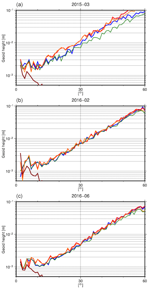
Figure 3 Difference SH degree amplitudes of all four test solutions with respect to GOCO05S, for March 2015 (a), February 2016 (b), and June 2016 (c), regarded as representative of bad, intermediate, and good data quality, respectively.

Table 5 Rms of geoid height differences in millimetres for different hl-SST-only results and the ll-SST and hl-SST Swarm solutions with respect to the corresponding ITSG-Grace2016 monthly solution.

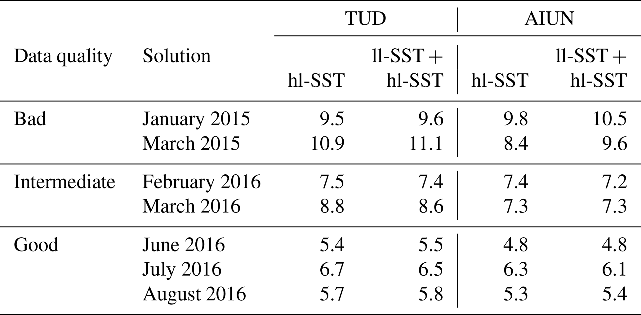
Figure 3 shows the degree amplitudes with respect to the static part of the GOCO release 05 satellite-only gravity field model (GOCO05S) (Mayer-Gürr, 2015) in terms of geoid heights, representative of the results for bad, intermediate, and good data quality. For comparison the corresponding month from the ITSG GRACE-only model 2016 (ITSG-Grace2016) time series is also shown. For all months it can be seen that the solutions do not differ significantly. There are small differences between the two ACs (AIUB and TUD) as well as between the hl-SST-only and the ll-SST + hl-SST solutions. Differences are larger for those months with bad data quality (2015) and at the SH degree regions dominated by noise (above degree 15), with the ll-SST and hl-SST solutions showing larger degree amplitudes. For months with good data quality (June 2016) all four solutions display much smaller differences.

To quantify the impact on the long-wavelength part of the solutions, we have compared the individual solutions to ITSG-Grace2016 monthly solutions in the spatial domain. The solutions are evaluated on an equiangular grid ($\mathrm{1}{}^{\circ }\times \mathrm{1}{}^{\circ }$), reduced by the corresponding ITSG-Grace2016 monthly solution, and filtered with a 500 km Gaussian filter, and finally the rms over all grid cells is computed. The filter width was selected so as to avoid suppressing all of the signal at degrees above 20 in order to assess the impact of KBs on the high-frequency noise as well. These results are summarized in Table 5.

Table 5 confirms what is depicted in Fig. 3; i.e. the inclusion of KBs in the gravity field estimation has no significant impact on the quality of the resulting GFM. KO-only solutions are already of very similar quality when compared to KB-augmented solutions, with small differences visible in the degree amplitude plots or the spatial rms having no discernible correlation with the data period (and therefore quality). In general, this confirms the findings of Jäggi et al. (2009), in that there are some small benefits for higher degrees when using KB; this was attributed to the elimination of errors common to both satellites by using DD observations. Our results suggest that common errors are already mostly absent in the computation of the Swarm KOs. Thus we found no added value in including KBs for the quality of Swarm GFMs.

Our results contrast with those of Guo and Zhao (2019), who demonstrated a noticeable improvement when KBs are used in conjunction with KOs to derive GFMs from hl-SST GRACE data. As the authors mention, their approach benefits from the 3D KB information, thus essentially increasing by a factor of 3 the number of observations. Although these components are most likely not completely independent, they provide observations with crucial information that is not available along the line-of-sight (LoS) component, in particular along the radial direction. We also note that the geometry of the GRACE formation provides a much more stable amplitude and attitude of resulting KBs, which may benefit the ambiguity fixing and, consequently, their overall quality. In the case of Swarm, the KBs are close to zero and flip their orientation by 180^∘ at the poles. Additionally, GRACE accelerometer data were used to represent the non-gravitational accelerations, which is less straightforward for the Swarm satellites. These differences, i.e. 3D baselines, stable baseline length, and inclusion of accelerometer data, suggest that they may be necessary conditions for a positive added value of KBs to the quality of hl-SST-only GFMs. Finally, we also point out that the improvements reported in Guo and Zhao (2019) are only above SH degree 10, where the errors start to become dominant, thus reducing the practical added value of including baselines in the estimation of hl-SST-only GFMs.

3.2 Non-gravitational accelerations

In this section, we present the inter-comparison of the three types of non-gravitational accelerations described in Sect. 2.3. Figure 4 compares three single-satellite gravity field solutions derived from Swarm C data, considering the three non-gravitational accelerations, for January 2015.

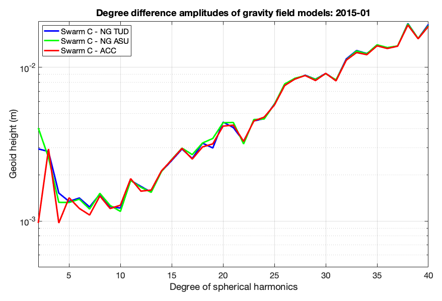
Figure 4 Swarm C gravity field solutions using TUD and ASU modelled non-gravitational accelerations, as well as measured nongravitational accelerations (January 2015).

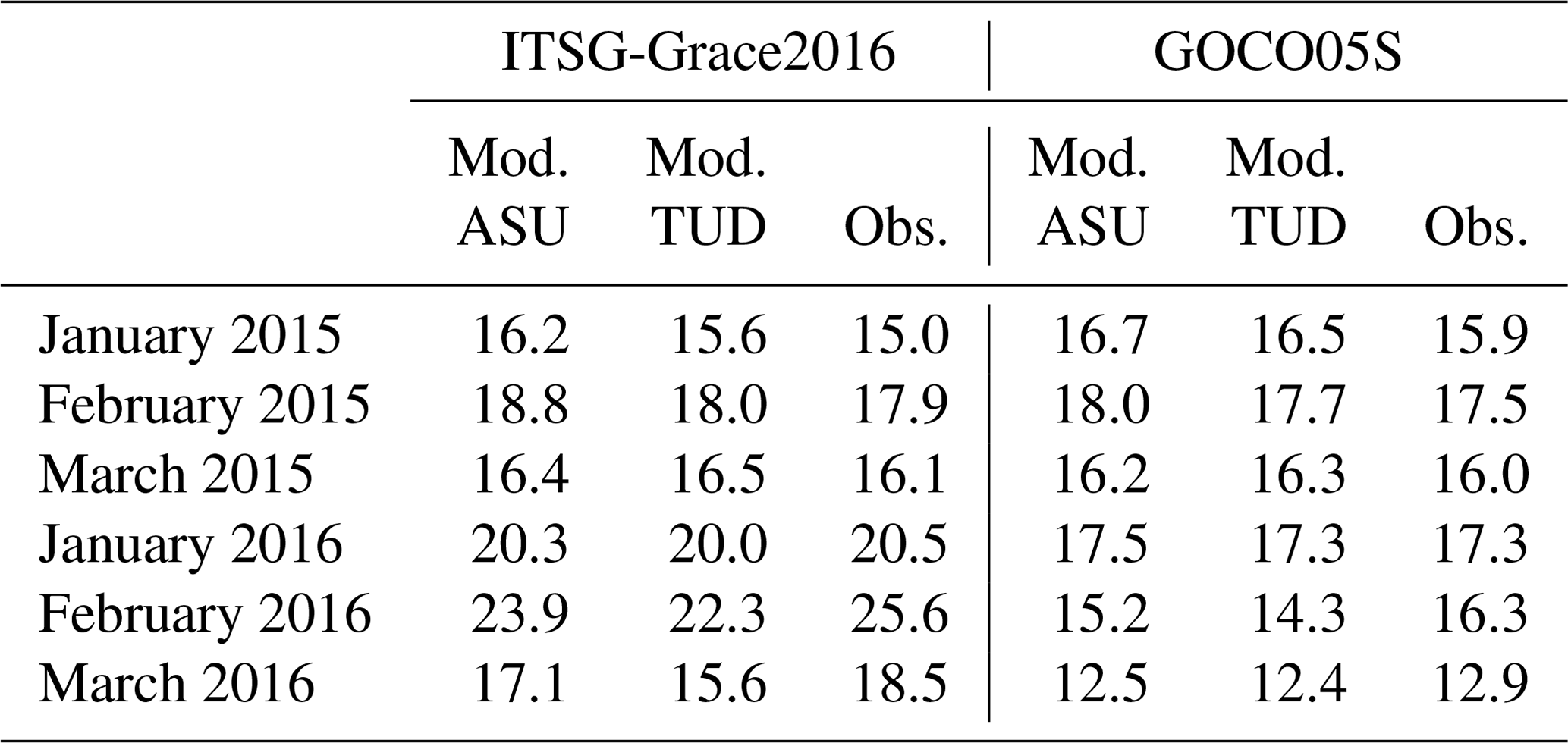
The SH degree difference amplitudes illustrate that the measured non-gravitational accelerations improve the agreement of the lowest degrees of the Swarm C monthly solution with respect to the GOCO05S model (Mayer-Gürr, 2015), which includes a time-variable component. We tested this comparison relative to the ITSG-Grace2016 monthly GFM (Mayer-Gürr et al., 2016) and observed similar results (not shown). The improvement at the lowest degrees in the Swarm C model when using observed non-gravitational acceleration data is in accordance with what was reported by Klinger and Mayer-Gürr (2016), relative to GRACE gravity field recovery.

In view of the lack of reliable measured non-gravitational accelerations in Swarm A and Swarm B, the three-satellite Swarm GFM considers the ASU modelled non-gravitational accelerations for these satellites. For Swarm C, we consider three cases where the non-gravitational accelerations are either measured or represented by TUD or ASU's model. In this way, we isolate the effect of the three types of non-gravitational acceleration data. The results for January 2015 are shown in Fig. 5, using ASU and TUD models and calibrated accelerometer data.

Table 6 Geoid height difference in millimetres between Swarm and GRACE GFMs.

The three-satellite solutions that use modelled non-gravitational accelerations in Swarm C are remarkably similar (see Fig. 5). In spite of this, note that using accelerometer data improved the agreement to GOCO05S for degrees 2 and 4.

To gather a better overview of the added value of the three types of non-gravitational accelerations, we derive the following model difference D, similar to rms:

$$\begin{array}{}\text{(1)}& D=\sqrt{\mathrm{median}{\left(\mathrm{\Delta }h\right)}^{\mathrm{2}}+\mathrm{MAD}{\left(\left|\mathrm{\Delta }h\right|\right)}^{\mathrm{2}}},\end{array}$$

with the median absolute deviation (MAD) analogous to SD when the median is considered instead of the mean and Δh being the $\mathrm{1}{}^{\circ }\times \mathrm{1}{}^{\circ }$ geoid height difference between the 500 km Gaussian filtering three-satellite Swarm models and both ITSG-Grace2016 and GOCO05S, in the latitude band 85^∘ from the Equator. We note that similar results were obtained using the CSR RL05 GRACE monthly solutions (not shown). The resulting differences are shown in Table 6.

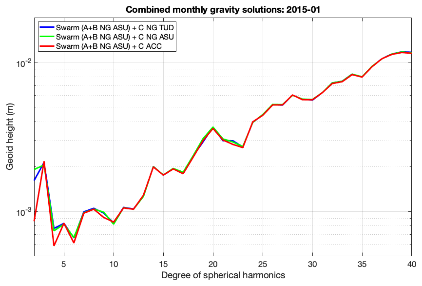
Figure 5 Three-satellite Swarm gravity field solutions using TUD- and ASU-modelled non-gravitational accelerations, as well as measured non-gravitational accelerations for Swarm C and ASU-modelled non-gravitational accelerations for Swarm A and B (January 2015).

The 2015 results indicate that the observed non-gravitational accelerations improve the agreement between the three-satellite Swarm models and ITSG-Grace2016 and GOCO05S, while that is not the case for 2016 (except for January 2016 and GOCO05S, when the GFM derived from TUD-modelled non-gravitational accelerations agrees equally well with the one derived considering observed non-gravitational accelerations). The comparison with GOCO05S intends to predict how possible it would be to assess the added value of the different types of non-gravitational accelerations during those periods when there are no GRACE data. Other time-dependent models were tested, but those do not agree as closely with GRACE monthly models (not shown).

The statistics in Table 6 imply that observed non-gravitational accelerations are only beneficial when the amplitude of the non-gravitational accelerations is larger than what was observed in 2016. This is likely related to the decreasing level of solar activity, which is approaching the minimum of its 11-year cycle (expected to reach the minimum in 2019). Through the influence of the solar radiation on the atmospheric density and resulting atmospheric drag, the low level of solar activity has a direct impact on the accelerometer measurements. The closer to the solar cycle minimum, the lower magnitude and variability of the accelerometer signal are. Another factor may be a potential worse performance of the accelerometer calibration procedure under low levels of solar activity, resulting from the lower signal-to-noise ratio (SNR) in the accelerometer data. In other words, the noise and (potentially) uncorrected artefacts in the accelerometer data of Swarm C are substantial enough to limit the usefulness of these data to gravimetric studies, except when the solar activity is high (as was the case in 2015) or when the satellites' altitude decays in the future. Given these characteristics and the continuing solar minimum, our Swarm models are not processed considering Swarm C accelerometer observations, but we plan to revisit this issue once the solar activity increases.

3.3 Individual Swarm models

In this section we illustrate the quality of the individual Swarm solutions. As described in Sect. 2.6, we directly compare Swarm at the epochs defined by GRACE under 750 km radius Gaussian smoothing.

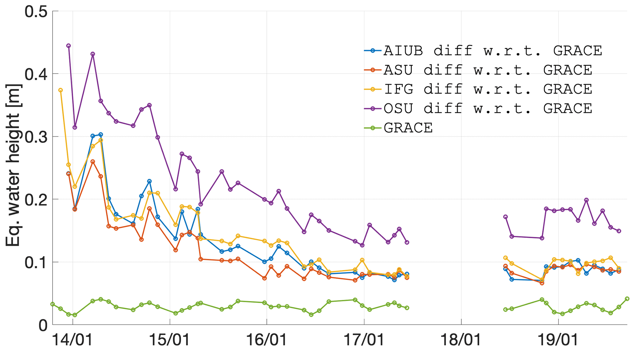
Figure 6 Time dependence between December 2013 and September 2019 of the epoch-wise cumulative degree amplitude (or global spatial rms) of the individual Swarm solutions, CSR RL06 GRACE, and their difference, considering 750 km smoothing.

Figure 6 shows a measure of the evolution of the quality of the individual Swarm solutions over the complete Swarm data period. We also plot the cumulative degree amplitude of GRACE, to illustrate the global spatial amplitude of the geophysical processes represented by these data. There is a clear improvement in the agreement of Swarm with GRACE, from rms differences as high as 40 cm geoid height in early 2014, down to 10 cm and below since 2016. We attribute this increase in quality to the decrease in solar activity and to the upgrades in the Swarm GPS receivers between 2015 and 2016 (van den IJssel et al., 2016; Dahle et al., 2017). As demonstrated in Sect. 3.4, the Swarm models contain large errors in the ocean areas, which dominate the global spatial rms difference; over land areas, the agreement with GRACE is much better.

The various individual solutions show different levels of quality. Generally speaking, the solutions from AIUB, ASU, and IfG cluster together as agreeing better with GRACE, with their dispersion narrowing down after 2016. This suggests that these approaches suffer differently in conditions of high solar activity, with ASU's models being the least sensitive overall. Possibly, ASU's efforts to minimize the amplification of the high frequencies when performing the double differentiation of the kinematic positions has the side effect of suppressing the negative effects of the high solar activity in the quality of the kinematic orbits. In contrast, OSU's solution consistently has lower agreement with GRACE. The velocity measurements, which are needed for IEBA (as well as any EBA-type approach), are to be derived from the kinematic positions by differentiation (then squared to obtain kinetic energy). The tedious data filtering and processing to approximate velocity errors is still imperfect, particularly in light of the spurious jumps in most of the kinematic orbits even in the cases without the GPS tracking signal degradation, e.g. from the southern Atlantic anomaly.

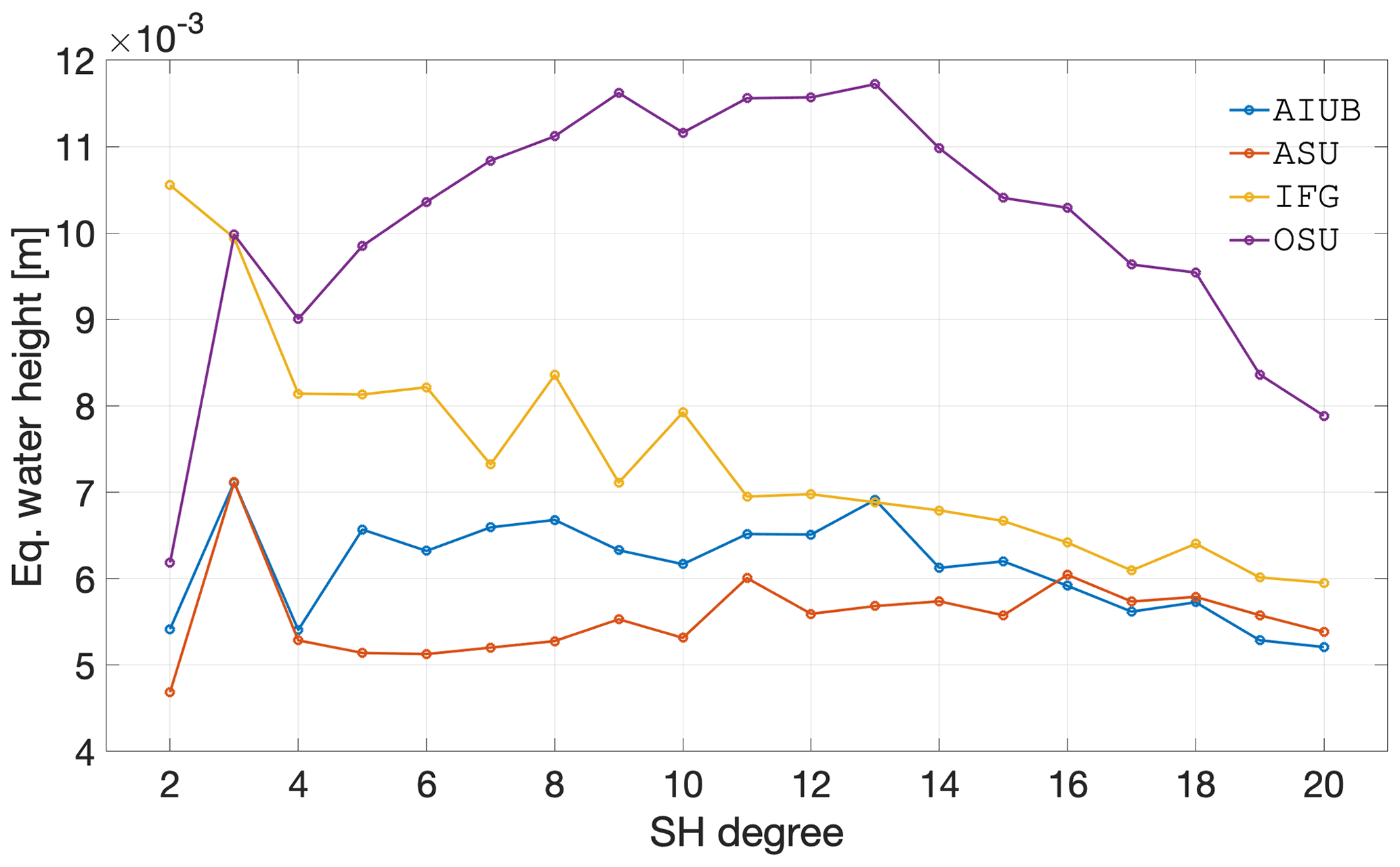
Figure 7 Spectral agreement over the period between December 2013 and September 2019 in terms of the degree mean of the per-coefficient temporal rms difference, of the individual Swarm solutions, CSR RL06 GRACE, and their difference, considering 750 km smoothing.

Another way of analysing the agreement between the individual solutions and GRACE is to derive per-coefficient statistics of their temporal variations. One such statistic is the coefficient-wise temporal rms of the difference between the Swarm individual solutions and GRACE, thus producing a set of Stokes coefficients that describes the variability of that difference; from this set we compute the mean over each degree to represent the general agreement at the corresponding spatial wavelengths. The results are summarized in Fig. 7, which quantifies the agreement of Swarm and the GRACE climatological model in the spectral domain. Note that for most individual solutions, the rms difference decreases with degree as a result of the Gaussian smoothing, without which the curves would have a strong overall positive slope.

The ranking of quality of the individual solutions changes with spatial wavelength; for example, although OSU's solutions are consistently worse than IfG's as shown in Fig. 6, their degrees 2 and 3 are on average in equal or better agreement with GRACE. This diversity in the particularities of the various solutions is the main motivation for our practice to combine solutions derived from multiple gravity field estimation approaches. Unfortunately, as explained in Sect. 2.5, our combination is done at the solution level with weights derived from VCE, which means we loose the ability to weight the individual solutions differently in the degree domain and we cannot fully take advantage of the per-degree variations in quality of the individual solutions. Nevertheless, the VCE weights produce combined solutions with better agreement with GRACE than those combined at the NEQ level (Teixeira da Encarnação and Visser, 2019). From this we interpret that the benefits from per-degree weighting may not be as significant as the disadvantages of the combination at NEQ level, namely the different types of formal and calibrated errors, their different temporal evolution, and the difficulty in finding adequate empirical weights.

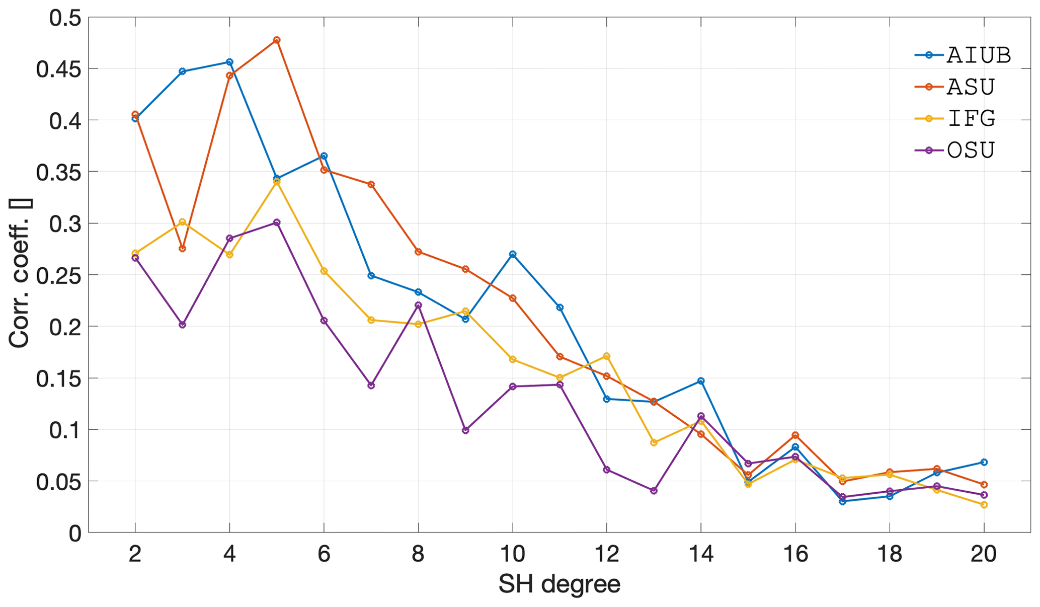
Figure 8 Spectral correlation over the period between December 2013 and September 2019 in terms of the degree mean of the per-coefficient temporal correlation coefficient, of the individual Swarm solutions, CSR RL06 GRACE, and their difference, considering 750 km smoothing.

Finally, Fig. 8 shows the correlation of the Swarm time series with GRACE for the relevant spatial wavelengths. This figure is complementary to Fig. 7, since it does not illustrate the overall agreement (which is a measure of error) but the level that Swarm observes the same temporal evolution as GRACE (i.e. if Swarm sees the same proportional mass increase or decrease as GRACE). Understandably, the highest correlations correspond to the lowest degrees, not only because those are the signals with the highest amplitude (and therefore better observed by Swarm and GRACE) but also because of the smoothing. There is no obvious individual solution that stands out as being better correlated with GRACE, although ASU has the highest correlation coefficient for degrees 2, 4, and 7 to 9, while for AIUB that is the case for degrees 3 and 4. OSU's solution tends to correlate the least, except for degrees 4 and 8; this again indicates that a solution that may at first seem to be of consistently inferior quality may still provide a positive contribution to the combination. Also note that the correlations drop below 0.1 above degree 14 and remain relatively constant for higher degrees, indicating there is very little signal in the individual solutions that represent the same temporal variations as GRACE.

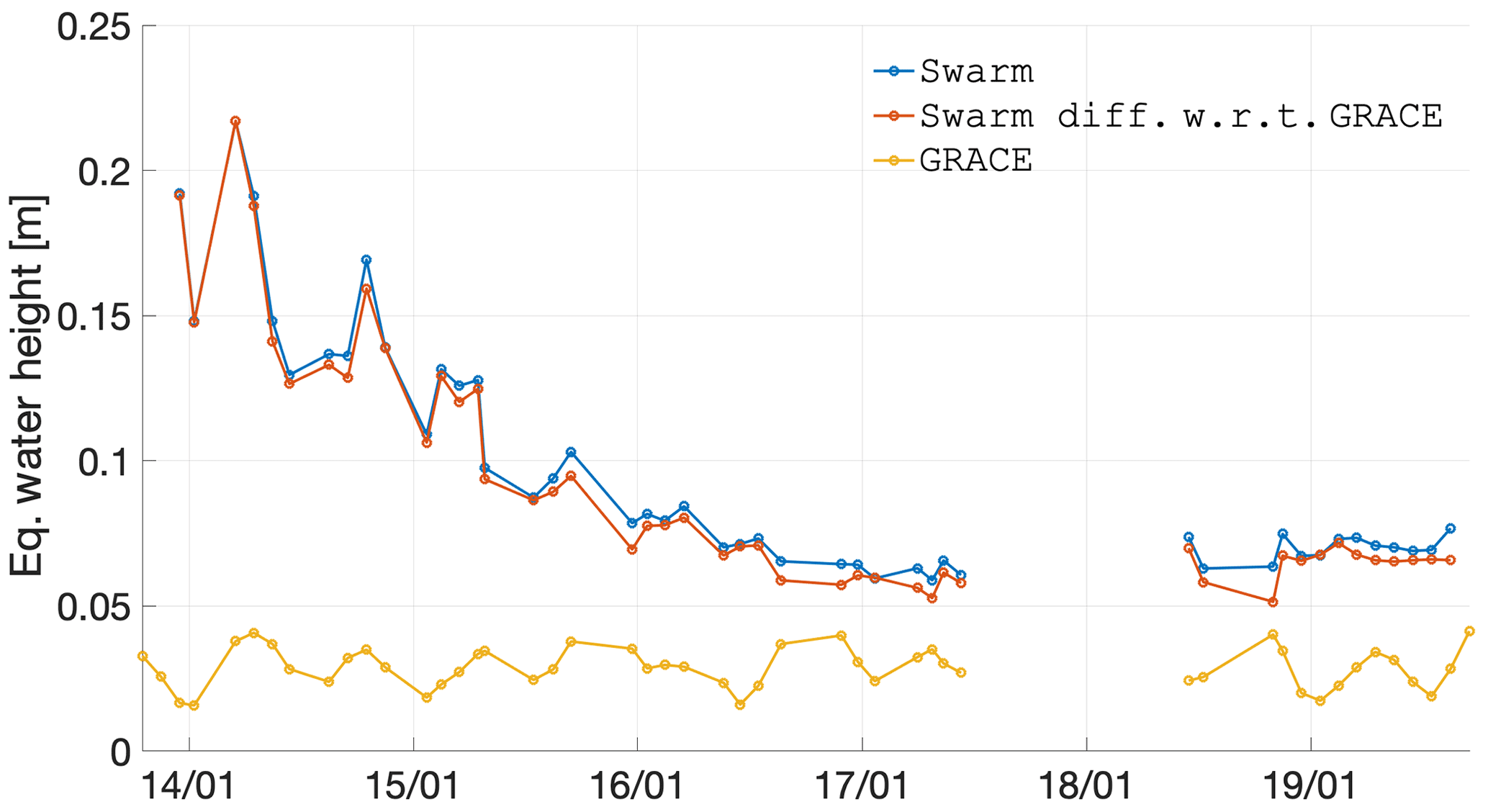
Figure 9 Time dependence between December 2013 and September 2019 of the epoch-wise cumulative degree amplitude (or global spatial rms) of the combined Swarm solutions, CSR RL06 GRACE, and their difference, considering 750 km Gaussian smoothing.

3.4 Combined Swarm models

Having presented the individual Swarm GFMs in the previous section, we dedicate the current section to the analysis of the combined solutions. For more details about the combination strategy, refer to Teixeira da Encarnação and Visser (2019) and Meyer (2020). We determine the necessary intensity of smoothing of the Swarm models (Sect. 3.4.1) and illustrate the different sensitivity of the Swarm data to observe mass transport processes over land and ocean areas (Sect. 3.4.2).

3.4.1 Smoothing of the Swarm solutions

As demonstrated by Teixeira da Encarnação et al. (2016), the Swarm models do not seem to be sensitive to full wavelengths shorter than roughly 1500 km. We now update this assessment in light of the much longer time series and improved combination strategy than was the case in earlier publications. We compute the cumulative degree amplitude (which is proportional to the global spatial rms) of the difference between the Swarm and GRACE models and the unsmoothed GRACE climatological model, for two levels of smoothing radii: 750 km (Fig. 9) and 1500 km (Fig. 10).

For the 750 km case, the Swarm difference nearly always has the same amplitude as the Swarm signal itself. We will demonstrate in Sect. 3.4.2 that a significant portion of the amplitude of the Swarm difference is located over ocean areas and the agreement over land is significantly better. In spite of this, the lower amplitude of Swarm relative to the GRACE data suggests this smoothing intensity is inadequate to isolate the geophysical signal in the Swarm time series at the global scale.

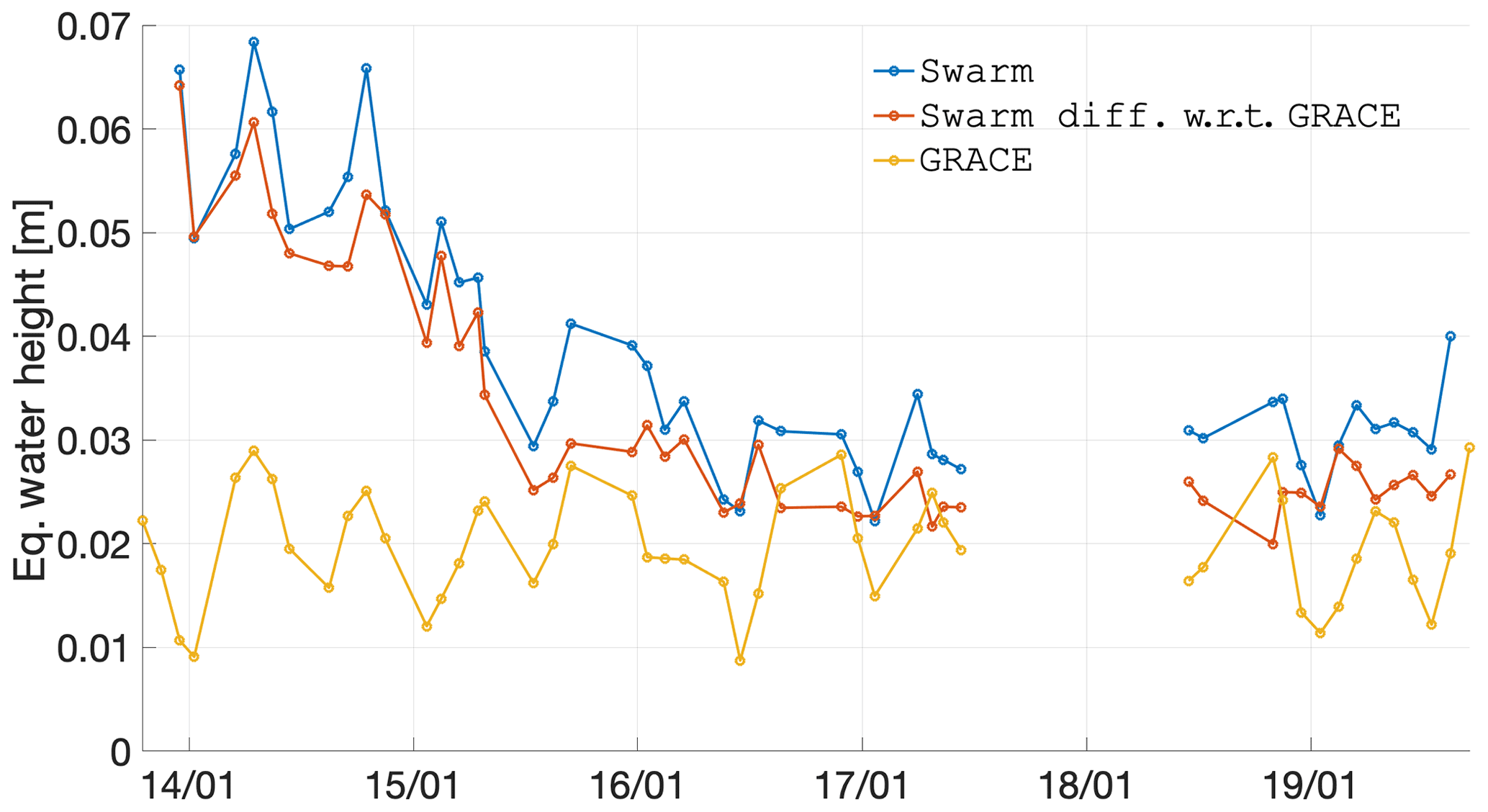
Figure 10 Time dependence between December 2013 and September 2019 of the epoch-wise cumulative degree amplitude (or global spatial rms) of the combined Swarm solutions, CSR RL06 GRACE, and their difference, considering 1500 km Gaussian smoothing.

In the case of 1500 km smoothing, the Swarm differences have comparable amplitudes to the GRACE data since mid-2015. We interpret this observation, given the conservative nature of the Swarm global rms difference, as indication that there is unnecessary suppression of the signal at spatial wavelengths from the two smoothing intensities considered in Figs. 9 and 10 (roughly 1500 to 3000 km, since we report smoothing radii).

We also repeated this exercise for the cases of no smoothing and 300 km smoothing radius. Those results indicated that the errors above degree 12 dominate the solution and produce monthly differences of negligible difference relative to the full Swarm spatial variability (not shown).

3.4.2 Land and deep-ocean signal

This section illustrates the differences in SNR characteristic of the Swarm GFMs by computing separate statistics for land and deep-ocean areas, the latter defined in Sect. 2.6.2.

In Fig. 11 the rms of the deep-ocean areas is shown in terms of the difference between the Swarm and GRACE solutions. As expected, the GRACE GFMs over the oceans have a relatively small amplitude, well under 2 cm EWH. Additionally, the Swarm GFMs show differences which are of much higher amplitude than the ocean signal represented by the GRACE data and barely different than the magnitude of the Swarm signal itself. In other words, Swarm is unable to resolve any monthly ocean signal with the spatial scales that GRACE can observe; however, the same cannot be said about (i) long-term trends since the data were de-trended prior to computing the statistics in Fig. 11 or (ii) aggregate measures such as the global ocean mass reported by Lück et al. (2018).

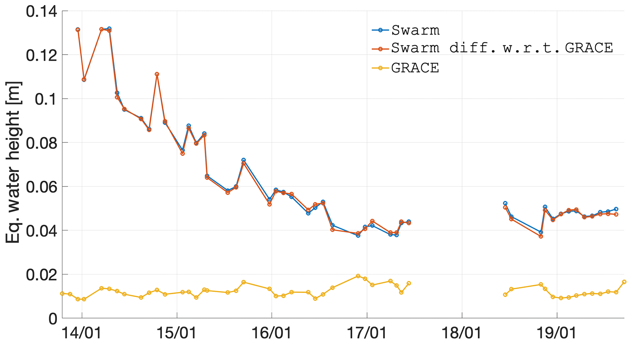
Figure 11 Time dependence between December 2013 and September 2019 of the epoch-wise cumulative degree amplitude (or global spatial rms) of the combined Swarm solutions, CSR RL06 GRACE, and their difference, for deep-ocean areas considering 750 km smoothing.

We illustrate the agreement of Swarm and GRACE solutions in the spectral domain in Fig. 12 (which is produced in a similar way as Fig. 7). Similar to the evolution of the temporal agreement represented in Fig. 11, the spectral analysis illustrates that Swarm differs from the climatological model with amplitudes that surpass the signal, across all the spatial wavelengths, over the oceanic areas. The only exception refers to degree 2 but that is mainly driven by the consistent use of C₂₀ published in Cheng and Ries (2018).

Figure 12 Spectral agreement over the period between December 2013 and September 2019 in terms of the degree mean of the per-coefficient temporal rms difference, of the combined Swarm solutions, CSR RL06 GRACE, and their difference, for deep-ocean areas considering 750 km smoothing.

When it comes to land areas, the Swarm solutions agree with the climatological model much better than in the oceans. Figure 13 shows that since 2016, the Swarm difference with respect to the GRACE data has comparable amplitude. This means that Swarm is generally able to observe the majority of mass transport processes described by the climatological model (under Gaussian smoothing with 750 km radius), in particular after 2016. Prior to mid-2015, this is on average not the case, although we will demonstrate in Sect. 3.5.3 that regions where the mass transport signal is of substantial amplitude are reasonably well observed.

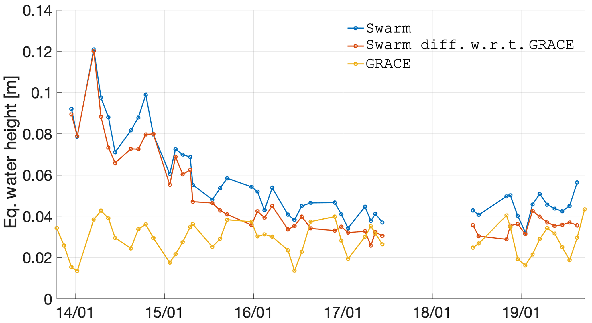
Figure 13 Time dependence between December 2013 and September 2019 of the epoch-wise cumulative degree amplitude (or global spatial rms) of the combined Swarm solutions, CSR RL06 GRACE, and their difference, for land areas considering 750 km smoothing.

The analysis in the spectral domain summarized in Fig. 14 confirms that the difference with respect to the climatological model is of smaller amplitude than the signal therein represented up to degree 12. This result further confirms the result of Sect. 3.4.1 regarding de adequacy of smoothing the Swarm solutions with a Gaussian filter with 750 km radius.

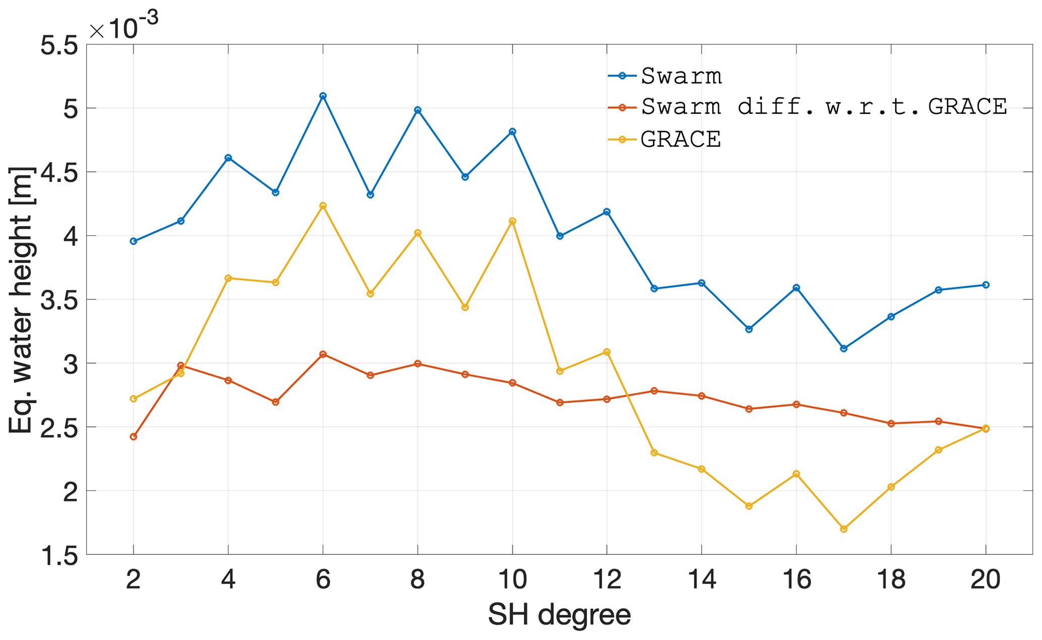
Figure 14 Spectral agreement over the period between December 2013 and September 2019 in terms of the degree mean of the per-coefficient temporal rms difference, of the combined Swarm solutions, CSR RL06 GRACE, and their difference, for land areas considering 750 km smoothing.

The results presented in Figs. 11–14 illustrate that the Swarm GFMs are unable to resolve the gravity signal in the oceanic regions at spatial lengths comparable to land areas. We observe that the discrepancy with respect to GRACE over the ocean is roughly 25 % larger than over land. We do not have a definitive explanation for this, other than the ionospheric activity may corrupt the estimated gravity field parameters over the oceans more significantly since away from land areas there is very little gravity signal to capture. In other words, the natural gravity variations over land are of sufficient amplitude to dominate the errors, at least enough to drive our statistics.

The higher accuracy over land could be explained by the ionospheric activity affecting mainly ocean areas, since those are mostly located along the Equator (e.g. the Pacific ocean). Masking the land areas could therefore remove the large land signals associated with hydrology and leave mostly the errors in the equatorial oceans. To test this hypothesis, we masked the Swarm and GRACE residual along tropical and non-tropical regions, as illustrated in Fig. 15.

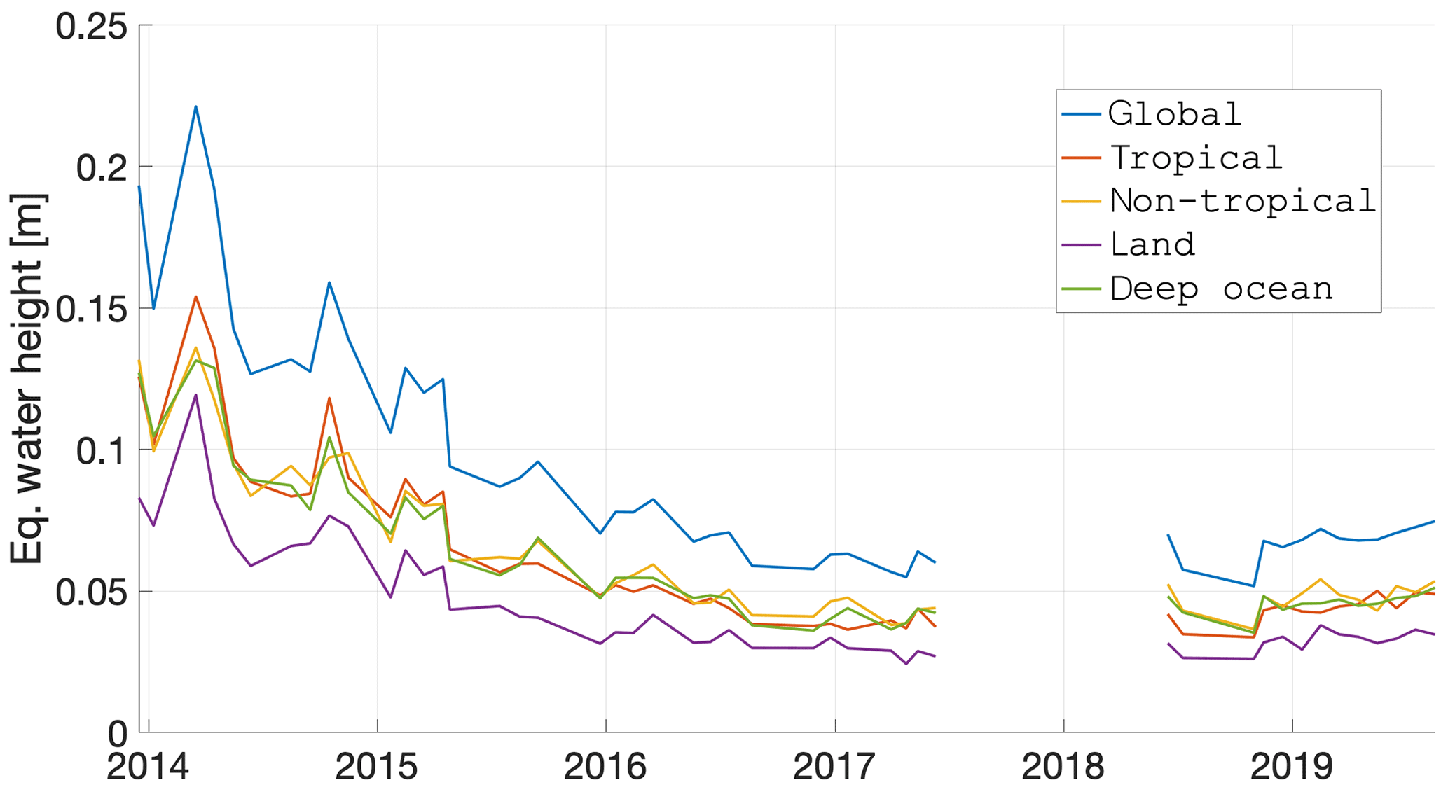
Figure 15 Time dependence between December 2013 and September 2019 of the epoch-wise cumulative degree amplitude (or global spatial rms) of the combined Swarm solutions masked over different regions, considering 750 km Gaussian smoothing.

It is clear that Swarm observes the tropical regions, which include regions with strong gravitational variations such as the Amazon basin and vast ocean areas in the Pacific, in as good agreement as the non-tropical regions. We note that the deep-ocean regions are not complementary of the land regions (i.e. the two domains do not cover the whole Earth; see Sect. 2.6.2) and it should not be expected that their spatial rms is proportionally larger than the tropical and non-tropical regions, which are of comparable amplitude between themselves and complementary.

We now focus on the necessary smoothing to retrieve any deep-ocean signal from the monthly Swarm models. We increased the smoothing intensity relative to what is discussed in Sect. 3.4.2 to demonstrate the capabilities of Swarm to contribute to ocean studies, in particular those related to large-scale mean dynamic ocean topography. For the case of global ocean mass Lück et al. (2018) already demonstrated an agreement with GRACE of less than 5 mm in terms of EWH. We tested smoothing radii of 1000, 1500, 3000, and 5000 km; the results for 3000 km are presented in Figs. 16 and 17.

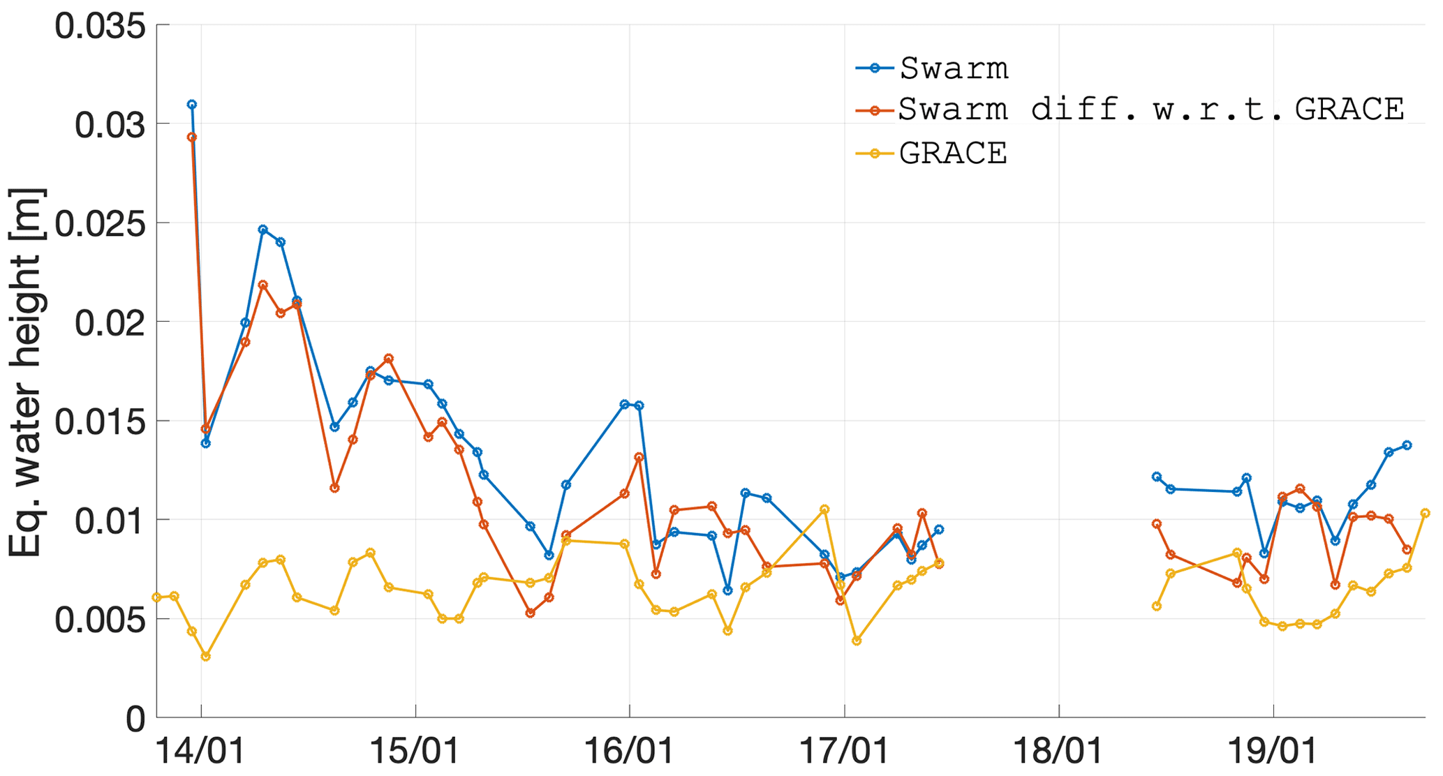
Figure 16 Time dependence between December 2013 and September 2019 of the epoch-wise cumulative degree amplitude (or global spatial rms) of the combined Swarm solutions, CSR RL06 GRACE, and their difference, for deep-ocean areas considering 3000 km smoothing.

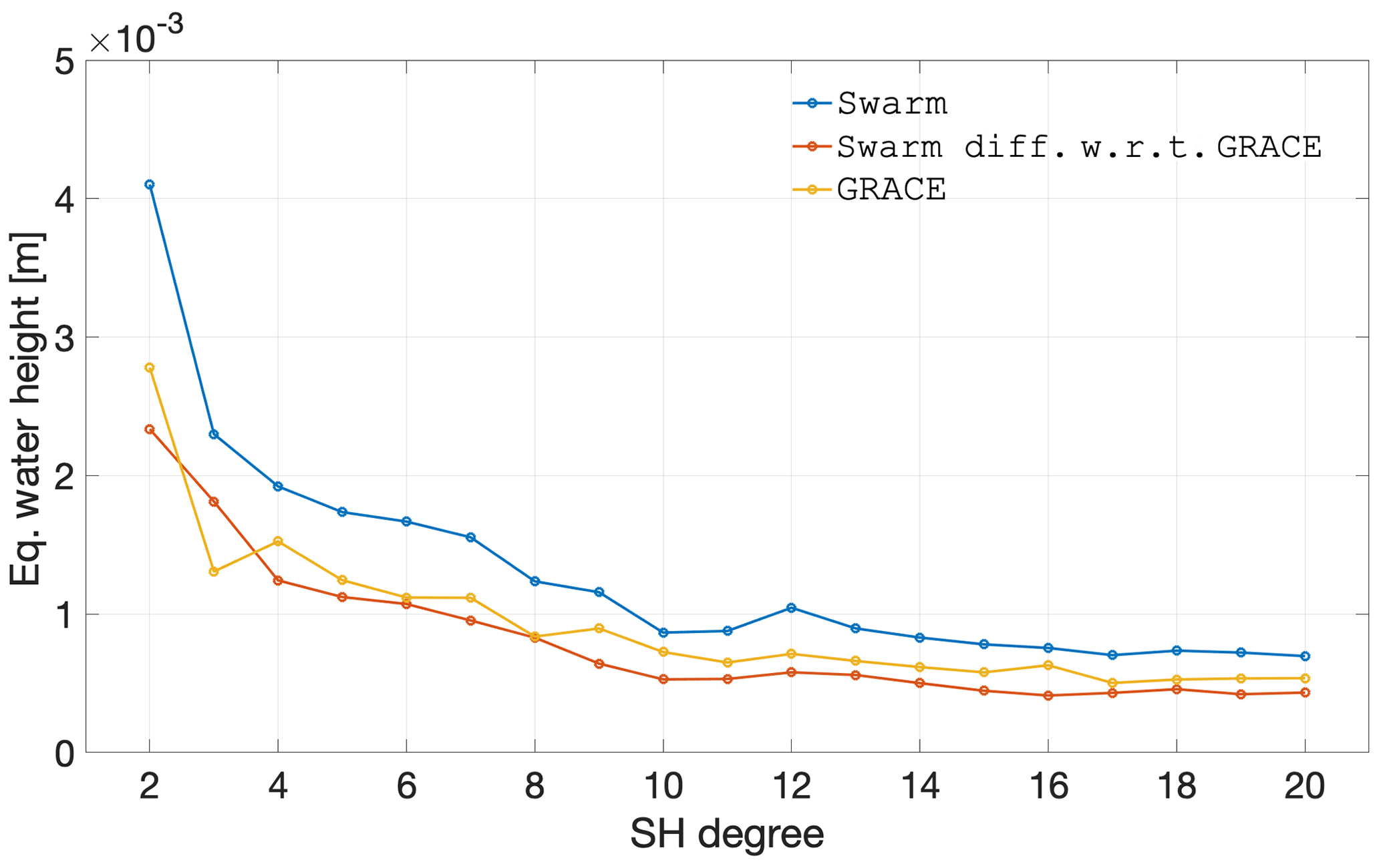
Figure 17 Spectral agreement over the period between December 2013 and September 2019 in terms of the degree mean of the per-coefficient temporal rms difference, of the combined Swarm solutions, CSR RL06 GRACE, and their difference, for deep-ocean areas considering 3000 km smoothing.

Figure 16 demonstrates that a smoothing radius of 3000 km is enough to reduce the spatial rms of the Swarm residual to amplitudes comparable to the signal in GRACE, particularly after 2016. This means that since 2016 Swarm has been observing ocean mass changes at the extremely coarse spatial scale of roughly 6000 km.

We further demonstrate Swarm's ability to resolve large-scale ocean mass changes in the spectral domain, Fig. 17. As illustrated, the smoothing radius of 3000 km is barely enough to, on average, decrease the degree average of the per-degree rms difference below the GRACE signal amplitude. Note that the spectral measure represented by the degree average considered the complete Swarm period, including the start of the mission, when the quality of the solutions was the lowest. Therefore, the smoothing radius of 3000 km is adequate to resolve large-scale Swarm deep-ocean mass changes since mid-2015.

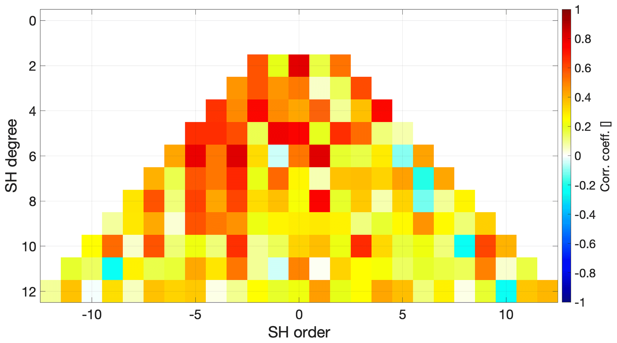
Figure 18 Per-coefficient correlation coefficient between the GRACE climatological model and Swarm.

3.5 Signal content

This section describes the geophysical signal represented by the Swarm models. We start by illustrating the time series of a few low-degree coefficients in Sect. 3.5.1. The variability of the Swarm model, and the patterns therein, is discussed in Sect. 3.5.2. We end with Sect. 3.5.3, where we give an overview of the capabilities of the Swarm models to observe large basin storage variations and how they compare to GRACE and GRACE-FO.

3.5.1 Low degrees

We now present the time series of a selection of low degree coefficients, without any smoothing applied. This section aims at illustrating the noise characteristics of the Swarm models in the time domain and how they compare to GRACE.

We give an overview of the per-degree correlation coefficients of Swarm and GRACE relative to the climatological model. The degree 2 coefficients (except C_2,0), which are particularly important for sea-level studies, are subsequently presented. Finally, we show the selected case of $C_{\mathrm{5},-\mathrm{1}}$ that has an interesting temporal evolution and how Swarm and GRACE capture those signals. The time series of the zonal coefficients from degrees 3 to 5 are presented in Appendix D. Note that we represent the sine Stokes coefficients with negative order, e.g. $C_{\mathrm{2},-\mathrm{1}}$.

Figures 18 and 19 represent the correlation coefficient of the time series of Swarm and GRACE relative to the climatological model, including the early period of the mission when the quality of the Swarm models was lower. As expected, GRACE's coefficients correlated much more closely to the climatological model, as represented by the numerous dark red pixels in the triangular plot of Fig. 19. The overview of Swarm's correlation with the climatological model (Fig. 18) is dominated by values of around 0.2 (represented by a yellow colour), with some regions with average correlations of roughly 0.6 (represented by the red colour), notably for orders −5 to −3 and degrees 9 to 4. Furthermore, we observe some interesting common features in both Swarm and GRACE correlation plots, namely order −6 and C_5,5 seem to be poorly captured by the climatological mode, since neither Swarm nor GRACE correlated well.

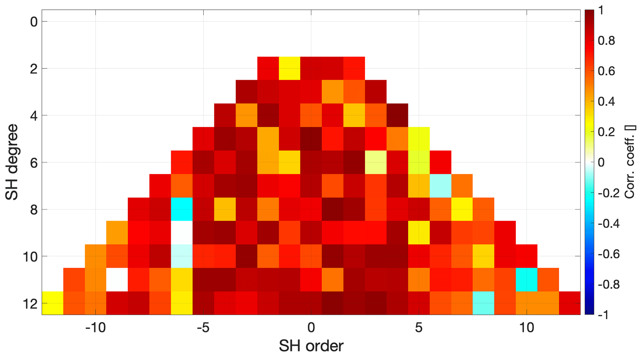
Figure 19 Per-coefficient correlation coefficient between the GRACE climatological model and GRACE.

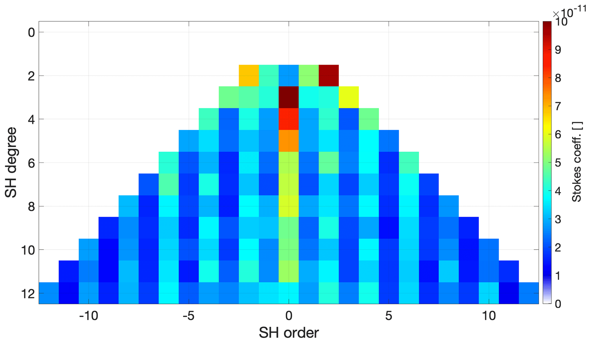
Figure 20 Per-coefficient rms of the difference between the GRACE climatological model and Swarm.

Figure 20 illustrates one particularity of the Swarm models. The rms of the difference relative to the GRACE climatological model is heavily order dependent, with the even orders showing a larger rms than the odd orders (for degrees 4 and above); this effect is particularly striking for orders 6 and −6, as well as for 5 and −5. This feature is also present in the individual models (not shown), in spite of the fact that no order dependency is present in their formal errors. We cannot find an explanation for the discrepancy between the rms difference in even and odd orders.

Figures 21–24 show the time series of the degree 2 coefficients. They illustrate the general characteristics of Swarm coefficient time series: large signal amplitudes, in particular before mid-2015, as well as a general agreement in the average value, if one could imagine a heavy temporal smoothing operation. The last characteristic, which is extremely common for all the coefficients we have analysed (up to degree 6, not all shown here), finds a rare exception in C_2,1, particularly before 2017. A possible explanation is related to the mean pole model (Wahr et al., 2015), which differs between our Swarm solutions (Appendix C) and CSR RL06 (Bettadpur, 2018).

Figure 21 Coefficient C_2,2 as observed by GRACE and Swarm, as well as represented by the GRACE climatological model.

Figure 22 Coefficient C_2,1 as observed by GRACE and Swarm, as well as represented by the GRACE climatological model.

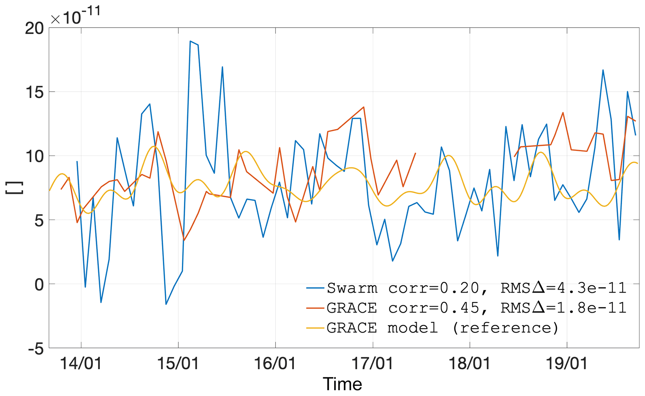
Figure 23 Coefficient $C_{\mathrm{2},-\mathrm{1}}$ as observed by GRACE and Swarm, as well as represented by the GRACE climatological model.

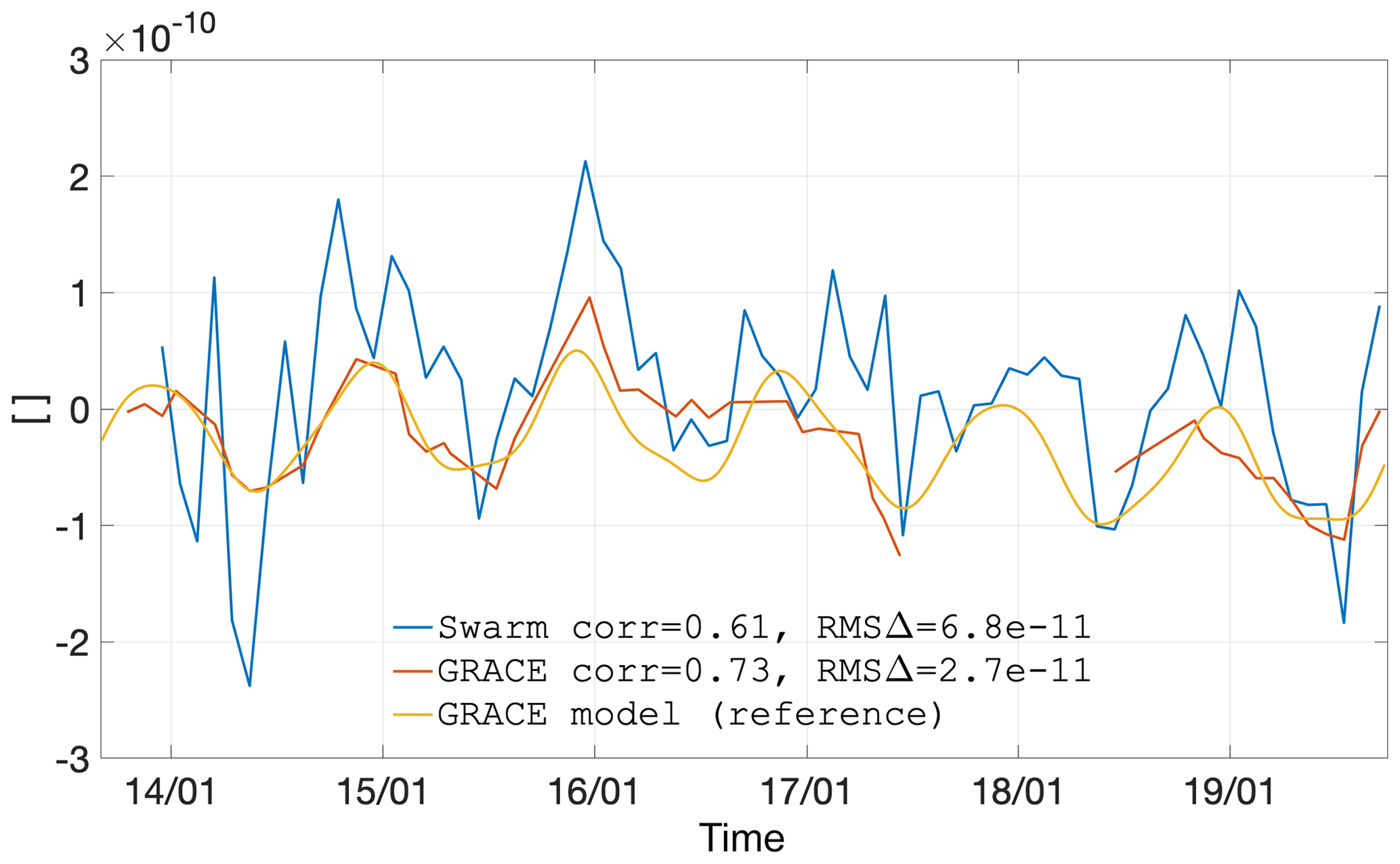
Figure 24 Coefficient $C_{\mathrm{2},-\mathrm{2}}$ as observed by GRACE and Swarm, as well as represented by the GRACE climatological model.

Regarding the agreement of the temporal signal captured by Swarm and that captured by GRACE, it is generally possible to observe that Swarm tends to follow roughly in the same direction, albeit with large month-to-month changes (i.e. larger errors) and with frequent over-shootings before 2016. The large errors are the result of the Swarm solutions exploiting the less accurate kinematic positions as gravimetric observations (in comparison to the much more accurate inter-satellite ranges (ISRs) of GRACE). The errors tend to be larger before 2016, during the period of higher solar and ionospheric activity as well as prior to the GPS receiver tracking loop updates (van den IJssel et al., 2016; Dahle et al., 2017).

Figure 25 shows a representative case of a good agreement between Swarm and GRACE. The overall trend of the $C_{\mathrm{5},-\mathrm{1}}$ coefficient is well represented in the climatological model but fails to capture the abnormal deviation around early 2016, which is observed in a consistent way by GRACE and Swarm.

Figure 25 Coefficient $C_{\mathrm{5},-\mathrm{1}}$ as observed by GRACE and Swarm, as well as represented by the GRACE climatological model.

3.5.2 Signal variability

The current section is devoted to presenting the signal variability in the Swarm solutions, shown in Fig. 26. The most striking features in the Swarm variability concern the strong geomagnetic Equator signature and the artefacts near the south magnetic pole (which is located due south of Tasmania, on the coast of Antarctica). Interestingly, there is no obvious signature close to the north magnetic pole (located north of Hudson Bay, west of Greenland). The geomagnetic Equator signature extends over land and ocean areas, notably the Sahara (somewhat less intensively), although it is possible to distinguish the signature of the strong geophysical signal over the Amazon basin. This artefact is also characterized by an obvious east–west-banded structure, which is well delineated over the central Atlantic, North Africa, mainland Southeast Asia, and western Pacific regions. In spite of these artefacts, we will demonstrate that Swarm is able to resolve monthly large-scale mass transport processes. For that purpose we look at the regions circumscribed by the red dashed rectangles in Fig. 26. We choose these regions because they are located at various geographical locations, are of different sizes, and are under the influence of different types of geophysical signals.

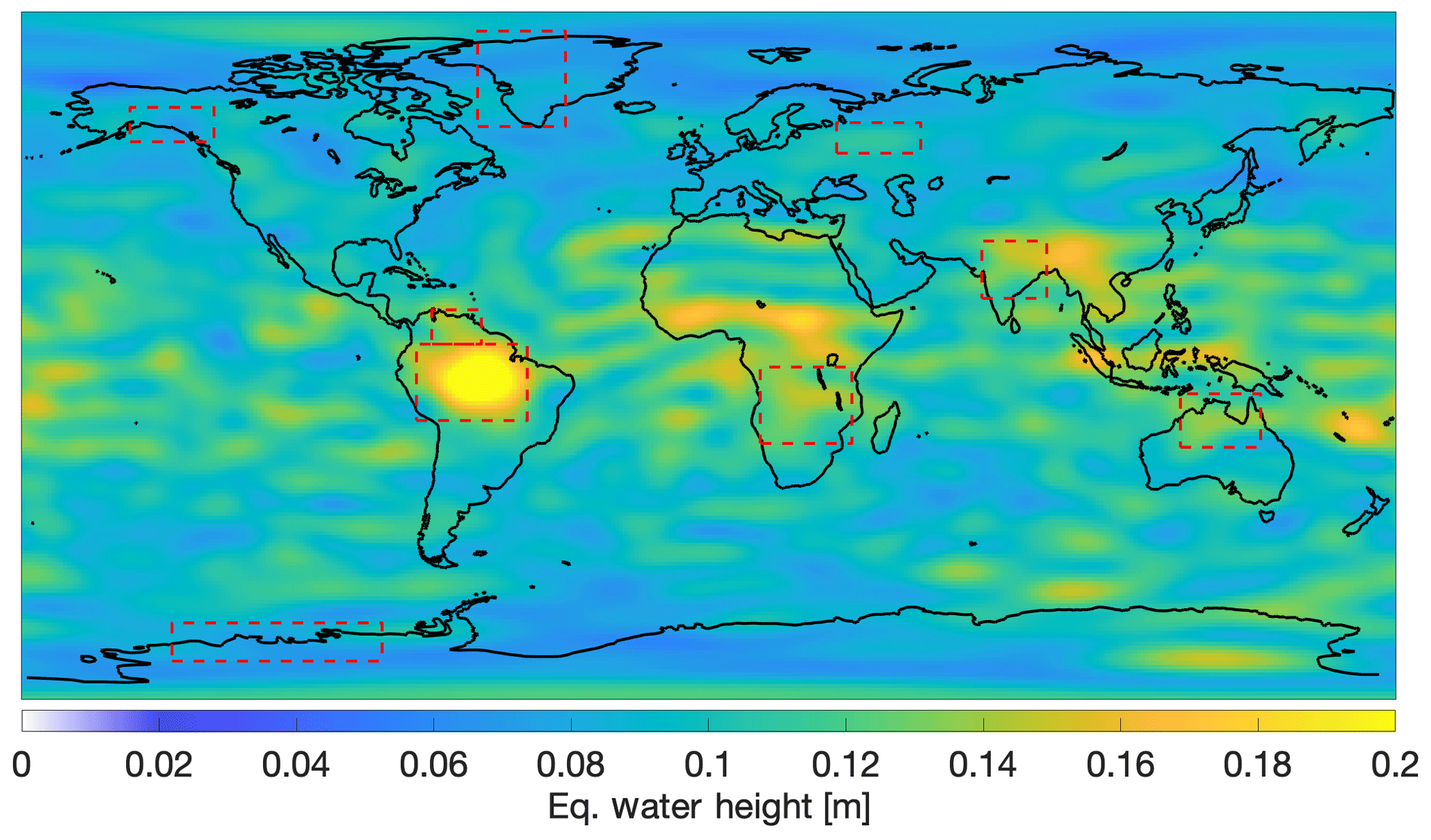
Figure 26 Signal variability for Swarm during the period between December 2013 and March 2019, under 750 km Gaussian smoothing.

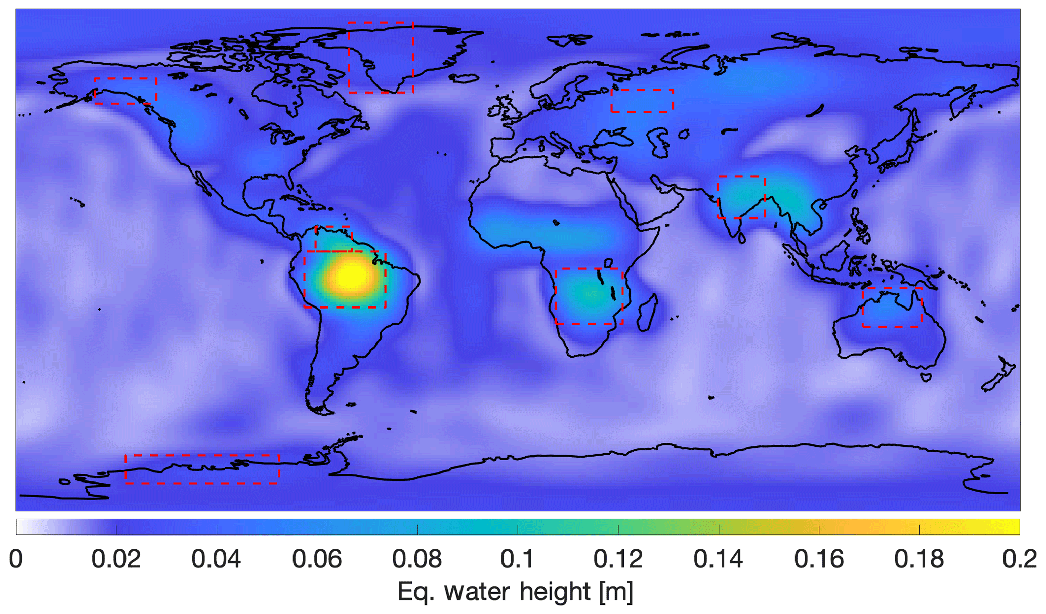
Figure 27 Signal variability for GRACE during the Swarm period December 2013 to March 2019, including the earliest GRACE-FO solutions, under 750 km Gaussian smoothing.

Looking at the variability in the GRACE models over the same periods, Fig. 27 (produced in a way consistent with Fig. 26), there is no obvious signature of geomagnetic effects. Additionally, the variability over the oceans is very small, in comparison to land areas.

3.5.3 Large storage basins

In this section, we present time series of Swarm and GRACE average EWH over the areas highlighted in Figs. 26 and 27. Unlike the previous sections, the GRACE signal (relative to GGM05C) is calculated from the monthly RL06 CSR solutions, after 750 km smoothing and the usual C_2,0 replacement. The trend (and bias) is co-estimated with yearly and semi-yearly sine and cosine periods, in order to be insensitive to phase differences at the beginning and end of the period under analysis. Instead of disclosing the constant term in the polynomial and sinusoidal regression, we prefer to report the average over the period under analysis as a measure of a constant bias.

We illustrate these time series with the example of Greenland and the Amazon, in Figs. 28 and 29, respectively. The remaining time series can be found in Appendix E. As was the case with the analysis of the low degrees, the time series are less smooth than GRACE, as a result of the increased influence of errors. In spite of this, the Swarm time series follows GRACE closely, with a correlation coefficient of 0.83 and 0.95 for Greenland and the Amazon, respectively. The trend is overestimated by −0.6 and −1.12 cm yr⁻¹, respectively, mainly as a result of the higher errors before mid-2015. Swarm also agrees with the GRACE-FO observation that the Greenland ice mass loss slowed down during the winter of 2018–2019, since both Swarm and GRACE-FO lines are above the linear interpolation. During the summer of 2019, the ice mass loss in Greenland accelerated, which is consistently observed by both Swarm and GRACE. In the case of the Amazon basin, the GRACE-FO months agree particularly well with Swarm.

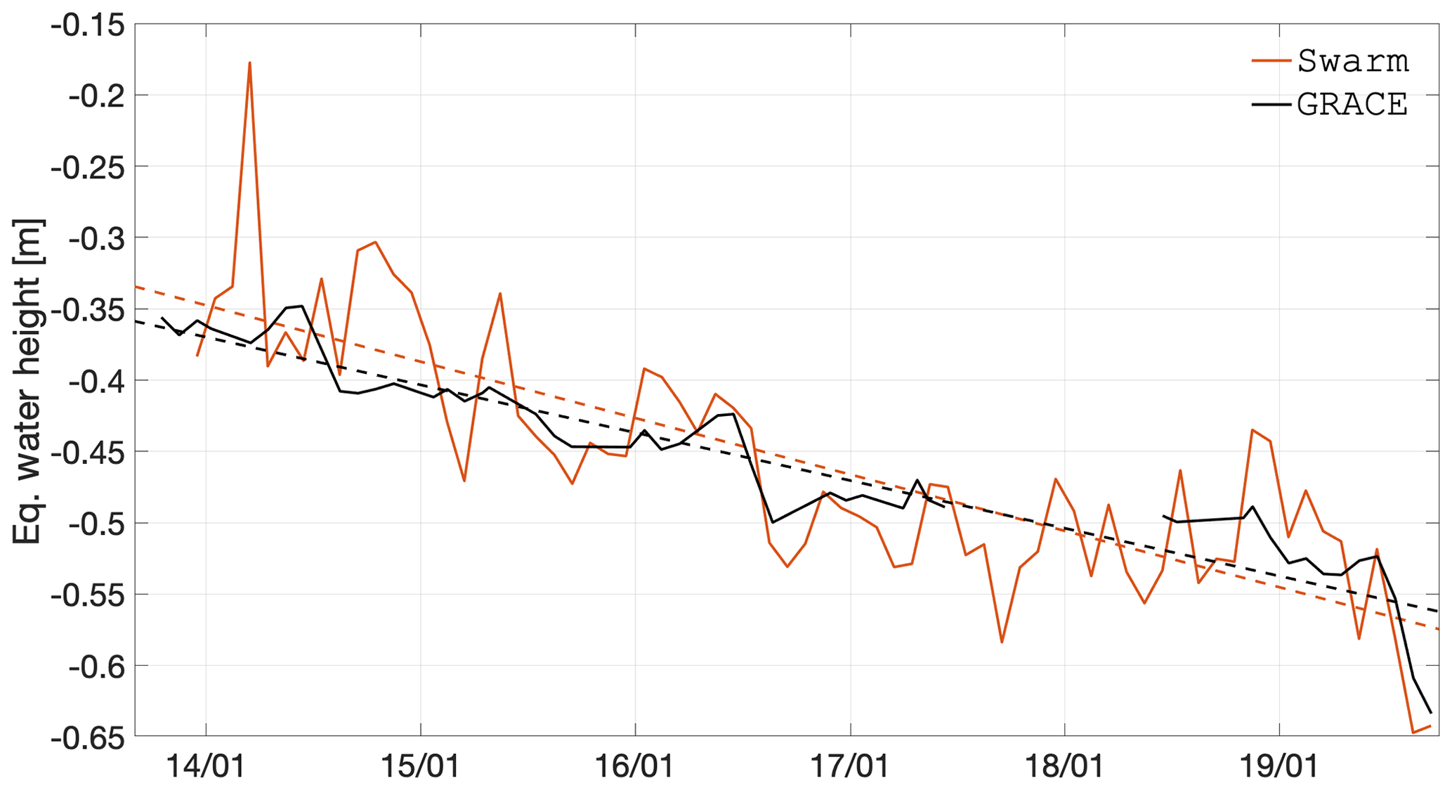
Figure 28 Time series of EWH for the western Greenland region (latitude 60 to 85^∘, longitude −60 to −37^∘).

Table 7 Bias and trend agreement, as well as correlation coefficient between the GRACE and Swarm time series for the selected basins, over the complete Swarm period (December 2013 to September 2019).

Table 7 provides an overview of the statistics derived from the time series of all analysed basins. The Swarm and GRACE time series agree on their average values between −1.50 cm (Amazon) and 0.78 cm (Orinoco), on their trend between −1.16 cm yr⁻¹ (Orinoco) and 0.36 cm yr⁻¹ (Congo and Zambezi) and on their correlation coefficient between 0.65 (Volga) and 0.95 (Amazon). All regions show a variety of values in their statistics, thus making it difficult to immediately identify which one is best observed. For example, although the Amazon time series shows the largest trend difference (in absolute value), it also has the highest correlation coefficient. If the period before mid-2015 is ignored, these statistics improve substantially (not shown).

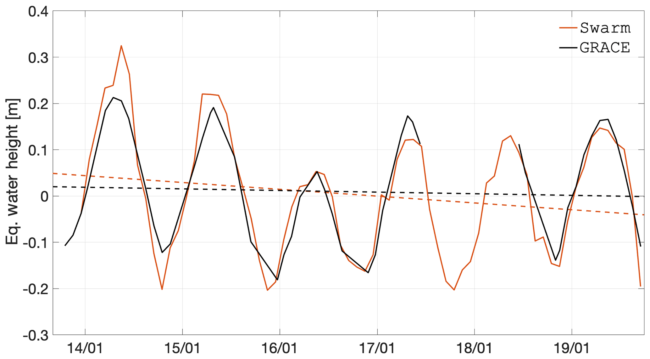
Figure 29 Time series of EWH for the Amazon basin (latitude −17 to 3^∘, longitude −76 to −47^∘).

Over the nine basins presented in this section and in Appendix E, the Swarm rms difference with respect to GRACE is 0.91 cm in terms of temporal mean and 0.76 cm yr⁻¹ in terms of trend and shows an average correlation coefficient of 0.79 (bottom of Table 7). Note that the complete Swarm period was considered in deriving these statistics and represents a conservative estimate of the accuracy of Swarm if the early period before mid-2015 is discarded.

4 Data availability

The Swarm monthly models are distributed on a quarterly basis at ESA's Earth Swarm Data Access (at https://swarm-diss.eo.esa.int/, last access: 5 June 2020, follow “Level2longterm” and then “EGF”) and at the International Centre for Global Earth Models (http://icgem.gfz-potsdam.de/series/02_COST-G/Swarm, last access: 5 June 2020), as well as identified with the DOI https://doi.org/10.5880/ICGEM.2019.006 (Encarnacao et al., 2019).

5 Conclusions

We present Swarm GFMs resulting from the combination of four individual solutions computed from different gravity field estimation approaches: celestial mechanics approach (CMA), decorrelated acceleration approach (DAA), improved energy balance approach (IEBA), and short-arc approach (SAA). Two approaches (CMA and IEBA) exploit the KO solutions produced at AIUB and the other two (DAA and SAA) the KOs produced at IfG. The combination is done at the solution level, weighted by VCE; for the sake of brevity, we refer to Teixeira da Encarnação and Visser (2019) to demonstrate that our combination produces Swarm models in better agreement with GRACE than if the combination is done at the NEQ level.

We test the added value of KB in the quality of the Swarm GFM, when compared to the long wavelength signal recovered by GRACE, by computing seven GFMs during periods of different data quality. We demonstrate that the largest changes in the results appear during early 2015 (high ionospheric activity, before improvements in Swarm's GPS receivers) that translate into a slight deterioration of the quality of the Swarm solutions; see Table 5. For the 5 months analysed in 2016, considering two KO solutions, any improvement is minimal (0.1 to 0.2 mm geoid height, in five cases), negligible (in two cases), or slightly worse (0.1 mm in three cases). We conclude that any common errors that would be eliminated in the KB solutions are already (mostly) corrected in the KOs. For this reason, our Swarm GFMs do not consider KBs.

Another test regarding the added value of additional data took the form of including Swarm C non-gravitational accelerations. We compared the three-satellite Swarm solution produced considering the DAA and non-gravitational accelerations acting on Swarm C represented by the TUD and ASU non-gravitational acceleration models, in addition to exploiting the accelerometer measurements. Since the Swarm A and B satellites do not produce usable accelerometer readings, they are represented by the ASU model exclusively. The results indicate that the accelerometer observations are only beneficial in those cases when the amplitude of the non-gravitational accelerations acting on Swarm C are of higher amplitude than in quiet periods in solar activity, such as is the case since 2016. This may be the result of the potentially lower quality of the calibrated accelerations, caused by the lower SNR in the accelerometer observations.

Regarding the topic of non-gravitational accelerations in the processing of GPS-driven GFMs, we would like to comment on the results of Ditmar et al. (2006) and Ditmar et al. (2008), who demonstrated that non-gravitational accelerations are not needed for gravity field estimation and the quality of the GPS observations (and the resulting KOs) are the main drivers of the quality of the GFMs. Within our project, each AC is free to elect whatever processing strategy they deem to be most beneficial to their individual solutions, which is assessed internally. For example, AIUB has determined that the use of daily and 15 min piecewise-constant empirical parametrization does not require any modelling of non-gravitational accelerations. In the case of ASU, who exploit a dedicated decorrelation procedure (which is a frequency-dependent noise whitening procedure), their solutions benefit from drag, EARP, and EIRP models. Essentially, the inclusion of frequency-dependent data weighting (FDDW) is not within immediate reach to all ACs, in which case other processing strategies seem to produce comparable solution quality. In summary, we do not wish to contest previous results on this topic but clarify the differences in our processing choices.

We quantify the different quality of the various individual solutions and demonstrate that all have the potential to contribute positively to the quality of the combined Swarm time series of GFMs. We additionally explain that our approach to combine the individual GFMs at the solution level considering VCE weights is an effective way of overcoming the difficulty in combining solutions at the NEQ level when the corresponding normal matrices represent errors of different type, formal and calibrated in our case (Teixeira da Encarnação and Visser, 2019).

Masking the Swarm data separately over ocean and land, we demonstrate Swarm's combined models' ability to measure land mass transport processes, with a comparable spatial variability of the Swarm–GRACE residual to that of the GRACE signal, for the post mid-2015 period. Over the ocean areas, the spatial rms of the difference between Swarm and GRACE is always larger than the spatial rms of the latter. To resolve the oceanic signal, the Swarm data required a more intense Gaussian smoothing, with a radius of 3000 km.

We analyse the signal content of the Swarm models in terms of time series of the low degrees, spatial patterns of the temporal signal variability, and time series of large storage basins. Comparing the time series of isolated SH coefficients, we show that the Swarm data generally have a more erratic temporal evolution with sudden month-to-month variations. We attribute this particularity to the lower accuracy of the GPS observations as gravimetric data, compared to GRACE's K-band ranging (KBR) data. We also illustrate features in the Swarm data that are not captured by the GRACE climatological model, but confirmed by the GRACE and GRACE-FO data, notably the atypical deviation around early 2016 in the $C_{\mathrm{5},-\mathrm{1}}$ coefficient. By plotting the spatial patterns in the temporal variability of the Swarm data, we bring into evidence the strong signature over the geomagnetic Equator, showing strong meridional stripes, and over the south magnetic pole (but not on the north magnetic pole). In spite of this artefact, the strong mass variability over the Amazon basin is clearly visible. With regard to the time series of mass changes over large storage basins, Swarm agrees on average with GRACE (the climatological model was not relevant to this analysis) at 0.91  cm in terms of temporal mean, 0.76 cm yr⁻¹ in terms of trend, and 0.79 correlation coefficient over the nine basins we considered. We show that Swarm agrees with the observation of GRACE-FO that the ice mass loss over Greenland seems to have slowed down during late 2018 and accelerated in the summer of 2019, in spite of the heavy signal dilution caused by the necessary smoothing to reduce the errors in the Swarm models. Although our Swarm models are already in production mode, we are considering several options to improve their quality. Given the high sensitivity of the KOs to ionospheric activity, we plan to focus our efforts to improve the weighting of the GPS observations (Dahle et al., 2017; Kermarrec et al., 2018; Schreiter et al., 2019). We also plan to decrease the disagreement between the individual solution produced at OSU and those at other ACs by including advanced algorithms for reducing the effects of jumps and the amplification of high-frequency noise in the differentiation of the KO positions into velocities.

Appendix A: Kinematic orbits

A1 Delft University of Technology

Software:	GPS High precision Orbit determination
	Software Tool (van Helleputte, 2004; Wermuth et al., 2010)
Differencing scheme:	Undifferenced
Linear combination:	Ionosphere-free
GPS observations:	Code and carrier phase
Estimator:	Bayesian-weighted LS
Arc length:	30 h
Data weighting:	a priori weights equal to 1 m and 1 mm for code and phase observations (resp.)
Transmitter PCV:	Official IGS08 ANTEX up to day 17/028, official IGS14 ANTEX from day 17/029 on
Receiver PCV:	Empirically determined from stacking of reduced-dynamic POD residuals with 1∘ binning
Data screening:	Minimum SNR of 10, minimum of six GPS satellites, code and phase outlier editing threshold of
	2 m and 3.5 cm, respectively, 1 m or larger difference between estimated KO positions and with
	reduced-dynamic precise science orbit (PSO)
Earth precession model:	International Astronomical Union (IAU) 1976 (Lieske et al., 1977)
Earth nutation model:	IAU 1980 (Seidelmann, 1982)
Earth orientation model:	Centre for Orbit Determination in Europe (CODE) final Earth rotation parameters (ERP)

A2 Astronomical Institute of the University of Bern

Software:	Bernese v5.3 (Dach et al., 2015; Jäggi et al., 2006)
Differencing scheme:	Undifferenced
Linear combination:	Ionosphere-free
GPS observations:	Carrier phase
Estimator:	Batch LS
Arc length:	24 h
Data weighting:	Not applicable (n/a)
Transmitter PCV:	Official IGS08 ANTEX up to day 17/028, official IGS14 ANTEX from day 17/029 on
Receiver PCV:	Stacking of residuals from reduced-dynamic precise orbit determination (POD) of
	approx. 120 d, nine iterations, 1∘ binning
Data screening:	2 cm s−1 or larger time differences of the geometry-free linear combination of
	L1B GPS carrier phase observations
Earth precession model:	International Earth Rotation Service (IERS) 2010 Conventions (Petit and Luzum, 2010)
Earth nutation model:	IERS 2010 Conventions (Petit and Luzum, 2010)
Earth orientation model:	CODE final ERP

A3 Institute of Geodesy Graz

Software:	GROOPS
Differencing scheme:	None
Linear combination:	None (the ionospheric influence is co-estimated)
GPS observations:	Code and carrier phase
Estimator:	LS
Arc length:	24 h
Data weighting:	Elevation and azimuth-dependent, epoch-wise VCE
Transmitter PCV:	Empirical, estimated from 5.5 years of data, including data from several LEO missions (GRACE,
	Jason 2 & 3, MetOp-A & MetOp-B, Sentinel 3A, Swarm, TanDEM-X, TerraSAR-X) (Zehentner, 2016)
Receiver PCV:	Empirical, spherical harmonics (maximum D/O 60), derived from 38 months of data
Data screening:	Implicit in VCE
Earth precession model:	IAU 2006/2000A precession–nutation model (Petit and Luzum, 2010)
Earth nutation model:	IAU 2006/2000A precession–nutation model (Petit and Luzum, 2010)
Earth orientation model:	IERS Earth Orientation Parameter (EOP) 08 C04 (Petit and Luzum, 2010)

A4 Common

Carrier phase ambiguities:	Float
Receiver clock corrections:	Co-estimated
Sampling rate:	10 or 1 s (depending on L1B GPS data)
Elevation cut-off angle:	0∘
GPS orbits and clocks:	Final orbits and 5 s clocks of Centre for Orbit Determination in Europe (Dach et al., 2017)
Swarm attitude:	L1B attitude data

Appendix B: Kinematic baselines

B1 Delft University of Technology

Software:	Multiple-satellite orbit determination using Kalman filtering (van Barneveld, 2012)
Linear combination:	n/a (the ionospheric frequency-dependent influence is modelled)
Estimator:	Iterative EKF
Carrier phase ambiguities:	Integer, using the least-squares ambiguity de-correlation adjustment method (Teunissen, 1995)
Receiver PCV:	Empirical phase centre variations (PCVs) and code residual variations (CRVs);
	maps are estimated a priori for each GPS frequency

B2 Astronomical Institute of the University of Bern

Software:	Bernese (Dach et al., 2015; Jäggi et al., 2006), development version
Linear combination:	Ionosphere-free
Estimator:	LS
Carrier phase ambiguities:	Wide-lane and narrow-lane integer ambiguity fixing with the Melbourne–Wübbena combination
	and the ionosphere-free linear combination, respectively
Receiver PCV:	Empirical

B3 Common

Differencing scheme:	Double-differenced
GPS observations:	Code and carrier phase
Carrier phase ambiguities:	Integer

Appendix C: Gravity field models

C1 Astronomical Institute of the University of Bern

Software:	Bernese v5.3 (Dach et al., 2015; Jäggi et al., 2006)
Approach:	celestial mechanics approach (Beutler et al., 2010)
Reference GFM:	AIUB GRACE-only static model, version 3 (Jäggi et al., 2011)
Empirical parameters:	Daily and 15 min piecewise-constant (constrained)
Drag model:	None
EARP and EIRP models:	None
Non-tidal model:	Atmosphere and Ocean De-aliasing Level 1B (Flechtner, 2011)
Ocean tidal model:	2011 Empirical Ocean Tide model (Savcenko and Bosch, 2012)
Permanent tide system:	Tide-free

C2 Astronomical Institute Ondřejov

Software:	Developed in-house
Approach:	Decorrelated acceleration approach (Bezdek et al., 2014)
Reference GFM:	ITG GRACE-only static model, 2010 (Mayer-Gürr et al., 2010)
Empirical parameters:	Daily constant-piecewise
Drag model:	US Naval Research Laboratory Mass Spectrometer and Incoherent Scatter Radar atmospheric model
	(Picone et al., 2002)
EARP and EIRP models:	Knocke et al. (1988)
Non-tidal model:	Atmosphere and Ocean De-aliasing Level 1B (Dobslaw et al., 2017)
Ocean tidal model:	2004 finite element solution (Lyard et al., 2006)
Permanent tide system:	Tide-free

C3 Institute of Geodesy Graz

Software:	GROOPS
Approach:	Short-arc approach (Mayer-Gürr, 2006)
Reference GFM:	GOCO release 05 satellite-only gravity field model (Mayer-Gürr, 2015)
Empirical parameters:	Piecewise linear for each arc (ranging from 15 to 45 min)
Drag model:	Jacchia–Bowman 2008 (Bowman et al., 2008)
EARP and EIRP models:	Rodriguez-Solano et al. (2012)
Non-tidal model:	Atmosphere and Ocean De-aliasing Level 1B RL06 (Dobslaw et al., 2017)
Ocean tidal model:	2014 finite element solution (Carrere et al., 2015)
Permanent tide system:	Zero tide

C4 Ohio State University

Software	Developed in-house
Approach:	Improved energy balance approach (Shang et al., 2015)
Reference GFM:	GRACE Intermediate Field 48 (Ries et al., 2011) up to degree and order (D/O) 200
Empirical parameters:	Second-order polynomial every 3 h, 1-CPR sinusoidal every 24 h
Regularization:	None
Drag model:	US Naval Research Laboratory Mass Spectrometer and Incoherent Scatter Radar atmospheric model
	(Picone et al., 2002)
EARP and EIRP models:	Knocke et al. (1988)
Non-tidal model:	Atmosphere and Ocean De-aliasing Level 1B (Flechtner, 2011)
Ocean tidal model:	2011 empirical ocean tide model (Savcenko and Bosch, 2012)
Permanent tide system:	Tide-free

C5 Common

Atmospheric tidal model:	Biancale and Bode (2006)
Solid Earth tidal model:	IERS2010
Pole tidal model:	IERS2010
Ocean pole tidal model:	IERS2010
Third-body perturbations:	Sun, Moon, Mercury, Venus, Mars, Jupiter, and Saturn, following the JPL Planetary and
	Lunar Ephemerides (Folkner et al., 2014)
C2,0 coefficient:	Estimated alongside other coefficients

Appendix D: Time series of zonal coefficients

Figures D1–D3 illustrate the time series for the zonal coefficients of degrees 3 to 6, respectively.

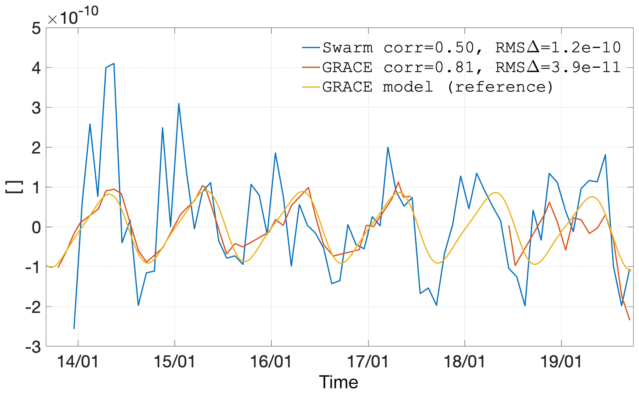
Figure D1 Coefficient C_3,0 as observed by GRACE and Swarm, as well as represented by the GRACE climatological model.

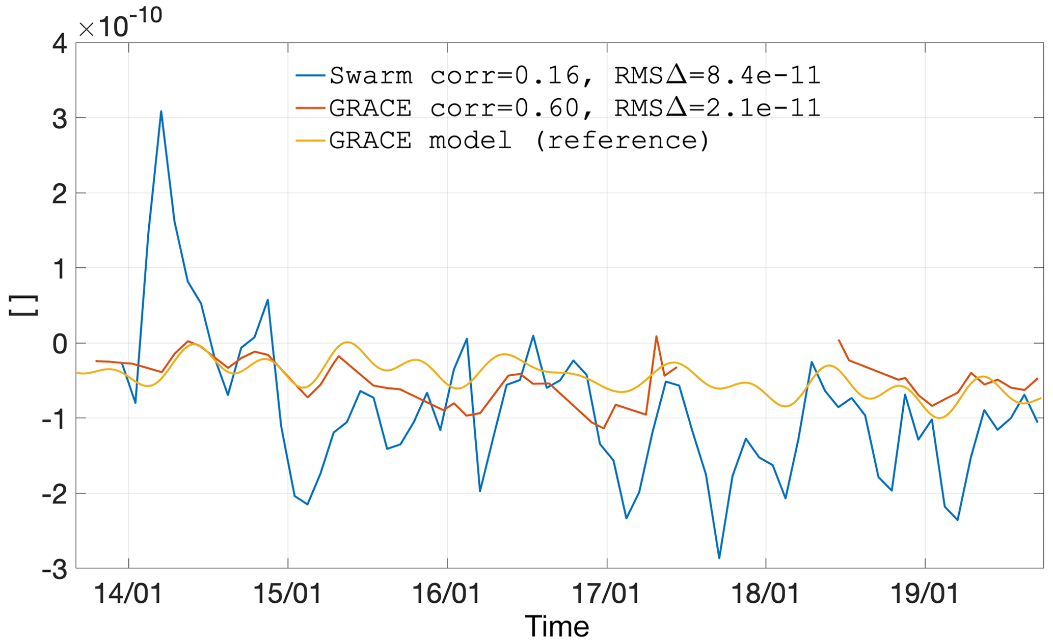
Figure D2 Coefficient C_4,0 as observed by GRACE and Swarm, as well as represented by the GRACE climatological model.

The zonal coefficient of degree 3 is an interesting case because both Swarm and GRACE-FO observe a phase shift during late 2018, relative to the climatological model, which is well in phase with GRACE for the non-GRACE-FO period (2003–2017). Swarm already captures this phase shift possibly as early as mid-2017, although the noisy character of the Swarm time series weakens this type of statement.

The zonal coefficient of degree 4 is one of the few examples where the Swarm time series shows a clear bias relative to GRACE and the climatological model, after 2017 in this case. As was the case for C_2,1, we cannot explain such behaviour.

The zonal coefficient of degree 5 is an example of excellent agreement between all three time series. Swarm still shows the characteristic noise, as well as a higher overall disagreement before mid-2015. These are features intrinsic to our Swarm solutions.

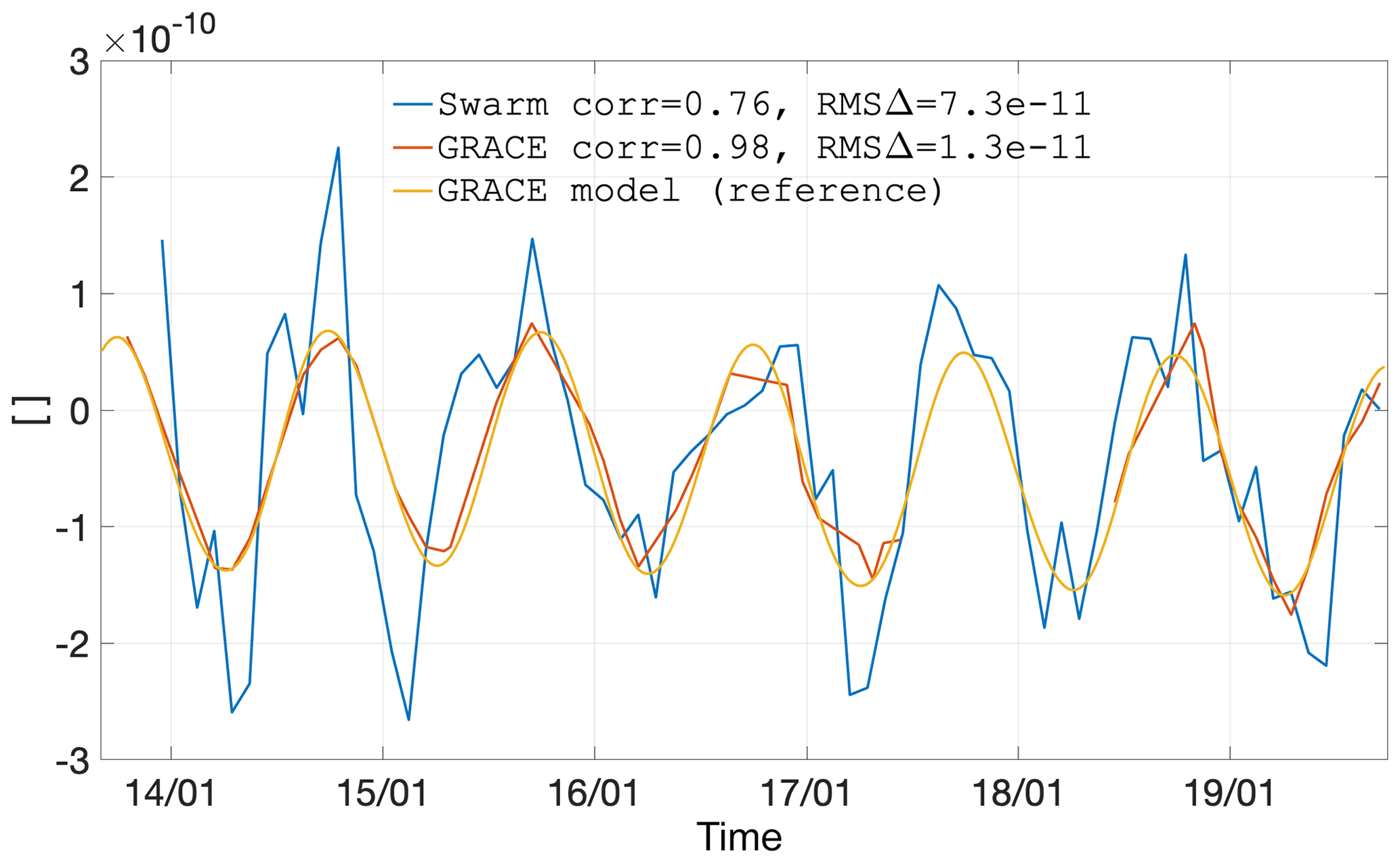
Figure D3 Coefficient C_5,0 as observed by GRACE and Swarm, as well as represented by the GRACE climatological model.

Appendix E: Storage basin time series

Figure E1 Time series of EWH for Alaska (latitude 56 to 65^∘, longitude −151 to −129^∘).

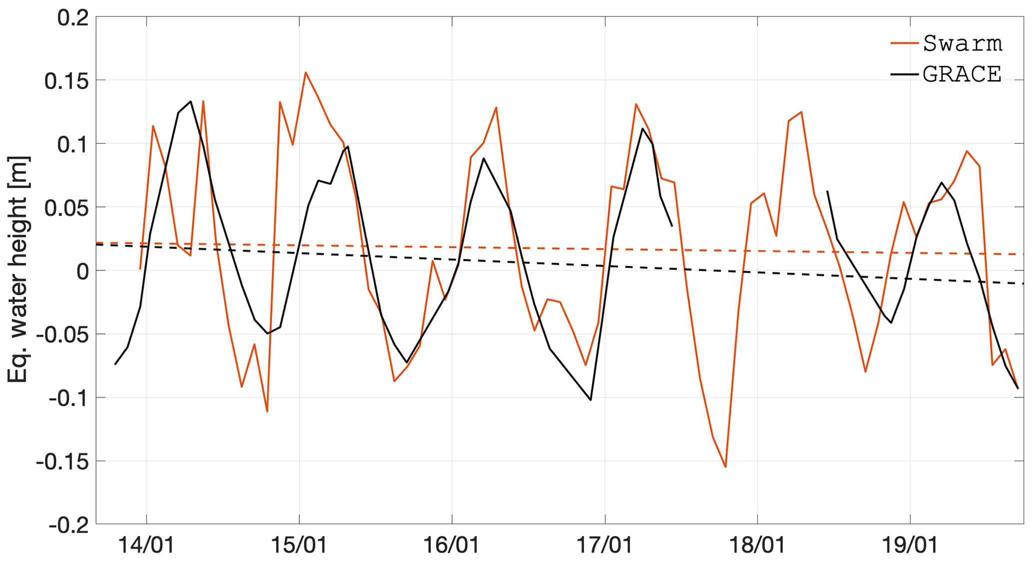
Figure E2 Time series of EWH for the Congo and Zambezi basins (latitude −23 to −3^∘, longitude 14 to 38^∘).

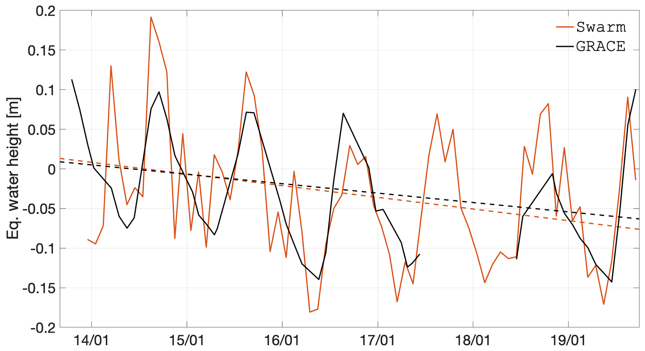
Figure E3 Time series of EWH for the Ganges–Brahmaputra basin (latitude 15 to 30^∘, longitude 72 to 89^∘).

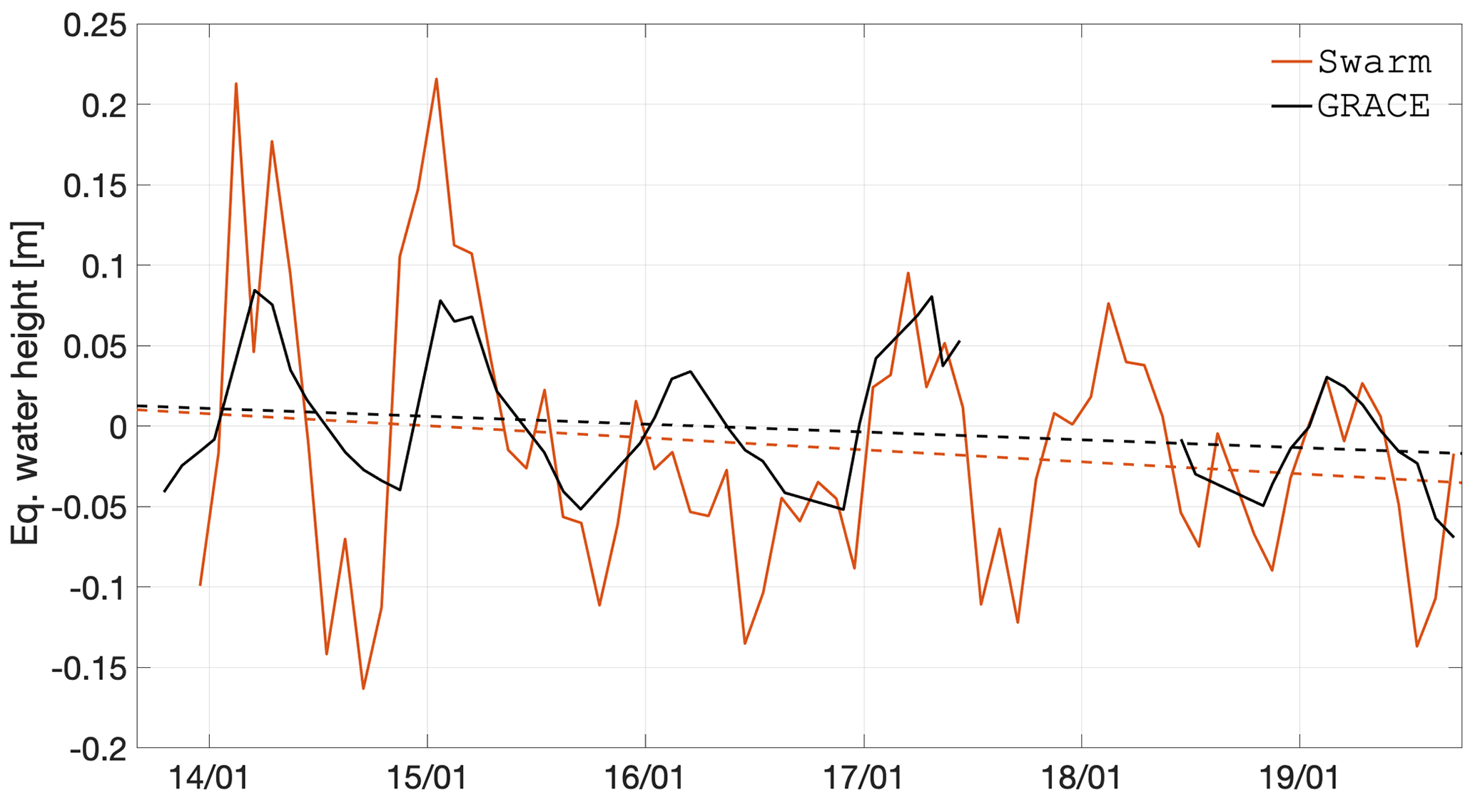
Figure E4 Time series of EWH for the northern Australia region (latitude −24 to −10^∘, longitude 124 to 145^∘).

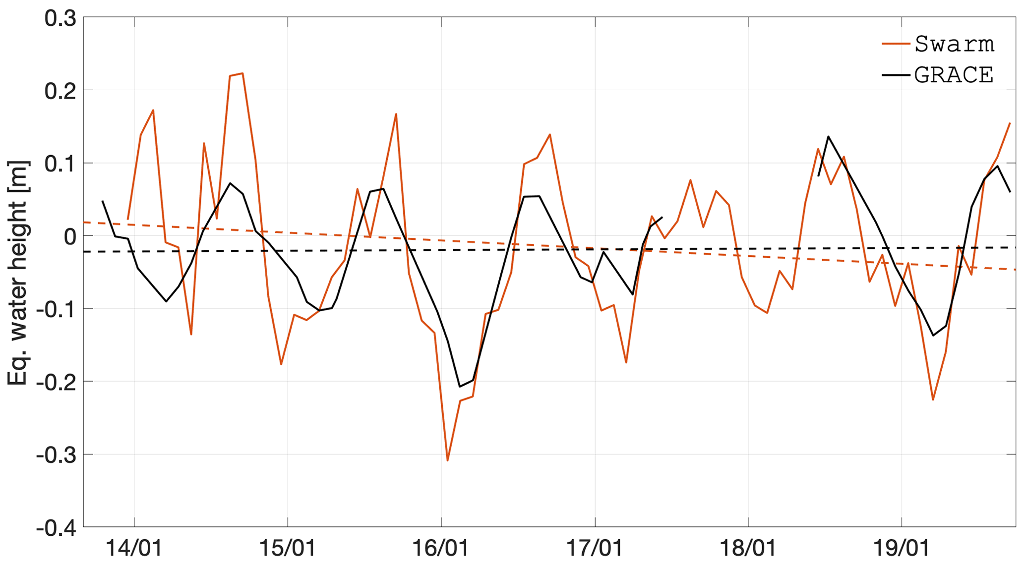
Figure E5 Time series of EWH for the Orinoco basin (latitude −3 to 12^∘, longitude −72 to −59^∘).

Figure E6 Time series of EWH for the Volga basin (latitude 53 to 61^∘, longitude 34 to 56^∘).

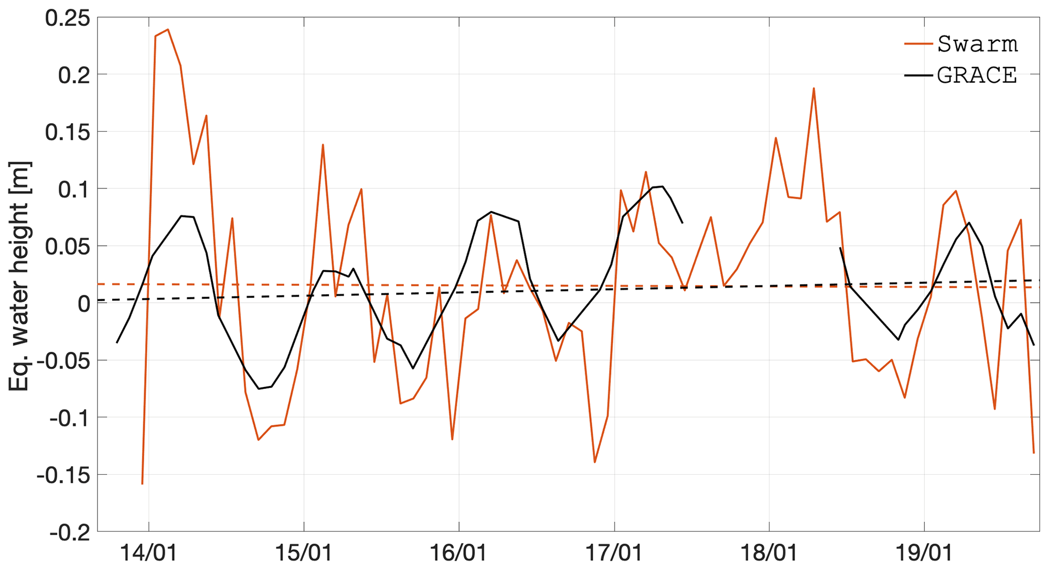
Figure E7 Time series of EWH for the western Antarctica region (latitude −80 to −70^∘, longitude −140 to −85^∘).

Appendix F: Abbreviations

3D	Three-dimensional
AA	Acceleration approach
DAA	Decorrelated acceleration approach
AC	Analysis centre
AIUB	Astronomical Institute of the University of Bern, Switzerland
AIUB-GRACE03S	AIUB GRACE-only static model, version 3
AOD1B	Atmosphere and Ocean De-aliasing Level 1B
AOD1B-RL06	Atmosphere and Ocean De-aliasing Level 1B RL06
ANGARA	Analysis of non-gravitational accelerations due to radiation pressure and aerodynamics
ASU	Astronomical Institute (Astronomický ústav), AVCR, Ondřejov
AVCR	Czech Academy of Sciences (Akademie ved Ceské Republiky), Czech Republic
CHAMP	Challenging Mini-Satellite Payload
CODE	Centre for Orbit Determination in Europe
CMA	Celestial mechanics approach
CoM	Centre of mass
COST-G	Combination Service of Time-variable Gravity Fields
CPR	Cycle per revolution
CRV	Code residual variation
CSR	Center for Space Research, UT Austin, USA
D/O	Degree and order
DAA	Decorrelated acceleration approach
DD	Double-differenced
DISC	Data, innovation and science cluster
DOI	Digital object identifier
DWM07	Disturbance Wind Model 07
EARP	Earth albedo radiation pressure
EGSIEM	European Gravity Service for Improved Emergency Management, EU Horizon 2020
EIRP	Earth infrared radiation pressure
EKF	Extended Kalman filter
EBA	Energy balance approach
EOT	Empirical ocean tide model
EOT11a	2011 empirical ocean tide model
EWH	Equivalent water height
EOP	Earth orientation parameter
ERBE	Earth Radiation Budget Experiment
ERP	Earth rotation parameters
ESA	European Space Agency
EU	European Union
FDDW	Frequency-dependent data weighting
FES	Finite element solution global tide model
FES2004	2004 finite element solution
FES2014	2014 finite element solution
GFM	Gravity field model
GHOST	GPS High precision Orbit determination Software Tool
GGM05C	Combined GRACE Gravity Model 05
GIF48	GRACE Intermediate Field 48
GOCE	Gravity Field and Steady-State Ocean Circulation Explorer
GOCO	Gravity Observation Combination
GOCO05S	GOCO release 05 satellite-only gravity field model
GPS	Global Positioning System
GRACE	Gravity Recovery and Climate Experiment
GRACE-FO	GRACE Follow-On
GROOPS	Gravity Recovery Object Oriented Programming System
hl-SST	High-low satellite-to-satellite tracking

HWM07	Horizontal Wind Model 07
IAG	International Association of Geodesy
IAU	International Astronomical Union
ICGEM	International Centre for Global Earth Models
IEBA	Improved energy balance approach
IERS	International Earth Rotation Service
IERS2010	IERS Conventions 2010
IfG	Institute of Geodesy, TUG, Graz
IGFS	International Gravity Field Service
IR	Infrared radiation
ISR	Inter-satellite range
ITG	Institut für Geodäsie und Geoinformation, Germany
ITSG	Institute of Theoretical Geodesy and Satellite Geodesy
ITG-Grace2010s	ITG GRACE-only static model, 2010
ITSG-Grace2016	ITSG GRACE-only model, 2016
JB2008	Jacchia-Bowman 2008
JPL	Jet Propulsion Laboratory, USA
JPL-PLE	JPL Planetary and Lunar Ephemerides
KB	Kinematic baseline
KBR	K-band ranging
KO	Kinematic orbit
L1A	Level 1A data
L1B	Level 1B data
L2	Level 2 data
L2PS	Level 2 processing system
LAMBDA	Least-squares ambiguity de-correlation adjustment
LEO	Low-Earth orbit
ll-SST	Low–low satellite-to-satellite tracking
LoS	Line of sight
LS	Least squares
MAD	Median absolute deviation
MODK	Multiple-satellite orbit determination using Kalman filtering
n/a	Not applicable
NEQ	Normal equation
NRLMSISE	US Naval Research Laboratory Mass Spectrometer and Incoherent Scatter Radar atmospheric model
NRTDM	Near Real-Time Density Model
OSU	Ohio State University
PCV	Phase centre variation
POD	Precise orbit determination
PSO	Precise or post-processed science orbit
RINEX	Receiver Independent Exchange Format
RL05	Release 5
RL06	Release 6
Rms	Root mean square
SAA	Short-arc approach
SC	Stokes coefficient
SH	Spherical harmonic
SLR	Satellite laser ranging
SNR	Signal-to-noise ratio
SRP	Solar radiation pressure
SD	Standard deviation
TUD	Delft University of Technology, Netherlands
TUG	Graz University of Technology, Austria
UT Austin	University of Texas at Austin
USA	United States of America
VEA	Variational equations approach
VCE	Variance component estimation
ZD	Zero-differenced