the Creative Commons Attribution 4.0 License.
the Creative Commons Attribution 4.0 License.
 | 06 Nov 2019
A new merge of global surface temperature datasets since the start of the 20th century
Xiang Yun
Boyin Huang
Jiayi Cheng
Wenhui Xu
Shaobo Qiao
Global surface temperature (ST) datasets are the foundation for global climate change research. Several global ST datasets have been developed by different groups in NOAA NCEI, NASA GISS, UK Met Office Hadley Centre & UEA CRU, and Berkeley Earth. In this study, a new global ST dataset named China Merged Surface Temperature (CMST) was presented. CMST is created by merging the China-Land Surface Air Temperature (C-LSAT1.3) with sea surface temperature (SST) data from the Extended Reconstructed Sea Surface Temperature version 5 (ERSSTv5). The merge of C-LSAT and ERSSTv5 shows a high spatial coverage extended to the high latitudes and is more consistent with a reference of multi-dataset averages in the polar regions. Comparisons indicated that CMST is consistent with other existing global ST datasets in interannual and decadal variations and long-term trends at global, hemispheric, and regional scales from 1900 to 2017. The CMST dataset can be used for global climate change assessment, monitoring, and detection. The CMST dataset presented here is publicly available at https://doi.org/10.1594/PANGAEA.901295 (Li, 2019a) and has been published on the Climate Explorer website of the Royal Netherlands Meteorological Institute (KNMI) at http://climexp.knmi.nl/select.cgi?id=someone@somewhere&field=cmst (last access: 11 August 2018; Li, 2019b, c).
- Article
(10823 KB) - Full-text XML
- BibTeX
- EndNote


The long-term trend in the global mean surface temperatures (GMSTs) is a common measure in observing the change of climate. Therefore, the biases of the observed surface temperature (ST) dataset, particularly the sampling bias of high-latitude stations, have received much attention in the past few years (Anderson, 2011; Church et al., 2013; Cowtan and Way, 2014; Jones and Moberg, 2003; Jones, 2016; Li et al., 2009, 2017, 2019a, b; Simmons et al., 2017; J. Huang et al., 2017). The optimization and improvement of observed climate data as a reference base for climate change research and verification benchmark for other climatic data products is a long-term task.
A total of four global land surface air temperature (LSAT) observation series and three global ST series were presented by the Intergovernmental Panel on Climate Change (IPCC, 2013) a few years ago. These four LSATs include the Climatic Research Unit (CRU) land surface air temperature, version 4 (CRUTEM4; Jones et al., 2012; Osborn and Jones, 2014); Global Historical Climatology Network-monthly (GHCNm) temperature, version 3 (GHCNm v3; Lawrimore et al., 2011; Peterson et al., 1997); Goddard Institute for Space Studies analysis of land surface air temperature (GISS; Hansen et al., 2010); and Berkeley Earth Surface Temperature group land temperature (Berkeley; Rohde et al., 2013). The three global ST series are the Met Office Hadley Centre and Climatic Research Unit Temperature version 4 (HadCRUT4; Morice et al., 2012); Merged Land–Ocean Surface Temperature (MLOST; Vose et al., 2012); and Goddard Institute for Space Studies Surface Temperature Analysis (GISTEMP; Hansen et al., 2010).
These global ST data products have been updated over the past few years since the publication of IPCC (2013). For instance, NOAA has updated the Extended Reconstructed Sea Surface Temperature (ERSST) version 3 to ERSSTv4 (Huang et al., 2015) and ERSSTv5 (B. Huang et al., 2017), updated LSAT dataset GHCNm v3 to GHCNm v4 (Menne et al., 2018), and renamed MLOST to NOAA Global Surface Temperature (NOAAGlobalTemp). GISTEMP has updated its SST component to ERSSTv5 (B. Huang et al., 2017). CRUTEM has been updated to CRUTEM4.6. The Met Office updated the Hadley Centre SST to version 3 (HadSST3) using the median of 100 ensemble members. And lastly, the Berkeley team used the median of the HadSST3 ensemble to form the Berkeley Earth Surface Temperature (BEST) dataset.
The products' updates are based on the advanced knowledge of data analysis methodology or improved data availability. In general, the GMST has continuously been improved by the increased number and area coverage of observational data over land (LSAT) and oceans (SST). There are two aspects to improving the LSAT datasets: firstly, increasing the data coverage and density of stations, especially in key areas with sparse observations. For example, the number of observations is increased in both C-LSAT (Xu et al., 2018) and GHCNm v4 (Menne et al., 2018) using newly released International Surface Temperature Initiative (ISTI) datasets (Thorne et al., 2011) or datasets through regional cooperation with Asian countries such as Vietnam and South Korea. Coverage of datasets increases with a larger number of observations, hence reducing the sampling biases, particularly for high-latitude areas (polar regions) and observation-sparse regions (such as South America and Africa). The second aspect is improving the accuracy of regional climate changes. For example, the latest C-LSAT (Xu et al., 2018) has integrated more regional homogenization results, especially over China (Li et al., 2009; Xu et al., 2013), East Asia, Europe, Australia (Trewin, 2013), and Canada (Vincent et al., 2012). On the other hand, there are also two aspects to improving the SST datasets: (1) integration of much better raw observational data and (2) replacing a single analysis with multi-member ensemble analyses. For instance, ERSSTv5 uses the most recently available International Comprehensive Ocean-Atmosphere Data Set release 3.0 (ICOADS R3.0; Freeman et al., 2017), optimized climate models, and more accurate buoy data in adjusting the ship data. Meanwhile, HadSST3 introduces a variety of bias correction models and the median SST of the 100 ensemble members was used as the best estimation.
This study presents a new merged global ST dataset based on the recently developed C-LSAT and the latest ERSSTv5 using a method which is similar to the HadCRUT and NOAAGlobalTemp, providing a new reference for climate or climate change studies. The remainder of this paper is arranged into different sections as below. The land and ocean datasets and their updates are briefly introduced in Sect. 2. The merging process of CMST is given in Sect. 3. Section 4 discussed the comparisons of CMST with other existing ST datasets. The availability of the resulting dataset (Li, 2019a) is reported in Sect. 5, and a summary of results is presented in Sect. 6.
2.1 Land surface air temperature data
2.1.1 Data sources of C-LSAT
The C-LSAT1.0 dataset (Xu et al., 2018) processed the SAT data since 1900 from a total of 14 data sources, including three global data sources (CRUTEM 4.6, GHCNv3, and BEST), three regional data sources from the Scientific Committee on Antarctic Research (SCAR; Turner et al., 2004), daily dataset for European Climate Assessment & Dataset (ECA&D), and Historical Instrumental Climatological Surface Time Series of the Greater Alpine Region (HISTALP), as well as eight national data sources from China, the United States, Russia, Canada, Australia, South Korea, Japan, and Vietnam.
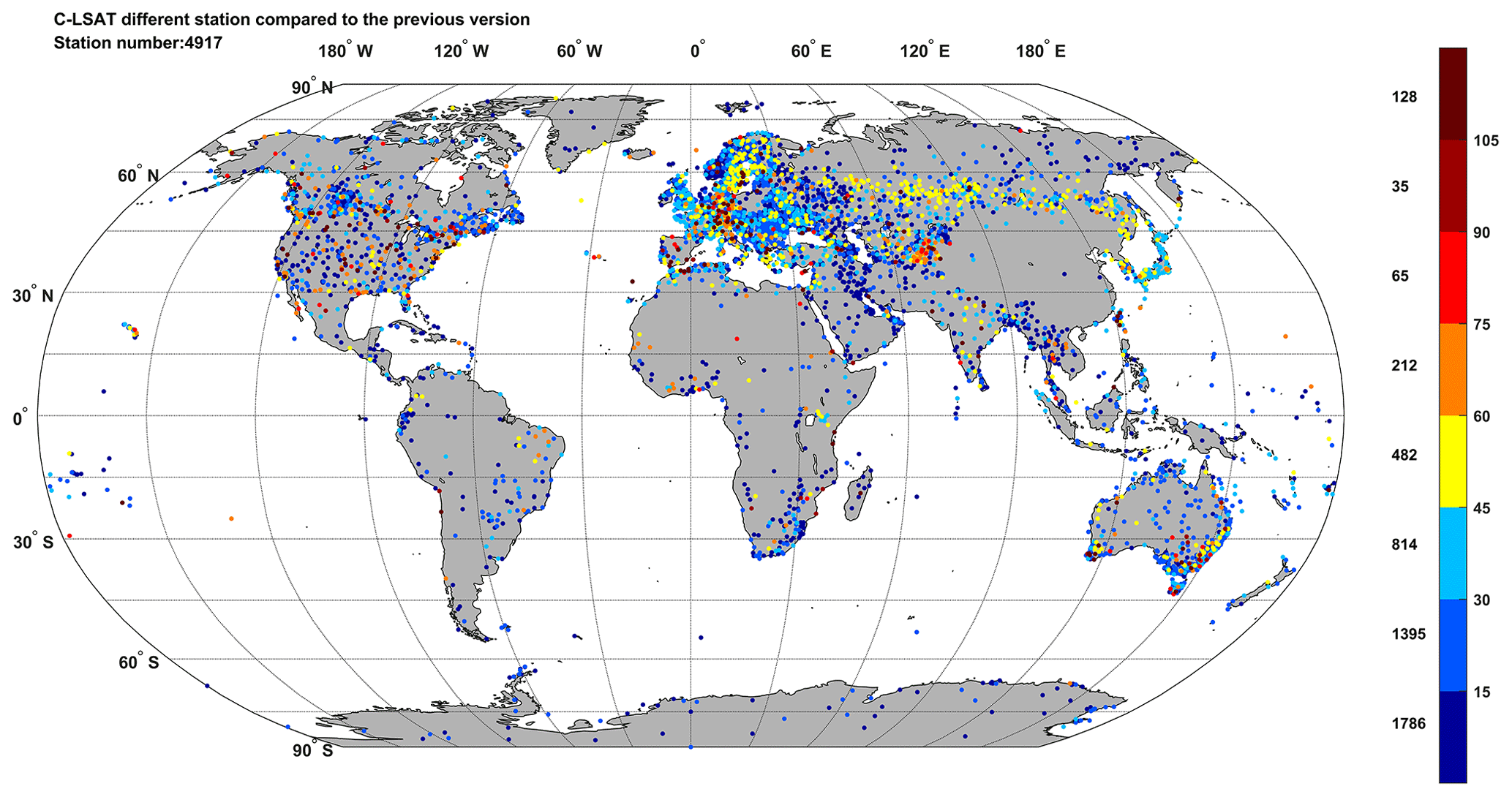
Figure 1Stations added in C-LSAT version 1.3 between 1900 and 2017. The number on the right side of the color bar indicated the length of time and the number on the left side is the station's number corresponding to a length of time.
The C-LSAT version 1.3 dataset is used in this study. Compared to C-LSAT version 1.0 from 1900 to 2014, version 1.3 is updated to December 2017. According to Xu et al. (2018), national, regional, and global datasets are ranked as higher, middle, and lower priorities, respectively. Based on the priority of the data resources, a total of 4917 high-priority stations were added, while a total of 1364 low-priority stations were deleted (replaced by higher-priority stations). Most of the newly added raw data (they are not the real “raw” data; most of them have been quality controlled) were obtained from the International Surface Temperature Initiative (ISTI) projects and have been homogenized through the same approach as Xu et al. (2018). The distribution of these extra 3553 stations is shown in Fig. 1. According to Xu et al. (2018), C-LSAT version 1.0 had some advantages over the existing global LSAT datasets in station number and spatial coverage. Thus, the current C-LSAT version 1.3 has more stations than the existing datasets in many regions over the global land surface. Figure 1 shows the extra stations compared to version 1.0, and Table 1 shows the comparison of the number of stations for different datasets, indicating an enhanced coverage and distribution/sampling of LSAT observations.
Table 1Comparison of the station number of the LSAT dataset during 1900–2017 (data length > 15 years).
2.1.2 Integration, QC, and homogenization of C-LSAT
All of the data sources collected were firstly merged into a single comprehensive dataset. The merge process was based on metadata matching and data equivalence criteria. Each candidate station was compared to all highest-priority (target) stations in two steps. In the first step, each candidate station was run through all the target stations and two metadata criteria were calculated for identifying matching stations: when (1) the distance of two separate stations (same name) falls within 5 km and the height difference falls within 50 m and (2) the Jaccard index (JI) (Jaccard, 1901; Xu et al., 2018) for two stations (different names) reaches 0.8, they pass the match test. In the second step, a data comparison was made between the same stations from different sources using the index of agreement (IA) (Willmott et al., 1985; Xu et al., 2018). If the IA reaches 0.8, the candidate station is merged with the target station. However, the lower-priority source is used where the higher-priority source is unavailable.
Similar to GHCN-V3 (Lawrimore et al., 2011), a three-step quality control (QC) process has been used for the merged dataset. QC 1 is the check for climate anomalies. Anomalies higher than 5 times the standard deviation of the monthly mean at each station are treated as missing; QC 2 is the check for spatial consistency. At a given time, or is considered an outlier and excluded (where Zi is the normalized (to the baseline period of 1961–1990) air temperature at the target station, Zij is the normalized air temperature at the neighboring stations (not exceeding 20) within 500 km from the target station, is the mean of normalized air temperature at the neighboring station, and σij is the standard deviation of normalized air temperature at the neighboring station). QC 3 is the check for internal consistency to ensure for the same month since internal inconsistency may arise when the station data have been integrated from different sources. The QC results show problematic data from 54 (QC1), 349 (QC2), and 1544 (QC3) station months and have been detected and treated as missing values. Although the proportion is relatively low (in total less than 0.02 %), the impact of the QC process on dataset products is significant.
At last, two steps were taken to ensure the homogeneity of the station time series: (1) the data series from the existing national homogenized datasets were directly integrated into C-LSAT without any change, which is approximately 50 % of the stations in C-LSAT. The benefit of including existing datasets is to improve the accuracy of regional climate change estimates by using several regional homogenized datasets developed by the corresponding NMHS (National Meteorological and Hydrological Services) or Climatic Data Centers. We believe that detailed metadata and expert knowledge will be helpful to generate better regional homogenized datasets, and the differences induced by using different homogenization methods are less important comparing with the differences in observing practices, instrumentation, and post-observation processing used by different nations/countries (Xu et al., 2018). (2) The inhomogeneities in the rest of the station series (Tm from about 6500 stations) were detected and adjusted with the penalized maximal t test method (Wang et al., 2007; Xu et al., 2018). The process is the same as that of Xu et al. (2018).
For comparison purposes, other LSAT datasets were collected from CRUTEM4 (https://www.metoffice.gov.uk/hadobs/crutem4/, last access: 1 August 2018) and GHCNm v3 (ftp://ftp.ncdc.noaa.gov/pub/data/ghcn/v3/, last access: 1 August 2018)1. All these datasets above were downloaded in August 2018. The following calculations are based on stations with a time length greater than 15 years between 1900 and 2017. From a global and hemispheric perspective, the C-LSAT version 1.3 dataset has more stations than the other datasets globally and in the Southern Hemisphere (SH) (Table 1). In addition, C-LSAT also has the largest number of stations for seven regions – Asia, Africa, Australia, South America, Europe, Antarctic, and the Arctic as defined in Xu et al. (2018).
2.2 Sea surface temperature data
In general, only in situ observational data were used when merging LSAT and SST for the commonly used global ST datasets. For example, HadCRUT4 and BE used HadSST3 (the median of 100 ensemble datasets); meanwhile NOAAGlobalTemp and GISTEMP used ERSSTv5. Both HadSST3 and ERSSTv5 datasets use only in situ data. Other datasets, such as COBE (Hirahara et al., 2014) and HadISST (Rayner et al., 2003), which uses both in situ and satellite data, were not used as a source in the merging of global ST data, although they are frequently used in SST studies. Therefore, the latter two SST datasets were used only for comparisons in this study.
3.1 Merging schemes
Generally in previous studies, the global ST dataset was merged using LSAT and SST datasets. Among all the existing global ST datasets (e.g., HadCRUT and NOAAGlobalTemp), the merging methods in combining the land and ocean datasets are basically very similar to each other (Morice et al., 2012; Vose et al., 2012). In this study, C-LSAT1.3 is merged with HadSST3 and ERSSTv5 (B. Huang et al., 2016, 2017, 2018) separately. The final merged global ST dataset will be selected based on the comparison of the quality of different merging schemes. These two SST datasets are reprocessed before the merging. The median of the 100-member ensemble datasets in HadSST3 was calculated for each grid box (Kennedy et al., 2011). The ERSSTv5 has a value of −1.8 ∘C in many grid boxes in the Arctic and Southern oceans, which refers to the area where the sea ice coverage is above 90 %. Therefore, some special treatment is needed for these grid boxes. If the anomalies are 0 ∘C and SSTs are −1.8 ∘C, then the value of −1.8 ∘C in ERSSTv5 will be replaced with missing values. The reference period for both HadSST3 and ERSSTv5 was taken as 1961–1990.
The two merging schemes are described as follows.
-
Merge1. C-LSAT1.3+HadSST3 (ensemble). Given the resolution of both datasets is , these two datasets were directly merged using the ratios of ocean and land surface areas in a specific grid box.
-
Merge2. C-LSAT1.3+ERSSTv5. Since the resolution of these two datasets is different, they were unified into the same resolution ( resolution), and then merged using the ratios of ocean and land areas.
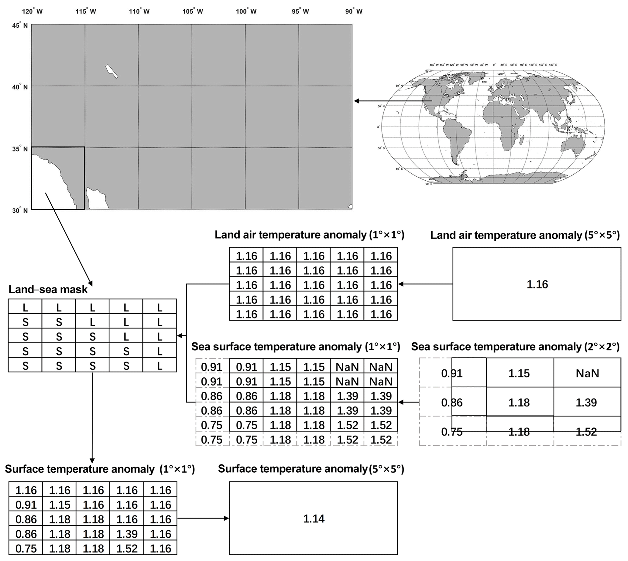
Figure 2Calculation method for temperature anomalies with a resolution of for the grid with ocean and land.
The merging process of C-LSAT1.3 and ERSST is described as follows (and in Fig. 2).
-
The anomalies were calculated in each grid box with respect to the base period 1961–1990 for C-LSAT and ERSSTv5.
-
For the ocean–land boundary part, the fraction of land and ocean areas is considered (see Fig. 2, taking January 2017 as an example). The detailed procedures are as follows.
- a.
Downscale the land (C-LSAT1.3) and ocean data to resolution. The resolution of the ocean data is , which is distributed in four grids of . The resolution of the land data is , which is distributed in 25 grids of .
- b.
Use the ocean–land mask file to differentiate all grids globally into land or ocean (download link: http://www.ncl.ucar.edu/Applications/Data/cdf/landsea.nc, last access: 8 August 2018). The ocean–land mask file is based on Rand's global elevation and depth data, and the resolution of the ocean–land mask is re-gridded to . The ocean–land mask file contains five types of markers: 0 for ocean, 1 for land, 2 for lakes, 3 for islands, and 4 for ice sheets. Marine data were used in parts of the ocean and ice sheets, and land data were used in parts of land, lakes, and small islands.
- c.
The ocean grid data and the land grid data were spliced by the ocean–land mask to obtain global ST grid data.
- d.
The averaged surface temperature anomaly (STA) in each grid was calculated as
- a.
3.2 Comparison of two merged schemes
Based on the methods above, C-LSAT1.3 grid data are merged with HadSST3 and ERSSTv5 data to form the C-LSAT+HadSST (Merge1) and C-LSAT+ERSST (Merge2) global ST datasets, respectively. In order to choose a better merging scheme in CMST, Merge1 and Merge2 were compared in two aspects: spatial coverage and representativeness in high latitudes.
3.2.1 Global coverage
The HadSST3 has not been interpolated, while the ERSSTv5 was interpolated by empirical orthogonal teleconnections (EOTs) (B. Huang et al., 2017). We do not distinguish the interpolated or non-interpolated boxes and compared these boxes with HadSST3 directly in the following sections because the interpolated ERSSTv5 data are meaningful and the final dataset contains all the interpolated values.
Table 2Mean, max, and min of monthly global coverage between 1900 and 2001 and between 2017 and 2012.
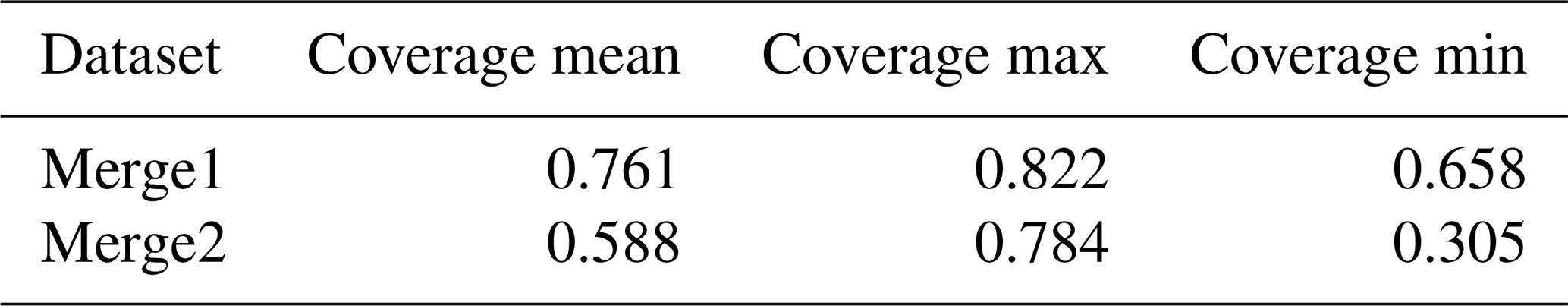
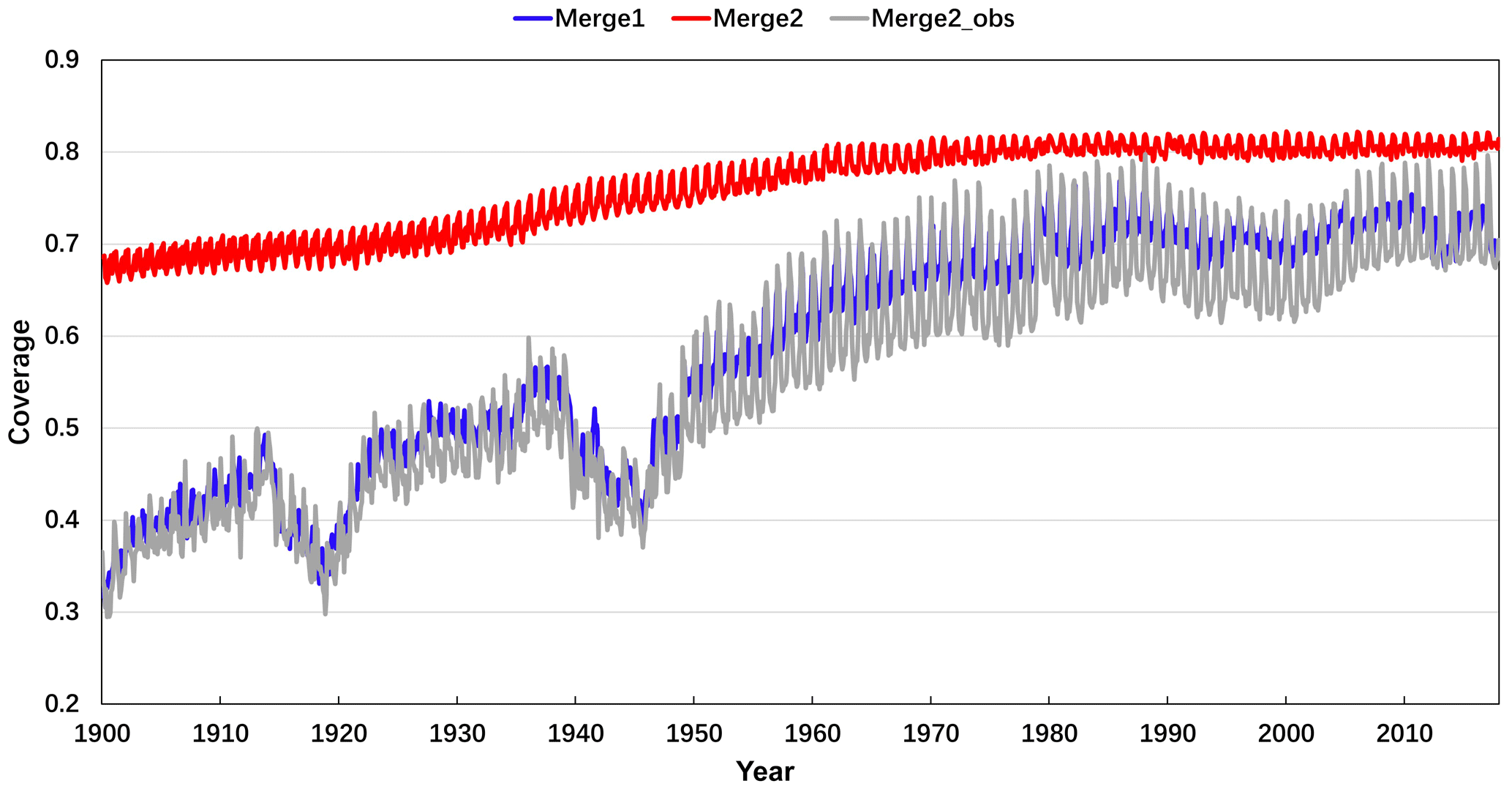
Figure 3Comparison of monthly global coverage of the two datasets from 1900 to 2017. The grey line is Merge2 but using the original data.
In Fig. 3, we found that the spatial coverage of Merge2 increases steadily with time from January 1900 to December 2017. In contrast, in the early and middle of the 20th century, the coverage of Merge1 changed dramatically with time, and became steady and close to Merge2 after the end of the 20th century. Note that if the ERSSTv5 original data were used (Merge2_obs), the coverage would be comparable with that of Merge1 for the whole period. In addition, Table 2 also shows the global coverage of Merge1 and Merge2. The maximum coverage was found in February 1988 for Merge1 and in January 2000 for Merge2. The minimum coverage was found in April 1900 for Merge 1 and June 1900 for Merge2. The mean coverage was calculated between 1900 and 2017. From Table 2, the Merge2 dataset has larger data coverage than Merge1 in coverage mean, coverage max, and coverage min. Although the difference between the two in coverage max is not very large, the difference in coverage means and coverage min between two merges is very large. This suggests that the coverage is mostly smaller in Merge1 than Merge2. Therefore, although the original data coverage of HadSST3 and ERSSTv5 is similar, but with the interpolation of EOTs, the latter increased its coverage greatly. Thus from the perspective of overall coverage, the dataset Merge2 is superior to Merge1 (Fig. 3).
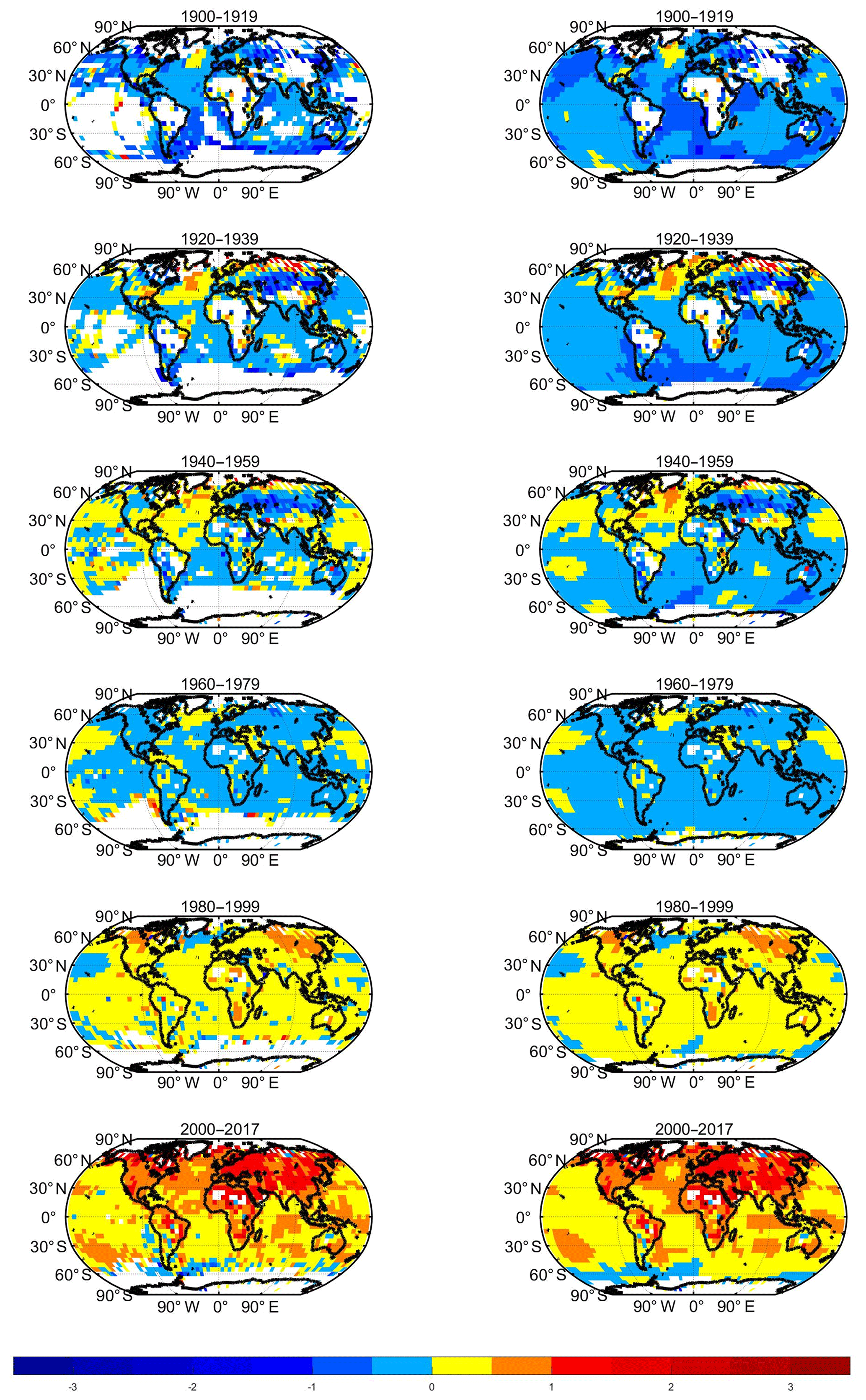
Figure 4Spatial distribution of 20-year average temperature anomalies between 1900 and 2017 in Merge1 (left) and Merge2 (right).
Furthermore, Fig. 4 shows the spatial coverage of the average temperature anomalies over 20 years for Merge1 and Merge2. The six panels in the left and right columns of Fig. 4 correspond to the 20-year mean temperature anomaly distribution over 1900–1919, 1920–1939, 1940–1959, 1960–1979, 1980–1999, and 2000–2017. In the early 20th century, it is clearly seen that Merge1 lacked a large range of data in the equatorial region, the western region of the SH, and the high-latitude zone of the SH. In the middle of the 20th century, Merge1 lacked so much data in the high latitudes of the SH. Merge1 continued to lack data at the high latitudes of the SH by the end of the 20th century. In contrast, Merge2 exhibited better data coverage globally, especially after the 2000s. This is due to the rapid increase in the number of observations from Argo5obs (Argo floats between 0 and 5 m depth) between 2000 and 2006. Since 2006, Argo5obs has maintained close to near-global coverage. In the high-latitude regions, the coverage of the Merge1 dataset is also smaller than that of Merge2, which may critically impact the assessment of climate over the Arctic. This is mainly because the spatial coverage of ICOADS R3.0 used in Merge2 is slightly higher than R2.5 used in Merge1, especially south of 60∘ S and north of 60∘ N (B. Huang et al., 2017). Therefore, the coverage of Merge1 is clearly lower than Merge2, particularly in the equatorial region and SH. Therefore, with respect to the spatial coverage of each period, Merge2 has a much better spatial coverage, especially in the early 20th century.
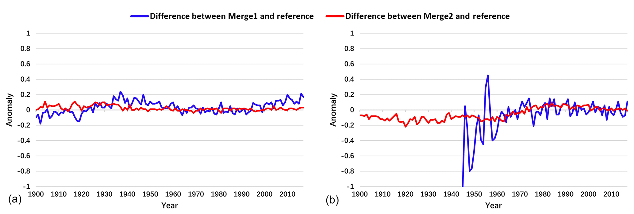
Figure 5Differences between the merged series and the reference series during 1900–2017 in (a) 90–60∘ N and (b) 60–90∘ S. The blue line shows the difference between Merge1 and the reference series, and the red line indicates the difference between Merge2 and the reference series.
3.2.2 Representativeness in high latitudes
To accurately compare the global and regional temperature changes between Merge1 and Merge2, COBE2, and HadISST1, which have satellite data integrated, were introduced. First, C-LSAT1.3 and COBE2, C-LSAT1.3, and HadISST1 datasets were merged in a similar way to form the Merge3 (C-LSAT+COBE) and Merge4 (C-LSAT+HadISST) datasets. Second, the monthly temperature anomalies of Merge1–4 to relatively the same baseline period (1961–1990) were calculated. The arithmetic mean of the four merged datasets was calculated for monthly temperature anomalies at each grid. As we know, each merging scheme might have uncertainties caused by different SST datasets, while the ensemble mean of all the merging datasets could have the least uncertainties. Therefore, the annual mean time series is calculated from the mean monthly temperature anomalies as a benchmark (reference series) for the two schemes.
From north to the south, the global ST is divided into five latitude zones: 90–60∘ N, 60–30∘ N, 30∘ N–30∘ S, 30–60∘ S, and 60–90∘ S. The reference series is subtracted from the Merge2 and Merge1 datasets to obtain a difference series for each region. The comparison between the two schemes indicated that the difference in midlatitude and low latitude is small (figure omitted). The difference is large in the high latitudes (Fig. 5). In 90–60∘ N, the difference between Merge2 and the reference series is steadily close to the 0 line during the period of 1900–2017, while the difference between Merge1 and the reference series is colder from the 1900s to 1920s and warmer from the 1930s to 1980s and also after the 1990s. In 60–90∘ S, the time series of Merge1 (1945) started later than Merge2 (1900), and the difference between Merge1 and the reference series (blue) is abnormally large from 1945 to the 1960s. The difference between Merge2 and the reference series (red) is still very small. The large difference in Fig. 5b may be associated with the small sampling size of the difference, or small coverage of Merge1, but Merge2 agrees well with what we expected.
The correlation coefficients between the time series of Merge1 and the reference series and between Merge2 and the reference sequence in each latitude zone were calculated. The results showed that the correlation coefficients between Merge1 (Merge2) and the reference series are similar for the globe, the SH, the Northern Hemisphere (NH), and the middle–low latitudes, which exceed 0.98. Compared with the reference series in the high-latitude zone, Merge2 shows much more consistence than Merge1. At 60–90∘ S, the correlation coefficient of Merge2 (0.90) is much larger than Merge1 (0.30). While for 90–60∘ N, the correlation coefficient of Merge2 (0.99) is slightly larger than Merge1 (0.97).
In summary, compared to Merge1, the Merge2 dataset is superior in terms of global coverage, spatial distribution, and the temporal change with the reference series. The possible reason is that the ocean data used by the ERSSTv5 dataset are the latest ICOADS R3.0 data, whereas the ocean data used by the HadSST3 dataset were obtained from ICOADS R2.5 (Woodruff et al., 2011). Also, the ERSSTv5 data incorporate more observations (such as Argo5obs). Based on the analysis above, Merge2 (C-LSAT1.3+ERSSTv5) was used as the final scheme in the later sections, which is named CMST (China Merged Surface Temperature).
4.1 Spatial coverage
Spatial coverage may differ among the following products due to the difference in spatial smoothing or interpolation method applied. HadCRUT4.6.0.0 is a non-interpolated observation dataset. NOAAGlobalTemp is first interpolated by EOTs in both LSAT and SST and then masked according to the actual observation availability. GISTEMP 250 km Smoothing (defined as GISTEMP1) is interpolated with a small scan radius. CMST is interpolated by EOTs in SST, but no interpolation is applied in LSAT.
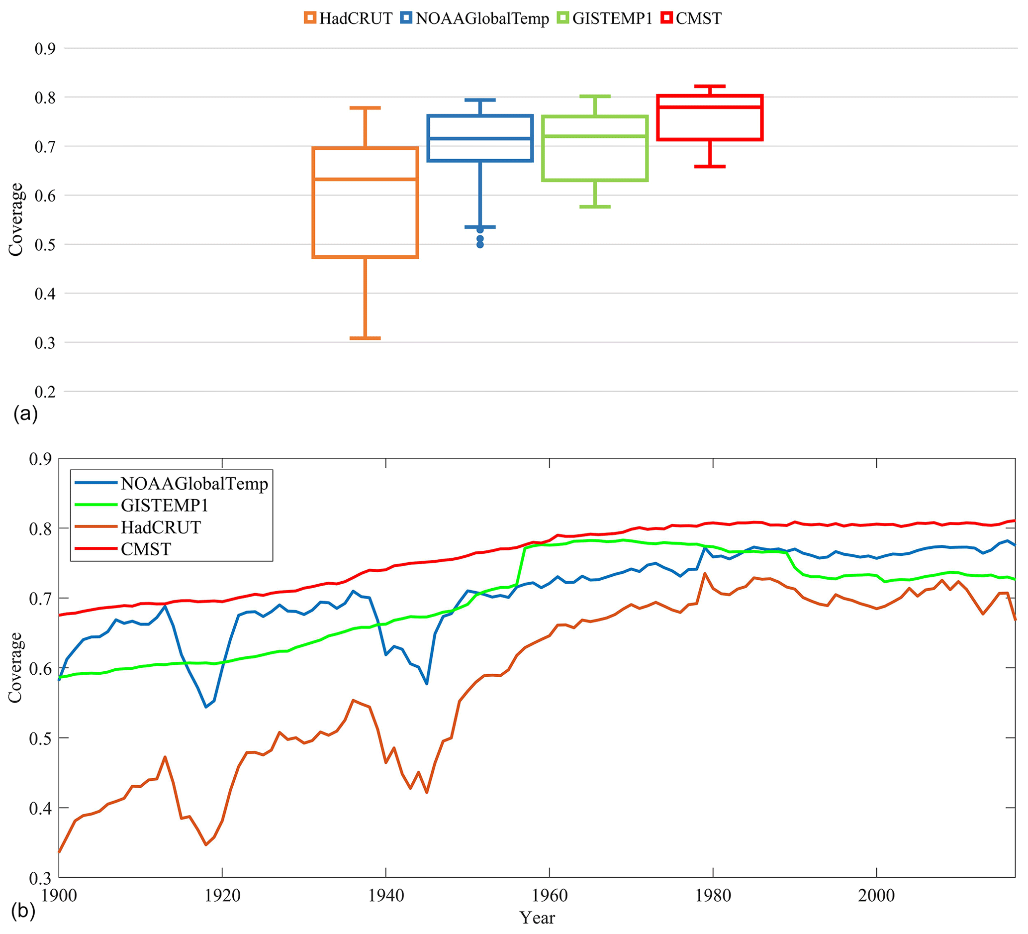
Figure 6Comparison of global ST dataset coverage between 1900 and 2017: (a) monthly coverage for all grid boxes; (b) annual average of coverage of monthly grid data.
First, the monthly coverage is calculated by the ratio of the areas between valid grid boxes and total grid boxes in HadCURT4, NOAAGlobalTemp, CMST, and GISTEMP1 (Fig. 6). Figure 6a shows that the area coverage in CMST is larger than that in other datasets with regards to coverage max, coverage min, and coverage mean. In particular the coverage min in CMST is much larger than that in the other datasets. Second, the monthly coverage is averaged to obtain the annual average. Figure 6 shows that the coverage of CMST is larger than that of the other three datasets at any time. Furthermore, the multi-year averaged coverage between 1900 and 2017 was calculated, which is 76 %, 58 %, 71 %, and 70 %, respectively, in CMST, HadCRUT4, NOAAGlobalTemp, and GISTEMP1. In other words, the coverage in CMST is not only much larger than that in the dataset without interpolation (such as HadCRUT4), but also larger than that in interpolated datasets (such as GISTEMP1 and NOAAGlobalTemp).
The reasons why the coverage of CMST is greater than that of the other datasets are as follows. The spatial coverage of land data (CRUTEM4) in HadCRUT4 is smaller than that of C-LSAT in CMST (Xu et al., 2018), and the spatial coverage of marine data (HasSST3) in HadCRUT4 is also smaller than ERSSTv5 in CMST. The higher coverage of marine data results from two aspects. (a) The ocean data (ERSSTv5) used by CMST have additional sources of Argo data and use ICOADS R3.0, which contains more ship and buoy data. (b) The ocean data of HadCRUT4 have not been interpolated, while the ocean data used by CMST were interpolated. The spatial coverage of the land dataset (GHCNm v3) in NOAAGlobalTemp is less than C-LSAT in CMST. The spatial coverage of the marine dataset (ERSSTv4) is also less than ERSSTv5, as ERSSTv5 incorporated new ICOADS data and added a decade of Argo float data. Additionally, GISTEMP1 has the same land dataset as NOAAGlobalTemp, its coverage is less than CMST, and its marine dataset is the same as CMST. Therefore, the spatial coverage of CMST is greater than GISTEMP1.
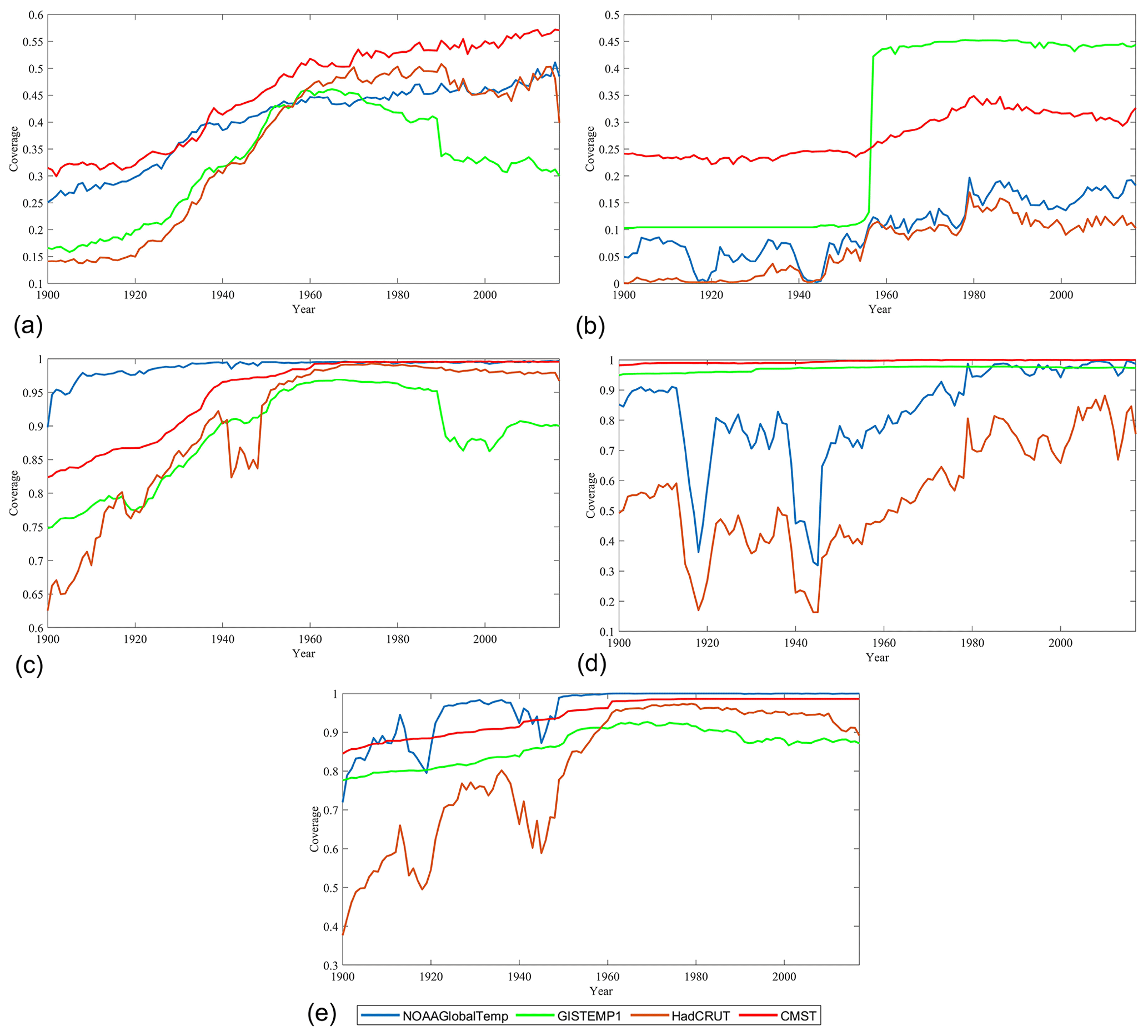
Figure 7Comparison of the annual averages of ST dataset coverage for each latitude zone between 1900 and 2017 in (a) 90–60∘ N, (b) 60–90∘ S, (c) 60–30∘ N, (d) 30–60∘ S, and (e) 30∘ N–30∘ S.
It should be noted that the data coverage of GISTEMP1 increases rapidly during the 1950s (Fig. 6b), which is mainly due to the rapid increase in the Antarctic (60–90∘ S; Fig. 7b). As in CMST, the station data of GISTEMP1 in Antarctic are mostly from SCAR (Hansen et al., 2010). The differences between these two datasets are that GISTEMP1 uses the baseline period from 1951 to 1980 while CMST uses the period of 1961 to 1990. Therefore, GISTEMP1 reserved more short-term stations within 1951–1980. Figure 6b also shows that HadCRUT4 and NOAAGlobalTemp have two minima in coverage around 1918 and 1943/1944. However, CMST and GISTEMP1 do not have these minima. We calculated the data coverage in five latitude zones (Fig. 7a–e) and noticed that the data coverage of HadCRUT4 and NOAAGlobalTemp has greater fluctuations in the latitude zones of 30∘ N–30∘ S and 30–60∘ S. Further analysis shows that the minimum value of 30–60∘ S coverage is the smallest, which has the greatest impact on the global coverage. Therefore, the minimum values of spatial coverage of HadCRUT4 and NOAAGlobalTemp are mainly due to the minimum coverage of 30–60∘ S. Since the 30–60∘ S latitude zone is dominated by oceans, the change of ST coverage in the 30–60∘ S latitude zone is likely related to the change of SST coverage. This result is consistent with what Vose et al. (2012) mentioned that the coverage of marine data decreased significantly during World War I and World War II. However, for CMST and GISTEMP, coverage is less affected during World War I and World War II because ERSSTv5 has been interpolated in many grid boxes with observations missing.
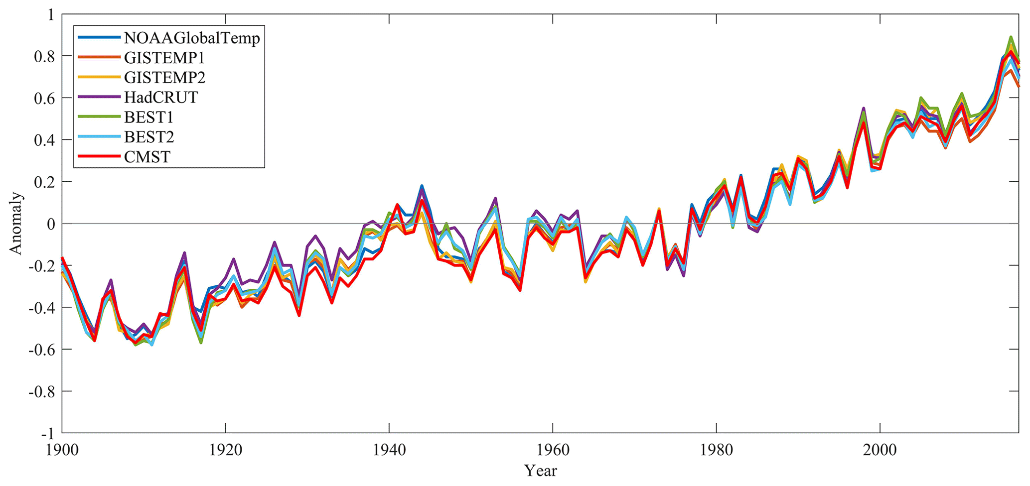
Figure 8Comparison of global mean ST anomalies series during 1900–2017 for different datasets (relative to 1961–1990).
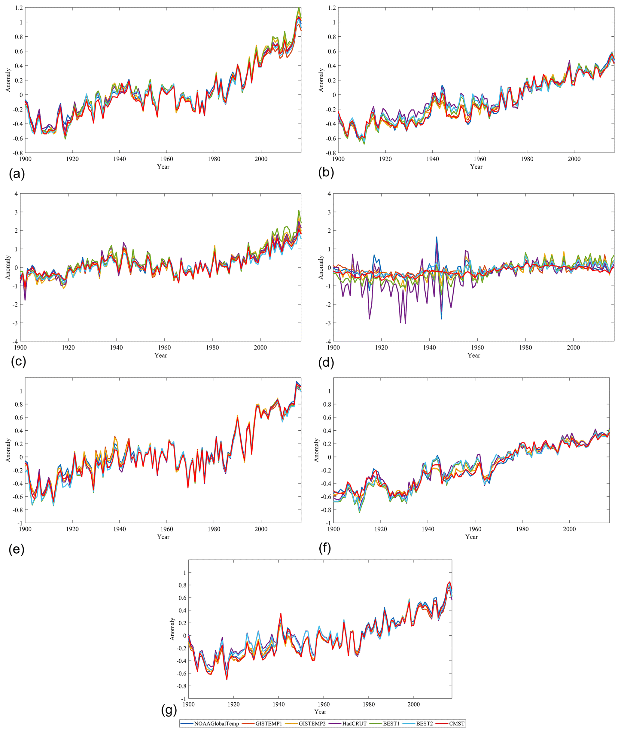
Figure 9Comparison of regional ST anomalies series during 1900–2017 in (a) NH, (b) SH, (c) 90–60∘ N, (d) 60–90∘ S, (e) 60–30∘ N, (f) 30–60∘ S, and (g) 30∘ N–30∘ S.
4.2 Inter-annual variations and trends
Figure 8 shows the area-weighted averaged time series of the global ST anomalies for the period 1990–2017 in seven datasets. Overall, the global ST changes in CMST and other datasets are similar over the period of 1900–2017. From the 1920s to 1970s, CMST is slightly lower, whereas HadCRUT4 is slightly higher than other datasets. The maximum differences between CMST and HadCRUT4 are in 1938 and 1948, and the difference in temperature anomalies within these two years is 0.18 ∘C. In 1938, the temperature anomalies are −0.17 and 0.01 ∘C in CMST and HadCRUT4, respectively. In 1948, the temperature anomalies are −0.20 and −0.02 ∘C in CMST and HadCRUT4, respectively. Further, the time series of ST anomalies in the seven datasets are also divided into the NH (a), the SH (b), and the five latitudinal zones 90–60∘ N (c), 60–30∘ N (e), 30∘ N–30∘ S (g), 30–60∘ S (f), and 60–90∘ S (h). Results clearly showed the time series of temperature anomalies in every dataset is highly consistent in the NH (Fig. 9a). At the low latitudes (Fig. 9e–g), the maximum ST of several datasets occurs in 2016, whereas the minimum occurs in different years. The minimum ST was found in 1917 for most of the datasets (GISTEMP1, GISTEMP2, BEST1, BEST2, HadCRUT4, and CMST), but it was found in 1908, 1909, and 1910 in NOAAGlobalTemp (Fig. 9a). In the midlatitude zone (Fig. 9e, f), the times with maximum ST in seven datasets are generally consistent. The maximum ST occurs in 2015 in 60–30∘ N and in 2017 in 30–60∘ S. The times with the minimum ST appear to be the same in seven datasets. The minimum ST was detected in 1912 in 60–30∘ N and in 1911 in 30–60∘ S. In the high latitudes of the NH, the maximum ST consistently occurs in 2016, and the minimum ST consistently occurred in 1902. In the high latitudes of the SH (Fig. 9d), the CMST is consistent with all the series derived from other datasets after 1960. There are many fewer stations and grid boxes in the Antarctic and higher latitudes; hence larger variances were found before 1960.
Table 3Regional ST trends for different latitude zones from 1900 to 2017 (degrees Celsius per decade).
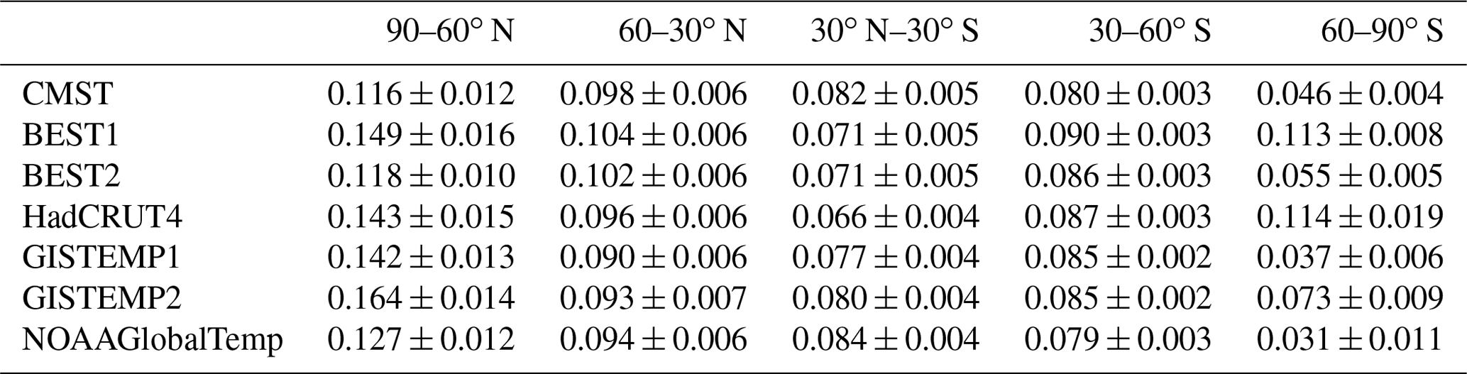
From Fig. 8, the temperature anomalies showed a clear warming trend from 1900 to 2017. For CMST, the highest temperature anomaly is 0.82 ∘C in 2016. There is a significant warming trend from the 1910s to 1940s and the 1960s to 2017. In contrast, there is a cooling trend from the 1940s to 1960s. The changes were highly consistent with the other datasets and are related to the changes of El Niño and La Niña events, volcanic eruptions, sea ice cover, and other factors (Simmons et al., 2017). Li et al. (2019b) showed that the ST warming trend during 1998–2012 derived from CMST was slightly increased compared with the existing datasets and is statistically significant. It becomes closer among the newly developed global observational data (CMST), remote sensed/Buoy network infilled dataset, and adjusted reanalysis data (Cowtan and Way, 2014; J. Huang et al., 2017; Simmons et al., 2017). The temperature trends for the period of 1900–2017 in different latitudinal belts were compared among these datasets: GISTEMP 250 km Smoothing (defined as GISTEMP1), GISTEMP 1200 km Smoothing (defined as GISTEMP2), BEST with air temperatures over sea ice (defined as BEST1), BEST with water temperatures below sea ice (defined as BEST2), NOAAGlobalTemp, HadCRUT4, and CMST (Table 3). The ST trend in the NH high latitudes is the largest (0.116±0.012 ∘C per decade), lower in the midlatitudes of the NH (0.098±0.006 ∘C per decade), the midlatitudes of the SH (0.080±0.003 ∘C per decade), and the low latitudes (0.082±0.005 ∘C per decade), and the lowest temperature trend is found in the high latitudes of the SH (0.046±0.004 ∘C per decade) in CMST. The ST trends with the largest difference among different datasets occurred in the high latitudes (from 0.031±0.011 ∘C per decade in NOAAGlobalTemp to 0.114±0.019 ∘C per decade in HadCRUT4), which shows the larger uncertainties in southern polar regions. In the high latitudes of the NH, the highest ST trend was found in GISTEMP2 (0.164±0.014 ∘C per decade) and BEST1 (0.149±0.016 ∘C per decade) and the lowest in CMST (0.116±0.012 ∘C per decade), while the former two are believed to be overestimated due to the use of air temperature over sea ice in polar regions. The differences are lower in the middle and low latitudes; the trends in CMST are all between the maximum and the minimum in different datasets.
The datasets used in CMST were derived from published data by NHMS (China, Russia, the USA, Canada, Australia, some Asian countries, etc.) or climate data research institutions (UK CRU, NOAA NCEI). Part of the data are exchanged between some countries or regions, and therefore are conditionally available to the public. Details of the data sources are as follows. C-LSAT 1.3 in gridded form with a resolution of developed by SUN Yat-Sen University (SYSU) and China Meteorological Administration is available on the Climate Explorer website of the Royal Netherlands Meteorological Institute (KNMI) (http://climexp.knmi.nl/select.cgi?id=someone@somewhere&field=clsat_tavg, last access: 12 December 2017). ERSST.v5 is from NOAA NCEI at https://www.ncdc.noaa.gov/data-access/marineocean-data/extended-reconstructed-sea-surface-temperature-ersst-v5 (last access: 11 August 2018). The China Merged Surface Temperature Data (CMST) dataset developed by SYSU is currently publicly available on the Climate Explorer website of the Royal Netherlands Meteorological Institute (KNMI) (http://climexp.knmi.nl/select.cgi?id=someone@somewhere&field=cmst, last access: 11 August 2018). With the digital object identifiers (DOIs) (https://doi.org/10.1594/PANGAEA.901295) issued for the datasets (Li, 2019a), we hope to have provided a repository of a new global ST analysis covering the past 120 years from now to the year 1900 for the scientific user community as well as the public.
A new global ST dataset of CMST (China Merged Surface Temperature) has been developed based on the LSAT dataset (C-LSAT1.3) and SST dataset (ERSSTv5). This dataset was completed by the cooperation between SUN Yat-sen University (SYSU), China Meteorological Administration (CMA), and the United States NOAA NCEI. In CMST, we found the following.
-
The spatial coverage is larger when C-LSAT1.3 and ERSSTv5 are merged than when merging C-LSAT1.3 with HadSST3, particularly in the polar regions. In addition, the former (merging C-LSAT1.3 with ERSSTv5, named CMST) is also superior in terms of spatial distribution and temporal change with the reference series (derived from the average of merged C-LSAT1.3 and four SST datasets).
-
The LSAT in CMST used the high-quality C-LSAT1.3. More than 4900 stations were added to the previous version of C-LSAT1.0 (Xu et al., 2018), which has further increased the data coverage. The newly added stations are mainly from the ISTI dataset. The SST in CMST uses ERSSTv5 with the ocean data from the latest ICOADS R3.0 and incorporates multiple types of observations. Compared with other existing global ST datasets, the CMST increases the overall coverage over global land and ocean surface.
-
The time series in CMST globally and in the middle–low latitudes are consistent with the other merged datasets for both inter-annual and inter-decadal timescales. In the high-latitude zones of the NH and SH where the differences of temperature trends are usually larger, the trend of CMST represents the major long-term climate changes. Therefore, the CMST temperature trend from 1900 to 2017 is overall consistent with other datasets and proved to be a new useful tool in global climate change studies.
All co-authors participated in the data collection, data analysis, and development of the dataset. QL was primarily responsible for the writing of the paper and assembly of the archival database. QL, XY, and BH conceived of the study design with input from all co-authors. All authors contributed to the writing of the paper.
The authors declare that they have no conflict of interest.
We thank the many people and/or institutions who contributed to the establishment of this dataset.
This research has been supported by the National Key R&D Program of China (grant nos. 2017YFC1502301 and 2018YFC1507705), the Natural Science Foundation of China (grant no. 41975105), and the China Postdoctoral Science Foundation (grant no. 2018M640848).
This paper was edited by Scott Stevens and reviewed by two anonymous referees.
Anderson, B. T.: Near-term increase in frequency of seasonal temperature extremes prior to the 2∘ global warming target, Clim. Change, 108, 581–589, https://doi.org/10.1007/s10584-011-0196-4, 2011.
Church, J. A., Clark, P. U., Cazenave, A., Gregory, J. M., Jevrejeva, S., Levermann, A., and Payne, A. J.: Climate change 2013: the physical science basis. Contribution of Working Group I to the Fifth Assessment Report of the Intergovernmental Panel on Climate Change, Sea level change, 1137–1216, 2013.
Cowtan, K. and Way, R. G.: Coverage bias in the HadCRUT4 temperature series and its impact on recent temperature trends, Q. J. Roy. Meteor. Soc., 140, 1935–1944, https://doi.org/10.1002/qj.2297, 2014.
Freeman, E., Woodruff, S. D., Worley, S. J., Lubker, S. J., Kent, E. C., Angel, W. E., Berry, D. I., Brohan P., Eastman, R., Gates, L., Gloeden, W., Ji, Z., Lawrimore, J., Rayner, N. A., Rosenhagen, G. S., and Shawn R.: ICOADS Release 3.0: a major update to the historical marine climate record, Int. J. Climatol., 37, 2211–2232, https://doi.org/10.1002/joc.4775, 2017.
Hansen, J., Ruedy, R., Sato, M., and Lo, K.: Global surface temperature change, Rev. Geophys., 48, RG4004, https://doi.org/10.1029/2010RG000345, 2010.
Hirahara, S., Ishii, M., and Fukuda, Y.: Centennial-scale sea surface temperature analysis and its uncertainty, J. Climate, 30, 57–75, https://doi.org/10.1175/JCLI-D-12-00837.1, 2014.
Huang, B., Banzon, V. F., Freeman, E., Lawrimore, J., Liu, W., Peterson, T. C., Smith, T. M., Thorne, P. W., Woodruff, S. D., and Zhang, H. M.: Extended Reconstructed Sea Surface Temperature Version 4 (ERSST.v4), Part I. Upgrades and intercomparisons, J. Climate, 28, 911–930, https://doi.org/10.1175/JCLI-D-14-00006.1, 2015.
Huang, B., Thorne, P. W., Smith, T. M., Liu, W., Lawrimore, J., Banzon, V. F., Zhang, H. M., Peterson, T. C., and Menne, M.: Further exploring and quantifying uncertainties for extended reconstructed sea surface temperature (ERSST) version 4 (v4), J. Climate, 29, 3119–3142, https://doi.org/10.1175/JCLI-D-15-0430.1, 2016.
Huang, B., Thorne, P. W., Banzon, V. F., Boyer, T., Chepurin, G., Lawrimore, J. H., Menne M. J., Smith, T. M., Vose R. S., and Zhang, H. M.: Extended reconstructed sea surface temperature, version 5 (ERSSTv5): upgrades, validations, and intercomparisons, J. Climate, 30, 8179–8205, https://doi.org/10.1175/JCLI-D-16-0836.1, 2017.
Huang, B., Angel, W., Boyer, T., Cheng, L., Chepurin, G., Freeman, E., Liu, C., and Zhang, H. M.: Evaluating SST analyse s with independent ocean profile observations, J. Climate, 31, 5015–5030, https://doi.org/10.1175/JCLI-D-17-0824.1, 2018.
Huang, J., Zhang, X., Zhang, Q., Lin, Y., Hao, M., Luo, Y., Zhao, Z., Yao, Y., Chen, X., Wang, L., Nie, S., Yin, Y., Xu, Y., and Zhang, J.: Recently amplified arctic warming has contributed to a continual global warming trend, Nat. Clim. Change, 7, 875–879, https://doi.org/10.1038/s41558-017-0009-5, 2017.
IPCC: Climate Change 2013: The Physical Science Basis, in: Contribution of Working Group I to the Fifth Assessment Report of the Intergovernmental Panel on Climate Change, edited by: Stocker, T. F., Qin, D., Plattner, G.-K., Tignor, M., Allen, S. K., Boschung, J., Nauels, A., Xia, Y., Bex, V., and Midgley, P. M., Cambridge University Press, Cambridge, UK and New York, NY, 1535 pp., 2013.
Jaccard, P.: Etude comparative de la distribution florale dans une portion des Alpes et des Jura, B. Soc. Vaudoise Sci. Natur., 37, 547–579, 1901.
Jones, P. D.: The reliability of global and hemispheric surface temperature records, Adv. Atmos. Sci., 33, 269–282, https://doi.org/10.1007/s00376-015-5194-4, 2016.
Jones, P. D. and Moberg, A.: Hemispheric and large-scale surface air temperature variations: An extensive revision and an update to 2001, J. Climate, 16, 206–223, https://doi.org/10.1175/1520-0442(2003)016<0206:HALSSA>2.0.CO;2, 2003.
Jones, P. D., Lister, D. H., Osborn, T. J., Harpham, C., Salmon, M., and Morice, C. P.: Hemispheric and large-scale land-surface air temperature variations: An extensive revision and an update to 2010, J. Geophys. Res.-Atmos., 117, D05127, https://doi.org/10.1029/2011JD017139, 2012.
Kennedy, J. J., Rayner, N. A., Smith, R. O., Parker, D. E., and Saunby, M.: Reassessing biases and other uncertainties in sea surface temperature observations measured in situ since 1850: 2. Biases and homogenization, J. Geophys. Res.-Atmos., 116, D14104, https://doi.org/10.1029/2010JD015220, 2011.
Lawrimore, J. H., Menne, M. J., Gleason, B. E., Williams, C. N., Wuertz, D. B., Vose, R. S., and Rennie, J.: An overview of the Global Historical Climatology Network monthly mean temperature data set, version 3, J. Geophys. Res.-Atmos., 116, D19121, https://doi.org/10.1029/2011JD016187, 2011.
Li, Q.: China Merged Surface Temperature, dataset, SUN Yat-sen University, https://doi.org/10.1594/PANGAEA.901295, 2019a.
Li, Q.: China Merged Surface Temperature (CMST) (version1) [Data Set], KNMI, available at: http://climexp.knmi.nl/select.cgi?id=someone@somewhere&field=cmst, last access: 27 October 2019b.
Li, Q.: China Land Surface Air Temperature (C-LSAT) (version1.3) [Data Set], KNMI, available at: http://climexp.knmi.nl/select.cgi?id=someone@somewhere&field=clsat_tavg, last access: 27 October 2019c.
Li, Q., Zhang, H., Liu, X., Chen, J., Li, W., and Jones, P. D.: A mainland China homogenized historical temperature dataset of 1951–2004, B. Am. Meteor. Soc., 90, 1062–1065, https://doi.org/10.1175/2009BAMS2736.1, 2009.
Li, Q., Zhang, L., Xu, W., Zhou, T., Wang, J., Zhai, P., and Jones, P. D.: Comparisons of time series of annual mean surface air temperature for china since the 1900s: Observations, model simulations, and extended reanalysis, B. Am. Meteor. Soc., 98, 699–711, https://doi.org/10.1175/BAMS-D-16-0092.1, 2017.
Li, Q., Dong, W., and Jones, P.: Continental Scale Surface Air Temperature Variations: Experience Derived from Chinese Region, Earth-Sci. Rev., accepted, 2019a.
Li, Q., Yun, X., Huang, B., Dong, W., Wang, X. L., Zhai, P., and Jones, P. D.: An update evaluation on the global surface temperature change trends since the start of the 20th century, Clim. Dynam., in review, 2019b.
Menne, M. J., Williams, C. N., Gleason, B. E., Rennie, J. J., and Lawrimore, J. H.: The Global Historical Climatology Network Monthly Temperature Dataset, Version 4, J. Climate, 31, 9835–9854, https://doi.org/10.1175/JCLI-D-18-0094.1, 2018.
Morice, C. P., Kennedy, J. J., Rayner, N. A., and Jones, P. D.: Quantifying uncertainties in global and regional temperature change using an ensemble of observational estimates: The HadCRUT4 data set, J. Geophys. Res.-Atmos., 117, D08101, https://doi.org/10.1029/2011JD017187, 2012.
Osborn, T. J. and Jones, P. D.: The CRUTEM4 land-surface air temperature data set: construction, previous versions and dissemination via Google Earth, Earth Syst. Sci. Data, 6, 61–68, https://doi.org/10.5194/essd-6-61-2014, 2014.
Peterson, T. C. and Vose, R. S.: An overview of the Global Historical Climatology Network temperature database, B. Am. Meteor. Soc., 78, 2837–2850, https://doi.org/10.1175/1520-0477(1997)078<2837:AOOTGH>2.0.CO;2, 1997.
Rayner, N. A. A., Parker, D. E., Horton, E. B., Folland, C. K., Alexander, L. V., Rowell, D. P., Kent, E. C., and Kaplan, A.: Global analyses of sea surface temperature, sea ice, and night marine air temperature since the late nineteenth century, J. Geophys. Res.-Atmos., 108, 4407, https://doi.org/10.1029/2002JD002670, 2003.
Rohde, R., Muller, R. A., Jacobsen, R., Muller, E., Perlmutter, S., Rosenfeld, A., Wurtele, J., Groom, D., and Wickham, C.: A new estimate of the average Earth surface land temperature spanning 1753 to 2011, Geoinfor. Geostat. Overview, Sci. Technol., 1, 10000101, https://doi.org/10.4172/2327-4581.1000101, 2013.
Simmons, A. J., Berrisford, P., Dee, D. P., Hersbach, H., Hirahara, S., and Thépaut, J. N.: A reassessment of temperature variations and trends from global reanalyses and monthly surface climatological datasets, Q. J. Roy. Meteor. Soc., 143, 101–119, 2017.
Thorne, P. W., Willett, K. M., Allan, R. J., Bojinski, S., Christy, J. R., Fox, N., Gilbert, S., Jolliffe, I., Kennedy, J. J., Kent, E., Tank, A. K., Lawrimore, J., Parker, D, E., Rayner, N., Simmons, A., Song, L., Stott, P. A., and Trewin, B.: Guiding the creation of a comprehensive surface temperature resource for twenty-first-century climate science, B. Am. Meteor. Soc., 92, ES40–ES47, https://doi.org/10.1175/2011BAMS3124.1, 2011.
Trewin, B.: A daily homogenized temperature data set for Australia, Int. J. Climatol., 33, 1510–1529, 2013.
Turner, J., Colwell, S. R., Marshall, G. J., Lachlan-Cope, T. A., Carleton, A. M., Jones, P. D., Lagun, V., Reid, P. A., and Iagovkina, S.: The SCAR READER project: Toward a high-quality database of mean Antarctic meteorological observations, J. Climate, 17, 2890–2898, https://doi.org/10.1175/1520-0442(2004)017<2890:TSRPTA>2.0.CO;2, 2004.
Vincent, L. A., Wang, X. L., Milewska, E. J., Wan, H., Yang, F., and Swail, V.: A second generation of homogenized Canadian monthly surface air temperature for climate trend analysis, J. Geophys. Res.-Atmos., 117, D18110, https://doi.org/10.1029/2012JD017859, 2012.
Vose, R. S., Arndt, D., Banzon, V. F., Easterling, D. R., Gleason, B., Huang, B., Kearns, E., Lawrimore, J. H., Menne, M. J., and Peterson, T. C.: NOAA's merged land–ocean surface temperature analysis, B. Am. Meteor. Soc., 93, 1677–1685, https://doi.org/10.1175/BAMS-D-11-00241.1, 2012.
Wang, X. L., Wen, Q. H., and Wu, Y.: Penalized maximal t test for detecting undocumented mean change in climate data series, J. Appl. Meteorol. Clim., 46, 916–931, https://doi.org/10.1175/JAM2504.1, 2007.
Willmott, C. J., Ackleson, S. G., Davis, R. E., Feddema, J. J., Klink, K. M., Legates, D. R., O'Donnell, J., and Rowe, C. M.: Statistics for the evaluation and comparisons of models, J. Geophys. Res., 90, 8995–9005, https://doi.org/10.1029/JC090iC05p08995, 1985.
Woodruff, S. D., Worley, S. J., Lubker, S. J., Ji, Z., Eric Freeman, J., Berry, D. I., Brohan, P., Kent, E. C., Reynolds, R. W., Smith, S. R., and Wilkinson, C.: ICOADS Release 2.5: extensions and enhancements to the surface marine meteorological archive, Int. J. Climatol., 31, 951–967, https://doi.org/10.1002/joc.2103, 2011.
Xu, C., Wang, J, Hu, M., and Li, Q.: Interpolation of missing temperature data at meteorological stations using P-BSHADE, J. Climate, 26, 7452–7463, https://doi.org/10.1175/JCLI-D-12-00633.1, 2013.
Xu, W., Li, Q., Jones, P., Wang, X. L., Trewin, B., Yang, S., Zhu C., Zhai P., Wang J., Vincent L., Dai, A., Gao, Y., and Ding, Y.: A new integrated and homogenized global monthly land surface air temperature dataset for the period since 1900, Clim. Dynam., 50, 2513–2536, https://doi.org/10.1007/s00382-017-3755-1, 2018.
Despite careful efforts we could not extract reliable information from BEST. Thus the comparison with BEST has been deleted according to the reviewer's suggestion.