the Creative Commons Attribution 4.0 License.
the Creative Commons Attribution 4.0 License.
 | 23 May 2018
ReOBS: a new approach to synthesize long-term multi-variable dataset and application to the SIRTA supersite
Marjolaine Chiriaco
Jean-Charles Dupont
Sophie Bastin
Jordi Badosa
Julio Lopez
Martial Haeffelin
Helene Chepfer
Rodrigo Guzman
A scientific approach is presented to aggregate and harmonize a set of 60 geophysical variables at hourly timescale over a decade, and to allow multiannual and multi-variable studies combining atmospheric dynamics and thermodynamics, radiation, clouds and aerosols from ground-based observations. Many datasets from ground-based observations are currently in use worldwide. They are very valuable because they contain complete and precise information due to their spatio-temporal co-localization over more than a decade. These datasets, in particular the synergy between different type of observations, are under-used because of their complexity and diversity due to calibration, quality control, treatment, format, temporal averaging, metadata, etc. Two main results are presented in this article: (1) a set of methods available for the community to robustly and reliably process ground-based data at an hourly timescale over a decade is described and (2) a single netCDF file is provided based on the SIRTA supersite observations. This file contains approximately 60 geophysical variables (atmospheric and in ground) hourly averaged over a decade for the longest variables. The netCDF file is available and easy to use for the community. In this article, observations are “re-analyzed”. The prefix “re” refers to six main steps: calibration, quality control, treatment, hourly averaging, homogenization of the formats and associated metadata, as well as expertise on more than a decade of observations. In contrast, previous studies (i) took only some of these six steps into account for each variable, (ii) did not aggregate all variables together in a single file and (iii) did not offer an hourly resolution for about 60 variables over a decade (for the longest variables). The approach described in this article can be applied to different supersites and to additional variables. The main implication of this work is that complex atmospheric observations are made readily available for scientists who are non-experts in measurements. The dataset from SIRTA observations can be downloaded at http://sirta.ipsl.fr/reobs.html (last access: April 2017) (Downloads tab, no password required) under https://doi.org/10.14768/4F63BAD4-E6AF-4101-AD5A-61D4A34620DE.
- Article
(10379 KB) - Full-text XML
- BibTeX
- EndNote


The Intergovernmental Panel on Climate Change (IPCC) simulations show a large spread between models when predicting future climate at a global scale, but also when representing the observed current climate. These model uncertainties are larger at the regional scale and at short timescales (e.g., seasonal scale). These scales are, however, key for the impact assessment. For example, models do not reproduce observed magnitudes of interannual and seasonal variability and extremes in temperature and precipitation (Terray and Boé, 2013). Hawkins and Sutton (2009) also show that climate's natural variability is the main source of uncertainty to predict regional climate evolution at the timescale of 10–20 years (compared to the selected scenario or model). Observations of the atmosphere must be considered in order to improve both our knowledge of the processes that create this temporal variability and the simulation uncertainties. These observations must describe atmospheric processes that involve a large number of variables in the atmospheric columns and in the ground, and at various spatial and temporal scales.
Multiannual and multi-variable datasets are therefore necessary. Many of these datasets from ground-based observations have a significant scientific value because they contain complete and precise information on one or several decades, due to their spatio-temporal co-localization. Supersite observatories such as the Site Instrumental de Recherche par Télédétection Atmosphérqiue (SIRTA, Haeffelin et al., 2005) or the different Atmospheric Radiation Measurements (ARM, Ackerman et al., 2003) are among these sets of observations. But they are under-used, in particular the observed synergy aspects, because of their complexity and diversity in terms of calibration procedures, quality control, data treatment, file format, temporal representativeness, metadata etc., and because of the weak magnitude of the signals to be highlighted (e.g., trend versus natural variability), and also because of the complex connections between local-scale processes and climatic-scale anomalies (e.g., links between ground–boundary-layer–atmosphere processes and heat waves; as in Chiriaco et al., 2014).
An important homogenization work was needed for these observations. Homogenization has been performed for ARM observatories leading to the ARMBE (ARM Best Estimate) data product (Xie et al., 2010), which is the “ARM data streams specifically tailored to climate modelers for use in the evaluation of global climate models. They contain a best estimate of several cloud, radiation and atmospheric quantities. The ARMBE dataset was created to showcase all the flagship products of ARM” (from https://www.arm.gov/capabilities/vaps/armbe, last access: April 2017). A specificity of ARMBE products is that all variables are gathered in only two files: ARMBEATM (ATM for atmosphere) for many atmospheric state profiles and surface quantities, and ARMBECLDRAD (CLDRAD for cloud and radiation) that contains a best estimate of several selected ARM and satellite-measured cloud- and radiation-relevant quantities.
In this article, additional steps are applied to the observations and precisely described in order to understand how the observations are “re-analyzed”. This method is called ReOBS. The prefix “Re” refers to six main steps on more than a decade of observations: calibration, quality control, algorithmic treatment, hourly averaging, homogenization of the data formats and associated metadata, as well as scientist expertise. In contrast, previous studies (i) only take into account some of these six steps for each variable, (ii) do not aggregate together all variables in a single file and (iii) do not offer an hourly resolution for about 60 variables over a decade (for the oldest variables).
The ReOBS method was initially inspired by the ARMBE project and has been developed at SIRTA (located 20 km southwest of Paris, France). The SIRTA observatory has been collecting data for 15 years from active and passive remote sensing, in situ measurements at the surface, in the ground and in the planetary boundary layer (PBL). Early versions of the SIRTA ReOBS dataset have already been used in scientific studies that required the multi-variables and multi-temporal scales available in the SIRTA-ReOBS dataset (Cheruy et al., 2012; Chiriaco et al., 2014; Pal and Haeffelin, 2015, Bastin et al., 2016; Dione et al., 2017). The ReOBS method has also been tested for other supersites for some variables (classical meteorology, radiative fluxes, heat fluxes): Cabauw (in the Netherlands) and Chilbolton (in England) supersites in the framework of the EUCLIPSE European project (European Union Cloud Intercomparison, Process Study and Evaluation project), CO-PDD (Cézeaux – Opme – Puy De Dôme at Clermont Ferrand in France) and P2OA (Plateforme Pyrénéenne d'Observations Atmosphériques at Lannemezan in France) in Dione et al. (2016).
The objective of the current paper is to present a scientific approach (ReOBS) to aggregate and harmonize about 60 geophysical variables at hourly timescale over at least a decade, and to study atmospheric dynamics and thermodynamics, radiation, clouds and aerosols from ground-based observations. This paper presents two main results: (1) a set of methods available for the community to process ground-based data robustly and reliably at an hourly timescale over at least a decade and (2) provision of a single netCDF file containing about 60 substantial geophysical variables hourly averaged over 15 years for the oldest ones, and easily usable for the community.
The SIRTA observations used for applying the ReOBS method are described in Sect. 2. The method used for ReOBS is then detailed in Sect. 3. Section 4 presents the contents of the SIRTA-ReOBS file and its major strengths: the vertical profiles, the multi-temporal scales and the multi-parameter specificity. Discussion and conclusions are presented in Sect. 5.
2.1 SIRTA observatory
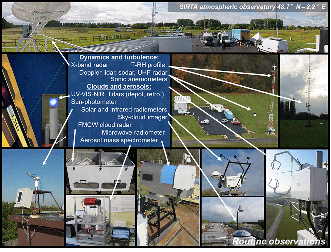
SIRTA is a French national observatory dedicated to the monitoring of tropospheric clouds and aerosols, the dynamics and thermodynamics of the boundary layer, and the turbulent and organized transport of water and energy near the surface. The SIRTA observatory is a mid-latitude site (48.71∘ N, 2.2∘ E) located in a semi-urban area on the Saclay plateau 20 km southwest of Paris, and hosts active and passive remote-sensing instruments since 2002 (Haeffelin et al., 2005). The SIRTA missions are (1) to monitor continuously and in the long-term the atmospheric column using a core ensemble of instruments; (2) to coordinate field campaigns in order to address specific scientific questions, such as processes related to water vapor and clouds, the ultraviolet radiation, or the aerosol physics and chemistry; and (3) to provide teaching resources and to host experimental training activities.
Figure 1 shows a selection of SIRTA routine measurements from the different on-site locations (e.g., roof, mast, plain). The measurements used in the current study are listed in Table 1. Lidars play a special role in the SIRTA instrumental park because several lidars have been deployed at the SIRTA observatory over the past 15 years, providing a unique 3-D database: (1) a dual-wavelength (532 and 1064 nm) depolarization lidar (called LNA for “cloud and aerosol lidar”, used in the current study) from 2002 until 2015 (Haeffelin et al., 2005), (2) a multi-wavelength elastic (355, 532, 1064 nm) and Raman (387, 408, 607 nm) depolarization lidar (called IPRAL for “IPSL Hi-Performance multi-wavelength Raman Lidar for Cloud Aerosol Water Vapor Research”) since mid-2015, (3) an automatic 355 nm backscatter and depolarization lidar (Leosphere ALS 450, used in this study) from 2008 until 2014 and (4) an automatic 1064 nm lidar ceilometer (Lufft CHM15k) since mid-2015. The different lidars differ significantly in complexity, emitted power, detection channels, signal-to-noise ratio and capacity to operate autonomously. For instance, the LNA backscattered signal provides information on the presence of clouds and aerosols in the vertical column between 0.5 and 15 km altitude, whereas the ALS 450 backscatter lidar signal is exploited between 0.2 and 10 km.
2.2 SIRTA measurements used as inputs for ReOBS
Table 1 shows the measurements used as inputs to create the SIRTA-ReOBS file. The table contains the instruments name, the physical bounds of the measurements, the native resolution of the measurements and the available period of observation. This set of variables includes in situ measurements (1–6 and 11–14 in Table 1), passive remote-sensing measurements (7–10 and 17–20) and active remote-sensing measurements (15–16 in Table 1).
These different measurements are used to create the geophysical variables listed in Table 2. Some of the geophysical variables are directly measured, and some others require advanced data processing, such as substantial quality control or algorithm application. Data processing performed independently of the ReOBS processing chain and already published is described and referenced in Table 2. The data processing developed in the framework of the ReOBS project is described in Sect. 3.
In the rest of the article, the geophysical variables are split into four groups. Group A contains the standard meteorology variables (first block in Table 2), such as 2 m temperature, pressure, wind speed and direction, relative humidity, etc. Group B contains the advanced non-standard meteorology variables (second block in Table 2), such as radiative fluxes, heat fluxes, in-ground temperature and moisture, etc. These latter variables are directly measured but are usually not available from typical weather stations because they require advanced technologies, for instance based on remote sensing. Group C contains variables retrieved from measurements using algorithms applied to remote-sensing measurements (third block in Table 2), such as cloud fraction, water vapor content, etc. Finally, group D contains atmospheric vertical profiles from lidar (fourth block in Table 2).
3.1 ReOBS general processing chain
The 15-year-long SIRTA-ReOBS dataset is contained in a single netCDF file containing hourly values of 63 physical variables listed in Table 2. The short and standard name used for each variable in the ReOBS dataset follows the Coupled Model Intercomparison Project (CMIP) and the Climate Forecast (CF) conventions, respectively, when available. For variables not included in CMIP or CF conventions, classical names are used or new ones are created.
The strength of the ReOBS dataset is that all variables are processed using the same high-level processing chain, completed by some sub-processing computations specific to each variable. Figure 2 shows the ReOBS processing chain (in blue in Fig. 2), which starts after the acquisition process (in orange in Fig. 2). Steps outside of the ReOBS processing chain are marked in green.
For each variable (except lidar profiles), the hourly mean values are calculated from the native resolution data (5 s to 1 min) by averaging all the data available within ±30 min around the full hour in order to be consistent with outputs from global circulation models (GCMs) and regional climate models (RCMs). Each hourly variable is completed by its intra-hour standard deviation. The hourly standard deviation (SD) of each variable helps in detecting non-physical spikes (i.e., successive increase and decrease) and dips (i.e., successive decrease and increase in the signal). This temporal variability information is also useful to document large changes in the atmospheric conditions such as a cold front for air temperature, broken clouds for radiative fluxes and summer storms for precipitations or latent heat fluxes.
Table 1List of variables measured at SIRTA and used as inputs for ReOBS.
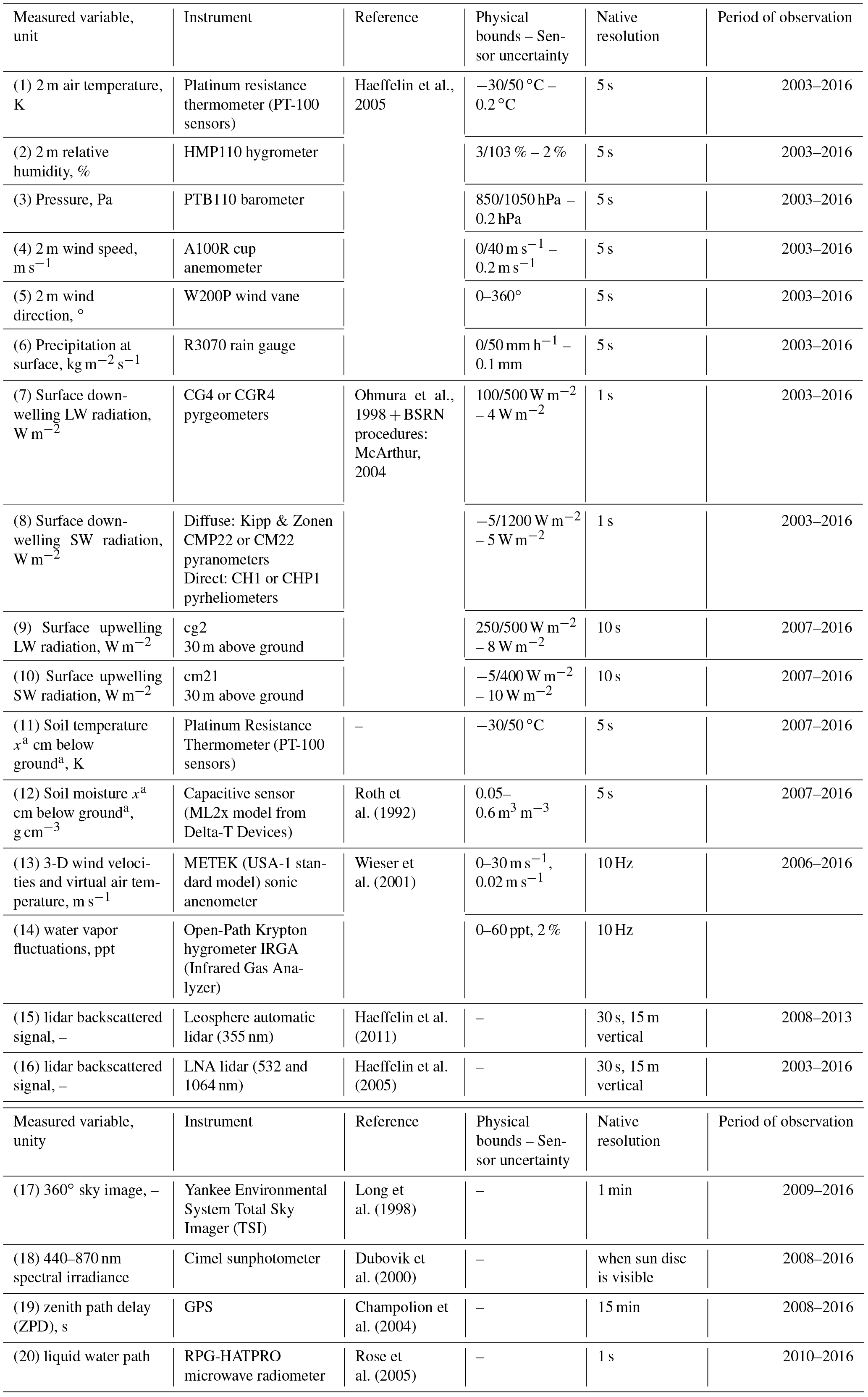
a x is 5, 10, 20, 30, 50 cm.
Table 2Variables included in SIRTA-ReOBS. First block (category A) is for classical meteorological measurements, second block (category B) is for more advanced measurements, third block (category C) is for parameters retrieved from observations and fourth block (category D) is for vertical lidar measurements.
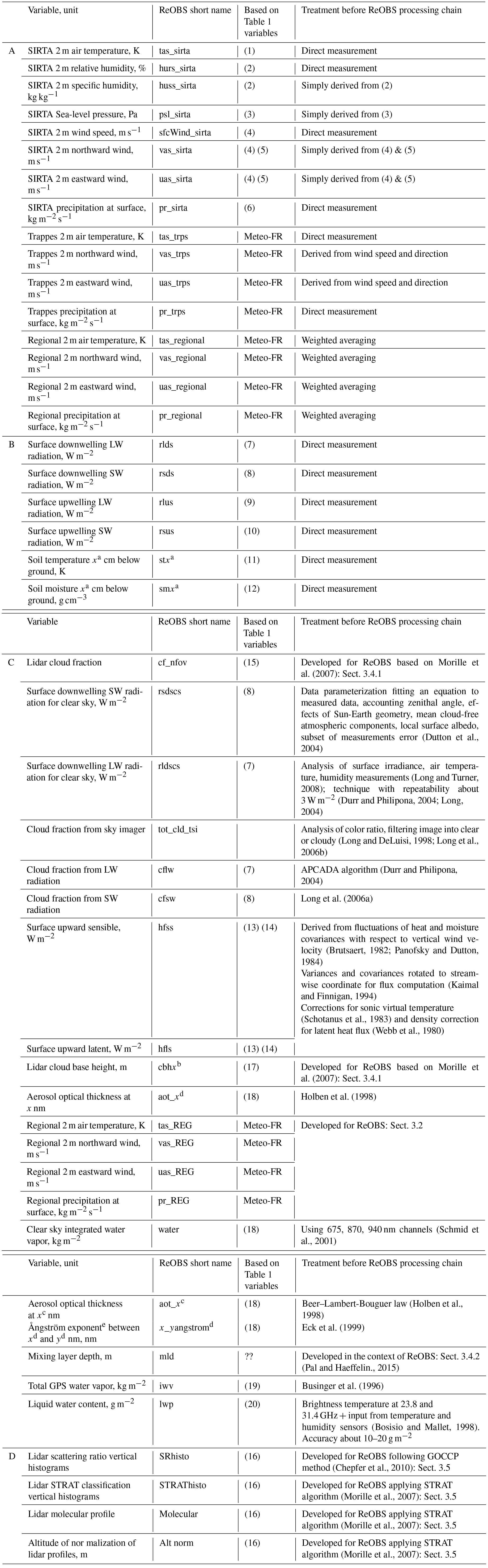
a x is 5, 10, 20, 30, 50 cm;
b x is first layer (1), second layer (2),
third layer (3);
c x is 1020, 870, 675, 500, 440, 380, 340 nm;
d x and y are the interval between c values.
e negative slope (or first derivative) of aerosol optical depth
with wavelength in logarithmic scale is the Angstrom parameter (Eck et al., 1999, see Fig. 4r for significance value).
Variables entering the ReOBS dataset are quality-controlled at their native time resolution. The quality control test consists of verifying that the variable lies within physical bounds (Table 1). Calculations of hourly mean and standard deviation only use native resolution data that have passed quality control. A simple informative quality flag is associated with each hourly value of a variable:
-
0: quality control is OK.
-
1: there are valid data but for less than 50 % of the period (that is, for less than 30 min).
-
2: flag 2 is only used for internal control and is never used as an informative output in the ReOBS file.
-
3: data is unavailable for the entire hour (no measurements or less than 50 % of the measurements in the hour passes the quality control). In this case, the hourly value is set by convention to −999.96.
Besides the systematic quality tests described above, some additional complementary quality controls have been applied to specific variables, as described in the following subsections (Sects. 3.2 to 3.5).
3.2 Specific computations for standard meteorological variables
Classical meteorological variables collected at three different locations are included in the ReOBS dataset: (1) the first group of variables is collected at the SIRTA supersite and has the advantage of being representative of the very local meteorology since the beginning of the supersite activities, (2) the second group of variables aims at characterizing the surrounding meteorology around the SIRTA site and (3) the third group of variables is from the standardized Météo-France station, collected at Trappes, 15 km away from the SIRTA supersite. These three different datasets are identified with the suffixes -sirta, -regional and -trps, respectively, in the following.
3.2.1 Description of surrounding meteorology around the SIRTA site
Figure 3b–d illustrate the air temperature, wind speed, and cumulated precipitations probability density functions (PDFs) in relative occurrence at three Météo-France stations within a 50 × 50 km domain around the SIRTA supersite: in Trappes (48.8∘ N, 2.0∘ W), in Paris-Montsouris (48.8∘ N, 2.3∘ W) and in Orly (48.7∘ N 2.4∘ W); these plots highlight the eventual differences from one site to another.
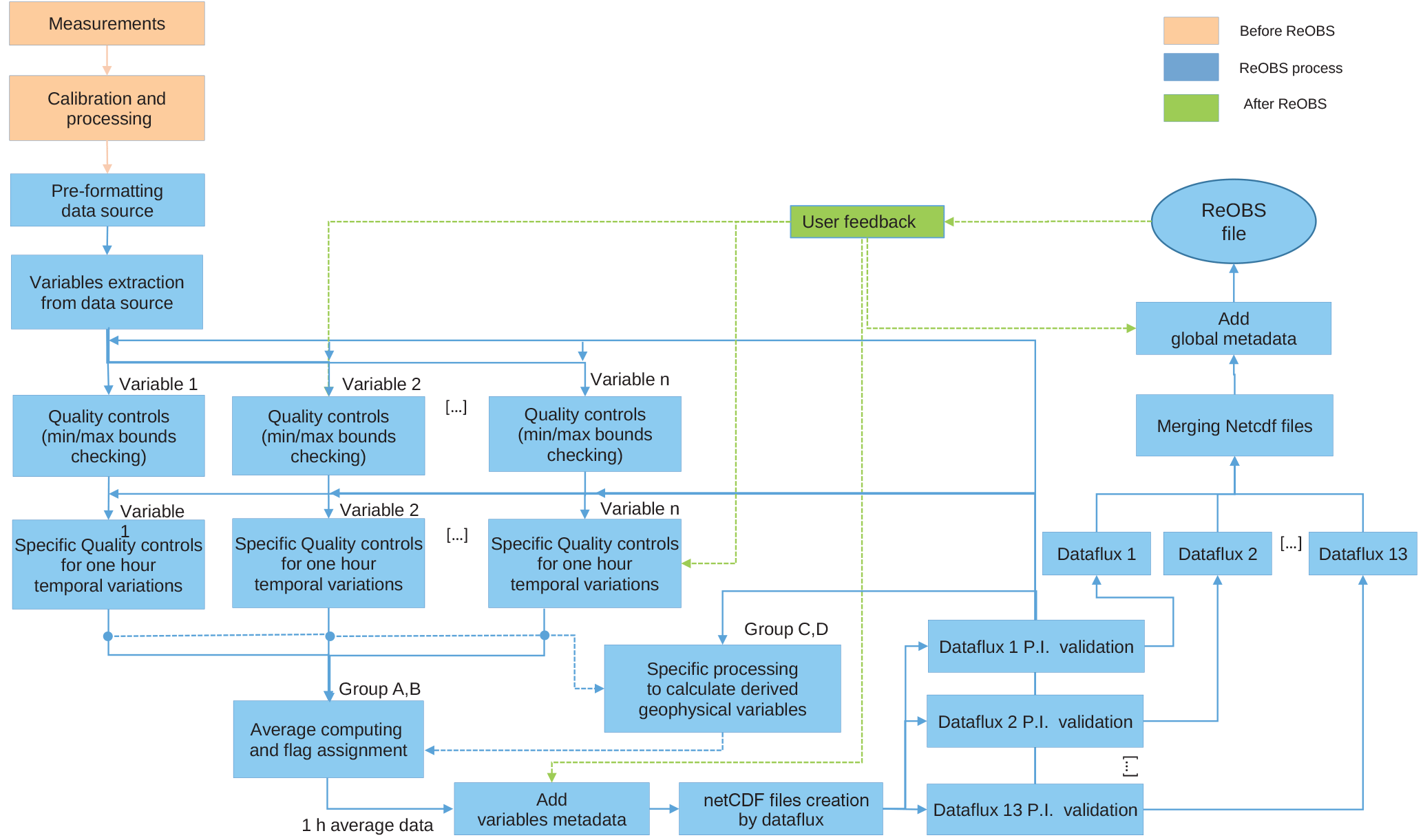
Figure 2Schematic of the ReOBS general processing chain. Orange, blue, and green boxes and arrows are for steps before, during, and after, respectively, the ReOBS processing chain.
The PDF of the 2 m air temperature (noted tas in SIRTA-ReOBS) shows an offset of about 2 ∘C for the Paris-Montsouris site compared to the Orly, Trappes and SIRTA sites, which is due to the urban heat. Maximum values for the mean wind speed value (noted sfcWind in SIRTA-ReOBS) are measured at the Orly site and the mean wind speed is around 3 m s−1 at SIRTA. Note that measurements at the SIRTA site are performed over a roof: wind speed is thus measured at 10 m above the roof, corresponding to 25 m above ground level, whereas it is measured at 10 m above ground level for the other stations. Even if a ground level standard (Météo-France-like) meteorological station is also present at SIRTA, the rooftop measurements were preferred for the ReOBS file because they started earlier (in 2003) than the standard meteorological station (in 2006). The four stations are characterized with a cumulated annual precipitation ranging between 600 and 700 mm yr−1.
The data collected at the three stations around the SIRTA supersite are used to characterize the surrounding 2 m meteorology. A weight is assigned to each of the three stations based on the following method: the 50 km× 50 km domain is divided into 90 × 103 grid boxes (300 × 300), the distance between each box and each site is calculated and then each box is linked to its nearest site. Then the percentage number of boxes linked to each site gives the weight of the site within the domain. The weight of the Trappes station is then 44.4 %, the weight of the Orly station is 34.5 % and the weight of the Paris-Montsouris station is 21.1 % (Fig. 3a). The regional-scale meteorology variables v (−REG) included in ReOBS are then obtained from
where is the set of values taken by a variable v (2 m temperature, humidity, wind, etc.) at each of the four stations, and is the station weight.
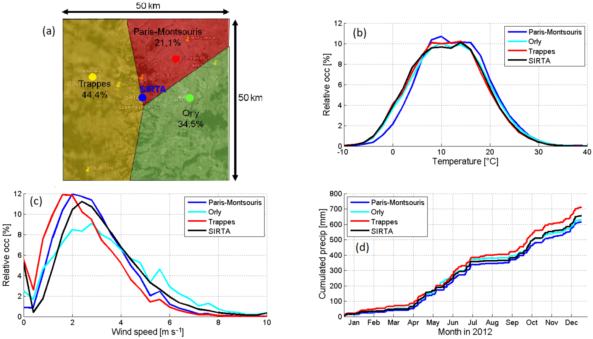
Figure 3(a) Location of the SIRTA supersite and the three neighboring Météo France stations with their associated weight as defined in the text. Relative occurrence of hourly mean air temperature (b) and wind speed (c) at SIRTA and at the neighboring Météo France stations between 2005 and 2014, and cumulated precipitation at SIRTA and at the neighboring Météo France stations in 2012 (d).
3.2.2 Quality control of the standard meteorological variables
The quality control for meteorological variables listed in Table 2 consists of two additional tests compared to what was indicated in Sect. 3.1. The goal of the quality control is to reject unphysical values and to reject values with unrealistic temporal variability (Tables 1 and 3), e.g., non-physical jump in the data record, non-physical persistence in time of the measured values.
Non-physical jumps in the data are detected at native high temporal resolution (5 s). If the difference between two successive measurements is more than a specified limit given in Table 3 (these tests are about to be refined in a new study that will give a new version of the SIRTA-ReOBS file) the current measurement is rejected but it is used for checking the temporal consistency with the next measurement. Two examples of measurements that did not pass the quality control tests are shown in Fig. 4a and b for pressure and soil temperature jumps, respectively. In the first example, an unphysical change of 2 hPa within 1 min is observed in pressure (larger than 5 hPa during 5 min, see Table 3). In the second example, several temperature spikes (0.6 ∘C within 1 min for ground at −5 cm) are detected and we reject the data when the increase reaches +3 ∘C and the decrease −4 ∘C within 15 min (i.e., +0.2 and −0.27 ∘C for 1 min resolution).
The unphysical persistence in time of the measured values are detected by verifying that the variability within 1 hour is physical, following values in Table 3. If the 1-minute values do not vary by more than a specified lower limit (given in Table 3) within 1 hour, the current value fails the check. Figure 4d shows an example of an unphysical wind speed measured by a cup anemometer. The value is 0 m s−1 after 18:00 UT because of frost deposition on the sensor (shown by low temperature and high relative humidity in Fig. 4c). The persistence test is completed by a calculation of the standard deviation of temperature, pressure, humidity and wind speed for the last 1-hour period. In combination with the persistence test, the evaluation of the standard deviation is a very good tool for the detection of a blocked sensor, as well as a 1 h sensor drift.
3.3 Specific computation for advanced meteorological variables
The data quality of in-ground temperature and permeability of the soil is checked using the tests above (Table 1 and 3).
The quality of the downwelling shortwave (SW) and longwave (LW) fluxes is tested following the recommendation of the Baseline Surface Radiation Network (BSRN; test version 2.0; Roesch et al., 2011). Additional semi-automatic controls were developed and applied to SW irradiances in order to reject data collected when the sun tracker failed (used for the direct and diffuse SW radiation measurements) and to remove values that are inconsistent between measured global SW fluxes and global SW fluxes calculated from direct and diffuse measured ones. Individual 1 min native data not passing the test are automatically removed before performing the 1 h averages. For SW fluxes, the global as well as the direct and diffuse irradiance components are included in the ReOBS dataset. A best estimate of the global SW is calculated as a combination of the global irradiance measurement and the sum of the diffuse and horizontal direct irradiance measurements. The sum is taken as default and the blanks in observations are filled with the global irradiance measurement.
The sensible and latent heat flux data are subjected to spike detection and rejection algorithms. Sensible and latent heat fluxes are based on sonic measurements and a gas analyzer. The lag between the sonic measurements and the gas analyzer is set to the lag of maximum correlation over the averaging interval between the sonic anemometer temperature and the absolute humidity measured by the gas analyzer. At hourly intervals, sensible and latent heat fluxes are derived from eddy-covariance techniques, as well as turbulence statistics. Raw data and calculated statistics are subjected to strict data limits to reject unphysical values (13 and 14 in Table 1). For the latent heat flux, the open-path infrared gas analyzer (IRGA) used between 2005 and 2012 could be damaged by precipitations and was therefore manually switched on and off. The temporal sampling was thus relatively low and we decided to exchange the IRGA with an open-path LI-COR LI-7500 in 2012. With the open-path InfraRed Gas Analyser the molar density fluctuations are accounted for in the processing by following the classic formulation of Webb et al. (1980). Moreover, an automatic method has been applied to correct wind statistics for any misalignment of the sonic anemometer with respect to the local wind streamlines of the sonic anemometer with respect to the local wind streamlines according to Wilczak et al. (2001).
3.4 Retrievals based on remote-sensing measurements developed for ReOBS
3.4.1 Computations for the cloud fraction and cloud base height from lidar
The ReOBS dataset contains cloud base height and time series of the cloud fraction (CF), deduced from the SIRTA 355 nm lidar and processed with the STRAT algorithm (STRucture of the ATmosphere; Morille et al., 2007). The cloud fraction (noted cf_nfov, where “nfov” stands for “narrow field of view”) is defined as the number of profiles containing clouds divided by the total number of profiles collected in 1 hour. The cloud base height of the first layer (noted CBH1) corresponds to the altitude of the first cloud layer from the ground as detected by the STRAT algorithm. An hourly cloud base height is reported in ReOBS only if at least 33 % of the profiles collected during this hour are cloudy and only if less than 40 % of the profiles collected during this hour are noisy (i.e., at least 60 % of profiles are valid). Sensitivity tests based on several case studies have shown that taking less than this 33 % or more than this 40 % threshold leads to cloud base height values non-representative of what happens in the current hour. CBH2 and CBH3 are the altitudes of the base of a second and a third cloud layer, respectively, detected above CBH1 and separated from the first cloud (the one with CBH1) with clear sky.
3.4.2 The mixing layer depth product
The mixing layer depth (MLD, noted mld in SIRTA-ReOBS) is part of the SIRTA-ReOBS database. It is retrieved from routine lidar measurements (ALS 450 from the Leosphere company) following the method described in Pal et al. (2013) and Haeffelin et al. (2012).
In this method, the intensity of the lidar-derived aerosol backscatter signal at different altitudes is used to determine the hourly-averaged vertical profiles of variance. Next, the location of maximum turbulent mixing within the mixing layer is determined and corresponds to the mean MLD. Micrometeorological measurements of the Monin–Obukhov length scale are used (effect of buoyancy on turbulent flow; Monin and Obukhov, 1954) to better determine the MLD, especially for the early morning transition and evening transition periods. For these two specific periods, a first-order approximation of the boundary layer growth rates is obtained and the variance-based results guides the attribution by searching the minimum altitude of the gradient closest to the mean MLD. Two transition periods of a day are used to distinguish the turbulent regimes during the well-mixed convective ABL (atmospheric boundary layer) and nocturnal or stable MLD.
Table 3Range of temporal variabilities considered when performing the quality control for the variables listed in table. Upper arrows mean an increase during the time window indicated, and lower arrows mean a decrease during the time window indicated.
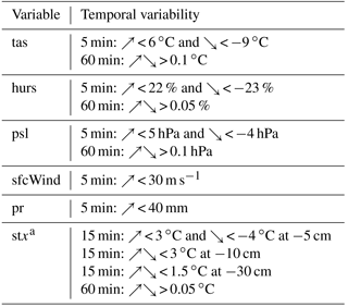
a x is 5, 10, 20, 30, 50 cm.
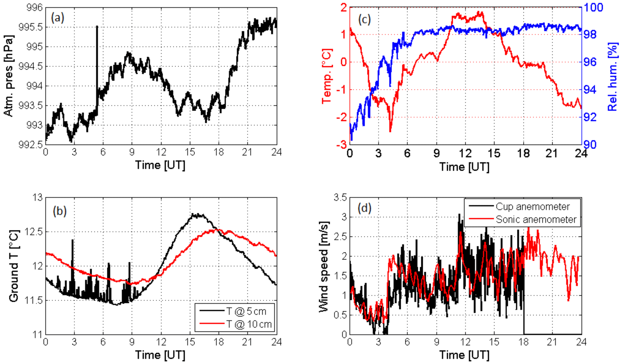
Figure 4(a) Example of an unphysical jump in instantaneous values of pressure and (b) temperature in ground at 5 cm (black) and at 10 cm (red). (d) Example of unphysical persistence of high wind speed measurements using a cup anemometer due to frost in (c) (negative temperature in red and high humidity values in blue).
3.5 Computations for the lidar profiles
The SIRTA ReOBS dataset contains information on the detailed vertical description of the atmosphere since 2002 from the LNA instrument. A drawback of this instrument is that it requires human intervention and does not operate when it rains, which introduces gaps in the data record.
Two different hourly variables are included in the ReOBS dataset:
-
One variable called STRAThisto, which contains the number of occurrences of clear sky, aerosols, clouds, invalid data and fully attenuated laser within 1 hour for each vertical level. The vertical resolution is 15 m up to 15 km and the layer type classification is based on the STRAT algorithm.
-
One variable called SRhisto is a 2-D height-intensity number of occurrences accumulated during 1 hour, as defined in Chepfer et al. (2010). We use the lidar scattering ratio SR = ATB ∕ ATBmol, where ATB is the total attenuated backscatter lidar signal and ATBmol is the signal in clear-sky conditions. The vertical resolution is 15 m and the intensity axis contains 18 bins; −999 / −777 / −666 / 0 / 0.01 / 1.2 / 3 / 5 / 7 / 10 / 15 / 20 / 25 / 30 / 40 / 50 / 60 / 80. The value “−999“ indicates non-normalized noisy profiles, the value “−777” is for profiles that cannot be normalized due to the presence of a very low cloud, and the value “−666” is for invalid data. ATB profiles are normalized to a daily molecular profile based on radiosounding measurements launched every day 10 km away from the SIRTA supersite (at the Météo-France station in Trappes). The altitude of normalization of ATB (which must be clear sky) is determined for each profile using the STRAT algorithm.
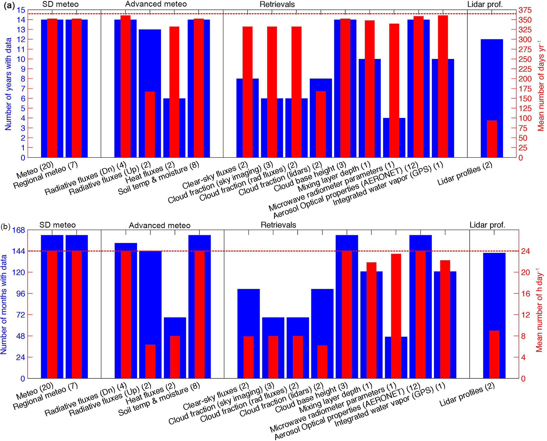
Figure 5Temporal coverage of groups of variables in the SIRTA-ReOBS dataset. In panel (a), blue bars indicate the total numbers of years with data and red bars indicate the mean numbers of days with measurements in a year. In panel (b), blue bars indicate the numbers of months with data and red bars indicate the mean numbers of hours with measurement in a day. The numbers in brackets are the number of variables in each sub-group. Variables are separated in four categories: classical meteorological measurements (group A, left), more advanced measurements (group B, center-left), variables retrieved from measurements (group C, center-right) and lidar profiles (group D, right). Dn means downward, Up means upward.
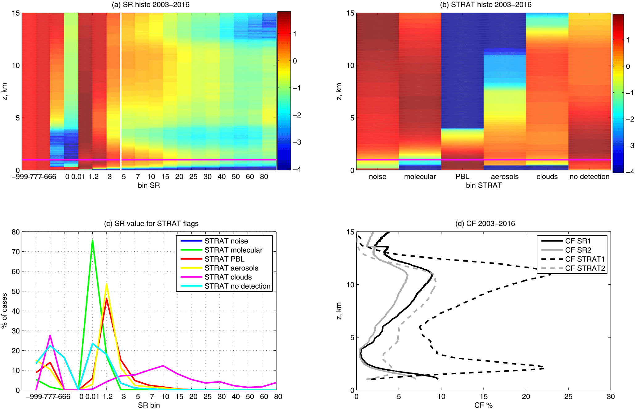
Figure 6(a) Lidar scattering ratio (SR) histogram obtained by cumulating all SIRTA observation data from 2003 to 2016. The color bar is the logarithm of the percentage of occurrence (the sum of one line is equal to log(100 %)); the pink horizontal line corresponds to the altitude of recovery of the lidar (z= 1 km; below this altitude, lidar data is more complicated to use); the white vertical line corresponds to the threshold of cloud detection (SR = 5). (b) STRAT histogram obtained by cumulating all data from 2003 to 2016. The color bar is the logarithm of the percentage of occurrence. (c) Percentage of occurrence of SR values for the different STRAT flags (noise in blue – no cases actually –, molecular in green, PBL in red, aerosols in yellow, clouds in magenta and no detection in cyan), cumulating all altitudes above 1 km and only for hours containing a single STRAT flag. (d) Fraction of clouds (in %): CF SR1 (black solid line) is the occurrence of SR > 5 versus the occurrence of SR > 0, CF SR2 (gray solid line) is the occurrence of SR > 5 vs. the total occurrence of profiles, CF STRAT1 (black dashed line) is the occurrence of STRAT cloudy profiles versus the occurrence of STRAT molecular + PBL + aerosols + cloud profiles, CF STRAT2 (gray dashed line) is the occurrence of STRAT cloudy profiles vs. the total occurrence of profiles.
4.1 Description of the ReOBS database content
All data passing the quality control tests are included in the ReOBS final netCDF file. The variables included in the SIRTA-ReOBS are listed in Table 2 together with their nomenclature (Table 2, second column). There are 42 lines in Table 2, corresponding to 34 variables currently in the file. Figure 5 shows the temporal coverage of each variable. Some variables such as the classical meteorological variables or the downwelling radiative fluxes are very well sampled since 2002 when SIRTA activities started. In contrast, the record for lidar profiles, which started in 2002, contains many gaps. The sampling of the latent heat flux is much more intermittent than the sampling of the sensible heat flux due to instrumental issues (see Sect. 3.3).
There are two versions of the SIRTA-ReOBS file: a complete file, which includes all information available (1.2 Gb), and another one which contains all data except for the vertical information from the lidar (11.5 Mb): this last is significantly smaller and so it is easier to handle. Both data files are available on the following website: http://sirta.ipsl.fr/reobs.html (Downloads tab, no password required), which also includes quicklooks and a documentation.
The main advantages of ReOBS compared to classical supersite databases are (1) the vertical profile information coming from lidar measurements, which is user friendly thanks to the GOCCP (GCM Oriented CALIPSO Cloud Product) method (Chepfer et al., 2010), (2) the possibility to study the troposphere at different timescales (from daily to decadal timescales) and (3) the availability of a multi-variable synergetic view of the atmosphere. And of course a mix of these three aspects. These three main added values are detailed in the following subsections.
4.2 Vertical profile information
The lidar profiles included in SIRTA-ReOBS provide useful information on the vertical distribution of clouds and aerosols in the atmosphere. This information together with many other SIRTA-ReOBS variables have been used recently in various studies (Cheruy et al., 2012; Chiriaco et al., 2014; Bastin et al., 2016). We first show examples of the two main ReOBS variables build from lidar measurements (SRhisto and STRAThisto) and we then describe how these data are used to built cloud fraction profiles. Finally, we describe how to use these data to evaluate clouds simulated by models.
4.2.1 SRhisto and STRAThisto
Figure 6 shows SRhisto (Fig. 6a) and STRAThisto (Fig. 6b) for every hour containing measurements from 2003 to 2016. Periods without lidar measurements are not included in this figure and this happens frequently (see Fig. 5) because measurements are only performed when it is not raining and with human intervention (i.e., not during night and weekends). Using SRhisto, the repartition of clouds can be analyzed as a function of altitude and as a function of the intensity of the lidar signal (SR), which is a proxy of the particle optical thickness. Fully attenuated lidar signals are located in the bin 0 < SR < 1, clear sky are found in the bin SR = 1, uncertain are in the bin 1 < SR < 5 (it could be aerosols for instance), and SR > 5 is for clouds (white vertical line in Fig. 6a; bins defined in Sect. 3.5). The analysis of SRhisto shows that non-precipitating clouds observed at SIRTA (note: the LNA lidar instrument does not operate when it rains) are mostly thin, low clouds (under 4 km with SR < 15) or thin, high clouds (above 7 km with SR < 20), and there are also thicker clouds with SR > 80 or fully attenuated lidar signal. There are almost no mid-level clouds (between 4 and 7 km) and only few clouds with 20 < SR < 80. The analysis of STRAThisto indicates that for these non-precipitating cases, the amount of clouds that fully attenuates the lidar signal (i.e., “noise”) is approximately on the same order of magnitude as the amount of thinner clouds.
Lidar profiles that would be measured in clear-sky conditions (so called molecular profiles) are necessary to build SRhisto and STRAThisto as it is used in the SR estimation and in the STRAT lidar profile normalization. These molecular profiles are estimated based on temperature and pressure profiles measured twice a day by METEO-FRANCE radiosounding at Trappes (10 km from SIRTA). These molecular lidar profiles are included in SIRTA-ReOBS under the Molecular variable, as well as the altitude of normalization used for STRAT under the Alt norm variable.
4.2.2 Cloud fraction profiles
Cloud fraction profiles are derived from the SRhisto or from the STRAThisto variables at a temporal scale ranging from 1 hour up to several years. At a given altitude level, the cloud fraction is the ratio between the occurrence of cloudy cases and the occurrence of all cases excluding the noisy ones. In STRAThisto the occurrence of cloudy layers is given in flag “clouds”. In SRhisto, a layer is declared cloudy in a lidar profile when SR > 5 and SR > 1+ε/ATBmol with ε= 1.3 × 10⁻⁶ SI (ATBmol is included in SIRTA-ReOBS). As expected, the cloud fraction profiles obtained from SRhisto or from STRAThisto (Fig. 6d) are different due to the differences in the definition of the cloud detection in the two algorithms. In particular, SRhisto features less low-level clouds (z < 4 km) than STRAThisto. The magenta curve in Fig. 6c is the SR distribution for cloudy cases during a given hour for the STRAT algorithm. This distribution shows that about 28 % of these cases correspond to cases where SR cannot be estimated because of the presence of a very low cloud (−777 in Fig. 6c) preventing the normalization of the profile (no detection of molecular signal under the cloud). This could explain the differences in low cloud fractions between STRAThisto and SRhisto in Fig. 6d. The part of the magenta curve with values of SR between 0.01 and 5 corresponds to cloudy cases for the STRAT algorithm but not based on the SR threshold method. This could explain the bias between CF SR and CF STRAT that occurs at almost all vertical levels. Red and yellow curves in Fig. 6c also highlight the fact that most of the cases that are defined as PBL or aerosols for the STRAT algorithm are actually not cloudy when based on the SR threshold method (the parts of these curves above SR = 5 represent less than 5 %). The differences between STRAT- and SR-based algorithms illustrate the important sensitivity of the cloud fraction profile to the cloud definition. This sensitivity needs to be taken into account when comparing the measurements to simulations from GCMs or RCMs in order to reproduce the algorithm hypotheses in the simulations; it is usually done using a lidar simulator described below.
4.2.3 Lidar simulator
For comparing the SIRTA-ReOBS SRhisto variable to GCM or RCM outputs, we have developed a ground-based lidar simulator, which is an adaptation of the CALIOP (Cloud-Aerosol Lidar with Orthogonal Polarization) lidar simulator (Chepfer et al., 2008), taking into account the specification due to the ground-based position of the instrument. In particular, the vertical turnaround of the lidar equation following the very first version of lidar simulator described in Chiriaco et al. (2006). Model outputs are used as inputs for the lidar simulator to simulate what would be measured from the ground-based lidar if the atmosphere was the simulated one. First the lidar equation that gives the ATB as a function of altitude is used to simulate SR from model outputs. Then the same space and time resolutions as in observations and the SR thresholds are used for the simulated lidar profiles as in the actual data algorithm (SRhisto for SIRTA-ReOBS), making the lidar profiles directly comparable to the measured ones.
This ground-based version of the lidar simulator has been used for comparisons between the SIRTA-ReOBS lidar profiles and the WRF/MED-CORDEX (Weather Research and Forecast model; Coordinated Regional Climate Downscaling Experiment for Mediterranean area) simulation in Bastin et al. (2016).
This lidar simulator is currently implemented in the new COSP2 simulator package (version 2 of COSP – CFMIP; Cloud Feedback Model Intercomparison Project, Observation Simulator Package; currently developed for CMIP6 simulations), following these steps: (1) computation of the molecular optical thickness of each layer (i.e., the atmosphere clear of any particles), (2) computation of the particles optical thickness of each layer, (3) computation of the total optical thickness of each layer by adding the molecular and the particles optical thicknesses, (4) computation of the total backscatter lidar signal as it would have been measured by a ground-based lidar by integrating progressively these optical thicknesses from the lowest atmospheric layer to the top of the atmosphere and (5) computation of the SR profile by dividing the attenuated total backscatter lidar profile by the clear-sky profile.
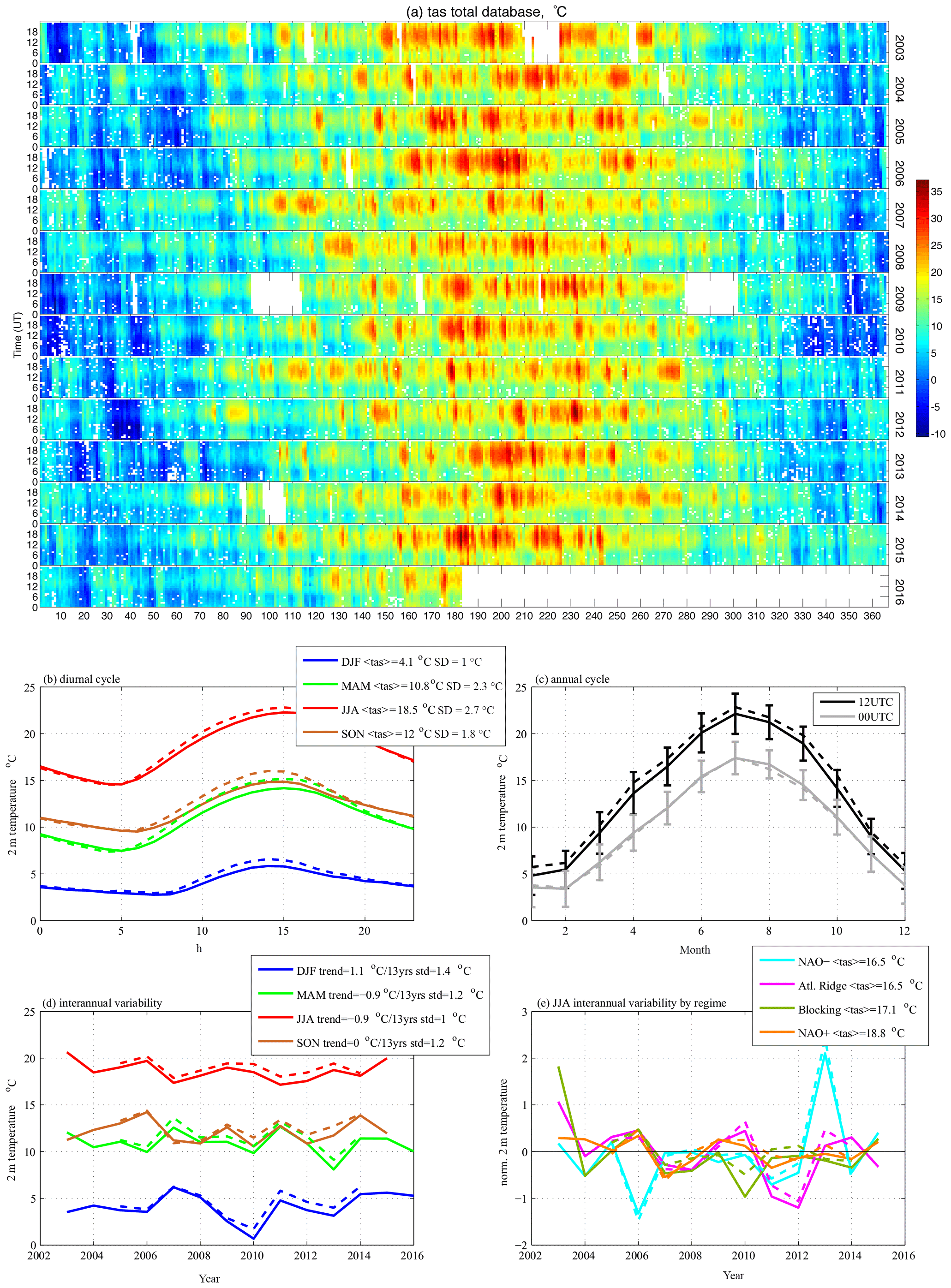
Figure 7Contribution of the multi-temporal scale for the 2 m temperature (in ∘C). (a) Hourly values, each row corresponds to a year with the day of the year in x axis, and the hour of the day in y axis. (b) Mean diurnal cycle averaged from 2003 to 2016 split into seasons (DJF in blue, MAM in green, JJA in red, SON in brown). The mean values and the standard deviation of the 2 m temperature in each season are indicated. (c) Mean annual cycle averaged monthly from 2003 to 2016 at 12:00 UTC (black line) and at 00:00 UTC (gray line) with interannual SD in error bars. (d) Interannual evolution from 2003 to 2016, averaged by season (same colors as b). The trends of the curve (i.e., the slope of the curve linear regression multiplied by the number of years – 13) and its standard deviation are indicated. (e) Same curve as in (d) for JJA only, split per weather regimes (NAO− in cyan, Atlantic Ridge in magenta, blocking in green, NAO+ in orange) and plotted in anomaly (i.e., the mean value of all years is subtracted), where “norm. T2” is calculated following the Eq. (2). In all panels, solid lines are for the SIRTA local 2 m temperature, and dashed lines are for the regional 2 m temperature (around the SIRTA supersite).
4.3 From the daily timescale to the decadal timescale
The temporal variability in the variables included in SIRTA-ReOBS is synthesized in a single figure, as shown in Fig. 7a for the 2 m temperature. Each row represents a year and in each row, the x axis indicates the day of the year and the y axis indicates the hour of the day. This figure allows for the visualization of the presence of gaps in the record and the different temporal scales of variability: diurnal, seasonal and interannual. A first visual inspection leads to the identification of significant anomalies in terms of amplitude and in terms of persistence. Figure 7b shows the mean temperature diurnal cycle split by seasons. Solid lines indicate the local SIRTA temperature (−SIR) and dashed lines indicate the surrounding temperature (−REG, Sect. 3.2.). Since air temperature is at first order controlled by radiation, the coldest season is winter (mean value 4.1 ∘C) followed by spring (10.8 ∘C), fall (12 ∘C), and summer (18.5 ∘C), as expected. The amplitude of the diurnal cycle is greater in summer (standard deviation of 2.7 ∘C), than spring (SD =2.3 ∘C), fall (SD =1.7 ∘C) and winter (SD =1 ∘C). The specificity of SIRTA seems to lead to an attenuation of this diurnal cycle, as it is less pronounced than in the surrounding areas (note that temperatures during daytime are lower at SIRTA than in the surroundings, whereas they are equivalent during the night), likely due to urban, vegetation or soil moisture effects. Figure 7c shows the mean annual cycle of the 2 m temperature at 12:00 UTC (noon; black lines) and at 00:00 UTC (midnight; gray lines). As for the diurnal cycle, differences between local SIRTA measurements (solid lines) and regional 2 m temperature (dashed lines) are more pronounced at noon than at midnight. Figure 7d shows the interannual variability in the 2 m temperature split into seasons. There is no significant trend in the four seasons (the linear regression of each of the four curves multiplied by the number of years is weaker than 1σ, where σ is the SD, of the curve). Nevertheless, significant temperature anomalies are detected such as the cold winter 2010, the cold spring 2013, the warm fall 2006, the warm winter 2007 or the hot summer 2003. Summer mean values are split into weather regimes following the classification of Yiou et al. (2008) from the A2C2 (Atmospheric flow Analogues for Climate Change) project. In summer at SIRTA, the daily temperature is maximal when the weather regime is NAO+ (North Atlantic Oscillation+), it is weaker when the weather regime is blocking or NAO− and it is minimal when the weather regime is “Atlantic Ridge”, as expected based on literature (numbers in the box in Fig. 7e). The anomaly (i.e., the mean value of all years is subtracted from each year value) of V(y,ri) for June–July–August in a given year y and a given regime ri (where ri is one of the four weather regimes mentioned above) plotted in Fig. 7e is calculated as follows:
where <tas(y,ri)> is the mean value of the 2 m air temperature in year y and for days in regime ri, and SD(tas(y,ri)) is its standard deviation. Hence V(y,ri) is a mean temperature normalized by its variability and is unitless. Using this estimation, strong anomalies (i.e., anomalies that have a strong standard deviation) due to only a few numbers of days are minimized. This representation shows that summers that are not particularly warm or cold could actually contain significant anomalies. During summer 2013 for instance, NAO− days have been significantly warmer than NAO− days of the other summers, meaning that during these particular days, the temperature anomaly was due to processes and not only due to the large-scale circulation condition.
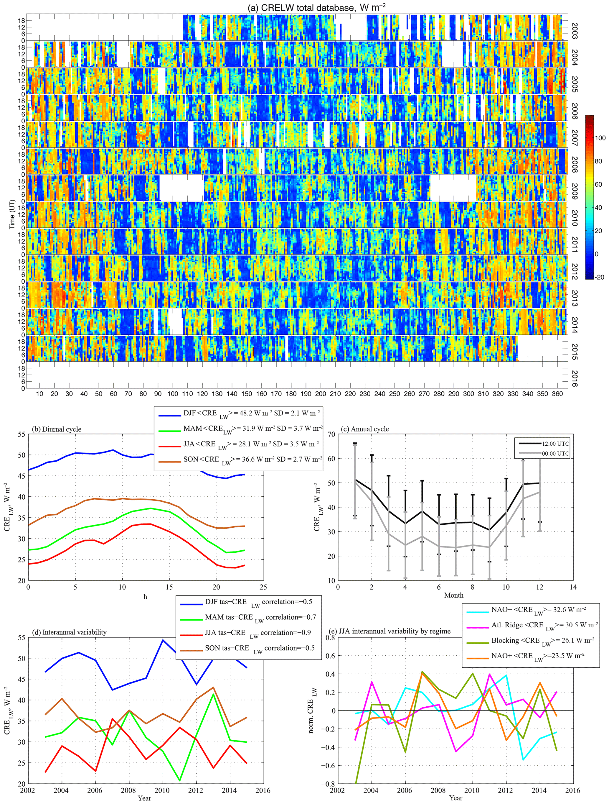
Figure 8Same as Fig. 7 but for the longwave cloud radiative effect (in W m−2). In panel (d), the correlation between values in Fig. 7d (tas) and values in Fig. 8d (CRELW) are indicated.
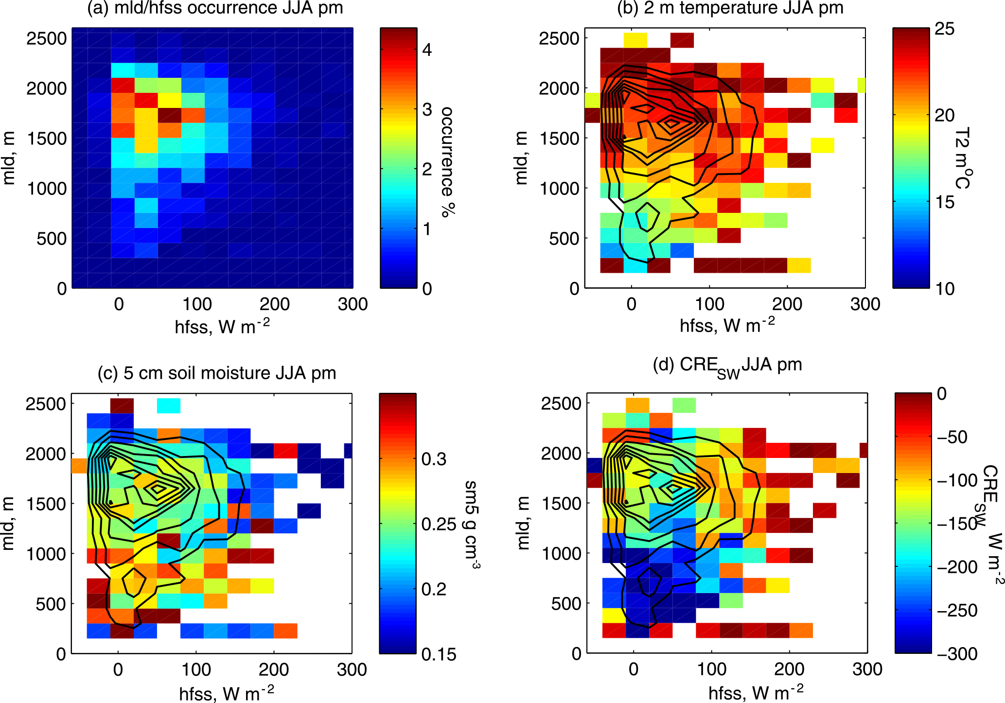
Figure 9(a) Occurrence distribution (in percent) of the mixing layer depth (y axis) and the sensible heat flux (x axis) variables in summer (JJA) for the afternoon (02:00 to 06:00 LST). Averaged 2 m temperature (b), averaged soil moisture at 5 cm depth (c), and averaged shortwave cloud radiative effect (d). Data are cumulated before the averaging. Black contours in (b), (c) and (d) are isolines of (a): the outermost isoline indicates 0.5 % of occurrence and each curve is then incremented of 0.5 %, and the innermost curve corresponds to 4 %.
Figure 8 is the same as Fig. 7 but illustrates the cloud radiative effect (CRE) in the longwave by the following equation:
where rlds and rldscs are the downward all-sky and clear-sky LW flux as defined in Table 2. Figure 8a highlights the fact that the database only has few gaps for these variables. It also shows that the diurnal cycle does not seem to be very intense (about 5 W m−2 amplitude in DJF: December–January–February and SON: September–October–November; and about 10 W m−2 in JJA: June–July–August and MAM: March–April–May), whereas the annual cycle is significant (about 25 W m−2 difference between summer and winter, in particular during the night). Figure 8a–d show that clouds have a stronger radiative effect in the longwave during winter than during the other seasons regardless of the hour of the day, for every year. It could simply be due to the amount of clouds that occur more often during winter, or due to cloud radiative properties that are different between the seasons. This variable does not have a significant trend from 2003 to 2015 for all season (i.e., the trend is smaller than the standard deviation). Nevertheless, the mean seasonal values are significantly anti-correlated to the temperature values in spring (−0.7) and in summer (−0.9). At first order, the CRELW is driven by the amount of clouds, and the more clouds the cooler the temperature. This anti-correlation is less pronounced in winter and fall (−0.5). This is explained by the fact that (1) the temperature variability must be driven by the air mass circulation more than by clouds and that (2) in winter there is less solar radiation even if there are no clouds so the difference between a clear-sky day and a cloudy day is not as pronounced as in summer. Particular anomalies of CRELW can be related to the temperature ones: for instance winter 2007 was particularly mild (Fig. 7d) and was associated with weak longwave cloud radiative effect (Fig. 8d) that could be due to a deficit of clouds. On the contrary, winter 2010 was colder than other winters in the period of study and is associated with strong CRELW. This correlation is also observed in summer (e.g., summers 2007 and 2011 are cold and have strong CRELW). The distinction of CRELW for each of the four weather regimes in summer (Fig. 8e) shows the part of the CRELW anomaly that is not due to the large-scale dynamical conditions, which is the first order driver. The 2013 positive temperature anomaly for NAO− cases is associated with an important deficit of CRELW in this weather regime.
4.4 Multi-variables synergetic view of the atmosphere
One of the main advantages of ReOBS is that all variables are synthesized in a single file at the same temporal resolution, facilitating studies with multi-variable synergy, particularly useful for the understanding of atmospheric processes. This synergy aspect has been exploited in previous studies using the SIRTA-ReOBS data; for instance to study the diurnal cycle, the annual cycle and the interannual variability but for multiple variables, (Cheruy et al., 2012 and Bastin et al., 2016), to study the different components and scales of the mixing layer depth variability (Pal and Haeffelin, 2015), and to perform in addition a dynamical analysis (Dione et al., 2016 and Chiriaco et al., 2014).
Figure 9 illustrates a possible synergy of multi-variables. The distribution of three variables affecting boundary layer processes in summer (JJA) is plotted (colors) as a function of mixing layer depth (y axis) and sensible heat flux (x axis) in the afternoon (between 02:00 and 06:00 LST, local solar time). The occurrence distribution of mixing layer depth versus sensible heat flux is reported in Fig. 9a and then as black contours in each other subplot: each isoline represents an increment of 0.5 %; pixels outside the most external isoline represent less than 0.5 % of the cases (per pixel). The 2 m temperature distribution is shown in Fig. 9b soil moisture at 5 cm depth on the middle one, and the cloud radiative effect on shortwave fluxes (CRESW) on the bottom one.
Figure 9a shows that shallow boundary layers (altitude of 500–1000 m) in summertime afternoon are mostly associated with low values of sensible heat flux (0–50 W m−2). They are associated with strong values of shortwave cloud radiative forcing (< −200 W m−2) due to the presence of clouds, high soil moisture (> 0.25 g m−2) and low air temperatures (< 17 ∘C). Deeper boundary layers (altitude of 1500–2000 m) are associated with a wide range of sensible heat fluxes (50–150 W m−2) and generally higher air temperatures (> 22 ∘C). For these deeper boundary layer cases, soil moisture and shortwave cloud radiative forcing are found to vary significantly.
The role of clouds in the link between mld and hfss can be easily identified in Fig. 9. In absence of clouds (CRESW close to zero), mld and hfss both have a high amplitude, while they both have a weak amplitude in the presence of clouds with strong albedo effect (CRESW < −200 W m−2). The occurrence of clouds with strong albedo effect correlates well with low temperatures and high soil moisture values.
However, most occurrences (black contours) correspond to low hfss, relatively high mld and intermediate values of CRESW. Temperatures are generally quite high also, and sm5 also presents intermediate values. Very clear-sky and dry-soil conditions (CRESW > −50 W m−2 and sm5 < 0.2 g m−2) generally lead to strong sensible heat fluxes and high temperatures, which do not necessarily translate into higher mixing layer depths than under cloudier conditions.
In summary, low mld are induced by strong cloud albedo effect and thus by low temperature and weak sensible heat flux due to weak energy reaching the surface. On the contrary, at hourly timescale, a mld higher than 1500 m is associated with a temperature higher than 20 ∘C and a wide range of CRESW (although greater than −200 W m−2). But this mld can be associated with a weak sensible heat flux. One reason for this is that the dominant timescale of variability for the boundary layer depth is the daily timescale, the maximum value being reached generally near 16:00 UTC in summer above SIRTA (Pal and Haeffelin, 2015), while the timescale of variability of the boundary layer forcers is hourly or less (radiative and heat fluxes). The temporal variability around the mld maximal value is often weak during this time lapse because it reacts with a delay. The energy dissipation rate in the boundary layer is slow and then the boundary layer stays deep even after the solar energy starts to decrease. So there is a delay between the decrease in mld and the decrease in the sensible heat flux. When considering the hourly timescale, many cases have high mld and low hfss. Investigating this issue in detail using the ReOBS database is beyond the scope of this paper.
The ReOBS processing chain has been applied to SIRTA ground-based measurements and leads to the production of a single netCDF file containing about 60 substantial geophysical variables hourly averaged over a period of up to a decade. The netCDF file is available at http://sirta.ipsl.fr/reobs.html under https://doi.org/10.14768/4F63BAD4-E6AF-4101-AD5A-61D4A34620DE.
We have presented a set of methods available for the community to robustly process ground-based data at an hourly timescale over more than a decade. The ReOBS processing chain has been applied to SIRTA ground-based measurements and leads to the production of a single netCDF file containing about 60 substantial geophysical variables hourly averaged over up to a decade. The netCDF file is available at http://sirta.ipsl.fr/reobs.html under https://doi.org/10.14768/4F63BAD4-E6AF-4101-AD5A-61D4A34620DE.
The main implication of this work is that complex observations are made available for the scientific community and allow for multiannual and multi-variable studies combining atmospheric dynamics and thermodynamics, radiation, clouds and aerosols. For example, the variability in 2 m temperature and LW cloud radiative effect can be jointly studied on the diurnal up to the interannual timescales. The multi-variable synergy is also illustrated with a focus on the boundary layer processes. As mentioned before, SIRTA-ReOBS has been already used in previous published studies: Cheruy et al. (2012) and Bastin et al. (2016) used SIRTA-ReOBS to evaluate simulations from GCMs and from RCMs, respectively. In these studies, using SIRTA-ReOBS has led to identifying the processes responsible of the model biases. Still in term of processes, Pal and Haeffelin (2015) used SIRTA-ReOBS to study the different components and scales of the mixing layer depth variability. Dione et al. (2016) and Chiriaco et al. (2014) have benefited from the SIRTA-ReOBS to study specific season anomalies. Datasets from ReOBS method are also useful tools for teaching and outreach activities such as the European KIC-Climate summer Journeys of the LABEX L-IPSL (Laboratory of Excellence Institut Pierre Simon Laplace) or the CLE-workshop (CLimate and Environment).
The ReOBS processing chain is now complete but the produced files such as SIRTA-ReOBS are continuously being improved, e.g., by adding new periods of data, by treating new variables and by improving the quality control. The SIRTA-ReOBS file presented in this paper is at a precise time. Future development for SIRTA-ReOBS include (1) improving the quality control of classical meteorological variables based on a comparative study of different methods, (2) adding vertical profiles from radiosounding launched twice a day 10 km away from the SIRTA supersite since the 90s and (3) adding new variables such as cloud radar data, gases and wind profiles from radar and lidar.
The ReOBS approach described in this paper will be applied to other supersites. Applying this approach to data from supersites of the ACTRIS-FR (Aerosol Cloud and Trace Gases Researche Infrastructure – France) infrastructure, in particular to the P2OA site located in the south of France is currently being tested. Applying ReOBS to ACTRIS-EU supersites is also under discussion. Another ongoing project is to integrate the ReOBS dataset to the OBS4MIP (Observations for Model Intercomparisons Project) database, which contains the data collected from observations developed specially for comparisons to CMIP simulations. This requires only few adaptations to fit the OBS4MIP standards.
The authors declare that they have no conflict of interest.
The authors would like to thank the following for financial support: Ecole Polytechnique, IPSL, FX-Conseil and the European project EUCLIPSE (European Union Cloud Intercomparison, Process Study and Evaluation project) for ReOBS since the beginning of this project. This study also benefited from the support of the Labex L-IPSL, which is funded by the Agence Nationale pour la Recherche (grant no. ANR-10-LABX-0018).
The authors would like to thank IPSL mesocenter and ESPRI teams from IPSL for providing computing and storage resources, and the SIRTA for providing measurements and data.
This work is also a contribution to the EECLAT project through LEFE-INSU and CNES supports, as well as to ACTRIS-FR, which is a national distributed research infrastructure and identified on the French road map for Research Infrastructures, published by the Ministry of Research. ACTRIS-FR is coordinated by the CONSORTIUM ACTRIS-FR and comprises a large number of French research organizations and institutions.
Marjolaine Chiriaco was partly supported by Centre National d'Etudes Spatiales (CNES) until 2016.
The authors would like to thank the A2C2 European project for providing the
weather regimes classification (ERC advanced grant no. 338965 – A2C2 ).
Edited by: David Carlson
Reviewed by: two anonymous referees
Ackerman, T. and Stokes, G.: The Atmospheric Radiation Measurement Program, Phys. Today, 56, 38–45, 2003.
Bastin, S., Chiriaco, M., and Drobinski, P.: Control of radiation and evaporation on temperature variability in a WRF/MED-CORDEX simulation: comparison with collocated long term ground based observations near Paris, Clim. Dynam., https://doi.org/10.1007/s00382-016-2974-1, 2016.
Bosisio, A. V. and Mallet, C.: Influence of cloud temperature on brightness temperature and consequences for water retrieval, Radio Sci., 33, 929–939, 1998.
Brutsaert, W.: Evaporation into the atmosphere: theory, history and applications., D. Reidel Publishing Co., Norwell, MA, USA, 299 pp., 1982.
Businger, S., Chiswell, S. R., Ulmer, W. C., and Johnson, R.: Balloons as a Lagrangian measurement platform for atmospheric research, J. Geophys. Res., 101, 4363–4371, https://doi.org/10.1029/95JD00559, 1996.
Chepfer, H., Bony, S., Winker, D., Chiriaco, M., Dufresne J.-L., and Sèze, G.: Use of CALIPSO lidar observations to evaluate the cloudiness simulated by a climate model, Geoph. Res. Lett., 35, L15704, 2008.
Chepfer, H., Bony, S., Winker, D., Cesana, G., Dufresne, J. L., Minnis, P., Stubenrauch, C. J., and Zeng, S.: The GCM Oriented Calipso Cloud Product (CALIPSO-GOCCP), J. Geophys. Res., 115, D00H16, https://doi.org/10.1029/2009JD012251, 2010.
Cheruy, F., Dupont, J. C., Campoy, A., Ducharne, A., Hourdin, F., Haeffelin, M., and Chiriaco, M.: Combined influence of atmospheric physics and soil hydrology on the realism of the LMDz model compared to SIRTA measurements, Clim. Dynam., 40, 2251–2269, https://doi.org/10.1007/s00382-012-1469-y, 2012.
Chiriaco M., Vautard, R., Chepfer, H., Haeffelin, M., Dudhia, J., Wanherdrick, Y., Morille Y., and Protat, A.: The Ability of MM5 to Simulate Ice Clouds: Systematic Comparison between Simulated and Measured Fluxes and Lidar/Radar Profiles at SIRTA Atmospheric Observatory, Mon. Weather Rev., 134, 897–918, 2006.
Chiriaco, M., Bastin, S., Yiou, P., Haeffelin, M., Dupont, J.-C., Klenov, L., and Stéfanon, M.: European heat-wave in July 2006: observations and modelling showing how local processes amplify conducive large-scale conditions, Geophys. Res. Lett., 41, 5644–5652, 2014.
Dione, C., Lohou, F., Chiriaco, M., Lothon, M., Bastin, S., Baray, J.-L., Yiou, P., and Colomb, A.: The influence of synoptic circulations and local processes on temperature anomalies over three French observatories, JAMC, 58, 141–158, https://doi.org/10.1175/JAMC-D-16-0113.1, 2017.
Dubovik, O. and King, M. D.: A flexible inversion algorithm for retrieval of aerosol optical properties from sun and sky radiance measurements, J. Geophys. Res., 105, 20673–20696, 2000.
Durr, B. and Philipona, R.: Automatic cloud amount detection by surface longwave downward radiation measurements, J. Geophys. Res., 109, D05201, https://doi.org/10.1029/2003JD004182, 2004.
Dutton, E. G., Farhadi, A., Stone, R. S., Long, C. N., and Nelson, D. W.: Long-term variations in the occurrence and effective solar transmission of clouds as determined from surface-based total irradiance observations, J. Geophys. Res., 109, D03204, https://doi.org/10.1029/2003JD003568, 2004.
Eck, T. F., Holben, B. N., Reid, J. S., Dubovik, O., Smirnov, A., O'Neill, N. T., Slutsker, I., and Kinne, S.: Wavelength dependence of the optical depth of biomass burning, urban and desert dust aerosols, J. Geophys. Res., 104, 31333–31350, 1999.
Haeffelin, M., Barthès, L., Bock, O., Boitel, C., Bony, S., Bouniol, D., Chepfer, H., Chiriaco, M., Cuesta, J., Delanoë, J., Drobinski, P., Dufresne, J.-L., Flamant, C., Grall, M., Hodzic, A., Hourdin, F., Lapouge, F., Lemaître, Y., Mathieu, A., Morille, Y., Naud, C., Noël, V., O'Hirok, W., Pelon, J., Pietras, C., Protat, A., Romand, B., Scialom, G., and Vautard, R.: SIRTA, a ground-based atmospheric observatory for cloud and aerosol research, Ann. Geophys., 23, 253–275, https://doi.org/10.5194/angeo-23-253-2005, 2005.
Haeffelin, M., Angelini, F., Morille, Y., Martucci, G., Frey, S., Gobbi, G. P., Lolli, S., O'Dowd, C. D., Sauvage, L., Xueref-Rémy, I., Wastine, B., and Feist, D. G.: Evaluation of Mixing-Height Retrievals from Automatic Profiling Lidars and Ceilometers in View of Future Integrated Networks in Europe, Bound.-Lay. Meteorol., 143, 49–75, doi10.1007/s10546-011-9643-z, 2012.
Hawkins, E. and Stutton, R.: The potential to narrow uncertainty in regional climate predictions, American Meteorological Society, 90, 1095–1107, 2009.
Holben, B. N., Eck, T. F., Slutsker, I., Tanre, D., Buis, J. P., Setzer, A., and Smirnov, A.: AERONET – A federated instrument network and data archive for aerosol characterization, Remote Sens. Environ., 66, 1–16, 1998.
Kaimal, J. C. and Finnigan, J. J.: Atmospheric Boundary Layer Flows: Their Structure and Measurement, Oxford Univ. Press, New York, USA, 289 pp., 1994.
Long, C. N.: The Next Generation Flux Analysis: Adding Clear-sky LW and LW Cloud Effects, Cloud Optical Depths, and Improved Sky Cover Estimates, 14th ARM Science Team Meeting Proceedings, 22–26 March 2004, Albuquerque, NM, USA, 2004.
Long, C. N. and DeLuisi, J. J.: Development of an Automated Hemispheric Sky Imager for Cloud Fraction Retrievals, In Proceedings 10th Symposium on Meteorological Observations and Instrumentation, 11–16 January 1998, Phoenix, AZ, USA, 1998.
Long, C. N. and Turner, D. D.: A method for continuous estimation of clear-sky downwelling longwave radiative flux developed using ARM surface measurements, J. Geophys. Res., 113, D18206, https://doi.org/10.1029/2008JD009936, 2008.
Long, C. N., Ackerman, T. P., Gaustad, K. L., and Cole, J. N. S.: Estimation of fractional sky cover from broadband shortwave radiometer measurements, J. Geophys. Res., 111, D11204, https://doi.org/10.1029/2005JD006475, 2006a.
Long, C. N., Sabburg, J., Calbó, J., and Pagès, D.: Retrieving cloud characteristics from ground-based daytime colorall-sky images, J. Atmos. Ocean. Tech., 23, 633–652, 2006b.
McArthur, L. J. B.: Baseline Surface Radiation Network (BSRN), Operations Manual, WMO/TD-No. 1274, WCRP/WMO, 2004.
Monin, A. S. and Obukhov, A. M.: Basic laws of turbulent mixing in the surface layer of the atmosphere, Tr. Akad. Nauk SSSR Geofiz. Inst., 24, 163–187, 1954.
Morille, Y., Haeffelin, M., Drobinski, P., and Pelon, J.: STRAT: An automated algorithm to retrieve the vertical structure of the atmosphere from single channel lidar data, J. Atmos. Ocean. Tech., 24, 761–775, https://doi.org/10.1175/JTECH2008.1, 2007.
Ohmura, A., Duttonb, E. G., Forganc, B., Fröhlichd, C., Gilgena, H., Hegnera, H., Heimoe, A., König-Langlof, G., McArthurg, B., Müllera, G., Philiponad, R., Pinkerh, R., Whitlocki, C. H., Dehnej, K., and Wilda, M.: Baseline surface radiation network (BSRN/WCRP): New precision radiometry for climate research, B. Am. Meteorol. Soc., 79, 2115–2136, 1998.
Pal, S. and Haeffelin, M.: Forcing mechanisms governing diurnal, seasonal, and interannual variability in the boundary layer depths: Five years of continuous lidar observations over a suburban site near Paris, J. Geophys. Res.-Atmos., 120, 11936–11956, https://doi.org/10.1002/2015JD023268, 2015.
Pal, S., Haeffelin, M., and Batchvarova, E.: Exploring a geophysical process-based attribution technique for the determination of the atmospheric boundary layer depth using aerosol lidar and near surface meteorological measurements, J. Geophys. Res., 118, 1–19, 2013.
Panofsky, H. A. and Dutton, J. A.: Atmospheric turbulences, John Wiley, New York, USA, 397 pp., 1984.
Roesch, A., Wild, M., Ohmura, A., Dutton, E. G., Long, C. N., and Zhang, T.: Assessment of BSRN radiation records for the computation of monthly means, Atmos. Meas. Tech., 4, 339–354, https://doi.org/10.5194/amt-4-339-2011, 2011.
Rose, T., Crewell, S., Loehnert, U., and Simmer, C.: A network suitable microwave radiometer for operational monitoring of the cloudy atmosphere, Atmos. Res., 75, 183–200, 2005.
Roth, C. H., Malicki, M. A., and Plagge, R.: Empirical evaluation of the relationship between soil dielectric constant and volumetric water content as the basis for calibrating soil moisture measurements, J. Soil Sci. 43, 1–13, 1992.
Schmid, B., Michalsky, J. J., Slater, D. W., Barnard, J. C., Halthore, R. N., Liljegren, J. C., Holben, B. N., Eck, T. F., Livingston, J. M., Russell, P. B., Ingold, T., and Slutsker, I.: Comparison of Columnar Water-Vapor Measurements from Solar Transmittance Methods, Appl. Opt., 40, 1886–1896, 2001.
Schotanus, P., Nieuwstadt, F. T. M., and Debruin, H. A. R.: Temperature-measurement with a sonic anemometer and its application to heat and moisture fluxes, Bound.-Lay. Meteorol., 26, 81–93, 1983.
Terray, L. and Boé, J.: Quantifying 21st-century France climate change and related uncertainties, C. R. Geosci., 345, 136–149, 2013.
Webb, E. K., Pearman, G. I., and Leuning, R.: Correction of flux measurements for density effects due to heat and water-vapor transfer, Q. J. Roy. Meteorol. Soc., 106, 85–100, 1980.
Wieser, A., Fiedler, F., and Corsmeier, U.: The Influence of the Sensor Design on Wind Measurements with Sonic Anemometer Systems, JAOT, 18, 1585–1608, 2001.
Wilczak, J. M., Oncley, S. P., and Stage, S. A.: Sonic Anemometer Tilt Correction Algo- rithms, Bound.-Lay. Meteorol., 99, 127–150, https://doi.org/10.1023/A:1018966204465, 2001.
Xie, S., McCoy, R. B., Klein, S.,A., Cederwall, R.,T., Wiscombe, W. J., Clothiaux, E. E., Gaustad, K. L., Golaz, J. C., Hall, S. D., Jensen, M. P., Johnson, K. L., Lin, Y., Long, C. N., Mather, J. H., McCord, R. A., McFarlane, S. A., Palanisamy, G., Shi, Y., and Turner, D. D. CLOUDS AND MORE: ARM Climate Modeling Best Estimate Data, B. Am. Meteorol. Soc., 91, 13–20, https://doi.org/10.1175/2009BAMS2891.1, 2010.
Yiou, P., Goubanova, K., Li, Z. X., and Nogaj, M.: Weather regime dependence of extreme value statistics for summer temperature and precipitation, Nonlin. Processes Geophys., 15, 365–378, https://doi.org/10.5194/npg-15-365-2008, 2008.