the Creative Commons Attribution 4.0 License.
the Creative Commons Attribution 4.0 License.
 | 30 Nov 2018
OCTOPUS: an open cosmogenic isotope and luminescence database
Alexandru T. Codilean
Henry Munack
Timothy J. Cohen
Wanchese M. Saktura
Andrew Gray
Simon M. Mudd
We present a database of cosmogenic radionuclide and luminescence measurements in fluvial sediment. With support from the Australian National Data Service (ANDS) we have built infrastructure for hosting and maintaining the data at the University of Wollongong and making this available to the research community via an Open Geospatial Consortium (OGC)-compliant web service. The cosmogenic radionuclide (CRN) part of the database consists of 10Be and 26Al measurements in modern fluvial sediment samples from across the globe, along with ancillary geospatial vector and raster layers, including sample site, basin outline, digital elevation model, gradient raster, flow-direction and flow-accumulation rasters, atmospheric pressure raster, and CRN production scaling and topographic shielding factor rasters. Sample metadata are comprehensive and include all necessary information for the recalculation of denudation rates using CAIRN, an open-source program for calculating basin-wide denudation rates from 10Be and 26Al data. Further all data have been recalculated and harmonised using the same program. The luminescence part of the database consists of thermoluminescence (TL) and optically stimulated luminescence (OSL) measurements in fluvial sediment samples from stratigraphic sections and sediment cores from across the Australian continent and includes ancillary vector and raster geospatial data. The database can be interrogated and downloaded via a custom-built web map service. More advanced interrogation and exporting to various data formats, including the ESRI Shapefile and Google Earth's KML, is also possible via the Web Feature Service (WFS) capability running on the OCTOPUS server. Use of open standards also ensures that data layers are visible to other OGC-compliant data-sharing services. OCTOPUS and its associated data curation framework provide the opportunity for researchers to reuse previously published but otherwise unusable CRN and luminescence data. This delivers the potential to harness old but valuable data that would otherwise be lost to the research community. OCTOPUS can be accessed at https://earth.uow.edu.au (last access: 28 November 2018). The individual data collections can also be accessed via the following DOIs: https://doi.org/10.4225/48/5a8367feac9b2 (CRN International), https://doi.org/10.4225/48/5a836cdfac9b5 (CRN Australia), and https://doi.org/10.4225/48/5a836db1ac9b6 (OSL & TL Australia).
- Article
(10578 KB) - Full-text XML
- Companion paper
-
Supplement
(280 KB) - BibTeX
- EndNote


Cosmogenic radionuclide (CRN) exposure dating and luminescence dating are suites of geochronological techniques that have become important for the studying of Earth surface processes (e.g. Rhodes, 2011; Granger et al., 2013). Both permit quantifying the timing of geological events by dating individual landforms. In addition, CRNs can also be used to measure the rate at which landforms or landscapes are being denuded by physical and chemical erosion processes. Thus, the two suites of techniques have been extensively used among others to quantify basin-wide denudation rates (von Blanckenburg, 2005; Granger and Schaller, 2014), to reconstruct the extent of Quaternary glaciations (Spencer and Owen, 2004; Balco, 2011; Ivy-Ochs and Briner, 2014), to study how rivers have adapted to past climate change via incision and aggradation (Schaller et al., 2004; Lewis et al., 2009; Wallinga et al., 2010), and to study the timing of dune construction (Fitzsimmons et al., 2007; Fujioka et al., 2009; Bristow et al., 2010). Both suites of techniques are costly (both in terms of time and money) and require specialised training, laboratories, and equipment. As such, CRN and luminescence studies are often very focused and involve a relatively small number of samples (n<100). The research questions being addressed by these studies are very specific and study areas are often relatively small. Hence, CRN and luminescence studies will produce small data sets that are unmanaged and that may become forgotten once the study has been completed and results are published. Further, despite there being calls for minimum data reporting standards (e.g. Dunai and Stuart, 2009; Frankel et al., 2010), the published work will often not include appropriate levels of metadata to make the raw data reusable with ease. The latter is especially important in the case of cosmogenic nuclides as procedures used to interpret CRN data are regularly revised and updated, requiring denudation rates and/or exposure ages to be recalculated using updated measurement standards and calculation protocols. Such recalculations are also necessary when comparing results produced by different accelerator mass spectrometry (AMS) facilities that happen to normalise results to different AMS standards. Therefore, without periodic recalculation and maintenance of the data, CRN-based age and rate estimates, for example, can become out of date after a few years. A system and framework for managing CRN and luminescence data and metadata are critical to ensuring the longevity and value of such data collections.
Here we present a database of cosmogenic radionuclide and luminescence measurements in fluvial sediment – OCTOPUS. With support from the Australian National Data Service (ANDS) we have built infrastructure for hosting and maintaining the data at the University of Wollongong and making this available to the research community via an Open Geospatial Consortium (OGC)-compliant web service (http://www.opengeospatial.org, last access: 28 November 2018). The CRN part of the database consists of 10Be and 26Al measurements in fluvial sediment samples from across the globe. Sample metadata are comprehensive and include all necessary information for the recalculation of denudation rates using CAIRN, an open-source program for calculating basin-wide denudation rates from 10Be and 26Al data (Mudd et al., 2016). To this end, the database also includes a comprehensive suite of geospatial data layers, both vector (e.g. sample site and basin outline) and raster (e.g. elevation, gradient and flow-routing rasters, atmospheric pressure, and CRN production scaling and topographic shielding factors). The luminescence part of the database consists of thermoluminescence (TL) and optically stimulated luminescence (OSL) measurements in fluvial sediment samples from stratigraphic sections and sediment cores from across the Australian continent. Comprehensive metadata and ancillary vector and raster geospatial data are likewise included and available for download. OCTOPUS can be accessed at https://earth.uow.edu.au (last access: 28 November 2018).
This section briefly describes the two suites of dating techniques and provides information on CAIRN.
2.1 Inferring denudation rates from cosmogenic 10Be (and 26Al)
Cosmogenic nuclide exposure dating is based on the study of rare isotopes produced by high-energy cosmic radiation breaking up the atoms that make up the minerals and rocks at the Earth's surface. The term “in situ” is used to distinguish these isotopes from those that are produced through the same cosmic-ray-induced nuclear reactions in the atmosphere – termed “meteoric” (Dunai, 2010; Granger et al., 2013). Several of the in situ cosmogenic nuclides, including the stable 3He and 21Ne, and the radioactive 10Be, 26Al, and 36Cl, are now routinely measured and have been used in geomorphological studies for the last three decades (Bierman and Nichols, 2004; von Blanckenburg, 2005; Dunai, 2010; Granger and Schaller, 2014). Of these nuclides, however, 10Be produced in quartz is the workhorse for in situ applications, and most in situ cosmogenic nuclide studies have used 10Be either alone or in conjunction with other cosmogenic nuclides such as 26Al and 21Ne. Given the long half-life of 10Be ( Myr, Chmeleff et al., 2010; Korschinek et al., 2010) and the increasingly low analytical backgrounds that can be realised, it is now possible to analyse samples covering a wide range of temporal settings, including historic times (e.g. Schaefer et al., 2009). The rate at which cosmogenic nuclides are produced is extremely low – a few atoms per gram of rock per year (Borchers et al., 2015) and the rapid attenuation of cosmic radiation with depth confines the production of cosmogenic nuclides to the upper few metres of the crust, production rates decreasing roughly exponentially with depth (Argento et al., 2015a, b). Production rates of cosmogenic nuclides are mainly a function of geomagnetic latitude and altitude above sea level (Balco et al., 2008; Lifton et al., 2014). Site-specific cosmogenic nuclide production rates are also subject to several other factors, the most important of these being the geometry of the surrounding topography, which shields part of the incoming cosmic radiation (Dunne et al., 1999; Codilean, 2006; DiBiase, 2018).
The application of 10Be (or any other in situ-produced cosmogenic nuclide) to the study of Earth surface processes is based on the principle that its concentration is directly proportional to the exposure time to cosmic radiation. Cosmogenic nuclides will accumulate in surficial deposits over time such that their concentration will be directly related to not only the exposure age but also the rate at which the surface is eroding (Lal, 1991; Granger et al., 2013; von Blanckenburg and Willenbring, 2014). As a parcel of rock or sediment is brought toward the surface by erosion on a hillslope, its 10Be concentration increases at a rate that depends mainly on the rate of erosion, and the 10Be surface production rate at that locality. When the parcel of rock or sediment reaches the surface, it is transported via hillslope processes to the fluvial system, where it mixes with sediment from other parts of the contributing catchment. Thus, rivers act not only as agents of erosion but also as integrators, collecting sediment from all parts of the catchment in an amount that is proportional to their denudation rate such that, at the outlet of the catchment, the sediment will contain an average concentration of 10Be (and 26Al) that is a measure of the catchment's mean denudation rate (von Blanckenburg, 2005; Granger and Schaller, 2014). The technique of determining basin-wide denudation rates from CRN concentrations in stream sediments was first introduced in the mid-1990s (e.g. Brown et al., 1995; Bierman and Steig, 1996; Granger et al., 1996), and since that time denudation rates have been determined in over 4000 river basins from a wide range of tectonic and climatic settings.
2.2 Luminescence dating of sediment
Luminescence dating provides an estimate of the amount of time elapsed since mineral grains (quartz or feldspar) were last exposed to intense heat or sunlight. The suite of techniques includes thermoluminescence dating (TL), in which the luminescence signal is produced by heating mineral grains in the laboratory during measurement (Aitken, 1985; Huntley et al., 1985), and optically stimulated luminescence dating (OSL), in which the luminescence signal is produced by exposing the mineral grains to an intense light source (Aitken, 1998). The suite of techniques can be used to date events as young as a few decades (e.g. Wolfe et al., 1995; Rustomji and Pietsch, 2007; Pietsch et al., 2015; Croke et al., 2016) to those as old as nearly 1 Ma (Arnold et al., 2015). The basis of both TL and OSL dating resides in measurements of the trapped charge (e.g. electrons) within mineral lattice imperfections which accumulate over time. When electrons are exposed to ionising radiation produced by the decay of radioisotopes contained in the surrounding sediment matrix, and/or via exposure to high-energy cosmic rays, electrons will move from a lower energy level (valence band) to a higher energy level (conduction band). Moving between the two bands, some of the energised electrons will become trapped by defects in the crystal lattice. In a parcel of sediment that is buried and thus shielded from sunlight and/or intense heat, the number of trapped electrons will increase steadily with time in proportion to the intensity of the ionising radiation flux (i.e. dose rate) and water saturation of the sediment. When the irradiated mineral grains are exposed to sunlight (or intense heat) the electrons will escape the traps, and the luminescence clock is zeroed. Thus, TL and OSL provide ages that represent the last time the electron traps were emptied or bleached – either by exposure of the sediment to sunlight (e.g. during sediment transport) or by heating (e.g. during a bush fire or in aboriginal hearths) (Wintle, 2008; Rhodes, 2011).
When luminescence dating techniques are applied to sediments, an often used assumption (when analysing multiple grains) is that the electron traps were completely emptied prior to deposition and so the luminescence clock has been effectively zeroed. In the case of OSL even short exposure to sunlight (<1 min) is sufficient to bleach the sediment grains and thus zero the luminescence clock; however for TL, a longer exposure to sunlight is required to remove the TL signal. Fine mineral grains (<63 µm) that are transported by wind or as suspended fluvial sediment should be exposed to sunlight while airborne or in the upper parts of the water column. On the other hand, larger grains that travelled as bedload might only be partially bleached. Independent of grain size, when dealing with fluvial sediment, the bleaching characteristics of the sample need to be assessed in order to determine the use of an applicable age model. Possible strategies for determining bleaching characteristics include using geomorphic models that reconstruct mineral grain pathways and thus predict optimal bleaching regimes (e.g. Fuchs and Owen, 2008), analysing recently deposited sediment to assess their residual OSL–TL signals (e.g. Rhodes and Bailey, 1997; Singarayer et al., 2005), pairing with a second independent dating technique such as radiocarbon dating (e.g. Olley et al., 2004), and analysing different grain size fractions or closely spaced samples with different depositional energies under the assumption that these might have behaved differently during sediment transport (e.g. Richards et al., 2000). Alternatively, various age models can be applied to either single or multi-grain data sets (e.g. minimum age model; Galbraith et al., 1999), which statistically differentiate partially bleached grain populations so as to derive the equivalent dose and subsequent age of the depositional event.
2.3 The CAIRN method for calculating CRN-based basin-wide denudation rates
CAIRN is an automated, open-source method for calculating basin-averaged denudation rates so that inferred denudation rates are reproducible: the method ingests topographic data, cosmogenic 10Be and 26Al concentrations and a parameter file and any two users with the same inputs will calculate the same denudation rate (Mudd et al., 2016). CAIRN forward models 10Be or 26Al concentrations at every pixel for a given denudation rate, taking into account latitude and altitude scaling of CRN production rates as well as snow, self, and topographic shielding. The obtained concentrations are averaged to predict a basin-averaged 10Be or 26Al concentration, and Newton's method is then used to find the denudation rate for which the predicted concentration matches the measured concentration and to derive associated uncertainties. CAIRN is also capable of ingesting fixed denudation rates in masked portions of the input raster, allowing users to calculate spatially varying denudation rates in nested basins. In addition, CAIRN outputs spatially averaged CRN production scaling and topographic shielding values that can be used with other available CRN calculators that do not provide spatial averaging, including the online calculators formerly known as the CRONUS-Earth online calculators (Balco et al., 2008) and the Microsoft Excel-based COSMOCALC (Vermeesch, 2007). Because there is no graphical interface and because releases of the software are tagged, CAIRN users can simply publish digital elevation model (DEM) metadata, CRN data files, and CAIRN input files, and denudation rates should be reproducible. The open-source framework means that the code can be modified to include updated methods for production rates and scaling factors. Future users can thus recalculate denudation rates using updated versions of the code. CAIRN includes scripts for producing separate basin rasters for each cosmogenic sample from a regional topographic raster so that the denudation rate calculations can be run on multiple processors, meaning that large regional data sets can be processed simultaneously on compute clusters.
This section provides a description of the software infrastructure behind OCTOPUS. It also describes the ways in which data can be accessed, interrogated, and downloaded. The software infrastructure behind OCTOPUS consists of a combination of off-the-shelf open-source packages, bespoke code for handling the upload and download of data, and a web interface.
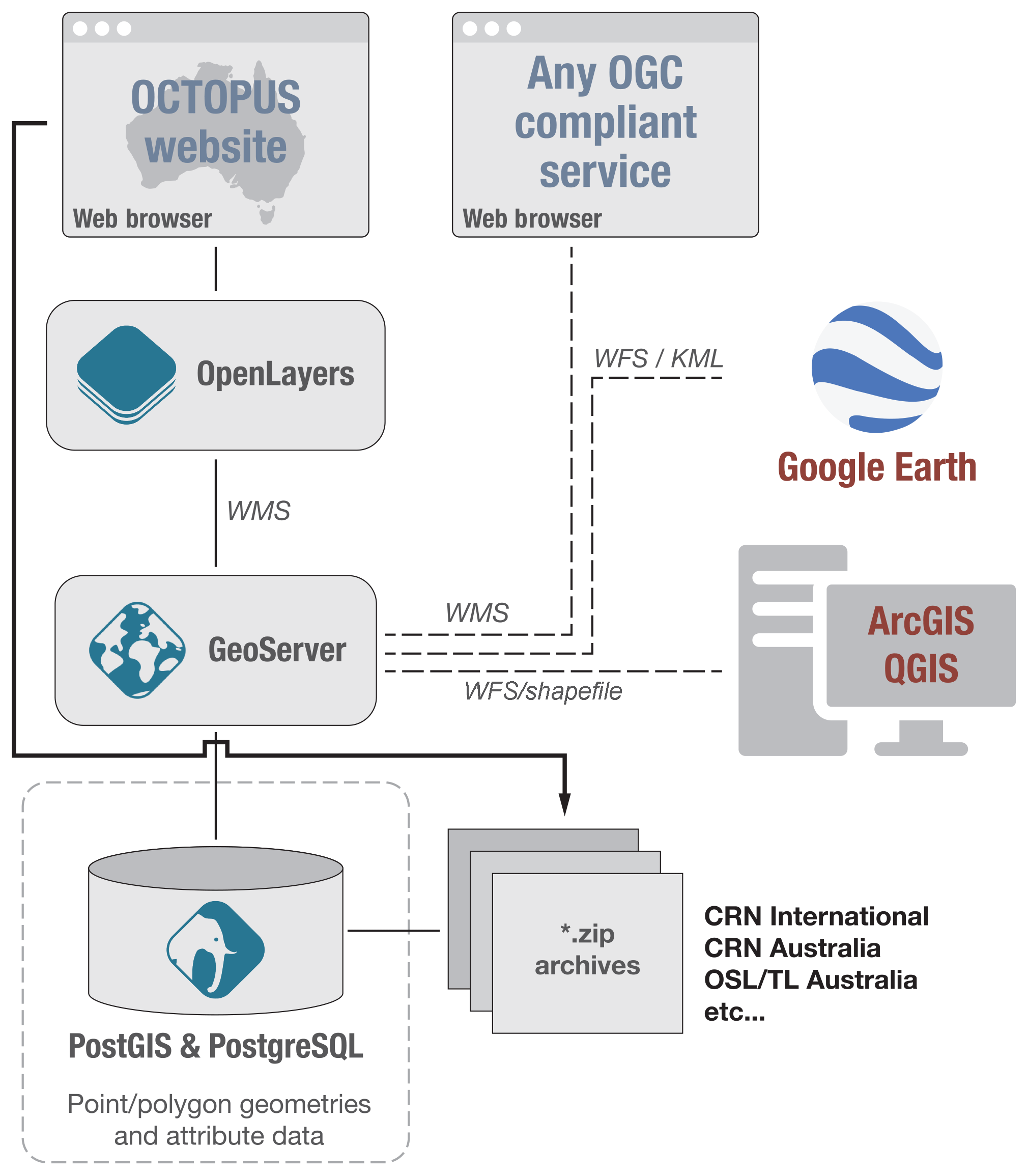
Figure 1The setup of the OCTOPUS data-storage and -sharing platform. See text for more details.
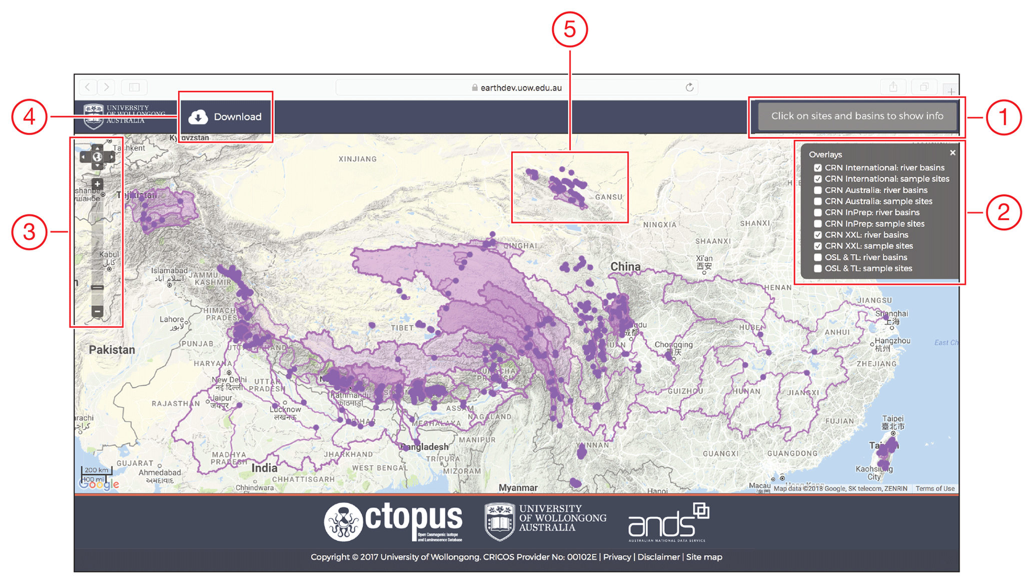
Figure 2The OCTOPUS web interface with main elements: (1) message box that provides the user with step-by-step help on how to navigate the web page, (2) collapsible panel with a list of all available data layers, (3) navigation buttons, (4) data download button, (5) Google Terrain base map and point and polygon data layers. See text for more details.
3.1 System architecture
The software architecture behind OCTOPUS is illustrated in Fig. 1. The data are stored in two separate locations. First, tabular data and the point and polygon geometries associated with each sample site or study (see Sect. 4) are stored in a PostGIS database. PostGIS (https://postgis.net, last access: 28 November 2018) is a spatial database extender for the PostgreSQL object-relational database management system (https://www.postgresql.org, last access: 28 November 2018), adding support for geographic objects and allowing location-based queries to be run in SQL. Second, all data (tabular, vector, and raster) and auxiliary information (e.g. CAIRN input and output files) (see Sect. 4) are also stored in separate zip archives, with one zip file for each study. This hybrid setup was chosen over having all tabular, vector, and raster data together in the PostGIS database because (i) it offered more flexibility regarding the list of files and file formats that could be included for download, and (ii) it made the coding of data upload and download simpler. The PostGIS database is connected to a GeoServer instance (Fig. 1). GeoServer is an open-source server that allows the sharing, processing, and editing of geospatial data (http://geoserver.org, last access: 28 November 2018), and implements a range of OCG data-sharing standards, including the widely used Web Feature Service (WFS) and the Web Map Service (WMS) standards. GeoServer also produces a variety of commonly used geospatial data formats via WFS, including KML and the ESRI Shapefile, and so can export data for using with popular desktop GIS applications such as Google Earth, ArcGIS, and QGIS (Fig. 1). It is also possible to connect to the GeoServer instance directly in QGIS and interrogate the data via the WFS protocol (see below). The OpenLayers (https://openlayers.org, last access: 28 November 2018) JavaScript library is used to display the geospatial data served by the GeoServer instance in a web browser (Fig. 1). OpenLayers also allows for the data to be queried and a selection to be made for download.
3.2 Accessing data using the web interface
The web interface has a simple design and its sole purpose is to enable users to visualise the various data collections and to select data for download. The web interface includes the following elements (Fig. 2): a message box that provides the user with step-by-step help on how to navigate the web page (Fig. 2, #1); a collapsible panel with a list of all available data layers – these are grouped by data collection (see Sect. 4) and can be toggled on or off (Fig. 2, #2); navigation buttons allowing zooming and scrolling (Fig. 2, #3); and the data download button (Fig. 2, #4). The latter opens a dialogue panel and switches the cursor from panning mode to selection mode, allowing for data layers to be selected and added to a download list. The OpenLayers map frame uses Google Terrain as the base layer and the point and polygon data are displayed using different colours for each collection (Fig. 2, #5).
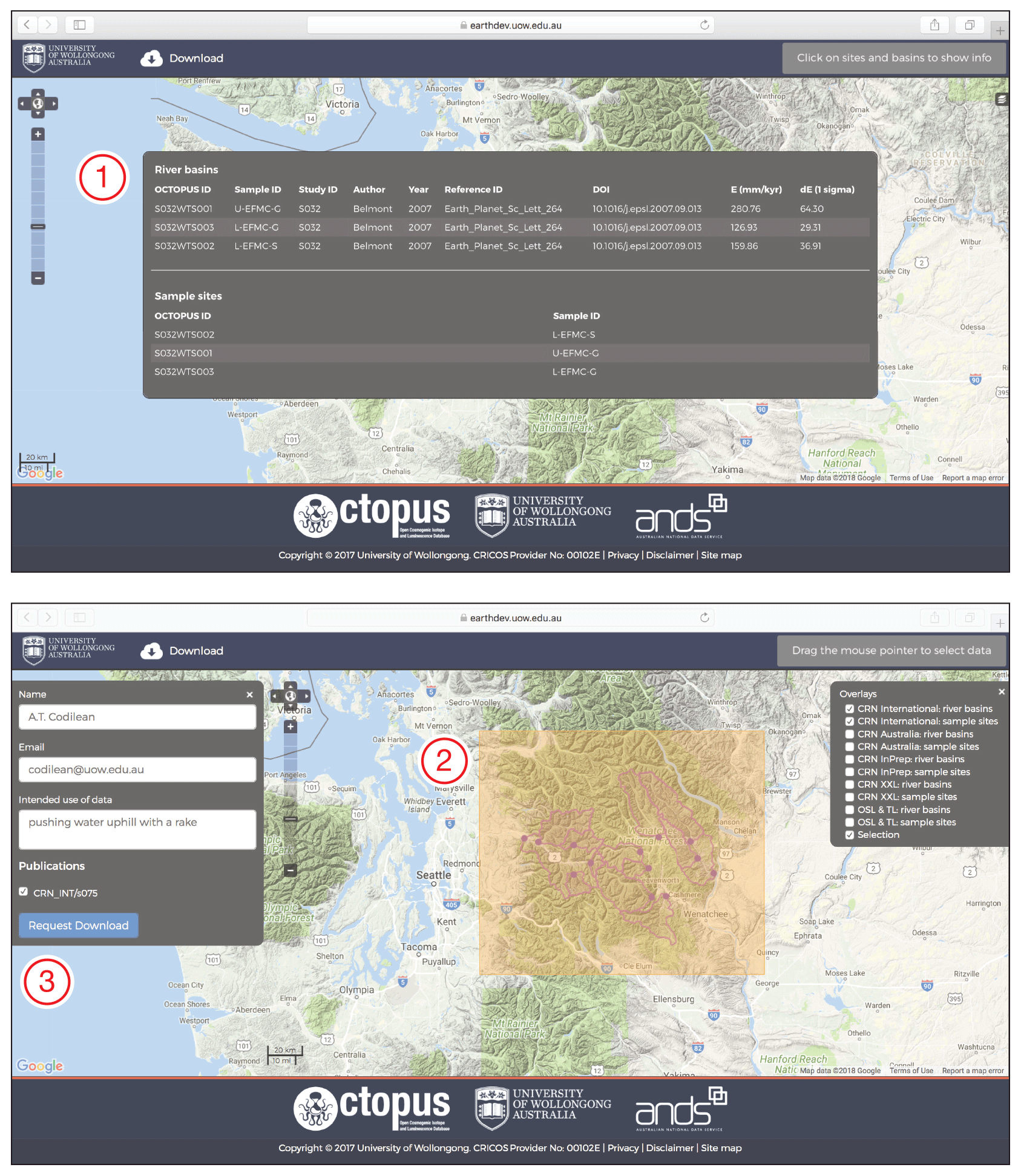
Figure 3Screenshots of the OCTOPUS web page illustrating a typical user session. See text for more details.
Figure 3 illustrates a typical user interaction with the web interface. First, the user displays the data collection(s) of interest and navigates to the desired geographical area. This can be achieved by using the navigation buttons or simply by clicking (to zoom) and dragging (to pan) on the map area. To query the data, the user clicks on a point or polygon feature. This action displays an information panel that includes a subset of the records available as part of the attribute table for each point or polygon feature. In the case of overlapping features, the information panel displays records for all features (Fig. 3, #1). Displayed information includes sample ID, publication details, and recalculated 10Be-based denudation rate with uncertainty for CRN data, or published age with uncertainty for OSL–TL data. The dialogue panel closes automatically once the user clicks anywhere outside of the panel in the map display window. The displayed data are only a subset of the available attribute data and are meant to provide the user with basic information about each point or polygon record. To download data, the user clicks on the download button. This action turns the cursor into a selection tool (the user drags a box around desired points and polygons to select) and displays a dialogue panel requesting user information such as name, email address, and the intended use of the data (Fig. 3, #2–3). The user has the option to fine-tune the list of selected studies by toggling on or off each study from the list generated after the selection box is drawn. It is possible to select multiple studies from multiple collections at the same time. A valid email address is required as links to the data are sent to the user via email immediately after the download button is pressed. There is no verification of who the data requestor is or where that person is from; however, none of the fields can be left empty and all entered information is stored in a log file permanently and is used for reporting purposes. Thus, although not mandatory, providing some meaningful information when downloading the data via the web interface will support future efforts to secure funding for OCTOPUS.
3.3 Accessing data using the Web Feature Service (WFS) capability
The web interface allows users to download all of the data: tabular, vector, and raster. The data are organised in studies – each publication is a “study” – with files belonging to each study stored in separated zip archives (see below). The size of these zip archives ranges from as small as 1 MB to just over 2.5 GB, and so the web interface is meant for downloading a small number of studies per session rather than the entire collection – the size of which at the time of writing was just over 165 GB. Users who want access to a subset or to the entire collection but who do not need access to the raster data, however, can download the tabular and vector data using the WFS capability running on the GeoServer instance, instead. WFS allows geospatial data to be interrogated and requested for download using a URL via a web browser or displayed directly in desktop applications such as QGIS (see below). It is beyond the scope of this paper to provide a manual on WFS. Rather, here we provide a series of examples that users can modify to perform basic queries and download data. For a more comprehensive introduction to WFS and GeoServer, the reader is referred to Iacovella and Youngblood (2013) or to the GeoServer documentation web page at http://docs.geoserver.org (last access: 28 November 2018).
The following example WFS request will download all drainage basins belonging to the CRN International collection in the ESRI Shapefile format:
http://earth.uow.edu.au:80/geoserver/
       wfs?request=GetFeature&typename
       =be10-denude:crn_int_basins&
       outputformat=SHAPE-ZIP
In the above example, be10-denude:crn_int_ basins
is the name of the data layer to be downloaded and SHAPE-ZIP refers to
the format used to export the data (here, ESRI Shapefile). To obtain a full list of available data layers and
export data formats, one should use the following request:
http://earth.uow.edu.au:80/geoserver/
       wfs?request=GetCapabilities
and look under FeatureTypeList and ows:OperationsMetadata in the results displayed for layer names and data formats, respectively. It is possible to request only a subset of the data by using the CQL/ECQL query language. For example, the following WFS request will download all drainage basins (with CRN data in the attribute table) from the CRN Australia collection in the ESRI Shapefile format that were published between 2005 and 2010:
http://earth.uow.edu.au:80/geoserver/
       wfs?request=GetFeature&typename
       =be10-denude:crn_aus_basins&
       outputformat=SHAPE-ZIP&
       CQL_FILTER=pubyear+BETWEEN+
       2005+AND+2010
where pubyear is the name of the field containing the publication year (see Table S1, included as part of the Supplement). Similarly, CQL_FILTER=ebe_mmkyr<10 will download all records with a 10Be denudation rate <10 mm kyr−1, and CQL_FILTER=studyid='S066' will download all records that belong to study S066. Lastly, it is also possible to subset the data by geographic location:
http://earth.uow.edu.au:80/geoserver/
       wfs?request=GetFeature&typename
       =be10-denude:crn_int_basins&
       outputformat=SHAPE-ZIP&
       BBOX=-0,20,40,60,EPSG:4326
where 0,20,40,60 are the coordinates of the bounding box used to clip the data (following the format: x1,x2,y1,y2) and EPSG:4326 indicates that the coordinates are WGS84 latitude and longitude in degrees (for a complete list of EPSG references see http://spatialreference.org, last access: 28 November 2018).
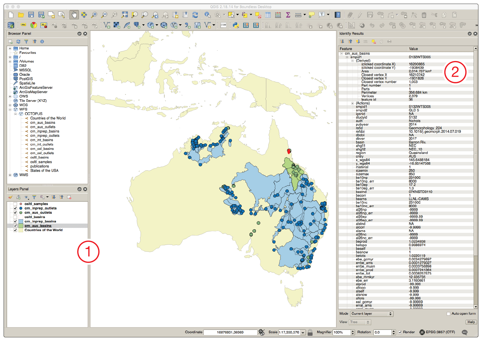
Figure 4Screenshot of the QGIS application interface displaying data from OCTOPUS accessed through a WFS connection. A WFS connection will provide direct access to the data, meaning that (1) its symbology can be modified, (2) it can be queried, and analysis functions can be run on it.
For users that wish to display and interrogate the data without actually downloading any files, it is possible to access OCTOPUS from QGIS directly by using the “add WFS layer” function and connecting to
http://earth.uow.edu.au:80/geoserver/wfs
QGIS is a free and open-source cross-platform desktop GIS application that supports viewing, editing, and analysis of geospatial data (https://www.qgis.org, last access: 28 November 2018). An example QGIS session with a WFS connection to OCTOPUS is shown in Fig. 4. A WFS connection will provide direct access to the data, and so any data accessed remotely is treated in the same way as data stored locally. Thus, it is possible to modify the symbology of the layers, query the data, and run analysis functions on them. However, all the above come at the cost of much more data being transmitted, and so users wanting to perform analyses on the OCTOPUS collections are recommended to instead download a local copy of the data first using one of the methods described above.
The compiled CRN and OSL–TL data are organised in three collections, namely (i) CRN International, including 10Be (and 26Al) measurements in fluvial sediment samples from across the globe but excluding Australia; (ii) CRN Australia, including 10Be (and 26Al) measurements in fluvial sediment samples from Australia; and (iii) OSL & TL Australia, including OSL and TL measurements in fluvial sediment samples from stratigraphic sections and sediment cores from across the Australian continent. The aim of OCTOPUS is to compile and incorporate all data – both published and unpublished – that is publicly available and we do not think that it is our role to decide on the quality of the data that is already published. However, in some instances, where a publication did not provide sufficient information for the data files to be produced (e.g, insufficient information to be able to confidently locate and delineate drainage basins) and this information could not be obtained from elsewhere, those data were excluded from OCTOPUS. Further, despite our best efforts it is likely that we have missed some studies during our search. Given the above, there are studies that were excluded from the current release of OCTOPUS. This was not an editorial decision except in cases where we had no choice due to a lack of information (see above).
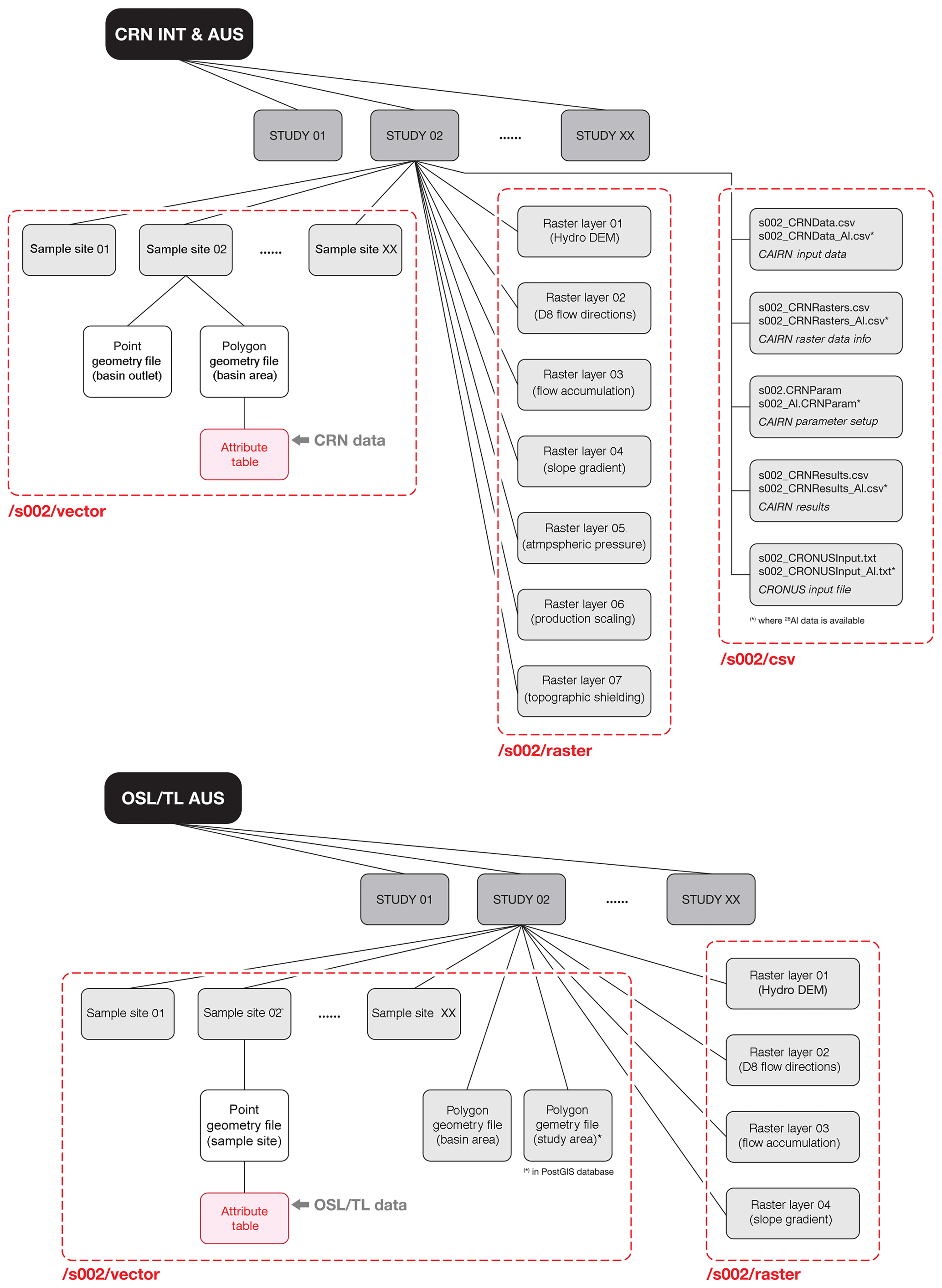
Figure 5Data organisation diagrams for the CRN and OSL–TL collections. See text for details.
4.1 CRN International and CRN Australia
The CRN International and CRN Australia collections consist of 10Be (and where available, also 26Al) basin-wide denudation rates published in the peer-reviewed literature up to 2018. As already mentioned, the data are organised in studies, with files belonging to each study stored in separated zip archives (Fig. 5). The mean sample number per study is ∼20 and the ratio of published 26Al to published 10Be measurements is approximately 1 to 10. For each 10Be data point, there is a point geometry file representing the location of the sample site, and a polygon geometry file representing the outline of the drainage basin from which the sampled material is originating. An attribute table including published and recalculated 10Be (and 26Al) data and a comprehensive set of metadata is linked to the polygon geometry file. A complete description of all attribute data entries is provided in Table S1, included as part of the Supplement. For each study, each zip archive also includes seven raster layers: (i) a hydrologically corrected DEM with elevation values in metres (file name suffix: _demhydro), (ii) a flow-direction raster calculated using the D8 flow-routing method (Jenson and Domingue, 1988) (_d8flowdir), (iii) a flow-accumulation raster calculated with the same D8 method (_flowacc), (iv) a slope gradient raster calculated using the method described in Horn (1981) with units in m km−1 (_gradmkm), (v) an atmospheric pressure raster, showing local atmospheric pressure in hPa calculated based on the NCEP2 climate reanalysis data (Compo et al., 2011) (_atmospres), (vi) a cosmogenic nuclide production scaling raster calculated using the method described in Stone (2000) (_prodscale), and (vii) a cosmogenic nuclide production topographic shielding raster calculated using the method described in Codilean (2006) (_toposhield). All raster layers were derived using the Shuttle Radar Topography Mission (SRTM) 90 m Digital Elevation Database (Farr et al., 2007) and extend 20 km beyond the boundaries of the drainage basins in each study. For two studies, namely Henck et al. (2011) and Reber et al. (2017), due to very large basin areas, all raster layers with the exception of slope gradient were calculated from SRTM data resampled to 500 m resolution. Each zip archive also includes a series of text files representing CAIRN configuration and input data files, and CAIRN output files, including files to be used with the online calculators formerly known as the CRONUS-Earth online calculators (Balco et al., 2008).
Published 10Be concentrations (atoms g−1) were renormalised to the Nishiizumi 2007 10Be AMS standard (Nishiizumi et al., 2007), and basin-wide denudation rates recalculated with CAIRN. Basin-averaged nuclide production from neutrons and muons was calculated with the approximation of Braucher et al. (2011) and using a sea-level and high-latitude total 10Be production rate of 4.3 (Mudd et al., 2016). Production rates for catchment-wide denudation rates were calculated at every pixel using the SRTM 90 m DEM, with the time-independent Lal/Stone scaling scheme (Stone, 2000). Atmospheric pressure was calculated via interpolation from the NCEP2 reanalysis data (Compo et al., 2011). Topographic shielding was calculated from the same DEM using the method of Codilean (2006) with θ=8∘ and ϕ=5∘. Following the submission of this paper, a new study by DiBiase (2018) showed that topographic shielding corrections are inappropriate for calculating basin-wide denudation rates, in most settings, and are only required for steep catchments with non-uniform distribution of quartz and/or denudation rates. For this reason, future iterations of the CRN International and CRN Australia collections will also include 10Be (and where available 26Al) denudation rates calculated without correcting for topographic shielding. All calculations assumed a 10Be half-life of 1.387±0.012 Myr (Chmeleff et al., 2010; Korschinek et al., 2010).
For simplicity and consistency across the global compilation, no corrections were made for lithological differences in quartz abundance, glacier cover, and snow shielding. Performing such corrections in a consistent manner on a global scale is impossible. However, all CAIRN input and configuration files are provided and these corrections can be readily applied by end users to individual studies. Further, CRN International and CRN Australia include both the originally published denudation rates and the ones recalculated using CAIRN, and so detailed comparisons can be made by users. Figure 6 shows a first-order comparison between published and recalculated 10Be denudation rates. With the exception of a small number of data points (n∼10), there is good agreement between published and recalculated 10Be denudation rates, with no obvious trends related to elevation or basin size. Where large discrepancies exist, these are due either to differences in drainage basins as published versus drainage basins identified on the SRTM DEM during data recalculation or due to corrections that were applied to the data in the original publication that were not appropriately described in the latter. Discrepancies also exist in the case of studies where substantial portions of a drainage basin consisted on non-quartz-bearing lithologies (e.g. Safran et al., 2005; Croke et al., 2015) and where corrections for quartz abundance were applied to the data in the original publications but were not replicated here. The number of such basins is small, however, and will not impact any regional or larger-scale analyses done with the CRN data. For small-scale studies users should compare published with recalculated denudation rates and determine whether a new recalculation that involves corrections for quartz abundance, glacier cover, and/or snow shielding is warranted.
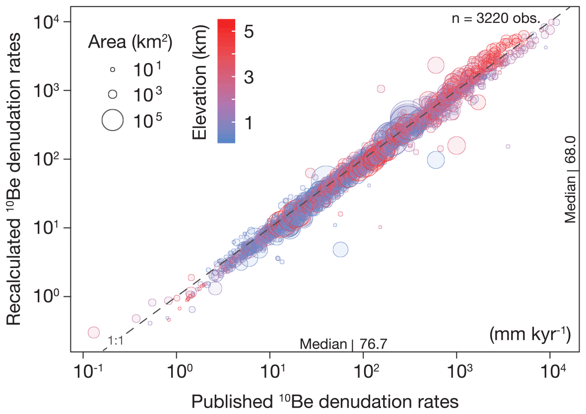
Figure 6Published versus recalculated 10Be-based denudation rates. Data points are coloured according to average basin elevation and circle sizes are proportional to basin area. Note the good agreement between the two data sets and the lack of obvious trends related to basin elevation and basin area.
Approximately 5 % of compiled 10Be measurements – all of which were published in two highly regarded journals – could not be incorporated into OCTOPUS due to information that is insufficient to reproduce drainage basin extents.
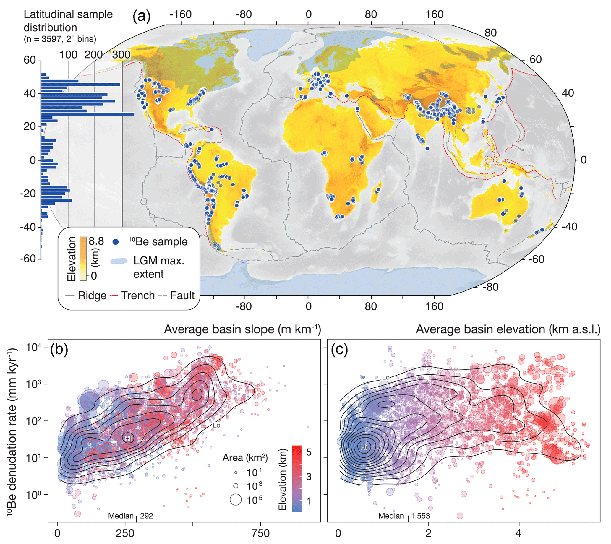
Figure 7The global CRN data set: (a) geographical extent and latitudinal sample distribution, (b) average basin slope versus recalculated 10Be denudation rate, and (c) average basin elevation versus recalculated 10Be denudation rate. Data points in (b) and (c) are coloured according to average basin elevation and circle sizes are proportional with basin area. Contour lines show kernel density estimates for the point clouds (arbitrary units).
In terms of geographical extent, the global CRN compilation exhibits considerable bias (Fig. 7a). The majority of the 10Be (and 26Al) measurements are from Northern Hemisphere drainage basins, clustering around distinct, mostly tectonically active, topographic regions, such as the Pacific coast of the United States, the Appalachians, the European Alps, and the Tibet-Himalaya region. Due to some recent studies, there is also good coverage of the South American Cordillera. However, there is a considerable lack of data from low-gradient and tectonically passive regions, such as large parts of Australia, most of Africa, and most of Asia less the Tibet-Himalaya region. Further, there are no data from latitudes above ∼55∘. The observed geographical bias is a reflection of the intense interest of the geomorphological community in estimating rates of erosion and weathering in tectonically active mountain regions with one of several aims to understand the role of surface processes in the global climate system (e.g. Molnar and England, 1990; Raymo and Ruddiman, 1992; Willenbring and von Blanckenburg, 2010; Herman et al., 2013). Further, the lack of data from high latitudes is partly due to the desire to stay away from formerly glaciated environments. Although the geographical bias does not make the CRN collection less valuable, it may confound studies aiming to infer global-scale trends from these data (cf. Portenga and Bierman, 2011; Willenbring et al., 2013; Harel et al., 2016). Despite the geographical bias, however, the global CRN data sample basins with a wide range of slope gradients, elevations, and basin areas (Fig. 7b–c).
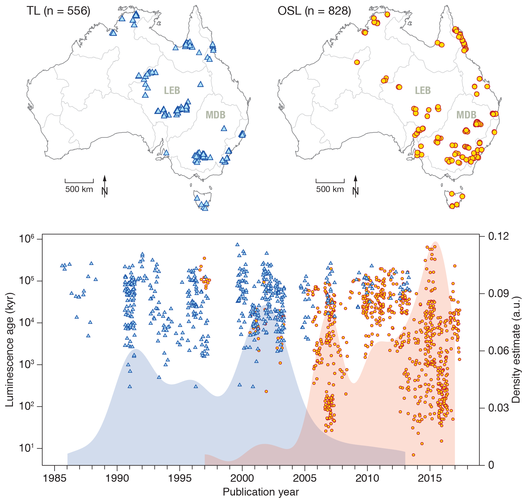
Figure 8The spatial and temporal extents of the OSL & TL Australia data set. Blue triangles denote TL measurements and yellow circles denote OSL measurements. Grey lines depict major topographic drainage divisions and river regions based on the Australian Hydrological Geospatial Fabric (Geofabric).
4.2 OSL & TL Australia
The OSL & TL Australia collection consists of thermoluminescence (TL) and optically stimulated luminescence (OSL) measurements in fluvial sediment samples from stratigraphic sections and sediment cores from across the Australian continent. The collection includes data published in the peer-reviewed literature up to 2017 and also previously unpublished data compiled from technical reports and various Honours, MSc, and PhD theses. The majority of the TL data are from sources published from 1986 up to 2005, whereas the majority of the OSL data are from sources less than 10 years old (Fig. 8). In terms of geographical extent both TL and OSL data are concentrated in the south-eastern and eastern parts of the Australian continent, with ∼500 measurements from Australia's largest river basins – Lake Eyre (LEB) and Murray-Darling (MDB) basins – and with an equal amount from rivers draining the eastern seaboard (Fig. 8). The western half of Australia is severely understudied, with one single OSL study for the entire region, namely Veth et al. (2009). Focused interest on river systems is proximal to high-population density areas, where floods are a potential threat (e.g. Brisbane River, after major floods in 2011; Croke et al., 2016), or where rivers are of great agricultural importance, such as the MDB. This well-justified bias, however, leaves a gap in the understanding of regions dominated by rivers that are now dry or ephemeral and yet that could hold information on past climatic regimes now buried under the desert sand. The focus on south-eastern coastal river systems draining the Great Dividing Range could be a source of bias in continent-wide interpretations, where the rivers draining the western intracontinental ranges and plains remain underrepresented.
Similarly to the CRN collections, the data are organised in studies – each publication is a study – with files belonging to each study stored in separated zip archives (Fig. 5). For each OSL or TL data point, there is a point geometry file representing the location of the sample site. An attribute table including published OSL or TL ages and a comprehensive set of metadata is linked to the point geometry file (a complete description of all attribute data entries is provided in Table S2, included as part of the Supplement). The zip archive also includes two separate polygon geometry files: one representing the outline of the drainage basin of the most downstream sample and one representing the area extending 20 km beyond the boundaries of this drainage basin. For studies with basin areas up to 100 000 km2, each zip archive also includes four raster layers: (i) a hydrologically corrected DEM with elevation values in m (file name suffix: _demhydro), (ii) a flow-direction raster calculated using the D8 flow-routing method (Jenson and Domingue, 1988) (_d8flowdir), (iii) a flow-accumulation raster calculated with the same D8 method (_flowacc), and (iv) a slope gradient raster calculated using the method described in Horn (1981) with units in m km−1 (_gradmkm). All raster layers were derived using the hydrologically enforced SRTM 30 m digital elevation model (DEM-H) obtained from Geoscience Australia (Geoscience Australia, 2011) and were clipped to the extent of the 20 km buffer polygon layer. For studies with basin areas exceeding 100 000 km2 (e.g. Callen and Nanson, 1992; Bourman et al., 2010; Jansen et al., 2013) raster layers (i) to (iii) were derived using Geoscience Australia's GEODATA 250 m digital elevation model and flow-direction grid (Geoscience Australia, 2008), as the SRTM DEM produced files that were too large to transfer online.
4.3 Other collections
In addition to the CRN and OSL–TL collections described above, the current version of OCTOPUS also includes additional CRN data organised under two collections: CRN XXL and CRN In-Prep. These two collections are not officially supported by the OCTOPUS project, and are included here only for completeness. The first collection consists of five studies with samples from the Yangtse (Chappell et al., 2006), Amazon (Wittmann et al., 2009, 2011), Ganga (Lupker et al., 2012), and Brahmaputra basins (Lupker et al., 2017). These studies focused on very large basins that could only be handled by CAIRN when run using a 500 m resolution DEM that, however, produced drainage basins that were substantially different to what was published, especially in the case of rivers in the Amazon basin. Further, Chappell et al. (2006) do not report denudation rates – suggesting that calculating these might have little meaning for their samples – and both Wittmann et al. (2009, 2011) and Lupker et al. (2012, 2017) perform corrections to the data, some of which (e.g. removing floodplain areas from production rate calculations) we did not wish to replicate. To this end, CRN XXL does not include recalculated values nor does it include any raster layers. CRN In-Prep is an inventory of samples processed at the University of Wollongong where 10Be and 26Al have been measured and the data are not yet published. The collection includes sample metadata and point and polygon geometry files.
User contributions to OCTOPUS are welcome. Those wishing to submit data should download a study and use that as the template for data structure, formats, and naming convention (see also Fig. 5). As a minimum, a contribution should include point and polygon geometry files, and an attribute table with all records listed in Tables S1 and S2 with the exception of those records that are output by CAIRN. Data files should be submitted to the contact address listed in the email received from OCTOPUS when downloading data. The data collections making up OCTOPUS have been assigned digital object identifiers (DOIs), and as a consequence, adding new data needs to follow a versioning scheme, with each new version requiring new DOIs. Thus, data contributed by users will be incorporated in the next release of a given collection, rather than being added to the current one.
OCTOPUS can be accessed at https://earth.uow.edu.au (last access: 28 November 2018). The data collections that make up the 2018 release of OCTOPUS (version 1 – Dooku's Dilemma) have been assigned the following DOIs: https://doi.org/10.4225/48/5a8367feac9b2 (CRN International; Codilean et al., 2017a), https://doi.org/10.4225/48/5a836cdfac9b5 (CRN Australia; Codilean et al., 2017b), and https://doi.org/10.4225/48/5a836db1ac9b6 (OSL & TL Australia; Codilean et al., 2017c). A copy of OCTOPUS has also been deployed to https://earthtest.uow.edu.au (last access: 28 November 2018). This copy is not supported and is used for testing modifications to the website and data collections before deployment to the official site. Users should refer to the DOIs provided to ensure that they are accessing the current and supported version of the data.
We have produced a database of cosmogenic radionuclide and luminescence measurements in fluvial sediment and we have built infrastructure for hosting and maintaining the data at the University of Wollongong and making them available to the research community via an Open Geospatial Consortium (OGC)-compliant web service. The database consists of 10Be, 26Al, TL, and OSL measurements in fluvial sediment samples along with ancillary geospatial vector and raster layers. Sample metadata are comprehensive and include all necessary information for the recalculation of 10Be and 26Al denudation rates using the CAIRN program. The repository and visualisation system enable easy search and discovery of available data. Use of open standards also ensures that data layers are visible to other OGC-compliant data-sharing services. Thus, this project will turn data that were previously invisible to those not within the CRN and luminescence research community into a findable resource. This aspect is of particular importance to industry or local government who are yet to discover the value of geochronological data, for example, in evaluating how human-induced land use practices have accelerated soil erosion and which measures are necessary for restoring these rates to their natural benchmark levels. Our intention is for OCTOPUS to become the default go-to place for CRN and luminescence data. The availability of the repository and its associated data curation framework will provide the opportunity for researchers to store, curate, recalculate and reuse previously published but otherwise unusable CRN and luminescence data. This delivers the potential to harness old but valuable data that would otherwise be lost to the research community. OCTOPUS will enable new research and generate new knowledge by converting a multitude of disconnected data sets into one connected and streamlined database. Current data sets allow local-scale analyses. The streamlined database will allow for regional-scale and even continental- or global-scale analyses. The transparent data reanalysis framework will also reduce research time and avoid the duplication of effort, which will be highly attractive to other researchers. Ultimately, OCTOPUS will ensure that CRN and luminescence data are reusable beyond the scope of the project for which they were initially collected.
The supplement related to this article is available online at: https://doi.org/10.5194/essd-10-2123-2018-supplement.
ATC, HM, TJC, and WMS compiled the CRN and luminescence data; ATC and HM performed the GIS analyses and the data recalculations using CAIRN with input from SMM; AG designed and built the OCTOPUS platform and web interface with input from ATC. All authors contributed to the writing of the manuscript.
The authors declare that they have no conflict of interest.
We acknowledge financial support from the Australian National Data Service
(ANDS – Project HVC15) and the University of Wollongong (UOW) to
Alexandru T. Codilean and Timothy J. Cohen. Henry Munack benefited from an
Endeavour Postdoctoral Research Fellowship granted by the Australian
Government. A prototype of OCTOPUS was built while Alexandru T. Codilean
worked at the Deutsches GeoForschungsZentrum (GFZ). We thank Monika Oakman,
Ben Cornwell, Peter Newnam, Clare Job, Gabriel Enge, Heidi Brown,
Alan Glixman, and Keith Russell for their support during this project. We
also thank the CRN and luminescence communities for generously sharing their
data. We thank Greg Balco, Zsófia Ruszkiczay-Rüdiger,
Sebastian Kreutzer, and István Gábor Hatvani for careful reviews of
the discussion paper. We also thank Ingrid Ward, Todd Ehlers, and
Vincent Godard for providing comments on the discussion
paper.
Edited by: Attila Demény
Reviewed by: Greg
Balco, Sebastian Kreutzer, Zsófia Ruszkiczay-Rüdiger, and István
Gábor Hatvani
Aitken, M. J.: Thermoluminescence dating, Academic Press, London, 1985. a
Aitken, M. J.: An Introduction to Optical Dating, Oxford University Press, Oxford, 1998. a
Argento, D. C., Stone, J. O., Reedy, R. C., and O'Brien, K.: Physics-based modeling of cosmogenic nuclides part I: Radiation transport methods and new insights, Quat. Geochronol., 26, 29–43, https://doi.org/10.1016/j.quageo.2014.09.004, 2015a. a
Argento, D. C., Stone, J. O., Reedy, R. C., and O'Brien, K.: Physics-based modeling of cosmogenic nuclides part II: Key aspects of in-situ cosmogenic nuclide production, Quat. Geochronol., 26, 44–55, https://doi.org/10.1016/j.quageo.2014.09.005, 2015b. a
Arnold, L. J., Demuro, M., Parés, J. M., Pérez-González, A., Arsuaga, J. L., de Castro, J. M. B., and Carbonell, E.: Evaluating the suitability of extended-range luminescence dating techniques over early and Middle Pleistocene timescales: Published datasets and case studies from Atapuerca, Spain, Quaternary Int., 389, 167–190, https://doi.org/10.1016/j.quaint.2014.08.010, 2015. a
Balco, G.: Contributions and unrealized potential contributions of cosmogenic-nuclide exposure dating to glacier chronology, 1990–2010, Quaternary Sci. Rev., 30, 3–27, https://doi.org/10.1016/j.quascirev.2010.11.003, 2011. a
Balco, G., Stone, J. O., Lifton, N. A., and Dunai, T. J.: A complete and easily accessible means of calculating surface exposure ages or erosion rates from 10Be and 26Al measurements, Quat. Geochronol., 3, 174–195, https://doi.org/10.1016/j.quageo.2007.12.001, 2008. a, b, c
Bierman, P. R. and Nichols, K. K.: Rock to sediment – slope to sea with 10Be – rates of landscape change, Annu. Rev. Earth Pl. Sc., 32, 215–255, https://doi.org/10.1146/annurev.earth.32.101802.120539, 2004. a
Bierman, P. R. and Steig, E.: Estimating rates of denudation using cosmogenic isotope abundances in sediment, Earth Surf. Proc. Land., 21, 125–139, https://doi.org/10.1002/(SICI)1096-9837(199602)21:2<125::AID-ESP511>3.0.CO;2-8, 1996. a
Borchers, B., Marrero, S., Balco, G., Caffee, M. W., Goehring, B. M., Lifton, N. A., Nishiizumi, K., Phillips, F., Schaefer, J. M., and Stone, J. O.: Geological calibration of spallation production rates in the CRONUS-Earth project, Quat. Geochronol., 31, 188–198, https://doi.org/10.1016/j.quageo.2015.01.009, 2015. a
Bourman, R. P., Prescott, J. R., Banerjee, D., Alley, N. F., and Buckman, S.: Age and origin of alluvial sediments within and flanking the Mt Lofty Ranges, southern South Australia: a Late Quaternary archive of climate and environmental change, Aust. J. Earth Sci., 57, 175–192, https://doi.org/10.1080/08120090903416260, 2010. a
Braucher, R., Merchel, S., Borgomano, J., and Bourles, D. L.: Production of cosmogenic radionuclides at great depth: A multi element approach, Earth Planet. Sc. Lett., 309, 1–9, https://doi.org/10.1016/j.epsl.2011.06.036, 2011. a
Bristow, C., Augustinus, P., Wallis, I., Jol, H., and Rhodes, E.: Investigation of the age and migration of reversing dunes in Antarctica using GPR and OSL, with implications for GPR on Mars, Earth Planet. Sc. Lett., 289, 30–42, https://doi.org/10.1016/j.epsl.2009.10.026, 2010. a
Brown, E., Stallard, R., Larsen, M. C., Raisbeck, G., and Yiou, F.: Denudation Rates Determined From the Accumulation of In Situ-Produced 10Be in the Luquillo Experimental Forest, Puerto-Rico, Earth Planet. Sc. Lett., 129, 193–202, https://doi.org/10.1016/0012-821X(94)00249-X, 1995. a
Callen, R. and Nanson, G.: Formation and age of dunes in the Lake Eyre Depocentres, Geol. Rundsch., 81, 589–593, https://doi.org/10.1007/BF01828619, 1992. a
Chappell, J., Zheng, H., and Fifield, K.: Yangtse River sediments and erosion rates from source to sink traced with cosmogenic 10Be: Sediments from major rivers, Palaeogeogr. Palaeocl., 241, 79–94, https://doi.org/10.1016/j.palaeo.2006.06.010, 2006. a, b
Chmeleff, J., von Blanckenburg, F., Kossert, K., and Jakob, D.: Determination of the 10Be half-life by multicollector ICP-MS and liquid scintillation counting, Nucl. Instrum. Meth. B, 268, 192–199, https://doi.org/10.1016/j.nimb.2009.09.012, 2010. a, b
Codilean, A. T.: Calculation of the cosmogenic nuclide production topographic shielding scaling factor for large areas using DEMs, Earth Surf. Proc. Land., 31, 785–794, https://doi.org/10.1002/esp.1336, 2006. a, b, c
Codilean, A. T., Cohen, T. J., and Munack, H.: OCTOPUS –CRN International, https://doi.org/10.4225/48/5a8367feac9b2, 2017a. a
Codilean, A. T., Cohen, T. J., and Munack, H.: OCTOPUS – CRN Australia, https://doi.org/10.4225/48/5a836cdfac9b5, 2017b. a
Codilean, A. T., Cohen, T. J., Munack, H., and Saktura, W. M.: OCTOPUS – OSL/TL Australia, https://doi.org/10.4225/48/5a836db1ac9b6, 2017c. a
Compo, G. P., Whitaker, J. S., Sardeshmukh, P. D., Matsui, N., Allan, R. J., Yin, X., Gleason, B. E., Vose, R. S., Rutledge, G., Bessemoulin, P., Brönnimann, S., Brunet, M., Crouthamel, R. I., Grant, A. N., Groisman, P. Y., Jones, P. D., Kruk, M. C., Kruger, A. C., Marshall, G. J., Maugeri, M., Mok, H. Y., Nordli, O., Ross, T. F., Trigo, R. M., Wang, X. L., Woodruff, S. D., and Worley, S. J.: The Twentieth Century Reanalysis Project, Q. J. Roy. Meteor. Soc., 137, 1–28, https://doi.org/10.1002/qj.776, 2011. a, b
Croke, J., Bartley, R., Chappell, J., Austin, J. M., Fifield, K., Tims, S. G., Thompson, C. J., and Furuichi, T.: 10Be-derived denudation rates from the Burdekin catchment: The largest contributor of sediment to the Great Barrier Reef, Geomorphology, 241, 122–134, https://doi.org/10.1016/j.geomorph.2015.04.003, 2015. a
Croke, J., Thompson, C., Denham, R., Haines, H., Sharma, A., and Pietsch, T.: Reconstructing a millennial-scale record of flooding in a single valley setting: the 2011 flood-affected Lockyer Valley, south-east Queensland, Australia, J. Quaternary Sci., 31, 936–952, https://doi.org/10.1002/jqs.2919, 2016. a, b
DiBiase, R. A.: Short communication: Increasing vertical attenuation length of cosmogenic nuclide production on steep slopes negates topographic shielding corrections for catchment erosion rates, Earth Surf. Dynam., 6, 923–931, https://doi.org/10.5194/esurf-6-923-2018, 2018. a, b
Dunai, T. J.: Cosmogenic Nuclides: Principles, concepts and applications in the Earth surface sciences, Cambridge University Press, Cambridge, 2010. a, b
Dunai, T. J. and Stuart, F. M.: Reporting of cosmogenic nuclide data for exposure age and erosion rate determinations, Quat. Geochronol., 4, 437–440, https://doi.org/10.1016/j.quageo.2009.04.003, 2009. a
Dunne, J., Elmore, D., and Muzikar, P.: Scaling factors for the rates of production of cosmogenic nuclides for geometric shielding and attenuation at depth on sloped surfaces, Geomorphology, 27, 3–11, https://doi.org/10.1016/S0169-555X(98)00086-5, 1999. a
Farr, T. G., Rosen, P. A., Caro, E., Crippen, R., Duren, R., Hensley, S., Kobrick, M., Paller, M., Rodriguez, E., Roth, L., Seal, D., Shaffer, S., Shimada, J., Umland, J., Werner, M., Oskin, M., Burbank, D., and Alsdorf, D.: The Shuttle Radar Topography Mission, Rev. Geophys., 45, RG2004, https://doi.org/10.1029/2005RG000183, 2007. a
Fitzsimmons, K. E., Rhodes, E. J., Magee, J. W., and Barrows, T. T.: The timing of linear dune activity in the Strzelecki and Tirari Deserts, Australia, Quaternary Sci. Rev., 26, 2598–2616, https://doi.org/10.1016/j.quascirev.2007.06.010, 2007. a
Frankel, K. L., Finkel, R. C., and Owen, L.: Terrestrial Cosmogenic Nuclide Geochronology Data Reporting Standards Needed, Eos T. Am. Geophys. Un., 91, 31–32, https://doi.org/10.1029/2010EO040003, 2010. a
Fuchs, M. and Owen, L. A.: Luminescence dating of glacial and associated sediments: review, recommendations and future directions, Boreas, 37, 636–659, https://doi.org/10.1111/j.1502-3885.2008.00052.x, 2008. a
Fujioka, T., Chappell, J., Fifield, L. K., and Rhodes, E. J.: Australian desert dune fields initiated with Pliocene–Pleistocene global climatic shift, Geology, 37, 51–54, https://doi.org/10.1130/G25042A.1, 2009. a
Galbraith, R. F., Roberts, R. G., Laslett, G. M., Yoshida, H., and Olley, J. M.: Optical dating of single and multiple grains of quartz from Jinmium rock shelter, northern Australia: Part I, experimental design and statistical models, Archaeometry, 41, 339–364, https://doi.org/10.1111/j.1475-4754.1999.tb00987.x, 1999. a
Geoscience Australia: GEODATA 9 second DEM and D8: Digital Elevation Model Version 3 and Flow Direction Grid 2008. Bioregional Assessment Source Dataset, available at: http://data.bioregionalassessments.gov.au/dataset/ebcf6ca2-513a-4ec7-9323-73508c5d7b93 (last access: 28 November 2018), 2008. a
Geoscience Australia: Geoscience Australia, 1 second SRTM Digital Elevation Model (DEM), Bioregional Assessment Source Dataset, available at: http://data.bioregionalassessments.gov.au/dataset/9a9284b6-eb45-4a13-97d0-91bf25f1187b (last access: 28 November 2018), 2011. a
Granger, D. E. and Schaller, M.: Cosmogenic Nuclides and Erosion at the Watershed Scale, Elements, 10, 369–373, https://doi.org/10.2113/gselements.10.5.369, 2014. a, b, c
Granger, D. E., Kirchner, J. W., and Finkel, R. C.: Spatially averaged long-term erosion rates measured from in situ-produced cosmogenic nuclides in alluvial sediment, J. Geol., 104, 249–257, 1996. a
Granger, D. E., Lifton, N. A., and Willenbring, J. K.: A cosmic trip: 25 years of cosmogenic nuclides in geology, Geol. Soc. Am. Bull., 125, 1379, https://doi.org/10.1130/B30774.1, 2013. a, b, c
Harel, M. A., Mudd, S. M., and Attal, M.: Global analysis of the stream power law parameters based on worldwide 10Be denudation rates, Geomorphology, 268, 184–196, https://doi.org/10.1016/j.geomorph.2016.05.035, 2016. a
Henck, A. C., Huntington, K. W., Stone, J. O., Montgomery, D. R., and Hallet, B.: Spatial controls on erosion in the Three Rivers Region, southeastern Tibet and southwestern China, Earth Planet. Sc. Lett., 303, 71–83, https://doi.org/10.1016/j.epsl.2010.12.038, 2011. a
Herman, F., Seward, D., Valla, P. G., Carter, A., Kohn, B., Willett, S. D., and Ehlers, T. A.: Worldwide acceleration of mountain erosion under a cooling climate, Nature, 504, 423–426, https://doi.org/10.1038/nature12877, 2013. a
Horn, B. K. P.: Hill shading and the reflectance map, P. IEEE, 69, 14–47, 1981. a, b
Huntley, D. J., Godfrey-Smith, D. I., and Thewalt, M. L. W.: Optical dating of sediments, Nature, 313, 105–107, https://doi.org/10.1038/313105a0, 1985. a
Iacovella, S. and Youngblood, B.: GeoServer Beginner's Guide, Packt Publishing, Birmingham, 2013. a
Ivy-Ochs, S. and Briner, J. P.: Dating Disappearing Ice with Cosmogenic Nuclides, Elements, 10, 351–356, https://doi.org/10.2113/gselements.10.5.351, 2014. a
Jansen, J., Nanson, G., Cohen, T., Fujioka, T., Fabel, D., Larsen, J., Codilean, A., Price, D., Bowman, H., May, J.-H., and Gliganic, L.: Lowland river responses to intraplate tectonism and climate forcing quantified with luminescence and cosmogenic 10Be, Earth Planet Sc. Lett., 366, 49–58, https://doi.org/10.1016/j.epsl.2013.02.007, 2013. a
Jenson, S. K. and Domingue, J. O.: Extracting topographic structure from digital elevation data for geographic information system analysis, Photogramm. Eng. Rem. S., 54, 1593–1600, 1988. a, b
Korschinek, G., Bergmaier, A., Faestermann, T., Gerstmann, U. C., Knie, K., Rugel, G., Wallner, A., Dillmann, I., Dollinger, G., von Gostomski, C. L., Kossert, K., Maiti, M., Poutivtsev, M., and Remmert, A.: A new value for the half-life of 10Be by Heavy-Ion Elastic Recoil Detection and liquid scintillation counting, Nucl. Instrum. Meth. B, 268, 187–191, https://doi.org/10.1016/j.nimb.2009.09.020, 2010. a, b
Lal, D.: Cosmic ray labeling of erosion surfaces: in situ nuclide production rates and erosion models, Earth Planet. Sc. Lett., 104, 424–439, https://doi.org/10.1016/0012-821X(91)90220-C, 1991. a
Lewis, C. J., McDonald, E. V., Sancho, C., Peña, J. L., and Rhodes, E. J.: Climatic implications of correlated Upper Pleistocene glacial and fluvial deposits on the Cinca and Gállego Rivers (NE Spain) based on OSL dating and soil stratigraphy, Global Planet. Change, 67, 141–152, https://doi.org/10.1016/j.gloplacha.2009.01.001, 2009. a
Lifton, N. A., Sato, T., and Dunai, T. J.: Scaling in situ cosmogenic nuclide production rates using analytical approximations to atmospheric cosmic-ray fluxes, Earth Planet. Sc. Lett., 386, 149–160, https://doi.org/10.1016/j.epsl.2013.10.052, 2014. a
Lupker, M., Blard, P.-H., Lavé, J., France-Lanord, C., Leanni, L., Puchol, N., Charreau, J., and Bourlès, D.: 10Be-derived Himalayan denudation rates and sediment budgets in the Ganga basin, Earth Planet. Sc. Lett, 333–334, 146–156, https://doi.org/10.1016/j.epsl.2012.04.020, 2012. a, b
Lupker, M., Lavé, J., France-Lanord, C., Christl, M., Bourlès, D., Carcaillet, J., Maden, C., Wieler, R., Rahman, M., Bezbaruah, D., and Xiaohan, L.: 10Be systematics in the Tsangpo-Brahmaputra catchment: the cosmogenic nuclide legacy of the eastern Himalayan syntaxis, Earth Surf. Dynam., 5, 429–449, https://doi.org/10.5194/esurf-5-429-2017, 2017. a, b
Molnar, P. and England, P.: Late Cenozoic Uplift of Mountain-Ranges and Global Climate Change – Chicken or Egg, Nature, 346, 29–34, https://doi.org/10.1038/346029a0, 1990. a
Mudd, S. M., Harel, M.-A., Hurst, M. D., Grieve, S. W. D., and Marrero, S. M.: The CAIRN method: automated, reproducible calculation of catchment-averaged denudation rates from cosmogenic nuclide concentrations, Earth Surf. Dynam., 4, 655–674, https://doi.org/10.5194/esurf-4-655-2016, 2016. a, b, c
Nishiizumi, K., Imamura, M., Caffee, M. W., Southon, J. R., Finkel, R. C., and Mcaninch, J.: Absolute calibration of 10Be AMS standards, Nucl. Instrum. Meth. B, 258, 403–413, https://doi.org/10.1016/j.nimb.2007.01.297, 2007. a
Olley, J., Deckker, P. D., Roberts, R., Fifield, L., Yoshida, H., and Hancock, G.: Optical dating of deep-sea sediments using single grains of quartz: a comparison with radiocarbon, Sediment. Geol., 169, 175–189, https://doi.org/10.1016/j.sedgeo.2004.05.005, 2004. a
Pietsch, T., Brooks, A., Spencer, J., Olley, J., and Borombovits, D.: Age, distribution, and significance within a sediment budget, of in-channel depositional surfaces in the Normanby River, Queensland, Australia, Geomorphology, 239, 17–40, https://doi.org/10.1016/j.geomorph.2015.01.038, 2015. a
Portenga, E. W. and Bierman, P. R.: Understanding Earth's eroding surface with 10Be, GSA Today, 21, 4–10, https://doi.org/10.1130/G111A.1, 2011. a
Raymo, M. E. and Ruddiman, W. F.: Tectonic Forcing of Late Cenozoic Climate, Nature, 359, 117–122, https://doi.org/10.1038/359117a0, 1992. a
Reber, R., Delunel, R., Schlunegger, F., Litty, C., Madella, A., Akçar, N., and Christl, M.: Environmental controls on 10Be-based catchment-averaged denudation rates along the western margin of the Peruvian Andes, Terra Nova, 29, 282–293, https://doi.org/10.1111/ter.12274, 2017. a
Rhodes, E. and Bailey, R.: The effect of thermal transfer on the zeroing of the luminescence of quartz from recent glaciofluvial sediments, Quaternary Sci. Rev., 16, 291–298, https://doi.org/10.1016/S0277-3791(96)00100-X, 1997. a
Rhodes, E. J.: Optically Stimulated Luminescence Dating of Sediments over the Past 200,000 Years, Annu. Rev. Earth Planet. Sc., 39, 461–488, https://doi.org/10.1146/annurev-earth-040610-133425, 2011. a, b
Richards, B. W., Benn, D. I., Owen, L. A., Rhodes, E. J., and Spencer, J. Q.: Timing of late Quaternary glaciations south of Mount Everest in the Khumbu Himal, Nepal, Geol. Soc. Am. Bull., 112, 1621–1632, https://doi.org/10.1130/0016-7606(2000)112<1621:TOLQGS>2.0.CO;2, 2000. a
Rustomji, P. and Pietsch, T.: Alluvial sedimentation rates from southeastern Australia indicate post-European settlement landscape recovery, Geomorphology, 90, 73–90, https://doi.org/10.1016/j.geomorph.2007.01.009, 2007. a
Safran, E. B., Bierman, P. R., Aalto, R., Dunne, T., Whipple, K. X., and Caffee, M.: Erosion rates driven by channel network incision in the Bolivian Andes, Earth Surf. Proc. Land., 30, 1007–1024, https://doi.org/10.1002/esp.1259, 2005. a
Schaefer, J. M., Denton, G. H., Kaplan, M. R., Putnam, A., Finkel, R. C., Barrell, D. J. A., Andersen, B. G., Schwartz, R., Mackintosh, A., Chinn, T., and Schluechter, C.: High-Frequency Holocene Glacier Fluctuations in New Zealand Differ from the Northern Signature, Science, 324, 622–625, 2009. a
Schaller, M., von Blanckenburg, F., Hovius, N., Veldkamp, A., van den Berg, M., and Kubik, P. W.: Paleoerosion Rates from Cosmogenic 10Be in a 1.3 Ma Terrace Sequence: Response of the River Meuse to Changes in Climate and Rock Uplift, J. Geol., 112, 127–144, https://doi.org/10.1086/381654, 2004. a
Singarayer, J., Bailey, R., Ward, S., and Stokes, S.: Assessing the completeness of optical resetting of quartz OSL in the natural environment, Radiat. Meas., 40, 13–25, https://doi.org/10.1016/j.radmeas.2005.02.005, 2005. a
Spencer, J. Q. and Owen, L. A.: Optically stimulated luminescence dating of Late Quaternary glaciogenic sediments in the upper Hunza valley: validating the timing of glaciation and assessing dating methods, Quaternary Sci. Rev., 23, 175–191, https://doi.org/10.1016/S0277-3791(03)00220-8, 2004. a
Stone, J. O.: Air pressure and cosmogenic isotope production, J. Geophys. Res.-Sol. Ea., 105, 23753–23759, https://doi.org/10.1029/2000JB900181, 2000. a, b
Vermeesch, P.: CosmoCalc: An Excel add-in for cosmogenic nuclide calculations, Geochem. Geophy. Geosy., 8, Q08003, https://doi.org/10.1029/2006GC001530, 2007. a
Veth, P., Smith, M., Bowler, J., Fitzsimmons, K., Williams, A., and Hiscock, P.: Excavations At Parnkupirti, Lake Gregory, Great Sandy Desert: OSL Ages for Occupation before the Last Glacial Maximum, Australian Archaeology, 69, 1–10, https://doi.org/10.1080/03122417.2009.11681896, 2009. a
von Blanckenburg, F.: The control mechanisms of erosion and weathering at basin scale from cosmogenic nuclides in river sediment, Earth Planet. Sc. Lett., 237, 462–479, https://doi.org/10.1016/j.epsl.2005.06.030, 2005. a, b, c
von Blanckenburg, F. and Willenbring, J. K.: Cosmogenic Nuclides: Dates and Rates of Earth-Surface Change, Elements, 10, 341–346, https://doi.org/10.2113/gselements.10.5.341, 2014. a
Wallinga, J., Hobo, N., Cunningham, A. C., Versendaal, A. J., Makaske, B., and Middelkoop, H.: Sedimentation rates on embanked floodplains determined through quartz optical dating, Quat. Geochronol., 5, 170–175, https://doi.org/10.1016/j.quageo.2009.01.002, 2010. a
Willenbring, J. K. and von Blanckenburg, F.: Long-term stability of global erosion rates and weathering during late-Cenozoic cooling, Nature, 465, 211–214, https://doi.org/10.1038/nature09044, 2010. a
Willenbring, J. K., Codilean, A. T., and McElroy, B.: Earth is (mostly) flat: Apportionment of the flux of continental sediment over millennial time scales, Geology, 41, 343–346, https://doi.org/10.1130/G33918.1, 2013. a
Wintle, A. G.: Luminescence dating: where it has been and where it is going, Boreas, 37, 471–482, https://doi.org/10.1111/j.1502-3885.2008.00059.x, 2008. a
Wittmann, H., von Blanckenburg, F., Guyot, J., Maurice, L., and Kubik, P.: From source to sink: Preserving the cosmogenic 10Be-derived denudation rate signal of the Bolivian Andes in sediment of the Beni and Mamoré foreland basins, Earth Planet. Sc. Lett., 288, 463–474, https://doi.org/10.1016/j.epsl.2009.10.008, 2009. a, b
Wittmann, H., von Blanckenburg, F., Maurice, L., Guyot, J.-L., Filizola, N., and Kubik, P. W.: Sediment production and delivery in the Amazon River basin quantified by in situ-produced cosmogenic nuclides and recent river loads, Geol. Soc. Am. Bull., 123, 934–950, https://doi.org/10.1130/B30317.1, 2011. a, b
Wolfe, S. A., Huntley, D. J., and Ollerhead, J.: Recent and late Holocene sand dune activity in southwestern Saskatchewan, Current Research, Geological Survey of Canada, 1995-B, 131–140, 1995. a