OpenLandMap-soildb: global soil information at 30 m spatial resolution for 2000–2022+ based on spatiotemporal Machine Learning and harmonized legacy soil samples and observations

There is increasing interest in global dynamic soil information with changes in soil properties mapped over time and at high spatial resolution. Thanks to long-term, multi-temporal, and fine- and medium-resolution satellite missions such as Landsat, MODIS, Copernicus Sentinel and similar, it is possible to produce globally consistent predictions of key soil variables that match other 10–30 m spatial resolution global data sets. This paper describes data preparation, modeling, and production of OpenLandMap-soildb: global dynamic predictions of soil organic carbon content, soil organic carbon density, bulk density, soil pH in H₂O, soil texture fractions (clay, sand and silt) and USDA subgroup soil types (USDA soil taxonomy subgroups) at 30 m spatial resolution based on spatiotemporal Machine Learning (Quantile Regression Random Forest with output predictions showing the mean plus the 68 % probability lower and upper prediction intervals). To train the models, a large compilation of soil samples imported from legacy soil projects was used: 216 000 soil samples with soil carbon density (kg m⁻³), 408 000 soil samples with soil carbon content (g kg⁻¹), 272 000 soil samples with soil pH in H₂O, 363 000 soil samples with clay, silt and sand content (%) and 134 000 samples with bulk density oven dry (t m⁻³). Soil carbon and soil pH were mapped with 5-year time-intervals; soil texture fractions, bulk density, and soil types were mapped for recent years only. The cross-validation results indicate Root Mean Square Error (RMSE) of 17.7 (kg m⁻³; 0.486 in log-scale) and Concordance Correlation Coefficient (CCC) of 0.88 for SOC density, RMSE of 51.3 (g kg⁻¹; 0.574 in log-scale) and CCC of 0.87 for SOC content, RMSE of 0.15 (t m⁻³) and CCC of 0.92 for bulk density of fine-earth, RMSE of 0.51 and CCC of 0.91 for soil pH, RMSE of 8.4 % and CCC of 0.87 for soil clay content, and RMSE of 12.6 % and CCC of 0.84 for soil sand content respectively. The most important variables for predicting soil organic carbon density (kg m⁻³) were: soil depth, Landsat-based uncalibrated Gross Primary Productivity (GPP), Normalized Difference Vegetation Index (NDVI) and CHELSA bioclimatic indices. The global distribution of soil pH can be primarily explained by the CHELSA Aridity Index (long-term), annual precipitation, and salinity grade. The global stocks for 2020–2022+ period for 0–30 cm depth interval are estimated at 461 Pg (Peta grams); the results further indicate that, in the last 25 years, the world has lost at least 11 Pg of SOC in the top soil. Suggestions are made on how to set up global permanent monitoring stations to accurately track land degradation and enable land restoration projects. The training data set is available at https://doi.org/10.5281/zenodo.4748499 (Hengl and Gupta, 2025), while the resulting data products can be accessed at https://doi.org/10.5281/zenodo.15470431 (Consoli et al., 2025) and https://world.soils.app (OpenGeoHub Foundation, 2026). Both datasets are released under a CC-BY license.

1 Introduction

Soils symbolize fertility and are the foundation of our civilization; one of the most undervalued natural resources. Changing that perspective is a mission worth dedicating a career. Common modern threats to soil health include the loss of organic matter, the loss of biodiversity, soil pollution, soil salinization, and soil erosion. There is an increasing focus on soils due to their importance for ecosystem services: from growing crops to filtering water and providing building material (Smith et al., 2020). Soils are also one of the potential carbon pools that could significantly help decrease greenhouse gas (GHG) emissions in the atmosphere. Unsustainable land use and population pressure are the main drivers of soil degradation (Montgomery, 2007; Borrelli et al., 2017; Kraamwinkel et al., 2021). We are at a crossroads in history in our attempt to preserve soil resources before we completely lose them.

It is, in fact, a striking paradox that, on the one hand, soils are one of the most promising solutions to mitigate greenhouse gas emissions, while, on the other hand, 60 %–70 % of soils are currently unhealthy (Panagos et al., 2022). In the last 150 years, half of the topsoil on the planet has been degraded due to erosion, compaction, desertification, acidification, and loss of organic carbon and primary nutrients; mostly due to changes in global land use and climate. Hou et al. (2025) estimate that 14 %–17 % of all croplands are polluted with toxic metals exceeding agricultural thresholds. Moreover, soil erosion could increase up to 60 % in the next 30 years (Borrelli et al., 2017). For instance, the Continental United States alone may lose 1.8 Pg (petagrams) of soil organic carbon under climate change (Gautam et al., 2022). Padarian et al. (2022a) estimates that agricultural land could lose approximately 14 % of the carbon sequestration potential of soil by 2040 due to climate change. Meanwhile, some recent estimates by Sasmito et al. (2025) indicate that half of the land use carbon emissions in Southeast Asia can be mitigated through the peat swamp forest and mangrove conservation and restoration. Padarian et al. (2022a) estimates that the additional SOC storage potential in the topsoil of global croplands is between 29 and 65 Pg C.

The ability to measure and evaluate progress towards maintaining or restoring healthy soils will be critical to the success of improved land management promoted by stakeholders and policy makers. Today, every land manager should have easy access to verified GHG emissions and removal data at the parcel level, and carbon farming must support the achievement of the proposed net removal targets, for example, 310 Mt CO₂eq in the land sector in the EU until 2030 (Searchinger et al., 2022). However, the production of reliable estimates of global SOC stocks and SOC carbon sequestration has proven complex (Scharlemann et al., 2014; Minasny et al., 2017). The uncertainty in the estimates of the total organic carbon stocks in the soil of our planet for the 0–1 m depth interval is large (Scharlemann et al., 2014; Tifafi et al., 2018; Feeney et al., 2022; Lin et al., 2022), leading to problems of the general credibility of these maps.

Direct measurement of soil properties from space is cumbersome (van Wesemael et al., 2024; Broeg et al., 2024; Li et al., 2024). Soils are often hidden below the surface under dense vegetation, and most EO systems do not penetrate the soil. Saha et al. (2024) reviewed the direct use of EO products and systems to monitor SOC from space and concluded that direct SOC detection is limited due to the low signal-to-noise ratio and low spectral resolution: most predictive mapping models have a limited R² between 0.3 and 0.7. Even bare surface spectra can be used to represent only the first few centimeters of topsoil, while, on the other hand, many studies often ignore soil management practices such as crop rotation, conservation tillage practices, fertilization level, plow depth, addition of manure to soil, and similar (Saha et al., 2024).

The uncertainty about how much organic carbon is in the soil and how much could potentially be sequestered appears to be high, especially for northern latitudes, tropical peatlands/wetlands and semi-arid areas (Crowther et al., 2016; Lin et al., 2022). The most up-to-date point data from Canada and the Russian Federation now indicate that large pools of soil organic matter in tundra and taiga-like biomes have probably been underestimated in previous global maps (Shaw et al., 2018; Wagner et al., 2023). Global warming and rising temperatures are likely to perpetuate the release of soil carbon in high-latitude areas dominated by permafrost (Crowther et al., 2016; Van Gestel et al., 2018). Therefore, accurate estimates of the carbon budget beyond 60° north, including the distribution of peatland soils (covering only 2 %–3 % of the total area, but probably representing 40 %–50 % of the total World's stocks), are increasingly important. In tropical areas, Xu et al. (2018) and Gumbricht et al. (2017) have estimated that the extent of peatlands is somewhat larger than expected (currently estimated to be 2.8 % of the total land mask), and there appear to still be many unmapped bogs of peat and organic material, especially in Latin America (Gumbricht et al., 2017), Africa (Fatoyinbo, 2017) and mangrove forests (Atwood et al., 2017). Deforestation and degradation of tropical forests appear to also perpetuate the loss of SOC (Drake et al., 2019).

Some of the most recent global maps of SOC at 1 km and 250 m are provided by FAO (2022) and Poggio et al. (2021). At the continental level, Yigini and Panagos (2016) produced detailed SOC maps for Europe; Liang et al. (2019) for China; Hengl et al. (2021) for Africa; Guevara et al. (2018) for South America; Grundy et al. (2015) for Australia; Ramcharan et al. (2018); Nauman et al. (2024) and Fu et al. (2024) for the United States. Beyond mapping the general spatial distribution of SOC, there is also an increasing interest in mapping changes in soil properties over time, with a special focus on soil carbon, soil nitrogen, pH, and other soil nutrients that are more dynamic and prone to changes in land management (National Academies of Sciences, Engineering, and Medicine, 2021; Broeg et al., 2024; Li et al., 2024). Although soils change gradually, often on a scale of a few hundred years, locally there can be drastic effects, especially as a result of land degradation or sudden change of land use. In general, current systems in place to monitor soil properties (physical, chemical, and biological characteristics) together with soil loss and soil degradation measures do not provide sufficient information to accurately quantify changes in soil resources over time (National Academies of Sciences, Engineering, and Medicine, 2021; Broeg et al., 2024).

The three most common groups of soil properties of interest for dynamic mapping are: soil organic carbon stocks, soil nutrients (Chen et al., 2022), and soil hydrological properties such as available soil water (López-Ballesteros et al., 2023) and soil moisture content. Guo and Gifford (2002); Stockmann et al. (2015) and Stumpf et al. (2018) focused on modeling changes in SOC primarily as an effect of changes in land use (human management) and/or land cover over decades. The second most important soil-forming or controlling factor for predicting SOC changes (at large scales) is: climate. Jones et al. (2005) and Gottschalk et al. (2012), for example, provide estimates of changes in SOC due to climate change, with a special focus on predicting potential SOC losses in the future. Padarian et al. (2022b) proposed a two-step semi-mechanistic framework to model SOC over time: first, the baseline of the SOC stock is estimated using predictive mapping (in this case the baseline is the year 2001), and second, the SOC values are then propagated year by year over time by incorporating changes in land cover. Padarian et al. (2022a) uses a similar data set to estimate the SOC sequestration potential for agricultural land. Heuvelink et al. (2021) mapped the SOC dynamics of Argentina at 250 m spatial resolution using a time series of NDVI images for 1982–2017 and Random Forest. Their results indicate that, in fact, bio-climatic variables are somewhat more important than NDVI images for modeling SOC. Ugbemuna Ugbaje et al. (2024) developed spacetime predictions of SOC stocks for Australia at a 90 m spatial resolution that covers 1990 and 2018. Venter et al. (2021) produced three decades of predictions of the top-soil stocks for South Africa at 30 m spatial resolution; based on the time-series of predictions, the authors also provide estimates of soil carbon change in kg m⁻² (for 0–30 cm depth interval). van Wesemael et al. (2024) produced triannual predictions (2018–2020, 2019–2021 and 2020–2022) of top-soil SOC (in %) for the European Union, using a combination of spectral models for croplands (bare surface soil spectra) and the digital soil mapping approach for forests and grasslands.

Currently, the most referenced global soil data set with prediction intervals per pixel is SoilGrids V2.0 available at 250 m spatial resolution (Poggio et al., 2021). In addition, the FAO has recently updated the Harmonized World Soil Database (HWSDV), produced at 1 km spatial resolution (FAO and IIASA, 2023) and is also maintaining the Global Soil Partnership's GSOCmap (FAO, 2022). In practice, all three (SoilGrids V2.0, GSOCmap and HWSDB) are lagging behind in spatial resolution with comparable global vegetation data sets, now usually focusing at 30 m or even 10 m, e.g., representing land cover dynamics (Potapov et al., 2020), crop classification (Van Tricht et al., 2023), forest canopy parameters (Turubanova et al., 2023), and similar. In addition, updating global soil maps for shorter periods, such as 1–2 times a year, has never materialized. Global Open Earth Observation (EO) missions such as USA's Landsat and ESA's Copernicus Sentinel remain under-utilized for global predictive soil mapping. This is probably due to the following three main reasons:

1. EO data cubes are large in size and require significant data processing infrastructures and strong knowledge of remote sensing, especially to remove clouds, snow cover, preprocess Sentinel-1 images so they can be used for predictive soil mapping;

2. Multi-spectral images with 7–10 bands are highly suited for monitoring vegetation dynamics (vegetation indices, Leaf Area Index) but often do not correlate directly with soil properties; relationship between management practices (soil applications, harvesting), vegetation phenology and soil properties is complex, non-linear and works on larger temporal scales, e.g. > 10 year intervals;

3. Given the complexities listed above, the costs of producing soil property predictions are often of an order of magnitude higher than for land cover mapping or similar.

In this paper, we describe a fully documented open framework for producing predictions of primary dynamic soil properties at 30 m spatial resolution for the period 2000–2022+ (5-year composites), in addition to the spatial distribution of soil types. We focus on the following four research questions:

• R1: Do Landsat 30 m resolution images help improve the accuracy of predictions? If so, which Landsat-derived biophysical indices are the key for soil mapping?

• R2: How well do predictions from global models compare to observed values at locations not used in the map calibration/training, i.e., what is the expected prediction error at unvisited locations?

• R3: What are the key drivers that lead to changes in SOC? How, for example, does conversion of tropical forests to croplands and pasturelands impact SOC and pH on a scale of 20, 30 years?

• R4: What are the world's remaining hotspots of SOC stocks?

To enable using EO data cubes for predictive soil mapping, we use a complete long-term time-series of bimonthly and annual biophysical indices derived from the Landsat ARD V2 data set (Potapov et al., 2020), which was almost 1.4 PB in size. We first present in detail all the data preparation, modeling, and prediction steps and how accuracy was assessed using robust procedures. In the results section, we report results of standardization, accuracy assessment, and change-analysis. We also provide visual evidence of patterns in the predictions and zoom in on the potential drivers of change in soil properties. The data and code used to produce the results and instructions on how to access the data are publicly available through https://github.com/openlandmap/soildb (last access: 6 June 2025).

2 Materials and methods

In the following sections, we explain in detail how the point (training) data were prepared, how the covariate layers were selected and prepared for analysis, how and why we inserted pseudo-observations, and why we have made some design choices. In addition, we explain how we conducted cross-validation and how the prediction intervals were derived (per pixel). We run extensive tests to check predictive performance and then report results in both original and transformed spaces, which is especially important for log-normal and composite variables.

2.1 Spatiotemporal Machine Learning

We developed a fully automated global soil mapping framework based on a large stack of covariate layers representing standard soil-forming and controlling factors (relief, climate, parent material, living ecosystem, and human impact) (Jenny, 1994) and an optimized machine learning pipeline as implemented in the scikit-map library for Python. The general soil mapping framework is illustrated in Fig. 1 and has been used to predict continuous dynamic soil variables and static soil properties, i.e., soil types and physical soil properties. We refer to the mapping framework as the “EO-SoilMapper” because the most important covariate data are the Earth Observation (EO) time series of images. We are able to produce predictions at 30 m and for a period of almost 25 years, mainly because we use the complete and cloud-free Landsat Archive previously prepared by Consoli et al. (2024), and the global digital terrain model (DTM) and its multiscale variables produced by Ho et al. (2025).

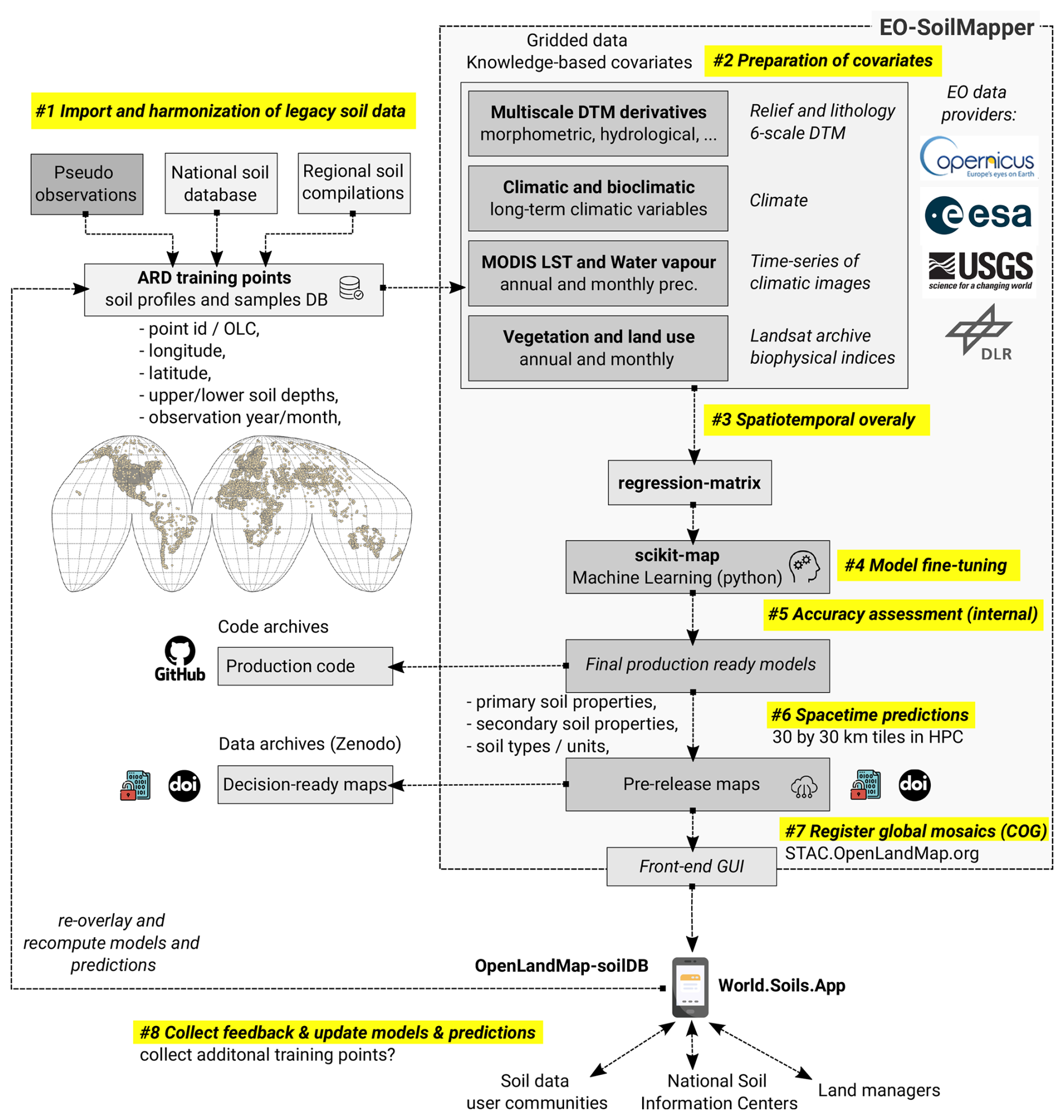
Figure 1 The general processing diagram of EO-SoilMapper with eight (8) key steps. This is a circlular and modular system with four main components developed independently: (1) standardized soil samples, (2) covariate layers, (3) the computing engine, and (4) back-end/front-end infrastructure for serving seamless data. ARD = Analysis-Ready Data, OLC = Open Location Code, DOI = Digital Object Identifier, DLR = The German Aerospace Center. Automation of modeling, model fine-tuning and prediction in this framework is important as it allows for updating the predictions as more training data is added.

Spatio-temporal Machine Learning (ML) implies (Hackländer et al., 2024; Tian et al., 2025b):

1. Spatio-temporal overlay: observations & measurements (O&M, such as observations of soil types, diagnostic horizons, laboratory measurements of soil pH, soil carbon content) are overlaid with covariate layers by matching both the geographic location and the start/end time period. In this paper, we only match O&Ms by year of sampling/field-work with covariate layers, although some soil properties, such as soil moisture, would also require refined temporal identification.

2. Strictly defined time-period of interest: covariate layers need to match the distribution of O&M's in the time domain, i.e., there needs to be enough training points spread across the period of interest (in this case 2000–2022+).

3. Spatio-temporal cross-validation: for accuracy assessment, we report both spatial blocking cross-validation and leave-one-year-out (LOYO) cross-validation to prevent producing over-optimistic validation results for densely sampled/clustered points, due to e.g. strong spatial auto-correlation.

4. Predictions in spacetime using spacetime blocks: predictions are strictly spatio-temporal, i.e., they are connected with certain begin/end time periods. We refer to the spacetime prediction reference as “spacetime blocks”.

2.2 Domain of interest: global land mask

We generate predictions for the global land mask at 30 m resolution within the 2000–2022+ period (with years 2023 and 2024 under production). To derive a consistent land mask, we used GDTM30 (global DTM at 30 m) (Ho et al., 2025) and time-series of land cover maps 2000–2022 (Zhang et al., 2021). We derived a long-term land mask based on a land-conservative assessment of the ocean mask for 2000–2022+, so that some pixels are potentially covered with water in more recent years.

We mask out the world's deserts and permanent ice to avoid predicting values or soil types for areas that are marginally soil (e.g. the Sahara desert) or are completely hidden. We recommend instead using standard values for shifting sand areas as follows:

• 0 value for soil carbon content/density, total N, P, and K;

• 100 % for sand content;

• 0 % for clay/silt content;

• 1.6 t m⁻³ for bulk density;

Producing global maps at 30 m requires a serious High Performance Computing infrastructure, beyond standard desktop computers. The 30 m resolution maps are about 70 times larger in size than 250 m resolution maps. The land mask at 30 m resolution in the EPSG:4326 projection system (WGS84) contains about 210 billion pixels, while without deserts and permanent ice, about 190 billion pixels. Predictions of 1 soil variable for 5-year periods for 3 standard depths with lower and upper prediction intervals account for about 9 trillion pixels; as size on disk, this results in about 5–10 TB of data (after compression). Because we also provide predictions for blocks of years, our outputs are even a few hundred times larger in size than the long-term 250 m products (Poggio et al., 2021).

2.3 Target soil variables of interest

As target variables of interest for dynamic soil mapping, we consider the list suggested by Chen et al. (2022), which is based on bibliometric analysis, and the variables listed in National Academies of Sciences, Engineering, and Medicine (2021). As Tier 1 variables of interest, we especially focus on soil organic carbon (SOC) content (g kg⁻¹), soil organic carbon density (SOCd, kg m⁻³), soil pH in H₂O, texture fractions (sand, silt, and clay) based on USDA system, bulk density (t m⁻³), and soil types. We use USDA and/or ISO variables and laboratory standards as much as possible, as these are documented in the highest detail and are often used in international projects; for example, we use Dry Combustion for SOC and USDA soil taxonomy for soil types, which is fully open access documentation available to everyone.

Soil organic carbon density (SOCd in kg m⁻³) can be estimated at the site level and is the central and most important variable of interest for global soil mapping. The SOCd can be used to derive the organic carbon stock in t ha⁻¹ (Hengl and MacMillan, 2019):

$$\begin{array}{}\text{(1)}& \begin{array}{rl}\mathrm{SOCd}\left[\mathrm{kg}{\mathrm{m}}^{-\mathrm{3}}\right]& ={\displaystyle \frac{\mathrm{SOC}\left[\mathit{\%}\right]}{\mathrm{100}}}\cdot \mathrm{BD}\left[\mathrm{kg}{\mathrm{m}}^{-\mathrm{3}}\right]\\ & \cdot \left(\mathrm{1}-{\displaystyle \frac{\mathrm{CF}\left[\mathit{\%}\right]}{\mathrm{100}}}\right)={\displaystyle \frac{\mathrm{SOCs}\left[\mathrm{kg}{\mathrm{m}}^{-\mathrm{2}}\right]}{\mathrm{HT}\left[\mathrm{m}\right]}}\end{array}\end{array}$$

where BD is the bulk density of fine earth, CF is the volumetric percent of coarse fragments, HT is the thickness of the horizon layer, and SOCs is the organic carbon stock of the soil for the specific depth interval. Correction for gravel content is necessary because only material less than 2 mm is analyzed for SOC concentration. In principle, SOCd (kg m⁻³) is strongly correlated with the SOC content (g kg⁻¹). However, depending on soil mineralogy and coarse fragment content, SOCd can differ from the SOC content. SOCd can be estimated per depth interval, then aggregated to produce SOC stocks. Note also that the values of the SOCs in kg m⁻² can also be expressed in t ha⁻¹, in which case a simple conversion formula can be applied:

$$\begin{array}{}\text{(2)}& \mathrm{1}\cdot \mathrm{kg}{\mathrm{m}}^{-\mathrm{2}}=\mathrm{10}\cdot \mathrm{t}{\mathrm{ha}}^{-\mathrm{1}}\end{array}$$

Total SOC in tonnes for an area of interest can be derived by multiplying SOCs (stocks) by total area e.g.:

$$\begin{array}{}\text{(3)}& \mathrm{SOCs}\cdot \mathrm{A}=\mathrm{120}\mathrm{t}{\mathrm{ha}}^{-\mathrm{1}}\cdot \mathrm{1}{\mathrm{km}}^{-\mathrm{2}}=\mathrm{120}\cdot \mathrm{100}=\mathrm{12}\mathrm{000}\mathrm{t}\end{array}$$

For example, a 0–10 cm soil layer with 0.82 % of SOC and bulk density of 1340 kg m⁻³ and 6 % coarse fragments, has a SOCd of 10.3 kg m⁻³, which corresponds to SOCs of 1.03 kg m⁻² (or 10.3 t ha⁻¹). An organic soil with 47.2 % of SOC and bulk density of 179 kg m⁻³ and 5 % coarse fragments in 0–30 cm, has a SOCd of 80.3 kg m⁻³, which corresponds to SOCs of 24 kg m⁻² (240 t ha⁻¹). A standard agricultural soil layer 0–30 cm with 1.5 % SOC and a bulk density of 1250 kg m⁻³ corresponds to SOCd of 18.75 kg m⁻³ i.e. a SOC stock of about 56 t ha⁻¹ (for 0–30 cm). Unfortunately, some authors use the metric t ha⁻¹, without indicating referent depth interval (e.g. 0–20, 0–30, 0–100, 0–200 cm) which can lead to confusion (the SOCs of 0–100 cm layer can often be 10 %–25 % higher than for 0–30 cm).

It is important to note that, to determine stocks using global maps, one first needs to reproject the SOCd predictions (kg m⁻³) onto some equal-area projection such as the Interrupted Goode Homolosine (IGH; EPSG:54052) (Steinwand, 1994). Next, multiply the SOCd in kg m⁻³ by the total area to obtain a total number of tons of SOC for the whole land mask. Another option is to determine the size of each pixel in WGS84 lon-lat projection system, although this can get computational. In this paper, we consistently visualize all the maps and determine all areas using the IGH projection.

2.4 Preparation of training points

As training points for global soil mapping, we use a compilation of harmonized and quality-controlled soil O&M's listed at https://soildb.OpenLandMap.org/ (last access: 6 June 2025), which took several years to organize, import, standardize and harmonize. The data sources for the training data included:

• Original national or regional monitoring networks with probability sampling, quality-controlled and maintained by federal/national agencies (L1);

• Original national or regional 1-time surveys with probability sampling, quality-controlled and fully documented (L2);

• Original regional or local soil sampling projects based on free-sampling (i.e. opportunistic sampling), but quality-controlled, and fully documented (L3);

• Compiled national or regional soil legacy O&M's data sets, quality-controlled and maintained; usually documented in a peer-review publication (L4);

• Compiled international, national or regional soil legacy O&M's data sets, quality-controlled and fully documented, but with significant missing information about laboratory methods (L5);

• Compiled international, national or regional soil legacy O&M's data sets, usually not quality-controlled, based on unknown methods, including based on citizen-science data (L6);

• Other soil legacy O&M's data sets without a peer-review publication, with significant missing information about laboratory methods (L7);

We have put the greatest effort into importing and binding L1–L3 data sets such as the National Cooperative Soil Survey Characterization Database (http://ncsslabdatamart.sc.egov.usda.gov/, last access: 6 June 2025) and the United States National Soil Information System, LUCAS soil (Orgiazzi et al., 2018), Brazilian PronaSolos (Polidoro et al., 2021), CSIRO's National Soil Site Database (CSIRO, 2024), Agriculture and Agri-Food Canada National Pedon Database (Geng et al., 2010), and the Mexican soil samples national inventory (Paz-Pellat and Velázquez-Rodríguez, 2018). These represent more than 80 % of the training points used and were essential to produce global predictions. The L1–L3 points are also the largest in volume, especially the NCSS Soil Characterization Database for the United States and a combination of LUCAS soil and national data sets for Europe.

From the 10 world's largest countries, the largest gaps in training data are because only very limited training data is available for 2000–2022 for India, the Russian Federation, China, and Kazakhstan. Although national data sets are available for Russia and China (Shangguan et al., 2013), these do not cover the 2000–2022 period and are relatively sparse. Similarly, the Canadian CUFS data set (Shaw et al., 2018) is a great open resource of soil laboratory data; however, it does not overlap in time with the 2000–2022+ period and, therefore, was not used for modeling.

From the L4 data set, we should especially emphasize the following four (each covering larger region/continent): Africa Soil Profile Database (Leenaars et al., 2014), Latin America and Caribbean Soil Information System (SISLAC) database (Díaz-Guadarrama et al., 2024), Northern circumpolar permafrost soil profiles (Hugelius et al., 2013a), and the Mangroves soil data base (Maxwell et al., 2023). We also used several global or near-global databases produced as compilations from old reports and scientific papers (L5), for example: ISRIC's WoSIS (Batjes et al., 2024), Fine Root Ecology Database (FRED) (Iversen et al., 2017), Soil Health DB (Jian et al., 2020), and the International Soil Carbon Network Database (Harden et al., 2018). Many of these are actually compilations of the above-listed national or regional databases and, as such, do not necessarily need to be imported, as this could lead to many duplicates (these would hence be a compilation of compilations). Some, however, contain additional smaller data sets contributed by smaller organizations or individuals. Thus, it was important to import and check all available point data sets to avoid missing out.

From citizen science data (L6) the significant data set is the LandPKS app (Quandt et al., 2018) observations (165 000 observations with coordinates on December 2024), which is currently the biggest L6-type soil data set for global soil mapping. Beyond citizen science data, we also used a significant number of pseudo-observations (documented in the next sections) to help also represent areas with extreme climate/landscape conditions, e.g. shifting sands/deserts, mountain peaks, and bare rock areas. Pseudo-observations were added primarily to represent and integrate soil knowledge into ML.

We provide all import and harmonization steps in https://soildb.OpenLandMap.org/ and explain how to access the analysis-ready compiled and harmonized soil samples. Some training soil points are proprietary as we have signed a data sharing agreement that limits us to share them publicly, but we always provide preparation steps and a description of the data so that eventually users can detect any potential standardization/harmonization issues.

For mapping soil types (USDA subgroups), we used a compilation of points provided by the USDA (about 320 000 locations with soil classification) and extended it with harmonized soil profiles from various other projects, especially WoSIS points and national soil profile data sets. To reduce global gaps, we put particular effort into translating some compatible national soil classification systems, e.g., the Brazilian soil classification system and the Canadian soil classification systems. Usually, we translate the input Canadian or Brazilian classes to the 2 to 3 most probable soil types using the recommended translation tables (Krasilnikov et al., 2009); translating to multiple classes is more realistic, but results in many duplicate points. This inherent classification uncertainty is further propagated in the models. However, to avoid any issues with poor translation, only the original high-quality USDA classes (un-harmonized) are used for validation (as hold-out samples).

In principle, only USDA soil points with soil types are fully harmonized and can be considered analysis-ready, while other data sets required careful checks and preparation, so they could also be included in the analysis. To speed up the cleaning up of points for soil type mapping, we used the following three strategies:

• We use fuzzy search strategies to avoid missing out points with possible types or missing “s” at the end of the soil type. For example, a text containing “typic haplaquoll, fine loamy mixed mesic” will be matched with the targeted soil type “typic haplaquolls”. Fuzzy matching has been implemented using the agrep function in R with max.distance=0.02, ignore.case=TRUE; this has been shown to perform the best in removing only incompatible classes.

• We search for soil types in multiple columns in the soil profile databases. For example, in the case of the Australian CSIRO NatSoil database, some USDA soil classification is only available in comments.

• We record all translations and soil types cleaning in one large Google Sheet so that all harmonization/translation steps can be back-tracked (see https://doi.org/10.5281/zenodo.4748499, Hengl and Gupta, 2025).

The import, translation and binding of soil-type training points are also fully documented in https://soildb.OpenLandMap.org/. In the end, these efforts provided a total of 332 thousand training points with soil type (USDA soil taxonomy subgroup), which yielded slightly more spatial locations than we prepared for soil property mapping. Unfortunately, most of the points (> 80 %) with USDA soil taxonomy are located in the USA and, as such, the North American continent is overrepresented in our models (see further Fig. 6b).

To quantify potential extrapolation problems due to spatial clustering and geographical gaps in point data, we run the Isolation Forest (Liu et al., 2008) on the training points and the selected most important covariates to produce an extrapolation risk probability map. This was only used to illustrate the effects of over-representation of training points and to suggest to next generation projects where to place more samples in the future to help improve these predictions.

2.5 Standardization and harmonization

Before spatial analysis, it is important to standardize (convert to the same measurement units, the same physical standards) and harmonize (bring to the same laboratory reference methods) soil laboratory data to avoid potential bias in predictions and could also have serious consequences on decision making. From all the variables analyzed in soil science, the organic carbon and texture fractions of the soil must be carefully treated because different countries use contrasting laboratory methods and standards, and the difference in values can often be considerable (> 5 % in relative terms). For example, soil organic carbon has historically been analyzed using a variety of laboratory methods, including (Chatterjee et al., 2009; Shamrikova et al., 2022):

• Walkley Black method (WB);

• Tyurin method;

• Dry Combustion method (DC);

• Loss on Ignition (LOI);

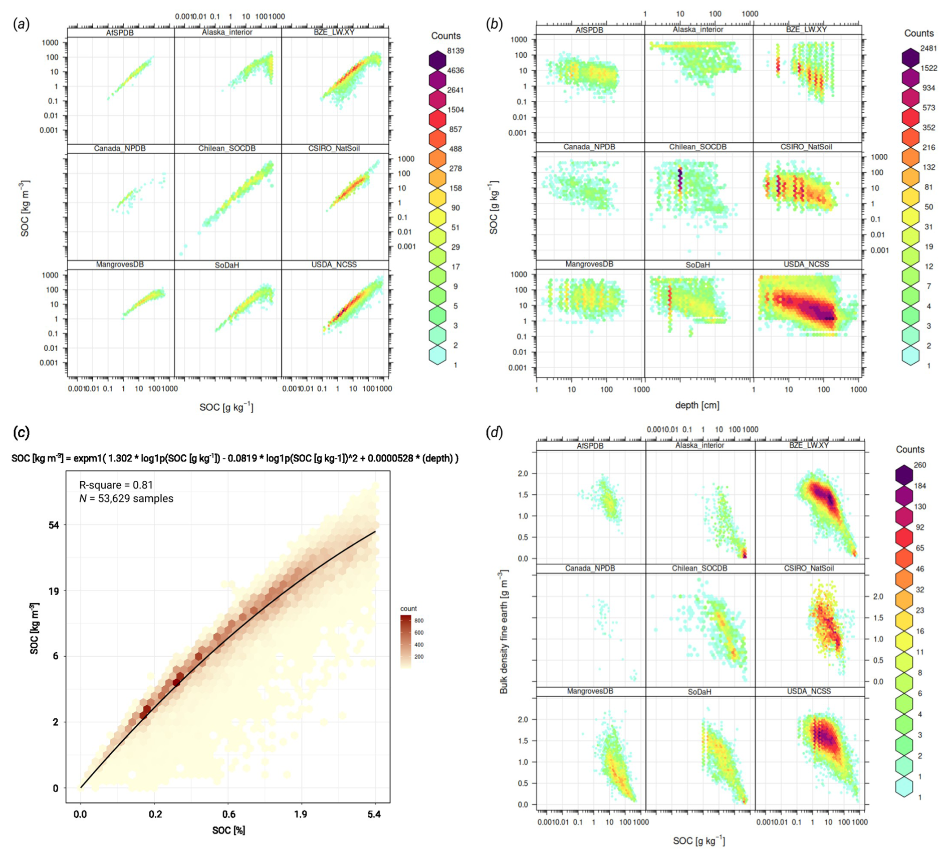
Figure 2 Comparison of imported soil laboratory data sets in terms of relationship between soil carbon density, carbon content, sampling depth, bulk density and others: (a) relationship between SOC content [g kg⁻¹] and SOC density (SOCd) [kg m⁻³] is often close to linear, although this relationship is significantly more diffuse for organic soils; (b) soil carbon – depth plots usually indicate negative log-log relationship; (c) a global pedo-transfer function fitted using the highest quality laboratory data to gap-fill low SOC density [kg m⁻³] values from SOC [g kg⁻¹] values; and (d) SOC [g kg⁻¹] and bulk density of fine-earth are also highly correlated and follow a bimodal distribution with one peak for mineral, and one for organic soils. AfSPDB = Africa Soil Profile Database (Leenaars et al., 2014), Alaska interior soil database (Manies et al., 2020), BZE-LW = Bodemzusandserhebung/German Agricultural Soil Inventory (Poeplau et al., 2020), Canada NPDB = Agri-Food Canada National Pedon Database (Geng et al., 2010), Chilean SOCDB = Chilean Soil Organic Carbon Database (Pfeiffer et al., 2020), CSIRO NatSoil (CSIRO, 2024), Mangroves soil database (Maxwell et al., 2023), SoDaH = the SOils DAta Harmonization database (Wieder et al., 2021), and USDA NCSS = National Cooperative Soil Survey Characterization Database.

All four SOC determination methods can be considered compatible; however, values need to be corrected to a common standard, otherwise, this can lead to bias in total stocks. For example, the DC method, which is the current recommended standard for soil organic carbon (ISO 10694:1995), produced about 20 %–40 % higher values than the WB method for the same samples. Locally, various groups have developed harmonization functions by analyzing the same soil samples using multiple laboratory methods (Chatterjee et al., 2009). In recent decades, numerous harmonization studies have been published producing functions and coefficients for translating SOC to the target laboratory method; however, these are often based on local data and therefore may not be globally applicable. Additionally, inter-laboratory comparisons that analyze samples from the same pedons have shown significant differences (Safanelli et al., 2023). This implies that the variation in the values of SOC, pH, and other soil properties comes in large part from short-range variability and the interlaboratory component, and not only from the harmonization strategy. Therefore, we have decided to use a simple harmonization principle described in Shamrikova et al. (2022):

$$\begin{array}{}\text{(4)}& \text{WB}\times \mathrm{1.3}=\text{Tyurin}\times \mathrm{1.15}=\text{DC}(P=\mathrm{0.95})\end{array}$$

We have applied this harmonization to any SOC data set with the laboratory method explained in the metadata. Where metadata do not provide any information, we looked at the year of sampling and country of origin, and we estimated the laboratory method based on indications from the literature. For most of the laboratory data (> 90 %) we had enough metadata to correctly determine the laboratory method used.

For carbon concentration and density values from the United States Soil Characterization Database (NCSS SCD) (United States Department of Agriculture and National Cooperative Soil Survey, 2023), several steps were taken to harmonize the different methods of estimating carbon, bulk density, and rock fragments. As carbon concentration measurement methods in NCSS SCD have shifted from WB to DC approaches (Soil Survey Staff, 2022), several regressions were used to harmonize all organic carbon measurements with WB to then integrate them into the larger global dataset by converting to DC using a previously fitted conversion model. Previous internal regressions that relate the SCD DC measurements to WB (Wills et al., 2013, 2014) have resulted in a contrasting relationship with the broader literature, so we decided to normalize all NCSS SCD carbon concentration values to WB to allow more widely accepted conversion equations to equivalent DC equations to be implemented. For all samples with DC total carbon (TC) estimates, we first regressed all samples with a 1:1 pH less than 7.4 (to exclude carbonates) against the WB measurements (WB = TC × 1.046, R²=0.92, N=8671). This allowed all DC total carbon measurements with pH < 7.4 to be converted to WB units. Then, for additional samples with higher pH values that had DC SOC values, pre-adjusted for carbonates, we regressed those carbon values against WB again to convert them to a common unit (WB = DC × 1.037, R²=0.90, N=175).

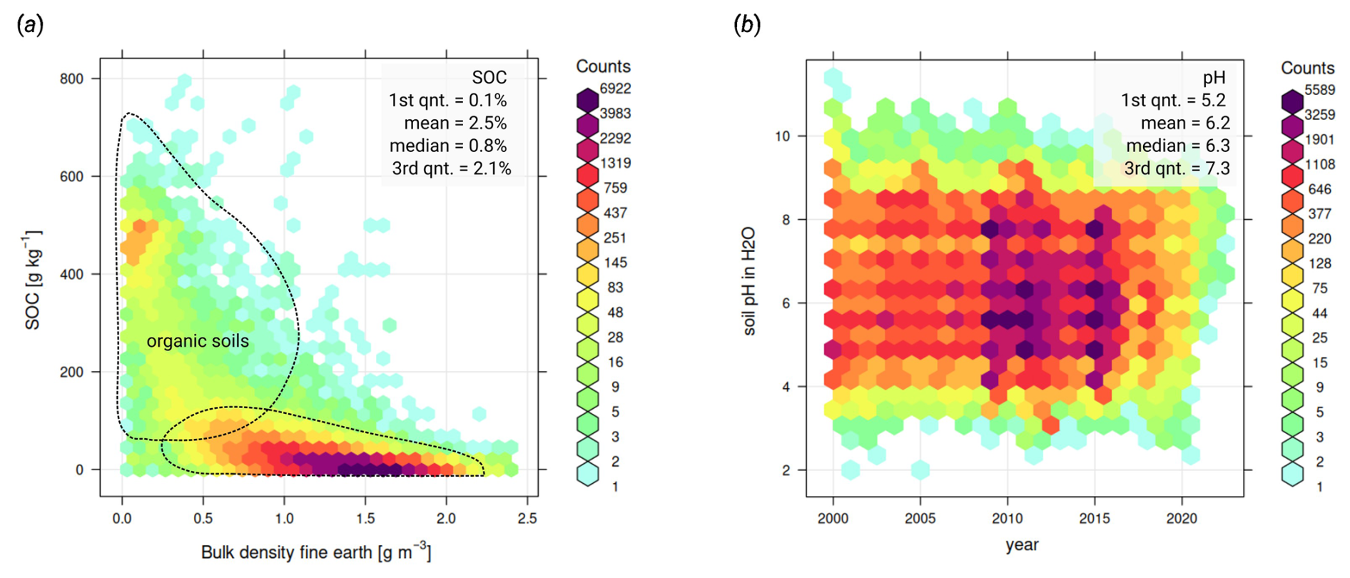
Figure 3 Density plots for the final global harmonized soil organic carbon and soil pH: (a) general relationship between soil organic carbon and bulk density with bimodal distribution of values (lines drawn by hand to illustrate overlap between organic and mineral soils), and (b) trend-plot showing, overall, no visible differences in soil pH distribution through time. Note that because SOC has a relatively right-skewed distribution, there is a significant difference in the mean value of SOC vs. the median value. Soil pH, on the other hand, is already log-transformed and hence the mean and median values more or less match.

In NCSS SCD, there are also more $\mathrm{1}/\mathrm{3}$ bar bulk density (BD.3) measurements available than oven dry bulk density (BDod); we therefore also regressed these two methods to maximize our sample size (BDod = BD.3 × 1.102, R² = 0.99, $N=\mathrm{90},\mathrm{230}$). We also tested regression models with intercept values for both carbon- and bulk-density models. Finally, to adjust the carbon densities for rock fragments, we analyzed the US NCSS National Soil Information System (NASIS) for all SCD samples. The SCD rock estimates only include fragments less than about 0.1016 m in diameter, so we opted to use the NASIS field total rock volume estimates, which include all rock sizes. A rock density of 2.65 t m⁻³ was assumed for all samples. Similar corrections were applied to other L1–L3 data sets used in this work.

2.6 Insertion of pseudo-observations and gap-filling of missing values

Most legacy soil data sets in the world were not generated using probability sampling and/or strict experimental designs and, as such, are often not directly fit for spatial modeling (Hendriks et al., 2019). If we were to ignore that some areas are over-represented, the resulting models fitted using such data could propagate potential bias in terms of, e.g. over-representation of agricultural land (Tian et al., 2025b). That is why it is important to add covariate layers and additional points to assist machine learning models in producing predictions that also better match expert knowledge (Minasny et al., 2024).

Insertion of pseudo-observations is especially important for mapping chemical and physical soil properties, soil carbon stocks, as otherwise one could significantly over- or underestimate global stocks. Consider the following two examples: (1) the majority of soil surveys ignore taking samples from C horizons (parent material layer), semi-desert and shifting sand areas as it is obvious to surveyors that these contain no SOC; (2) mountainous areas, inaccessible areas such as swamps, jungles and similar are also often under-represented due to inaccessibility. The world's deserts (polar deserts, Sahara, and similar) cover almost 33 % the Earth's land surface: approximately 20 % of the Earth's land surface are hot deserts; polar deserts (Antarctica and Greenland) cover another 10 %. Very few soil surveys actually go to the middle of a desert or on top of a mountain to collect soil samples.

To avoid over-predicting SOC and under-predicting sand content for the world, we added pseudo-training points to help incorporate our soil knowledge in ML. To generate pseudo-points, we used primarily the GLANCE data set (Stanimirova et al., 2023a), which is an extensive, quality-controlled point dataset covering years 1984 to 2020 and which is based on very high-resolution satellite images (usually about 30 cm resolution). We specifically used the classes “Bare rock” (5) and “Shifting sand, deserts without any vegetation” (6) as these are also easy to validate, and we believe that the risk of inserting erroneous pseudo-observations is low.

In addition to GLANCE points, we also used the global point data set with all major mountain tops (http://www.peaklist.org/ultras.html, last access: 6 June 2025; about 1500 mountain tops), also to avoid generating extrapolation for the highest mountain chains, such as the Alps, the Himalayas, and similar. These areas are often under-sampled or not represented at all because they are extremely inaccessible. To avoid adding false 0 points for SOC, we double-checked the pseudo-observation points by overlaying them vs. the 30 m resolution land cover map of the world GLC_FCS30D (Zhang et al., 2021). We only used the GLANCE point and the mountain tops that were also classified as “190 Impervious surfaces”, “200 Bare areas”, and/or “220 Permanent ice and snow”. In the end, this gave us 4680 high-quality pseudo-observations that are either permanent deserts, bare rock, or snow. At all these points, we have inserted 0 values for soil organic carbon (content and density), and also 100 % sand content for all points classified as sand in the GLANCE data set.

Note that we insert pseudo-observations for modeling purposes to better represent feature space, especially towards the edges of the feature space; however, after the modeling, we do not produce predictions for shifting sand areas and permanent ice as previously explained. This is for the following reasons: although we could have computed predictions for shifting sands and permanent ice, we believe that this would have increased production costs without adding significant value to the output maps. In addition, several covariates used for modeling are also often not accurate in such areas, potentially affecting the quality of the predictions. We, instead, advise users to gap-fill the maps using simple rules as indicated above or similar strategies (e.g. insert 0 SOC values and 100 % sand content for shifting sands).

In addition to inserting 0 values for obvious shifting sand/deserts and bare rock areas, we also gap-filled around 5 %–6 % soil carbon density points that only had SOC content but no bulk density. This was done by fitting a simple pedotransfer function (PTF) to estimate SOC [kg m⁻³] directly from SOC [g kg⁻¹] measurements, avoiding estimating the bulk density that would be used to calculate SOC [kg m⁻³]. We fit a bivariate quadratic function where the SOC density is a function of the SOC content and soil depth (shown in Fig. 2c), then use this function to fill in the missing values for the SOC density. We recommend using this PTF only for smaller values of SOC, e.g. < 0.5 % SOC, as the relationship for larger SOC values is of the order of magnitude more uncertain. In this work, we used this PTF to fill in gaps for the missing bulk density [kg m⁻³] only where the SOC content is < 0.4 % or < 4 ‰, as for this part of the range model it is significant with R²>0.96. The relationship between the density and content of SOC in soils with SOC > 1 % becomes proportionally more complex with a high uncertainty eventually for SOC > 10 %, and therefore we recommend using this PTF only for small values of SOC (< 0.4 %).

2.7 Preparation of covariate layers

To integrate land use changes, soil management, and climate effects, we used more than 160 TB of covariate data for modeling and prediction at 30 m resolution. The following four data sources are the largest in size and can be considered the most important:

• Landsat bimonthly and annual global composites described in Consoli et al. (2024) and derived products (Tian et al., 2025a; Isik et al., 2025) (30 m spatial resolution);

• 6-scale Digital Terrain Model relief parameters described in Ho et al. (2025) (multi-scale pyramid representation at 30, 60, 120, 240, 480, 960 m);

• CHELSA Climate time-series of climatic and bioclimatic variables v2.1 (Karger et al., 2017) (1 km spatial resolution);

• MODIS Land Surface Temperature MOD11A2 (https://doi.org/10.5281/zenodo.4527052, Hengl and Parente, 2021) and Water Vapor data sets MCD19A2 (https://doi.org/10.5281/zenodo.8226291, Parente et al., 2023) (1 km spatial resolution);

From the Landsat archive, we use the Blue, Green, Red, NIR, SWIR1, SWIR2 bands, and derivatives (biophysical indices) such as Normalized Difference Vegetation Index (NDVI), Normalized Difference Water Index (NDWI), Soil Adjusted Vegetation Index (SAVI), Bare Soil Index (BSI), Normalized Difference Tillage Index (NDTI), annual Bare Soil Frequency (BSF), Normalized Difference Snow Index (NDSI), Fraction of Absorbed Photosynthetically Active Radiation (FAPAR) and Gross Primary Productivity (Tian et al., 2025a; Isik et al., 2025). Although we originally considered using the bimonthly values of all variables, winter months in the northern hemisphere and heavily clouded areas, like rain forests, have been shown to carry a significant amount of artifacts, which can propagate to predictions and lead to more serious artifacts. To avoid such issues, we decided to only use the lower (25 % probability) annual quantile in the original bands instead of using bimonthly values or other quantiles. The decision to use the lower quantile comes from the fact that several artifacts originates from failing cloud mask, leading higher values in the raw bands, that are not impacting the lower quantiles. To keep a single consistent model, the usage of the lower quantile is applied at global scale, and not only in the areas with artifacts. However, it is possible that the prediction accuracy of soil properties could be further increased with further improvements in the Landsat composites.

From the DTM variables, we use 6-scale DTM global parameters derived at pixel resolutions of 30 m and of 60, 120, 240, 480 and 960 m, which were later resampled to 30 m using cubic splines. The DTM variables include terrain height, slope in degrees, multidirectional hillshade, topographic wetness index, negative/positive openness, LS factor, minimum, maximum, profile, tangential and ring curvature. This type of multi-scale nested terrain derivation is known as “Mixed scaled Gaussian Pyramid” (Behrens et al., 2018), designated to capture spatial dependencies and interactions of the landscape and soil at various scales. Relationships between different soil properties and terrain change at different spatial resolutions are often in a non-linear way. Hence, we prepare standard DTM variables from fine to coarse resolution (microscale, mesoscale, and macroscale) to allow ML to select an optimal set of terrain representation based on the training data.

Beyond the above listed-layers, we also use: peatland extent ensemble estimate (https://doi.org/10.5281/zenodo.13951438, Hengl, 2025), bare rock extent based on the Local Climate zones map (Demuzere et al., 2022), forest and wetlands cover based on ESA CCI (https://doi.org/10.5281/zenodo.13951438, Hengl, 2025), crop cover based on GLAD time-series 30 m (Potapov et al., 2022), World Karst Aquifer Map (WHYMAP WOKAM) (Chen et al., 2017), sediment types based on GUM v1.0 (Börker et al., 2018), bare soil fractions (mean and maximum) and photosynthetically active vegetation fractions based on GVFCP v3.1 (https://doi.org/10.5281/zenodo.11961219, Hengl, 2024), Global WaterPack annual water extent probability (250 m) (Klein et al., 2017), snow probability P90 long-term MODIS-based (https://doi.org/10.5281/zenodo.5774953, Hengl, 2021), soil salinity grade (250 m) (Ivushkin et al., 2019), Global Soil Bioclimatic variables (Lembrechts et al., 2022), geometric temperature, landform class based on the USGS EcoTapestry, and MERIT Hydro upstream area (Yamazaki et al., 2019). Because the Global Soil Bioclimatic variables are also based on SoilGrids (sand, silt, clay predictions) and soil salinity grade is also based on soil property predictions, we use these layers only for soil type mapping and not soil property mapping, to avoid possible circularity in the models.

For quantitative soil properties, we also use soil depth (center of the sample horizon) as a covariate. This means that all such models are 3D+T, i.e. we fit one model per property that can be used to predict values for any year and for any depth. As further detailed in the following, predictions are then averages over spatio-temporal blocks of five years (e.g. 2000–2005) and variable depths interval (0–30, 30–60 and 60–100 cm). However, we did not use the month of field observation of the year of sampling as a covariate because this has been shown to lead to artifacts. In addition, because majority of covariates are time-series of annual/bimonthly images, time is already deeply embedded in the covariates; hence, we do not find it necessary to also include it as a continuous variable.

In summary, we used a total of 363 covariate layers for mapping soil properties and soil types, either as time series of bimonthly/annual images from 2000–2022+, long-term estimates of climate, or assumed static variables (DTM parameters, lithology types, and similar). For soil type mapping, we used a much smaller number (229) of covariate layers because we excluded all time-varying layers, and hence only long-term estimates of climate, vegetation and similar are used. Not all layers were used in the final prediction as the feature selection process would typically reduce the number of initial number of layers to 60–120, removing layers that marginally contributed to the final model.

2.8 Variables transformation for soil properties

To account for a highly skewed distribution of soil organic carbon, both content and density, these properties were transformed into a natural log (with offset = 1, ln (x+1)). Tian et al. (2025b) show that using log-transformation before modeling helps increase accuracy, especially accuracy of lower values (agricultural soils) i.e. helps decrease impact of a small portion of very high SOC values in the organic soil. Once the target variable is transformed to a close-to-normal distribution, visualization of data and derivation of standard linear regression metrics such as R², RMSE and similar are possible. This means that we automatically transform all log-normal variables and do all modeling in log-space. The final predictions are then back-transformed (exp (x)−1) in the original space in the last step. We report error metrics for log-normal variables in both original and transformed spaces.

Soil texture fractions are transformed using a modified version of the additive log-ratio (ALR) transform, which for the forward transformation reads:

$$\begin{array}{}\text{(5)}& \begin{array}{rl}{\text{Texture}}_{\mathrm{1}}& ={\log }_{\mathrm{2}}\left({\displaystyle \frac{\frac{\text{Sand}}{a}+\mathrm{1}}{\frac{\text{Clay}}{a}+\mathrm{1}}}\right),\\ {\text{Texture}}_{\mathrm{2}}& ={\log }_{\mathrm{2}}\left({\displaystyle \frac{\frac{\text{Silt}}{a}+\mathrm{1}}{\frac{\text{Clay}}{a}+\mathrm{1}}}\right).\end{array}\end{array}$$

where a is a normalization factor corresponding to the summation value of the three fractions (e.g. 100 if they are represented in %). The new transformation removes the singularities that are present in the ALR transformation if one or more of the textures fractions is equal to zero. Furthermore, the usage of log ₂ and the normalization by a of each texture in the forward transformation guaranty that both variables in the transformed space are in the range −1 and 1. For the data collected in this work, the distributions of Texture₁ and Texture₂ are close to a uniform distribution and a normal distribution, respectively. These properties facilitate the modeling phase compared to having skewed, sparse distributions or numerically noisy values that were observed using standard ALR transform. The variables Texture₁ and Texture₂ are then modeled and predicted separately. This leads to no guaranty that after applying a straightforward back-transformation to the predictions, the texture fractions would sum up to a, nor that each of them is greater than or equal to 0. For these reasons, the back-transformation applied to the prediction is slightly modified to guaranty that these constraints are respected, and it reads:

$$\begin{array}{}\text{(6)}& {\displaystyle }{x}_{\mathrm{1}}& {\displaystyle }={\mathrm{2}}^{{\text{Texture}}_{\mathrm{1}}},x_{\mathrm{2}}={\mathrm{2}}^{{\text{Texture}}_{\mathrm{2}}},\text{(7)}& {\displaystyle }C& {\displaystyle }=max\left(\mathrm{0},{\displaystyle \frac{\mathrm{3}-x_{\mathrm{1}}-x_{\mathrm{2}}}{\mathrm{1}+x_{\mathrm{1}}+x_{\mathrm{2}}}}\right),\text{(8)}& {\displaystyle }S& {\displaystyle }=max\left(\mathrm{0},x_{\mathrm{1}}C+x_{\mathrm{1}}-\mathrm{1}\right),\text{(9)}& {\displaystyle }L& {\displaystyle }=max\left(\mathrm{0},x_{\mathrm{2}}C+x_{\mathrm{2}}-\mathrm{1}\right),\text{(10)}& {\displaystyle }T& {\displaystyle }=S+L+C,\text{(11)}& {\displaystyle }\text{Sand}& {\displaystyle }={\displaystyle \frac{a}{T}}S,\text{Silt}={\displaystyle \frac{a}{T}}L,\text{Clay}={\displaystyle \frac{a}{T}}C.\end{array}$$

2.9 Model calibration and prediction of soil properties

For each property, the data set is first partitioned into three subsets: (1) calibration, (2) training, and (3) stratified test sets, with an approximate ratio of $\mathrm{1}:\mathrm{8}:\mathrm{1}$. The calibration set is used for feature selection and hyperparameter tuning, the training set for model development, and the hold-out test set for final evaluation. The hold-out test set is not used for any other purpose but for accuracy assessment. When the data set is large, to prevent the excessive data volume from skewing the process, we cap the calibration and test set sizes at 8000 and 6000 samples, respectively. For calibration and test sets, we use spatial subsetting with a standard density of points per 100 km by 100 km tile (for example, a maximum of 2 points per tile). This ensures that the overall density of points is standard and that there are no geographical groups (Roberts et al., 2017), similar to the approach used in Poggio et al. (2021). The data set partition scheme is represented in Fig. 4.

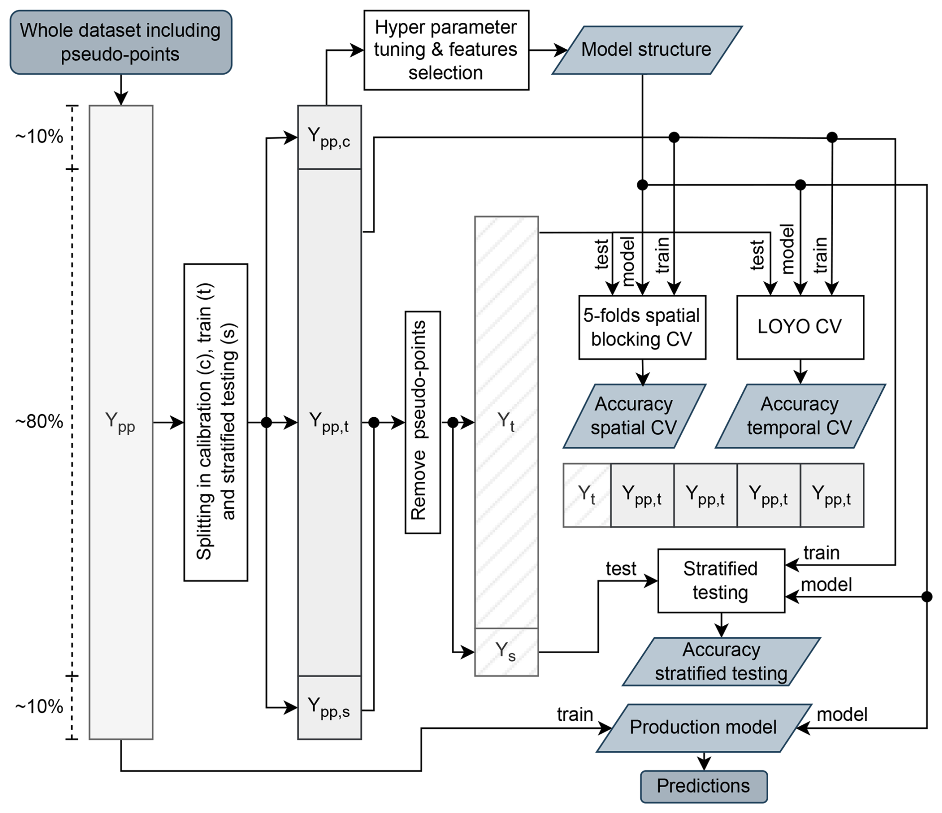
Figure 4 Schematic partition of the soil properties dataset. For each property, the whole dataset including pseudo-points (Y_pp) is divided in calibration (Y_pp,c), training (Y_pp,t), and stratified test (Y_pp,s) sets, with an approximate ratio of $\mathrm{1}:\mathrm{8}:\mathrm{1}$. The calibration dataset is used to perform hyper parameters tuning and features selection. The optimized model structures is trained with the Y_pp,t set under three different validation setups: stratified testing, 5-folds spatial blocking CV and leave-one-year-out (LOYO) CV. In all the testing phases of the validation, the pseudo-points were removed from the test sets, so using Y_s or splits of Y_t. The obtained results are used to derive all the reported accuracy metrics. The whole dataset is instead used to train the final model used for predictions.

For feature selection, we use Repeated Subsampling-Based Cumulative Feature Importance (RSCFI), a variant of Recursive Feature Elimination with Cross-Validation (RFECV) (Wadoux et al., 2020). RSCFI optimizes model performance while efficiently eliminating less relevant covariates, achieving results comparable to those of RFECV. Hyperparameter tuning is performed using HalvingGridSearchCV (Pedregosa et al., 2011), a resource-efficient approach that iteratively narrows down the best parameter combinations, optimizing the Lin’s Concordance Correlation Coefficient (CCC).

After calibration and accuracy assessment, the whole dataset was used to train the Tree-Based Quantile Regression Forest (TB-QRF) and the RF models. We used the compiled versions of these models to produce predictions at 30 m resolution. In addition, we used the non-compiled version of the models to retrieve the single-tree outputs to produce 120 m resolution maps that also include quantiles 0.16 and 0.84 for uncertainty estimation. The entire pipeline has been developed using open-source code and integrated into the scikit-map library (https://github.com/openlandmap/scikit-map, last access: 6 June 2025). The combination of QRRF and RSCFI helps reduce model complexity, without suffering from multicollinearity effects. We consider the QRRF and RSCFI combination, hence, to be over-fitting-proof and not impacted with the multicollinearity in covariates.

The predictions are run per 1° by 1° tiles (∼ 120 km by ∼ 120 km) using parallel computing over 10 CPU servers and by reading from 17 storage servers to the central storage data lake (SeaweedFS file service). The world land mask can be represented with about 18 500 120 km tiles. After predicting target variables per tile, global mosaics are built using GDAL to produce complete, consistent Cloud-Optimized GeoTIFFs, one global scale (whole land mask) file for each combination of variable, time-frame, depth-range, and mean or quantile. Prediction is the most costly part of the data production, with each soil property taking at least 3 d of HPC with about 1500 threads and 14 TB of RAM to produce space-time predictions of a single soil property. The final output mosaics contain variable type, reference method and measurement units, depth interval, and reference begin/end year in the file name (see https://github.com/openlandmap/soildb, last access: 6 June 2025, for more details).

2.10 Block predictions in spacetime

We produce in memory point predictions for the years 2000, 2005, 2010, 2015, 2020 and 2022, and soil depths 0, 30, 60, and 100 cm; these are then averaged in 2 by 2 spatio-temporal blocks that represent timeframes of 5 years with one year overlap (excluding the last timeframe) and variable depth ranges:

$$\begin{array}{}\text{(12)}& {\text{spb}}_{i,j}={\displaystyle \frac{P_{i,j}+P_{i+\mathrm{1},j}+P_{i,j+\mathrm{1}}+P_{i+\mathrm{1},j+\mathrm{1}}}{\mathrm{4}}},\end{array}$$

as also shown in Fig. 5.

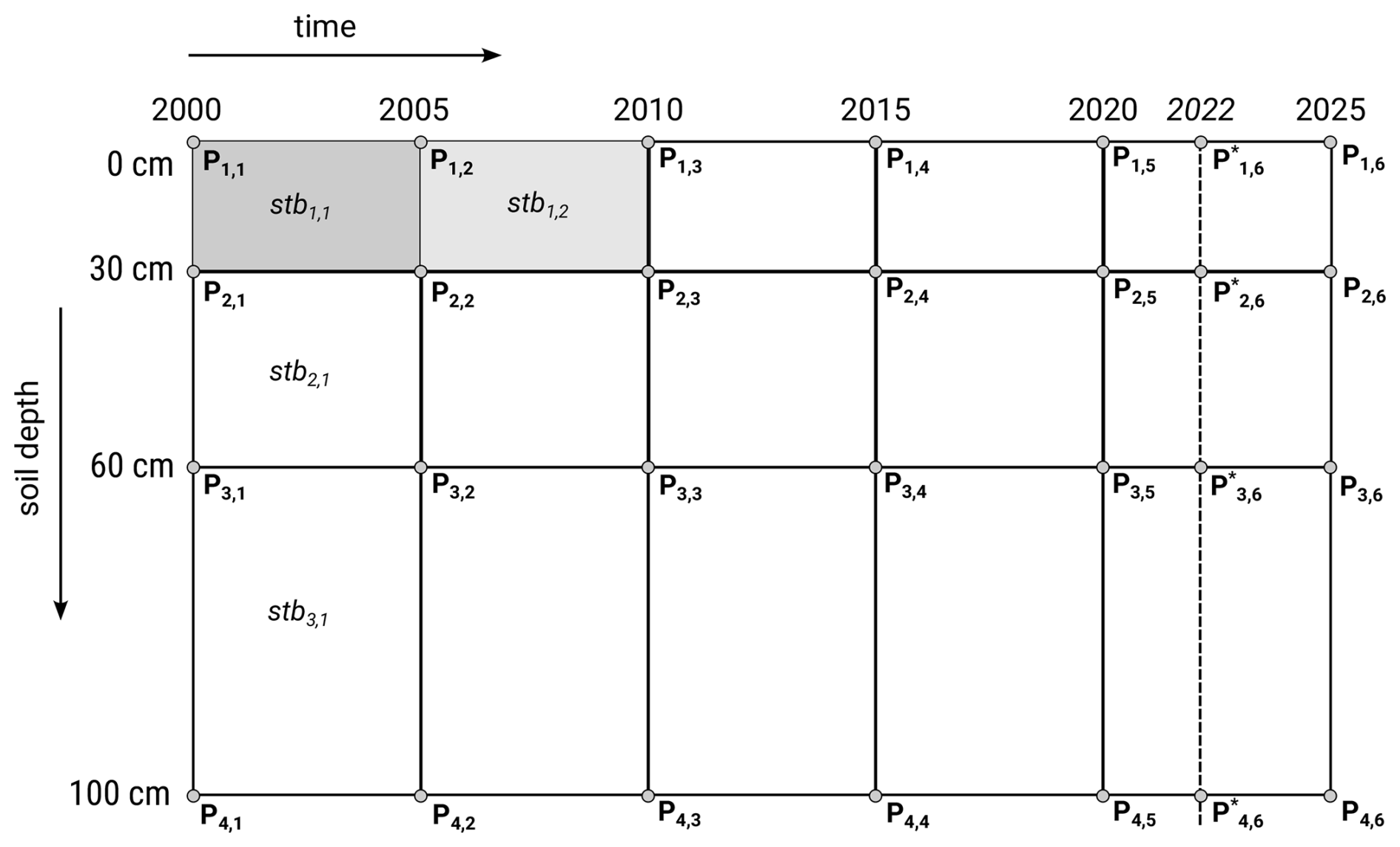
Figure 5 Spatio-temporal prediction blocks scheme: predictions are generated for four space-time points, then averaged to derive mean prediction and lower and upper prediction intervals. Note that at the time of analysis no ARD Landsat data was available for 2023–2025, hence for the last period the block support is < 5 years.

We decided to use block predictions as most of the users require predictions of soil properties per standard depth intervals. We also block-predictions in time primarily to reduce interannual variability, especially interannual oscillations coming from Landsat-derived indices. Note that while depth is a feature of the model, the prediction year is not. However, the prediction year was used to determine the specific layers to use in time-dependent features, so the models are fully temporally consistent.

2.11 Derivation of the per-pixel prediction uncertainty

To produce per-pixel uncertainty, we use the TB-QRF (Meinshausen, 2006), where the output of each single tree in the RF has been used to derive the prediction intervals:

$$\begin{array}{}\text{(13)}& \begin{array}{rcl}{\widehat{y_{\mathrm{1}}}}_{{\mathrm{stb}}_{\mathrm{1},\mathrm{1}}}& =& [P_{\mathrm{1},\mathrm{1}},P_{\mathrm{1},\mathrm{2}},P_{\mathrm{2},\mathrm{1}},P_{\mathrm{2},\mathrm{2}}]\\ {\widehat{y_{\mathrm{2}}}}_{{\mathrm{stb}}_{\mathrm{1},\mathrm{1}}}& =& [P_{\mathrm{1},\mathrm{1}},P_{\mathrm{1},\mathrm{2}},P_{\mathrm{2},\mathrm{1}},P_{\mathrm{2},\mathrm{2}}]\\ {\widehat{y_{\mathrm{3}}}}_{{\mathrm{stb}}_{\mathrm{1},\mathrm{1}}}& =& [P_{\mathrm{1},\mathrm{1}},P_{\mathrm{1},\mathrm{2}},P_{\mathrm{2},\mathrm{1}},P_{\mathrm{2},\mathrm{2}}]\\ \mathrm{\cdots }& & \\ {\widehat{y_N}}_{{\mathrm{stb}}_{\mathrm{1},\mathrm{1}}}& =& [P_{\mathrm{1},\mathrm{1}},P_{\mathrm{1},\mathrm{2}},P_{\mathrm{2},\mathrm{1}},P_{\mathrm{2},\mathrm{2}}]\end{array}\end{array}$$

where ${\widehat{y_{\mathrm{1}}}}_{{\mathrm{stb}}_{\mathrm{1},\mathrm{1}}}$ is the mean prediction from the individual tree (out of a total of N trees). These are then used to derive the lower and upper 68 % probability quantiles:

$$\begin{array}{}\text{(14)}& {\displaystyle }{\widehat{y}}_{\mathrm{lower}}& {\displaystyle }=Q_{\mathrm{0.16}}\left(\left\{{\widehat{y_{\mathrm{1}}}}_{{\mathrm{stb}}_{\mathrm{1},\mathrm{1}}},{\widehat{y_{\mathrm{2}}}}_{{\mathrm{stb}}_{\mathrm{1},\mathrm{1}}},\mathrm{\cdots },{\widehat{y_N}}_{{\mathrm{stb}}_{\mathrm{1},\mathrm{1}}}\right\}\right),\text{(15)}& {\displaystyle }{\widehat{y}}_{\mathrm{upper}}& {\displaystyle }=Q_{\mathrm{0.84}}\left(\left\{{\widehat{y_{\mathrm{1}}}}_{{\mathrm{stb}}_{\mathrm{1},\mathrm{1}}},{\widehat{y_{\mathrm{2}}}}_{{\mathrm{stb}}_{\mathrm{1},\mathrm{1}}},\mathrm{\cdots },{\widehat{y_N}}_{{\mathrm{stb}}_{\mathrm{1},\mathrm{1}}}\right\}\right).\end{array}$$

Note that compared to other QRF the distribution is obtained from a list of tree outputs and not from the single leafs. We decided to predict the quantiles 0.159 and 0.842 to lead to a 68 % interquartile range (IQR) and assuming a Gaussian distribution, 68 % interval corresponds to the ±1 standard deviation. To derive 1 standard deviation prediction error from the lower and upper intervals, users should calculate the range and then divide by 2.

In addition, compared to 90 % or 95 % IQRs, this allows us to have a smaller number of trees (e.g. 64) in the RF without leading to artifacts in case of noisy trees or covariates that are generally in the extremes of the distribution, and therefore speed-up computing. For variables with more complex distributions, for example, log-normal, gamma, or multi-modal distributions, dividing the upper minus lower range by 2 should be used with caution, as also the prediction distributions per pixel are often skewed, and hence the true errors might not match the approximated 1 std. It is also possible to save all N trees as independent predictions, and hence the users could then derive any arbitrary quantile or do per-pixel statistical tests.

To derive both predictions and prediction uncertainty on a global scale, we used a hybrid Python/C++ implementation of TB-QRF and RF Python/C++ where the models are fitted using the scikit-learn library in Python, then translated to C++ source code and compiled using tl2cgen. Spatio-temporal overlay and predictions were also performed using C++ interfaced with Python within the scikit-map library. Finally, although TB-QRF is a fairly robust method and is applied to all regression problems, it can sometimes over- or under-estimate actual prediction errors, and therefore we also test the accuracy of the prediction intervals using the procedure described in Tian et al. (2025b).

2.12 Model calibration and prediction for soil types

For modeling and mapping soil types, we also use the RSCFI framework, but with the difference that we develop two models: RF and LightGBM (Ke et al., 2017); the final predictions are then generated as an ensemble model by averaging the two. The approach is based on fitting models to features that are potentially valuable and selecting them based on the mean decrease in impurity. To enhance robustness, the model was trained 50 times, each time using different bootstrap-sampled subsets (80 %) of the calibration data set, selected by spatial blocking (100 by 100 km blocks). Features below the mean importance threshold were discarded in each iteration. To optimize computational burden, we selected 100 features that were consistently repeated in at least 25 model runs in both models. The final selected features were applied to the calibration and validation data sets before hyperparameter tuning.

2.13 Cross-validation and quality control

We decided to run the evaluation of soil properties models in three different modalities: (i) on a test set derived from stratified sampling based on Köppen–Geiger climate classification from CHELSA V.2.1 (Karger et al., 2017), (ii) with a 5-fold spatial blocking CV with 100 km by 100 km tiles, and temporal CV using the leave-one-year-out (LOYO) approach (Fig. 4). We consider the results of the accuracy assessment using the test set to give an overoptimistic estimate of the mapping accuracy and the results of temporal and spatial CV to give an over-pessimistic estimate: we expect that the actual accuracy is between the two numbers.

For each model, we report RMSE, mean error (bias), R-squared (R²), Lin’s concordance correlation coefficient (CCC), defined as:

$$\begin{array}{}\text{(16)}& \begin{array}{rl}& \mathrm{RMSE}=\sqrt{{\displaystyle \frac{\mathrm{1}}{n}}\sum _{i=\mathrm{1}}^n(y_i-{\widehat{y}}_i{)}^{\mathrm{2}}},\\ & \mathrm{bias}={\displaystyle \frac{\mathrm{1}}{n}}\sum _{i=\mathrm{1}}^n(y_i-{\widehat{y}}_i),\\ & R^{\mathrm{2}}=\mathrm{1}-{\displaystyle \frac{{\sum }_{i=\mathrm{1}}^n(y_i-{\widehat{y}}_i{)}^{\mathrm{2}}}{{\sum }_{i=\mathrm{1}}^n(y_i-\overline{y}{)}^{\mathrm{2}}}},\\ & \mathrm{CCC}={\displaystyle \frac{\mathrm{2}r{s}_y{s}_{\widehat{y}}}{(\overline{y}-\overline{\widehat{y}}{)}^{\mathrm{2}}+s_y^{\mathrm{2}}+s_{\widehat{y}}^{\mathrm{2}}}},\end{array}\end{array}$$

and the fraction of Tweedie deviance explained (D²) (Hastie et al., 2015; Pedregosa et al., 2011), calculated as:

$$\begin{array}{}\text{(17)}& \begin{array}{rl}& d(y_i,{\widehat{y}}_i)=\\ & \left\{\begin{array}{ll}(y_i-{\widehat{y}}_i{)}^{\mathrm{2}},& p=\mathrm{0}\text{(Normal)}\\ \mathrm{2}\left[y_i\log \left(\frac{y_i}{{\widehat{y}}_i}\right)-y_i+{\widehat{y}}_i\right],& p=\mathrm{1}\text{(Poisson)}\\ \mathrm{2}\left[\log \left(\frac{{\widehat{y}}_i}{y_i}\right)+\frac{y_i}{{\widehat{y}}_i}-\mathrm{1}\right],& p=\mathrm{2}\text{(Gamma)}\\ \mathrm{2}\left[\frac{y_i^{\mathrm{2}-p}}{(\mathrm{1}-p)(\mathrm{2}-p)}-\frac{y_i{\widehat{y}}_i^{\mathrm{1}-p}}{\mathrm{1}-p}+\frac{{\widehat{y}}_i^{\mathrm{2}-p}}{\mathrm{2}-p}\right],& \text{otherwise}\end{array}\right.\\ & D^{\mathrm{2}}=\mathrm{1}-{\displaystyle \frac{{\sum }_{i=\mathrm{1}}^{n}d(y_i,{\widehat{y}}_i)}{{\sum }_{i=\mathrm{1}}^{n}d(y_i,\overline{y})}},\end{array}\end{array}$$

where y_i is the observed value, ${\widehat{y}}_i$ is the predicted value, $\overline{y}$ is the mean value, n is the total number of samples, r is the Pearson correlation between y and $\widehat{y}$, $s_y^{\mathrm{2}}$ is the variance of the observed values, $s_{\widehat{y}}^{\mathrm{2}}$ is the variance of predicted values, and $\overline{\widehat{y}}$ is the mean of predicted values. Finally, to asses performance in quantifying uncertainty, we also report Prediction Interval Coverage Probability (PICP), computed as the ratio of actual values that reside inside a model's estimated confidence intervals for the corresponding predictions.

For cross-validation, we consistently make sure that training vs. validation data do not have the same coordinates, i.e. do not belong to the same sites. Using samples from the same profiles has been shown to lead to over-fitting as the model is able to cross-predict values; therefore, blocking values and enforcing an equal spread of points throughout the globe is important to avoid biased predictions (Roberts et al., 2017; Hackländer et al., 2024).

Note that, for log-normally distributed variables such as SOC, we report RMSE and CCC in log-space. Although RMSE in log-scale is abstract and difficult to interpret, however, for log-normal variables RMSE in original scale is often overly sensitive to high values (e.g. < 1 % very high values can double or triple RMSE), so that it becomes difficult if not impossible to compare performance of two models. Log-scale RMSE, on the other hand, allows comparing predictive performance of models where SOC training points come from either agricultural or forest soils. We further use log-scale RMSE to run simulations (using log-normal distribution) to try to detect numeric resolution and detectable changes in SOC.

2.14 Spatial dependence analysis for residuals

To evaluate the spatial structure of the prediction residuals, we computed empirical semivariograms of the absolute prediction errors. In an operational setting, this means that variograms are fitted per each of the six continents (Antarctica is excluded). Prediction errors were obtained through 10-fold cross-validation explained in the previous sections. The coordinates were reprojected to continent-specific azimuthal equidistant projections (Equi7) to assist in the distance calculation (Bauer-Marschallinger et al., 2014). For each continent, pairwise distances and squared differences in prediction errors were computed, and the empirical variogram was derived by binning these differences into 5 km distance intervals, up to a maximum lag of 125 km. A Locally Weighted Scatterplot Smoothing (LOWESS) smoothing line was fitted to the binned semi-variance estimates to visualize spatial trends. To support interpretation, we also fit spherical variogram models to data within a truncated spatial range of 125 km. GLanCE pseudo-observations were excluded from the analysis to avoid distortion of spatial dependencies.

2.15 Soil property change analysis against land cover change

To compare changes in soil properties for 2000 to 2022+ versus land cover change, we used a total of 12 500 unique spatial locations sampled following the strategy described in Hackländer et al. (2024). This is a point data set generated using the stratified random sampling approach and excluding areas covered by permanent water or ice (Brus, 2022). Each sampled point was overlaid with predicted maps of SOCd and pH for the periods 2000–2005 and 2020–2022, as well as the ESA CCI land cover maps for the years 2000 and 2020 (ESA, 2017). Based on this overlaid dataset, spatially matched changes in SOCd and pH were derived and linked to the corresponding land cover transitions for analysis and visualization. For each change class (e.g. broad-leave forest to pasture), we derive the mean SOCd and soil pH change value and the distribution of values. These values are then reported and sorted to see which land use change categories result in larger changes in soil properties, i.e. to detect which are the key drivers of change.

2.16 Extrapolation risk assessment

Extrapolation often leads to decreased performance in machine learning models, but it is an unavoidable aspect of large-scale spatial mapping. Several methods exist to identify predictions made in dissimilar feature spaces, including the Area of Applicability (AOA) (Meyer and Pebesma, 2021), Isolation Forest (Liu et al., 2008), and Homosoils (Nenkam et al., 2022). Given the extensive spatial scope and computational demands of this study, we selected the Isolation Forest algorithm due to its efficiency and suitability for non-normally distributed multivariate datasets (Liu et al., 2008). Isolation Forest detects regions of the feature space that differ from the training data by recursively partitioning the dataset and isolating individual samples. It works by constructing an ensemble of randomly generated trees and calculating an anomaly score based on the average path length required to isolate a sample. Samples located in low-density or unfamiliar regions of the feature space generally require fewer partitions, resulting in shorter path lengths and thus higher anomaly scores. We used the ensemble.IsolationForest implementation of scikit-learn (Pedregosa et al., 2011) to generate these scores. The average path length within the training data set serves as a baseline threshold to distinguish between in-sample and out-of-sample predictions (Liu et al., 2008). To effectively communicate the extrapolation risk to users, we normalize the anomaly scores on a scale 0–1, where higher values represent greater extrapolation risk for a given sample or pixel. The threshold separating the in-sample and out-of-sample regions was similarly rescaled to this normalized scale, ensuring consistency with the extrapolation risk probability maps delivered to end users.

3 Results

3.1 Harmonization of training data

After multiple rounds of import, binding and internal tests, we finally prepared about 216 000 soil samples with soil carbon density (kg m⁻³), 408 000 soil samples with soil carbon content (g kg⁻¹), 272 000 samples with soil pH in H₂O, 363 000 samples with clay, silt, and sand content (%), and 134 000 samples with bulk density oven dry (t m⁻³), which we consider to be analysis-ready. The additional samples from pseudo-observations from the PTF helped us increase the number of training points for mapping the SOC density from 227 000 to 305 820.

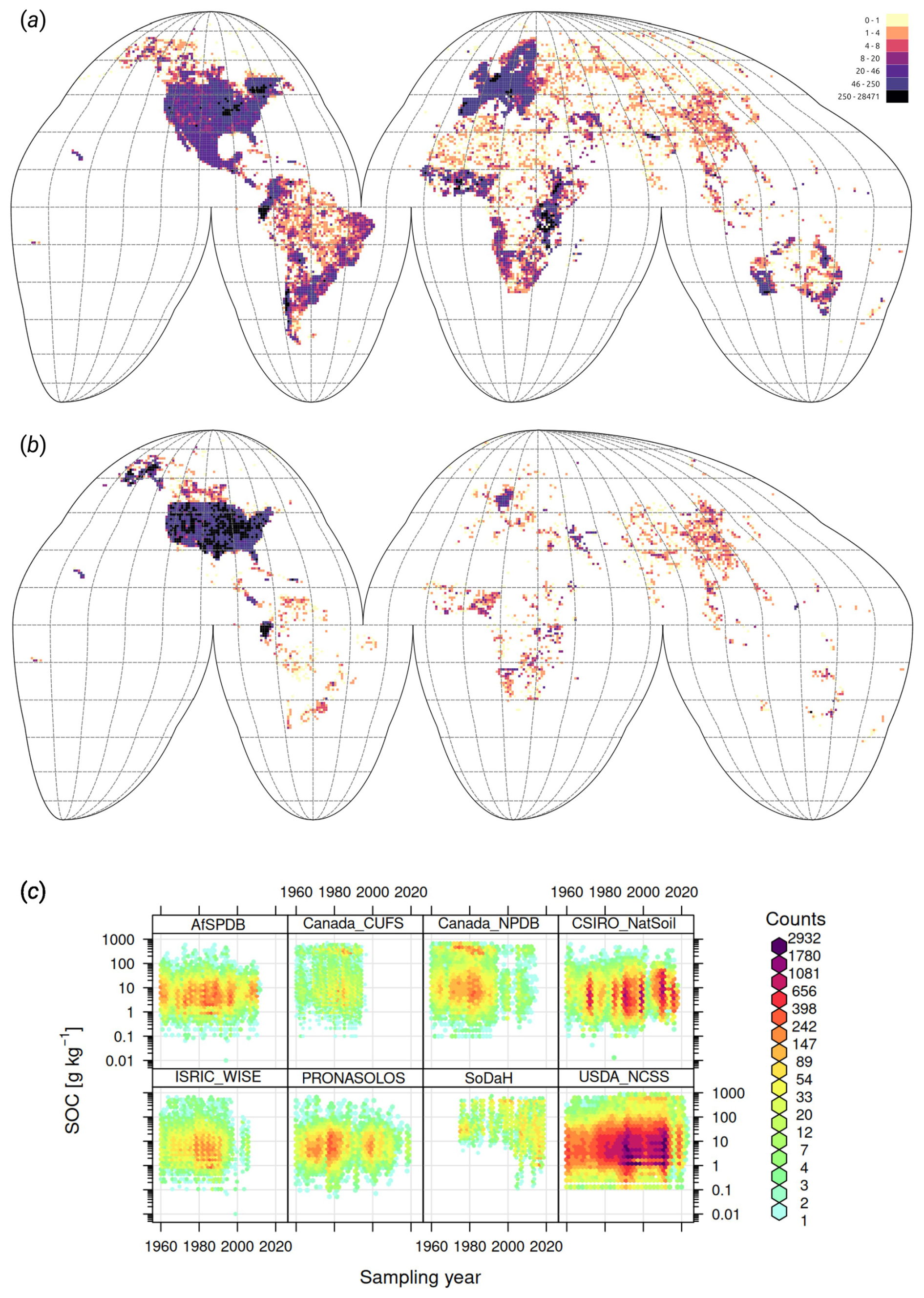
Figure 6 Density of training points used to build global predictive mapping models, and quality control plots for a number of key variables: (a) soil samples with soil organic carbon and/or soil pH, (b) soil profiles with soil taxonomy class, and (c) temporal coverage of samples from several larger datasets. Only points collected after year 1999 were used for modeling soil properties. For soil type mapping and to match high resolution covariates, we prioritize using points that are collected with GPS accuracy.

The final density of the training points prepared for the soil carbon, pH, soil texture fraction, and soil type mapping is shown in Fig. 6. Compared to some previous global modeling attempts (Poggio et al., 2021; Padarian et al., 2022b), our training data is harmonized to a single standard, e.g., DC method for SOC and try to equally represent the diversity of biomes and land use systems: from agricultural soils, forests, and specific biomes such as tropical peatlands to mangrove forests. The final harmonized points are available via https://soildb.openlandmap.org (last access: 6 June 2025) (the publicly available data; exclude LUCAS soil samples and similar) and will be continuously updated.

3.2 Accuracy of soil properties predictions

Results of validation using the stratified test data (hold-out samples) show RMSE of 17.7 [kg m⁻³] (0.486 in log-scale) and CCC of 0.88 for SOC density, RMSE of 51.3 [g kg⁻¹] (0.574 in log-scale) and CCC of 0.87 for SOC content, RMSE of 0.15 [t m⁻³] and CCC of 0.92 for bulk density of fine-earth, RMSE of 0.51 and CCC of 0.91 for soil pH, RMSE of 8.4 % and CCC of 0.87 for soil clay content, RMSE of 9.9 % and CCC of 0.87 for soil silt content, and RMSE of 12.6 % and CCC of 0.84 for soil sand content respectively. These accuracy levels match or exceed the accuracy levels reported in Poggio et al. (2021). Our predictions appear to be potentially more accurate for soil pH (our results RMSE 0.51 vs. 0.77), bulk density (our results RMSE 0.15 vs. 0.19), and texture fractions (our results RMSE 8.4 % vs. 13 % for clay content). Note that RMSE as an accuracy metric for log-normal/skewed variables is of limited use and probably should be avoided as RMSE is highly sensitive on few high values (e.g., organic soils); hence we are not able to compare our results to the results from SoilGrids V2 for SOC content. Based on the D² metric (distribution independent), the best performing variables appear to be soil pH, bulk density, and texture fractions, but all numbers are in principle comparable and in the range 0.70–0.85 for the holdout samples. We recommend to other groups to also report their D² metric as this seems to be distribution-independent; in the case of log-normal variables, we recommend estimating RMSE also in the log-space (natural logarithm).

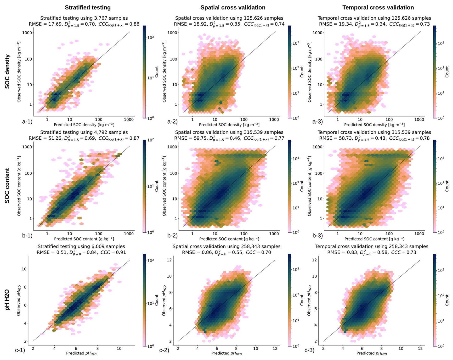
Figure 7 Accuracy plots for (a) soil organic carbon density [kg m⁻³], (b) soil organic carbon content [g kg⁻¹], and (c) soil pH H₂O based on the (left) stratified testing set, (center) spatial cross-validation, and (right) temporal cross-validation (LOYO). CCC for SOC density and content are derived in log-scale; RMSE based on stratified testing for SOC density and SOC content in log-scale is 0.486 and 0.574 respectively.

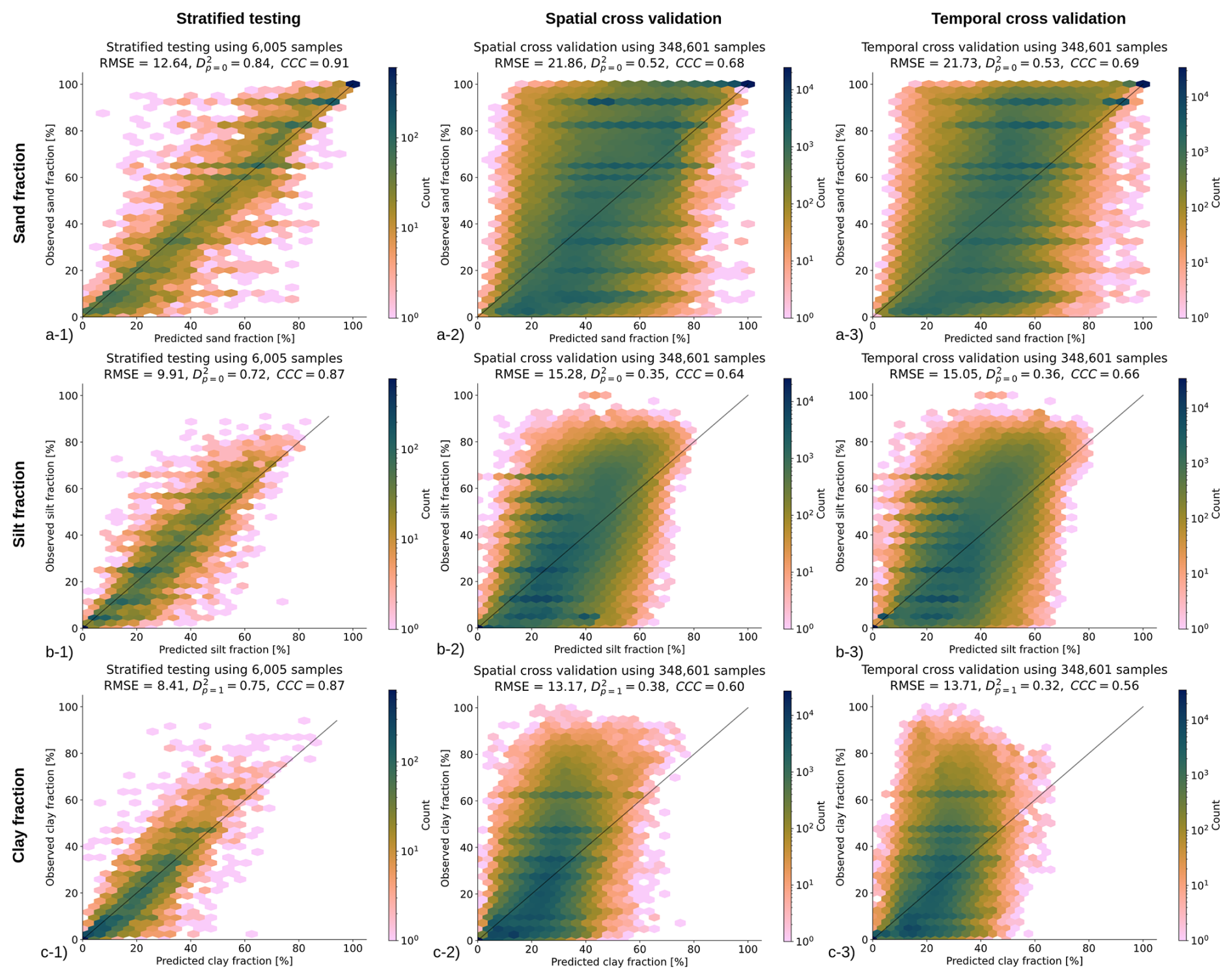
Figure 8 Accuracy plots for (a) sand fraction [%], (b) silt fraction [%], and (c) clay fraction [%] based on the (left) stratified testing set, (center) spatial cross-validation, and (right) temporal cross-validation (LOYO).

The PICPs for the target prediction interval (68 %) for the SOC density, SOC content, bulk density, and pH models are, respectively, 63 %, 67 %, 38 % and 57 %. While for SOC density and content the values are quite close to the ideal scenario, pH and in particular bulk density, the PICPs are quite smaller than the target PI. This motivated us to also check the quantile coverage probability (QCP), from which we can see that for the pH, the difference is reasonable and symmetrically deriving from upper and lower quantiles. For bulk density instead, the lower density is drastically off, and only converging to good performance around PI 90 %. In future versions, we can focus on improving the PICP for bulk density and predicting bulk density in space-time. Finally, the PICPs for texture fractions are 57 %, 64 % and 57 % for sand, silt and clay, respectively.

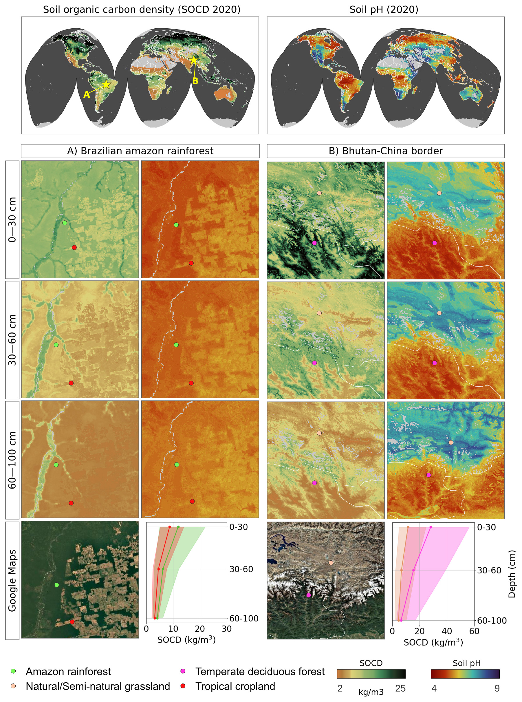
Figure 9 Predicted soil organic carbon and soil pH at 30 m resolution with zoom-in on two sample areas, with corresponding satellite images from Map data © 2025 Google. Soil-depth plots indicate 68 % probability prediction intervals based on the Quantile Regression Random Forest.

The accuracy results for different validation strategies are shown in Fig. 7. These show a clear difference between stratified testing and spatial CV (with blocking), which was also expected. In general, we consider that temporal and spatial CV give the most pessimistic accuracy results and stratified testing gives independent results, but because we do not really have a probability sample, we consider these results potentially over-optimistic. For example, for predicting SOC density, CCC is between 0.73–0.88; for soil pH, the RMSE is between 0.51 and 0.83. The difference in D² for all variables between stratified hold-outs and spatial blocking appears to be the largest, with values for SOC density, for example, ranging between 0.68–0.84. It is interesting to observe that the temporal CV achieves accuracy similar to that of the spatial CV indicating that indeed models fitted over a longer period of years (25+ years) can be used to predict also new years e.g. 2025, 2026 for which we maybe have no new training points. The predicted soil property maps also show very gentle changes, with most pixels (>90 %) not changing much from period to period.

Table 1 Model performance for SOCd, SOC content, BD, and pH${}_{{\mathrm{H}}_{\mathrm{2}}\mathrm{O}}$ across different depth intervals, calculated on the testing set. The values signed with ^* are computed in the log (1+x) space, as illustrated in Fig. 7. Note that “All points” can include also points that are deeper then 100 cm.

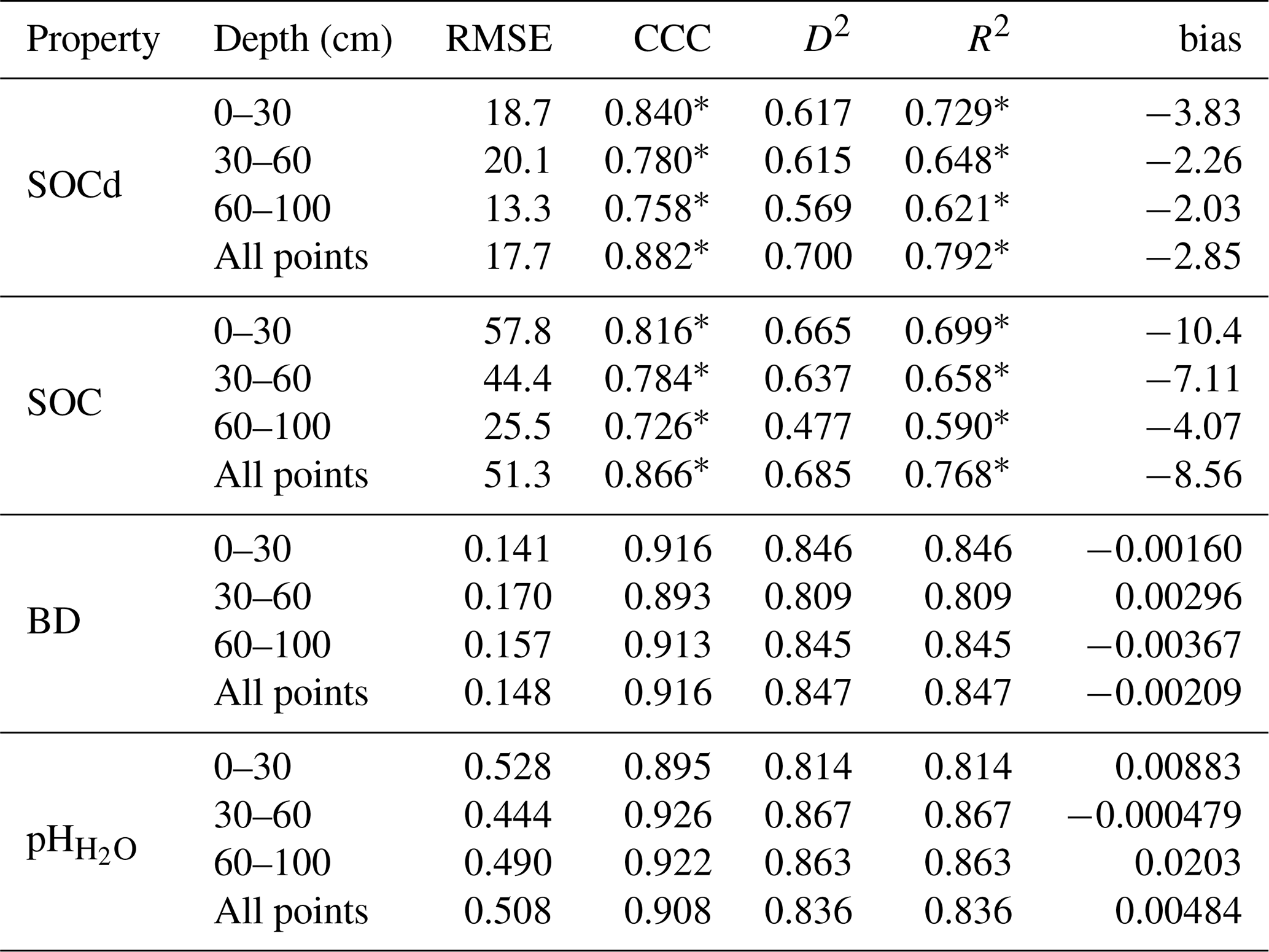
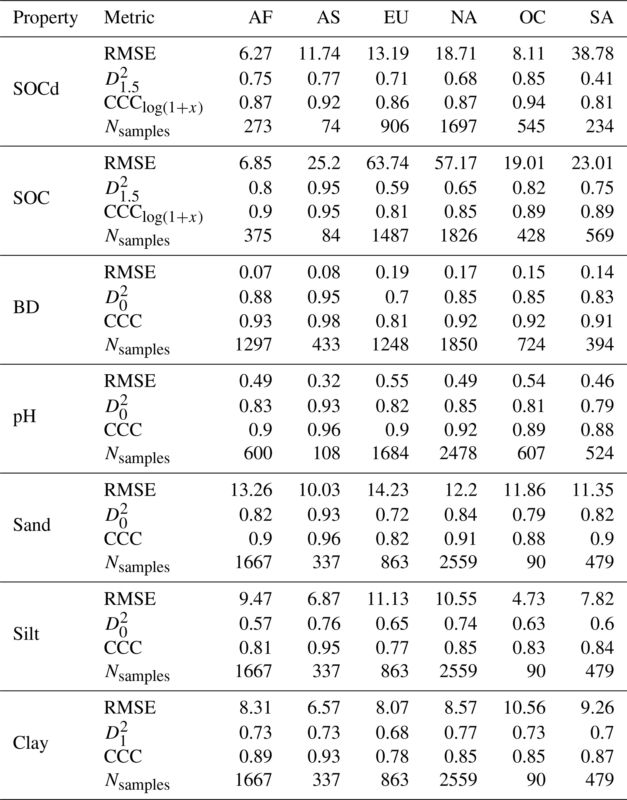
Table 1 shows the results of the accuracy assessment for the target soil properties for different standard depths: 0–30, 30–60 and 60–100 cm. These results indicate that, as expected, the highest accuracies for SOC density and content are achieved for the top soil: CCC drops from 0.84 to 0.76 going from 0–30 to 60–100 cm. However, the difference in accuracy between depths in our results appears to be in general minor, with most values oscillating ± 5–10 % between different depths (Table 1). This is a somewhat unexpected result, although for SOC density and similar the values at higher depth are also significantly lower, so possibly this is why the errors are also in average lower even though models are typically based on much fewer points than what is available for top-soil. Table 2 shows differences in accuracy for different continents based on Equi7grid zones (6 continents) (Bauer-Marschallinger et al., 2014). On average, CCC seems to be comparable with no continent performing significantly worse. It seems that Asia shows the most accurate predictions, although there also seem to be significantly less points available for that continent, hence this over-performance might just be effect of low density of points.

Table 2 Model performance for SOCd, SOC content, BD, and pH${}_{{\mathrm{H}}_{\mathrm{2}}\mathrm{O}}$, Sand, Silt and Clay across different continents (AF = Africa, AS = Asia, EU = Europe, NA = North America, OC = Oceania, SA = South America). Compare with Table 1.

Our results of cross-validation also show some bias in predicting SOC content and SOC density and clay content, with our models potentially over-predicting smaller SOC values and under-predicting higher clay content. This indicates that it is important to use prediction intervals (we provide lower and upper prediction intervals as maps as shown in Fig. 9) together with predictions to incorporate the uncertainty of these models.

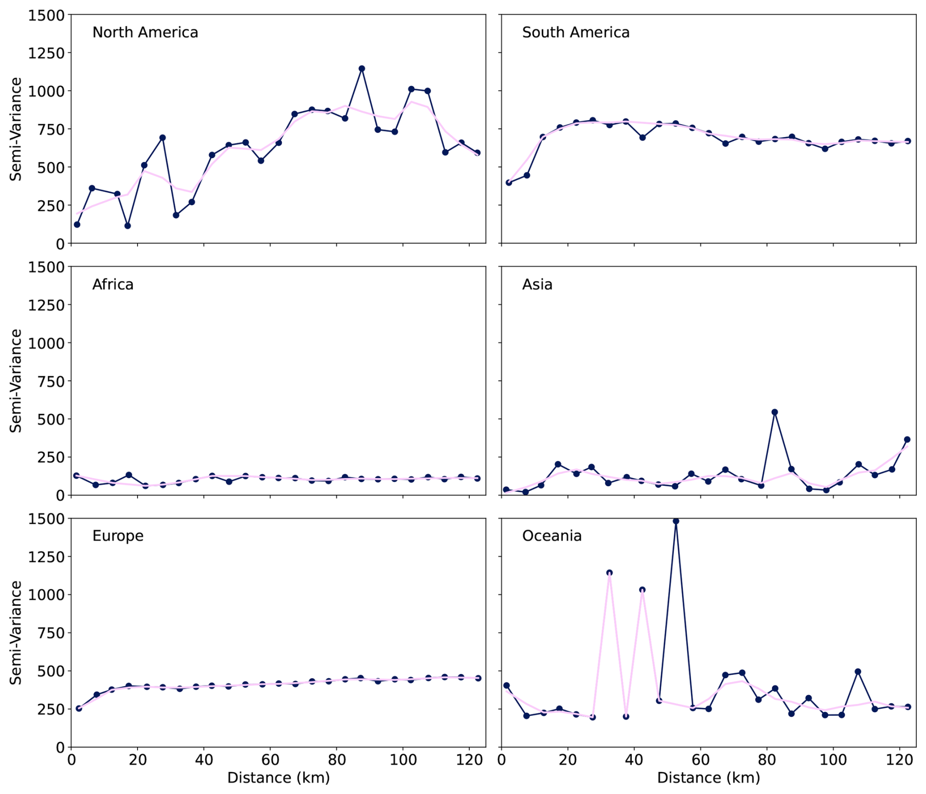
Figure 10 Sample semi-variograms of SOCd prediction residuals across six continents (10-fold CV), with distances computed using continent-specific equal-area projections. Binned every 5 km up to 125 km (dark blue dots an line), smoothed by LOWESS (pink). GLanCE points (pseudo-observations) were excluded.

Semivariograms representing spatial autocorrelation of model residuals for SOCd are shown in Fig. 10. Except for North America, residuals show either no spatial autocorrelation structure or spatial dependence at shorter distances, i.e. up to maximum 10–20 km. Considering that only a fraction of the points are available at distances of < 10 km. We hence do not consider kriging of residuals for these data, although for further merging with local data combining variogram modeling with RF could help increase accuracy.

3.3 Key covariates explaining global distribution of targeted soil variables

The results of variable importance for the soil variables of interest are shown in Fig. 11. For SOC density, it is especially interesting to see that Landsat-derived GPP (30 m resolution, bimonthly aggregated to annual) comes in the top three most important covariates (see R1). Conceptually speaking, we expect that primary productivity is the key source of SOC, at least in natural vegetation systems. As expected, depth explains almost 30 % of variability in the SOC distribution and is distinctly at the top, which justifies the use of soil depth as a covariate.

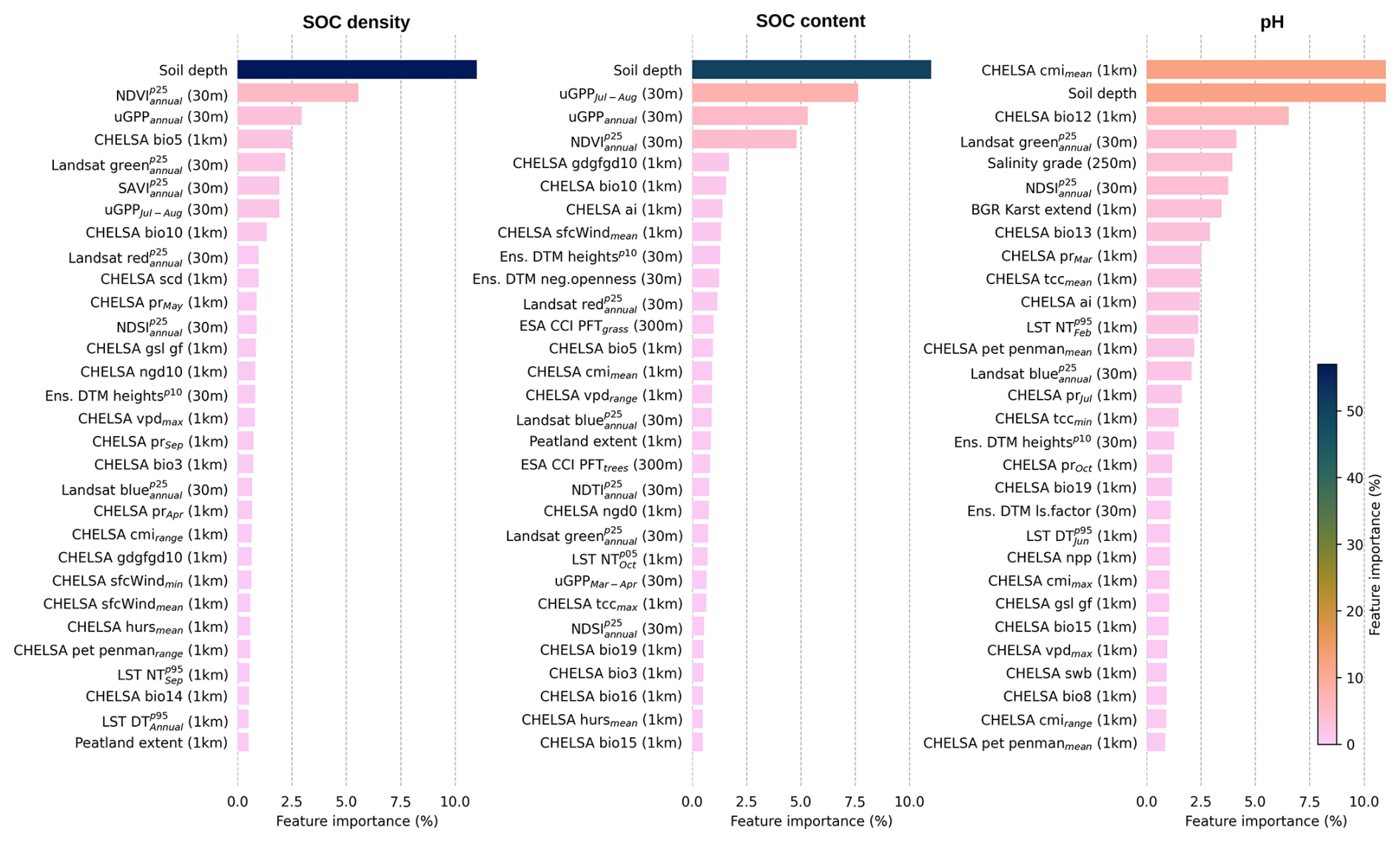
Figure 11 Variable importance plots for soil organic carbon density, soil organic carbon content, and soil pH.

The global distribution of soil pH can be primarily explained by the CHELSA Aridity Index (long-term), annual precipitation, and the grade of salinity (Ivushkin et al., 2019). The correlation plots in Fig. 12 show how the top 4 most important variables listed for the SOC density correlate with each other as shown using 1:1 density plots: higher GPP/higher vegetation index and cooler climates convert to higher SOC. SOC density and soil depth are close to linearly correlated on a log-log scale, as are SOC density and GPP. This also illustrates that the uncertainty of individual driving factors is still relatively high.

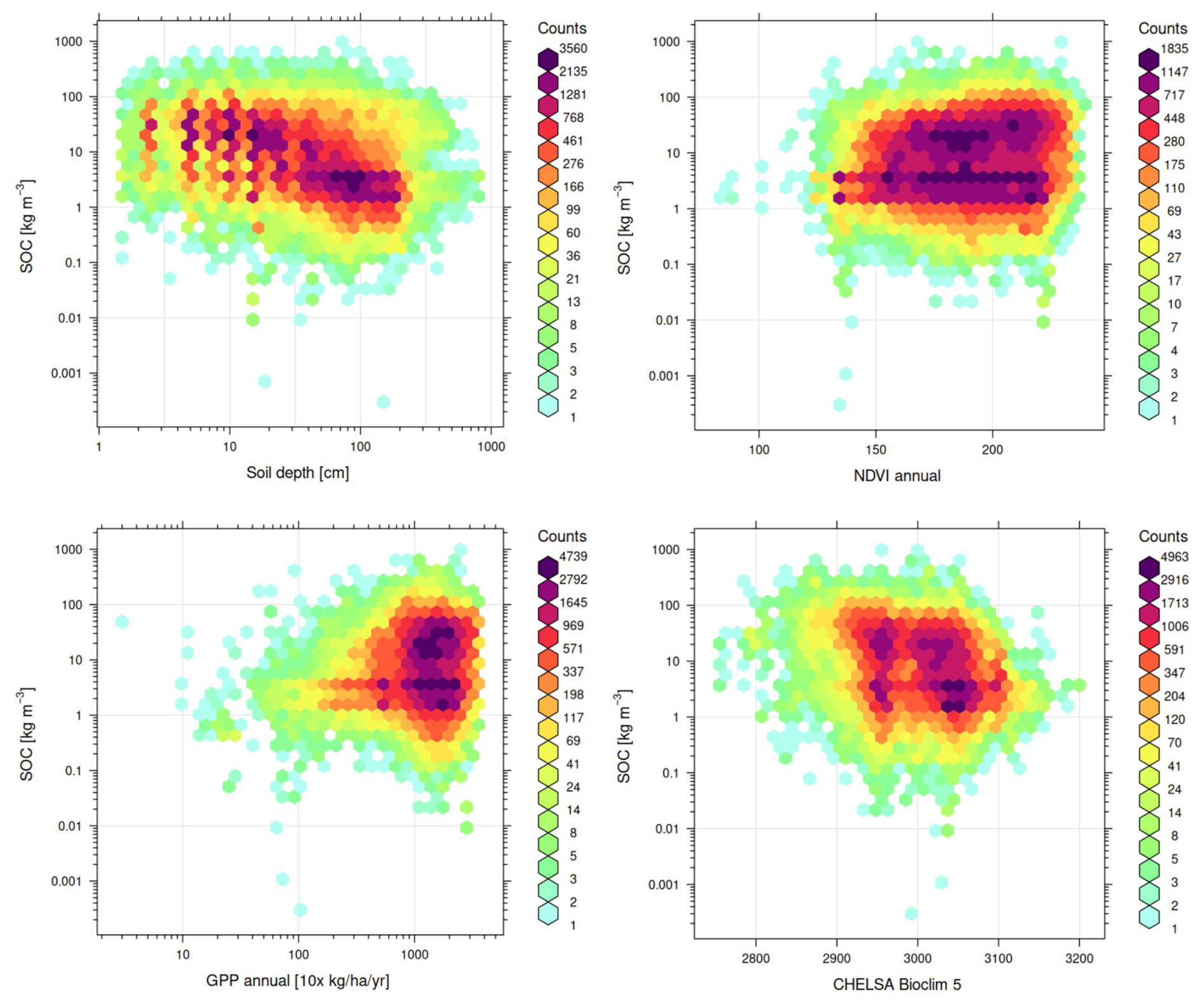
Figure 12 Scatterplots for the top 4 most important variables for modeling SOC density. GPP = annual Gross Primary Productivity based on Landsat; NDVI = Normalized Difference Vegetation Index (0–255 values); CHELSA Bioclim 5 = the highest temperature of any monthly daily mean maximum temperature.

3.4 Accuracy of soil type predictions

The results of the accuracy assessment using spatial blocking for the soil subgroups (818) show that, as expected for this high number of classes, the F₁ score does not exceed 0.30. We observed log loss of 2.49, 2.74 and 2.46 for RF, LightGBM and the ensemble model; and a F₁ score of 0.23, 0.30 and 0.30 respectively. Overall, the ensemble model seems to be justified, although the difference in accuracy is marginal.

Figure 13 shows the 30 most important variables for the RF and LGB ML models displayed together. The features are sorted in descending order according to the importance values of the LightGBM model. This indicates that both models agree with each other in terms of important features, but there are changes in the order. Elevation (GEDTM30) seems to be the most important feature in both models. In general, climate variables from the CHELSA product at 1 km spatial resolution dominate the list of important features.

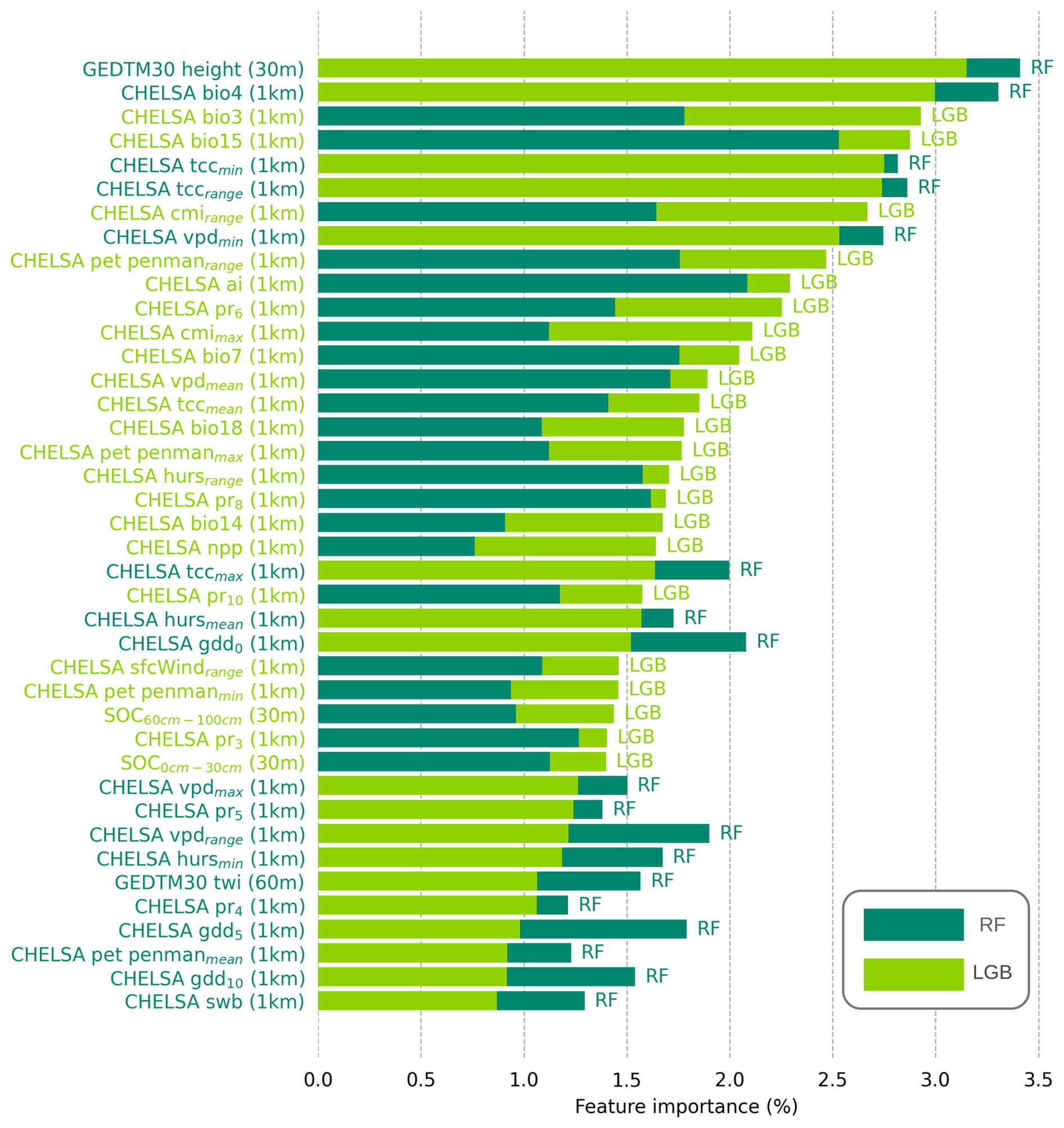
Figure 13 Variable importance plots for soil type mapping using RF and LGB models. Labels are colored based on the model (RF or LGB) that assigned the highest importance to each feature.

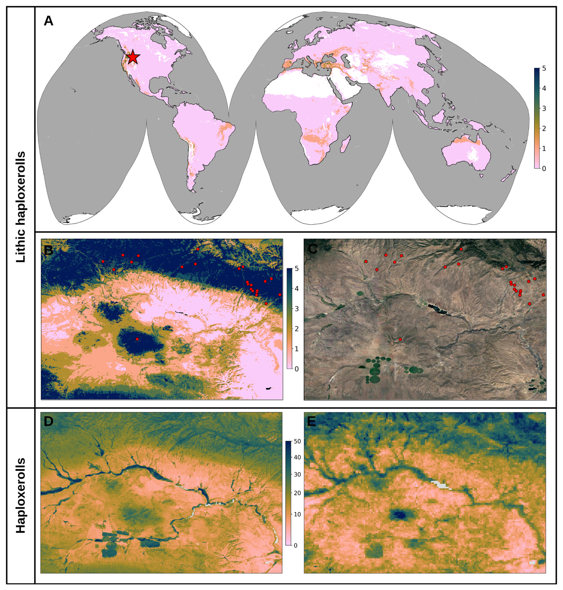
Figure 14 Example probability maps of soil types: (a) Global probability of Lithic Haploxerolls, (b) Regional probability of Lithic Haploxerolls in the area marked with a red star in the USA in (a), (c) Map data © 2025 Google of the same region, (d) Aggregated probability of all Haploxerolls, and (e) Probability of Haploxerolls from OpenLandMap 2018 map at 250 m resolution. Lithic haploxerolls training points are shown as red circles in (a) and (b). Note: the probability maps for Lithic Haploxerolls and aggregated Haploxerolls shown use different legends – the legend for 250 m predictions have been adjusted to achieve similar contrast.

Figure 14 shows an example of soil type prediction maps for Lithic Haploxerolls. The global map reveals places where Lithic Haploxerolls are more probable, especially in North America, the Mediterranean, and central Asia. For a more detailed view, we focused on a small area to illustrate the small-scale variations compared to the land features depicted in the satellite imagery. We compared the probability maps with the OpenLandMap probability maps at 250 m resolution from 2018 (https://doi.org/10.5281/zenodo.1476844, Hengl and Nauman, 2018). Since OpenLandMap 2018 does not include soil subgroups, in this case Lithic Haploxerolls, we aggregated all Haploxeroll subgroups in our map to generate a comparable probability layer (see Fig. 14d). Overall, the increase in spatial detail is a positive result: predictions help detect many local features, and could be potentially used for farm-scale decisions. However, it is difficult to know how well these predictions match the true patterns in soil polypedons in the field.

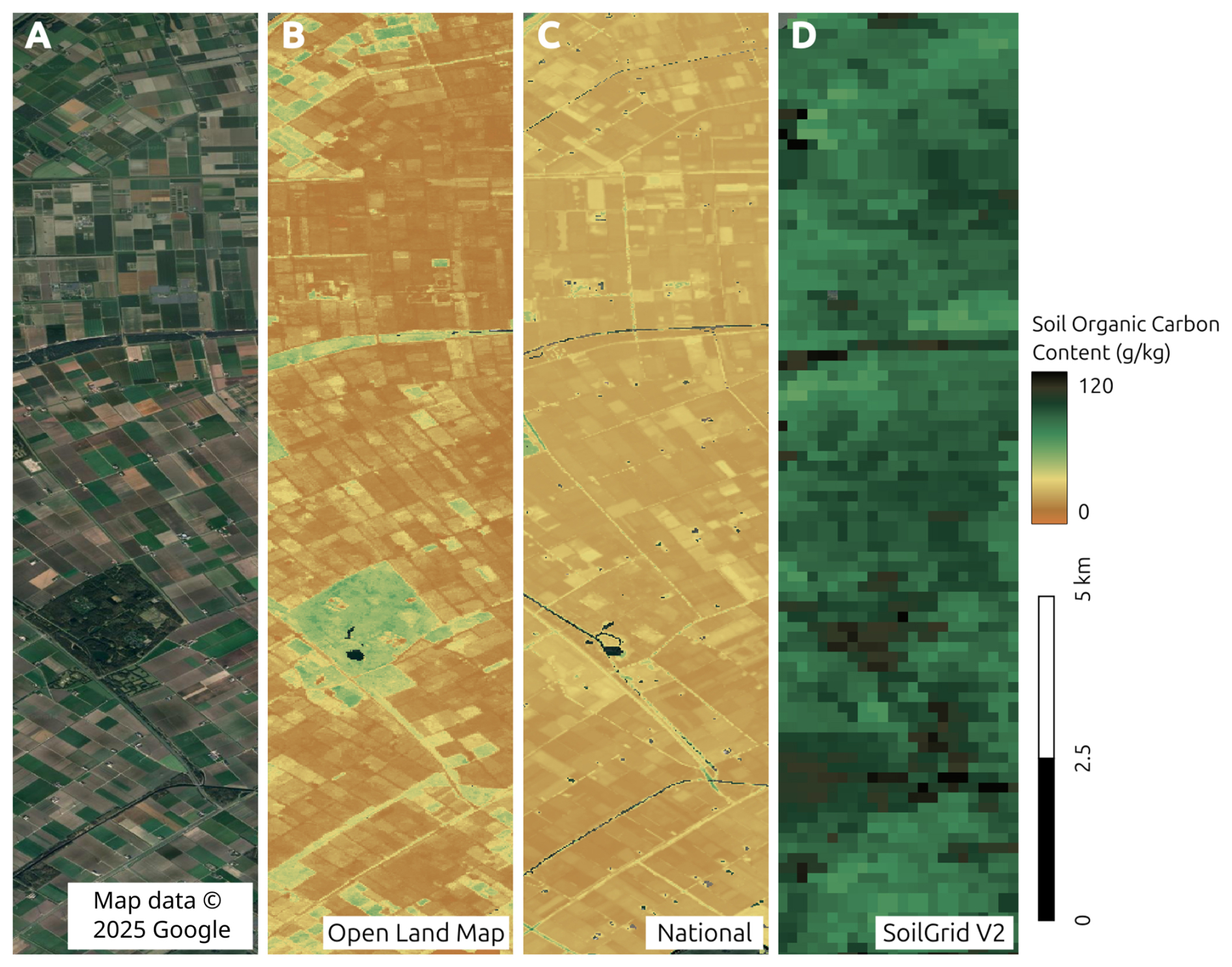
Figure 15 Comparison between SOC content maps of the region in the Netherlands, based on: (A) satellite imagery from Map data © 2025 Google; (B) our model predictions for the 2020–2021 period (0–30 cm depth, 30 m resolution). (C) locally generated national SOC maps (0–5 cm depth, 25 m resolution, converted from SOM) for the year 2020, produced by Helfenstein et al. (2024); (D) SoilGrids V2 data (0–5 cm depth, 250 m resolution) released in 2020 (Poggio et al., 2021).

3.5 Comparison with other similar global data sets

Figure 15 shows the difference in spatial detail and general patterns for an area in Germany. This illustrates the difference between 30 and 250 m spatial resolution, which in a case of managed land can be drastic with 250 m completely missing field boundaries and patterns within the field. The SOC content predictions from SoilGrids V2 seem to overpredict the SOC values by a factor of 2–3 times, which is a known problem with SOC predictions where models have limited accuracy and most of low values are over-predicted. Note that it is not easy to compare all possible SOC and pH maps as our predictions relate to specific time intervals (e.g. 2000–2005), while many soil mapping products ignore time-dimension.

In the case of soil texture fractions, bulk density, coarse fragments, and clay mineralogy, there is probably no need to map these at shorter time intervals, e.g. < 20 years. In the case of chemical soil properties, our results show that differences (changes) will be visible at 5 year intervals, although in general changes in all soil properties are relatively minor (gradual), and users need to carefully look and zoom in to notice any changes.

In general, the investment in processing global 30 m resolution data seems to be paying off, and the spatial detail of our predictions is comparable to that of Helfenstein et al. (2024). The differences between our predictions and national predictions open an opportunity for further local-global data fusion. Some ideas on how to implement this are mentioned further in the discussion section.

3.6 Detected trends in soil organic carbon density and soil pH

Based on the predictions, we also derived changes in soil properties corresponding to land cover transitions using the sampled point data set. The distributions of the SOCd and pH changes between 2000 and 2022+ across the most prominent land cover change classes are visualized in Fig. 16. In general, both SOCd and pH exhibit decreasing trends for these change classes. Transitions involving tree loss such as “Tree cover broadleaved evergreen ↦ Mosaic cropland or natural vegetation” (TREBE-MCRNV), “Tree cover broadleaved deciduous ↦ Mosaic cropland or natural vegetation” (TREBD-MCRNV), “Tree cover broadleaved deciduous ↦ Cropland rainfed” (TREBD-CRPRF), “Tree cover needleleaved deciduous ↦ Mosaic tree and shrub or herbaceous cover” (TREND-MTSHH) and “Tree cover needleleaved evergreen ↦ Grassland” (TRENE-GRASS), are associated with stronger negative trends in SOCd.

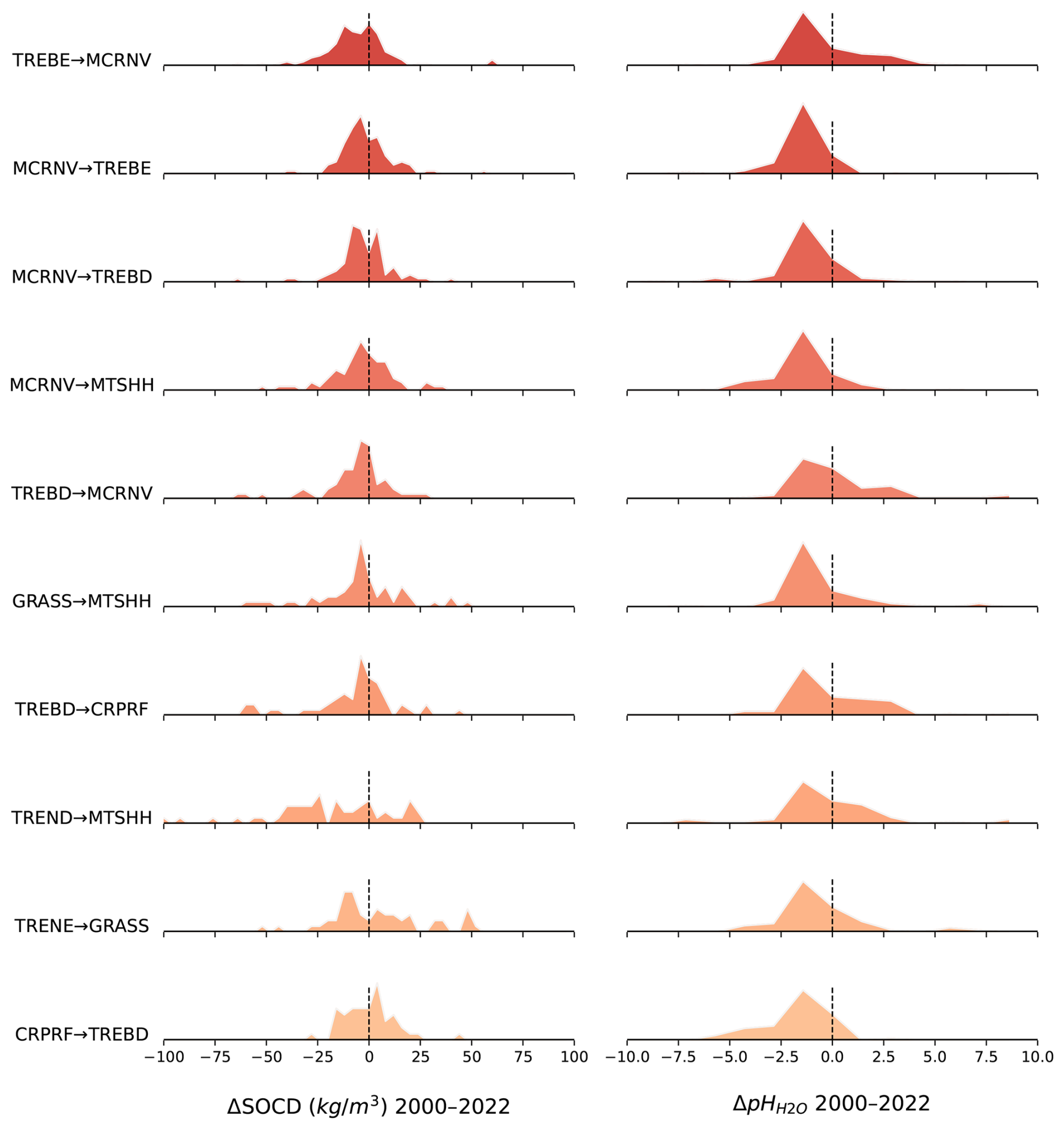
Figure 16 Distribution of soil property changes from 2000–2005 to 2020–2022+ (ridgeline plots; left: SOCd, right: pH) across the top 10 most frequent land cover change classes. TREBE – Tree cover broadleaved evergreen; MCRNV – Mosaic cropland or natural vegetation; TREBD – Tree cover broadleaved deciduous; MTSHH – Mosaic tree and shrub or herbaceous cover; GRASS – Grassland; CRPRF – Cropland rainfed; TREND – Tree cover needleleaved deciduous; TRENE – Tree cover needleleaved evergreen. The intensity of the color indicates the relative density (frequency) of occurrences for each land cover change class within the sampled dataset.

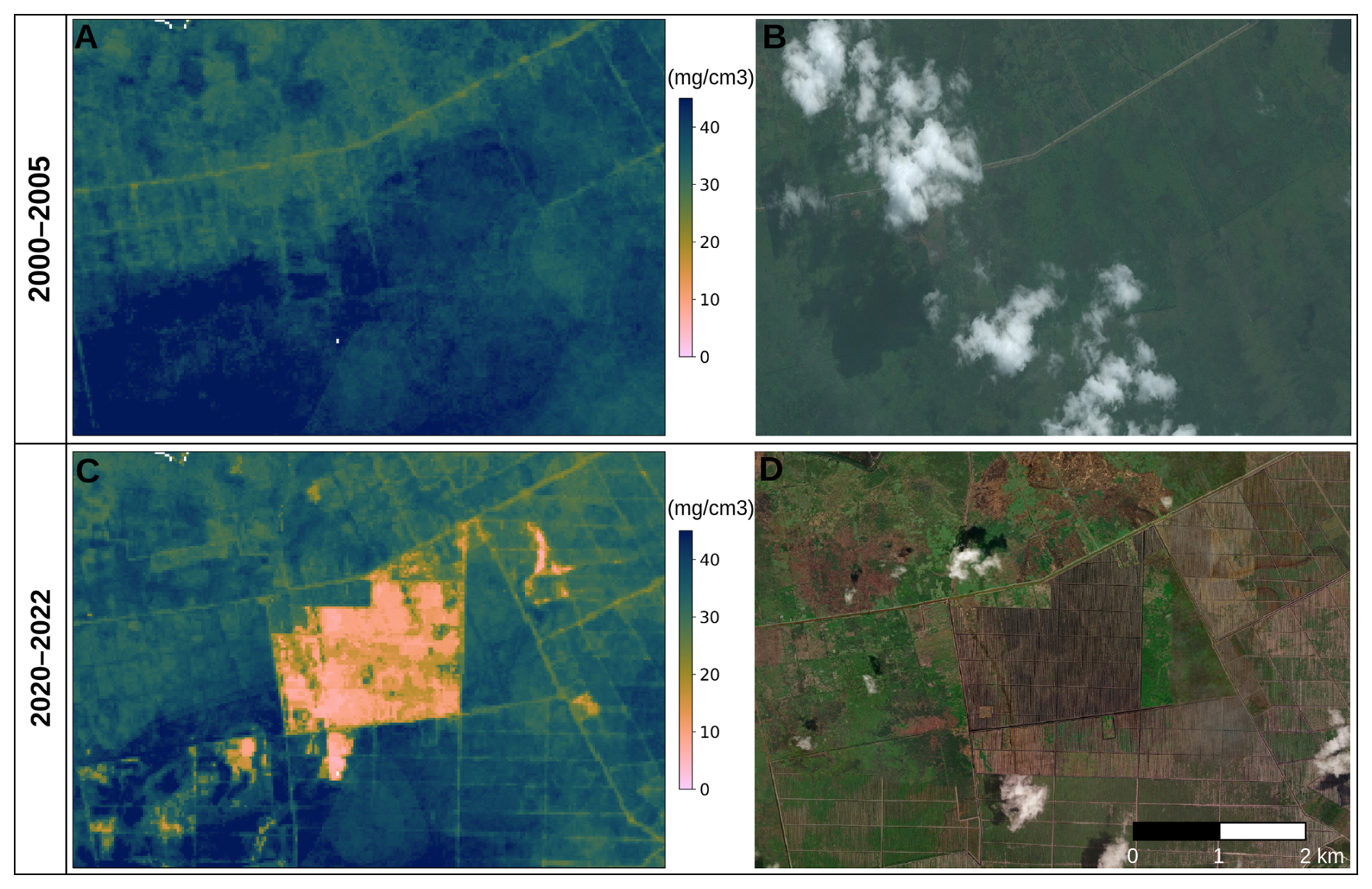
Figure 17 Comparison predictions of SOC density for 2000–2005 and 2020–2022 periods for area in Indonesia. (A) SOCd map for the period 2000–2005, (B) Satellite imagery from 2014 (Powered by Esri), indicating largely intact forest cover, (C) SOCd map for the period 2020–2022, and (D) ESRI satellite imagery from 2022, revealing extensive clearing and agricultural conversion.

Table 3 Total carbon stocks (Pg) by period and soil depth.

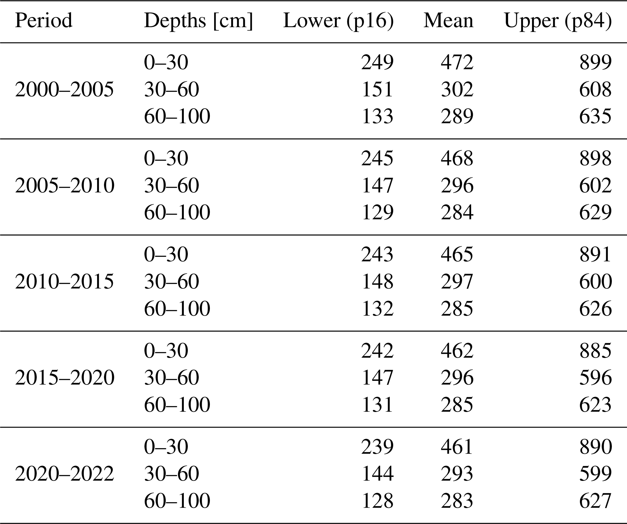
These results align with the findings that SOC loss in the tropics is largely driven by deforestation (Fig. 17), although increasing droughts and forest fires could also be the main driver of this trend (Naval et al., 2025). For other land cover transitions, the decrease in SOCd is less pronounced. Changes in pH exhibit a relatively uniform distribution in all examined land cover change classes, with a slight trend toward acidification. We finally estimate that the world has lost 11 Pg of SOC from 2000 to 2022 based on these results. Note that, due to the limited availability of training data, especially for the Russian Federation, the actual loss of SOC could be even higher.

4 Discussion

4.1 Summary findings

We implemented a High Performance Computing system (EO-SoilMapper) to map dynamic soil properties at multiple depths (0–30, 30–60 and 60–100 cm) over time (5-year intervals from 2000–2022+) and with uncertainty quantified per pixel. This allowed us to produce complete, consistent and current predictions of some key soil properties such as SOC content, SOC density, soil pH, and soil types at unprecedented spatial resolution. We refer to this data set as the “OpenLandMap-soildb”. Our ambition is to continuously update, expand and improve these data to serve the global good, especially to support projects such as the United Nations Convention to Combat Desertification (UNCCD), Land Degradation Neutrality, open source carbon accounting, and soil health monitoring across borders.

We evaluated the accuracy of prediction models using stratified testing based on climate zones, 5-fold spatial blocking cross-validation, and LOYO using best quality data. The results show improvements in terms of spatial detail (Fig. 15) and accuracy (Fig. 7) for SOC content, SOC density, and soil pH, compared to previous global soil mapping initiatives (Hengl et al., 2017; Poggio et al., 2021). Having a time-series of predictions based on a single model allows comparing changes over time, which is especially interesting when it comes to tracking chemical soil properties such as SOC and soil pH (Fig. 16). The loss of carbon density is known to be related to land degradation, which often begins with deforestation, draining of wetlands, and similar. Naval et al. (2025) found that annual forest burning depletes soil C stocks (0–30 cm) by 16 %, triennial burning by 19 %, and long-term agriculture by 38 % (compared to undisturbed forest in the tropics). Our results show that the SOC losses for the last 25+ years are primarily driven by deforestation and the removal of peatlands.

These results of the accuracy assessment confirm that the time invested in preparing these data at high spatial resolution (30 m) was worthwhile. This required significant efforts to prepare and fine-tune the training data and input covariate layers, in addition to the technical challenges of processing these data in a cost-effective way. It was especially tedious to import and bind all national and international soil laboratory measurements and observations into a single analysis-ready training data set. Laboratory soil data are often only available in parts and without any standard schema: to fully document all harmonization steps can be extremely lengthy, and eventually we had to often make expert decisions, resulting in the extensive code-base provided at https://soildb.openlandmap.org. We will continue to extend this data and make the process transparent/open source.

We have released all the data produced as open data (CC-BY license), available via an interactive app at https://world.soils.app (last access: 6 June 2025), and have exposed our workflows currently implemented via the scikit-map package calling for the establishment of open development communities, comparable to the Open Soil Spectral Library (Safanelli et al., 2025), to help maintain and improve these data. In the next sections, we discuss limitations of the data, suggest some recommended uses of them, and envision future development directions.

4.2 Towards a more accurate estimate of soil dynamics

One of the significant results of this work is that we have been able to estimate SOC stocks based on detailed SOC density maps. Our results show (Table 3) the global stocks for each spatio-temporal block. For example, the carbon stock for the 0–30 cm depth interval in the most recent time-frame (2020–2022+) is estimated to be 461 Pg (Peta grams) for 114 million km² (excluding Antarctica, Greenland, deserts, and permanent ice/snow) with a 68 % probability range of 239–890 Pg. We further estimate that the total stocks for 0–1 m of the soil depth is 1037 Pg. This number is somewhat higher than what is reported by Padarian et al. (2022b), but also significantly less than what several other sources suggest (Jackson et al., 2017; Lin et al., 2022).

The significant amount of SOC in our predictions in the subsoil is mainly contributed to the northern hemisphere and tropical peatlands. In the rest of the world, deeper soils typically contain only a fraction of the total SOC e.g. 10 %–15 % of the total stock for 30–200 cm. Our predictions of high SOC stocks for northern latitudes (>55°) should be taken with caution, as we had limited training data for Russia. Our predictions for northern latitudes are likely based on two main data sources: the Northern Circumpolar Soil Carbon Database (NCSCD) (Hugelius et al., 2013b) and the Interior Alaska Carbon and Nitrogen stocks (Manies et al., 2020). These data sets appear to represent northern peatlands and wetlands with obvious right skewness toward high SOC density (Fig. 18). Most of the literature agrees that most SOC stocks in the world belong practically to Canada and the Russian Federation (Scharlemann et al., 2014; Crowther et al., 2016). We now provide predictions of SOC density at high spatial detail. An important note here is that many of the tundra and taiga areas of the world, although probably have a high SOC content, are also shallow soils with a significant amount of coarse fragments. Although we corrected for coarse fragments during the derivation of the SOC content, many soil profiles do not report coarse fragmentation, so the actual stocks we estimated could be somewhat lower in fact. We plan to add coarse fragments, depth to bedrock, and similar to the list of variables for global soil mapping in the next update. Many soil properties are, in fact, (quasi-)static e.g. clay mineralogy, lithology and parent material, also bulk density and similar do not change even at a scale of few hundred years, and hence need only high quality long-term estimates. The bulk density (BD) of the fine-earth fraction, however, is controlled by SOC content; thus, because SOC changes, we can assume that BD might also change and hence need to be also mapped in spacetime.

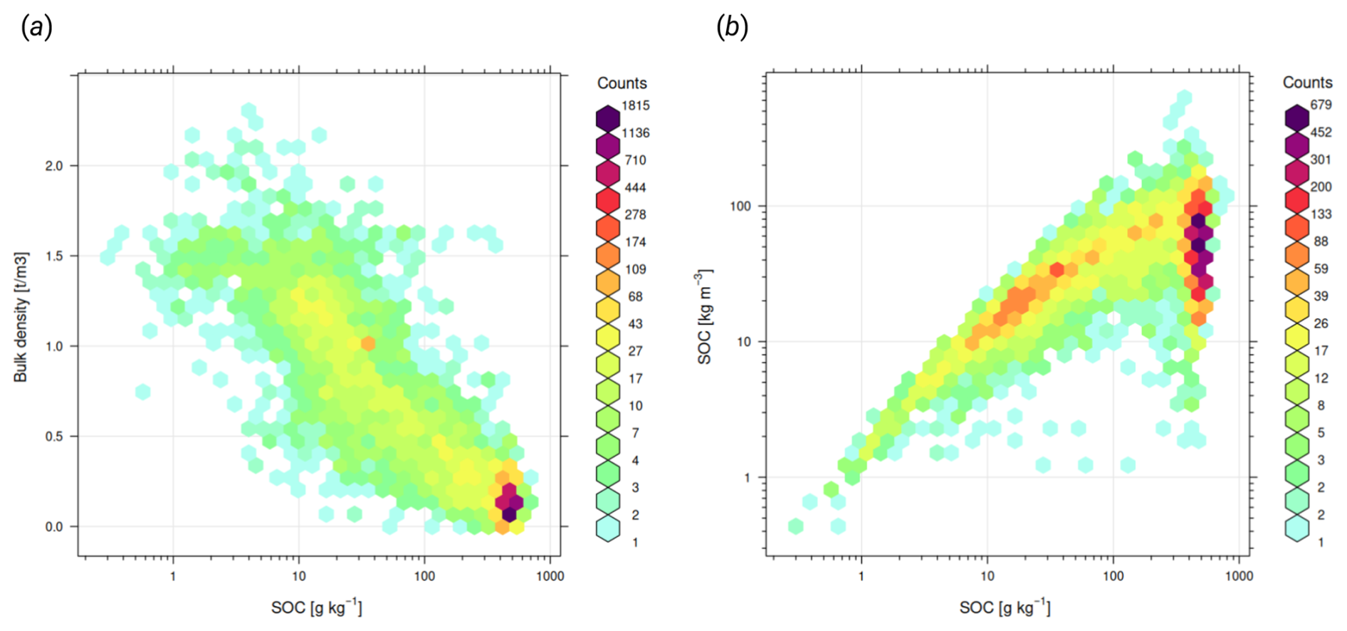
Figure 18 Density plot showing: (a) relationship between SOC density and Bulk Density (fine-earth), and (b) SOC content and SOC density based on the Northern Circumpolar Soil Carbon Database (NCSCD) (Hugelius et al., 2013b). The right figure shows how the main source of uncertainty in SOC stock estimates for the world are likely the high variation in the the stocks for soils with > 10 % of SOC.

Our results further show that the planet has lost at least 11 Pg of SOC for 0–30 cm in the period 2000–2022+. We think that this is probably a conservative estimate as our models possibly smooth out and also miss especially some peatlands in the tropics. It is important to note that this number is derived directly from the data. We make no assumptions or apply change functions that represent the processes and/or drivers of the SOC change (e.g. Padarian et al., 2022b). We hope to improve this estimate with each new update of the predictions, which will hopefully be driven mainly by the addition of more and higher quality training points.

4.3 The OpenLandMap approach to global soil mapping

Having a 30 m resolution data product means that the state-of-the-art global soil mapping is on a path to becoming compatible (in terms of spatial detail, consistency, and completeness) with high-resolution global layers such as land cover (Potapov et al., 2020), cereal extent (Van Tricht et al., 2023), forest canopy (Turubanova et al., 2023), and similar. Our predictions span almost 25 years and therefore can be used to detect changes, i.e. this is now potentially a farm-scale, decision-ready geospatial soil database. Our trend analysis based on space-time predictions visually shows that the decrease in SOC is correlated with deforestation, especially in countries rich in organic soils such as Indonesia (Fig. 17).

We model dynamic soil properties using a data fusion approach, that is, using an extensive combination of time series of EO-based biophysical indices, climatic variables, terrain variables, variables representing human impact, and using pseudo-observations to help incorporate soil knowledge into ML (Fig. 1). Compare with the approach of van Wesemael et al. (2024), for example, who decided to fit two separate models – one for areas with enough bare-soil spectra, one for areas permanently covered with vegetation such as grasslands and forests (bare-soil spectra are often only available for $\mathrm{1}/\mathrm{3}$ to $\mathrm{1}/\mathrm{2}$ of the land mask or less). In our opinion, direct use of bare-soil spectra, for example from Landsat or Sentinel optical images, although shown to be promising for mapping SOC in agricultural areas, seems to be applicable only for a narrow niche of mapping top soil in intensely managed agricultural soils. In our framework, we use instead a much denser number of long time-series of Landsat indices (bi-monthly to annual) to represent both bare surface and vegetated spectra. This makes our OpenLandMap-soildb global soil mapping approach an order of magnitude more computational, more hyper-dimensional than the approach of van Wesemael et al. (2024) and/or Fu et al. (2024), and this is probably a downside. On the other hand, the advantage of our approach is that we did not have to fit separate models, then fix boundary issues etc. Another disadvantage of our approach is that we underused the potential of extracting bare-surface soil spectra. In summary, using bare-earth soil spectra and using dense time-series of monthly/bimonthly spectral signatures (our approach) are both valid approaches and would need to be compared versus the same test data to objectively compare differences.

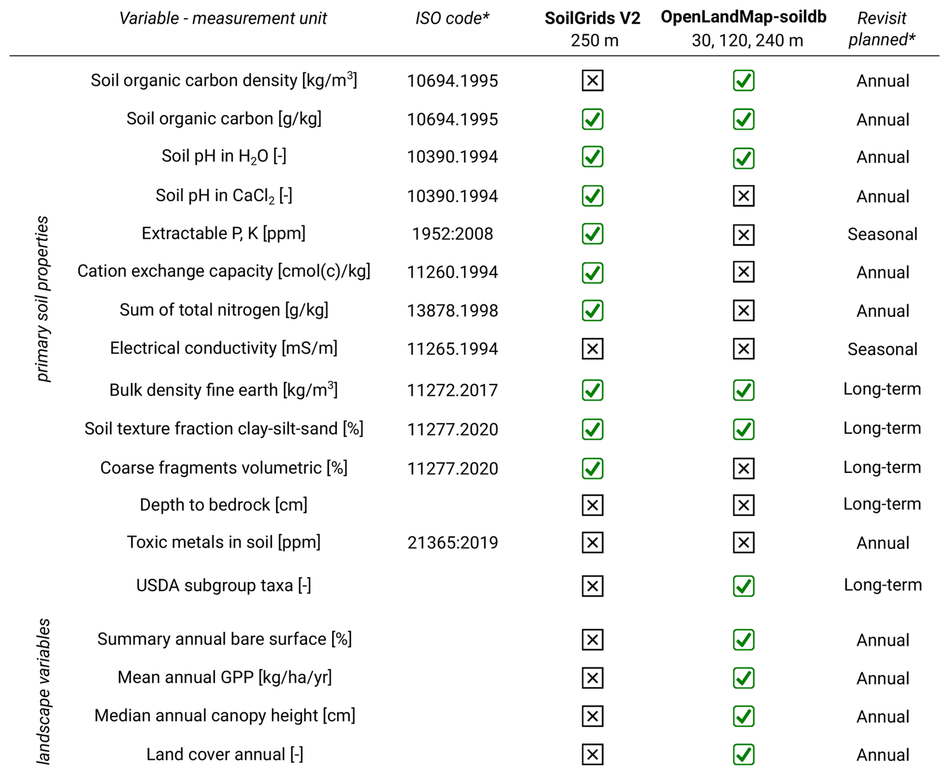
Figure 19 Primary soil properties of interest for global soil mapping (Chen et al., 2022), ISO code, temporal granularity and current availability in OpenLandMap-soildb. The ISO standard code is approximated. Toxic metals include: arsenic, cadmium, cobalt, chromium, copper, nickel, and lead.

From a personal perspective, the scale of the product, due to the 30 m/120 m spatial resolution, different timeframes and depths, quantiles and mean, and numerous properties, required a high computational effort. In general, the production phase required hundreds of thousands of CPU hours and resulted in more than 30 TB of output storage size. Consequently, we had to make compromises in terms of selection of properties and temporal resolution – currently we only map 5-year periods (averaged over 5-year blocks: 2000–2005, 2005–2010, 2010–2015, 2015–2020, 2020–2022+). For top soil SOC density we also produced a more granular product with overlapping biannual time-frames to be used as annual product in the range 2015–2022+. In addition, we originally wanted to also map coarse fragments, depth to bedrock, macro and micronutrients, and similar (Fig. 19), but these would have pushed us beyond the project budget. To illustrate data volumes, the world's land mask at 30 m is about 220 billion pixels (Ho et al., 2025), therefore, if we include multiple depths and uncertainty, only one time period for one soil property contains more than a trillion pixels. Some variables such as depth to bedrock have already been mapped (Shangguan et al., 2017), but only at coarse spatial resolution (1 km) and with limited accuracy. This is also because only limited training (point data) on depth to bedrock is available; depth to bedrock is also a so-called “censored variable” and might require special modeling framework to account for a large number of >200 cm values. Adding depth to bedrock, coarse fragment fraction, World Reference Base soil types, and similar are hence a high priority for the next updates.

The preparation, harmonization, and binding of points (training data) and the preparation of the covariate layers took almost 60 %–80 % of the OpenLandMap-soildb project time and was difficult to predict. Consider, for example, the peatland extent map of the world: currently, there are at least four overlapping data sets that claim to represent the extent of the world's peatlands:

1. WRI's Global Peatlands extent map at 30 m (250 m effective resolution) (Gumbricht et al., 2017; Xu et al., 2018);

2. Peat-ML at cca 8 km (Melton et al., 2022);

3. PEATGRIDS at 1 km (Widyastuti et al., 2024);

4. Global Peatlands Map 2.0 produced by the Global Peatlands Initiative (https://globalpeatlands.org/, last access: 6 June 2025);

A practical logical solution for us was to average between the multiple sources to produce an ensemble extent map with values 0 %–100 % (a probability map of the world's peatlands we produced is available at https://doi.org/10.5281/zenodo.13951438). However, this takes time and requires maintenance; therefore, many global soil mapping projects in essence need to budget for excessive preparation, gap filling, and harmonization of both target training points and covariates. We currently do not see how this type of work could be replaced with AI as a team of experts is needed to open, analyze, compare maps, and design an original procedure to combine data.

4.4 OpenLandMap-soildb methods and data limitations

Although our cross-validation results show that our predictions are significant, with CCC often exceeding 0.8, it is also important to list some observed limitations of these data. The following key limitations should be especially emphasized:

• Soil laboratory data harmonization issues: Although we have fully documented import, harmonization, and binding of soil laboratory data, we admit that harmonization based on a simple translation formula (Eq. 4) and the potential difference in SOC and soil pH values between different data sets is unknown. We consider this a noise component and assume that it is random, but this has not been tested. Many soil observations and measurement data sets are discontinued/no longer maintained; hence, it would be difficult to find all original data producers and check all reference laboratory methods used. Liu et al. (2024) shows how even trivial things, such as differences in soil sample grinding and drying processes, can lead to significant differences in the SOC estimate at the laboratory level. It is very well possible that we have missed some important metadata and that our code could be further optimized; we call soil scientists and soil laboratory data curators to look at our code (https://soildb.openlandmap.org) and help improve the consistency of data import.

• Large geographical gaps and spatial clustering of training points: Unfortunately, availability of training data follows the well-known paradox of all physical geography, where places with highest biodiversity/geodiversity usually have proportionally fewer ground observations and measurements. There is no simple solution for this. Nevertheless, we have at least made sure that the hold-out samples (5 %–10 % best quality samples) are equally distributed to avoid over-representing USA and Europe.

• Depth is used as a covariate resulting in redundancy of other covariates: soils are 3D, but our covariates usually only represent the soil surface (with few exceptions, e.g., the soil bioclimatic variables (Lembrechts et al., 2022)). This means that the values of all covariates are basically copied across all soil depths, leading to redundancy in the training data. Although technically this is not a problem for decision-tree-based algorithms, redundancy is obvious and this does not appear optimal. One solution to this problem is to fit separate models for different depths as in Nauman et al. (2024); another option is to fit multi-response models where models for multiple depths are fitted at once, but this would require that we gap-fill all missing values as multi-response models require that all values are available across regression matrix.

• Smoothing of some lower/higher values and omission of potential hotspots: We have compared our predictions of clay content with the SOLUS predictions for USA (Nauman et al., 2024) to discover that our predictions miss several hotspots of higher clay content (> 50 % clay fraction) for example, in the Mississippi river delta and similar. This is a known issue of regression smoothing out values and soil laboratory values over-representing agricultural soils. Although there is no simple solution to this problem (without collecting more training points), we recommend at least that users incorporate our prediction intervals into their decision frameworks.

• Limited data with repetitions over time/lack of soil monitoring stations: Unfortunately, unlike meteorological data, very few soil monitoring projects produce repeated measurements over time (in meteorology, these are referred to as “stations”, or in statistics, as “longitudinal data”). Exceptions are LUCAS soil points and a few other national/sub-national permanent soil monitoring networks (e.g. Broeg et al., 2024 and Keel et al., 2019), where soil surveyors return to the same locations every few years. The ideal data set for dynamic modeling is where the majority of points contain repetitions over time; in this case we would need at least 4–5 repetitions so that we can also observe changes in soil properties per site. In our case, only a few areas (e.g. Europe with LUCAS soil) have repeated measurements over time, which means that most of the data (> 80 %) basically do not overlap spatially. This is a serious limitation and can only be improved by more countries setting up permanent monitoring stations where exactly the same soil properties are measured at least every 2–3 years.

• Limitations of using multispectral EO data for soil: Soil-landscapes units are often independent of the land cover: same soil types and similar soil properties can be observed across variety of land cover; this requires that EO data is integrated with hydrological relief variables, parent material maps and similar. Nevertheless, it is very possible that some jumps in values in our predictions have nothing to do with the actual soil-landscape patterns.

• Multicollinearity issues/too many overlapping covariates: In this work, we start with a large number of covariates (300+) and many covariates overlap i.e. suffer from a multicolinearity problem. Using Principal Component Analysis or embeddings could help decrease multicolinearity and decrease model complexity; however, this comes at the cost of interpretability, and an additional model (additional modeling step) is needed to fit e.g. sparse autoencoders. This actually increases computing significantly, as we need to convert all pixels from original covariates to components (so, in fact, 2 rounds of predictions: 1st round to derive components/embeddings, and 2nd round to generate predictions). The recent Google Earth Embeddings and Tesera embeddings (Feng et al., 2025) are the most promising solution to the multicolinearity problem; however, most of these are based on Sentinel-2 and cover only a recent period (2017+) and therefore are not suitable for long-term analysis. In addition, Tessera embeddings and similar are currently not available globally but only for certain geographic areas and periods.

Our modeling also suffers from limited harmonization of the training data. The values of soil properties can differ only because different laboratory standards and different sampling designs are used. For example, a country that only samples agricultural soils and makes all of their soil laboratory data on sampling and monitoring agricultural land available could significantly underestimate national SOC stocks, as it would completely miss various SOC pools in forests, wetlands, and peatlands. To produce unbiased global estimates of SOC changes at the highest possible spatial resolution, the world needs global unbiased predictive mapping models that can account for large spatial clustering of training points and where all values are at least standardized, at best fully harmonized using interlaboratory collaborations (Safanelli et al., 2023).

Unfortunately, most international organizations cannot still fully agree on the standard for the sampling, analysis and registration of SOC stocks (Even et al., 2025). For example, the UN's Convention to Combat Desertification (UNCCD) currently measures Land Degradation Neutrality at 300 m spatial resolution focusing on 0–30 cm top-soil only (Cowie et al., 2018); other organizations require 0–100 cm estimates, while in Europe soils have been sampled for 0–20 cm depth intervals (Orgiazzi et al., 2018). In that sense, we also have high hopes for all the harmonization and networking initiatives of the FAO's Global Soil Partnership (GSP). In particular, the Global Soil Laboratory Network (GLOSOLAN) is a promising platform to find international standards that work for everyone. If these are application-centered and are released as open data/with code on Github, Codeberg.org or similar, this could solve many problems of data harmonization.

In this work, we also promote adding pseudo-observations to help incorporate soil knowledge into machine learning. Note, however, that from the total set of measurements used for model building, only about 5 %–10 % of the total training points were pseudo-observations (pseudo-points are available at https://soildb.openlandmap.org); however, their spread around the global land surface is consistent, and thus they may appear as being overrepresented. It is important to emphasize again that we used pseudo-observations only for the final model fitting and not for validation or hold-out testing of the predictions. Also note that, even though we use pseudo-observations representing deserts, permanent ice, and rock outcrops, we do not predict values for them. We believe that the addition of high-quality pseudo-observations helps produce more realistic predictions, especially at the edges of feature space where arid landscapes and climate tend to dominate (as also illustrated in Tian et al., 2025b).

The soil type maps we produced in this study are based on a relatively simple ML approach of basically putting all points and covariates together and then fitting the best model possible. This approach ignores multiple aspects of the data:

• Soil is three-dimensional, that is, for soil classification, it would be important to have more information about vertical stratification in the sense of diagnostic horizons and parent material (we currently only used soil depth). In some parts of the world, ground-penetrating sensors are used, for example, to produce Gamma radiometric images (Ng et al., 2023) or similar. To our knowledge, no such data are available globally (and might not be available in the decades to come).

• We ignore hierarchical relationships (proximity; parent-child relationships) between soil classes. To our knowledge, there is currently no ML method in which a hierarchical relationship can be integrated into the model fitting, but it makes sense to continue exploring this option further.

• For training models, unfortunately, we did not have global maps of diagnostic properties or similar as input layers. For a global list of soil types, the number of diagnostic properties would have been excessive, e.g., a few hundreds of properties. This was currently beyond the scope of this project.

We could not obtain access to the national soil profile data set of China (Liu et al., 2022), LUCAS for the year 2022, and the Soils4Africa project pan-continental collection of soil samples for the purpose of global soil mapping. We still have huge geographic gaps in training points for the 4–5 largest countries: Russian Federation, China, India, Kazakhstan, and similar (Fig. 6). The recent contribution to the opening of soil carbon lab data by Chen et al. (2025) is a step forward and can help increase the accuracy of OpenLandMap-soilDB in Asia. Hopefully, if the data curators of the previously listed point data sets recognize the benefits of using and contributing to OpenLandMap-soilDB, we would be happy to integrate these data and update predictions. We are open to signing data sharing agreements that protect these laboratory data from misuse.

4.5 Detection limits and standard change rates

As shown in Fig. 5, we decided to aggregate the predictions into space-time blocks (4-points) and then serve only block predictions further e.g. predictions for 0–30 cm depth interval for the period 2000–2005. This increases usability of these data as most users are interested in depth intervals (e.g. 0–30 cm) and block-predictions in time (e.g. 2000–2005) can be matched with land cover change maps as in, e.g. Potapov et al. (2022), which are also centered on 5-year periods 2000–2005, 2005–2010, …, 2020–2025.

Averaging predictions and prediction intervals has the following effects on the output data:

• The prediction intervals of the blocks are about 30 %–40 % narrower than for the original point predictions (Fig. 20).

• Blocking predictions between two years reduces inter-annual variability, which is usually not of interest for SOC mapping. For example, climatic oscillations between years can result in significant differences in Landsat-based indices from year to year (as in climatic modeling, it is important to smooth out random variation), which could then reflect on soil predictions. This makes trend analysis cumbersome, as the values oscillate from year to year.

• As the prediction errors of the means are narrower than the individual prediction errors, this allows users to detect changes in SOC at shorter periods even using sampling methods of limited precision (Fig. 20).

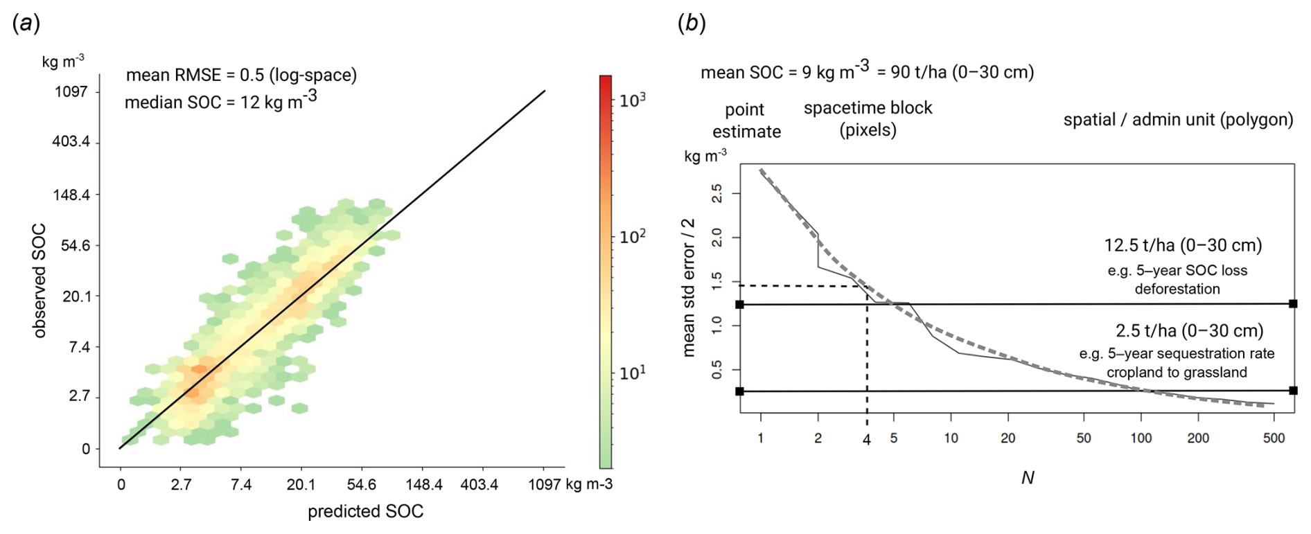
Figure 20 Simulated example of how SOC density prediction errors estimated through validation (a) relate to detection limits for different SOC sequestration/SOC loss rates (b).

From a practical point of view, most users of soil maps expect that soil predictions refer to some standard depth interval, e.g. 0–30 cm. Likewise, soil properties change gradually and often slowly; hence it is sensible to expect that, if one were to produce predictions of SOC content for every year, most of pixels in the map would not change much and this change could be significantly lower than the average prediction error. Broeg et al. (2024) showed, using revisited sites for Bavaria, that although the accuracy of the SOC prediction was high, direct validation of the derived SOC trends revealed a significantly higher uncertainty. In this work, because we also opted to generate predictions at 30 m spatial resolution, which makes this a relatively large data set, we also decided to average the values to somewhat reduce the data volumes from hundreds of terabytes to a few tens of terabytes. One could argue that we could have produced only point predictions, then let users aggregate values how ever they prefer, again we have estimated that in that case data volumes would have expanded beyond what we can handle (in terms of computing time/costs), but in the future saving the whole distributions of predictions would be an option (provided that there is enough storage for these data).

Figure 20 shows an example of the simulated effect on the standard prediction error (error of the mean) assuming averaging values of 1 to 500 points under the assumption that the SOC density follows a log-normal distribution. Assuming that the standard prediction error (RMSE) of our model is 0.5 on the logarithmic scale, and assuming that the mean value is 9 kg m⁻³ for 0–30 cm (agricultural soil), it is easy to show that the standard error of the mean for an average of 4 points (e.g. 0 and 30 cm depths and years 2000 and 2005) will be about 2.8 kg m⁻³. Following the Nyquist theorem (Hengl et al., 2013), the detection limit is RMSE$/\mathrm{2}$, hence we would be able to detect per-pixel changes which are > 1.4 kg m⁻³ per 5-year period. Assume the standard SOC sequestration rates for the conversion of cropland to grassland of approximately 0.5 t ha⁻¹ yr⁻¹ for 0–30 cm (which corresponds to ΔSOC of approximately 1.25 kg m⁻³ for a 5-year period). This means that with the model error of 0.5 on the log-scale, one would probably not be able to detect changes in SOC on a scale of 5-years, but a 20-year scale would be required (Fig. 20b). On the other hand, assuming a detection limit of 1.4 kg m⁻³, one should be able to estimate SOC loss at a time period of 5 years, assuming 2.5 t ha⁻¹ yr⁻¹ SOC loss rates for 0–30 cm depth interval, i.e., a loss of about 1.25 kg m⁻³ for 5-year intervals. If you compare with the accuracy plot for SOC density (Fig. 7) this shows that our RMSE for the SOC density on the log scale is approximately 0.5 (based on stratified sampling), which corresponds to the numbers we used above. This gives us some confidence that our predictions can at least be used to detect the serious effects of land degradation on the SOC changes, as also illustrated in Fig. 17. Broeg et al. (2024) also achieved a relatively high prediction accuracy for mapping SOC for German croplands (R²=0.61; RMSE =5.6 g kg⁻¹); however, direct validation of the derived annual SOC trends was also cumbersome (R²=0.16; p<0.0001).

Although averaging the error seems to help increase the detection limit (following the $\mathrm{1}/\sqrt{N}$ rule), we should emphasize that this does not change our average prediction error, so there is still some work to do to try to improve the prediction errors for local farms. Having shown this calculus, the RMSE of our predictions of SOCd is 0.5 on the logarithmic scale, which refers to point predictions. For block predictions, the error of the mean value is possibly about 30 %–40 % less than 0.5, so the detectable difference between two periods is possibly even more optimistic. Also note that because most of the training data come from the USA and EU (Fig. 6), it is very well possible that our prediction errors are narrower for the two continents than for the whole land mask. On the other hand, in countries where we have major gaps (Russia, Kazakhstan, China, India, tropical forests parts of Africa, and similar) we possibly perform worse than global average.

4.6 Combining global and local efforts across scales

Global predictive soil mapping efforts, such as the one described in this manuscript, overlap with local (national or regional) efforts. Is this redundancy inhibiting soil data production and confusing soil data users? Feeney et al. (2022) compared global vs local SOC predictions for Great Britain (GB) and discovered surprising inconsistencies, leading to the conclusion that we probably often underestimate the uncertainty of SOC predictions from predictive soil mapping. Users, land owners and land managers can become overwhelmed by the amount of data offered and question which to use. We instead believe that as long as some shared standards/shared open data licenses are used, local and global mapping efforts can be combined to the benefit of end users. We specifically support groups in using our global predictions as covariates in local modeling or as input for data fusion (see Fig. 21) and “federated learning” frameworks (Gallios et al., 2025). To demonstrate the synergy of local and global modeling, we are currently discussing global-local data fusion of soil carbon density predictions based on national, pan-EU (Tian et al., 2025b) and our global predictions.

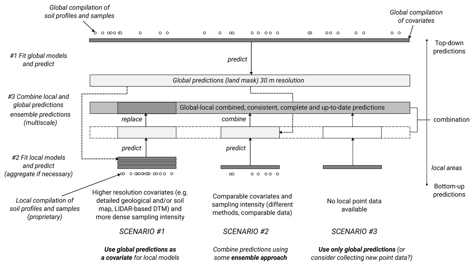
Figure 21 Proposed scheme for merging global and local soil predictive mapping outputs based on three scenarios: (1) local predictions are significantly more accurate, hence can be used to replace global predictions; (2) local and global predictions are comparable accuracy and can be best statistically combined; (3) only global predictions are available.

Although many soil mapping projects seem to overlap (as in the case of land cover mapping, for example), we believe that there is still a lot of room for multiple initiatives, as many projects are, in fact, delivering different standards. Consider the following technical specification of soil carbon in OpenLandMap-soildb (one of the Essential Climate Variables of the Global Climate Observing System):

• Referent variable: soil organic carbon density in kg m⁻³;

• Referent laboratory method: DC ISO 10694:1995(E);

• Measurement support size: 1×1 m horizontal, 5 cm vertical;

• Prediction depth interval: 0–30 cm;

• Prediction time-interval: 2000–2005;

• Prediction error distribution: 68 % probability (1 standard deviation);

In order to combine the predictions of two projects as shown in Fig. 21, both local and global should match in all specifications; otherwise, differences in values could be unrelated to the accuracy of each individual map. A “soil carbon map” tag is no longer specific enough. We probably need to start using more specific standards and specifications where soil variables match at least in reference laboratory methods, measurement units, and temporal coverage – for example, “5-year soil carbon stocks for 0–30 cm depth interval for 2000–2005”. Products from different projects could possibly be harmonized, but in general, without complying with the same standard, it is probably not necessary to compare or criticize what are essentially different soil data products; for example, the predictions of the organic carbon content of soil (%) are not 1:1 with the predictions of soil organic carbon density (kg m⁻³), which is also illustrated in Figs. 2a and 18b.

4.7 Broader impacts and possible future development directions

In 2008, a group of world leaders in digital soil mapping launched the idea of mapping soils for the entire world at a high spatial resolution of 100 m: the GlobalSoilMap.net project (Hempel et al., 2014). The main idea of GlobalSoilMap was to produce global maps in a resolution compatible with publicly available SRTM DEM (90 m), at that time one of the most popular global environmental products. In the original plan, the proposal was to achieve this per country, then to combine all data together. Although stitching high-resolution national soil maps to produce global data sets is technically possible and politically correct (see, e.g. FAO, 2022), it has been shown to lead to significant differences at political borders. In addition, often a large number of countries are left blank, leading to limited usability of such data.

In 2009, it seemed that GlobalSoilMap could be achieved in a few years time, but this was a gross underestimate. It took almost 18 years to produce complete and consistent soil property maps with comparable spatial resolution. Thanks to the exponential development of computing and Machine Learning, we are now able to predict not only soil properties at 100 m, but at 10× finer volumes and in space-time. However, this long delay in producing soil data that matches most land cover and vegetation products indicates that global soil mapping is complex, especially with soils being hidden, buried, and impacted by multiple soil-forming processes working at the same time in a non-linear way (compared to vegetation and land cover mapping where EO images often suffice), having high short-range variability, and often based on unrecorded historic processes including extreme events such as flooding, landslides, vertical movement of materials, and similar. The mapping of soils remains one of the most challenging tasks in physical geography.

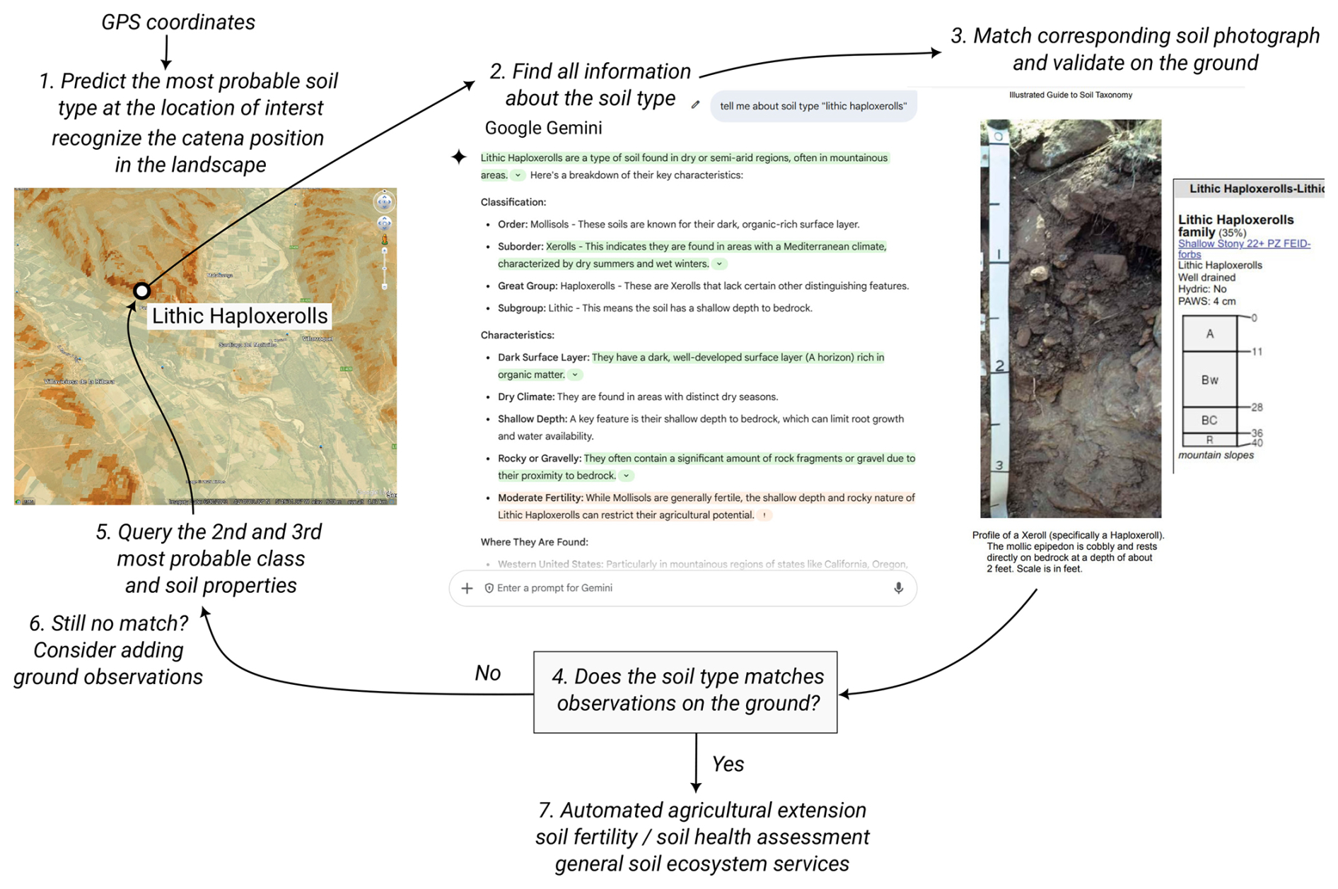
Figure 22 Example of how LLM's (in this case Google's Gemini™) can be directly combined with the global data sets we have produced to help with understanding the soils better and with taking actions. Image and text source: USDA's Illustrated Guide to Soil Taxonomy.

We foresee the following future development directions in dynamic soil mapping (unsorted):

• Hybrid Machine-Learning/Process-Based modeling: there is increasing interest in the so-called “Knowledge-based ML”. Liu et al. (2024) shows how a relatively detailed model ecosys can be combined with ground measurements to recalibrate modeling and optimize accuracy. The ecosys framework requires a large number of inputs, produces daily values, and is currently optimized for agricultural systems. The computational load required to run ecosys at 30 m for all land mask would be enormous. In the meantime, we recommend to all soil mappers to at least put effort to develop ML models following “Soil Science-Informed ML” e.g. by specifying observational priors, pseudo-observations, adding model structure designs and loss functions (Minasny et al., 2024).

• Global digital soil twin: assuming that we manage to integrate state-of-the-art process-based models with high resolution EO data and in-situ laboratory measurements, one could expect that one day we will be able to model soil-vegetation-land-use-climate interactions within a paradigm of digital soil twin (digital copy of the world soils is connected with the physical twin and data automatically flows in two directions).

• Development of rapid and cost-effective in-situ soil sampling instruments: soil laboratory analysis remains costly and global training data sets are often limited to most developed nations. Modern in situ technologies such as soil spectroscopy and similar show that the costs of measuring soil chemical and physical soil properties can be reduced to fractions of traditional soil laboratory costs (e.g. about USD 150 per sample). In addition, land owners often do not have patience to wait weeks until the results of laboratory analysis are released. Here, one of the most striking examples is the LUCAS soil survey, where soil laboratory data takes almost 3–5 years until they are released. Some recent results with relatively cost-effective NIR instruments show that there is an opportunity to use a handheld near-infrared device (NIR, 1350–2550 nm) for near-real-time SOC measurements (Kalopesa et al., 2025). The results of using the YardStick™ instrument (Gyawali et al., 2025) also show satisfactory results with the opportunity to scan changes in soil properties every 1 cm of depth (continuous functions).

• Finer-temporal resolution modeling: in this paper we mapped soil properties using annual values of bio-physical indices and climatic variables. Many soil variables could also be mapped at bimonthly or monthly temporal resolutions. For example, many geochemical soil properties, such as available Nitrogen (N), Phosphorus (P), and Potassium (K), have been shown to vary within a few weeks between sampling; soil moisture is even more variable, with values changing within hours. Again, to map the world at monthly intervals at high spatial resolution would be extra computationally intensive and is certainly beyond our state of technology. However, we have recently produced bimonthly 30 m resolution GPP (Isik et al., 2025), so this is definitely possible, but we would likely have to limit any such models to top-soil only and 1–2 soil variables.

• Using multi-response models to model and predict all variables using a single model: In this work, we fit multiple separate models for each property. This means that we assume that all target variables are independent, but they are not. To deal with multi-colinearity and overlap in target variables, one could fit a very holistic single model able to predict multiple depths and soil properties all at once. This multi-output approach works better for values that are somehow correlated and is also more elegant as the prediction would be for all properties at once. Random Forest is again applicable statistical method here, as it supports multi-response models and predictions.

• Using global Generative Foundation Models: currently there is increasing interest in building global foundation models or World Foundation Models (WFMs) that would basically include all literature on soils (tabular, textual data, schemes, and scientific visualizations) and would be able to represent world soil distribution and properties. Bodnar et al. (2025) recently released “Aurora”, a large-scale foundation model trained on more than one million hours of diverse geophysical data, and which can outperform several existing weather forecasting operational systems while also being orders of magnitude faster. Once such models become robust and convincing, they could be used to connect users directly with the data, which could make many traditional soil scientists and agronomists redundant. An example of how LLMs can already be used to boost knowledge about soils is shown in Fig. 22.

• Hyperspectral EO missions: Although spatiotemporal models can be relatively accurate with a high R², the detected changes based on EO predictions are often of limited use: EO-derived SOC estimates have a low signal-to-noise ratio, and hence the detection of precise SOC changes over time remains cumbersome. Harris and Bardgett (2025) recently tested using hyperspectral (drone-based) images and got promising results even for mapping soil microbial community composition. In that sense, ESA's Copernicus Hyperspectral Imaging Mission for the Environment (CHIME) and NASA's Surface Biology and Geology (both planned to launch in 2028) might offer an unprecedented opportunity to map soil variables at high spatial resolution. However, hyperspectral imaging might not become a “silver bullet” for all soil variables.

On the one hand, we can anticipate many exciting developments in soil science in the near future; on the other hand, we recognize that soil science seems to be actively diverse, lagging behind many other environmental fields, especially in terms of having stable cyberinfrastructures and standards. For example, when it comes to soil laboratory data, there are now at least five independent initiatives where global soil point data have been prepared and made ready for modeling:

1. WoSIS soil profiles and samples (Batjes et al., 2024);

2. International Soil Carbon Network (ISCN) (Harden et al., 2018);

3. Open Soil Spectral Library (OSSL) (Safanelli et al., 2025);

4. SoDaH: SOils DAta Harmonization database (Wieder et al., 2021);

5. SoilHive (https://www.soilhive.ag/, last access: 6 June 2025) hosted by the Varda foundation shows all soil data available for any location in the world (both point, polygon, and raster layers);

Compare this with databases produced in the fields of biodiversity, biology, meteorology, or similar:

1. GBIF (the Global Biodiversity Information Facility; https://www.gbif.org, last access: 6 June 2025) with 3 billion occurrence records;

2. NOAA's hosted GHCN (Global Historical Climatology Network) with over 100 000 meteorological stations and 1B of daily measurements;

3. FLUXNet (https://fluxnet.org/data/, last access: 6 June 2025) with hourly measurements of some 100+ biophysical variables at more than 250 automated measurement stations worldwide;

4. GLANCE (https://doi.org/10.34911/rdnt.x4xfh3, Stanimirova et al., 2023b) with more than 2M observations of land cover;

5. GEOROC Database (Geochemistry of Rocks of the Oceans and Continents; https://georoc.eu/georoc/, last access: 6 June 2025) containing almost 30M values of major and trace element concentrations, radiogenic and nonradiogenic isotope ratios, etc;

It is easy to notice that soil science is seriously lagging behind GBIF and similar initiatives. In our opinion, global soil science critically misses: (a) a global (permanent) soil monitoring network of at least 300–500 permanent stations where soil properties can be tracked on a monthly/annual basis, (b) professional infrastructure where various groups can enter and access point data (compare to https://www.gbif.org/dataset/, last access: 6 June 2025), and (c) agreements on data sharing, soil sampling (Even et al., 2025), and open soil laboratory standards including a universal soil classification system blessed by the IUSS (International Union of Soil Science).

An inspiring model for monitoring soil properties over time is the International Soil Moisture Network (https://ismn.earth/, last access: 6 June 2025) that provides open access to approximately 3200 automated measurement stations with hourly measurements of soil moisture, temperature, precipitation, and similar (Dorigo et al., 2021). Another infrastructure critically missing in soil science, in our opinion, are globally applicable mobile phone apps that allow anyone to take photographs of soil, soil spectral scans, and similar and share (as in, e.g. iNaturalist app). Many soil enthusiasts and agronomists have asked us in the past “How do I share my data?”. At the moment, we can only recommend to those colleagues who register their (in situ) data on https://Zenodo.org, last access: 6 June 2025, https://SoilHive.ag, last access: 6 June 2025 or similar, obtain a DOI and then let us know that we can import and integrate your data into these models to help build better soil maps for everyone. The LandPKS app (https://landpotential.org/mobile-app/, last access: 6 June 2025) could here potentially play an important role if it extends its functionality to soil laboratory data, soil profile photographs, and soil spectral scans.

Aroca-Fernandez et al. (2025) recently developed a framework called WALGREEN, which runs on top of Google Earth Engine and the Copernicus Data Space Ecosystem, and shows how to generate SOC predictions on-demand (that is: select an area of interest, drop training points, and download SOC predictions). WALGREEN is primarily based on EO images, and the performance in terms of accuracy and robustness is currently unknown. Automation of modeling, predictions, even automated deployment of maps in an app is a reality today. However, knowledge of soil science is needed more than ever. The application of all these (AI) tools has become much easier, so we have to spend much less time in actually implementing machine learning and statistics, but at the same time we still need to know what we do and have a clear picture of what to put the outcome into perspective, to actually be able to have a proper interpretation of the outcome and the results; and without a sufficient background knowledge we will not be able to put it into perspective.

5 Data availability

The data products produced can be accessed via the associated repository records (Consoli et al., 2025, https://doi.org/10.5281/zenodo.15470431; OpenGeoHub Foundation, 2026, https://world.soils.app/), while the training dataset is available via Hengl and Gupta (2025, https://doi.org/10.5281/zenodo.4748499). Due to Zenodo's storage limitations and the large size of the dataset, only portions of the data are stored in Zenodo, distributed across multiple buckets. We provide predictions of soil properties in 120 m resolution with uncertainty (16th percentile, mean, and 84th percentile) for only the first and last period (2000–2005 and 2020–2022+). In addition, we provide soil type probability maps in 120 m resolution based on USDA Soil Taxonomy, organized at the subgroup level. Complete global 30 m resolution mosaics are available through the Google Earth Engine (https://code.earthengine.google.com/?asset=projects/global-pasture-watch/assets/gsm-30m, Hengl et al., 2026).

Each data set layer follows a standardized naming format, structured into 10 key fields: generic variable name, variable procedure combination, position in the probability distribution or variable type, spatial support, depth reference, time reference (including start and end times), bounding box, EPSG code, and version code. Each metadata field serves a specific purpose in assessing the datasets' fitness for use. For the data sets presented in this study, the metadata specify a uniform spatial support of 30 m resolution, a depth reference denoted as s (depth from the surface), a bounding box identified as go, and an EPSG code of EPSG:4326. For the other fields: the generic variable name helps users identify the required predictor layer; the variable procedure combination provides indications of how the data were derived and its source; the time reference, comprising the start and end dates, ensures users can select layers matching their relevant temporal scope; and the version code, which reflects the creation date of the corresponding layer, facilitates tracking and version control.

6 Code availability

The code used to harmonize the training points and generate predictions is available under the MIT license at https://doi.org/10.5281/zenodo.15608971 (Hengl et al., 2025).

7 Conclusions

We have produced the first batch of 30 m resolution soil property annual dynamic maps for 2000–2022+. This is an open data output aiming at serving international modeling and monitoring projects, especially the UNCCD's Land Degradation Neutrality programme, FAO's Global Soil Partnership and similar, to help countries and land owners get baselines of their soil stocks and better understand the soil dynamics. For modeling, we use state-of-the-art harmonized soil laboratory data sets (training points) that we have been collecting and improving over the years. We make import procedures transparent and fully documented via https://soildb.OpenLandMap.org/. The results indicate that (research question #1) Landsat-derived biophysical indices rank high in the variable importance results, especially with GPP coming in the top three most important variables and showing a clear positive correlation with SOC density. These results indicate clear interconnection between GPP and SOC accumulation, and a warning to all land use systems that decrease annual GPP – this will likely also result in significant losses in SOC. The prediction accuracy assessment indicates that (research question #2) the best achievable mapping accuracy is RMSE of 17.7 [kg m⁻³] (0.486 in log-scale) for SOC density, RMSE of 51.3 [g kg⁻¹] (0.574 in log-scale) for SOC content, RMSE of 0.15 [t m⁻³] for bulk density of fine-earth, RMSE of 0.51 for soil pH, RMSE of 8.4 % for soil clay content, and RMSE of 12.6 % for soil sand content, respectively. Further analysis of trends in SOC density and soil pH indicates that (research question #3) the key drivers of negative changes in SOC are land degradation, primarily the conversion of tropical forests to cash crops; for soil pH, the most important explanatory variable appears to be the CHELSA Aridity Index (long-term), annual precipitation, and salinity grade. Finally, (research question #4) the remaining hot spots of global SOC are boreal peatlands (of Canada and Russia) and tropical peatlands storing the majority of total soil carbon. Especially Canada and the Russian Federation seem to contain most of the world's soil carbon. We estimate that the world has lost at least 11 Pg of SOC in the top soil in the period 2000–2022+ and that the current SOC stock of the land is 461 Pg for 0–30 cm.

The 30 m resolution predictions of soil properties and USDA subgroups show an unprecedented level of detail; however, we warn users that prediction errors are still relatively wide and that this uncertainty (per pixel) should be incorporated into decision making to prevent taking high-risk decisions. Further recommended uses of these data include: continental soil carbon dynamics monitoring, derivation of secondary soil variables such as soil hydraulic properties using pedotransfer functions, land degradation, and soil health assessment.

We plan to update these predictions for each subsequent year and also as the new point data sets become available. We currently engage in Data-Sharing Agreements for various soil datasets that are not in the public domain, and we would like to engage with more countries outside of Europe in a similar manner. In addition, for those countries which consider accurate position of sample locations (GPS coordinates) to be private data, we would like to extend this to the federated model space, which would further enable global products to be aligned with (finer resolution) national products becoming available in a few jurisdictions. Additional improvements in the accuracy of the dynamic predictions can be implemented by combining global and local models, especially at national scales. The only requirement for further data fusion is that all parties use the same standard (e.g. 0–30 cm; 5-year time blocks; DC reference laboratory methods and similar). We call on research groups to use these data to derive secondary soil properties and test their applicability for real-world applications.