the Creative Commons Attribution 4.0 License.
the Creative Commons Attribution 4.0 License.
 | 20 Nov 2026
SMHIGridClim, 2.5 km resolution gridded climatology of Fennoscandia
Sandra Andersson

Maria Norman
Tomas Landelius
Patrick Samuelsson
Semjon Schimanke
Maida Zahid
Lars Bärring
SMHIGridClim, the Swedish Meteorological and Hydrological Institute Gridded Climatology, covers Fennoscandia at 2.5 km horizontal grid resolution for the period 1961–2018. It includes 2 m temperature and two-metre relative humidity at 1, 3, or 6 h temporal resolution (which varies over the covered period), as well as daily minimum and maximum temperatures, daily precipitation, and daily snow depth. The gridding is performed using optimal interpolation with the open-source software gridpp from the Norwegian Meteorological Institute. Observations used in the analysis are provided by the Swedish, Finnish, and Norwegian meteorological institutes, as well as the European Centre for Medium-Range Weather Forecasts (ECMWF). Quality control of the observations is conducted using the open-source software TITAN, also developed at the Norwegian Meteorological Institute. The first guess for the optimal interpolation is obtained from the UERRA-HARMONIE reanalysis at 11 km horizontal grid resolution, which is statistically downscaled to fit a subset of the operational ensemble numerical prediction system at 2.5 km horizontal grid resolution, with daily and yearly variations in the downscaling parameters. The quality of the analysis varies over time and depends on both the accuracy of forecasts and the quality and density of available observations. In terms of annual mean root mean square error (RMSE), the quality of SMHIGridClim is comparable to similar gridded datasets covering the Nordic countries. SMHIGridClim is available at https://doi.org/10.7910/DVN/ZFZL6K (Andersson et al., 2025).
- Article
(15618 KB) - Full-text XML
- BibTeX
- EndNote


Gridded climate datasets with high resolution and long-term coverage have become vital for climatological and environmental research (Brohan et al., 2006; Aalto et al., 2016; IPCC, 2021). These datasets enable researchers to assess climate change and its impacts, providing valuable insights for formulating sustainable approaches to climate challenges (Overpeck et al., 2011). Compared to point data, gridded datasets offer several advantages as they are generally user-friendly, offer mostly uniform spatial coverage, ensure consistent temporal coverage and seldom have missing data (Essou et al., 2016). Even so, they have their drawbacks (e.g., real-time availability and potential inaccuracies in regions with sparse observation networks) that make them inadequate for many applications in regions with complex topography (Zandler et al., 2019; Mankin et al., 2025). Moreover, gridded datasets often lack consistency between variables. The exception is reanalysis datasets which are based on dynamical models.
Northern regions, particularly the Arctic areas are at the forefront of climate change discussions due to their rapid warming (IPCC, 2013; Fountain et al., 2012). The climate change signal is also quite noticeable across Fennoscandia (Finland, Sweden and Norway), with altered hydrological cycles, rising temperatures, changing ecosystems, and increasing challenges for infrastructure, agriculture, and water resource management (Førland et al., 2002; SOU, 2007; Tietäväinen et al., 2010; Nikulin et al., 2011; Mikkonen et al., 2015; Grusson et al., 2021; Lind et al., 2023). However, addressing these issues requires localised, reliable, and high-resolution climate datasets that can capture both regional variations and local-scale climate features well.
Traditional global climate models (GCMs), while valuable, fail to offer the level of detail needed for regional or local-scale assessments. To fill this gap, various well-recognised gridded datasets such as the Climate Research Unit (CRU) dataset (Harris et al., 2020), the E-OBS database (Haylock et al., 2008; Cornes et al., 2018), the European Climate Assessment and Dataset (ECA&D) (Klein Tank et al., 2002; Klok and Klein Tank, 2009), the Global Precipitation Climatology Centre (GPCC) dataset (Yu et al., 2020), the HadGHCND dataset (Caesar et al., 2006), ERA Interim (Dee et al., 2011), the ERA5 dataset (Hersbach et al., 2020), and CERRA (Schimanke et al., 2021) are widely available online and frequently used for climate impact assessment, climate adaptation and mitigation purposes. Each of these datasets has its strengths and limitations, and understanding these distinctions is crucial for selecting the most appropriate data for specific climate studies.
Among the climate datasets for the Nordic region, the Nordic Gridded Climate Dataset (NGCD) from Met Norway (Lussana et al., 2018, 2019) has emerged as a strong candidate for climate analysis. The NGCD covers Fennoscandia (Finland, Sweden, and Norway) at a horizontal grid resolution of 1 km, with data available from 1961 to the present. The dataset contains daily air temperature (mean, maximum, and minimum) and daily precipitation. There are two main constraints of this dataset: (1) it does not provide sub-daily information for the variables, and (2) the input data used to produce NGCD has low coverage of stations, which may result in uncertainties, particularly in remote northern regions (Tveito and Lussana, 2018). Another potential candidate is data from the UERRA surface reanalysis, MESCAN-SURFEX (Soci et al., 2016; Bazile et al., 2017; Le Moigne et al., 2020). The spatial resolution of the MESCAN-SURFEX data is 5.5 km, with a time span from 1961 to 2018. This dataset provides analysis of daily accumulated precipitation and six-hourly analyses of air temperature, wind, and relative humidity, but it lacks maximum and minimum temperature data. Furthermore, MESCAN-SURFEX has shown some quality issues with precipitation (Soci et al., 2016; Monteiro and Morin, 2023).
To address the discrepancies in existing gridded datasets for the Nordic regions, a high-resolution dataset called SMHIGridClim (Swedish Meteorological and Hydrological Institute Gridded Climatology) has been developed. The primary aim of this dataset is to provide high-quality, long-term climate information for Sweden. Additionally, it offers comprehensive climate data for regional analysis across neighbouring countries like Finland and Norway. In this paper, a detailed overview of the SMHIGridClim dataset is provided to assist users in understanding its structure, features, variables, and potential applications for climate analysis in the Nordic regions.
SMHIGridClim is developed to meet the need for a climate reference dataset that offers high temporal resolution (sub-daily), fine spatial resolution (2.5 km horizontally), a long-time span (starting from 1961), key climate indicators (see below), and spatial coverage across Fennoscandia and the Baltic States. Above all, SMHIGridClim is specifically designed for use in climate scenario services. It offers a reliable source of historical climate data, enabling researchers to investigate past climate conditions with greater precision and accuracy. Moreover, the dataset can be used to adjust the output of climate models to correct biases. In short, SMHIGridClim represents valuable data applicable across various sectors, including agriculture, forestry, hydrology, and urban planning, to improve climate-related decision-making at regional scales. The dataset has, for instance, been used in research connecting people's health with the weather (Raza et al., 2024).
The methodology behind SMHIGridClim is based on optimal interpolation, combining ground-based observations with gridded forecasts (the initial state of the variables) originating from downscaled fields from UERRA-HARMONIE. The downscaling, from originally 11 km horizontal grid resolution to 2.5 km horizontal grid resolution, was done based on linear regression with daily and yearly variations in the downscaling parameters, using the operational ensemble numerical prediction system at SMHI. The dataset covers Fennoscandia and the Baltic States during the time period 1961–2018 and includes the variables 2 m temperature (tas) and relative humidity (hurs) with 1-, 3-, and 6-hourly resolution (depending on the time period), along with daily precipitation (pr), snow depth (snd), maximum (tasmax), and minimum (tasmin) temperature.
The structure of the paper is as follows. Section 2 presents the data included in the analysis, along with the tool for quality control. Section 3 describes the analysis method and provides an overview of the gridpp performance. Section 4 presents the results from the validation of SMHIGridClim, which are further discussed in Sect. 6, together with the conclusions. Data availability is presented in Sect. 4 while author contributions and acknowledgements are given in Sects. 7 and 8 respectively.
The data used in the analysis consist of in-situ observations and gridded fields from numerical weather prediction (NWP) models. Figure 1 provides an overview of the processing steps and the variables included in SMHIGridClim. For near-surface humidity, the analysis is based on dew point temperature at 2 m (tdps) rather than relative humidity. This choice is motivated by the difficulty of analysing a variable with hard physical bounds, as is the case with relative humidity. Additionally, snow depth is not available from the UERRA-HARMONIE dataset and was therefore derived from snow water equivalent and snow density.
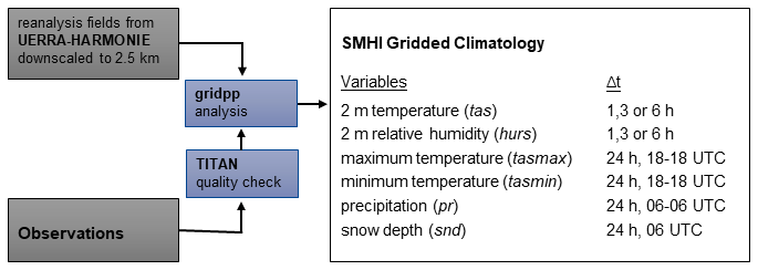
Figure 1Overview of the processing steps of data for analysis with gridpp, and the produced variables in SMHIGridClim.
2.1 Observations
2.1.1 Observational data sets
Local in-situ observations were collected from the national meteorological institutes in Sweden, Norway and Finland, as well as from ECMWF's MARS archive. The Swedish observations were extracted from SMHI's Meteorological Observational Real-time Archive (MORA) database. Since SMHI has an open data policy, the data are freely available, and more information (in Swedish) can be found at: https://www.smhi.se/data/ (last access: 11 June 2026). Historical data from the Norwegian Meteorological Institute, also freely available, were retrieved using their Frost API: https://frost.met.no (last access: 11 June 2026). Data from Finland were obtained from the Finnish Meteorological Institute's internal database, also freely available: https://en.ilmatieteenlaitos.fi/open-data (last access: 11 June 2026).
During the early years of the SMHIGridClim period, only a few tdps observations were available in the Norwegian national data. Therefore, tdps was derived from tas and hurs using gridpp.dewpoint function from the gridpp library, which calculates the dew point temperature by inverting the Magnus–Tetens approximation formula relating saturation vapor pressure to temperature:
where the unit for both tas and tdps is in degrees Celsius.
For all data streams, tdps was checked to ensure it did not exceed the observed tas. If a tdps value was higher than the corresponding tas + 5 °C, it was set to missing. If it was between tas and tas + 5 °C, it was adjusted to match tas.
In addition to observational data from the national archives, all relevant surface data, specifically SYNOP station observations stored in BUFR (Binary Universal Form for the Representation of meteorological data) format (WMO, 2025), were retrieved from the ECMWF's MARS archive. Variables extracted include tas, tdps and snd.
2.1.2 Observation density
Observation density varies over both decadal and diurnal time scales, and it also differs depending on the observed variable.
Figure 2 shows examples of the spatial distribution of observations for tas, tasmax/tasmin, pr, and snd during a month in 1965. In the early years of the SMHIGridClim period, ECMWF BUFR data were limited for tas and snd, making the national datasets particularly important. For observations of tasmin, tasmax, and pr, the national data are crucial, as BUFR data are not available at all during this early period. Across all datasets, the northern part of Scandinavia shows areas with sparse data coverage – notably in northern Sweden near the Norwegian border, and in northern Finland near the Swedish border. These areas of relatively low observation density are associated with higher uncertainty in the analysis.
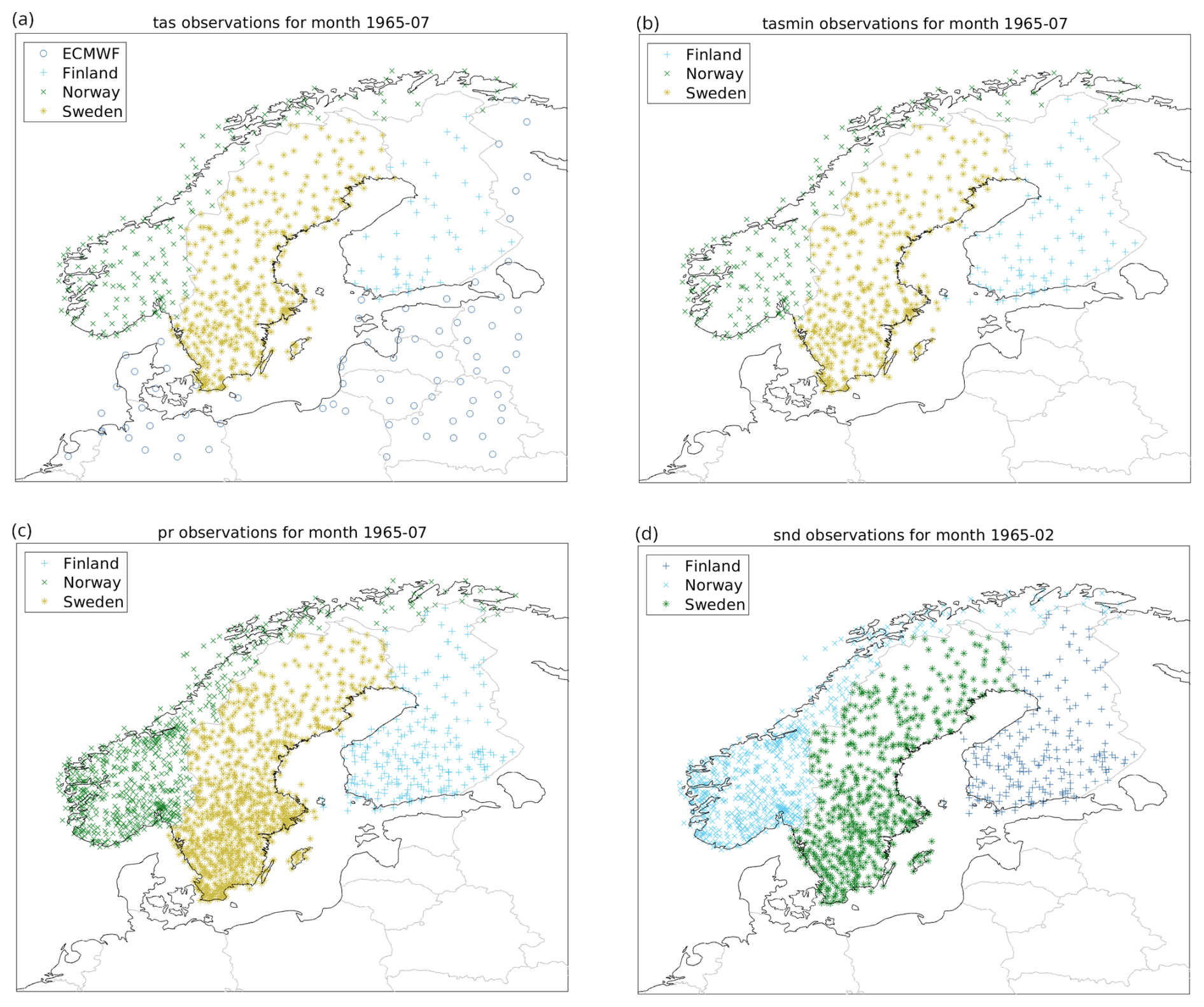
Figure 2Observation density maps of (a) tas, (b) tasmin, (c) pr and (d) snd. Maps include data since July 1965 (February for snd) from different data sources indicated in the legend. Observations represent those that are available for the whole month.
Figure 3 shows observation density on a decadal scale. There is a marked increase in the number of tas observations from 1995 onwards. This is primarily due to the expansion of automatic weather stations, which report at higher frequency – typically hourly. The increase in the number of tasmin observations reflects only the densification of the station network, as this variable is reported once per day. For all data streams, the number of pr observations has declined from the 1980s onwards. The number of snd observations shows no clear trend for Swedish and Finnish data, while the Norwegian station density shows a distinct decline between 2000 and 2005.
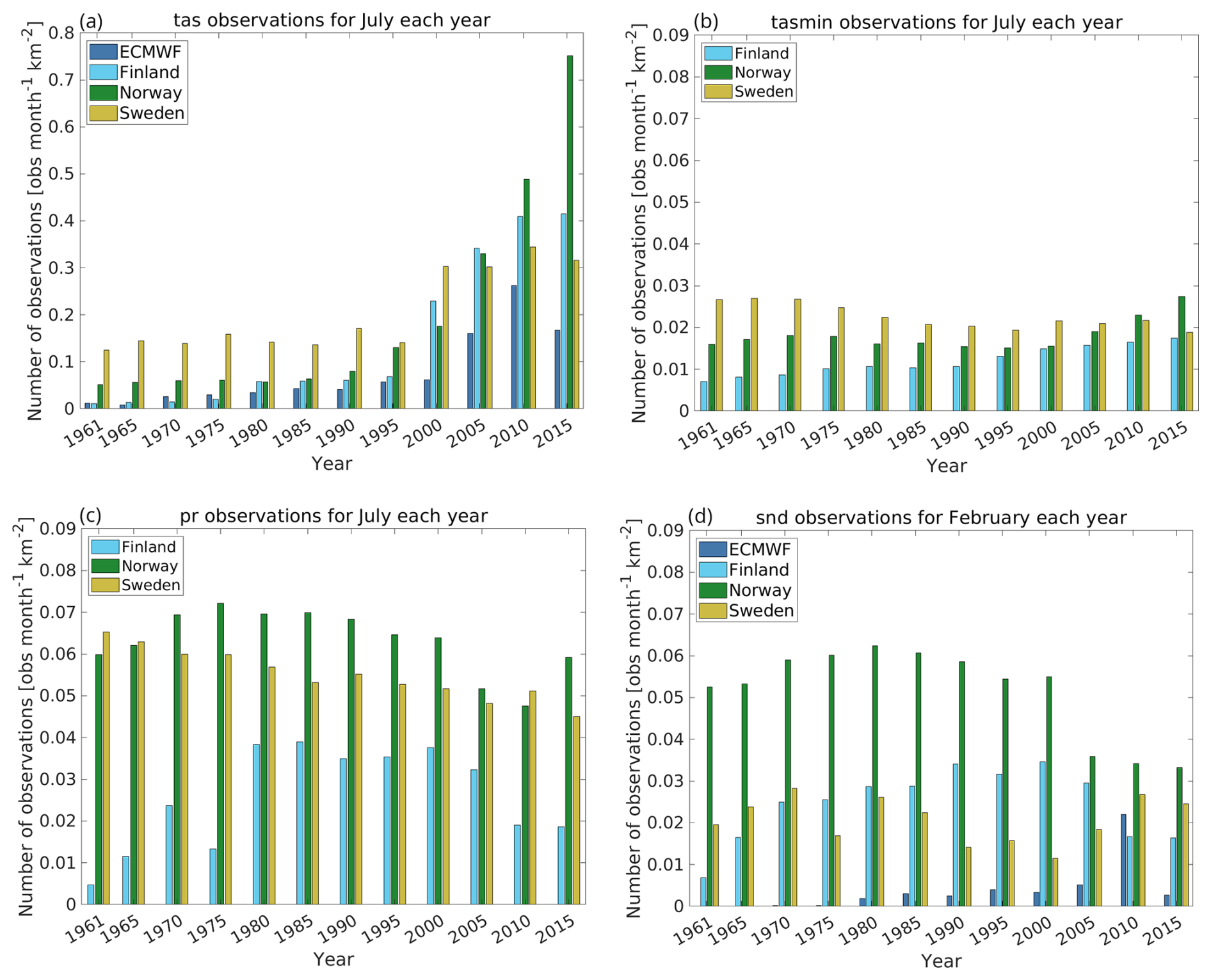
Figure 3Observation density bar plots per year for (a) tas (July), (b) tasmin (July), (c) pr (July) and (d) snd (February). The bars are colour coded with respect to data sources as indicated in the legends. The observations represent those that are available for the whole month taken into account that they are considered valid within specified limits.
The number of tas and tdps observations during the day varies over time, as a consequence of observation frequency and the amount of digitalised data. A preliminary analysis showed that it is not meaningful to analyse more than every 6th hour for the period 1961–1967, and every 3rd hour for the period 1968–1996. From 1997 and onward the network (mainly due to the introduction of the automatic stations) provides enough observations to allow an analysis for every hour of the day. However, the density of observations still varies considerably between the traditionally reporting hours (06:00, 12:00 and 18:00 UTC) and the intermediate ones.
2.2 Observation quality control
Observation quality control was carried out using the TITAN package (https://github.com/metno/TITAN/wiki, last access: 27 August 2026), developed at Met Norway (Båserud et al., 2020). Note that TITAN has been replaced by a new package, titanlib (https://github.com/metno/titanlib/wiki, last access: 27 August 2026).
TITAN requires input data including station coordinates (latitude and longitude), station altitude, and the observation to be checked. All observations are assumed to be independent in time, as TITAN does not account for temporal correlations. The package offers several quality controls (QC) tests and configuration options (Båserud et al., 2020). The specific checks used in this study are summarised in Table 1. For further details on the TITAN settings, we refer to Andersson et al. (2021).
Table 1The table presents the TITAN quality checks together with a short description. Options used in the present study, and the DQC number, where it is applicable, is also shown. Refer to Andersson et al. (2021) for full documentation of TITAN settings.
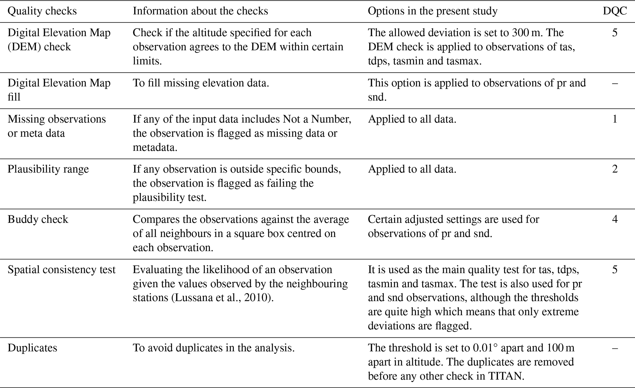
The TITAN outputs a Data Quality Control (DQC) code that indicates whether the observation is considered valid (DQC = 0) or suspicious (DQC > 0). Note that the isolated station check in TITAN was disabled in this study.
In addition to the checks performed by TITAN, a gross error check was applied using the first guess from the analysis. The first guess was interpolated to the observation locations using bilinear interpolation. For temperature variables, the interpolation accounted for elevation differences between the model grid and the station location, using lapse rates of −0.0065 K m−1 for tas and −0.0017 K m−1 for tdps. Fixed lapse rates may be unrepresentative during temperature inversions or other conditions with anomalous vertical temperature gradients. Because the elevation correction is applied before the gross-error check, this could occasionally cause valid observations to be rejected, particularly where station and grid elevations differ substantially. The three-standard-deviation threshold limits, but does not eliminate, this risk; future versions could instead use dynamically estimated lapse rates or model-derived vertical gradients.
If the difference between the observation and the interpolated first guess exceeded three times the standard deviation of all differences, the observation was considered a gross error and was removed.
This gross error check was applied to all variables except for daily precipitation (pr), as precipitation fields can be highly variable and spatially discontinuous. Applying the check to pr could lead to the erroneous removal of valid but spatially patchy observations (e.g., local showers not captured by the forecast model).
2.3 Numerical weather prediction data
Forecasts from the UERRA-HARMONIE reanalysis (Copernicus Climate Change Service, Climate Data Store, 2019) were used as the basis for creating the first-guess fields in the SMHIGridClim analysis. Importantly, the analysis fields from UERRA-HARMONIE (available at 00:00, 06:00, 12:00, and 18:00 UTC) were not used as first guesses, as they include information from some of the observations included in the analysis.
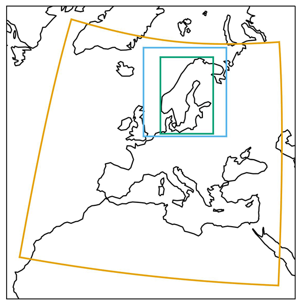
For an overlapping time period (January 2016 to July 2019), the UERRA-HARMONIE fields were complemented with corresponding forecasts from the Nordic operational NWP system MEPS (Meteorological Ensemble Prediction System, Frogner et al., 2019). These forecasts, together with the UERRA-HARMONIE data (with a horizontal grid resolution of 11 km), were downscaled to the SMHIGridClim domain. The SMHIGridClim grid is defined as a subset of 823×567 points from the MEPS grid, with a horizontal grid resolution of 2.5 km. The spatial coverage of UERRA-HARMONIE, MEPS, and SMHIGridClim is shown in Fig. 4. The downscaling process is described in detail in Sect. 3.1.
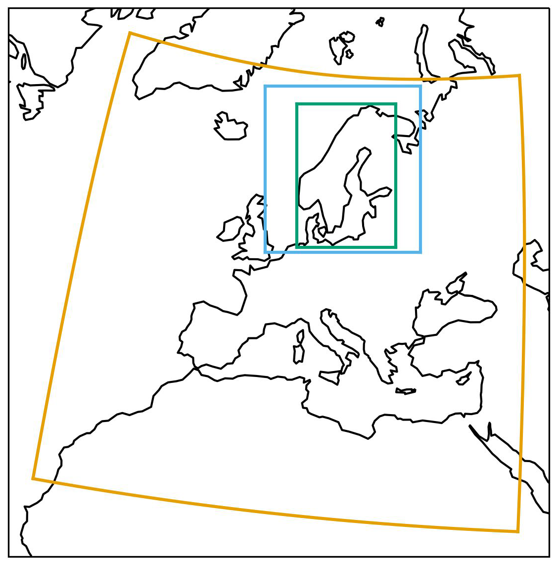
Figure 4The areas covered by the different model grids of datasets in this paper. Orange: UERRA-HARMONIE at 11 km. Blue: MEPS at 2.5 km. Green: SMHIGridClim at 2.5 km (subset of the MEPS grid).
Table 2 provides an overview of the forecast cycles and lead times used for each variable in the SMHIGridClim dataset. For tas and tdps, MEPS data were retrieved as 6 h forecasts: 00+06, 06+06, 12+06, and 18+06. No direct MEPS fields were available for tasmin or tasmax. Instead, relationships based on tas at midpoints of the tasmin and tasmax time windows were used, as shown in Table 2. Precipitation (pr) was derived from a combination of accumulation periods, while snow depth (snd) was assumed to be measured at 06:00 UTC and was therefore based on the 00+06 forecast. However, snd is not available as a model output from either UERRA-HARMONIE or MEPS and was derived from snow water equivalent and snow density. Since snow density is not available from MEPS, only snow water equivalent was downscaled from UERRA-HARMONIE. This derivation is further described in Sect. 3.1.
Table 2Forecast cycles and lengths of the UERRA-HARMONIE fields for the different entities in the SMHIGridClim data set (SWE is snow water equivalent, and rho is snow density).
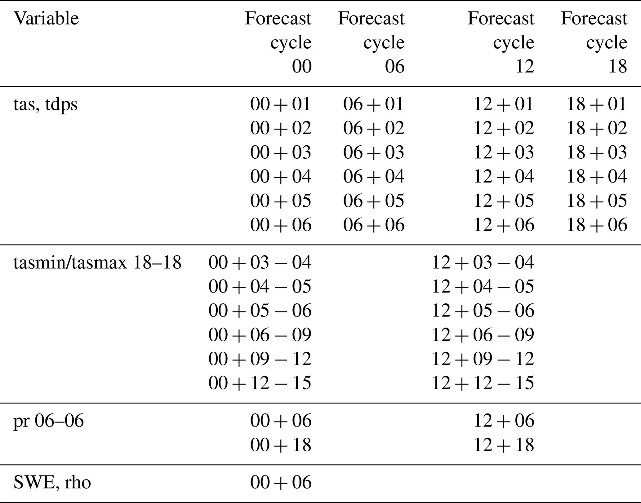
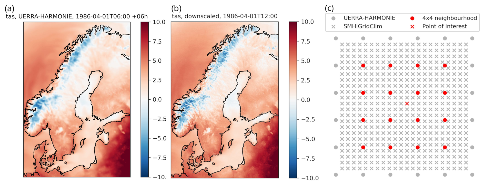
Figure 5Example illustrating the downscaling of temperature from UERRA-HARMONIE to the 2.5 km grid used in SMHIGridClim. (a) Original UERRA-HARMONIE field interpolated to the SMHIGridClim grid (unit: degrees Celsius). (b) Downscaled field. (c) Schematic illustration of how a point (red cross) in the 2.5 km grid is associated with its 4×4 neighbourhood (red dots) in the 11 km UERRA-HARMONIE grid.
3.1 Downscaling the first guess
Data from the overlapping MEPS and UERRA-HARMONIE period (see Sect. 2.3) were used to establish a relationship based on linear least squares regression. The regression was performed between a given point on the SMHIGridClim domain (2.5 km horizontal grid resolution, derived from the MEPS grid) and its surrounding 16 nearest neighbouring points in the UERRA-HARMONIE grid (11 km resolution).
Figure 5 shows an example of tas from UERRA-HARMONIE interpolated to the 2.5 km grid and the corresponding downscaled fields. The downscaled tas demonstrates finer spatial structure, particularly in mountainous regions of Norway and Sweden. The right-hand panel of Fig. 5 illustrates how each grid point in the 2.5 km grid is linked to its 16 nearest neighbours in the 11 km UERRA-HARMONIE grid.
For tas and tdps, four separate weighted regressions were calculated – for day and night (00:00 and 12:00 UTC), and for mid-winter and mid-summer, respectively. Final weights, combining diurnal and seasonal variation, were computed using squared cosine functions centred at 00:00 and 12:00 UTC, and at day numbers 0 and 183. The weighting functions are illustrated in Fig. 6. This results in a set of 4×16 regression parameters for each grid point and variable.
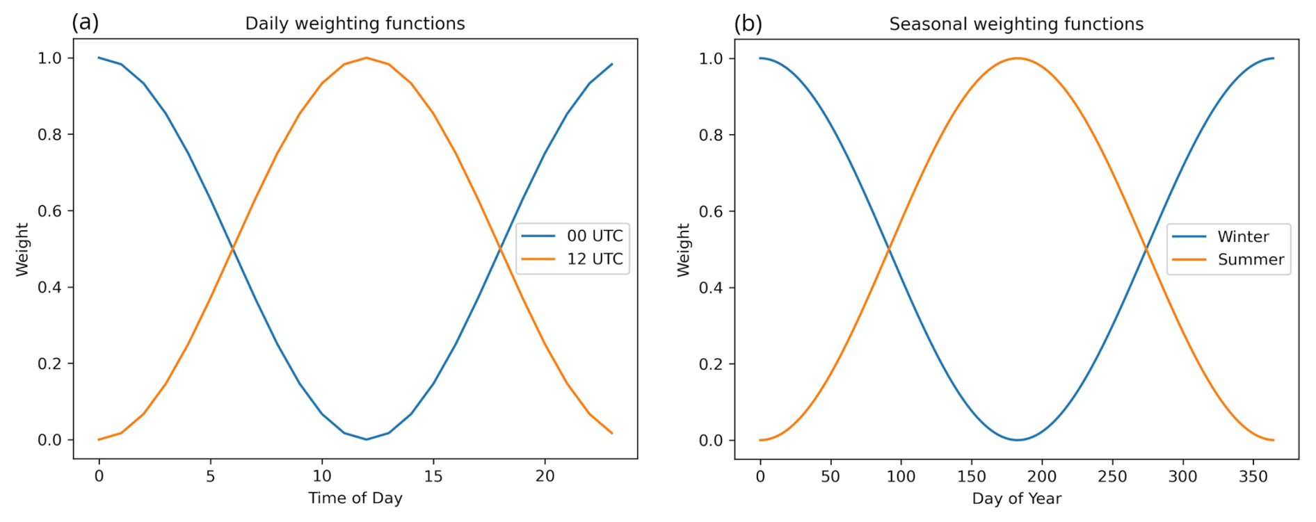
Figure 6Weighting functions for the downscaling parameters. (a) Daily weighting functions for 00:00 and 12:00 UTC parameters. (b) Weighting functions for the seasonal parameters at day number 0 (winter) and 183 (summer).
For tasmin and tasmax, no separate regressions were conducted. Instead, the relationships derived for tas were applied to each of the 12 h throughout the day (see Table 2). Weights for pr downscaling were derived based on seasonal variation only, with no diurnal dependence. In addition, a non-negative least squares approach was applied to ensure all downscaled values were non-negative.
The same weighting functions used to derive regression parameters during the overlapping time period were applied to full UERRA-HARMONIE time series, allowing parameter interpolation for any given day and time:
where hr is the analysis hour, dn is the day number of the year, wd00 and wd12 are diurnal weights, and wyw and wys are seasonal weights. These weights are then used in a linear combination of the regression parameters associated with 00:00 and 12:00 UTC, and with winter and summer, respectively:
where p is the combined regression parameter used for downscaling.
For tasmin and tasmax, each of the 12 sub-daily intervals (Table 2) was downscaled individually, using the midpoint of each interval to determine the appropriate weighting.
Downscaling of daily snow water equivalent was performed using constant weights and involved several steps. First, the snow water equivalent was downscaled from UERRA-HARMONIE using the regression-based approach described above. Subsequently, snd was estimated by dividing the downscaled snow water equivalent by the snow density interpolated from UERRA-HARMONIE to the SMHIGridClim grid. To correct for systematic differences between the distributions of downscaled and observed snow depth, a bias correction was applied using quantile mapping. This procedure included imposing an upper limit of 10 m on the downscaled snow depth, reflecting the maximum observed values, followed by sorting the observed and downscaled snow depth data to establish a lookup table with 5000 pairs evenly distributed between 0 and 10 m. The quantile mapping method then linearly interpolated between these points to map the downscaled snow depth distribution onto the observed distribution. Quantile mapping has been shown to effectively correct systematic errors in precipitation-related variables (Panofsky and Brier, 1968; Themeßl et al., 2012).
3.2 Optimal interpolation analysis
The analysis was performed with the open-source gridpp library developed by the Norwegian Meteorological Institute (https://github.com/metno/gridpp, last access: 27 August 2026). Specifically, the Python library version of gridpp was employed, which offers functions for performing analyses using optimal interpolation (OI). This technique combines a gridded first-guess field with observations to obtain a linear, minimum-error-variance estimate of the atmospheric field (Gandin, 1965). Let xa and xb denote the first guess and analysis on the grid, respectively, yo the observations, and H the operator that interpolates the first guess to the observation locations. The analysis is then
where G contains the first-guess error covariances between grid points and observation locations, S contains the corresponding covariances between observation locations, and R is the observation-error covariance matrix. Thus, gridpp does not require separate full covariance matrices as input; the required covariance information is represented by a single spatial structure function together with the ratio of observation- to first-guess-error variance.
Observation errors were assumed to be unbiased, mutually uncorrelated, and to have the same variance within each analysis configuration. Consequently,
The observation errors were also assumed to be uncorrelated with the first-guess errors. The first-guess error covariance between locations ri and rj was represented as
where ρ is the correlation function. After dividing the covariance matrices by , only the error-variance ratio
is required. Smaller values of ϵ2 therefore assign greater relative weight to the observations, whereas larger values retain more of the first guess.
The spatial correlation was modelled using the BarnesStructure class in gridpp (Barnes, 1973). To account for the reduced representativeness of observations across strong surface contrasts, the correlation function includes horizontal separation, elevation difference, and difference in land-area fraction:
where d is horizontal distance, Δz is elevation difference, and Δw is the absolute difference in land-area fraction. The parameters Dh, Dz and Dw determine the rates at which correlation decreases with horizontal distance, elevation difference and difference in land-area fraction, respectively. For each analysis configuration, the complete set of covariance-related information was therefore specified by the structure parameters (Dh, Dz, Dw) and the variance ratio ϵ2.
For the SMHIGridClim analyses, gridpp.optimal_interpolation was used with parameter max_points set to zero, allowing all observations within the localisation radius to contribute. The default maximum influence radius of BarnesStructure, equal to 3.64 times the horizontal decorrelation length Dh, was retained. It represents a permissive cut-off that excludes only observations with negligible correlation and is intended mainly to limit computational cost in very dense networks. Given the relatively sparse station network used here, the cut-off is unlikely to influence the analysis substantially, and no separate sensitivity study was conducted. The Barnes formulation was used throughout the study; alternative functional forms were not evaluated, and sensitivity of the final gridded fields to the choice of structure function therefore remains unquantified.
A cross-validation procedure was conducted to determine suitable parameter values for the error variance, the ratio between first guess and observation error variances, and the parameters governing the structure function. This procedure is implemented within gridpp, which performs the analysis using a “leave-one-out” cross-validation approach. Specifically, for each observation point, the corresponding observation is excluded from the OI analysis to estimate the error at that location. Although this error estimate may not fully represent the spatial structure of the OI analysis, it provides valuable independent information on how well the analysis fits the observations.
The optimal parameters of the structure function depend on the observation density, which varies over time. Consequently, optimal parameters were derived for selected years (1965, 1975, 1985, 1995, 2005, and 2015) within the 1961–2018 period. For the remaining years, parameters were obtained through spline interpolation, with the values for 1965 and 2015 applied to the years 1961–1964 and 2016–2018, respectively. Separate parameter sets were assigned for night and day as well as for winter and summer, employing the same weighting functions (wf) as used in the downscaling step, augmented with a 10-year wide weighting window around each reference year:
where yr corresponds to the year for which the calculation will be carried out, and yr.
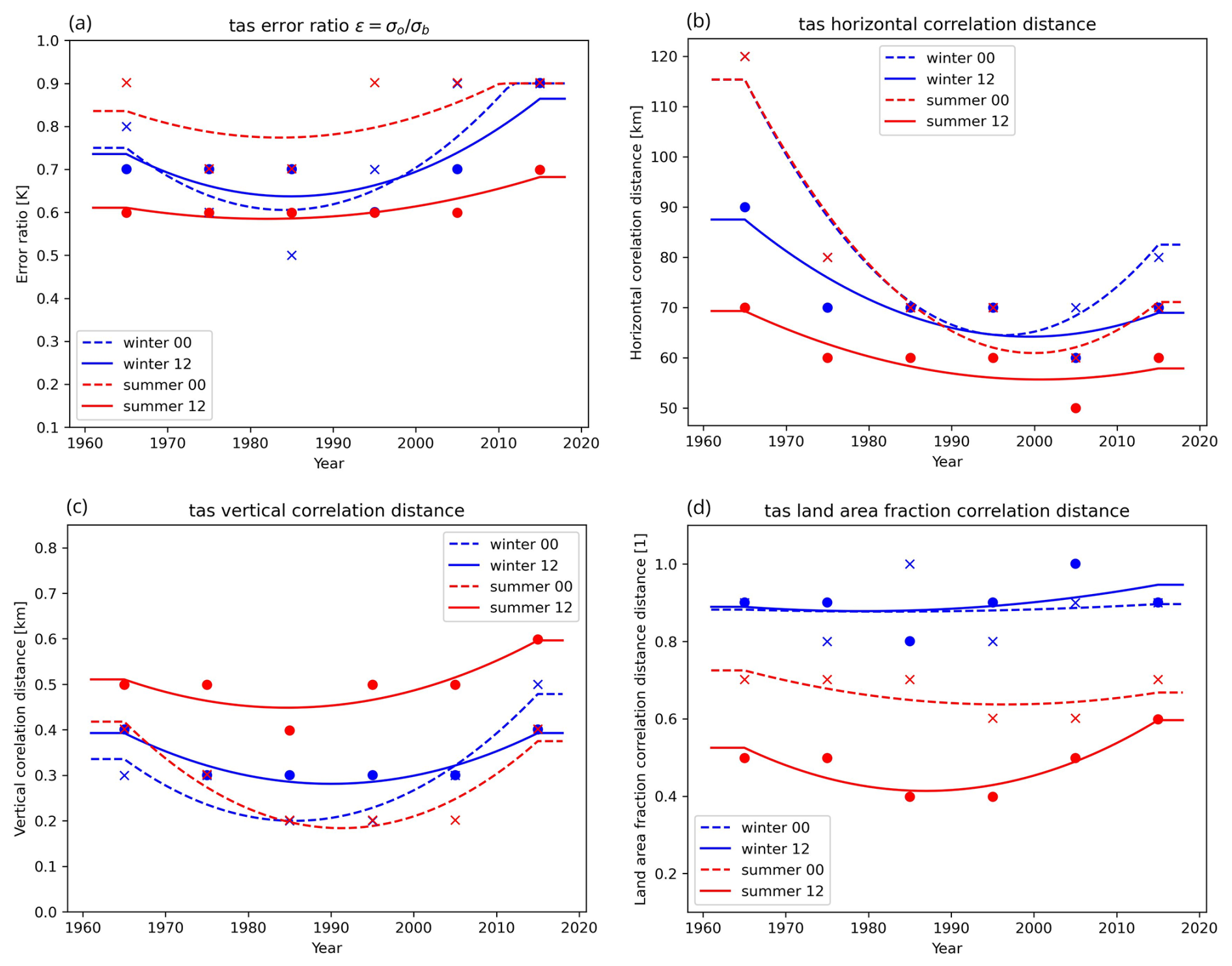
Figure 7Time interpolation of optimised gridpp parameters for tas. (a) Error variance ratio (unitless). (b) Horizontal correlation (unit: m). (c) Vertical correlation (unit: m). (d) Land area fraction correlation (unitless).
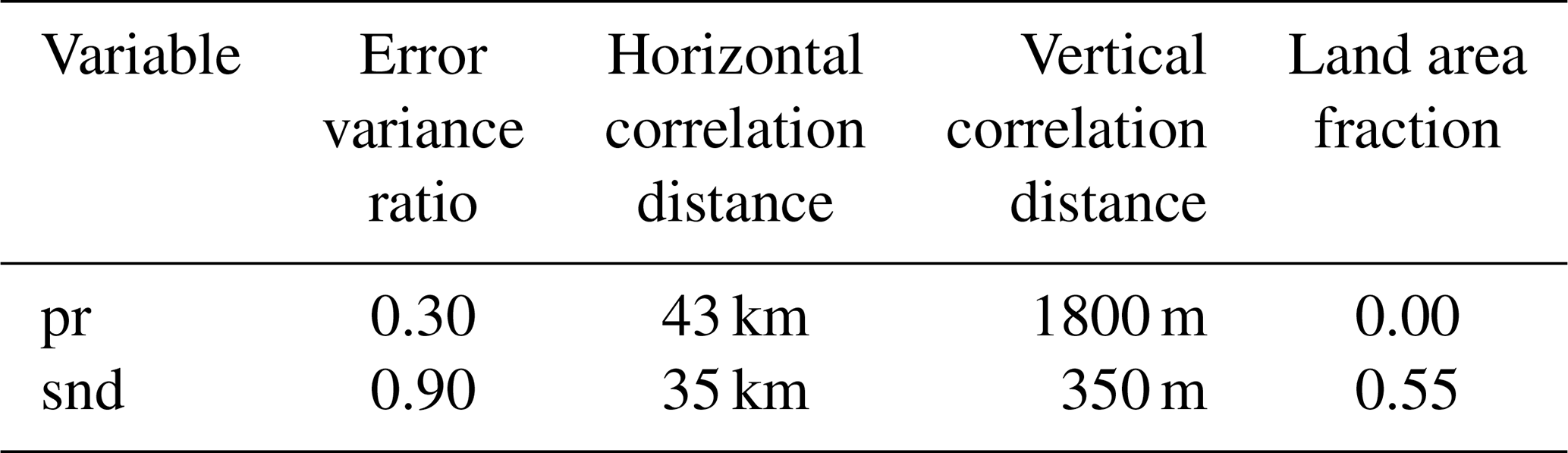
For any given year and date within the time period, parameter values were then smoothly interpolated using quadratic smoothing splines (k=2), implemented with scipy.interpolate.UnivariateSpline. The internal knots were selected adaptively by the underlying algorithm subject to a smoothing constraint of , where N is the number of fitted parameter values. Constant extrapolation was applied outside the range of the reference year. The final optimised gridpp parameters used for the temperature analysis are illustrated in Fig. 7, alongside the average number of observations. Similar procedures were followed for tasmin, tasmax, and tdps. Cross-validation during parameter selection indicated that allowing temporal variation provided some improvement over constant parameter values, but the corresponding comparison scores were not retained and the magnitude of this improvement cannot be quantified. The improvement was observed to be small, suggesting that the analysis is relatively insensitive to the precise parameter values and that some of the estimated temporal variability may reflect optimisation uncertainty or limited parameter identifiability. Allowing temporal variation may nevertheless introduce some temporal inhomogeneity. For pr and snd the optimisation yielded relatively constant parameter values across years and seasons; therefore, fixed values were used for these variables, as summarised in Table 3. The optimised parameters vary over time, as shown in Fig. 7. Their estimation may be influenced by changes in observation density and network geometry, although genuine temporal changes in the spatial covariance characteristics of the atmospheric fields may also contribute. These effects cannot be separated here, and the parameter curves should therefore be regarded as empirical analysis settings rather than direct evidence of physical covariance changes.
Table 3Optimal gridpp parameters for the analysis of daily precipitation and snow depth.
As described in Sect. 3.1, the analysis was performed using the downscaled fields as the first guess. One exception was hurs, which was not directly analysed with gridpp. Instead, it was diagnosed using the gridpp.relative_humidity function, using the analysed tas and tdps fields as inputs. This avoids applying OI directly to a variable bounded between 0 % and 100 %, whose errors depart more strongly from normality. The diagnostic transformation is nonlinear, and the resulting relative-humidity errors therefore reflect a nonlinear combination of errors in both analysed input fields.
This section describes the result from the analysis with gridpp as well as from the data processing steps. In Sect. 4.1 an overview of the final climatology data is presented in terms of difference maps between the period 1961–1990 and 1991–2018. Section 4.2–4.5 illustrates the results of the different processing steps in the analysis, starting with cross validation of the dataset with observations, followed by the result of the downscaling of UERRA-HARMONIE fields, and the analysis increments from interpolation with gridpp.
4.1 Climatologies
Figure 8 shows the resulting climatologies from SMHIGridClim in terms of maps showing the difference between the period 1991–2018 and the standard reference period 1961–1990 according to World Meteorological Organization (WMO). This gives a view of how the dataset represents changes in the variables over time. For temperature related parameters tas, tdps, tasmin and tasmax, increase is seen over almost the entire region as expected due to climate change. This increase is largest for the daily minimum temperature, with up to two degrees.
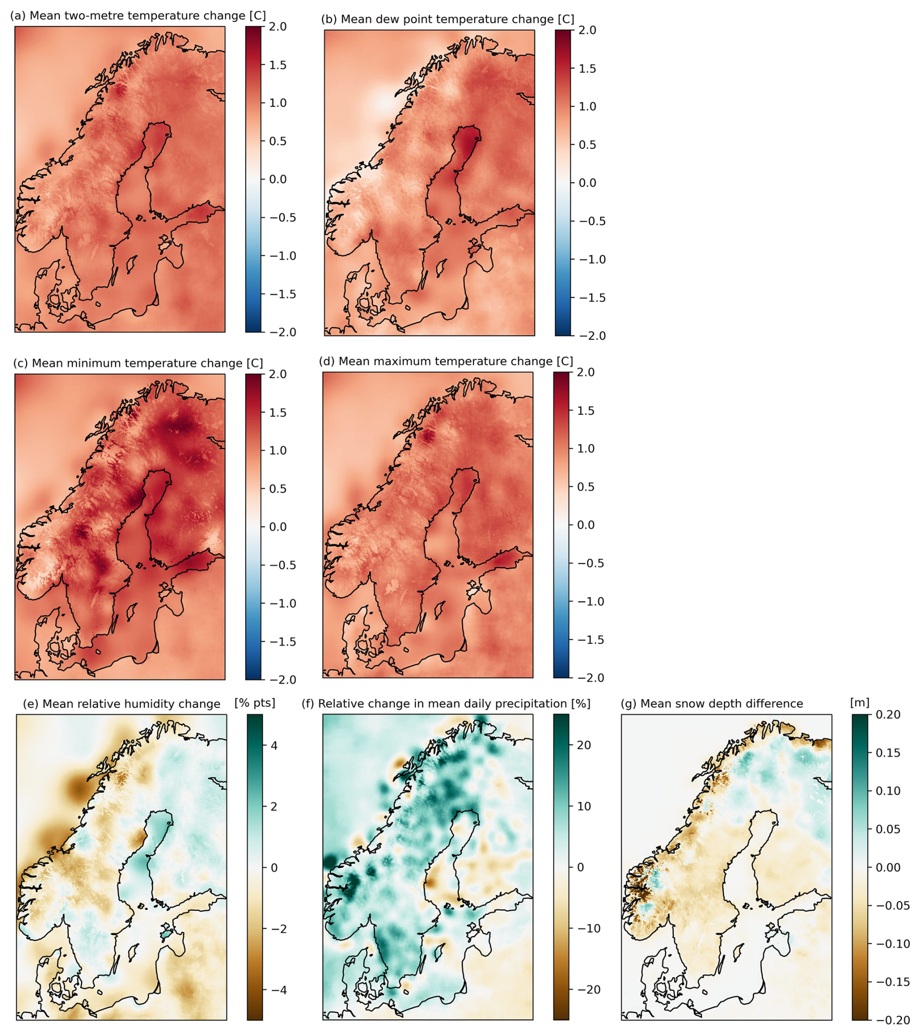
Figure 8Differences between climatologies for the time periods 1991–2018 and 1961–1990. (a) Hourly mean tas. (b) Hourly mean tdps. (c) Daily mean tasmin. (d) Daily mean tasmax. (e) Hourly mean hurs. (f) Yearly mean pr. (g) Daily mean snd.
For hurs the result is patchier and the differences between the climate periods are generally small, indicating no clear trend. Precipitation on the other hand generally shows an increase between the two periods. The snow depth generally shows a decrease, as can be expected from a warmer climate, except in northern Finland and in some small areas in the Norwegian mountains and northern Sweden.
It is important to note that SMHIGridClim is affected by inhomogeneities that may introduce artificial trends in the dataset. Discrepancies may partly be related to changes in the observation network. Also regions with complex topography present challenges for accurately representing local climate conditions in gridded datasets. Thus there is a risk that patterns shown in Fig. 8 and in the underlying data does not represent genuine climate signals and which may be artefacts related to the underlying data and methodology.
Also there are some isolated points standing out in the difference maps, clearly seen for the relative humidity and the precipitation. They are mainly located in coastal regions, especially along the Norwegian coast, for example around Lofoten. The reason for these deviations is that the contrast between land and sea is not represented by the scale of the grid used for the analysis. Thus, stations located in coastal areas, exhibit an influence on sea-covered area giving values that are less realistic. However, over Sweden, which is the focus area of this analysis, the fields look rather smooth.
4.2 Cross validation
The core validation metric for the dataset is the “leave-one-out” cross validation results that the gridpp analysis provides at each analysis time step. Therefore, cross validation results are given for the original UERRA-HARMONIE fields, the downscaled field used for first guess, and the resulting analysed fields. The exception was for hurs that was diagnosed from tdps, thus cross validation was done also for tdps. The cross-validation results for 12:00 UTC for all analysed parameters is shown in Fig. 9. Plots for other hours can be found in the dataset technical report (Andersson et al., 2021).
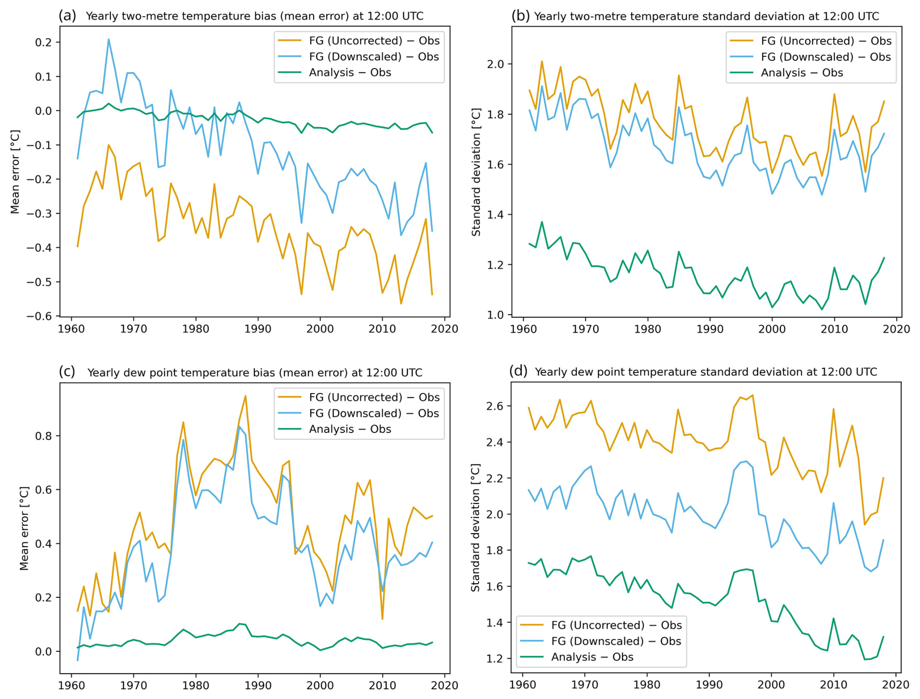
Figure 9Yearly error statistics for tas and tdps at 12:00 UTC relative to observations (Obs). Panels show (a) tas mean bias, (b) tas error standard deviation, (c) tdps mean bias, and (d) tdps error standard deviation. Curves correspond to the uncorrected UERRA-HARMONIE first guess (FG Uncorrected), the downscaled first guess (FG Downscaled), and the analysis product (Analysis). Analysis errors are evaluated using a leave-one-out cross-validation scheme.
With a few exceptions, both the downscaling of UERRA-HARMONIE fields and the analysis with gridpp improved the statistics for most parameters, in terms of decreased bias and standard deviation.
A limitation was that the temperature fields from both UERRA-HARMONIE and MEPS were shown to have too low maximum temperatures, and too high minimum temperatures, compared to the observations (Fig. 10). In addition, MEPS in general had warmer temperatures than UERRA-HARMONIE, which worsened the situation for low temperatures as the downscaling was done under the assumption that the performance of the MEPS forecast is superior to that of the UERRA-HARMONIE forecast. Below some more details about the results are discussed.
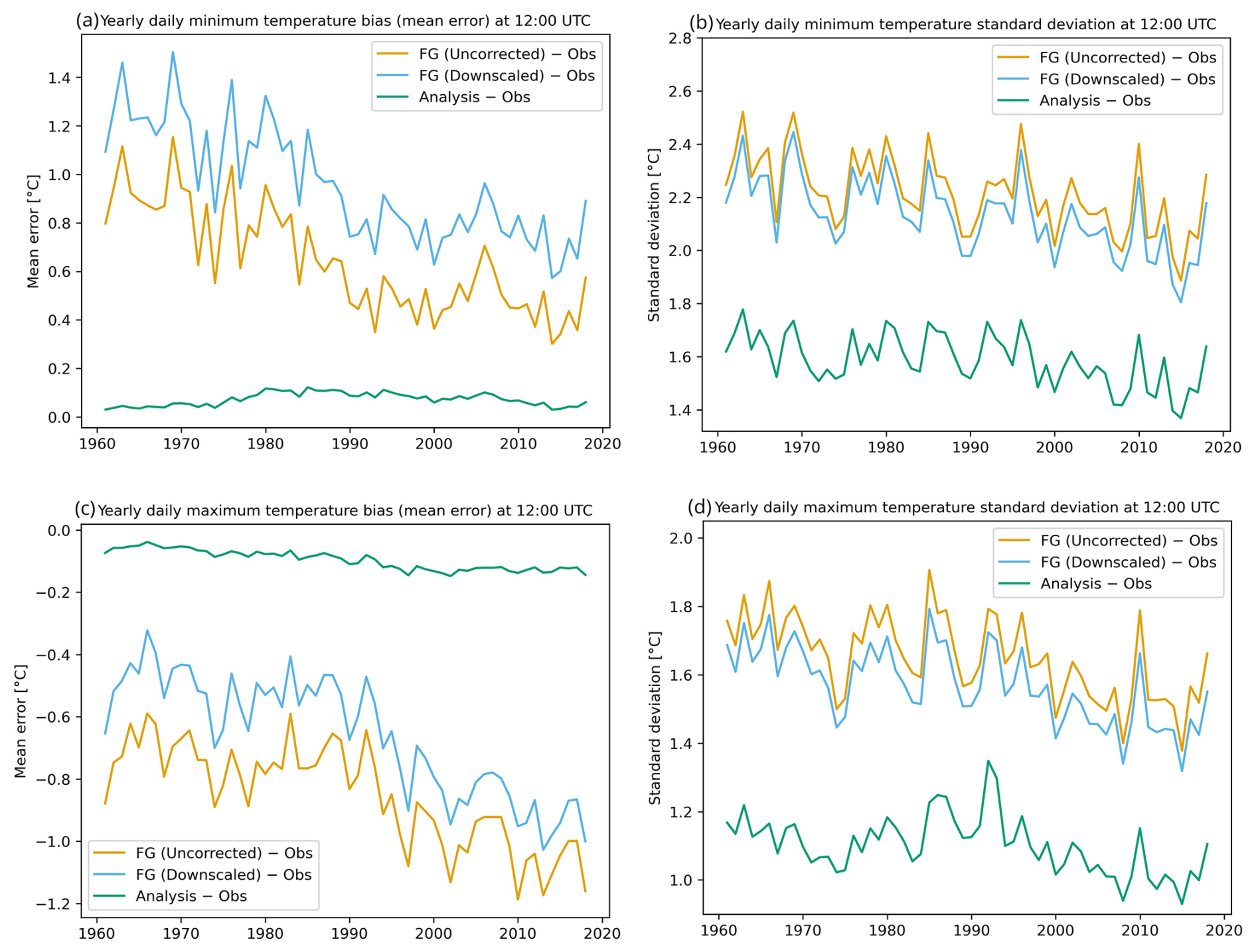
Figure 10Yearly error statistics for daily minimum and maximum temperatures (tasmin and tasmax respectively) relative to observations (Obs). Panels show (a) tasmin mean bias, (b) tasmin error standard deviation, (c) tasmax mean bias, and (d) tasmax error standard deviation. Curves correspond to the uncorrected UERRA-HARMONIE first guess (FG Uncorrected), the downscaled first guess (FG Downscaled), and the analysis product (Analysis). Analysis errors are evaluated using a leave-one-out cross-validation scheme.
For two-metre temperature (Fig. 9a and b), a negative bias of the UERRA-HARMONIE forecast valid at 12:00 UTC means that the model fields are generally too cold. Here, the downscaling improves on both the bias and the standard deviation. As a result, the total error in terms of the standard deviation is also improved by the downscaling. The statistics for other hours follow a similar pattern, with the exception that at 00:00 UTC the downscaling actually increases an already positive bias even more (not shown).
Furthermore, the first guess entering the optimal interpolation shows a positive bias that seems to grow towards the end of the time period. There is however a slight improvement in the standard deviation of the UERRA-HARMONIE data over time. The added number of observations towards the end of the period does not lead to any significant improvement on the analysis error. An increasing bias in the first guess is also seen for several other parameters, the reason for this has not been investigated further.
For the dew point temperature (Fig. 9c and d), the downscaling improves the standard deviation but does not significantly change the systematic overestimation (positive bias) of tdps in the UERRA-HARMONIE forecasts valid at 12:00 UTC. During the night (not shown here) the downscaling helps improving a negative bias at the end of the time period, although it overcompensates somewhat in the early years.
For the daily minimum temperature (Fig. 10a and b), the downscaling results in only slightly lower standard deviation and hardly any difference in the bias. At the same time the positive bias is increasing. Although the downscaling did not improve the fields for first guess, the RMSE did not increase notably, and the analysis compensates for this in the final results.
Also, there is a trend towards lower standard deviation values over time for the first guess for minimum temperature. This trend is not carried over to the analysis to the same extent, even though it should be further strengthened by the increase in observations towards the end of the period.
For the daily maximum temperature (Fig. 10c and d), the downscaling procedure results in a small improvement, both with respect to bias and standard deviation. A dip in the number of available observations around the 1980s and 1990s (not shown) seems to be reflected in the standard deviation of the analysis. Also, the trend towards lower standard deviation values, as was seen for the daily minimum, is not as pronounced for the daily maximum.
For the relative humidity (Fig. 11a and b), which was calculated from the downscaling of tas and tdps, thus no observations of hurs enter the analysis. Instead, the comparison is done to hurs values calculated from co-located observations of tas and tdps.
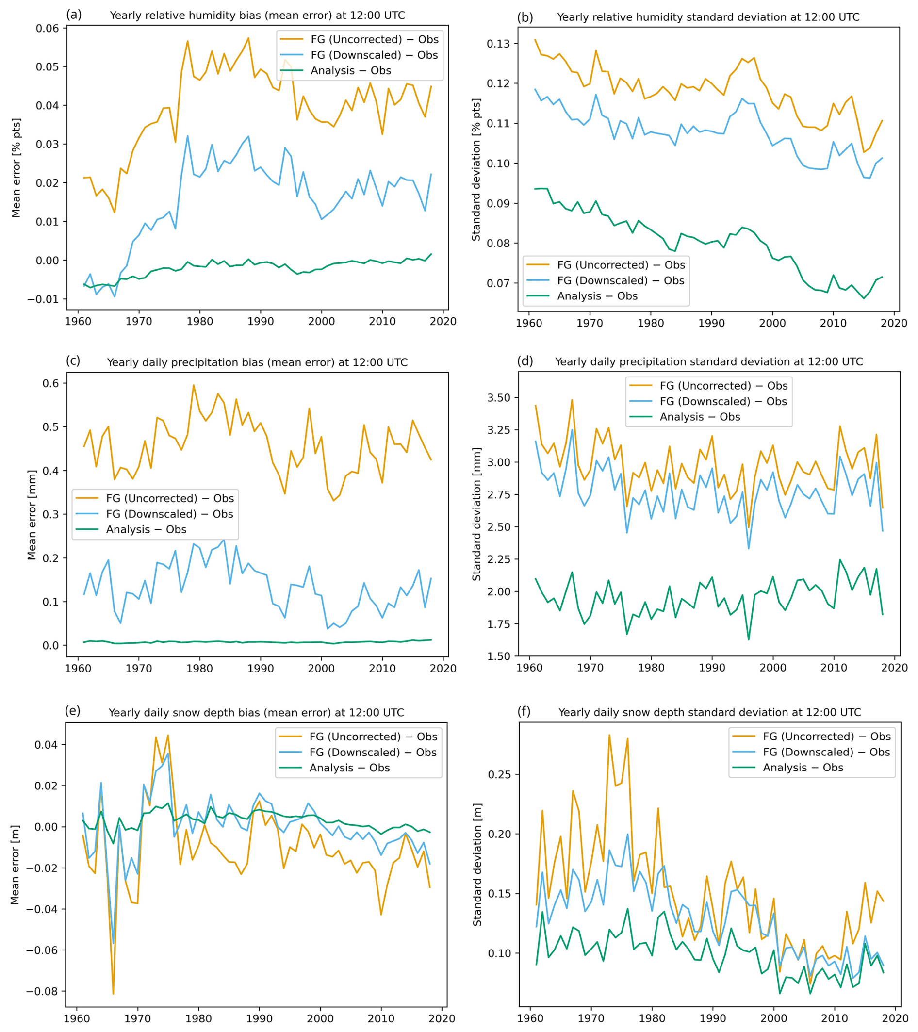
Figure 11Yearly error statistics for relative humidity, daily precipitation and snow depth relative to observations (Obs). Panels show (a) hurs mean bias, (b) hurs error standard deviation, (c) pr mean bias, (d) pr error standard deviation, (e) snd mean bias and (f) snd error standard deviation. Curves correspond to the uncorrected UERRA-HARMONIE first guess (FG Uncorrected), the downscaled first guess (FG Downscaled), and the analysis product (Analysis). Analysis errors are evaluated using a leave-one-out cross-validation scheme.
Here, although the downscaling clearly adds value compared to the UERRA-HARMONIE forecasts, the analysis cannot fully compensate for the bias in the first guess and one can see a small increasing trend also in the bias of the analysis.
Error statistics for the daily precipitation (Fig. 11c and d) generally show the expected improvement, a bias close to zero and a clear improvement on top of the first guess. The number of observations peaks during the 1980s and 1990s (see Fig. 3), this coincides with an improved standard deviation for the first guess but is not seen clearly in the standard deviation of the analysis.
Finally, for the daily snow cover (Fig. 11e and f), the downscaling of the UERRA-HARMONIE forecasts most of the time results in lower standard deviation as well as a reduction in bias.
There is no clear connection between the error in the first guess and the yearly mean snow depth (not shown), nor with its 95th percentile. The reason for the large errors in the UERRA-HARMONIE snow fields during the 1970s has not been studied. There is no clear connection between the number of observations and the standard deviation of the analysis. The analysis of daily snow cover shows added value from the first guess, at least during the first and last 15 years.
4.3 Comparison with other Nordic gridded datasets
SMHIGridClim was further evaluated by comparing cross validation results for SMHIGridClim with values found in the literature for two comparable datasets from the Nordic neighbour institutes Finland and Norway (Table 4). The cross-validation results are mostly similar, especially SMHIGridClim and seNorge (Lussana et al., 2018, 2019). FMI_ClimGrid (Aalto et al., 2016) shows slightly better performance for the available variables in this dataset, which might be explained by more challenging topography to be represented for the Swedish and Norwegian datasets. Thus, SMHIGridClim provides a high-resolution gridded dataset, with a quality on par with similar datasets from other institutes.
Table 4Mean RMSE for hourly tas and daily tasmin, tasmax, pr, and snd for three Nordic gridded datasets.
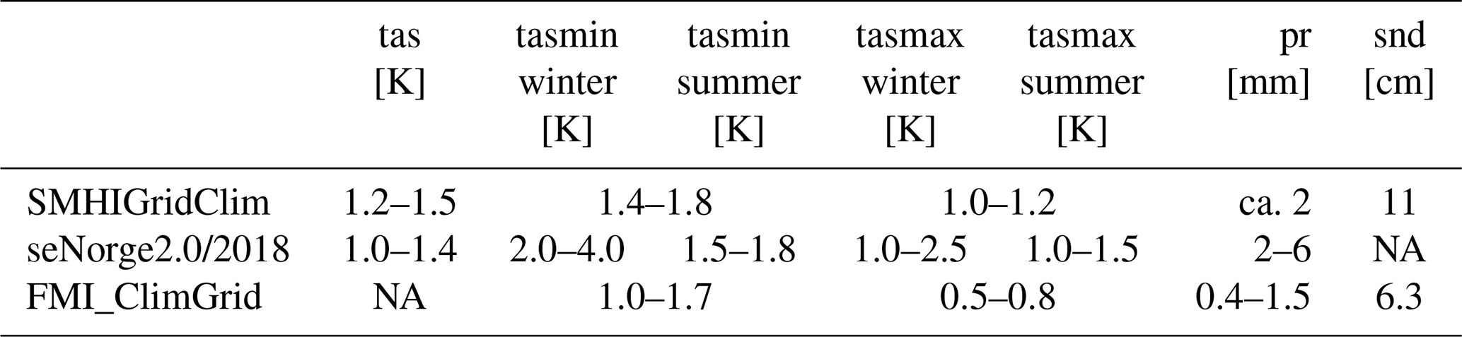
NA stands for not available.
In addition to the listed datasets, there are many well-known widely used reanalysis data, such as ERA5 (Hersbach et al., 2020) and CERRA (Schimanke et al., 2021). However, it is difficult to do a valid comparison as there exists no cross validation results. Also, the resolution of these datasets are many times coarser than in SMHIGridClim (∼31 and 5.5 km respectively).
4.4 Spatial structures of downscaling
In addition to the cross validation results presented in Sect. 4.2, the spatial behaviour of the processing steps was investigated by difference maps. For the difference maps showing the effect of the downscaling of UERRA-HARMONIE, the fields first had to be interpolated to the SMHIGridClim grid using bilinear interpolation. The downscaling procedure results in fields that fit the patterns in the corresponding MEPS fields during the years 2016–2018. The assumption for the downscaling is that the performance of the MEPS forecast is superior to that of the UERRA-HARMONIE forecast.
In Fig. 12, examples of the downscaling effect for one summer month, winter month and 12:00 and 00:00 UTC are shown for two-metre temperature and for daily precipitation.
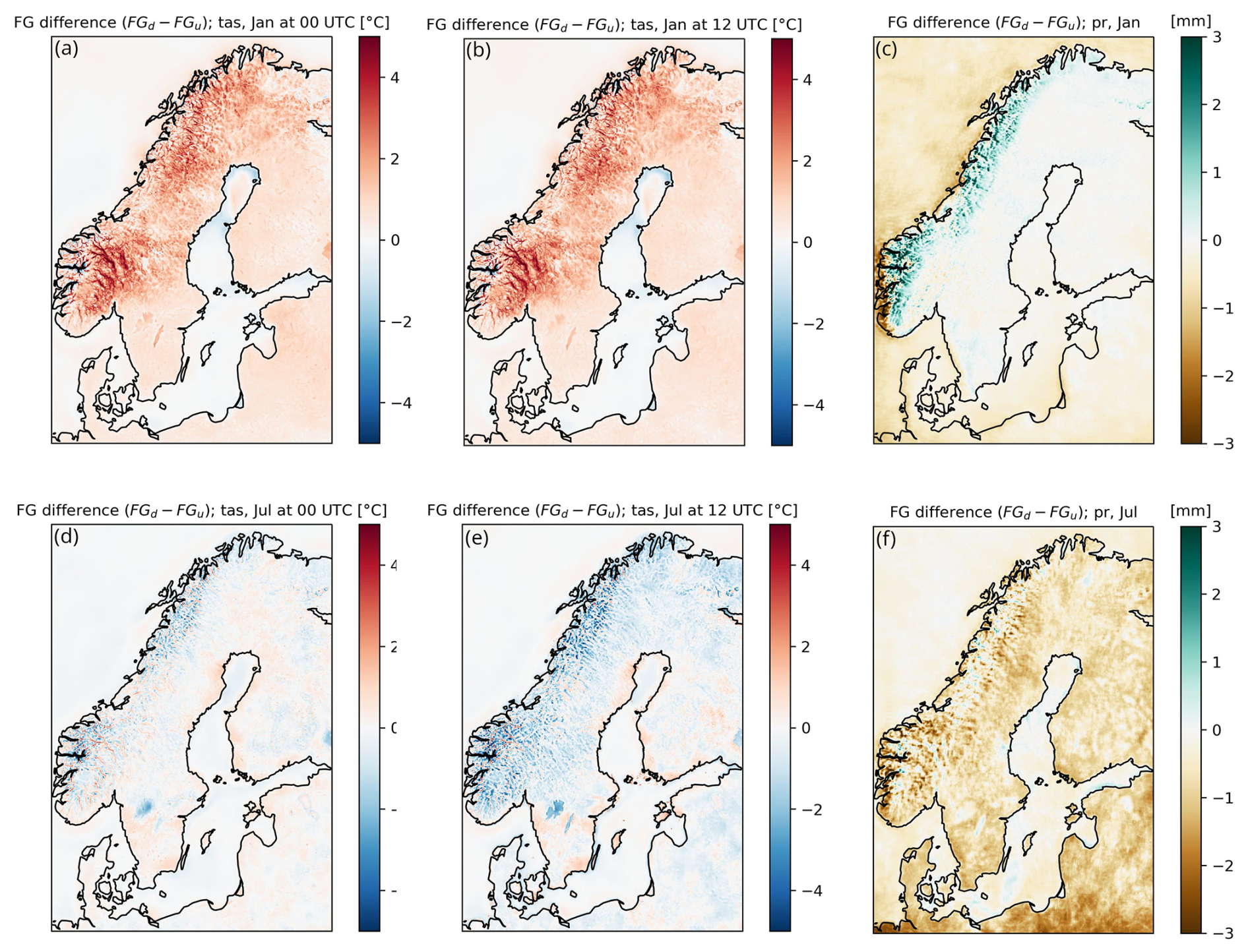
Figure 12Mean differences between tas and pr from the downscaled (FGd) and original uncorrected UERRA-HARMONIE fields (FGu) respectively. (a) tas for January 00:00 UTC. (b) tas for January 12:00 UTC. (c) pr during January. (d) tas for July 00:00 UTC. (e) tas for July 12:00 UTC. (f) pr during July.
For two-metre temperature, it was shown earlier, in the cross-validation results, that the downscaling helped to reduce the negative bias in temperatures in UERRA-HARMONIE. Looking into the downscaling in more details, in the winter (represented by January) the downscaling results in higher temperatures, both during night and day (Fig. 12). In the summer (July) on the other hand, it is the other way around, with the downscaling mostly producing colder temperatures, especially in the mountains during the day.
Note that the downscaling makes the two largest lakes in Sweden, Vänern and Vättern, slightly warmer during winter and noticeably colder during summer.
During the winter the downscaling intensifies the precipitation in the mountains. For the summer period, the downscaling instead results in a general decrease in the daily precipitation. For snow depth, downscaling increases the depth for most places in the analysed area.
4.5 Spatial structures of analysis increments
Analysis increments are here shown as the difference between the analysis and the first guess, given by the downscaled UERRA-HARMONIE fields. Thus, they show the influence of the interpolation with gridpp. Note that this means that positive values in the maps indicate that the first guess was too low and vice versa for negative values. Ideally the distribution of the analysis increments should follow a normal distribution with zero mean.
Again, using tas as example, during the winter noon the analysis results in a systematic increase of the temperature while it is the other way around during the summer night.
This can be compared to the differences between the downscaled and original UERRA-HARMONIE fields shown in Fig. 12. The downscaling resulted in warmer fields during the winter days but not warm enough to fit the observations. For the summer night the downscaling was rather neutral indicating that both MEPS and UERRA-HARMONIE have a positive bias for that period. For minimum and maximum temperatures (not shown), the analysis changes the maximum to be warmer and the minimum to be colder than what is suggested by the first guess. As discussed earlier for the cross-validation results (Figs. 9–11), this shift is compensating for the downscaling towards the opposite direction in temperature caused by the MEPS model, in order to fit the first guess to the observations.
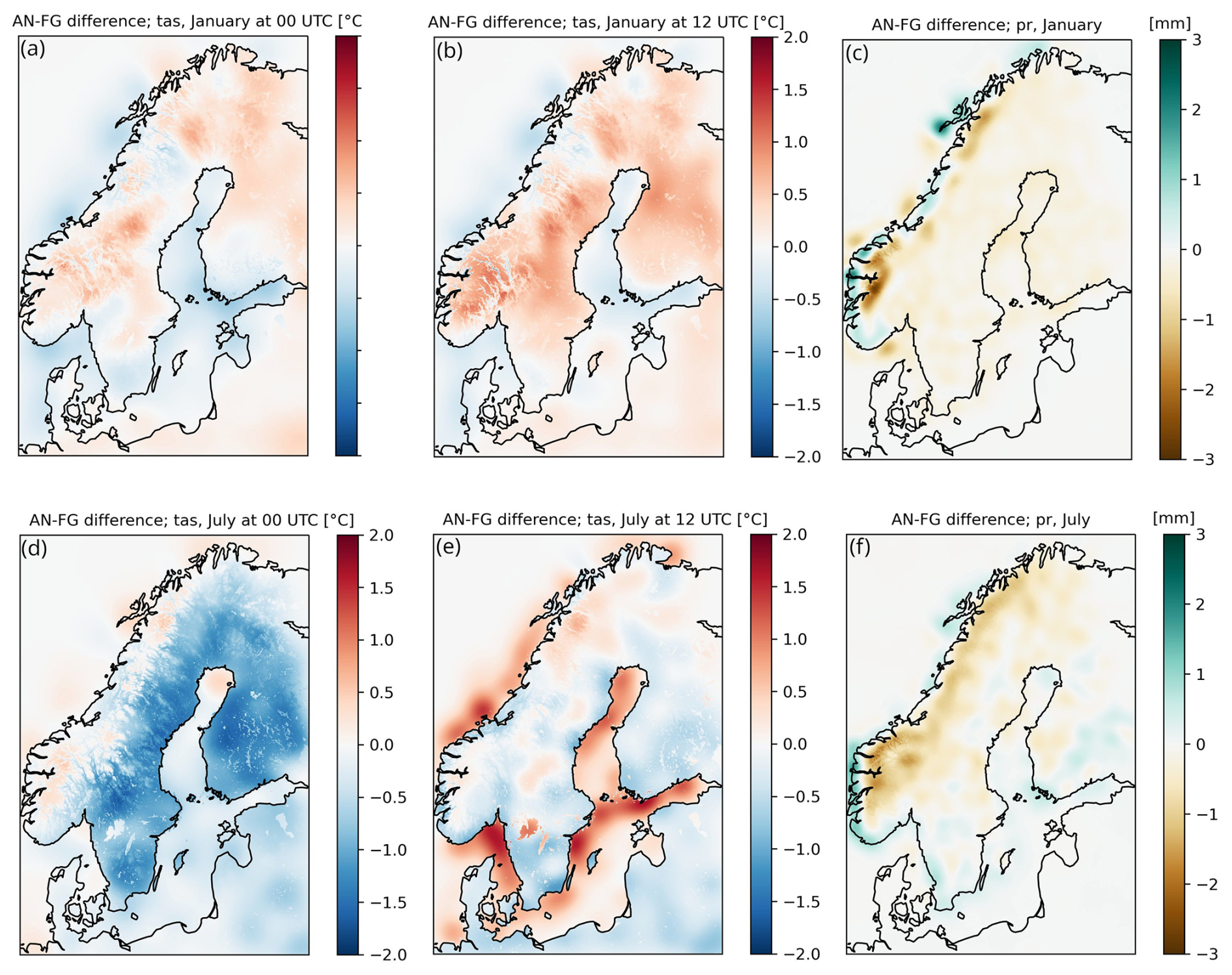
Figure 13Mean analysis increments (AN-FG) for tas and pr during January (top row) and July (bottom row). (a) tas for January 00:00 UTC, (b) tas for January 12:00 UTC, (c) pr during January, (d) tas for July 00:00 UTC, (e) tas for July 12:00 UTC and (f) pr during July.
The analysis increments for the daily precipitation show in general small changes but indicate that the first guess has too much precipitation, especially in the Norwegian mountain regions. During summer, the first guess has too little precipitation along the south-west Norwegian coast and there is also a slight tendency that the first guess underestimates the precipitation along the Swedish west coast during the summer season.
The SMHIGridClim dataset for the years 1961–2018 is available at https://doi.org/10.7910/DVN/ZFZL6K (Andersson et al., 2025). Work to extend the dataset to present day is currently being performed at SMHI.
A number of things should be kept in mind using this kind of modelled climatological data. Although the horizontal grid resolution of SMHIGridClim is 2.5 km, the effective resolution is larger due to the underlying model fields. With effective resolution we mean the resolution that has actual meaningful information. For MEPS at 2.5 km the effective resolution is likely about a magnitude larger. Due to the nature of numerical solutions and parametrizations, the model effective resolution degrades to several grid spacings (Abdalla et al., 2013). This also affects the result of the evaluation of analysis increments as comparison was not done at its actual effective resolution.
Although SMHIGridClim is produced to be a high-resolution climate dataset, it is not appropriate to use for detailed studies of trends as it suffers from inhomogeneity. The dataset is based on UERRA-HARMONIE reanalysis topped with observations. UERRA-HARMONIE is based on a frozen model system which means that it does not change over time, but the observations show large variations in frequency and density and sometimes data quality. Furthermore, the parameters used in the analysis with gridpp were allowed to change in order to adapt to the observations available over time. This could introduce false trends in data. To minimise this influence, one could have limited the analysis to only include long-term observations, but this would dramatically have limited the information available for the overall analysis, and therefore the quality.
The changing observation network leads to variation in data quality over time. In general, there are more observations available during the 6 hourly cycles: 06:00, 12:00, 18:00 and 00:00 UTC, followed by the 3 hourly: 06:00, 09:00, 12:00, 15:00, 18:00, 21:00 and 00:00 UTC, followed by the hourly. Also, there are less observations back in time. However, there are deviations from this so the observation density should be checked to conclude how it affects a specific study with regards to time period and region of interest. The amount of available observations differs widely over the analysed region, and the analysis is only truly valid for Sweden, Finland and Norway where national data was provided. Results are probably most reliable for Sweden where we had the best knowledge of observation quality, and less problems with steep topography and fractal coastlines like in Norway. Over water surfaces, and some land regions, the analysis contains no observations, and is therefore based on the downscaled version of the UERRA-HARMONIE reanalysis only.
Catching extreme events in the dataset is also challenging. Although downscaling is done at an hourly basis, the underlying data field from UERRA-HARMONIE has a rather coarse resolution of 11 km. Also, the downscaling is static at 00:00 and 12:00 UTC and is based on linear regression, thus it strives towards the best fit with the mean error as target. For extreme precipitation also, the fact that optimal interpolation is based on a normal distribution is problematic because this will not be representative for large precipitation events. Furthermore, the probabilities of no precipitation, light precipitation, and heavy rainfall or snowfall differ substantially. The result is that precipitation is smeared out, and extreme events not well represented. Thus, these occasions should in the future be handled separately in the analysis with gridpp to improve the result.
There is ongoing work to develop SMHIGridClim. The development includes a switch to titanlib instead of TITAN, adding wind speed as a new variable, and switch the first guess to CERRA (Schimanke et al., 2021) instead of its predecessor UERRA-HARMONIE. CERRA has the same domain as UERRA-HARMONIE, although the horizontal grid resolution is 5.5 km instead of 11 km. At present, CERRA data are available from September 1984 to May 2026, with near-real-time updates provided at a latency of approximately 3.5 months. The CERRA back extension, covering the period from September 1960 to August 1984, is not yet available and is expected to be released in 2027. There is also a plan to include observations from Denmark, Estonia, Latvia, and Lithuania in SMHIGridClim, which has been collected. Furthermore, a more thorough comparison between different gridded data sets would be of interest.
SA organized the project and wrote the manuscript. MN organized the project and wrote the manuscript. TL downscaled the original UERRA-HARMONIE fields, and performed the analysis with gridpp. PS preprocessed observation data and performed the quality control with the TITAN software. SeS fetched observation data from different data sources and meteorological institutes. MZ helped with evaluation and wrote the manuscript. LB contributed as the initiator of the study and with expertise. All authors contributed to the manuscript writing.
The contact author has declared that none of the authors has any competing interests.
Publisher's note: Copernicus Publications remains neutral with regard to jurisdictional claims made in the text, published maps, institutional affiliations, or any other geographical representation in this paper. The authors bear the ultimate responsibility for providing appropriate place names. Views expressed in the text are those of the authors and do not necessarily reflect the views of the publisher.
We acknowledge Mariken Homleid (MetNorway) and Viivi Kallio-Myers (FMI) for providing observational datasets and Cristian Lussana (MetNorway) for support with TITAN.
The publication of this article was funded by the Swedish Research Council, Forte, Formas, and Vinnova.
This paper was edited by Andrea Lammert and reviewed by two anonymous referees.
Aalto, J., Pirinen, P., and Jylhä, K.: New gridded daily climatology of Finland: Permutation-based uncertainty estimates and temporal trends in climate, J. Geophys. Res.-Atmos., 121, 3807–3823, https://doi.org/10.1002/2015JD024651, 2016.
Abdalla, S., Isaksen, L., Janssen, P. A. E. M., and Wedi, N.: Effective spectral resolution of ECMWF atmospheric forecast models, ECMWF Newslett., 137, 19–22, https://doi.org/10.21957/rue4o7ac, 2013.
Andersson, S., Bärring, L., Landelius, T., Samuelsson, P., and Schimanke, S.: SMHI Gridded Climatology, SMHI – Swedish Meteorological and Hydrological Institute, 61 pp., https://urn.kb.se/resolve?urn=urn:nbn:se:smhi:diva-6192 (last access: 9 November 2026), 2021.
Andersson, S., Norman, M., Landelius, T., Samuelsson, P., Schimanke S., Zahid M., and Bärring, L.: SMHIGridClim, 2.5 km resolution gridded climatology of Fennoscandia, Harvard Dataverse [data set], https://doi.org/10.7910/DVN/ZFZL6K, 2025.
Barnes, S. L.: Mesoscale objective map analysis using weighted time series observations, NOAA Tech. Memo. ERL NSSL-62, 60 pp., NOAA, https://repository.library.noaa.gov/view/noaa/17647 (last access: 9 November 2026), 1973.
Båserud, L., Lussana, C., Nipen, T. N., Seierstad, I. A., Oram, L., and Aspelien, T.: TITAN automatic spatial quality control of meteorological in-situ observations, Adv. Sci. Res., 17, 153–163, https://doi.org/10.5194/asr-17-153-2020, 2020.
Bazile, E., Abida, R., Verelle, A., Le Moigne, P., and Szczypta, C.: Report for the 55 years MESCAN-SURFEX re-analysis, Copernicus Climate Change Service, https://uerra.eu/component/dpattachments/?task=attachment.download&id=399 (last access: 18 November 2024), 2017.
Brohan, P., Kennedy, J. J., Harris, I., Tett, S. F. B., and Jones, P. D.: Uncertainty estimates in regional and global observed temperature changes: A new data set from 1850, J. Geophys. Res., 111, D12106, https://doi.org/10.1029/2005JD006548, 2006.
Caesar, J., Alexander, L., and Vose, R.: Large-scale changes in observed daily maximum and minimum temperatures: Creation and analysis of a new gridded data set, J. Geophys. Res., 111, D05101, https://doi.org/10.1029/2005JD006280, 2006.
Copernicus Climate Change Service, Climate Data Store: UERRA regional reanalysis for Europe on single levels from 1961 to 2019, Copernicus Climate Change Service (C3S) Climate Data Store (CDS) [data set], https://doi.org/10.24381/cds.32b04ec5"10.24381/cds.32b04ec5, 2019.
Cornes, R.C., van der Schrier, G., van den Besselaar, E. J. M., and Jones, P. D.: An ensemble version of the E-OBS temperature and precipitation data sets, J. Geophys. Res.-Atmos., 123, 9391–9409, https://doi.org/10.1029/2017JD028200, 2018.
Dee, D. P., Uppala, S. M., Simmons, A. J., Berrisford, P., Poli, P., Kobayashi, S., Andrae, U., Balmaseda, M. A., Balsamo, G., Bauer, P., Bechtold, P., Beljaars, A. C. M., van de Berg, L., Bidlot, J., Bormann, N., Delsol, C., Dragani, R., Fuentes, M., Geer, A. J., Haimberger, L., Healy, S. B., Hersbach, H., Hólm, E. V., Isaksen, L., Kållberg, P., Köhler, M., Matricardi, M., McNally, A. P., Monge-Sanz, B. M., Morcrette, J.-J., Park, B.-K., Peubey, C., de Rosnay, P., Tavolato, C., Thépaut, J.-N., and Vitart, F.: The ERA-Interim reanalysis: Configuration and performance of the data assimilation system, Q. J. Roy. Meteorol. Soc., 137, 553–597, https://doi.org/10.1002/qj.828, 2011.
Essou, G. R. C., Arsenault, R., and Brissette, F. P.: Comparison of climate datasets for lumped hydrological modeling over the continental United States, J. Hydrol., 537, 334–345, https://doi.org/10.1016/j.jhydrol.2016.03.063, 2016.
Førland, E. J., Hanssen-Bauer, I., Jónsson, T., Kern-Hansen, C., Nordli, P. Ø., Tveito, O. E., and Laursen, E. V.: Twentieth-century variations in temperature and precipitation in the Nordic Arctic, Polar Rec., 38, 203–210, https://doi.org/10.1017/S0032247400017721, 2002.
Fountain, A. G., Campbell, J. L., Schuur, E. A. G., Stammerjohn, S. E., Williams, M. W., and Ducklow, H. W.: The disappearing cryosphere: Impacts and ecosystem responses to rapid cryosphere loss, BioScience, 62, 405–415, https://doi.org/10.1525/bio.2012.62.4.11, 2012.
Frogner, I.-L., Singleton, A. T., Køltzow, M. Ø., and Andrae, U.: Convection-permitting ensembles: Challenges related to their design and use, Q. J. Roy. Meteorol. Soc., 145, 90–106, https://doi.org/10.1002/qj.3525, 2019.
Gandin, L. S.: Objective analysis of meteorological fields, Translated from Russian, Jerusalem (Israel Program for Scientific Translations), Q. J. Roy. Meteorol. Soc., 92, 447, https://doi.org/10.1002/qj.49709239320, 1965.
Grusson, Y., Wesström, I., and Abraham, J.: Impact of climate change on Swedish agriculture: Growing season rain deficit and irrigation need, Agr. Water Manage., 251, 106858, https://doi.org/10.1016/j.agwat.2021.106858, 2021.
Harris, I., Jones, P. D., Osborn, T. J., and Lister, D. H.: Updated high-resolution grids of monthly climatic observations – the CRU TS4.05 dataset, Int. J. Climatol., 40, 5280–5292, https://doi.org/10.1002/joc.3711, 2020.
Haylock, M. R., Hofstra, N., Klein Tank, A. M. G., Klok, E. J., Jones, P. D., and New, M.: A European daily high-resolution gridded data set of surface temperature and precipitation for 1950–2006, J. Geophys. Res.-Atmos., 113, D20119, https://doi.org/10.1029/2008JD010201, 2008.
Hersbach, H., Bell, B., Berrisford, P., Hiahara, S., Horányi, A., Muñoz-Sabater, J., Nicolas, J., Peubey, C., Radu, R., Schepers, D., Simmons, A., Soci, C., Abdalla, S., Abellan, X., Balsamo, G., Bechtold, P., Biavati, G., Bidlot, J., Bonavita, M., De Chiara, G., Dahlgren, P., Dee, D., Diamantakis, M., Dragani, R., Flemming, J., Forbes, R., Fuentes, M., Geer, A., Haimberger, L., Healy, S., Hogan, R. J., Hólm, E., Janisková, M., Keeley, S., Laloyaux, P., Lopez, P., Lupu, C., Radnoti, G., de Rosnay, P., Rozum, I., Vamborg, F., Villaume, S., and Thépaut, J.-N.: The ERA5 global reanalysis, Q. J. Roy. Meteorol. Soc., 146, 1999–2049, https://doi.org/10.1002/qj.3803, 2020.
IPCC: Summary for policymakers, in Climate Change 2013: The Physical Science Basis, in: Contribution of Working Group I to the Fifth Assessment Report of the Intergovernmental Panel on Climate Change, edited by: Stocker, T. F., Qin, D., Plattner, G.-K., Tignor, M., Allen, S. K., Boschung, J., Nauels, A., Xia, Y., Bex, V., and Midgley, P. M., Cambridge Univ. Press, Cambridge, UK, and New York, 3–29, https://www.ipcc.ch/site/assets/uploads/2018/02/WG1AR5_SPM_FINAL.pdf (last access: 9 November 2026), 2013.
IPCC: Sixth Assessment Report (AR6): The Physical Science Basis, Intergovernmental Panel on Climate Change, https://www.ipcc.ch/report/ar6/wg1/ (last access: 13 November 2024), 2021.
Klein Tank, A. M. G., Wijngaard, J. B., Können, G. P., Böhm, R., Demarée, G., Gocheva, A., Mileta, M., Pashiardis, S., Hejkrlik, L., Kern-Hansen, C., Heino, R., Bessemoulin, P., Müller-Westermeier, G., Tzanakou, M., Szalai, S., Pálsdóttir, T., Fitzgerald, D., Rubin, S., Capaldo, M., Maugeri, M., Leitlass, A., Bukantis, A., Aberfeld, R., van Engelen, A. F. V., Forland, E., Mietus, M., Coelho, F., Mares, C., Razuvaev, V., Nieplova, E., Cegnar, T., Antonio López, J., Dahlström, B., Moberg, A., Kirchhofer, W., Ceylan, A., Pachaliuk, O., Alexander, L. V., and Petrovic, P.: Daily dataset of 20th-century surface air temperature and precipitation series for the European Climate Assessment, Int. J. Climatol., 22, 1441–1453, https://doi.org/10.1002/joc.773, 2002.
Klok, E. J. and Klein Tank, A. M. G.: Updated and extended European dataset of daily climate observations, Int. J. Climatol., 29, 1182–1191, https://doi.org/10.1002/joc.1779, 2009.
Le Moigne, P., Besson, F., Martin, E., Boé, J., Boone, A., Decharme, B., Etchevers, P., Faroux, S., Habets, F., Lafaysse, M., Leroux, D., and Rousset-Regimbeau, F.: The latest improvements with SURFEX v8.0 of the Safran–Isba–Modcou hydrometeorological model for France, Geosci. Model Dev., 13, 3925–3946, https://doi.org/10.5194/gmd-13-3925-2020, 2020.
Lind, P., Belušić, D., Médus, E., Dobler, A., Pedersen, R. A., Wang, F., Matte, D., Kjellström, E., Landgren, O., Lindstedt, D., Christensen, O. B., and Christensen, J. H.: Climate change information over Fenno-Scandinavia produced with a convection-permitting climate model, Clim. Dynam., 61, 519–541, https://doi.org/10.1007/s00382-022-06589-3, 2023.
Lussana, C., Uboldi, F., and Salvati, M. R.: A spatial consistency test for surface observations from mesoscale meteorological networks, Q. J. Roy. Meteorol. Soc., 136, 1075–1088, https://doi.org/10.1002/qj.622, 2010.
Lussana, C., Saloranta, T., Skaugen, T., Magnusson, J., Tveito, O. E., and Andersen, J.: seNorge2 daily precipitation, an observational gridded dataset over Norway from 1957 to the present day, Earth Syst. Sci. Data, 10, 235–249, https://doi.org/10.5194/essd-10-235-2018, 2018.
Lussana, C., Tveito, O. E., Dobler, A., and Tunheim, K.: seNorge_2018, daily precipitation and temperature datasets over Norway, Earth Syst. Sci. Data, 11, 1331–1351, https://doi.org/10.5194/essd-11-1531-2019, 2019.
Mankin, K. R., Mehan, S., Green, T. R., and Barnard, D. M.: Review of Gridded Climate Products and Their Use in Hydrological Analyses Reveals Overlaps, Gaps, and Need for More Objective Approach to Model Forcings, Hydrol. Earth Syst. Sci., 29, 85–108, https://doi.org/10.5194/hess-29-85-2025, 2025.
Monteiro, D. and Morin, S.: Multi-decadal analysis of past winter temperature, precipitation and snow cover data in the European Alps from reanalyses, climate models and observational datasets, The Cryosphere, 17, 3617–3660, https://doi.org/10.5194/tc-17-3617-2023, 2023.
Mikkonen, S., Laine, M., Mäkelä, H., Gregow, H., Tuomenvirta, H., Lahtinen, M., and Laaksonen, A.: Trends in the average temperature in Finland, 1847–2013, Stoch. Environ. Res. Risk A., 29, 1521–1529, https://doi.org/10.1007/s00477-014-0992-2, 2015.
Nikulin, G., Kjellström, E., Hansson, U., Strandberg, G., and Ullerstig, A.: Evaluation and future projections of temperature, precipitation and wind extremes over Europe in an ensemble of regional climate simulations, Tellus A, 63, 41–55, https://doi.org/10.1111/j.1600-0870.2010.00466.x, 2011.
Overpeck, J. T., Meehl, G. A., Bony, S., and Easterling, D. R.: Climate data challenges in the 21st century, Science, 331, 700–702, https://doi.org/10.1126/science.1197869, 2011.
Panofsky, H. W. and Brier, G. W.: Some Applications of Statistics to Meteorology, The Pennsylvania State University Press, Philadelphia, https://digital.libraries.psu.edu/digital/collection/digitalbks2/id/48196/ (last access: 9 November 2026), 1968.
Raza, A., Partonen, T., Magnusson Hansson, L., Asp, M., Engström, E., Westerlund, H., and Halonen, J. I.: Daylight during winter and symptoms of depression and sleep problems: A within-individual analysis, Environ. Int., 183, 108413, https://doi.org/10.1016/j.envint.2023.108413, 2024.
Schimanke, S., Ridal, M., Le Moigne, P., Berggren, L., Undén, P., Randriamampianina, R., Andrea, U., Bazile, E., Bertelsen, A., Brousseau, P., Dahlgren, P., Edvinsson, L., El Said, A., Glinton, M., Hopsch, S., Isaksson, L., Mladek, R., Olsson, E., Verrelle, A., and Wang, Z. Q.: CERRA sub-daily regional reanalysis data for Europe on single levels from 1984 to present, Copernicus Climate Change Service (C3S) Climate Data Store (CDS) [data set], https://doi.org/10.24381/cds.622a565a, 2021.
Soci, C., Bazile, E., Besson, F., and Landelius, T.: High-resolution precipitation re-analysis system for climatological purposes, Tellus A, 68, https://doi.org/10.3402/tellusa.v68.29879, 2016.
SOU: Sweden facing climate change – threats and opportunities, Report 2007:60, Swedish Government Official Reports, https://www.government.se/legal-documents/2007/12/sou-200760/ (last access: 15 November 2024), 2007.
Themeßl, M. J., Gobiet, A., and Heinrich, G.: Empirical-statistical downscaling and error correction of regional climate models and its impact on the climate change signal, Climatic Change, 112, 449–468, https://doi.org/10.1007/s10584-011-0224-4, 2012.
Tietäväinen, H., Tuomenvirta, H., and Venäläinen, A.: Annual and seasonal mean temperatures in Finland during the last 160 years based on gridded temperature data, Int. J. Climatol., 30, 2247–2256, https://doi.org/10.1002/joc.2046, 2010.
Tveito, O. E. and Lussana, C.: The Nordic Gridded Climate Dataset stable release, ECMWF Copernicus note, Copernicus Climate Change Service, 29 pp., https://surfobs.climate.copernicus.eu/documents/C3S_M311a_Lot4.2.3.3_201809_report_stable_release_v1.pdf (last access: 30 September 2025), 2018.
WMO: Manual on Codes, Volume I.2 – International Codes, WMO-No. 306, WMO, Geneva, https://library.wmo.int/idurl/4/35625 (last access: 9 November 2026). 2025.
Yu, Y., Schneider, U., Yang, S., Becker, A., and Ren, Z.: Evaluating the GPCC Full Data Daily Analysis Version 2018 through ETCCDI indices and comparison with station observations over mainland of China, Theor. Appl. Climatol., 142, 835–845, https://doi.org/10.1007/s00704-020-03352-8, 2020.
Zandler, H., Haag, I., and Samimi, C.: Evaluation needs and temporal performance differences of gridded precipitation products in peripheral mountain regions, Sci. Rep., 9, 15118, https://doi.org/10.1038/s41598-019-51666-z, 2019.