the Creative Commons Attribution 4.0 License.
the Creative Commons Attribution 4.0 License.
 | 18 Nov 2026
A new high-resolution daily mean South China Sea Ocean Reanalysis dataset: SCSORA
Xuri Zhang

Ziqing Zu
Guokun Lv
Hailong Wang
Yan Yan
Jian Liu
Hui Wang
High-resolution three-dimensional (3D) ocean reanalysis data are essential for investigating multiscale ocean dynamics in the regional ocean and their impacts on energy transport, marine ecosystems, and climate change. The South China Sea (SCS), as one of the most eddy-active marginal seas in the global ocean, is characterized by complex 3D dynamical processes and frequent extreme ocean events, imposing urgent data demands on the scientific community. This paper presents a new South China Sea Ocean Reanalysis (SCSORA) dataset, with high resolution (°) covering the period 2001–2024, which is generated by the second version of the SCS Operational Oceanography Forecast System (SCSOFSv2). SCSORA provides daily 3D fields of temperature, salinity, and current velocity, together with sea surface height (SSH). Three categories of observational data are assimilated into SCSOFSv2, including satellite-derived optimum interpolation sea surface temperature (OISST), along-track sea level anomaly (SLA) from AVISO, and in-situ temperature–salinity Argo profiles. Systematic validations against multisource satellite retrievals, in-situ observations, and existing reanalysis products demonstrates that SCSORA achieves satisfactory accuracy and reliability in reproducing sea surface temperature (RMSE: 0.357 °C relative to OSTIA), SLA (RMSE: 5.9 cm), and subsurface thermohaline structure. Kinetic energy spectral analysis indicates that SCSORA can resolve mesoscale processes and has the potential to resolve part of the submesoscale range. Representative applications demonstrate the capability of SCSORA in characterizing the spatiotemporal features of marine heatwaves (MHWs) in the SCS and in examining the modulation of the 3D structure of MHWs by mesoscale eddies. SCSORA provides a critical 3D data foundation for the physical oceanography and extreme event research communities focusing on the SCS. It is publicly available at https://doi.org/10.12378/geodb.2026.2.005.V1 (Zhu and Zhang, 2026).
- Article
(20654 KB) - Full-text XML
- BibTeX
- EndNote


The South China Sea (SCS) is the largest tropical marginal sea in the western Pacific Ocean, covering a total area of approximately 3.5 ×10⁶ km2 with a maximum depth exceeding 5000 m (Tang et al., 2023; Wang, 2022). As a critical conduit connecting the Pacific and Indian oceans, the SCS not only constitutes a global hotspot of marine biodiversity, hosting extensive coral reef ecosystems, but also serves as a vital fishing ground for surrounding nations and one of the world's most heavily transited international shipping lanes (Guo et al., 2026; Madin, 2015). The SCS circulation is predominantly governed by the East Asian monsoon system: a cyclonic circulation driven by the northeast monsoon prevails in winter, while an anticyclonic circulation associated with the southwest monsoon dominates in summer. This seasonal reversal is further modulated by the intrusion of Kuroshio waters through the Luzon Strait, collectively giving rise to a complex and highly variable three-dimensional (3D) dynamical structure (Cai et al., 2020; Nan et al., 2015). This unique dynamical environment renders the SCS a natural laboratory for investigating mesoscale eddy generation and evolution, marine heatwaves (MHWs), and their associated ecological consequences (Zhu et al., 2025).
Mesoscale eddies represent one of the most prominent dynamical features of the SCS. Statistical analyses have demonstrated that mesoscale eddy activity persists throughout the year, with eddy radii typically ranging from 50 to 300 km and lifetimes spanning from several weeks to several months. These eddies preferentially form in several hotspot regions, including the western flank of Luzon Island, the coastal waters off eastern Vietnam, and the vicinity of the Xisha Islands (Lin et al., 2015; Zhang et al., 2016). Through their rotational flow fields and vertical transport mechanisms, mesoscale eddies exert profound influences on heat redistribution, thermohaline structure, mixed layer depth (MLD), and biogeochemical processes in the SCS (Guo et al., 2017; Pan and Sun, 2018; Yi et al., 2024). However, owing to the inherently two-dimensional nature of satellite altimetry products, the majority of existing eddy studies rely on sea level anomaly (SLA) data for eddy identification and tracking, leaving the 3D vertical structure of eddies and their internal thermohaline dynamical processes insufficiently understood. High-resolution, long-term 3D data-assimilated reanalysis datasets based on observational data are a key tool for overcoming this bottleneck. MHWs, as extreme ocean warming events that have attracted increasing attention in recent years, have become a growing research focus due to their dynamical coupling with mesoscale eddies (Bian et al., 2023; He et al., 2024; Oliver et al., 2018, 2021; Song et al., 2025). Under the background of accelerating global warming, the frequency and intensity of MHWs have increased substantially. Oliver et al. (2021) demonstrated that the annual number of MHW days increased by 54 % globally from 1925 to 2016. The SCS, as a region particularly sensitive to global warming, experiences exceptionally active MHW events that have already caused large-scale coral bleaching and inflicted severe impacts on fisheries and aquaculture industries (Cheung and Frölicher, 2020; Hughes et al., 2018; Yao and Wang, 2021). Nevertheless, the overwhelming majority of existing MHW studies in the SCS are based on satellite-derived sea surface temperature (SST) data, which confine the characterization of heatwaves to their two-dimensional surface manifestations. The subsurface vertical penetration structure of MHWs and the modulation mechanisms by which mesoscale eddies regulate the 3D distribution of heatwaves remain critically underexplored (Bian et al., 2023; Li et al., 2022 Song et al., 2025; Wang et al., 2024).
Existing global ocean reanalysis products, such as GLORYS and HYCOM (Jean-Michel et al., 2021; Cummings and Smedstad, 2013), provide 3D temperature, salinity, and current fields, yet their spatial resolutions are typically to °. For the SCS, a region of intense mesoscale and submesoscale eddy activity, such coarse global products are generally inadequate for accurately resolving mesoscale and sub-mesoscale eddy structures, and their data assimilation schemes are not specifically optimized for the local dynamical characteristics of the SCS (Castillo-Trujillo et al., 2023; He et al., 2025). Previous studies have demonstrated that high-resolution regional reanalysis systems specifically designed for individual ocean basins can more accurately reproduce key processes, including the kinetic energy distribution of mesoscale eddies, the seasonal variability of MLD, and coastal upwelling (Zhu et al., 2022). Regional reanalysis efforts targeting the SCS have already been undertaken. Zeng et al. (2014) developed REDOS, a daily reanalysis product based on ROMS and a multi-scale incremental 3DVAR scheme, with a horizontal resolution of 0.1° and a temporal span of 19 years (1992–2010). It assimilated along-track SLA and in-situ temperature and salinity profiles and adopted the then-available reanalysis fields as atmospheric forcing and lateral boundary conditions, providing 3D temperature, salinity, and current fields for the SCS over that period. This work represented an important early advance in regional ocean reanalysis for the SCS and has laid a significant foundation for subsequent studies. On this basis, there is clear research need to further develop a regional reanalysis product with a longer temporal span, more abundant assimilated data, and the capability to simultaneously provide 3D temperature, salinity, and current fields as well as sea surface height.
Based on the above needs, the present study proposes a long-term, high-resolution 3D South China Sea Ocean Reanalysis (SCSORA) dataset, which is built upon the second version of the SCS Operational Oceanography Forecast System (SCSOFSv2, Zhu et al., 2022). SCSOFSv2 employs an Ensemble Optimal Interpolation (EnOI) assimilation scheme to assimilate satellite-blended SST, along-track SLA, and a larger number of Argo in-situ temperature–salinity profile observations, and provides a complete 24-year (2001–2024) daily mean dataset including 3D temperature, salinity, and current velocity fields, as well as 2D sea surface height (SSH). In the present paper, the accuracy and reliability of the SCSORA are comprehensively assessed through systematic comparisons against OSTIA satellite SST, AVISO gridded SLA, and multiple categories of observations. Three representative application cases are then presented to demonstrate the scientific utility of the dataset. These cases include kinetic energy spectral analysis, spatiotemporal characterization of MHWs, and mesoscale eddy dynamics. The aim is to provide the SCS physical oceanography research community with a reliable and openly accessible 3D reanalysis data foundation. The remainder of this paper is organized as follows. Section 2 describes the data sources and methods. Section 3 presents systematic validation of SCSORA against multisource observations and reanalysis. Section 4 demonstrates three representative application cases. Data availability information is given in Sect. 5. Section 6 provides conclusions.
2.1 SCSOFSv2 Model Description
The SCSORA dataset released in this study is generated by SCSOFSv2. SCSOFSv2 is built on the Regional Ocean Modeling System (ROMS). Its domain covers the SCS and its adjacent waters (99–144° E, 4.5° S–28.3° N). The horizontal grid is curvilinear orthogonal with a resolution of in the SCS. The vertical coordinate uses 50 terrain-following σ layers with an improved double stretching function (Shchepetkin and McWilliams, 2005), ensuring sufficient vertical resolution within the upper 300 m to resolve the mixed layer and thermocline structure; the thinnest near-surface layer is approximately 0.09 m. The barotropic and baroclinic time steps are 5 and 150 s, respectively.
The initial temperature and salinity fields are taken from the January monthly mean of the Generalized Digital Environmental Model version 3.0 (GDEMv3; Carnes, 2009) global climatology. The surface atmospheric forcing is provided by the ECMWF ERA5 reanalysis (Hersbach et al., 2020) at a horizontal resolution of 0.25°. The forcing variables include 10 m wind speed, mean sea level pressure, 2 m air temperature, 2 m relative humidity, downward longwave radiation flux, precipitation rate, and shortwave radiation flux. All four lateral boundaries are opened. At the open boundaries, the Chapman (1985) boundary condition is applied to the free surface, and the Flather (1976) radiation condition is applied to the depth-averaged (barotropic) velocity. The 3D velocity components, temperature, and salinity are treated using radiation–nudging boundary conditions following Marchesiello et al. (2001). The open boundary values of temperature, salinity, velocity, and SSH are obtained by spatial interpolation of SODA 3.15.2 dataset. For tracer advection, SCSOFSv2 uses the fourth-order Akima scheme (Shchepetkin and McWilliams, 2005) in both the horizontal and vertical directions. For momentum advection, a third-order upstream scheme is used in the horizontal direction and a fourth-order centred scheme in the vertical direction. Vertical turbulent mixing for both momentum and tracers is parameterised using the Mellor–Yamada level 2.5 closure scheme (Mellor and Yamada, 1982).
The system employs an EnOI data assimilation scheme (Evensen, 2003; Oke et al., 2008), assimilating three categories of observations: satellite-derived SST, along-track satellite SLA, and in-situ temperature–salinity profiles. The along-track SLA data are filtered with a Lanczos low-pass filter (cut-off wavelength 65 km, 20 d period) and are not subsampled. Observation errors are set to 3 cm for SLA (Taburet et al., 2019) and are depth-dependent for Argo profiles following Xie and Zhu (2010). To account for asynchronous observations within the assimilation time window, the First Guess at Appropriate Time (FGAT) approach is adopted to reduce assimilation biases arising from observation timing errors. The background error covariance is constructed from an ensemble of model anomalies. A Hanning low-pass filter is applied to the running mean to retain intraseasonal variability, and the anomalies are computed by subtracting the 20 d running mean from the 10-year (1991–2000) free-run daily averaged results. The assimilation cycle is 7 d. Within each cycle, all SLA and Argo observations within the 7 d time window, and SST data 1 d before the analysis date are used. It should be noted that the number of Argo profiles in the SCS was very limited in the early 2000s and remains relatively sparse in the shallow southern SCS. To mitigate this data sparsity, the assimilation system also relies on satellite SST and along-track SLA observations, which provide better spatiotemporal coverage. In addition, the ensemble-based background error covariance allows an Argo observation to influence nearby model variables within a localization radius of 150 km.
2.2 Data Source
The SST data assimilated into SCSOFSv2 are obtained from the daily mean Optimum Interpolation Sea Surface Temperature (OISST) product distributed by the National Oceanic and Atmospheric Administration (NOAA), with a horizontal resolution of 0.25°×0.25°. This product integrates multi-platform observations from satellites, ships, and buoys to generate a regularly gridded SST analysis field via the optimum interpolation algorithm (Reynolds et al., 2007). The National Centers for Environmental Information (NCEI) provides two versions of OISST: an AVHRR-only version that exclusively uses Advanced Very High-Resolution Radiometer (AVHRR) infrared satellite data, and an AVHRR+AMSR version that additionally incorporates Advanced Microwave Scanning Radiometer (AMSR) data. Since the AVHRR+AMSR product was discontinued in 2011, the present study consistently adopts the AVHRR-only version, whose time series extends from 1981 to the present. The data are downloaded from the NCEI website (http://www.ncdc.noaa.gov/oisst/data-access, last access: 15 March 2026).
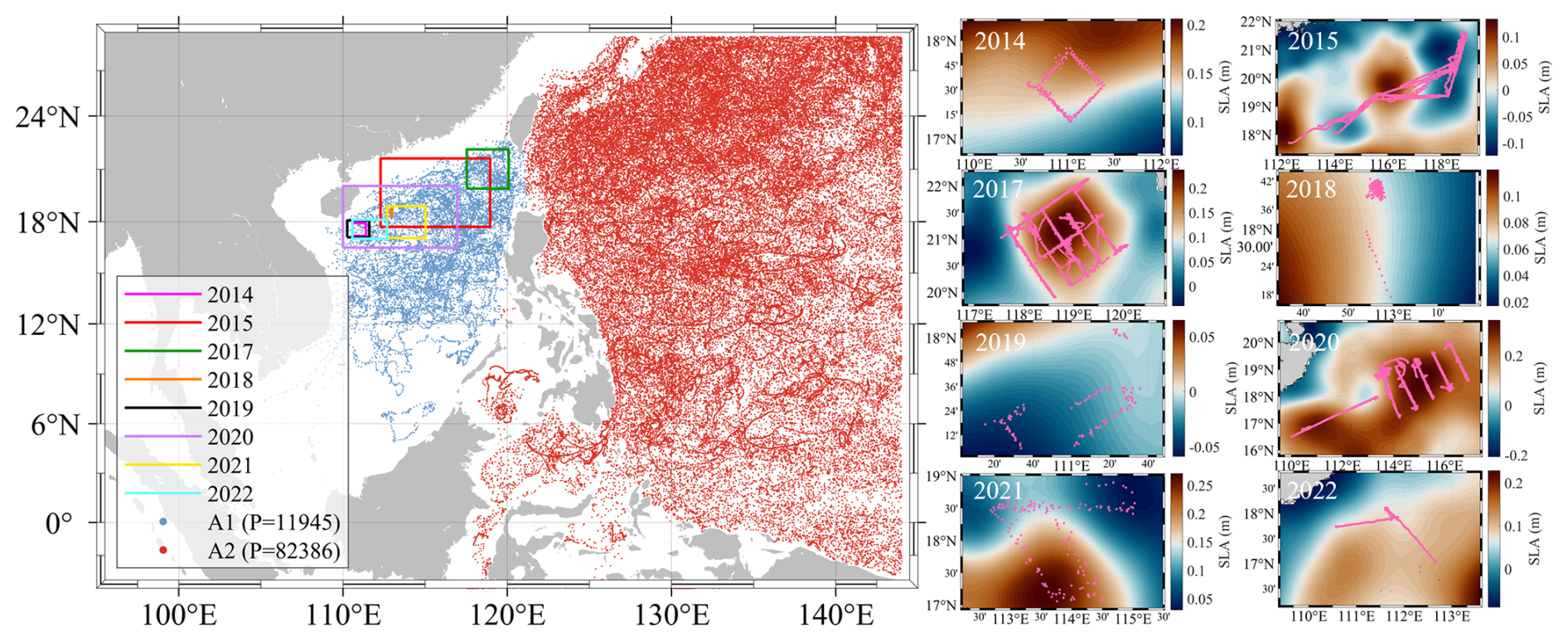
Figure 1Spatial distribution of ARGO profiles and SLA fields along UG tracks in the SCS and adjacent regions for eight years (2014, 2015, 2017, 2018, 2019, 2020, 2021, 2022). The left panel shows the locations of ARGO profiles. The right panels display SLA (in meters) during the UG observation periods for each year, with the corresponding UG tracks overlaid in pink.
The SLA data assimilated into SCSOFSv2 are the along-track SLA observations from multiple altimeter satellites distributed by AVISO of the Centre National D'études Spatiales (CNES), including the Jason-1/2/3, TOPEX/Poseidon, Sentinel-6 series and so on (Taburet et al., 2019). The along-track SLA data have been processed with standard geophysical corrections, including dry and wet tropospheric delay, ionospheric delay, solid Earth tide, polar tide, and sea state bias corrections. The data are available at https://www.aviso.altimetry.fr/en/home.html (last access: 2 December 2025).
The in-situ temperature–salinity profiles assimilated into SCSOFSv2 are obtained from Argo profiling floats of the International Argo Program, providing vertical profiles of temperature and salinity over the depth range of 0–2000 m (Argo Science Team, 1998; Roemmich et al., 2009). Argo data are downloaded from the Global Data Assembly Centre (GDAC) and subjected to quality control flag screening, retaining only profiles for which both temperature and salinity quality flags equal 1 (good), thereby excluding outliers and suspicious profiles. Prior to assimilation, Argo temperature–salinity profiles are vertically interpolated onto the standard depth levels corresponding to the original σ-coordinate system of the SCSOFSv2. Over the study period of 2001–2024, a total of 94331 Argo profiles were obtained, of which approximately 12 % were located within the A1 domain (Fig. 1). Argo temperature–salinity profiles are also used in the validation presented in this study. It is worth noting that although Argo data are assimilated into the system, the profiles are first interpolated onto the standard vertical depth levels corresponding to the model σ-coordinate system prior to assimilation, resulting in a loss of sampling detail from the original depth levels. During validation, the model temperature–salinity analysis fields are interpolated onto the original measured depths of each Argo float, and pointwise biases are computed at the non-uniform native sampling depths of the Argo profiles. The root mean square error (RMSE) and bias are then calculated after interpolation, providing an assessment of the ability of SCSORA to reproduce the subsurface thermohaline vertical structure. The Argo data are available at https://argo.ucsd.edu/data/ (last access: 12 December 2025).
For SST validation, the present study employs the Operational Sea Surface Temperature and Sea Ice Analysis (OSTIA) product distributed by the UK Met Office, which provides daily mean blended SST data at a horizontal resolution of ° (Donlon et al., 2012). OSTIA integrates multisource satellite infrared and microwave SST observations together with in-situ measurements, generating a gap-free global SST analysis field via optimum interpolation. Given the differences between OSTIA and OISST products in data sources, blending algorithms, and spatial resolution, OSTIA serves as a suitable reference dataset for SST accuracy assessment. The OSTIA product is available at https://doi.org/10.48670/moi-00168 (Copernicus Marine Service, 2024b).
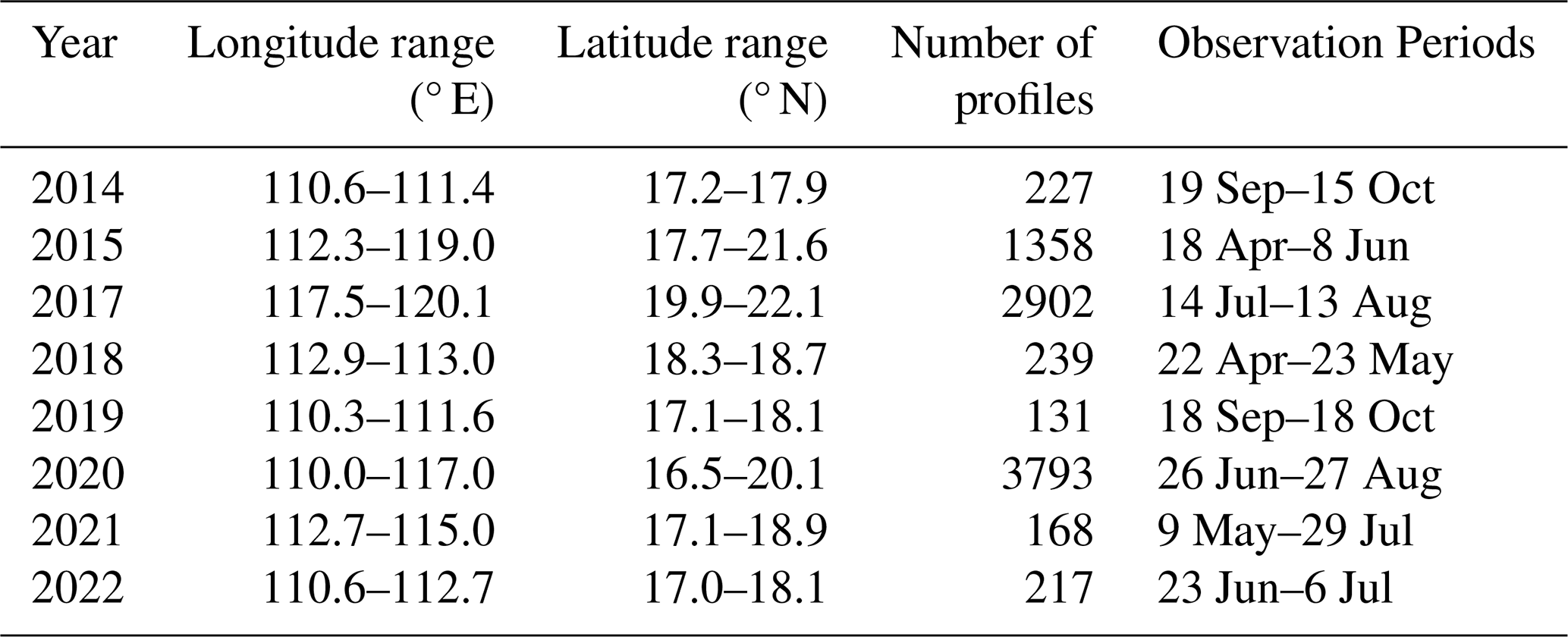
To further evaluate the capability of the SCSORA in reproducing subsurface thermohaline structure in the eddy-active region of the northern South China Sea (NSCS), the present study incorporates the high-resolution underwater glider (UG) temperature–salinity observation dataset publicly released by Qiu et al. (2025a). This dataset is based on multiple dedicated observation campaigns targeting mesoscale eddies and submesoscale processes in the SCS and is available at https://doi.org/10.57760/sciencedb.11996 (Qiu et al., 2025b). The validation period spans 2014–2022, with observations concentrated in the eddy-active region of the NSCS; details are provided in Table 1. Across eight cruises, a total of 9035 temperature–salinity profiles are available, encompassing spring (April–June), summer (July–August), and autumn (September–October) seasons, enabling characterization of the seasonal thermohaline vertical structure in the eddy-active region of the NSCS. Since the UG data are not incorporated into any assimilation procedure of SCSOFSv2, they serve as a rigorous independent benchmark for evaluating the subsurface thermohaline accuracy of the SCSORA in dynamically complex eddy regions. Their high spatial resolution enables detailed characterization of the thermohaline fine structure within eddies.
The SLA validation data are the multi-satellite merged gridded SLA product distributed by AVISO, with a horizontal resolution of ° and daily temporal resolution. This merged gridded product is generated by fusing along-track observations from multiple altimeters via optimum interpolation and is independent of the raw along-track SLA data assimilated by SCSOFSv2 at the data processing level, making it suitable for assessing the SLA accuracy of the SCSORA and the spatial reproducibility of mesoscale eddy signals. The data are available at https://doi.org/10.48670/moi-00148 (Copernicus Marine Service, 2024a).
Surface current observations were obtained from the Global Drifter Program (GDP), which is maintained by the National Oceanic and Atmospheric Administration (NOAA) and provides one of the most extensive in-situ datasets of near-surface currents worldwide (Lumpkin and Pazos, 2007). The GDP drifters are drogued at 15 m depth, so their trajectories primarily reflect the near-surface flow at that level rather than the instantaneous skin-layer current, thereby substantially reducing the direct wind-driven drift effect on the buoy motion (Niiler, 2001; Lumpkin et al., 2017). Drifter positions are typically reported at hourly intervals and are quality-controlled, with the effects of wind slip and drogue loss flagged and, where appropriate, corrected (Lumpkin et al., 2017; Elipot et al., 2016). In this study, drifter data spanning 2001–2024 in the SCS were used. The 6-hourly interpolated product was employed, and velocity estimates were derived from finite differences of successive positions. Only data flagged as good quality and with drogues confirmed to be present were retained, yielding a total of 174 696 valid samples. It should be noted that individual drifter trajectories are Lagrangian and may be influenced by submesoscale processes, Stokes drift, and residual wind slip, which should be taken into account when interpreting the comparison with the Eulerian model output.
2.3 Methods
2.3.1 Statistical tests
The performance of the model was assessed using various statistical metrics, such as the RMSE, correlation coefficient (R2), and Bias. The following formulas were used:
where xi is the observed value of pixel i, yi is the SCSORA analysed value of pixel i, and is the average of all true values.
2.3.2 MHW Statistical Method
MHW characteristics are identified following the definition of Hobday et al. (2016), whereby a MHW event is defined as a discrete period during which daily SST exceeds the climatological 90th percentile threshold for at least five consecutive days; two successive events separated by a gap of no more than two days are treated as a single continuous event. The annual 90th percentile threshold and climatological SST for date i are computed by pooling all daily SST values within an 11 d window centred on date i (i.e., days i−5 to i+5) across all years of the 2001–2024 baseline period, followed by smoothing with a 31 d moving average window. The code used to compute MHW metrics is obtained from https://github.com/ZijieZhaoMMHW/m_mhw1.0 (last access: 20 March 2026, (Zhao and Marin, 2019).
2.3.3 Eddy Detection Method
Mesoscale eddies in the SCS are identified and tracked using the Eulerian vector geometry-based automatic eddy detection method of Nencioli et al. (2010). This Eulerian vector geometry approach is characterized by a high successful detection rate (SDR) and a lower excessive detection rate (EDR) compared with alternative methods and has been extensively validated across multiple ocean regions including the SCS, the Bay of Bengal, the subtropical counter current zone, the Gulf Stream, the North Pacific Ocean, and the Southern Ocean (Nencioli et al., 2010; Sun et al., 2019; An et al., 2022). The eddy identification and tracking procedure comprises three sequential steps: determination of eddy centers, delineation of eddy boundaries, and reconstruction of eddy trajectories. Eddy center detection requires the simultaneous satisfaction of four geometric constraints (Nencioli et al., 2010); in the present study, the parameters are set to A = 3 and B = 2, respectively. The eddy boundary is defined as the outermost closed streamline surrounding the eddy center, the eddy radius is defined as the mean distance from the boundary points to the eddy center, and eddy trajectories are determined by matching eddy center positions between successive time steps.
3.1 SST Validation Using Satellite Datasets
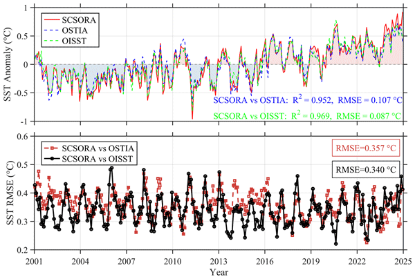
SCSORA reproduces SST trend patterns that are consistent with those of the satellite-based analysis products OSTIA and OISST (Fig. 2). The three datasets exhibit highly coherent variations in SST anomalies. SST in the study region exhibits a pronounced warming trend, with the warming signal becoming increasingly evident after 2016 and reaching the highest positive anomaly levels of the entire study period by 2024. On interannual timescales, SST anomalies display a distinct alternating pattern of cold and warm phases, with negative anomalies predominantly concentrated around 2001–2010 and positive anomalies emerging during periods such as 2016–2024, indicating a significant warming trend. Furthermore, SCSORA accurately captures key interannual variability signals observed in both OSTIA and OISST, including the pronounced warm anomaly associated with the strong El Niño event of 2009–2010 (Kim et al., 2011) and the marked warming episode during 2023–2024 driven by the combined effects of a sustained long-term warming trend and the re-emergence of large-scale ocean–atmosphere anomalies (Cheng et al., 2024a; Terhaar et al., 2025). The RMSE of SST remains stable over the entire study period. Specifically, the mean RMSE is 0.357 °C between SCSORA and OSTIA, and 0.340 °C between SCSORA and OISST. These results indicate the high stability of the model and demonstrate that SCSORA can effectively reproduce both the short-term variability and the long-term trend of SST.
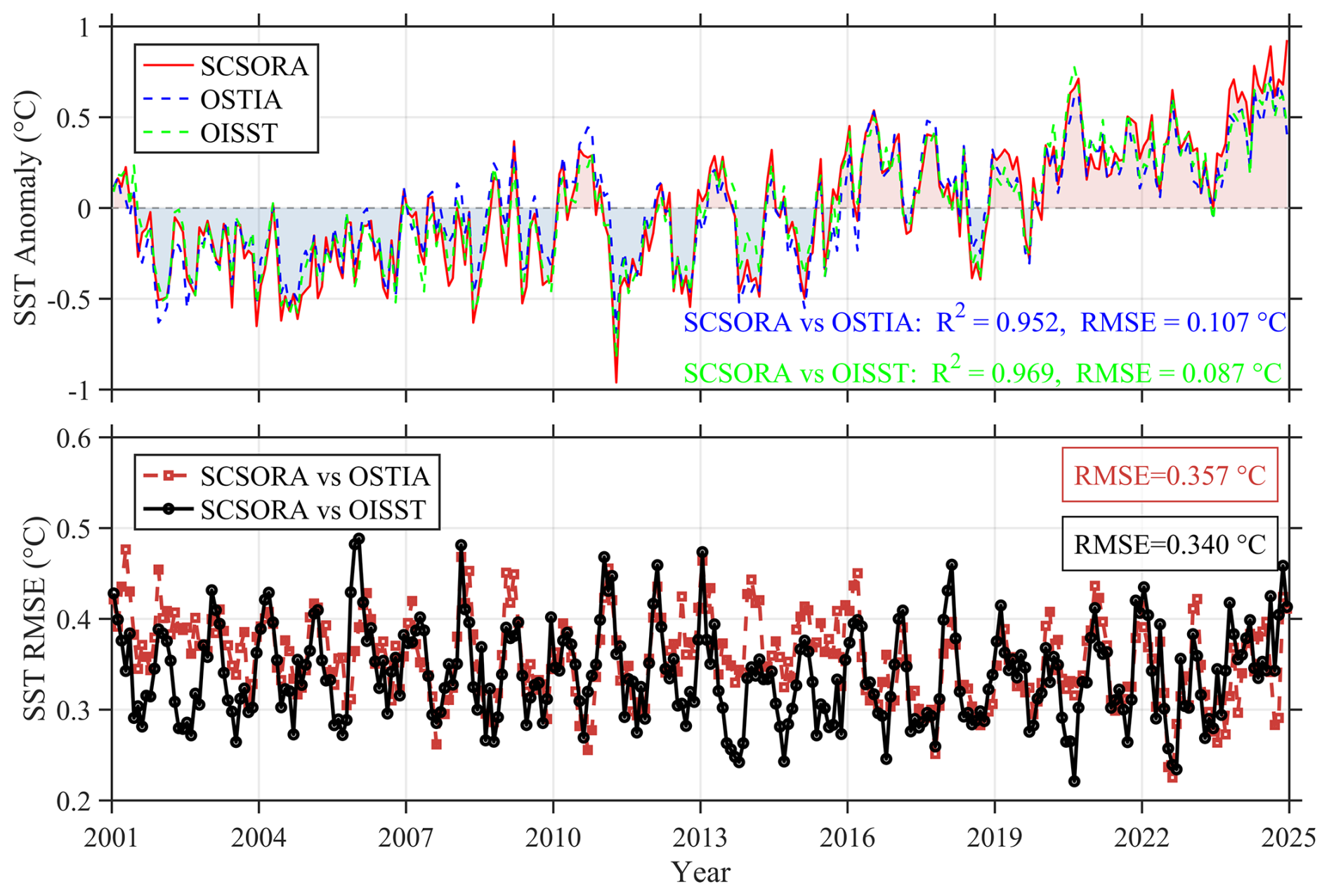
Figure 2Time series of SST anomalies and RMSE relative to the 2001–2024 SST climatology. Comparisons are shown among SCSORA, OSTIA, and OISST. SST anomalies are computed as daily departures from the 2001–2024 climatological SST.
The RMSE of SST between SCSORA and both OISST and OSTIA exhibits pronounced regional disparities and seasonal evolution (Fig. 3). Overall, the RMSE in the central open waters of the SCS is generally below 0.5 °C, whereas larger errors are predominantly distributed in the Taiwan Strait, the northern SCS continental shelf, and certain coastal regions, with localized values exceeding 0.8 °C. Such spatial discrepancies may be associated with complex ocean dynamical processes in nearshore and shelf seas, such as monsoon-driven coastal circulations, tidal mixing, and local upwelling.
In terms of seasonal variability, the RMSE increases markedly during winter in the northern SCS and adjacent to the Taiwan Strait, forming a relatively prominent high-error region. Previous studies have demonstrated that the northeasterly monsoon can drive the southward transport of cold coastal water and generate a distinct SST front in the Taiwan Strait; concurrently, intensified wintertime sea surface cooling in the northern SCS further enhances the regional temperature gradient (Kuo et al., 2018). Therefore, the relatively large RMSE in these regions may be attributed to model biases in simulating monsoon-driven sea surface heat fluxes, coastal water mass transport, and the positioning of temperature fronts. As the northeasterly monsoon gradually weakens, the high-error extent in the northern SCS diminishes accordingly. During summer, the central open waters of the SCS maintain relatively low RMSE, yet a localized high-value band emerges along the Vietnam coast. Xie et al. (2003) noted that the southwesterly monsoon can drive coastal upwelling off Vietnam and promote the offshore expansion of cold water through local wind stress curl and anticyclonic circulation. These processes may intensify the local SST spatial gradient, rendering the simulated results in this region more sensitive to the accuracy of wind fields, vertical mixing, and horizontal advection. Nevertheless, SCSORA is capable of reproducing SST over most of the SCS reasonably well across all seasons, particularly exhibiting low RMSE in open waters, which indicates its favorable capability for SST reconstruction.
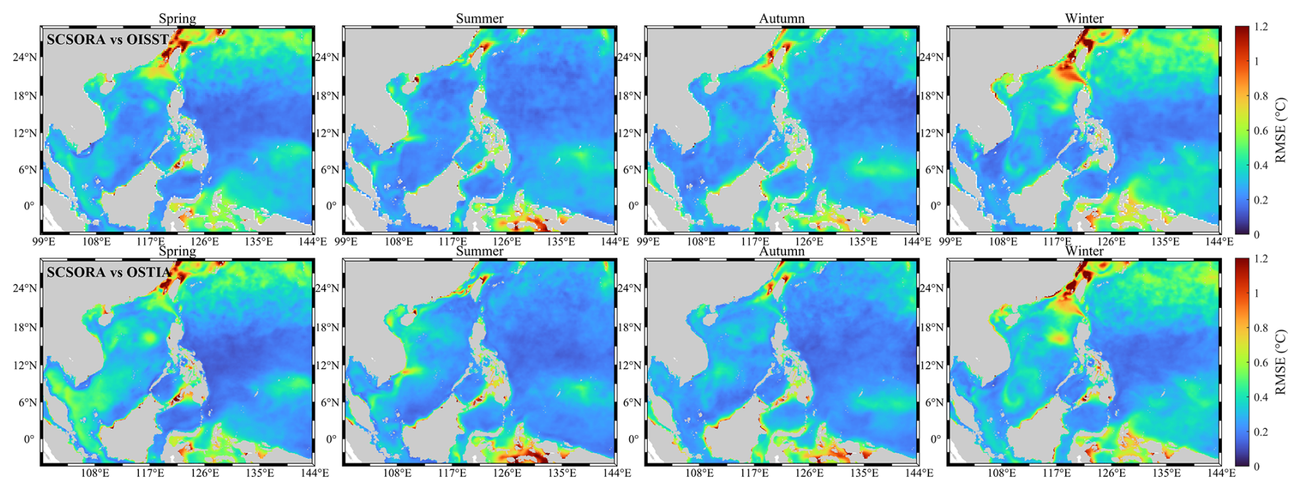
Figure 3Seasonal spatial distributions of SST RMSE between SCSORA and OISST (top row) and between SCSORA and OSTIA (bottom row) for spring, summer, autumn, and winter (from left to right).
3.2 SLA Validation based on AVISO
The AVISO multi-source satellite merged gridded product (AVISO_G) represents an important reference dataset for SLA research and has been widely adopted in ocean model validation studies (Juhl et al., 2025; Kerry et al., 2024). SCSORA successfully captures the low-frequency variability of SLA over the period 2001–2024, exhibiting a high degree of agreement with the AVISO_G SLA product in terms of large-scale trends and interannual variability, with both datasets clearly exhibiting consistent multi-year oscillatory characteristics (Fig. 4). In particular, the significant negative anomaly signals associated with La Niña events around 2010 and following 2016 are consistently reproduced in both datasets, demonstrating the reliability of SCSORA in capturing variability on interannual and longer timescales. The RMSE of SLA between the two datasets is generally maintained within the range of 4.5–9.7 cm and a mean value of 5.9 cm. The temporal stability of the error throughout the whole period indicates consistent and sustained model performance, confirming that SCSORA is capable of reproducing large-scale sea surface anomaly patterns with reasonable accuracy.
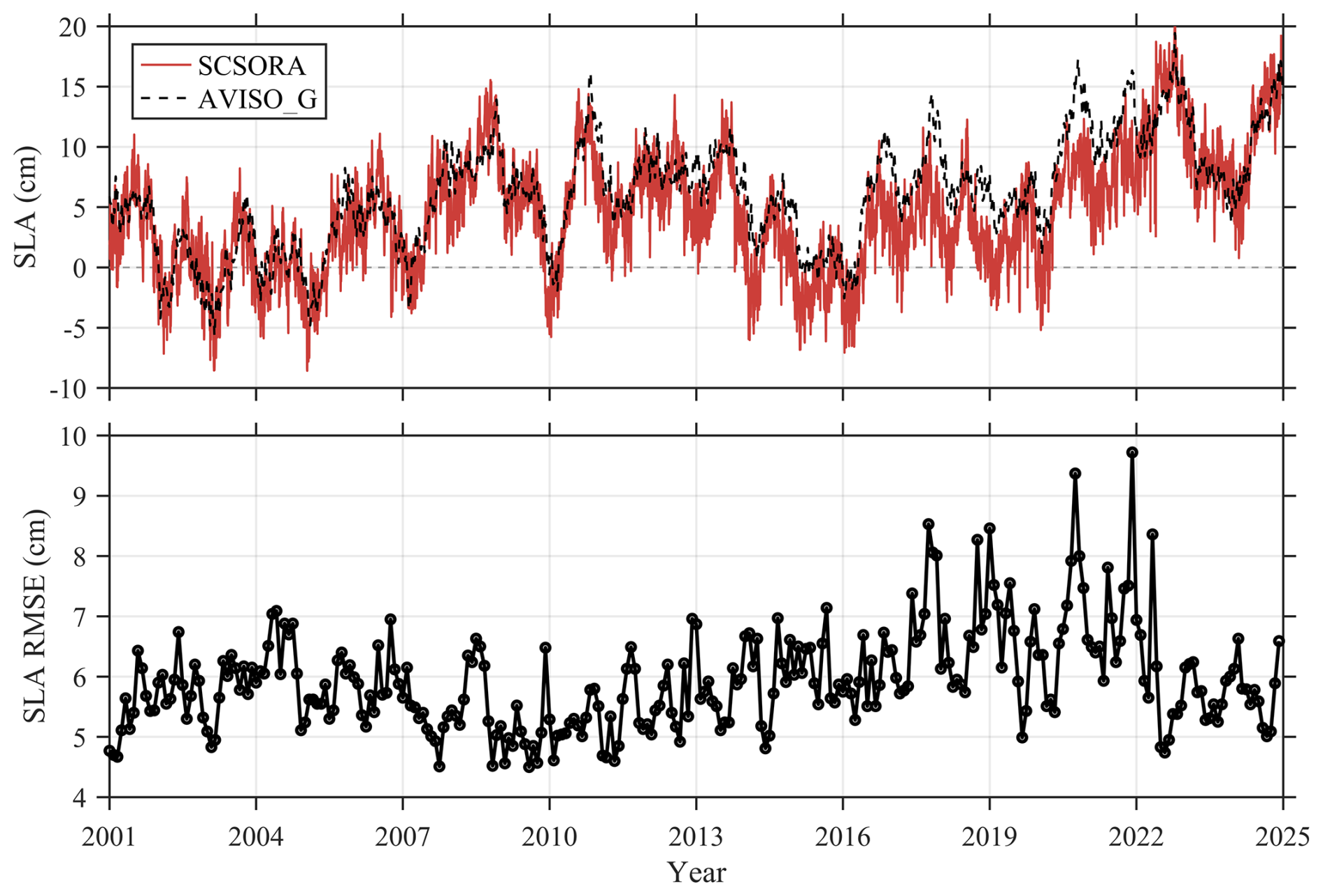
Figure 4Time series of SLA and RMSE between the SCSORA and AVISO observations. RMSE represents the temporal deviation of the SCSORA from the observations over the same period.
The RMSE of SLA between SCSORA and both along-track (AVISO_T) and gridded (AVISO_G) AVISO products exhibits pronounced spatial disparities and seasonal variability (Fig. 5). The RMSE is relatively low in the central and southern open waters of the SCS, with values below 5 cm over most of the region, whereas larger errors are primarily distributed in the Luzon Strait, the vicinity of Taiwan and the northwestern Pacific to the east thereof, where localized values exceed 10 cm. These regions also exhibit relatively higher errors across different seasons. These areas are significantly influenced by the Kuroshio and mesoscale eddy activities, characterized by strong SSH variability (Nan et al., 2015). Therefore, the relatively large RMSE may be attributed to model biases in simulating Kuroshio path variability, eddy activity, and the associated SSH gradients. Nevertheless, in general, SCSORA exhibits relatively low RMSE against both AVISO datasets over most of the open waters of the SCS, although considerable discrepancies remain in regions with intense Kuroshio and mesoscale eddy activity.
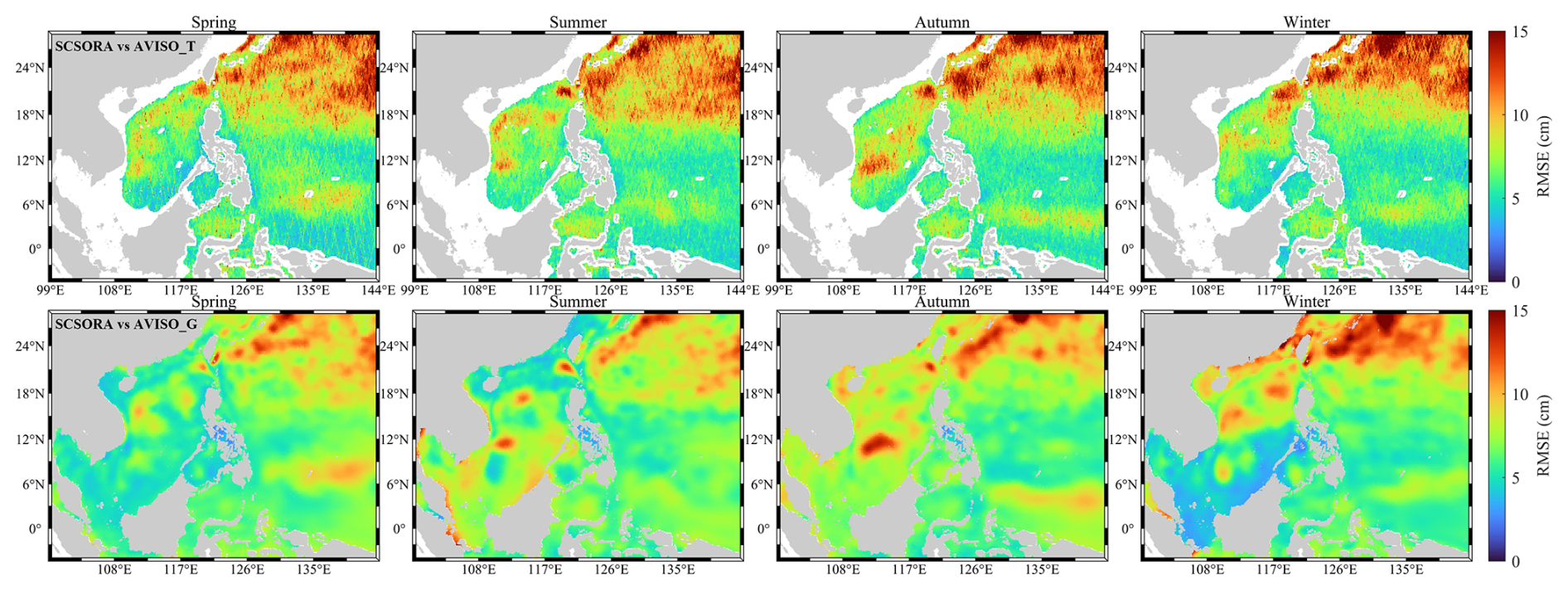
Figure 5Seasonal spatial distributions of SLA root mean square error (RMSE) between SCSORA and AVISO_T data (top row) and AVISO_G data (bottom row) for spring, summer, autumn, and winter (from left to right).
3.3 Temperature/Salinity Validation Using In-Situ Observations
SCSORA shows generally well agreement with Argo float temperature–salinity profiles (Fig. 6). Based on more than 10.9 ×10⁶ matched temperature samples, the validation results indicate a regression slope of 1.00, an R2 of 0.99, and an RMSE of 0.56 °C, demonstrating a high level of consistency between the SCSORA and observations throughout the entire water column. The corresponding statistics for salinity are a slope of 0.91, a R2 of 0.91, and a RMSE of 0.06 PSU, respectively. The vertical bias distribution shows that temperature biases remain close to zero over most depth ranges, while relatively large variability is observed in the upper 200 m, likely associated with seasonal thermocline variability. A slight warm bias is present near the main thermocline at 200–600 m depth. For salinity, a negative bias is observed in the near-surface layer. Below 800 m, both temperature and salinity biases approach zero, and the spread decreases substantially.
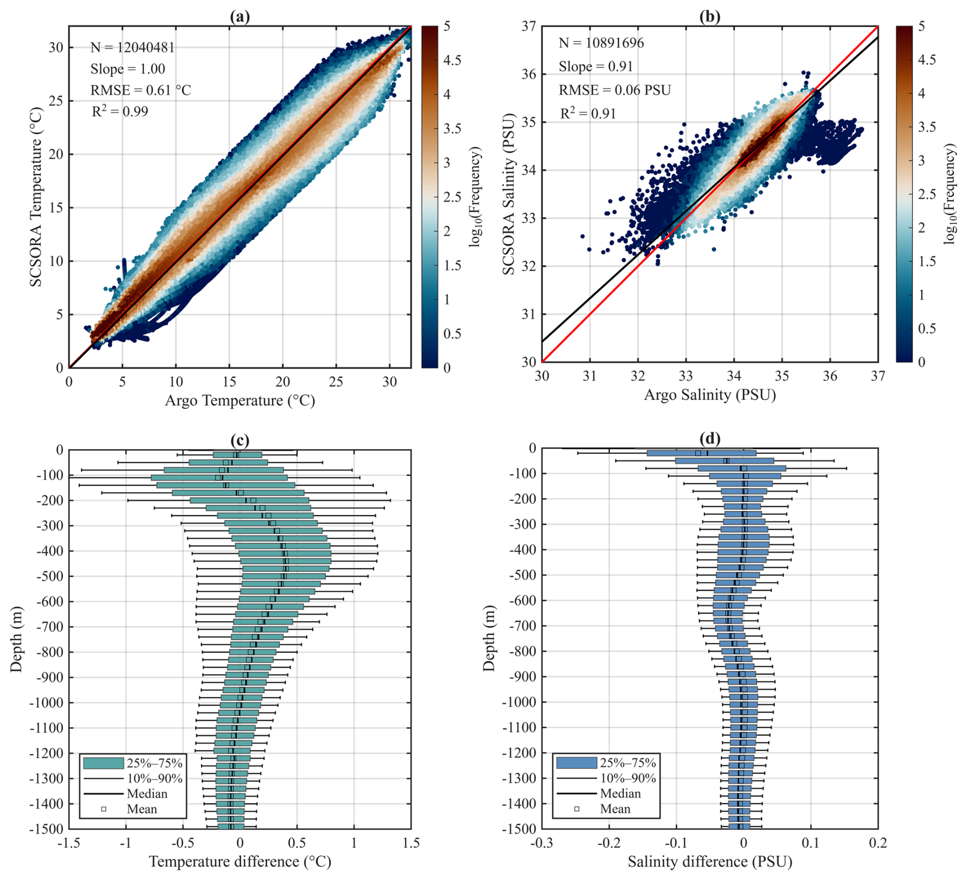
Figure 6Comparison between SCSORA and ARGO observations. Panels (a) and (b) show scatter plots of temperature (T) and salinity (S) at observation points, with the 1:1 line indicated. The sample size is denoted by N. Panels (c) and (d) display the vertical distribution of analysis–observation differences (SCSORA minus ARGO) for temperature and salinity, illustrating the depth-dependent bias in the model.
Based on UG observations from eight independent years (2014, 2015, 2017, 2018, 2019, 2020, 2021, and 2022), covering the depth range from the sea surface to 1000 m, the comparison indicates that the temperature differences between the SCSORA and the UG observations are generally small across all years. The mean biases throughout most of the water column remain within ±1.5 °C, although in some years relatively large temperature differences occur at depths of approximately 100–400 m, with local mean biases approaching 2 °C (e.g., in 2014; Fig. 7). Relatively elevated spread is present in the surface layer of SCSORA, yet errors remain within 1.5 °C throughout. Below 200 m, the interquartile range (25th–75th percentile) narrows substantially, indicating more stable model performance in the intermediate and deep layers. The salinity differences exhibit a depth-dependent structure similar to that of temperature: bias spread is larger in the upper and decreases progressively with depth. Across the eight years, mean salinity biases below 400 m are generally close to zero, suggesting that SCSORA is capable of reproducing the halocline structures with reasonable fidelity. Overall, SCSORA shows satisfactory agreement with the UG observations, particularly in the subsurface and deeper layers, indicating that the model can reliably reproduce subsurface thermohaline structures within the regions and periods sampled by the UG.
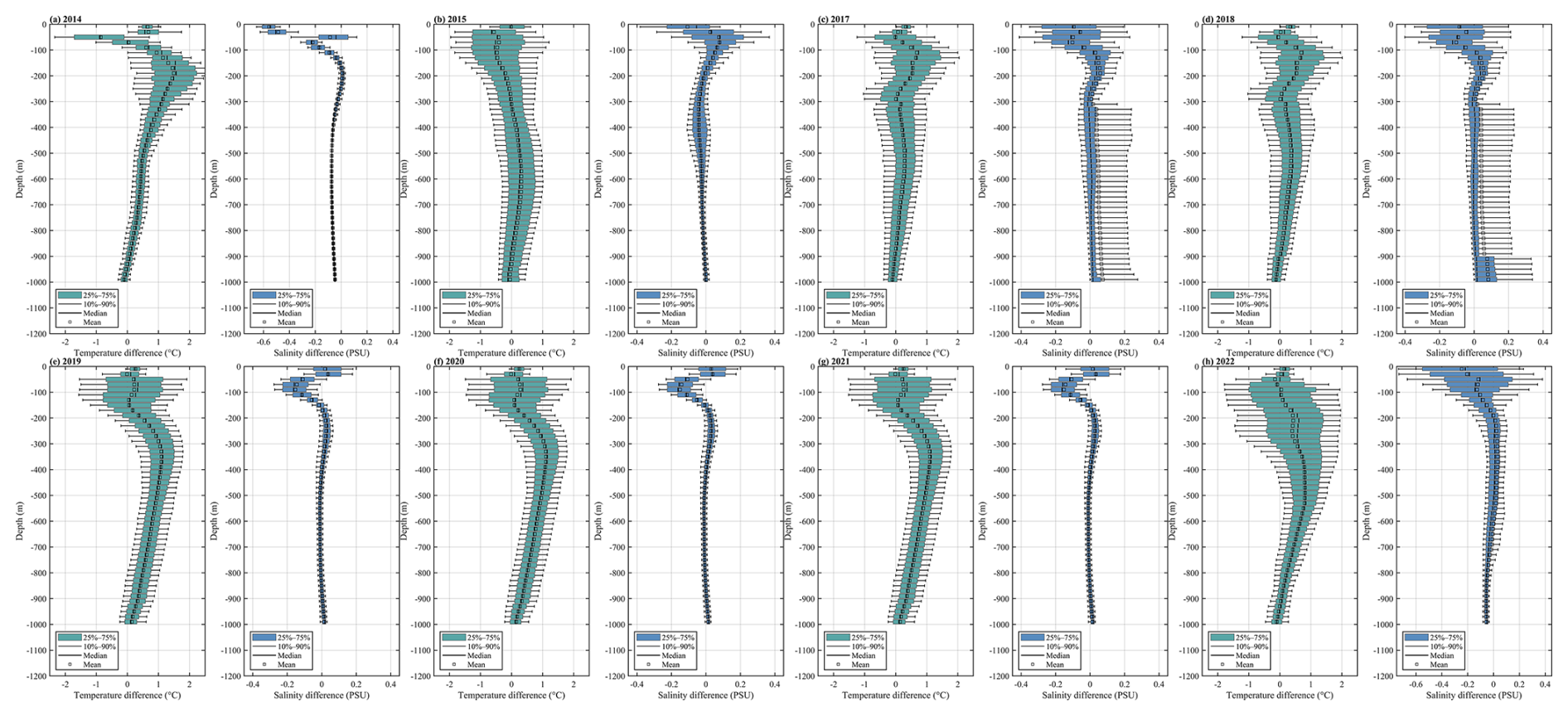
Figure 7Vertical distribution of temperature (T) and salinity (S) differences between SCSORA and UG observations for each year. Each panel corresponds to a specific year, showing the model minus observed values, highlighting the depth-dependent bias of the model relative to the UG measurements.
SCSORA is capable of reproducing the temperature and salinity distribution characteristics along the UG observational sections reasonably well (Fig. 8). In terms of temperature, SCSORA is generally consistent with the observed thermocline position and major vertical gradients in most years. The surface temperature is approximately 28–30 °C, with a pronounced temperature decrease within the depth range of roughly 50–200 m. Combined with the temperature bias statistics, the mean temperature bias within most of the water column is constrained to within ±1.5 °C, with the error dispersion generally decreasing below 200 m, indicating that SCSORA exhibits favourable stability in reproducing subsurface temperature structure. With respect to salinity, both datasets display relatively comparable vertical distributions across most observational depths, with salinity ranging from 34 to 35 PSU. Compared with temperature, salinity discrepancies are generally smaller, and the errors diminish with increasing depth. Below 300 m, the salinity structure exhibits high consistency in most years; however, the dispersion in the upper ocean is relatively larger, with localized salinity overestimation occurring in certain years (e.g., 2014, 2020, 2022). It should be noted that the SCSORA data are daily-averaged products, which are inherently smoother than the UG observations; consequently, the localized vertical undulations within the thermocline and upper ocean, as well as short-timescale temperature and salinity anomalies present in the observations, are markedly attenuated in SCSORA. This phenomenon is associated with the smoothing of high-frequency signals induced by daily averaging and tidal mixing missed in SCSOFSv2.
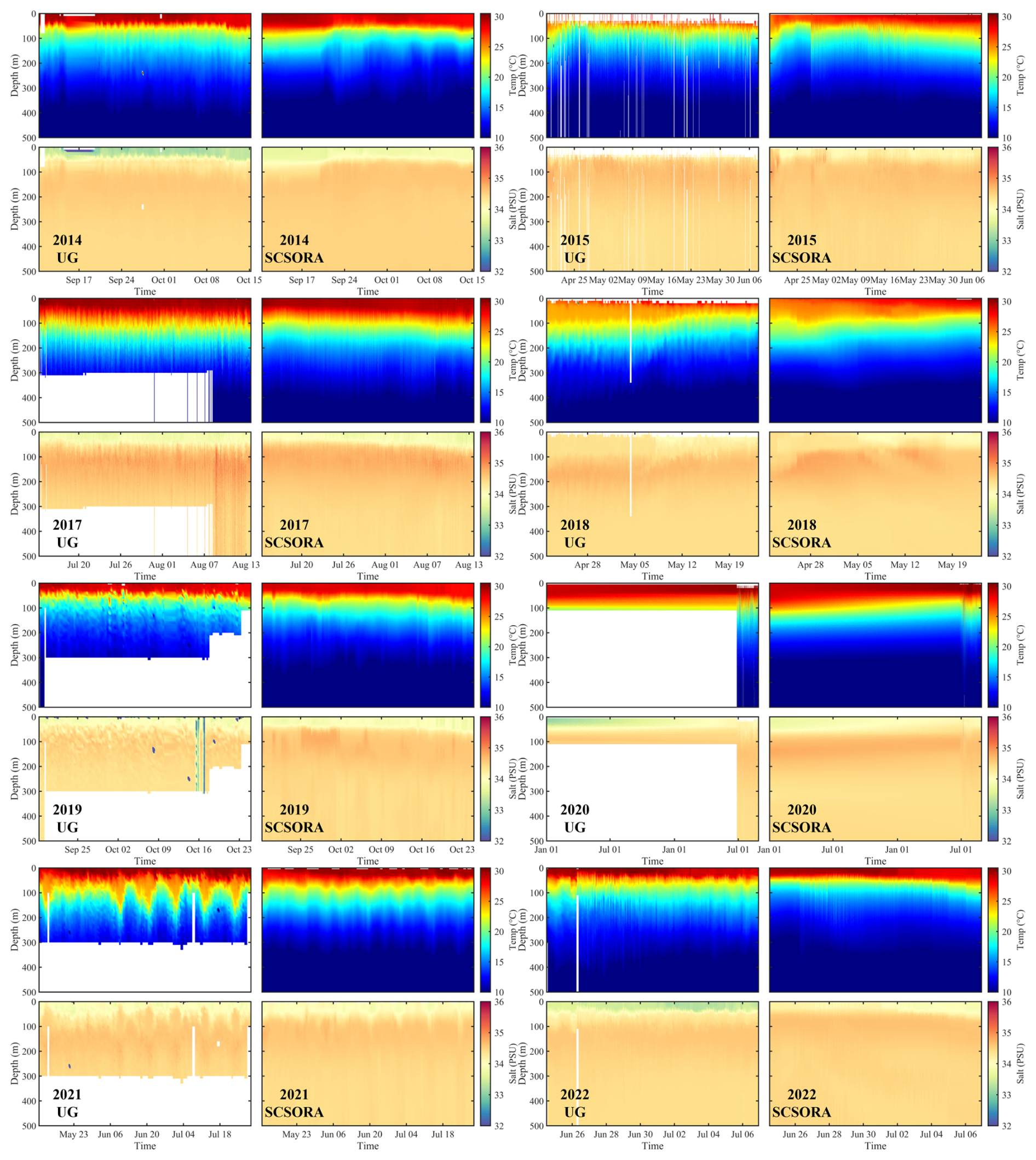
Figure 8Comparison of vertical section time series of temperature (upper panels) and salinity (lower panels) between UG observations (left column) and SCSORA simulations (right column) from 2014 to 2022.
3.4 Mixed layer depth
Climatological MLD is computed separately for the four seasons: spring, summer, autumn, and winter (Fig. 9). Calculations of MLD are performed for SCSORA (left column) and GLORYS (middle column) using the standard criterion of a temperature difference threshold of ΔT = 0.2 °C relative to the 10 m reference depth (Cheng et al., 2024b). Both SCSORA and GLORYS exhibit good consistency in the spatial distribution of MLD across all four seasons, capturing the principal seasonal variability and regional contrasts between the deep SCS basin and the surrounding shelf and coastal regions.
In spring, both products simulate relatively shallow MLD over most of the SCS (approximately 10–30 m), while deeper mixed layers exceeding 40 m appear in the central western Pacific region. The zonal mean profiles are in closed agreement throughout the domain, with a mean absolute error (MAE) of 3.5 m, indicating overall good consistency despite localized differences in the intensity of the deep mixed layer near 24° N.
In summer, under the strong stratification driven by solar heating, MLD shoals markedly in the northern western Pacific Ocean, with mean MLD maintained within 20–40 m across most latitude bands in both SCSORA and GLORYS. Agreement between the two datasets is the highest in this season, with a MAE of 3.0 m, demonstrating that SCSORA adequately reproduces the dominant physical mechanisms governing summer stratification. Nevertheless, both datasets exhibit MLD deepening in the southern part of the domain, which may be associated with enhanced vertical mixing driven by intensified southwest monsoon wind stress, precipitation effects, and salinity gradient changes (Thompson and Tkalich, 2014; Sallée et al., 2021; Chen et al., 2023). In addition, oceanic current dynamics and coastal upwelling may contribute to mixed layer deepening in the southern domain, producing a trend opposite to that observed in the northern region.
In autumn, the Asian monsoon system transitions gradually from the summer southwest monsoon to the winter northeast monsoon (Wang et al., 2009). As surface cooling intensifies and monsoon wind stress increases, MLD deepens again in the NSCS and the adjacent western Pacific Ocean, a seasonal evolution that is reasonably well reproduced by both products. The zonal mean profiles from the two products are broadly consistent in structure, with MLD of SCSORA simulating slightly shallower than that of GLORYS; the MAE is 2.0 m, indicating that SCSORA captures the physical characteristics of mixed layer deepening in this season.
In winter, it exhibits the most pronounced seasonal MLD signal of the year, closely associated with the vigorous winter monsoon forcing and substantial net heat loss at the ocean surface. Over the SCS and the adjacent northwestern Pacific Ocean, the winter northeast monsoon is accompanied by cold air intrusions and atmospheric cooling. These conditions enhance negative buoyancy flux and wind stress-driven mixing at the sea surface, leading to significant mixed layer deepening (Thompson and Tkalich, 2014; Thoppil, 2023). Both products simulate pronounced winter mixed layer deepening in the NSCS and the western Pacific region, consistent with the wintertime convective mixing process under monsoon forcing. The zonal mean profiles in winter also display the largest MLD values of the annual cycle, reaching up to 80 m north of 18° N, reflecting the basin-scale response to intense mixing driven by the winter northeast monsoon. The mean MAE between the two datasets in winter is 3.0 m.
Overall, the MAE between SCSORA and GLORYS remains at a relatively low level of 2.0–3.5 m across all four seasons, demonstrating that SCSORA is capable of reliably reproducing the seasonal variability of MLD in the SCS and adjacent regions, with an accuracy comparable to that of the well-established GLORYS reanalysis product.
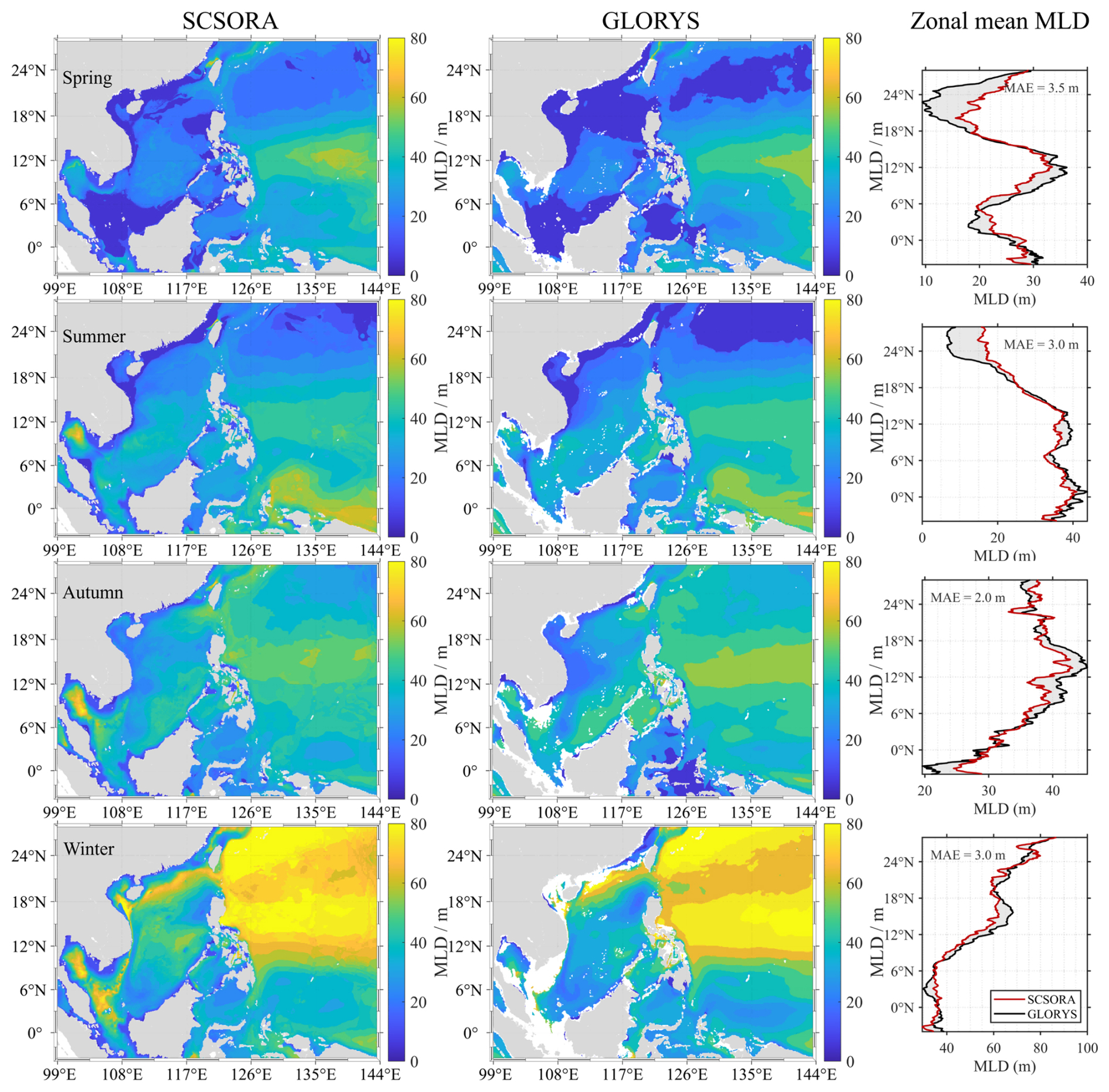
Figure 9Seasonal climatological MLD from SCSORA (left column) and GLORYS (middle column) for spring, summer, autumn, and winter, along with the corresponding zonal mean MLD profiles (right column; red: SCSORA, black: GLORYS). The MAE of zonal mean MLD between the two products is annotated in each right panel.
In addition, the annual mean bias between the MLD derived from UG and that from SCSORA was calculated (Fig. 10) to evaluate the capability of SCSORA in reconstructing the upper-ocean vertical mixing structure in the northern SCS. The results show that, except for 2014 when the bias is close to 0 m, the MLD simulated by SCSORA is generally deeper than that observed by the UG. Among these, the biases in 2017, 2018, and 2022 are the most pronounced, with mean biases of approximately −6.4, −6.1, and −6.9 m, respectively; the biases during 2019–2021 are relatively smaller, ranging from approximately −3.6 to −4.4 m. The interannual variability of the median bias is highly consistent with that of the mean bias.
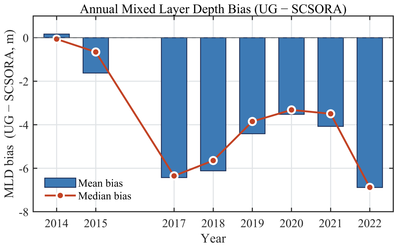
Figure 10Annual mean and median MLD bias between the UG observations and SCSORA (UG − SCSORA) from 2014 to 2022. Blue bars denote the annual mean bias, and the red line with dots denotes the annual median bias.
3.5 Current Validation Using Drifter Data
Since current observations are relatively scarce compared with temperature, salinity, and SLA, and surface velocity is readily influenced by wind-driven drift and mesoscale processes, we first conducted a qualitative validation of the surface current field through the spatial correspondence between representative GDP trajectories and the SCSORA surface current field and SLA. Figure 11 presents several typical GDP observational cases alongside the contemporaneous SCSORA-simulated surface current field and SLA distribution. Overall, the GDP trajectories show good consistency with the simulated flow direction and velocity variations, most trajectories evolving along the direction of the simulated current field and aligning with the corresponding SLA gradients and closed contour structures. In regions of intense mesoscale eddy activities, the GDP trajectories are able to reflect the rotational characteristics of eddies. In the Luzon Strait and its adjacent waters, both the GDP trajectories and the simulated current field exhibit strong flow structures, demonstrating that SCSORA possesses a certain capability in characterizing the Kuroshio intrusion and associated circulation features. It should be noted that localized offsets between trajectories and simulated flow directions still exist (Fig. 11c), which may be related to the wind drift effect on drifting buoys, spatiotemporal sampling differences between GDP and the model, and local small-scale processes.
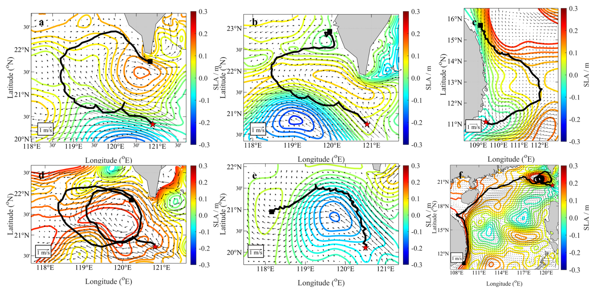
Figure 11Comparison between the SCSORA surface current field and drifting buoy trajectories. The thick black lines denote drifting buoy trajectories originating from the red stars; the arrows (units: m s−1) and contours (units: m) represent the SCSORA surface current field and SLA, respectively.
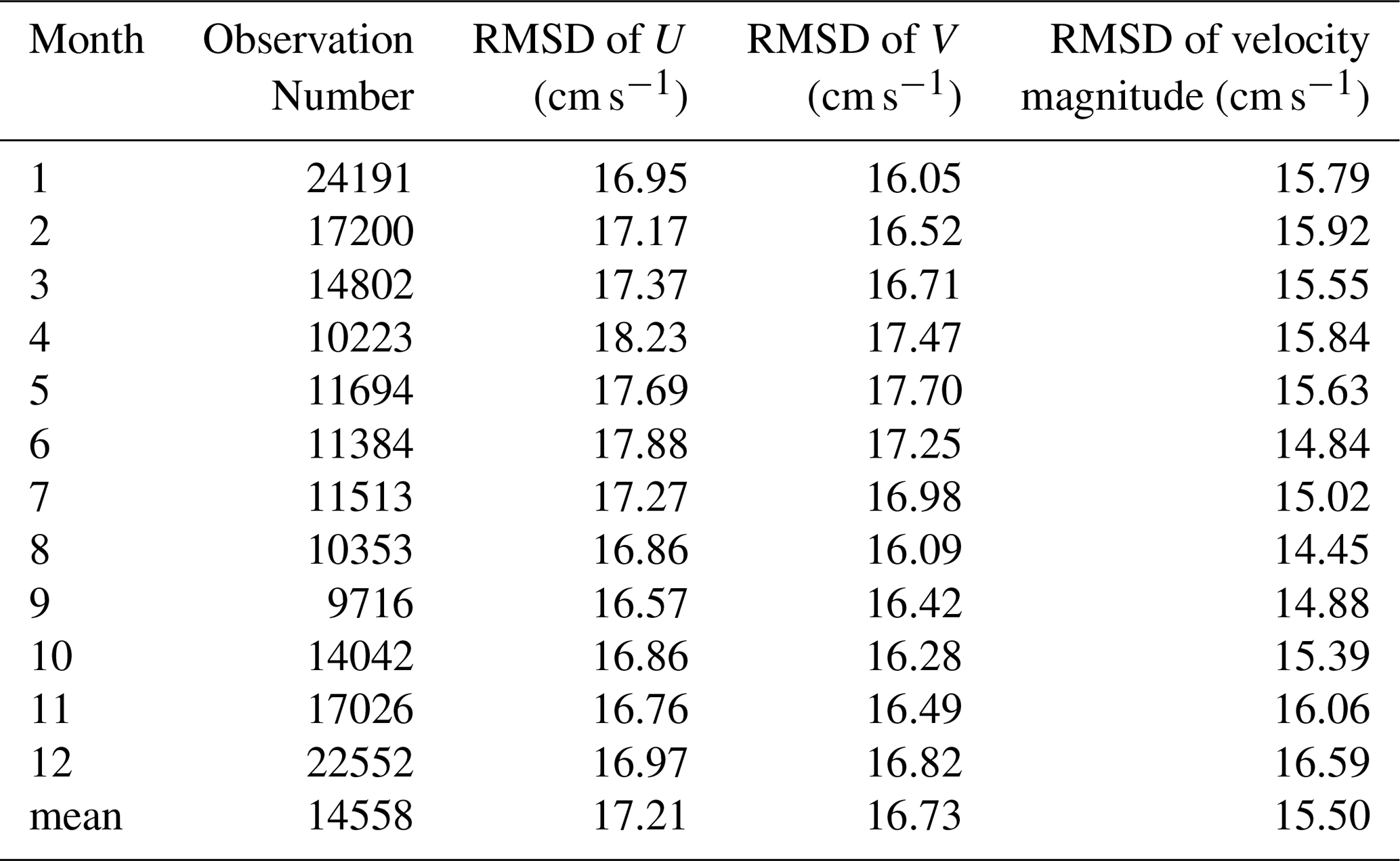
On this basis, a quantitative comparison of the SCSORA surface velocity was further conducted on a monthly basis using GDP data from the SCS for the period 2001–2024 (Table 2). A total of 174 696 valid GDP samples were obtained over the 24-year period. The monthly-scale root-mean-square differences (RMSD) calculated from contemporaneous samples over the 24 years indicates that the SCSORA surface velocity error is generally stable. The 12-month RMSD of the U component ranges from 16.57 to 18.23 cm s−1, with a mean of 17.21 cm s−1, being largest in April (18.23 cm s−1) and smallest in September (16.57 cm s−1); the RMSD of the V component ranges from 16.05 to 17.70 cm s−1, with a mean of 16.73 cm s−1, being largest in May (17.70 cm s−1) and smallest in January (16.05 cm s−1). The RMSD of the current speed ranges from 14.45 to 16.59 cm s−1, with a mean of 15.50 cm s−1, being smallest in August (14.45 cm s−1) and largest in December (16.59 cm s−1). The 12-month RMSD ranges of the three metrics are all relatively narrow, with the intermonthly ranges of the U component, V component, and current speed being 1.66, 1.65, and 2.14 cm s−1, respectively, indicating that the surface velocity error derived from the long-term sample statistics for 2001–2024 does not exhibit pronounced seasonal abrupt changes.
Overall, the mean RMSD of the SCSORA surface U component, V component, and current speed for 2001–2024 are 17.21, 16.73, and 15.50 cm s−1, respectively, with relatively limited error variation among different months. Combined with the consistency between the GDP trajectories and the simulated current field in terms of major circulation structures, SCSORA is able to reproduce the main spatial structure of the SCS surface current field and its seasonal variation characteristics reasonably. Meanwhile, the RMSD of approximately 15–17 cm s−1 also indicates that, although the model can adequately describe the major circulation and mesoscale structures, certain uncertainties remain in the precise characterization of the absolute magnitude of local current velocities. Therefore, the SCSORA surface current field can serve as a background flow field for studies of multi-scale ocean processes in the SCS; however, for applications highly sensitive to absolute velocity magnitudes, further evaluation in conjunction with independent observations or higher-resolution data is still warranted.
Table 2Climatological monthly root-mean-square differences between drifting buoy velocities and SCSORA velocities.
4.1 Spectral Energy Distribution
According to the validations in above, it is indicated that SCSORA is reliable and applicable in scientific research and operational contexts, SCSORA should be capable of reasonably reproducing the principal characteristics of the multiscale ocean dynamical processes, such as mesoscale eddies, MHW, upwelling, and oceanic fronts (Stammer, 1997, 1998; Bian et al., 2023). This section examines the potential of SCSORA in characterizing multi-scale dynamical processes from a spectral perspective, based on frequency–wavenumber power spectral analysis. The frequency–wavenumber power spectral density (PSD) of surface current velocity in the study area (Fig. 12) reveals that the spectral energy of all three products (SCSORA, GLORYS, and AVISO) is predominantly concentrated in the low-wavenumber, low-frequency domain ( cpkm, cph). This indicates that dynamical variability in this region is governed by mesoscale eddies and basin scale low-frequency seasonal to interannual processes (Ferrari and Wunsch, 2009; Schubert et al., 2020; Villas Bôas et al., 2022). With increasing wavenumber and frequency, spectral energy decays systematically across all three datasets, consistent with the general characteristic of oceanic turbulent spectra whereby energy diminishes with decreasing spatial scale. Nevertheless, pronounced differences exist among the three products in their capacity to resolve energy in frequency–wavenumber space.
SCSORA exhibits the broadest and most continuous spectral energy distribution among three products, with spectral energy extending to relatively high wavenumbers (approximately 10−1 cpkm) and frequencies (approximately 10−2 cph), displaying a smooth and gradual decay in the transition from the mesoscale to the submesoscale. SCSORA thus represents ocean dynamical processes over a broader range of spatiotemporal scales, and its approximately 4 km horizontal resolution gives it the potential to capture part of the submesoscale current variability. GLORYS exhibits a spectral distribution similar to that of SCSORA from low to moderate wavenumbers; however, its energy begins to decay markedly as wavenumbers approach 10−2 cpkm and a progressive spectral rolloff becomes evident, reflecting the limitation of its effective resolution in characterizing high-wavenumber processes. In contrast, AVISO has the most restricted spectral coverage, with its energy largely confined to wavenumbers below approximately cpkm. Consequently, the AVISO product primarily captures large-scale to mesoscale current variability and lacks the capability to resolve submesoscale processes due to its 25 km low horizontal resolution.
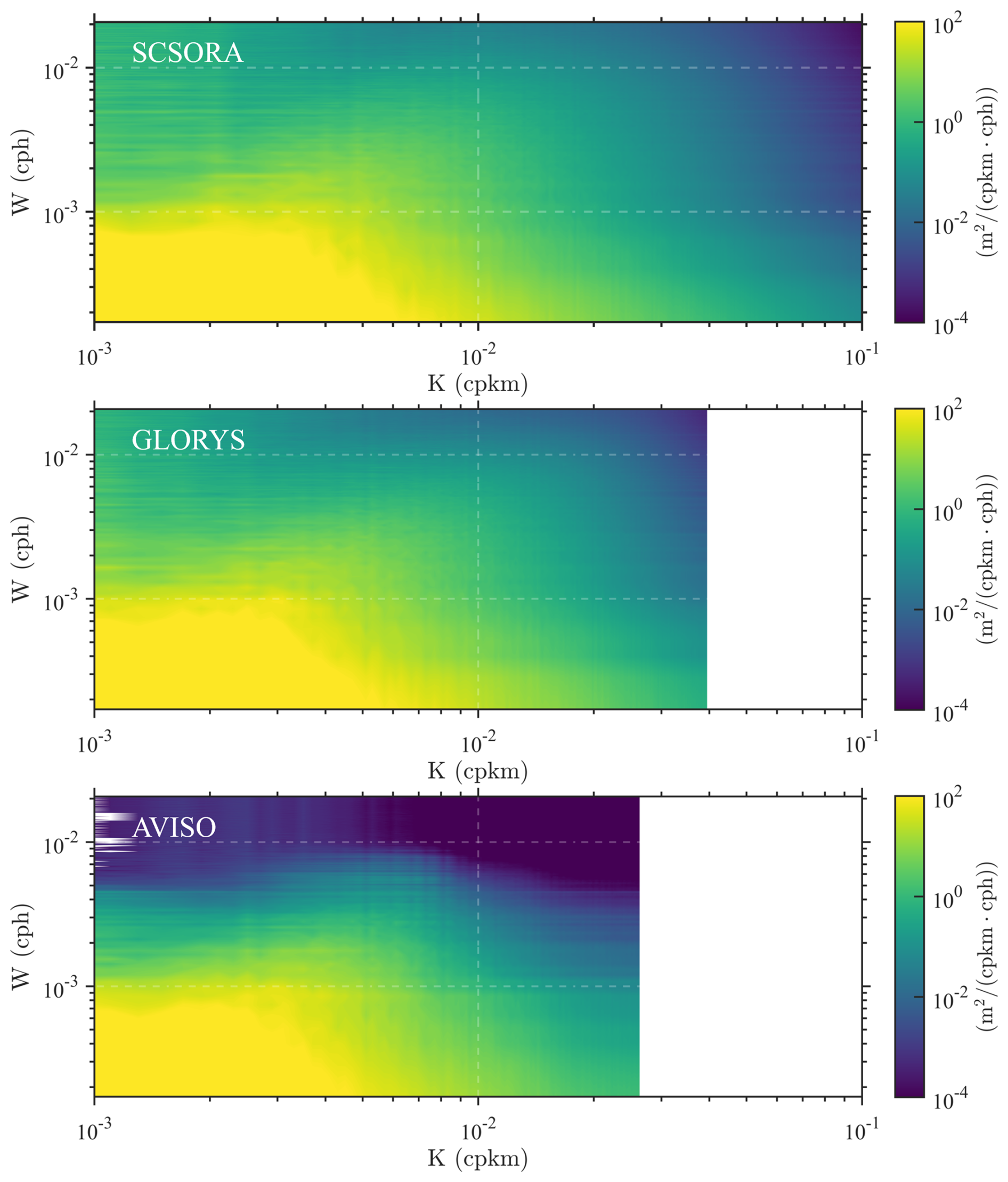
Figure 12Two-dimensional frequency-wavenumber power spectral density (PSD) of sea surface velocity from SCSORA (top), GLORYS (middle), and AVISO (bottom). The horizontal axis K denotes spatial wavenumber (cpkm, cycles per kilometer) and the vertical axis W denotes temporal frequency (cph, cycles per hour). The color shading indicates spectral energy density in units of m2 (cpkm cph)−1.
The one-dimensional spatial wavenumber spectrum of kinetic energy further reveals that spectral density amplitudes among the three products are in close agreement at low wavenumbers ( cpkm), with values on the order of 104 m2 s−2 cpkm−1, indicating consistent representation of mesoscale to large-scale variability across all products (Fig. 13). A pronounced spectral peak is evident in all three datasets near cpkm, indicating that energy is predominantly concentrated in low-frequency oceanic variability at spatial scales from hundreds to over one thousand kilometres. This is consistent with the well-established recognition of the SCS as a region of intense mesoscale eddy activity (Chen et al., 2011; Evans et al., 2022; Jin et al., 2024; Qiu et al., 2025c). However, as wavenumber increases, differences among the datasets become progressively larger. The AVISO dataset decays rapidly beyond cpkm, with a spectral slope approaching or steeper than k−3, indicating that small-scale signals are substantially smoothed. This characteristic is inherently associated with the properties of satellite altimeter merged products, which are typically gridded using optimum interpolation methods that tend to attenuate high-wavenumber signals and suppress the representation of small-scale variability (Rio et al., 2016; Lguensat et al., 2019; Archer et al., 2020; Passaro and Juhl, 2023). GLORYS exhibits a relatively gradual spectral decay at intermediate wavenumbers, but undergoes a rapid energy drop as wavenumbers approach 10−2 cpkm, reflecting the limitation of the model's effective resolution in characterizing high-wavenumber processes. In contrast, SCSORA exhibits a continuous spectral energy distribution across the submesoscale wavenumber range (10−2 to 10−1 cpkm), with a spectral slope intermediate between k−3 and k−2, consistent with the spectral characteristics expected for the transition from mesoscale quasi-geostrophic dynamics to submesoscale ageostrophic processes (Capet et al., 2008; Callies et al., 2015; Zhang et al., 2016). The above spectral analysis results indicate that SCSORA holds potential for characterizing submesoscale oceanic variability. However, spectral analysis itself primarily reveals the structural characteristics of energy distribution across different scales. The horizontal grid spacing of SCSORA is approximately °, yet in ocean models the effective resolution is generally determined by the numerical dissipation range (Soufflet et al., 2016), and is influenced by factors such as the density of assimilated observations, the localization scale of background error covariances, model physical parameterizations, and grid-scale numerical noise (Li et al., 2024); it therefore cannot be simply equated with the grid resolution. Previous studies have shown that model spectra often exhibit a “roll-off” and spurious fluctuations at high wavenumbers, and these features do not necessarily correspond to real physical processes (Paul and Mahadevan, 2025). Consequently, before applying SCSORA to the study of smaller-scale dynamical processes, its reliability at these scales should be evaluated against longer time-series of higher-resolution observational data. It should be noted that the present spectral analysis focuses on the scale distribution of energy rather than dynamical energy exchange. After the reliability of SCSORA at smaller scales is further validated, its high-resolution output could be used to diagnose eddy–mean energy exchange through eddy flux ellipse frameworks (Chen et al., 2024).
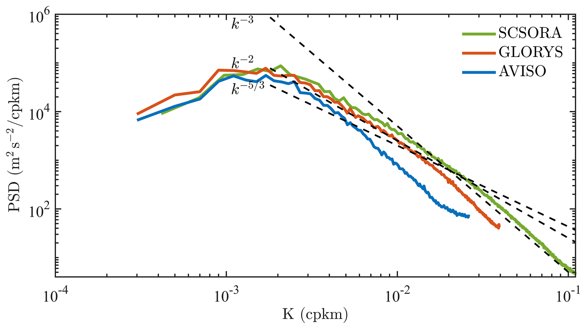
Figure 13One-dimensional horizontal wavenumber power spectral density (PSD) of sea surface velocity from SCSORA (green), GLORYS (orange), and AVISO (blue). The horizontal axis K denotes spatial wavenumber (cpkm) and the vertical axis denotes spectral energy density (m2 s−2 cpkm−1). Black dashed lines indicate theoretical spectral slopes of k−3 (Interior Quasigeostrophy), k−2 (Surface Quasigeostrophy with Ageostrophic Advection), and (Surface Quasigeostrophy), serving as references for evaluating the energy distribution characteristics and turbulent dynamics consistency of each product across different spatial scales.
4.2 Spatiotemporal Characteristics of Heatwaves
MHWs are widely recognized as important drivers of marine ecosystem stress and regional climate variability (Frölicher et al., 2018; Oliver et al., 2018). The combination of high-resolution temperature data with dynamical process information is essential for understanding the spatial distribution and intensity evolution of MHWs. Statistical results for the period 2001–2024 indicate that the spatial distributions of MHW characteristics derived from SCSORA and OSTIA are broadly consistent (Fig. 14), with both datasets exhibiting pronounced spatial heterogeneity: MHW frequency in the NSCS is substantially higher than in the southern SCS, and maximum intensity likewise displays a north-high, south-low spatial pattern. The regions of strongest MHW intensity in both SCSORA and OSTIA are located at the Taiwan Strait. Compared with OSTIA, SCSORA resolves richer mesoscale spatial variability. The spatial distribution of mean MHW intensity is broadly consistent between the two products, with mean intensity generally below 1.5 °C in the southern SCS and increasing progressively northward along the coastline.
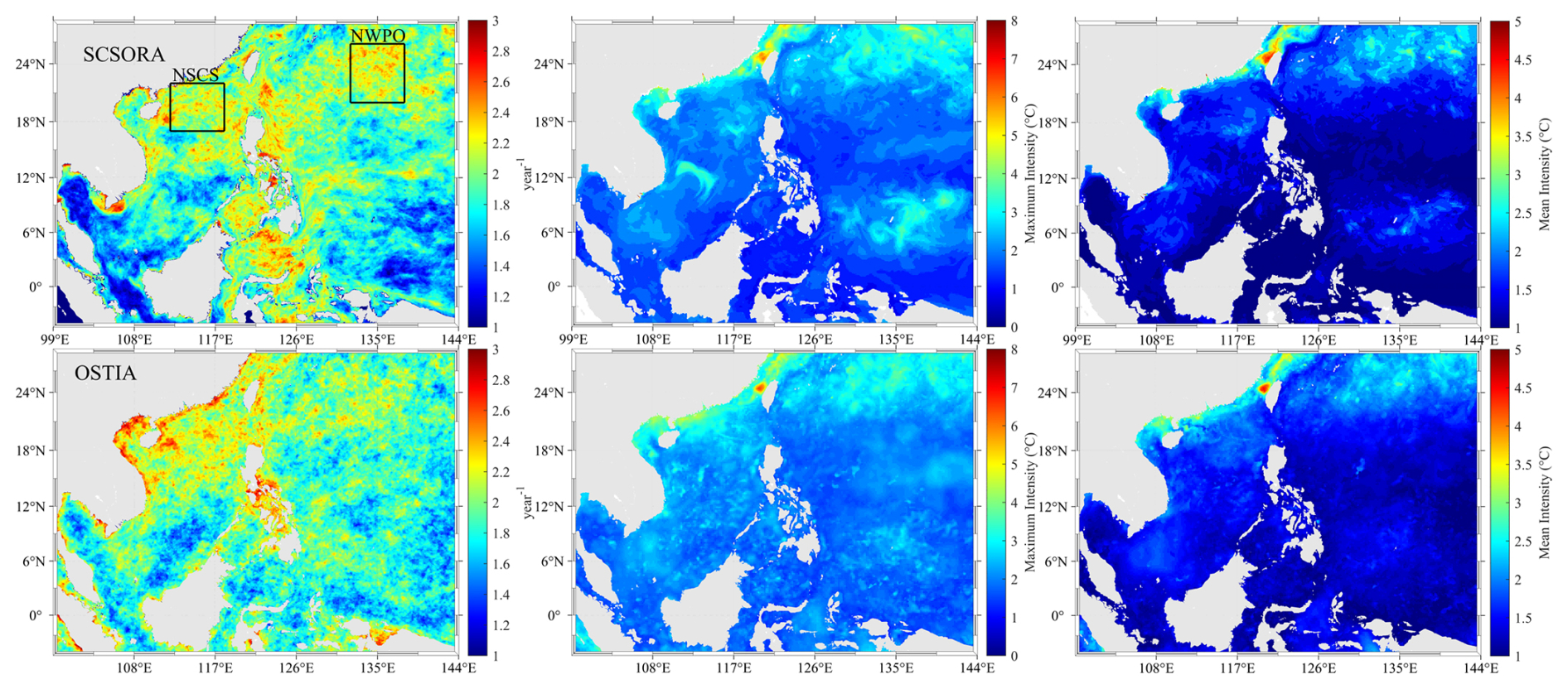
Figure 14Spatial distribution of climatological marine heatwave (MHW) characteristics from SCSORA (top row) and OSTIA (bottom row), including annual MHW frequency (left column, units: events yr−1), maximum intensity (middle column, units: °C), and mean intensity (right column, units: °C). Black boxes in the left column denote the NSCS and northwestern Pacific Ocean (NWPO) subregions selected for further analysis.
Two characteristic subregions, the NSCS and the NWPO, are selected to analyze the interannual variability of MHWs (Fig. 15). In both subregions, SCSORA, OSTIA, and OISST show overall consistency in the interannual variability of MHW frequency, duration, and cumulative intensity, all exhibiting an increasing trend that becomes particularly evident after 2010. In the NSCS, MHW events count during 2000–2010 are generally low and relatively stable, with no more than two events per year. From 2010 onwards, MHW events become progressively more frequent and longer-lasting, with SCSORA recording up to seven events in individual years, durations reaching 19 d, and cumulative intensities exceeding 25 °C days. In the NWPO, all three products reveal a pronounced intensification of MHW activity around 2015–2016, which closely coincides with the strong El Niño event of 2015–2016. ENSO modulates the occurrence of MHWs through atmospheric teleconnections that favour the seasonal persistence of large-scale high-pressure ridge systems, suppressing local vertical mixing and cooling, thereby providing favourable thermodynamic background conditions for the onset and maintenance of MHWs in this region (Holbrook et al., 2019; Sen Gupta et al., 2020; Gregory et al., 2024; Xie et al., 2025). Following a relatively quiescent period during 2017–2018, MHW activities reach another peak in 2020. In 2020, OISST shows the highest peaks in both MHW frequency and cumulative intensity, followed by SCSORA, with OSTIA exhibiting the lowest values among the three. This intensification is consistent with record-breaking MHW events reported in the northwestern Pacific Ocean in recent studies (Cheung and Frölicher, 2020; Noh et al., 2023), which are closely associated with anomalous strengthening of the western North Pacific subtropical high (WNPSH). This anomalous circulation pattern promotes sustained sea surface warming by enhancing shortwave radiation, reducing wind speed, and suppressing evaporative cooling, while La Niña-type background conditions and oceanic heat advection further amplify regional heat accumulation (Chen et al., 2023; Han et al., 2023; Yao et al., 2023). SCSORA records a cumulative intensity exceeding 25 °C days in 2024, the highest value throughout the record period, while OISST shows a comparably high value and OSTIA exhibits a relatively lower peak.
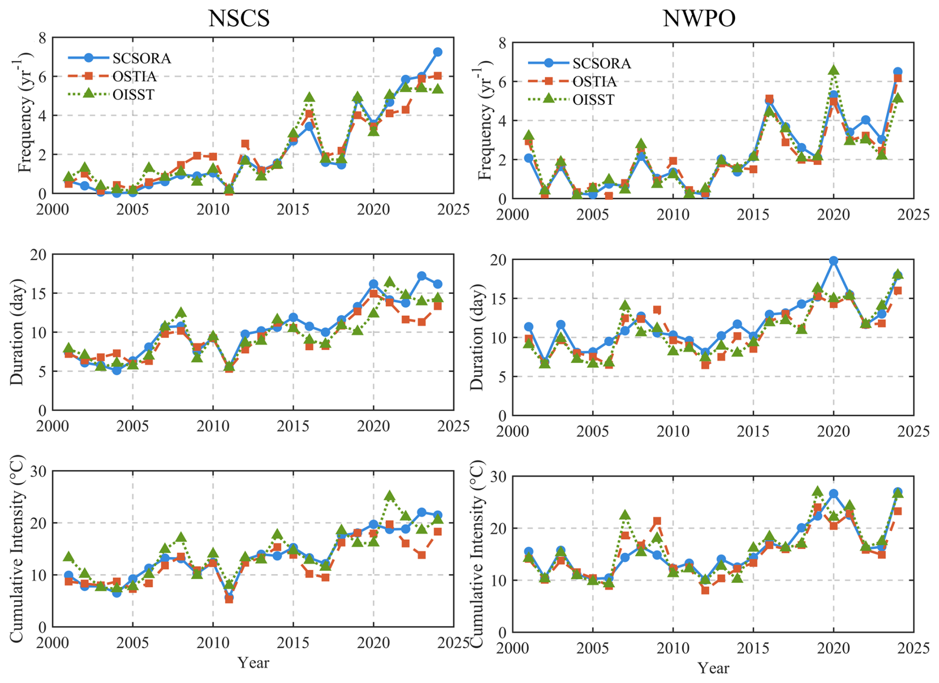
Figure 15Interannual variability of marine heatwave (MHW) characteristics in the NSCS (left column) and the NWPO (right column) during 2001–2024, including annual frequency (top row, units: yr−1), mean duration (middle row, units: days), and cumulative intensity (bottom row, units: °C).
Figure 16 presents the daily SST, climatology, and MHW thresholds based on SCSORA, OSTIA, and OISST for the NSCS and NWPO subregions in 2024, with MHW events exceeding the threshold marked by red shading. Overall, the three products exhibit a consistent seasonal cycle: SST reaches its minimum value during January–March and its peak value during June–September, while the threshold curve lies distinctly above the climatology, defining the identification criterion for MHWs (Hobday et al., 2016). In the NSCS, all three products identify significant summer MHW events, but differences exist at the event scale. The SCSORA SST time series is relatively smooth with weaker high-frequency fluctuations, resulting in longer event durations (up to 34 d) and slightly lower peak intensities (0.71 °C). OSTIA is more sensitive to high-frequency variability, capable of capturing shorter events (up to 23 d), with slightly higher peak intensities (0.75 °C). In the NWPO, the MHW signal is generally weaker, with lower duration and intensity; the strongest events recorded by the three products differ, with SCSORA at 0.64 °C, OSTIA at 0.46 °C, and OISST at 0.53 °C. OISST exhibits a variation trend broadly consistent with SCSORA, but with MHW intensity and MHW duration slightly lower than those of SCSORA.
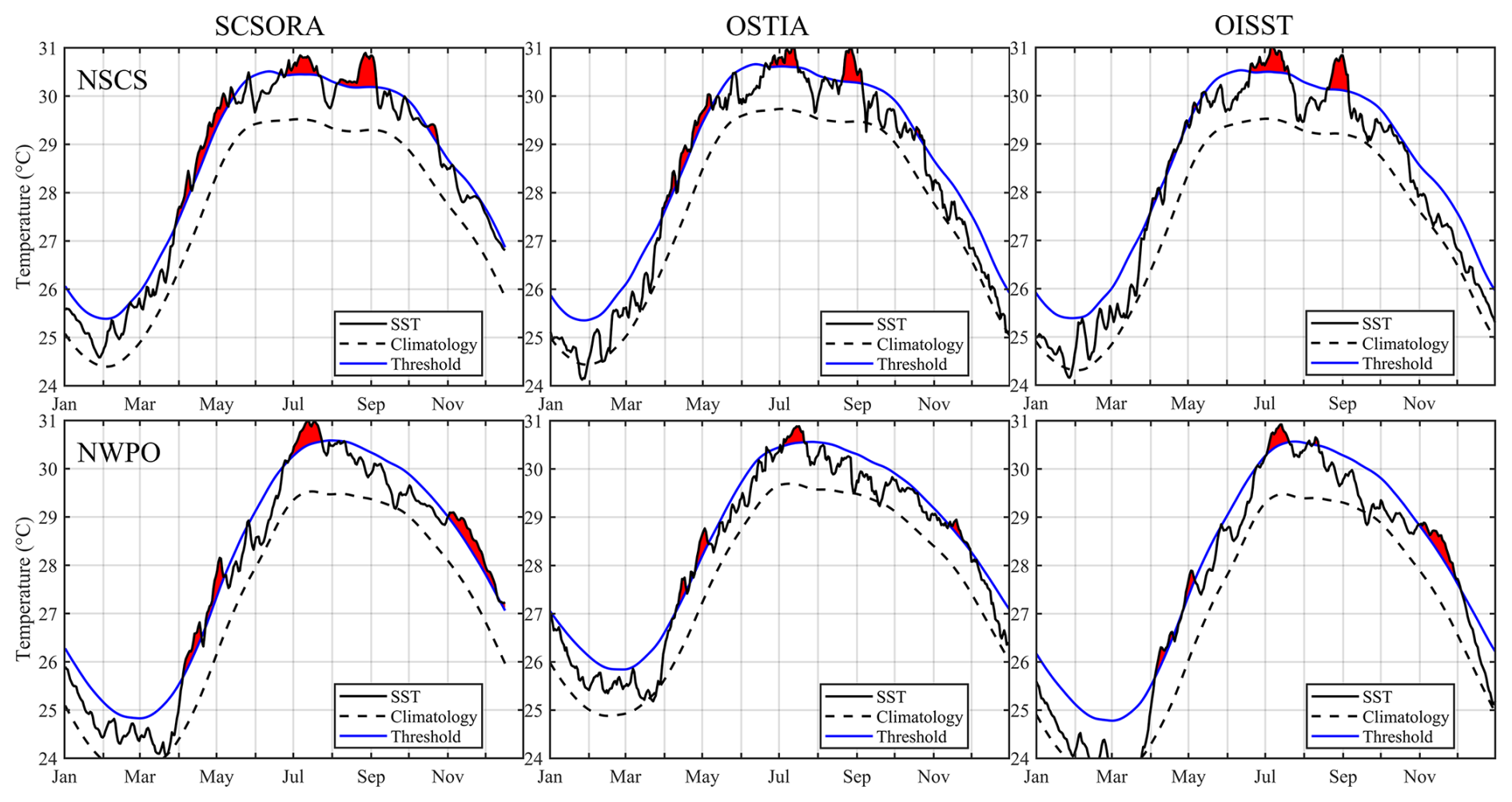
Figure 16Seasonal evolution of area-averaged SST from SCSORA (left column), OSTIA (middle column), and OISST (right column) in the NSCS (top row) and the NWPO (bottom row) for the year 2024. Black solid lines indicate daily mean SST in 2024, black dashed lines indicate climatological mean SST, and blue solid lines indicate the MHW threshold (90th percentile of climatology). Red shading denotes marine heatwave (MHW) events where daily SST exceeds the threshold.
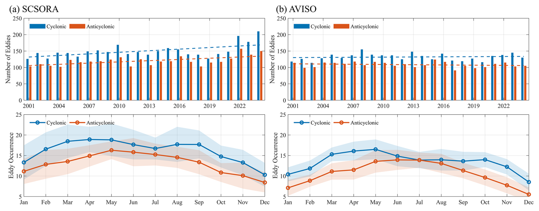
Figure 17Statistical characteristics of cyclonic (blue) and anticyclonic (orange) eddies in the SCS identified from SCSORA (left column) and AVISO (right column). Top row shows the interannual variation in eddy numbers during 2001–2024, with dashed lines indicating the corresponding linear trends. Bottom row shows the monthly climatological eddy occurrence, with solid lines representing multi-year monthly means and shading indicating the interannual variability range for each month.
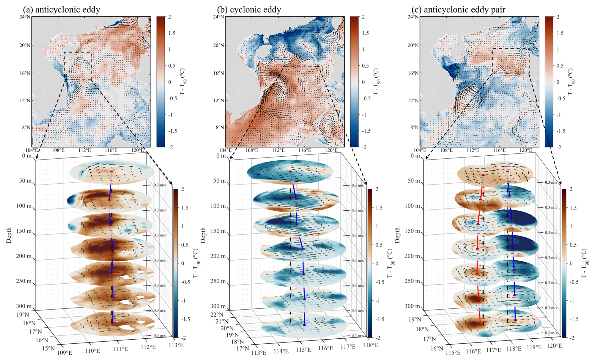
Figure 183D structure of MHWs in representative eddy-controlled regions. Left, middle, and right columns correspond to an anticyclonic eddy, a cyclonic eddy, and a compound double-anticyclonic eddy structure, respectively. Top row shows the SST anomaly (T−T90, units: °C) with black arrows indicating surface currents and black dashed boxes marking the eddy-influenced region. Bottom row shows the 3D vertical structure of MHW temperature anomalies (T−T90) within the corresponding eddy region (depth range: 0–300 m), with black arrows on each horizontal slice indicating the current field at that depth level, and vertical colored lines marking the eddy center positions and their lateral displacement with depth
4.3 Mesoscale Eddy Dynamics and Marine Heatwave Modulation
The statistical results indicate that in the eddy-active region of the SCS (102–122° E, 5–24° N), cyclonic eddies outnumber anticyclonic eddies (Fig. 17). SCSORA and AVISO are generally consistent in interannual variability, but SCSORA identifies a slightly higher number of eddies, especially during 2022–2024. Notably, both AVISO and SCSORA exhibit an increasing trend during 2020–2023, with a more pronounced increase in SCSORA, especially during 2022–2024. Eddy activity in the SCS is modulated by the monsoon, ENSO, and PDO through local wind stress curl (Wang et al., 2003; Cheng and Qi, 2010; He et al., 2016). The negative PDO and consecutive La Niña conditions in the 2020s may favor cyclonic eddy generation; meanwhile, the Kuroshio intrusion through the Luzon Strait can enhance frontal and shear instability in the NSCS, also favoring the generation of new eddies (Wu and Chiang, 2007). In addition, differences in effective resolution among datasets may also affect the comparison of eddy counts. Such method- and resolution-dependent discrepancies are common in eddy detection and eddy data products (Dong et al., 2025). However, the specific mechanisms can only be clarified through dedicated sensitivity experiments and validation against higher-resolution observations. In terms of seasonal variability (bottom row of Fig. 17), cyclonic eddies exhibit a bimodal distribution, with two peaks occurring in March–May and August–October, respectively. In contrast, the seasonal variability of anticyclonic eddies is weaker, manifesting only as a single broad peak in May–August.
While most MHW studies based on the 90th percentile threshold have focused on the 2D distribution of SST anomalies (He et al., 2024; Oliver et al., 2021; Sun et al., 2026; Wyatt et al., 2023; Yao and Wang, 2024), the limited availability of 3D temperature data has hindered analysis of their subsurface structure. Mesoscale eddies themselves possess complex three-dimensional structures, including vertical tilt and subsurface coherence (Zhang et al., 2024), which may further modulate the subsurface structure of MHWs. Using SCSORA, we present illustrative examples of the three-dimensional (3D) structure of MHWs under three representative eddy configurations: an anticyclonic eddy, a cyclonic eddy, and a double-anticyclonic eddy pair (Fig. 18). The analysis covers the upper 300 m, with temperature anomalies defined as T−T90 and surface and subsurface currents shown as vectors.
In the anticyclonic eddy case (Fig. 18a), positive MHW temperature anomalies appear at all depth levels, with values exceeding 1.5 °C near the surface and remaining positive below 200 m, indicating that the MHW signal extends well into the subsurface. In the cyclonic eddy case (Fig. 18b), positive anomalies are weak at the eddy center but form arc- or ring-shaped patterns at the eddy periphery, with anomalies reaching approximately 1 °C. This produces a center-weak, edge-strong structure that is not evident from SST alone. In the double-anticyclonic eddy case (Fig. 18c), both eddies show positive surface anomalies, but their subsurface structures differ: one exhibits a subsurface-enhanced MHW with positive anomalies extending below 200 m, while the other displays a subsurface-reversed (cooling) anomaly, with negative values emerging below the surface layer. The colored vertical lines in Fig. 18 further indicate that the eddy centers are not perfectly vertical but shift laterally with depth, suggesting that the 3D structure of MHWs is closely tied to the vertical coherence of the eddy field.
These examples demonstrate that SCSORA can resolve the 3D structure of MHWs under different eddy configurations and can serve as a useful data basis for investigating eddy–MHW interactions. A comprehensive dynamical interpretation, however, is beyond the scope of this data-oriented paper and requires further analysis with independent observations.
The SCSORA dataset is publicly released in NetCDF format at https://doi.org/10.12378/geodb.2026.2.005.V1 (Zhu and Zhang, 2026) and will be updated on a rolling basis.
The present study proposes a long-term, high-resolution () oceanic reanalysis dataset for the SCS, named as SCSORA, covering the period 2001–2024, based on the SCSOFSv2, providing daily mean fields of 3D temperature, salinity, density, current velocity, and 2D SSH. The system employs the EnOI method in conjunction with the FGAT approach to handle asynchronous observations, assimilating satellite-derived OISST, AVISO Level 3 along-track satellites SLA, and in-situ temperature–salinity Argo profiles. Validation against publicly available observational datasets demonstrates that SST RMSE remains stable within the range of 0.25–0.45 °C (mean 0.357 °C relative to OSTIA) and SLA RMSE within 4.5–9.7 cm (mean 5.9 cm), indicating that SCSORA reliably reproduces both short-term oceanic variability and long-term trends. Comparison with 174,696 Global Drifter Program (GDP) samples during 2001–2024 further shows that SCSORA reproduces the main SCS surface circulation and seasonal variability, with mean RMSDs of 17.21, 16.73, and 15.50 cm s−1 for the U component, V component, and current speed, respectively. Vertical temperature and salinity biases are generally maintained within ±1.5 °C and ±0.2 PSU, respectively, and converge substantially below 200 m depth. Frequency–wavenumber spectral analysis shows that SCSORA resolves spectral energy extending to higher wavenumbers. SCSORA is capable of capturing multiscale ocean dynamical processes, including mesoscale and partially submesoscale eddy activity, eddy-driven vertical transport, and mixed processes, and successfully reproduces the spatial distribution, occurrence frequency, and intensity characteristics of MHWs. It can also provide data support for studies related to the 3D eddy-embedded heatwave structure formed under eddy modulation. The high resolution and 3D nature of SCSORA provide more reliable data support for analyses of seasonal and interannual variability in the SCS, validation of regional ocean models, and long-term climate change monitoring.
Conceptualization: XMZ; Data curation: XMZ, XRZ; Formal analysis: XMZ, XRZ; Funding acquisition: XMZ; Investigation: XRZ, HLW; Methodology: XMZ, ZZ, GL, JL; Project administration: XMZ, HW; Software: XMZ, ZZ, GL; Supervision: XMZ, HW; Validation: XRZ, HLW; Visualization: XRZ; Writing – original draft: XRZ; Writing – review & editing: XMZ, XRZ. All authors have read and agreed to the published version of the manuscript.
The contact author has declared that none of the authors has any competing interests.
Publisher's note: Copernicus Publications remains neutral with regard to jurisdictional claims made in the text, published maps, institutional affiliations, or any other geographical representation in this paper. The authors bear the ultimate responsibility for providing appropriate place names. Views expressed in the text are those of the authors and do not necessarily reflect the views of the publisher.
We thank all colleagues and project members who contributed to the development of the SCSOFSv2 system and the production of the SCSORA dataset. We are grateful to the scientists, engineers, and students involved in the collection of in-situ observations, data processing, and system maintenance. We also acknowledge the providers of satellite, reanalysis products, and in-situ datasets used in this study. Their long-term efforts in data collection and open data sharing made this work possible.
This research has been supported by the Southern Marine Science and Engineering Guangdong Laboratory (Zhuhai) under grant numbers SML2024SP023 and SML2023SP202, the National Natural Science Foundation of China (Grant Nos. 42176029), and the Ocean Negative Carbon Emission (ONCE) Program.
This paper was edited by François G. Schmitt and reviewed by two anonymous referees.
An, M., Liu, J., Liu, J., Sun, W., Yang, J., Tan, W., Liu, Y., Sian, K. T. C. L. K., Ji, J., and Dong, C.: Comparative analysis of four types of mesoscale eddies in the north pacific subtropical countercurrent region – Part I spatial characteristics, Front. Mar. Sci., 9, 1004300, https://doi.org/10.3389/fmars.2022.1004300, 2022.
Archer, M. R., Li, Z., and Fu, L. L.: Increasing the space–time resolution of mapped sea surface height from altimetry, J. Geophys. Res.-Oceans, 125, e2019JC015878, https://doi.org/10.1029/2019JC015878, 2020.
Argo Science Team: On the design and implementation of Argo: An initial plan for a global array of profiling floats, GODAE International Project Office, https://argo.ucsd.edu/wp-content/uploads/sites/361/2020/05/argo-design.pdf (last access: 12 December 2025), 1998.
Bian, C., Jing, Z., Wang, H., Wu, L., Chen, Z., Gan, B., and Yang, H.: Oceanic mesoscale eddies as crucial drivers of global marine heatwaves, Nat. Commun., 14, 2970, https://doi.org/10.1038/s41467-023-38811-z, 2023.
Cai, Z., Gan, J., Liu, Z., Hui, C. R., and Li, J.: Progress on the formation dynamics of the layered circulation in the South China Sea, Prog. Oceanogr., 181, 102246, https://doi.org/10.1016/j.pocean.2019.102246, 2020.
Callies, J., Ferrari, R., Klymak, J., and Gula, J.: Seasonality in submesoscale turbulence, Nat. Commun., 6, 6862, https://doi.org/10.1038/ncomms7862, 2015.
Capet, X., McWilliams, J. C., Molemaker, M. J., and Shchepetkin, A. F.: Mesoscale to submesoscale transition in the California current system. Part I: flow structure, eddy flux, and observational tests, J. Phys. Oceanogr., 38, 29–43, https://doi.org/10.1175/2007JPO3671.1, 2008.
Carnes, M. R.: Description and evaluation of GDEM-V 3.0, Naval Research Laboratory, Stennis Space Center, MS, NRL/MR/7330-09-9165, https://www7320.nrlssc.navy.mil/pubs/2009/carnes-2009.pdf (last access: 4 February 2026), 2009.
Castillo-Trujillo, A. C., Kwon, Y. O., Fratantoni, P., Chen, K., Seo, H., Alexander, M. A., and Saba, V. S.: An evaluation of eight global ocean reanalyses for the Northeast US continental shelf, Prog. Oceanogr., 219, 103126, https://doi.org/10.1016/j.pocean.2023.103126, 2023.
Chapman, D. C.: Numerical treatment of cross-shelf open boundaries in a barotropic coastal ocean model, J. Phys. Oceanogr., 15, 1060–1075, 1985.
Chen, G., Hou, Y., and Chu, X.: Mesoscale eddies in the South China Sea: Mean properties, spatiotemporal variability, and impact on thermohaline structure, J. Geophys. Res.-Oceans, 116, C06018, https://doi.org/10.1029/2010JC006716, 2011.
Chen, R., Yang, Y., Geng, Q., Stewart, A., Flierl, G., and Wang, J.: Diagnostic framework linking eddy flux ellipse with eddy-mean energy exchange, Ocean-Land-Atmos. Res., 3, 0072, https://doi.org/10.34133/olar.0072, 2024.
Chen, Y., Xiao, C., Zhang, Y., and Lai, Z.: The mixed layer salinity budget in the Northern South China Sea: a modeling study, J. Mar. Sci. Eng., 11, 1693, https://doi.org/10.3390/jmse11091693, 2023.
Cheng, L., Abraham, J., Trenberth, K. E., Boyer, T., Mann, M. E., Zhu, J., and Lu, Y.: New record ocean temperatures and related climate indicators in 2023, Adv. Atmos. Sci., 41, 1068–1082, https://doi.org/10.1007/s00376-024-3378-5, 2024a.
Cheng, L., Pan, Y., Tan, Z., Zheng, H., Zhu, Y., Wei, W., Du, J., Yuan, H., Li, G., Ye, H., Gouretski, V., Li, Y., Trenberth, K. E., Abraham, J., Jin, Y., Reseghetti, F., Lin, X., Zhang, B., Chen, G., Mann, M. E., and Zhu, J.: IAPv4 ocean temperature and ocean heat content gridded dataset, Earth Syst. Sci. Data, 16, 3517–3546, https://doi.org/10.5194/essd-16-3517-2024, 2024b.
Cheng, X. and Qi, Y.: Variations of eddy kinetic energy in the South China Sea, J. Oceanogr., 66, 85–94, 2010.
Cheung, W. W. L. and Frölicher, T. L.: Marine heatwaves exacerbate climate change impacts for fisheries in the northeast Pacific, Sci. Rep., 10, 6678, https://doi.org/10.1038/s41598-020-63650-z, 2020.
Copernicus Marine Service: Global Ocean Gridded L4 Sea Surface Heights and Derived Variables Reprocessed 1993 Ongoing, Mercator Ocean International [data set], https://doi.org/10.48670/moi-00148, 2024a.
Copernicus Marine Service: Global Ocean OSTIA Sea Surface Temperature and Sea Ice Reprocessed, Mercator Ocean International [data set], https://doi.org/10.48670/moi-00168, 2024b.
Cummings, J. A. and Smedstad, O. M.: Variational data assimilation for the global ocean, in: Data Assimilation for Atmospheric, Oceanic and Hydrologic Applications, Vol. II, Springer, Berlin, Heidelberg, 303–343, https://doi.org/10.1007/978-3-642-35088-7_13, 2013.
Dong, C., You, Z., Dong, J., Ji, J., Sun, W., Xu, G., Lu, X., Xie, H., Teng, F., Liu, Y., Xu, A., Wang, Q., Xia, Q., Lin, X., Fu, M., Wang, J., Cao, Y., and Han, G.: Oceanic mesoscale eddies, Ocean-Land-Atmos. Res., 4, 0081, https://doi.org/10.34133/olar.0081, 2025.
Donlon, C. J., Martin, M., Stark, J., Roberts-Jones, J., Fiedler, E., and Wimmer, W.: The operational sea surface temperature and sea ice analysis (OSTIA) system, Remote Sens. Environ., 116, 140–158, https://doi.org/10.1016/j.rse.2010.10.017, 2012.
Elipot, S., Lumpkin, R., Perez, R. C., Lilly, J. M., Early, J. J., and Sykulski, A. M.: A global surface drifter data set at hourly resolution, J. Geophys. Res.-Oceans, 121, 2937–2966, https://doi.org/10.1002/2016JC011716, 2016.
Evans, D. G., Frajka-Williams, E., and Garabato, A. N.: Dissipation of mesoscale eddies at a western boundary via a direct energy cascade, Sci. Rep., 12, 887, https://doi.org/10.1038/s41598-022-05002-7, 2022.
Evensen, G.: The ensemble Kalman filter: theoretical formulation and practical implementation, Ocean Dynam., 53, 343–367, https://doi.org/10.1007/s10236-003-0036-9, 2003.
Ferrari, R. and Wunsch, C.: Ocean circulation kinetic energy: Reservoirs, sources, and sinks, Annu. Rev. Fluid Mech., 41, 253–282, https://doi.org/10.1146/annurev.fluid.40.111406.102139, 2009.
Flather, R. A.: A tidal model of the northwest European continental shelf, Mem. Soc. R. Sci. Liege, 10, 141–164, http://pascal-francis.inist.fr/vibad/index.php?action=getRecordDetail&idt=PASCAL7730150079 (last access: 12 February 2026), 1976.
Frölicher, T. L., Fischer, E. M., and Gruber, N.: Marine heatwaves under global warming, Nature, 560, 360–364, https://doi.org/10.1038/s41586-018-0383-9, 2018.
Gregory, C. H., Artana, C., Lama, S., León-FonFay, D., Sala, J., Xiao, F., and Holbrook, N. J.: Global marine heatwaves under different flavors of ENSO, Geophys. Res. Lett., 51, e2024GL110399, https://doi.org/10.1029/2024GL110399, 2024.
Guo, M., Xiu, P., Li, S., Chai, F., Xue, H., Zhou, K., and Dai, M.: Seasonal variability and mechanisms regulating chlorophyll distribution in mesoscale eddies in the South China Sea, J. Geophys. Res.-Oceans, 122, 5329–5347, https://doi.org/10.1002/2016JC012670, 2017.
Guo, P., Zhao, M., and Lian, Z.: El Niño enhances coral larval dispersal potential of Dongsha Island – a biodiversity hotspot in the South China Sea, Front. Mar. Sci., 13, 1748933, https://doi.org/10.3389/fmars.2026.1748933, 2026.
Han, T., Xu, K., Wang, L., Liu, B., Tam, C. Y., Liu, K., and Wang, W.: Extremely long-lived marine heatwave in South China Sea during summer 2020: Combined effects of the seasonal and intraseasonal variations, Global Planet. Change, 230, 104261, https://doi.org/10.1016/j.gloplacha.2023.104261, 2023.
He, Q., Zhan, W., Feng, M., Gong, Y., Cai, S., and Zhan, H.: Common occurrences of subsurface heatwaves and cold spells in ocean eddies, Nature, 634, 1111–1117, https://doi.org/10.1038/s41586-024-08051-2, 2024.
He, R., Wu, T., Mao, S., Zong, H., Zambon, J., Warrillow, J., and Hernandez, D.: Advanced Ocean Reanalysis of the Northwestern Atlantic: 1993–2022, arxiv [preprint], https://doi.org/10.48550/arXiv.2503.06907, 2025.
He, Y., Xie, J., and Cai, S.: Interannual variability of winter eddy patterns in the eastern South China Sea, Geophys. Res. Lett., 43, 5185–5193, https://doi.org/10.1002/2016GL068842, 2016.
Hersbach, H., Bell, B., Berrisford, P., Hirahara, S., Horányi, A., Muñoz-Sabater, J., Nicolas, J., Peubey, C., Radu, R., Schepers, D., Simmons, A., Soci, C., Abdalla, S., Abellan, X., Balsamo, G., Bechtold, P., Biavati, G., Bidlot, J., Bonavita, M., De Chiara, G., Dahlgren, P., Dee, D., Diamantakis, M., Dragani, R., Flemming, J., Forbes, R., Fuentes, M., Geer, A., Haimberger, L., Healy, S., Hogan, R. J., Hólm, E., Janisková, M., Keeley, S., Laloyaux, P., Lopez, P., Lupu, C., Radnoti, G., de Rosnay, P., Rozum, I., Vamborg, F., Villaume, S., and Thépaut, J.-N.: The ERA5 global reanalysis, Q. J. Roy. Meteor. Soc., 146, 1999–2049, https://doi.org/10.1002/qj.3803, 2020.
Hobday, A. J., Alexander, L. V., Perkins, S. E., Smale, D. A., Straub, S. C., Oliver, E. C., and Wernberg, T.: A hierarchical approach to defining marine heatwaves, Prog. Oceanogr., 141, 227–238, https://doi.org/10.1016/j.pocean.2015.12.014, 2016.
Holbrook, N. J., Scannell, H. A., Sen Gupta, A., Benthuysen, J. A., Feng, M., Oliver, E. C., and Wernberg, T.: A global assessment of marine heatwaves and their drivers, Nat. Commun., 10, 2624, https://doi.org/10.1038/s41467-019-10206-z, 2019.
Hughes, T. P., Kerry, J. T., Baird, A. H., Connolly, S. R., Dietzel, A., Eakin, C. M., Heron, S. F., Hoey, A. S., Hoogenboom, M. O., Liu, G., McWilliam, M. J., Pears, R. J., Pratchett, M. S., Skirving, W. J., Stella, J. S., and Torda, G.: Global warming transforms coral reef assemblages, Nature, 556, 492–496, https://doi.org/10.1038/s41586-018-0041-2, 2018.
Jean-Michel, L., Eric, G., Romain, B. B., Gilles, G., Angélique, M., Marie, D., and Pierre-Yves, L. T.: The Copernicus global 1/12 oceanic and sea ice GLORYS12 reanalysis, Front. Earth Sci., 9, 698876, https://doi.org/10.3389/feart.2021.698876, 2021.
Jin, Y., Jin, M., Wang, D., and Dong, C.: Statistical analysis of multi-year South China Sea eddies and exploration of eddy classification, Remote Sens., 16, 1818, https://doi.org/10.3390/rs16101818, 2024.
Juhl, M. C., Passaro, M., and Dettmering, D.: Regional daily sea level maps from multi-mission altimetry using space–time window Kriging, Adv. Space Res., 75, 7769–7786, https://doi.org/10.1016/j.asr.2025.04.014, 2025.
Kerry, C. G., Roughan, M., Keating, S., Gwyther, D., Brassington, G., Siripatana, A., and Souza, J. M. A. C.: Comparison of 4-dimensional variational and ensemble optimal interpolation data assimilation systems using a Regional Ocean Modeling System (v3.4) configuration of the eddy-dominated East Australian Current system, Geosci. Model Dev., 17, 2359–2386, https://doi.org/10.5194/gmd-17-2359-2024, 2024.
Kim, W., Yeh, S. W., Kim, J. H., Kug, J. S., and Kwon, M.: The unique 2009–2010 El Niño event: A fast phase transition of warm pool El Niño to La Niña, Geophys. Res. Lett., 38, L15809, https://doi.org/10.1029/2011GL048521, 2011.
Kuo, Y.-C., Chan, J.-W., Wang, Y.-C., Shen, Y.-L., Chang, Y., and Lee, M.-A.: Long-term observation on sea surface temperature variability in the Taiwan Strait during the northeast monsoon season, Int. J. Remote Sens., 39, 4330–4342, https://doi.org/10.1080/01431161.2017.1387311, 2018.
Lguensat, R., Viet, P. H., Sun, M., Chen, G., Fenglin, T., Chapron, B., and Fablet, R.: Data-driven interpolation of sea level anomalies using analog data assimilation, Remote Sens., 11, 858, https://doi.org/10.3390/rs11070858, 2019.
Li, Z., Jiang, X., and Wang, G.: Numerical models, observing systems, and data assimilation for prediction of ocean mesoscale eddies, Ocean-Land-Atmos. Res., 3, 0059, https://doi.org/10.34133/olar.0059, 2024.
Li, Y., Ren, G., Wang, Q., Mu, L., and Niu, Q.: Marine heatwaves in the South China Sea: tempo-spatial pattern and its association with large-scale circulation, Remote Sens., 14, 5829, https://doi.org/10.3390/rs14225829, 2022.
Lin, X., Dong, C., Chen, D., Liu, Y., Yang, J., Zou, B., and Guan, Y.: Three-dimensional properties of mesoscale eddies in the South China Sea based on eddy-resolving model output, Deep-Sea Res. Pt. I, 99, 46–64, https://doi.org/10.1016/j.dsr.2015.01.007, 2015.
Lumpkin, R. and Pazos, M.: Measuring surface currents with Surface Velocity Program drifters: the instrument, its data, and some recent results, in: Lagrangian Analysis and Prediction of Coastal and Ocean Dynamics, edited by: Griffa, A., Kirwan, A. D., Mariano, A. J., Özgökmen, T., and Ross, T., Cambridge University Press, 39–67, https://doi.org/10.1017/CBO9780511535901.003, 2007.
Lumpkin, R., Özgökmen, T., and Centurioni, L.: Advances in the application of surface drifters, Annu. Rev. Mar. Sci., 9, 59–81, https://doi.org/10.1146/annurev-marine-010816-060641, 2017
Madin, E. M.: Halt reef destruction in South China Sea, Nature, 524, 291–291, https://doi.org/10.1038/524291a, 2015.
Marchesiello, P., McWilliams, J. C., and Shchepetkin, A.: Open boundary conditions for long-term integration of regional oceanic models, Ocean Model., 3, 1–20, https://doi.org/10.1016/S1463-5003(00)00013-5, 2001.
Mellor, G. L. and Yamada, T.: Development of a turbulence closure model for geophysical fluid problems, Rev. Geophys., 20, 851–875, https://doi.org/10.1029/RG020i004p00851, 1982.
Nan, F., Xue, H., and Yu, F.: Kuroshio intrusion into the South China Sea: A review, Prog. Oceanogr., 137, 314–333, https://doi.org/10.1016/j.pocean.2014.05.012, 2015.
Nencioli, F., Dong, C., Dickey, T., Washburn, L., and McWilliams, J. C.: A vector geometry–based eddy detection algorithm and its application to a high-resolution numerical model product and high-frequency radar surface velocities in the Southern California Bight, J. Atmos. Ocean. Technol., 27, 564–579, https://doi.org/10.1175/2009JTECHO725.1, 2010.
Niiler, P. P.: The world ocean surface circulation, in: Ocean Circulation and Climate: Observing and Modelling the Global Ocean, edited by: Siedler, G., Church, J., and Gould, J., International Geophysics Series, Academic Press, 77, 193–204, https://doi.org/10.1016/S0074-6142(01)80119-4, 2001
Noh, E., Kim, J., Jun, S. Y., Pak, G., Kim, J.-H., and Kim, H.-G.: Atmospheric pathway of marine heatwaves over the Northwestern Pacific, Sci. Rep., 13, 22821, https://doi.org/10.1038/s41598-023-49833-4, 2023.
Oke, P. R., Brassington, G. B., Griffin, D. A., and Schiller, A.: The Bluelink ocean data assimilation system (BODAS), Ocean Model., 21, 46–70, https://doi.org/10.1016/j.ocemod.2007.11.002, 2008.
Oliver, E. C. J., Benthuysen, J. A., Darmaraki, S., Donat, M. G., Hobday, A. J., Holbrook, N. J., Schlegel, R. W., and Sen Gupta, A.: Marine heatwaves, Annu. Rev. Mar. Sci., 13, 313–342, https://doi.org/10.1146/annurev-marine-032720-095144, 2021.
Oliver, E. C. J., Donat, M. G., Burrows, M. T., Moore, P. J., Smale, D. A., Alexander, L. V., Benthuysen, J. A., Feng, M., Sen Gupta, A., Hobday, A. J., Holbrook, N. J., Perkins-Kirkpatrick, S. E., Scannell, H. A., Straub, S. C., and Wernberg, T.: Longer and more frequent marine heatwaves over the past century, Nat. Commun., 9, 1324, https://doi.org/10.1038/s41467-018-03732-9, 2018.
Pan, J. and Sun, Y.: Estimation of horizontal eddy heat flux in upper mixed-layer in the South China Sea by using satellite data, Sci. Rep., 8, 15527, https://doi.org/10.1038/s41598-018-33803-2, 2018.
Passaro, M. and Juhl, M. C.: On the potential of mapping sea level anomalies from satellite altimetry with Random Forest Regression, Ocean Dynam., 73, 107–116, https://doi.org/10.1007/s10236-023-01540-4, 2023.
Paul, N. and Mahadevan, A.: Near-inertial waves enhance vertical transport at ocean fronts, arXiv [preprint], https://doi.org/10.48550/arXiv.2511.23460, 2025.
Qiu, C., Du, Z., Tang, H., Yi, Z., Qiao, J., Wang, D., Zhai, X., and Wang, W.: A high-resolution temperature–salinity dataset observed by autonomous underwater vehicles for the evolution of mesoscale eddies and associated submesoscale processes in the South China Sea, Earth Syst. Sci. Data, 17, 3189–3202, https://doi.org/10.5194/essd-17-3189-2025, 2025a.
Qiu, C., Du, Z., Tang, H., Yi, Z., Qiao, J., Wang, D., Zhai, X., and Wang, W.: A High-Resolution Temperature-Salinity Dataset Observed by Autonomous Underwater Vehicles for the Evolution of Mesoscale Eddies and Associated Submesoscale Processes in South China Sea, Science Data Bank [data set], https://doi.org/10.57760/sciencedb.11996, 2025b.
Reynolds, R. W., Smith, T. M., Liu, C., Chelton, D. B., Casey, K. S., and Schlax, M. G.: Daily high-resolution-blended analyses for sea surface temperature, J. Climate, 20, 5473–5496, https://doi.org/10.1175/2007JCLI1824.1, 2007.
Rio, M. H., Santoleri, R., Bourdalle-Badie, R., Griffa, A., Piterbarg, L., and Taburet, G.: Improving the altimeter-derived surface currents using high-resolution sea surface temperature data: a feasibility study based on model outputs, J. Atmos. Ocean. Tech., 33, 2769–2784, https://doi.org/10.1175/JTECH-D-16-0017.1, 2016.
Roemmich, D., Johnson, G. C., Riser, S., Davis, R., Gilson, J., Owens, W. B., and Ignaszewski, M.: The Argo Program: Observing the global ocean with profiling floats, Oceanography, 22, 34–43, https://doi.org/10.5670/oceanog.2009.36, 2009.
Sallée, J. B., Pellichero, V., Akhoudas, C., Pauthenet, E., Vignes, L., Schmidtko, S., and Kuusela, M.: Summertime increases in upper-ocean stratification and mixed-layer depth, Nature, 591, 592–598, https://doi.org/10.1038/s41586-021-03303-x, 2021.
Schubert, R., Gula, J., Greatbatch, R. J., Baschek, B., and Biastoch, A.: The submesoscale kinetic energy cascade: Mesoscale absorption of submesoscale mixed layer eddies and frontal downscale fluxes, J. Phys. Oceanogr., 50, 2573–2589, https://doi.org/10.1175/JPO-D-19-0311.1, 2020.
Sen Gupta, A., Thomsen, M., Benthuysen, J. A., Hobday, A. J., Oliver, E., Alexander, L. V., Burrows, M. T., Donat, M. G., Feng, M., Holbrook, N. J., Perkins-Kirkpatrick, S., Moore, P. J., Rodrigues, R. R., Scannell, H. A., Taschetto, A. S., Ummenhofer, C. C., Wernberg, T., and Smale, D. A.: Drivers and impacts of the most extreme marine heatwave events, Sci. Rep., 10, 19359, https://doi.org/10.1038/s41598-020-75445-3, 2020.
Shchepetkin, A. F. and McWilliams, J. C.: The regional oceanic modeling system (ROMS): a split-explicit, free-surface, topography-following-coordinate oceanic model, Ocean Model., 9, 347–404, https://doi.org/10.1016/j.ocemod.2004.08.002, 2005.
Song, X., Sun, R., He, S., Zhang, H., Gu, Y., Li, P., and Song, J.: Impact of anticyclonic mesoscale eddies on the vertical structures of marine heatwaves in the South China Sea, Remote Sens., 17, 370, https://doi.org/10.3390/rs17030370, 2025.
Soufflet, Y., Marchesiello, P., Lemarié, F., Jouanno, J., Capet, X., Debreu, L., and Benshila, R.: On effective resolution in ocean models, Ocean Model., 98, 36–50, https://doi.org/10.1016/j.ocemod.2015.12.004, 2016.
Stammer, D.: Global characteristics of ocean variability estimated from regional TOPEX/POSEIDON altimeter measurements, J. Phys. Oceanogr., 27, 1743–1769, https://doi.org/10.1175/1520-0485(1997)027<1743:GCOOVE>2.0.CO;2, 1997.
Stammer, D.: On eddy characteristics, eddy transports, and mean flow properties, J. Phys. Oceanogr., 28, 727–739, https://doi.org/10.1175/1520-0485(1998)028<0727:OECETA>2.0.CO;2, 1998.
Sun, W., Wang, Y., Xie, M., Pan, Y., Li, C., Ji, J., and Dong, C.: Exploring the connection of marine heatwaves and mesoscale eddies in the South China Sea, J. Oceanol. Limnol., 1–15, https://doi.org/10.1007/s00343-025-4332-9, 2026.
Sun, W., Dong, C., Tan, W., and He, Y.: Statistical characteristics of cyclonic warm-core eddies and anticyclonic cold-core eddies in the North Pacific based on remote sensing data, Remote Sens., 11, 208, https://doi.org/10.3390/rs11020208, 2019.
Taburet, G., Sanchez-Roman, A., Ballarotta, M., Pujol, M.-I., Legeais, J.-F., Fournier, F., Faugere, Y., and Dibarboure, G.: DUACS DT2018: 25 years of reprocessed sea level altimetry products, Ocean Sci., 15, 1207–1224, https://doi.org/10.5194/os-15-1207-2019, 2019.
Tang, D., Sun, Z., and Sui, G.: Geological environment in the South China Sea, J. Oceanol. Limnol., 41, 403–408, https://doi.org/10.1007/s00343-023-3403-2, 2023.
Terhaar, J., Burger, F. A., Vogt, L., Frölicher, T. L., and Stocker, T. F.: Record sea surface temperature jump in 2023–2024 unlikely but not unexpected, Nature, 639, 942–946, https://doi.org/10.1038/s41586-025-08674-z, 2025.
Thompson, B. and Tkalich, P.: Mixed layer thermodynamics of the Southern South China Sea, Clim. Dynam., 43, 2061–2075, https://doi.org/10.1007/s00382-013-2030-3, 2014.
Thoppil, P. G.: Enhanced phytoplankton bloom triggered by atmospheric high-pressure systems over the Northern Arabian Sea, Sci. Rep., 13, 769, https://doi.org/10.1038/s41598-023-27785-z, 2023.
Villas Bôas, A. B., Lenain, L., Cornuelle, B. D., Gille, S. T., and Mazloff, M. R.: A broadband view of the sea surface height wavenumber spectrum, Geophys. Res. Lett., 49, e2021GL096699, https://doi.org/10.1029/2021GL096699, 2022.
Wang, B., Huang, F., Wu, Z., Yang, J., Fu, X., and Kikuchi, K.: Multi-scale climate variability of the South China Sea monsoon: A review, Dyn. Atmos. Oceans, 47, 15–37, https://doi.org/10.1016/j.dynatmoce.2008.09.004, 2009.
Wang, D.: Overview of the atmosphere and hydrological environment of the South China Sea, in: Ocean Circulation and Air-Sea Interaction in the South China Sea, Springer Nature Singapore, Singapore, 1–15, https://doi.org/10.1007/978-981-19-6262-2_1, 2022.
Wang, G., Su, J., and Chu, P. C.: Mesoscale eddies in the South China Sea observed with altimeter data, Geophys. Res. Lett., 30, 2121, https://doi.org/10.1029/2003GL018532, 2003.
Wang, H., Lu, Y., Zhai, L., Chen, X., and Liu, S.: Variations of surface marine heatwaves in the Northwest Pacific during 1993–2019, Front. Mar. Sci., 11, 1323702, https://doi.org/10.3389/fmars.2024.1323702, 2024.
Wu, C.-R. and Chiang, T.-L.: Mesoscale eddies in the northern South China Sea, Deep-Sea Res. Pt. II, 54, 1575–1588, https://doi.org/10.1016/j.dsr2.2007.05.008, 2007.
Wyatt, A. S. J., Leichter, J. J., Washburn, L., Kui, L., Edmunds, P. J., and Burgess, S. C.: Hidden heatwaves and severe coral bleaching linked to mesoscale eddies and thermocline dynamics, Nat. Commun., 14, 25, https://doi.org/10.1038/s41467-022-35550-5, 2023.
Xie, B., Sun, H., Liu, T., Jin, W., Lin, F., Meng, L., and Wang, Y.: Formation of record-breaking 2015/2016 winter marine heatwave in the northwest South China Sea, Front. Mar. Sci., 12, 1671389, https://doi.org/10.3389/fmars.2025.1671389, 2025.
Xie, J. and Zhu, J.: Ensemble optimal interpolation schemes for assimilating Argo profiles into a hybrid coordinate ocean model, Ocean Model., 33, 283–298, https://doi.org/10.1016/j.ocemod.2010.03.002, 2010.
Xie, S.-P., Xie, Q., Wang, D., and Liu, W. T.: Summer upwelling in the South China Sea and its role in regional climate variations, J. Geophys. Res.-Oceans, 108, 3261, https://doi.org/10.1029/2003JC001867, 2003.
Yao, Y. and Wang, C.: Variations in summer marine heatwaves in the South China Sea, J. Geophys. Res.-Oceans, 126, e2021JC017792, https://doi.org/10.1029/2021JC017792, 2021.
Yao, Y. and Wang, C.: Subsurface marine heatwaves in the South China Sea, J. Geophys. Res.-Oceans, 129, e2024JC021356, https://doi.org/10.1029/2024JC021356, 2024.
Yao, Y., Wang, C., and Wang, C.: Record-breaking 2020 summer marine heatwaves in the western North Pacific, Deep-Sea Res. Pt. II, 209, 105288, https://doi.org/10.1016/j.dsr2.2023.105288, 2023.
Yi, Z., Qiu, C., Wang, D., Cai, Z., Yu, J., and Shi, J.: Submesoscale kinetic energy induced by vertical buoyancy fluxes during the tropical cyclone Haitang, J. Geophys. Res.-Oceans, 129, e2023JC020494, https://doi.org/10.1029/2023JC020494, 2024.
Zeng, X., Peng, S., Li, Z., Zeng, Q., and Wang, D.: A reanalysis dataset of the South China Sea, Sci. Data, 1, 140052, https://doi.org/10.1038/sdata.2014.52, 2014.
Zhang, Z., Tian, J., Qiu, B., Zhao, W., Chang, P., Wu, D., and Wan, X.: Observed 3D structure, generation, and dissipation of oceanic mesoscale eddies in the South China Sea, Sci. Rep., 6, 24349, https://doi.org/10.1038/srep24349, 2016.
Zhang, Z., Wang, G., Wang, H., and Liu, H.: Three-dimensional structure of oceanic mesoscale eddies, Ocean-Land-Atmos. Res., 3, 0051, https://doi.org/10.34133/olar.0051, 2024.
Zhao, Z. and Marin, M.: A MATLAB toolbox to detect and analyze marine heatwaves, J. Open Source Softw., 4, 1124, https://doi.org/10.21105/joss.01124, 2019.
Zhu, X. and Zhang, X.: South China Sea Ocean Reanalysis (SCSORA) dataset, Southern Marine Science and Engineering Guangdong Laboratory (Zhuhai) [data set], 2001–2024, Version 1, https://doi.org/10.12378/geodb.2026.2.005.V1, 2026.
Zhu, X., Zu, Z., Ren, S., Zhang, M., Zhang, Y., Wang, H., and Li, A.: Improvements in the regional South China Sea Operational Oceanography Forecasting System (SCSOFSv2), Geosci. Model Dev., 15, 995–1015, https://doi.org/10.5194/gmd-15-995-2022, 2022.
Zhu, X., Guo, S., Chang, J., Zhang, X., Hu, Z., and Wang, H.: Full destruction of an anticyclonic eddy in the Northern South China Sea by Tropical Storm Mulan, Deep-Sea Res. Pt. I, 104500, https://doi.org/10.1016/j.dsr.2025.104500, 2025.