the Creative Commons Attribution 4.0 License.
the Creative Commons Attribution 4.0 License.
 | 17 Nov 2026
ALPAKAS: Alpine hydrographs and catchment attributes for karst springs

Pauline Thinius
Zhao Chen
Andreas Hartmann
Nico Goldscheider
Tanja Liesch
Gerhard Schubert
Stefan Broda
Approximately 40 % of the European Alps consist of karstifiable rock. Due to their distinct recharge, storage, and discharge properties, karst aquifers are key components of the hydrological cycle and water supply in the Alpine region. However, large-sample datasets enabling comparative and data-driven analyses of karst spring discharge are currently lacking. Here, we present ALPAKAS (ALPine hydrographs and catchment Attributes for KArst Springs), the first large-sample benchmark dataset specifically dedicated to karst springs. ALPAKAS comprises 242 daily and 182 hourly quality-controlled and consistently preprocessed discharge time series from karst spring stations distributed across the EU Strategy for the Alpine Region (EUSALP) area, with stations located in seven countries. The dataset is complemented by both existing catchment delineations and circular catchment approximations, catchment-aggregated meteorological time series at multiple spatial scales, and a comprehensive set of static catchment attributes describing topography, positioning, meteorology, land cover, soil properties, and hydrogeology. In addition, the dataset includes karst-specific indices directly derived from the karst spring hydrographs.
ALPAKAS is available via Zenodo at https://doi.org/10.5281/zenodo.19329693 (Joger et al., 2026) under an open-access licence and is accompanied by comprehensive documentation. By providing a harmonized, large-sample compilation of karst spring catchments across diverse Alpine settings, the dataset enables comparative analyses, model benchmarking, and robust assessments of hydrogeological processes and climate change impacts.
- Article
(4845 KB) - Full-text XML
- BibTeX
- EndNote


The European Alps (hereafter referred to as Alps), the largest mountain range in central Europe, contain the headwaters of the major river systems Rhine, Danube, Rhône and Po and are therefore referred to as “Europe's water tower” (Viviroli et al., 2007). The Alps are among the regions in Europe most strongly affected by climate change and are warming almost twice as much as the global mean (Kotlarski et al., 2023). Increasing temperatures reduce snow and ice storage and, together with changing precipitation regimes, lead to seasonal flow redistribution and increased hydrological variability (Beniston et al., 2018). Particularly in snow- and glacier-dominated regimes, a shift toward more precipitation falling as rain, combined with earlier and more intense melting processes in winter, is expected to result in higher winter discharges (Wagner et al., 2017; Moraga et al., 2021; Vremec et al., 2025). In addition, climate change is projected to induce shifts in land use and vegetation patterns that are closely linked to the water cycle (Rumpf et al., 2022; Rubel et al., 2017). Despite being among the most extensively studied mountain regions worldwide, implications for the water balance remain complex in the Alps, as pronounced topographic heterogeneity leads to strong spatiotemporal meteorological variability that is often inadequately captured by available monitoring networks (Bongiovanni et al., 2025).
Beyond surface water, groundwater resources play a crucial role in sustaining streamflow in high mountain regions (Somers and McKenzie, 2020). With ongoing glacier retreat, permafrost thaw and declining snowpack, mountain groundwater is expected to become increasingly important relative to other water sources (van Tiel et al., 2024). Around 41 % of global karst areas are located in mountain regions (Goldscheider et al., 2020). In the Alps, karstifiable rocks cover approximately 40 % of the surface area, highlighting the widespread relevance of karst systems for regional groundwater (Chen et al., 2017; Goldscheider et al., 2025). Karst aquifers are characterized by strong structural and hydraulic heterogeneity, typically leading to highly dynamic system behaviour and pronounced variability in spring discharge. Their often limited storage and buffering capacities make them particularly sensitive to climate change, as they can respond rapidly to hydrological extremes (Chen et al., 2018). At the same time, substantial portions of the regional drinking water supply, as well as parts of regional hydropower generation, depend on karst aquifers (Wagner et al., 2017). Robust predictions of future karst spring discharge under changing conditions, together with an improved understanding of dominant hydrogeological processes, are essential for assessing future water availability in the wider Alpine region. This requires a solid and consistent data basis.
Over the past decade, the CAMELS (Catchment Attributes and Meteorology for Large-sample Studies) datasets have become a widely used reference in catchment hydrology by enabling large-sample hydrological analyses based on harmonized streamflow time series, meteorological forcing data, and catchment attributes. Originally developed for the contiguous United States (Newman et al., 2015; Addor et al., 2017), the CAMELS framework has since been extended to multiple countries, often expanding attribute sets and adapting data products to regional conditions. For the wider Alpine region, CAMELS-style datasets are currently available for Switzerland (CAMELS-CH; Höge et al., 2023), Germany (CAMELS-DE; Loritz et al., 2024), and France (CAMELS-FR; Delaigue et al., 2025), complemented by the closely related LamaH-CE dataset for Central Europe (Klingler et al., 2021). At the global scale, the Caravan dataset (Kratzert et al., 2023) integrates multiple existing large-sample hydrological datasets into a standardized resource. These developments have been closely linked to recent advances in machine learning for hydrological modelling, enabling model benchmarking, catchment comparison, and improved prediction in ungauged basins (e.g., Kratzert et al., 2019; Nearing et al., 2024). In contrast to surface water hydrology, comparable large-sample datasets remain scarce in hydrogeology. A recent example is the GEMS-GER dataset (Ohmer et al., 2026), which provides quality-controlled groundwater level time series for Germany along with meteorological data and site-specific attributes following the general structure of the CAMELS datasets.
For karst systems, the World Karst Spring hydrograph database (WoKaS; Olarinoye et al., 2020) provides a global compilation of karst spring discharge hydrographs together with standardized metadata. More recently, a karst spring discharge dataset covering Euro-Mediterranean mountain belts became available (Çallı et al., 2026). While both datasets enable comparative analyses of karst spring dynamics across a wide range of climatic and hydrogeological settings, their discharge time series are mostly available at daily temporal resolution and lack consistent quality assessment. Moreover, the absence of catchment-scale variables, such as meteorological forcing data and catchment attributes, limits their direct applicability for hydrological modelling. Owing to their broad spatial scope and uneven spatial distribution, coverage within the wider Alpine region remains limited, with only 58 and 57 discharge time series, respectively, available within the EU Strategy for the Alpine Region (EUSALP) area.
Despite the hydrological importance of karst springs for the wider Alpine region, to our knowledge, no harmonized, multivariable large-sample dataset of karst spring discharge currently exists. Karst studies are typically based on localized data that are individually processed, limiting the transferability of results. Consequently, cross-catchment analyses of karst spring behaviour and climate sensitivity remain challenging. The ALPAKAS dataset (ALPine hydrographs and catchment Attributes for KArst Springs) addresses this gap by providing a harmonized collection of 242 daily and 182 hourly karst spring discharge hydrographs from the wider Alpine region, each subjected to a comprehensive and standardized preprocessing and quality-control procedure. The dataset is complemented by catchment representations, associated catchment-scale variables, and extensive metadata. Catchment-scale variables include meteorological forcing data at multiple spatial scales and temporal resolutions, as well as a comprehensive set of static attributes related to topography, positioning, meteorology, land cover, soil, and hydrogeology. In addition, a set of statistical descriptors and karst-specific indicators characterizing storage properties and flow behaviour is derived from the hydrographs. Although the degree of karstification varies among catchments, only stations with clear geological evidence of karst influence are included in ALPAKAS.
The dataset structure is closely aligned with the CAMELS framework, and particularly with CAMELS-CH, which was developed to represent the heterogeneous topographic and hydroclimatic properties of Alpine catchments. ALPAKAS is, however, tailored to a regional focus on Alpine karst catchments and predominantly incorporates static attributes derived from pan-European products. By extending the dataset beyond the mountainous core of the Alps to include stations across the wider EUSALP area, additional sites are incorporated that currently experience climatic conditions potentially indicative of future conditions in parts of the core Alpine region. This broader representation facilitates integration into large-scale modelling frameworks, enhances generalisability, and supports climate change impact assessments and projections. In contrast to most large-sample hydrological datasets that rely on a single forcing product, ALPAKAS provides time series and climate-related attributes from global, pan-European, and national data products. Region-wide products allow comparability and cross-catchment learning across the full spatial extent of the dataset, while national datasets commonly provide the highest data resolution and quality within their respective areas of coverage. This multi-source design allows users to select among products or combine data at different spatial scales to support more robust modelling approaches (Clerc-Schwarzenbach et al., 2024). Hourly hydrometeorological time series are included where available, as they are often required to capture diurnal discharge patterns typical of snow- and glacier-influenced catchments.
The dataset provides a large-scale, harmonized compilation for karst spring catchments and is published as an open-access benchmark dataset. It follows FAIR principles (Wilkinson et al., 2016) and reproducibility standards, with documented provenance and distribution in standard, machine-readable formats to facilitate reuse. Limitations and uncertainties are discussed in a separate section. The dataset is intended to support (i) comparative analyses and classification of Alpine karst systems, (ii) training and benchmarking of process-based and data-driven models, and (iii) prediction of karst spring discharge and assessment of climate change impacts across the wider Alpine region. Owing to its comprehensive and consistently processed variables, it is particularly suitable for machine-learning applications.
The ALPAKAS dataset covers the wider Alpine region as defined by the EUSALP perimeter, spanning an area of about 450 000 km2. It includes Austria (66 monitoring stations), Switzerland (27), and Liechtenstein (3), as well as parts of Germany (45), France (40), Italy (4), and Slovenia (57). The region encompasses a broad range of topographic, climatic, and hydrological conditions characteristic of the Alps and their surrounding lowlands. An overview of the spatial coverage of ALPAKAS is provided in Fig. 1, illustrating the EUSALP area together with the core Alpine region delineated by the Alpine Convention. Of the 242 spring discharge monitoring stations included in the dataset, 119 are located within the core Alpine region.
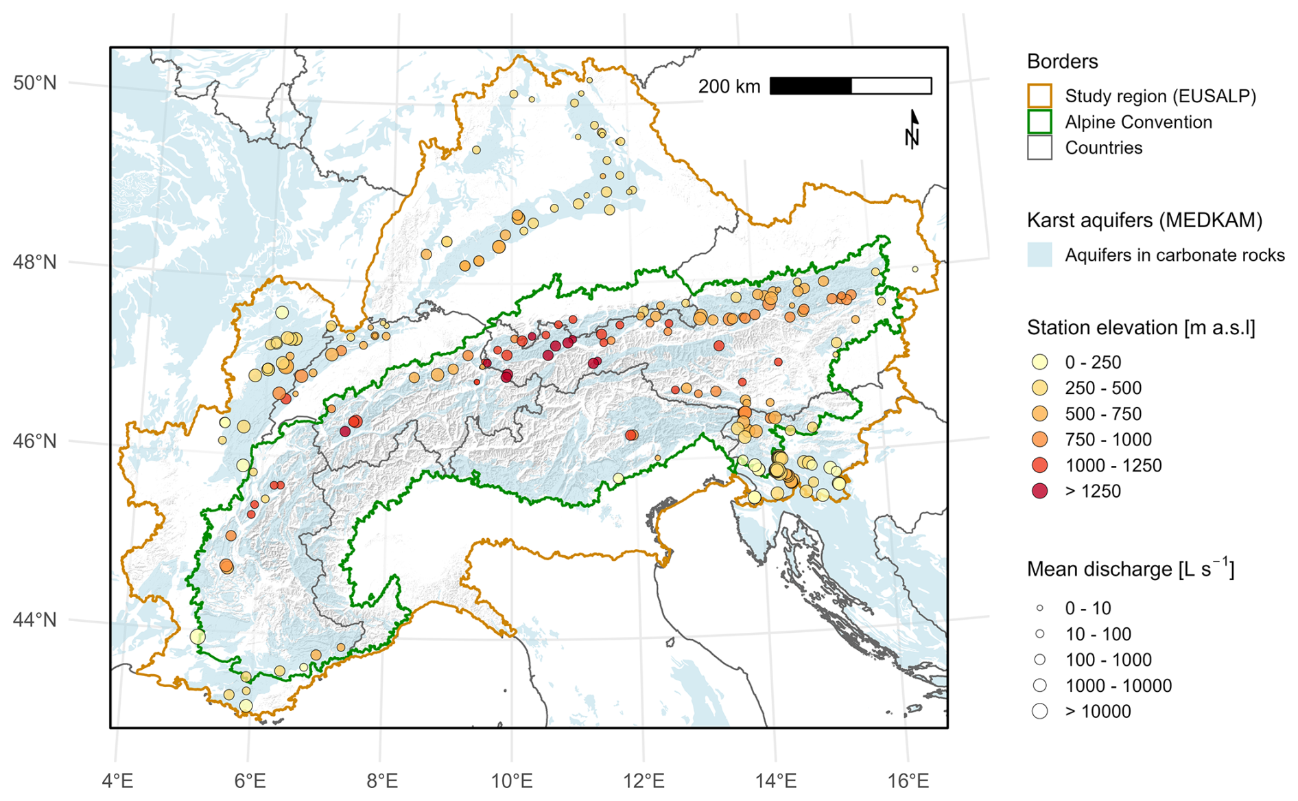
Figure 1Spatial coverage of the ALPAKAS dataset, defined by the EUSALP area, with the core Alpine region delimited by the Alpine Convention. Major karst regions from the MEDKAM dataset and hillshade relief are shown for contextual reference, with national borders indicated by grey lines. ALPAKAS monitoring stations are coloured by elevation and scaled by mean discharge classes. Mean discharge is calculated exclusively across all hydrological years with at least 80 % data availability, as discussed in Sect. 4.3. Administrative borders: © 2018–2025 GADM. Alpine Convention perimeter: Eurac Research and Permanent Secretariat of the Alpine Convention (2025). MEDKAM: Xanke et al. (2022). Hillshade background: Derived from ESA (2023).
Based on the Mediterranean Karst Aquifer Map (MEDKAM; Xanke et al., 2022), approximately 40 % of the core Alpine region and about 29 % of the EUSALP area are covered by karst aquifers, defined in this study as aquifers in sedimentary and metamorphic carbonate rocks. These areas are highlighted in light blue in Fig. 1 and primarily represent carbonate rocks of sedimentary origin, although some have been affected by metamorphic overprinting during Alpine orogenesis. Hydrogeological settings where karst aquifers are possibly present at depth were not considered. The monitoring stations included in ALPAKAS are distributed across eight major structural tectonic units, as shown in Fig. 2c. This classification follows Pfiffner (2009) and comprises the Dinarides, Southern Alps, Eastern Alps, Helvetic units, Penninic units, Jura, European Foreland, and Provence Platform. The distribution of carbonate rocks within the core Alpine region and the corresponding structural tectonic units is described in detail by Goldscheider et al. (2025).
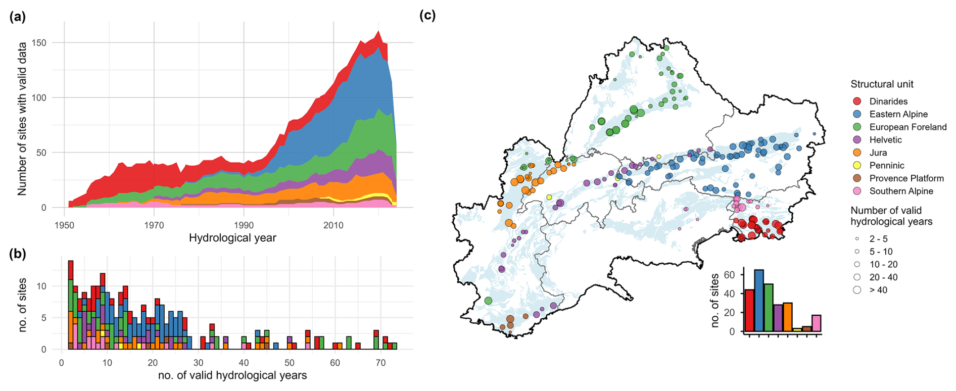
Figure 2Temporal and spatial availability of daily discharge data for all stations included in ALPAKAS, illustrated based on valid hydrological years with respect to E-OBS and ERA5-Land data. Stations are colour coded by structural tectonic units as derived from Pfiffner (2009). (a) Number of sites with valid hydrological years over time. (b) Distribution of the total number of valid hydrological years per station. (c) Spatial distribution of structural tectonic units and the number of valid hydrological years across the dataset. Each point represents a monitoring station, with symbol size scaled according to classes of valid hydrological years. Administrative borders: © 2018–2025 GADM. MEDKAM: Xanke et al. (2022).
Table 1Most important station metadata available in ALPAKAS. Additional station metadata is provided in Table E1.
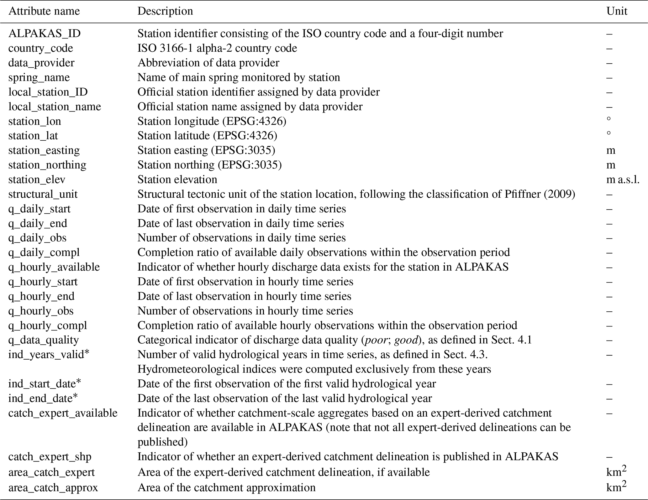
* Variables are provided separately for meteorological products: E-OBS (*_eobs), ERA5-Land (*_era5land) and national datasets (*_nat).
The monitoring stations in ALPAKAS cover a broad range of elevations and discharge magnitudes, which are represented in Fig. 1. Station elevations range from approximately 60 to 1680 m above mean sea level (a.m.s.l.), with a median elevation of 520 m a.m.s.l. Mean discharge varies widely across the dataset, from 0.1 to approximately 23 700 L s−1, with a median value of 285 L s−1.
Table 1 summarizes metadata attributes associated with the spring discharge monitoring stations. For each station, information on the country, data provider, spring name, station coordinates, station elevation as well as on the station name and station ID assigned by the respective data provider is included. In this dataset, the ALPAKAS ID serves as unique identifier and consists of the ISO country code followed by a four-digit number. Additional station metadata are summarized in Table E1 in Appendix E. These variables include information on anthropogenic influences affecting the discharge time series, as well as a wide range of general information related to the station, spring, catchment, and the discharge data itself.
The derivation of catchment-scale variables requires reliable representations of catchment boundaries. In karst systems, however, this is particularly challenging because hydrological boundaries are controlled predominantly by subsurface flow networks rather than by surface topography (Goldscheider and Drew, 2007). Therefore, ALPAKAS includes two alternative catchment representations provided in vector format: (i) expert-based catchment boundaries compiled from public authorities and the literature, where available, and (ii) simplified circular catchment approximations. For the latter, catchment area, i.e. the catchment size, is estimated using a simple local water-balance approach, while topography and available tracer-test information are used to infer the catchment's orientation and position relative to the spring. The catchment approximation approach, as described in Appendix A, builds on the method described by Thinius et al. (2026). It enables the estimation of catchment-scale variables for springs lacking well-defined catchment boundaries and was applied to all monitoring stations.
The station metadata indicate for each station whether catchment-scale aggregates based on an expert-derived delineation are available, whether the corresponding shapefile is published within the dataset, and include the areas of both expert-based and approximated catchments (Table 1). In total, the dataset comprises expert-based catchment aggregates for 151 springs, while the associated catchment geometries could only be included for 105 springs due to licensing restrictions. Details on catchment delineation, including data citations and delineation methods applied, are provided directly in the expert catchment delineation file, whereas the catchment approximation file documents the tracer data sources and the number of tracer tests used to determine the placement of the approximated catchment relative to the spring. While the quality of expert-based catchment delineations can vary considerably depending on data availability and applied methods, circular catchment approximations are generally more uncertain and may differ substantially from delineated catchments. Consequently, variables derived from approximated catchment representations should be interpreted with caution. A detailed description of the methodology used for the simplified catchment approximations is provided in Appendix A.
All catchment-scale variables in ALPAKAS were derived by aggregating spatially distributed information within each catchment representation using area-weighted arithmetic means. This approach was applied consistently to derive the meteorological time series and the static catchment attributes. For raster-based products, aggregation was performed using the exact_extract function of the exactextractr R package (Baston, 2025), which accounts for the exact fractional overlap between raster cells and catchment polygons. This was considered particularly important for small catchments, where partial cell coverage can otherwise introduce substantial aggregation bias. While this approach minimizes aggregation uncertainty associated with partially covered raster cells, other uncertainties in catchment-scale estimates remain, as further discussed in Sect. 6.2. Although some spatial detail is inevitably lost through aggregation of distributed data products, catchment attributes offer a coherent and comparable representation of catchment characteristics suitable for data-driven modelling and cross-catchment analyses (Addor et al., 2017). The comprehensive selection of static attributes is further intended to support data-driven modelling approaches, allowing models to explore the relevance of different catchment characteristics across Alpine karst springs. Spatial analyses and mapping within ALPAKAS were conducted using the ETRS89-LAEA Europe coordinate reference system (EPSG:3035) to ensure accurate area representation across the dataset’s spatial coverage.
All timestamps are reported in UTC+01 which corresponds to CET (winter time). Hourly data mark the beginning of the interval, such that the indexed hour denotes the period from the stated hour to the subsequent hour (HH = (HH):00–(HH+01):00). An overview of the hydrometeorological time series available in ALPAKAS is provided in Table D1 in Appendix D.
4.1 Discharge data
ALPAKAS comprises karst spring hydrographs obtained from public authorities, scientific monitoring networks and individual researchers across all seven countries of the EUSALP region. The dataset contains both daily and hourly karst spring discharge time series, which were subjected to a uniform preprocessing workflow. The observational data originate from national authorities (ARSO, 2020; AU, 2025; BAFU, 2025a, b; BMLUK, 2025; SCHAPI, 2022), regional authorities (AfU, 2025; ARPAV, 2025; AWA, 2025; Conthey, 2025; DGE, 2025; LfU, 2025; LUBW, 2025; Savoie, 2025), and several research projects and research observation networks (Baudement et al., 2017; Bittner et al., 2018; Dirnböck, 2020; Epting et al., 2018; Jeannin et al., 2021; Olarinoye et al., 2020; SNO KARST, 2025a, b, c).
To ensure consistent data handling, all received discharge time series were standardized prior to preprocessing using R, including harmonization of date formats and conversion of discharge units to L s−1. The obtained data comprise three temporal resolution classes: (a) daily, (b) hourly, and (c) instantaneous observations (i.e. provider-specific sub-hourly records). Preprocessing steps were applied conditionally based on the original temporal resolution, following the workflow presented in Fig. B1 in Appendix B. In general, the highest resolution available from each data provider was used and subsequently aggregated to hourly and daily time series, as described in detail in Appendix B3. For some providers, however, additional daily time series were included when they contained information not available in the higher-resolution records. The original temporal resolution of each time series is documented in the station metadata (Table E1). Where both were available, comparisons between daily values derived through aggregation of higher-resolution data and those provided directly by data providers showed only minimal differences.
Beyond temporal resolution, the time series differed in data quality, underlying measurement infrastructure, applied methods, and prior internal data processing practices. To achieve a consistent level of data harmonization across the dataset, a uniform preprocessing workflow was implemented, while explicitly accounting for the substantial variability in hydrograph dynamics between individual karst systems. This preprocessing comprised the identification of outliers and artefacts using a combination of manual and automated procedures and the annotation of the time series with various quality flags. Depending on the original temporal resolution, the data were aggregated to hourly and daily time steps. For daily and hourly resolutions, identified outliers were retained as flagged observations, allowing evaluation of the quality-control procedure. For instantaneous time series requiring aggregation to hourly values, flagged outliers and artefacts cannot be traced in the aggregated time series, as they were removed prior to aggregation. Additional flags describing resolution and quality of individual time series segments were assigned to facilitate flexible and efficient data subsetting. Finally, a conservative changepoint detection was applied to identify sustained shifts in the mean or variance of the discharge time series, as described in detail in Appendix B4. Detected changepoints as well as the segment considered most reliable were flagged to support the identification of affected time series sections. The preprocessing procedure implemented in R is described in more detail in Appendix B.
Missing values in discharge time series of ALPAKAS were neither interpolated nor imputed. This decision is motivated by the highly dynamic nature of many karst spring hydrographs, for which the filling of larger gaps requires the incorporation of precipitation data. As the dataset is also intended for machine learning applications, such gap filling could introduce data leakage, since imputation commonly exploit future information and may therefore provide models with information unavailable at prediction time, violating temporal causality. Consequently, the treatment of missing values is deliberately left to the users of the dataset, allowing them to apply methods appropriate to their specific use cases. It should be noted that the spring hydrographs were preprocessed by the data providers to varying extents, while detailed documentation of the applied preprocessing steps is often unavailable. As part of the harmonization effort to achieve a more uniform data quality across the dataset, linear segments spanning several weeks and indicative of interpolation were identified and flagged in the discharge time series.
Owing to the strongly heterogeneous temporal coverage of individual time series, no common reference period was defined. For each station, the full available record up to the end of 2024 was included in the dataset to support flexible use. During preprocessing, isolated observations and periods with coarser temporal resolution than the target resolution were retained rather than removed, as they may provide valuable information. These segments were flagged accordingly, enabling straightforward subsetting by temporal resolution class (Appendix B4).
For both daily and hourly resolutions, the start and end dates of the discharge time series, the total number of available observations, and the completion ratio are provided in the station-related metadata (Table 1). The completion ratio was calculated as the number of available observations, including flagged observations, divided by the total number of time steps between the first and last observation. The metadata further include a categorical quality indicator that groups time series based on their overall appearance. Only six stations were classified as poor due to poor effective measurement resolution, pronounced noise, or implausible hydrograph shapes. In this dataset, multiple stations can be associated with a single karst spring. In most cases, these stations represent measurements of the same spring at nearby locations during different time periods and were retained as separate time series rather than combined into a single discharge record. In some cases, however, a downstream station may also include discharge contributions from additional springs. Associated stations are indicated in the metadata by providing the station identifiers of the corresponding upstream and downstream stations (Table E1).
While ALPAKAS focuses on spring discharge, the availability of complementary water-quality data and the possible future extension of ALPAKAS is briefly discussed in Appendix C.
4.2 Meteorological data
ALPAKAS contains precipitation and temperature time series derived from multiple meteorological data products spanning global, continental, and national scales. By focusing on dynamic variables for which future projections exist, we support scenario-based analyses. Because these data are obtained from continuous gridded products, the meteorological time series are gap-free. Meteorological catchment aggregates are provided for each station over the full period covered by the meteorological dataset through the end of 2024, independent of availability of discharge observations.
Cornes et al. (2018)Muñoz Sabater (2019a)GeoSphere Austria (2020)MeteoSwiss (2024a, b, c, d)DWD (2025a, b, c, d)Vidal et al. (2010)Škrk et al. (2020)Table 2Summary of daily meteorological data products and variables included in ALPAKAS.
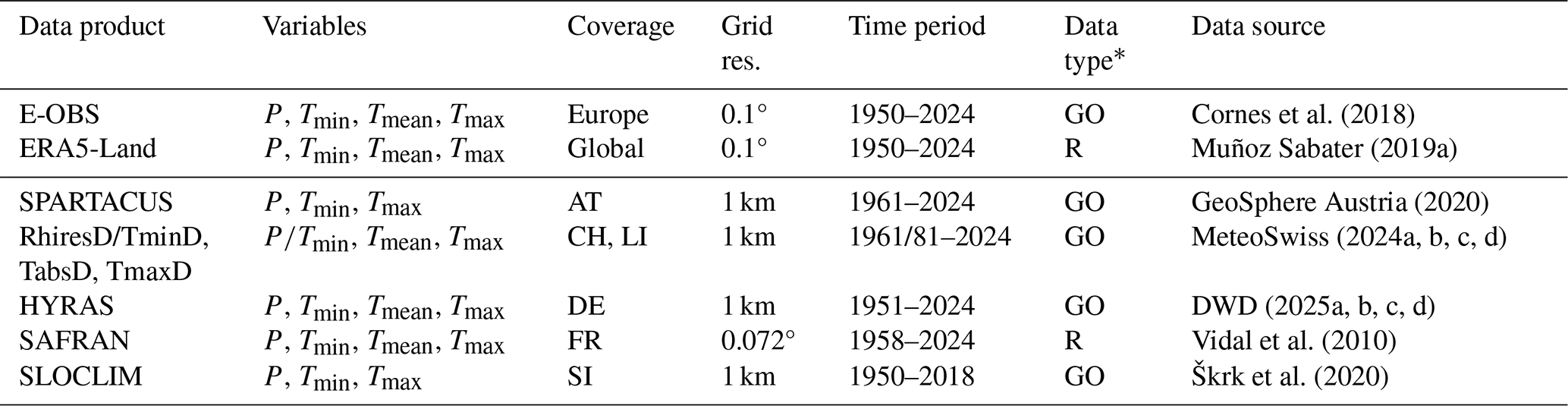
* GO = Ground observations; R = Reanalysis.
For each monitoring station with an hourly discharge record, hourly precipitation and mean temperature are provided based on ERA5-Land reanalysis data (Muñoz Sabater, 2019a). Daily meteorological data products included in ALPAKAS are summarized in Table 2, which highlights differences in spatial coverage, grid resolution, temporal extent, and data type. ERA5-Land is produced by the European Centre for Medium-Range Weather Forecasts (ECMWF) using a land surface model driven by ERA5 atmospheric forcing. Daily ERA5-Land time series were derived from the hourly data, with minimum and maximum temperatures defined by the corresponding hourly extremes. E-OBS is a daily observation-based gridded dataset derived by interpolating quality-controlled station observations from the European Climate Assessment & Dataset (ECA&D). Together, E-OBS and ERA5-Land provide a consistent long-term daily baseline at 0.1° spatial resolution across the entire dataset's spatial coverage. For both products, ALPAKAS includes precipitation as well as minimum, mean, and maximum temperature from 1950 onward, enabling homogeneous derivation of meteorological attributes across national boundaries. In contrast to the region-wide datasets, national meteorological data products offer substantially higher spatial detail. Observation-based products at 1 km grid resolution are available for Austria (SPARTACUS; GeoSphere Austria, 2020), Switzerland and Liechtenstein (RhiresD, TminD, TabsD, TmaxD; MeteoSwiss, 2024a, b, c, d), Germany (HYRAS; DWD, 2025a, b, c, d), and Slovenia (SLOCLIM; Škrk et al., 2020). For France, daily meteorological fields from the SAFRAN reanalysis (Vidal et al., 2010) at a spatial resolution of 0.072° were used, with rainfall and snowfall summed to derive total precipitation. While these national products capture regional climatic variability in greater detail, they differ in temporal coverage and in the availability of temperature variables, which should be considered when comparing meteorology-based attributes across product classes. In particular, SPARTACUS and SLOCLIM do not provide daily mean temperature, and SLOCLIM is only available until 2018.
The accumulation period of daily precipitation in the national meteorological data products typically spans from 06:00 to 06:00 local time, whereas ERA5-Land daily data are accumulated over the calendar day from 00:00 to 24:00 UTC. For E-OBS, it is explicitly stated that the exact accumulation periods may vary among the contributing data providers. Consequently, the differences in accumulation periods can lead to small temporal mismatches between precipitation and discharge data for some products, which should be considered during analysis.
4.3 Data availability by valid hydrological years
To prevent systematic biases arising from incomplete or seasonally uneven records (e.g., an increased frequency of missing values during winter months) and to ensure comparability of meteorological and hydrological indices, static attributes derived from meteorological and discharge data were evaluated only for hydrological years with data available for at least 80 % of calendar days in both records (hereafter referred to as valid hydrological years). A common hydrological year definition spanning from 1 October to 30 September was adopted consistently across the dataset, following the convention commonly used in Austria and Switzerland, as it generally captures a complete snow accumulation and melt cycle also for higher-elevation catchments in the Alps. As the meteorological data are derived from continuous gridded products, data availability was primarily constrained by the discharge observations. Only stations with at least two valid hydrological years were retained in ALPAKAS. For each meteorological data product class, the start date, end date, and the total number of valid hydrological years are provided in the station metadata (Table 1).
Figure 2 provides an overview of the temporal and spatial availability of valid hydrological years for karst spring discharge data in ALPAKAS with respect to the E-OBS and ERA5-Land meteorological data. Data availability is presented by major structural tectonic units of the wider Alpine region, as defined by Pfiffner (2009) and provided in the station metadata (Table 1), enabling an assessment independent of national boundaries and the large number of contributing data providers. Figure 2a illustrates the temporal distribution of valid hydrological years across ALPAKAS. The first valid hydrological year is 1951, reflecting the onset of the E-OBS and ERA5-Land meteorological data. Only a few discharge time series from Slovenia extend further back in time, with the earliest record beginning in 1924. Data availability remains relatively stable until the mid-1990s, albeit with varying regional contributions and a decreasing dominance of records from the Dinarides. From the mid-1990s onward, the number of time series containing valid hydrological years increases markedly. Between 2015 and 2022, data availability reaches a plateau, with over 60 % of all time series in the dataset containing valid hydrological years and a maximum of 161 stations in 2020. The apparent decline after 2022 is solely attributable to delays in data reporting by some providers at the time of data acquisition. Figure 2b shows the distribution of the total number of valid hydrological years per site, which ranges from 2 to 73, with a median of 14. Figure 2c illustrates the spatial distribution of valid hydrological years in relation to structural tectonic units across the dataset. Data availability varies substantially across the EUSALP region, with most sites (65) located within the Eastern Alps, whereas only three and five sites are situated within the Penninic units and Provence Platform, respectively.
5.1 Topography and Positioning
By controlling meteorological forcing and reflecting physiographic characteristics (Addor et al., 2017), catchment elevation exerts a key control on processes influencing karst spring discharge. To characterize topographic variability, a set of elevation statistics (minimum, mean, median, maximum, 10th, 25th, 50th, 75th and 90th percentiles) was derived from the Copernicus GLO-30 digital elevation model (GLO-30) at 30 m grid resolution (ESA, 2023). Mean slope and mean aspect, represented by its northness and eastness components to account for the circular nature of aspect, were derived from the corresponding precomputed products provided by the European Space Agency. To obtain a meaningful aspect metric, aspect values were weighted by the sine of the slope angle, thereby reducing the influence of nearly flat areas that lack a dominant orientation (Amatulli et al., 2018). In addition, the proportions of flat terrain (slope <3°) and steep terrain (slope >15°) were included following the CAMELS-CH dataset (Höge et al., 2023).
Drainage density was calculated as the ratio of the total length of all stream segments within the catchment boundaries to the catchment area (Horton, 1932) and was considered a potential proxy for the degree of karstification. Stream networks were extracted from the EU-Hydro River Network Database (EU-Hydro; EEA, 2019). In addition, positional attributes describing station location with respect to the Thiessen catchment and the river network of Strahler stream orders 1 and 2 were derived from the Multiorder hydrologic Position for Europe (EU-MOHP) dataset (Nölscher et al., 2022) at 30 m grid resolution. Climate zones at station locations were extracted from Beck et al. (2023) following the Köppen-Geiger climate classification. Topographic and positional attributes are listed in Table E2.
5.2 Meteorology and hydrology
Hydrometeorological indices (Table E3) were derived based on the preprocessed daily dataset after the removal of outliers, artefacts, and unreliable time series segments identified through changepoint analysis (Sect. 4.1). The meterorological variables in this dataset represent spatially aggregated catchment-scale values, as described in Sect. 3. Both attribute classes were calculated exclusively for valid hydrological years to prevent systematic biases and to ensure the comparability of hydrological and meteorological indices (Sect. 4.3). All indicators incorporating meteorological variables were computed independently for each meteorological data product class. Hydrological indicators relying solely on discharge data were calculated for valid hydrological years with respect to the coverage of E-OBS and ERA5-Land.
Meteorological indices were closely aligned with the climatic attributes used in the CAMELS datasets. In addition to mean daily precipitation, indicators of precipitation seasonality and extreme precipitation events, as well as the fraction of precipitation falling as snow, were computed following the original CAMELS dataset (Addor et al., 2017). The calculation of extreme precipitation events was adapted to allow analysis across segments of valid hydrological years separated by missing years, with segment-wise estimates subsequently averaged. In addition, mean daily temperature, hydrological-year mean daily minimum and maximum temperature, and the frequency of days with mean temperature ≤0 °C were computed following Wood et al. (2025). For consistency, mean daily temperature used in the calculation of snow fraction was defined as the average of daily minimum and maximum temperature. Figure 3 illustrates the spatial distributions of selected meteorological indices for the monitoring stations included in ALPAKAS, computed from E-OBS data using the approximated catchments. While discussion and interpretation remain beyond the scope of this study, the figure reveals spatial patterns and correlations that highlight the potential of the dataset for further analyses.
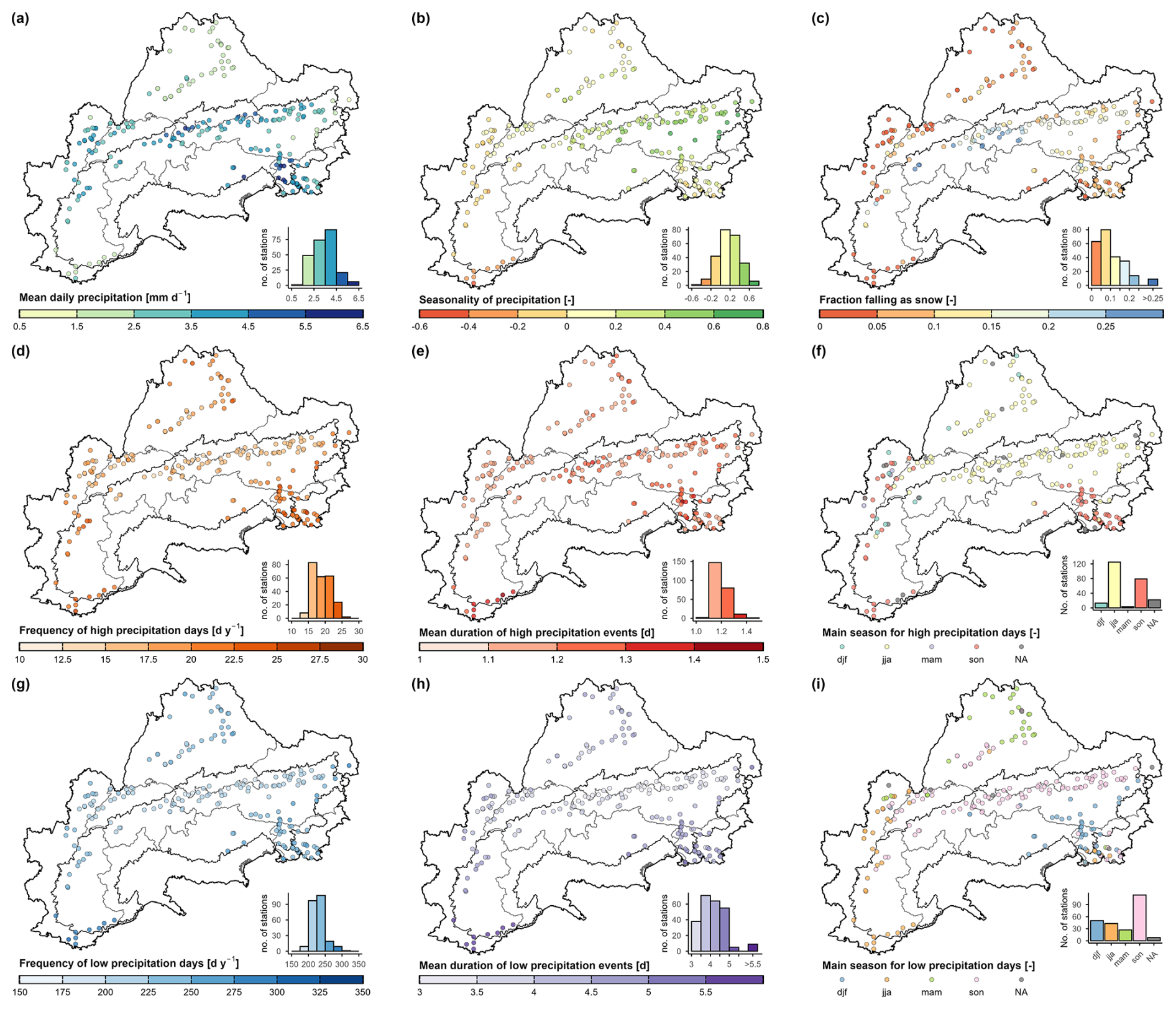
Figure 3Spatial distributions of selected meteorological indices (Table E3) computed based on the catchment approximations using E-OBS. The overall distributions of the respective attributes are shown by accompanying histograms. Administrative borders: © 2018–2025 GADM. Alpine Convention perimeter: Eurac Research and Permanent Secretariat of the Alpine Convention (2025).
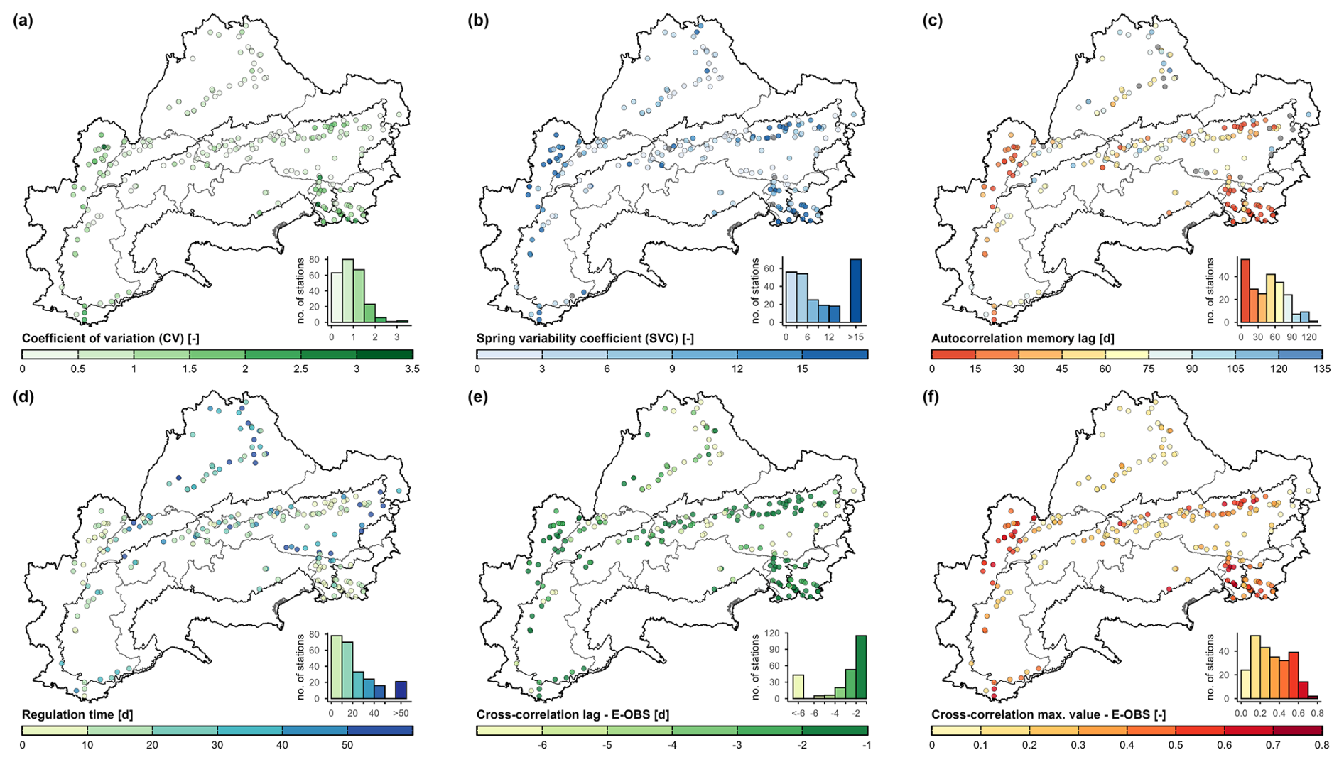
Figure 4Spatial distributions of selected hydrological indices (Table E3) computed based on the catchment approximations using E-OBS to compute cross-correlation. The overall distributions of the respective attributes are shown by accompanying histograms. Administrative borders: © 2018–2025 GADM. Alpine Convention perimeter: Eurac Research and Permanent Secretariat of the Alpine Convention (2025).
In addition to descriptive statistics of the discharge time series following Cinkus et al. (2023) (minimum, mean, maximum, 10th and 90th percentiles, and standard deviation), variability indices commonly used in karst hydrology were computed, including the coefficient of variation and the spring variability coefficient (Flora, 2004). Discharge-based hydrological indicators were reported in volumetric units rather than normalized by catchment area to avoid directly propagating uncertainty associated with alternative catchment delineations into the derived indicators. To further characterize the hydrodynamic behaviour of the karst systems, temporal dependence was analyzed using autocorrelation of the discharge time series and cross-correlation between precipitation and discharge, computed with the stats package in R. Prior to the analysis, data gaps of up to five days were interpolated using a monotone Hermite spline from the zoo package (Zeileis and Grothendieck, 2005), as suggested by Cinkus et al. (2023). Following Mangin (1984), autocorrelation was computed with a maximum time lag of 125 d, while the memory effect was defined as the first time lag at which the autocorrelation function decreases to a value of 0.2. For the cross-correlation analysis, both the maximum correlation coefficient and the corresponding lag were derived using a maximum lag of 100. Because the computation of regulation time based on spectral analysis requires continuous discharge records, the regulation time was approximated based on the standard deviation σ using the ratio σ250σ−1, as proposed by Bailly-Comte et al. (2023) and implemented into the XLKarst Excel tool. This metric is derived from the standard deviation of discharge within a moving window of 250 d. As the discharge time series contain gaps and entirely missing hydrological years, only windows with at least 80 % data availability were retained. This constraint avoids a disproportionate influence of data points adjacent to large gaps on σ250, which could otherwise lead to a systematic distortion of the metric. The spatial distributions of selected hydrological indices are shown in Fig. 4. These indices display a much more spatially heterogeneous pattern than the meteorological indices (Fig. 3), mainly reflecting the control exerted by the individual karst systems.
5.3 Land cover and glacier
Land cover attributes were derived from the CORINE Land Cover (CLC) 2018 raster dataset (EEA, 2020) at 100 m spatial resolution, provided by the European Environment Agency (EEA) through the Copernicus Land Monitoring Service. CLC products are updated on a six-year cycle and are consistently available for the full spatial coverage of the dataset only from 2000 onward. The most recent dataset, CLC 2018, was selected as it offers the highest mapping accuracy and constitutes an appropriate intermediate reference point between historical land use conditions and those relevant for future scenario analyses. CLC 2018 is primarily based on Sentinel-2 (10 m resolution) and Landsat-8 (30 m resolution) satellite imagery and contains 44 land use classes. For ALPAKAS, land cover percentages per catchment were derived adopting the twelve categories defined in CAMELS-CH (Höge et al., 2023): crop, grass and herb vegetation, shrub vegetation, forest (coniferous, deciduous and mixed), wetland, ice and perpetual snow, inland water surface, rock (loose and solid) and settlements/urban (Table E4). These categories were defined to capture the highly heterogeneous Alpine topography, which is also of central importance for our analysis.
The land cover class ice and perpetual snow was complemented with more reliable glacier outlines providing temporally explicit snapshots of glacier coverage within each catchment, as also reported in Table E4. Glacier cover percentages for 2003 were derived from the Randolph Glacier Inventory (RGI Consortium, 2023), which for the Alpine region incorporates Landsat-based outlines at 30 m mapping resolution from Paul et al. (2011). Glacier cover percentages for 2015 were obtained from the pan-European glacier inventory by Paul et al. (2019, 2020), which provides higher-accuracy outlines at 10 m mapping resolution based on Sentinel-2 data and earlier glacier inventories. In addition, glacier fractions for 1850 were derived from reconstructed outlines compiled by Reinthaler (2024) through geomorphological interpretations and historical topographic maps. We acknowledge that more reliable and temporally continuous glacier datasets exist for individual countries within the dataset's spatial coverage. In addition to glacier area, the Swiss Glacier Monitoring Network GLAMOS (Linsbauer et al., 2021) provides high-resolution data on glacier volume, which is particularly useful for modelling glacier storage processes. However, this study focuses on catchment attributes derived from data products that cover the full spatial extend of ALPAKAS to maintain spatial consistency and comparability.
5.4 Soil
Soil attributes (Table E5) at catchment scale were primarily derived from the European Soil Database Derived (ESDD) dataset (Hiederer, 2013a, b) provided by the European Soil Data Centre (ESDAC). The dataset has a spatial resolution of 1 km and is based on harmonized national and regional soil information compiled in the European Soil Database (ESDB). Topsoil and subsoil layer values were generally aggregated using depth-weighted averages, whereas total available water content was calculated by summing layer values.
This information was complemented with soil porosity and saturated hydraulic conductivity from the 3D Soil Hydraulic Database of Europe (EU-SHD; Tóth et al., 2017) at 250 m spatial resolution. EU-SHD is derived from the SoilGrids database (Hengl et al., 2017) using pedotransfer functions and is provided at the six standard SoilGrids depth intervals. These variables were aggregated using weights corresponding to the respective depth intervals. Since SoilGrids relies on a global machine learning approach trained on datasets with strong representation from the United States, these variables should be interpreted with caution for the complex soil patterns in the Alpine region.
As an additional attribute, depth to bedrock was derived from the Global 1 km Gridded Thickness of Soil, Regolith, and Sedimentary Deposit Layers (GGT) dataset (Pelletier et al., 2016) at approximately 1 km spatial resolution. This dataset provides the estimated thickness of unconsolidated and weathered material above bedrock and is calibrated using borehole profiles primarily from the USA and Europe. As with the other global products, the derived attributes should be interpreted cautiously, particularly in regions with complex topography such as the Alps.
5.5 Hydrogeology
Hydrogeological attributes (Table E6) were primarily derived from the International Hydrogeological Map of Europe 1 : 1 500 000 (IHME1500; BGR and UNESCO, 2019), provided by the Federal Institute for Geosciences and Natural Resources (BGR). IHME1500 comprises harmonized pan-European hydrogeological information compiled from national contributions and expert interpretation and is organized within a multi-level lithological classification with five levels of detail. For ALPAKAS, the ten petrographic groups of lithology level 4 were used. The karst related level 1 classes limestones (jointed, karstified); dolomitic limestones (jointed, karstified); and chalkstones, limestones (jointed, karstified) were additionally extracted, as they are of particular interest for this dataset. Catchment-scale aggregates are also computed for the six IHME1500 aquifer productivity classes, ranging from highly productive aquifers to practically non-aquifer formations. These classes follow the Standard Legend for Hydrogeological Maps (SLHyM) and represent expert-based regional assessments of groundwater productivity based on lithology, porosity type, and degree of fracturing or karstification.
To refine the representation of karst systems, the attributes karst aquifers in sedimentary and metamorphic carbonate rocks, karst aquifer possibly present at depth, and non-karst aquifers were further derived from the Mediterranean Karst Aquifer Map (MEDKAM; Xanke et al., 2022). The MEDKAM class karst aquifers in evaporite rocks is not present within the project area. MEDKAM provides a regional compilation of karst aquifers at 1 : 5 000 000 scale and is based largely on IHME1500 and additional national information, following the mapping approach of the World Karst Aquifer Map (WOKAM; Chen et al., 2017).
For both IHME1500 and MEDKAM, catchment-scale attributes were derived from the areal proportions of hydrogeological classes within each catchment representation. Given the relatively coarse map scales, these attributes provide a generalized characterization of catchment hydrogeology, while local heterogeneity may not be accurately represented, particularly in small catchments. These uncertainties are further discussed in Sect. 6.2. However, even high-resolution regional maps typically fail to capture the heterogeneous and often conduit-dominated hydraulics of karst systems. Therefore, the hydrogeological attributes were complemented with hydrological indices directly derived from the hydrographs to better characterize the karst systems in this dataset (Sect. 5.2). Table E1 also includes WOKAM, MEDKAM and WOKAS identifiers, as well as an indicator of whether a spring is listed among the globally important karst springs of the MIKAS project (Stevanović, 2023), facilitating access to related information.
6.1 Uncertainties in discharge data
The accuracy of spring discharge data can vary substantially depending on the measurement infrastructure, applied methods, and prior internal data processing practices. In many cases, initial quality control is performed and missing data may be interpolated by the respective data provider, but detailed documentation of the applied processing steps is often lacking. Spring discharge is typically monitored by recording hydrostatic pressure using submerged pressure sensors, from which water level and, subsequently, discharge are inferred using empirically derived rating curves. Sensor calibration and rating curves are a common source of uncertainty, especially for extreme hydrological events (Westerberg et al., 2022). Additional sources of uncertainty include site or instrument changes, irregular or inadequate instrument maintenance, anthropogenic influences, and temporal changes in channel controls (Wilby et al., 2017; Strohmenger et al., 2023).
Discharge uncertainties arising from stage-discharge relationships can vary substantially between monitoring stations and across flow conditions. Focusing specifically on karst springs and rivers, Jeannin et al. (2026) analyzed 16 Swiss monitoring stations, of which eight are also included in ALPAKAS. They estimated relative uncertainties of approximately 5 % for flow conditions occurring around 60 % of the time, but substantially higher uncertainties of around 30 % during high-water conditions and at least 50 % during low-water conditions, sometimes approaching 100 %. This strong variation partly reflects the wide discharge ranges typical of karst springs, which can be difficult to measure accurately with a single-stage weir. To reduce uncertainties at extreme flows while maintaining generally low uncertainty, Jeannin et al. (2026) recommend compound weirs with two or three stages. However, these estimates depend strongly on individual station characteristics and cannot be directly transferred to ALPAKAS. The importance of station-specific assessments is also illustrated by CAMELS-GB (Coxon et al., 2020), where rating-curve-related discharge uncertainty was quantified for 503 gauging stations based on an existing dataset of rating curves and stage-discharge measurements. Comparable quantitative uncertainty assessments for ALPAKAS would require detailed station-specific information on measurement methods, rating curves, and gauging infrastructure, which is not consistently available across the different data providers.
Beyond uncertainties in discharge measurements, karst systems often discharge through multiple outlets rather than a single spring. For example, intermittent overflow springs may become active only during major precipitation events and part of the discharge may bypass the station through subsurface flow, with relatively larger contributions during low-flow conditions (Jeannin et al., 2026). Monitoring stations located further downstream may capture a larger proportion of the total outflow of the karst system, but may also include additional contributions from surface runoff, as indicated in ALPAKAS. This uncertainty is not directly associated with the hydrograph itself but rather with how well the monitored discharge represents the total outflow of the karst system and its associated catchment.
Consistent quality control of karst spring discharge remains particularly challenging owing to the high heterogeneity and dynamic flow conditions typical of karst systems. While the uncertainties associated with discharge measurements persist through data preprocessing, ALPAKAS seeks to improve data quality and consistency through an extensive and conservative preprocessing procedure uniformly applied to all time series (Fig. B1), with the aim of providing a dataset of daily and hourly quality-controlled and harmonized spring discharge records. While visual inspection of hydrographs introduces subjectivity and reduces reproducibility, it remains a recommended component of hydrological data quality assessment (Barthel et al., 2022) and was therefore applied in combination with automated procedures. Accordingly, preprocessing involved the identification of outliers through a combination of manual inspection and automated methods, as well as the detection of plateaus caused by sensor cut-offs, abrupt step changes, interpolated segments, and periods of elevated noise. Outliers and artefacts were flagged rather than removed to assure reproducibility and to allow users to independently assess the identified features. Additional quality and resolution flags are provided to enable straightforward subsetting of the time series. These flags allow users to exclude isolated observations, periods of reduced effective measurement resolution or increased noise, and changepoints indicative for implausible behaviour, such as anthropogenic influence or station renewal. Where available, station metadata (Table E1) further document the influence of surface water contributions and water extraction for drinking water supply or hydropower production, as well as the measurement methods and instruments employed. The metadata also include documentation of data related issues, such as periods of unreliable measurements, station renewals, or station relocations.
Temporal resolutions of discharge time series in the dataset are heterogeneous and may change within individual records as a result of implementation of more modern measurement techniques. Minor uncertainty may be introduced when resampling higher resolution data to hourly and daily time series using time-weighted aggregation. In contrast, substantially greater uncertainty is expected for some discharge records originating from pseudo-highly resolved time series with low effective measurement resolution. Restricting the calculation of hydrometeorological indices to valid hydrological years reduces systematic biases caused by disproportionate seasonal representation. Nevertheless, major discharge events may be poorly captured or missing in some time series due to damage or failure of measurement infrastructure, or because observed stages exceed the calibrated range of rating curves, potentially introducing systematic biases.
6.2 Uncertainties in catchment-scale variables
Catchment representations constitute a major source of uncertainty in this dataset, as catchment-scale variables critically depend on their spatial definition and catchments are particularly difficult to derive for karst springs (Ford and Williams, 2007). Accordingly, ALPAKAS clearly distinguishes between delineated catchments, for which information on the data provider and delineation methods is provided, and circular catchment approximations, which serve as a pragmatic alternative where delineated catchments are unavailable (Appendix A). Uncertainties associated with the catchment approximations are discussed in detail by Thinius et al. (2026). Additional uncertainty arises from the aggregation method applied to derive catchment-scale variables from distributed data products (Sect. 3), which inevitably reduces spatial detail and may smooth local variability.
Owing to the large number of meteorological and static catchment attributes included in ALPAKAS, a detailed discussion of uncertainties associated with individual data products from which the catchment-scale variables are derived is beyond the scope of this study, and uncertainties may vary considerably within and between catchments. Instead, this section discusses general considerations relevant to the interpretation of these attributes. In general, it should be recognized that the effective resolution of aggregated catchment variables may differ substantially from the nominal grid resolution of the underlying data products.
Uncertainties in data products used to derive static catchment attributes primarily arises from the quality of the input data, scale and resolution mismatch, spatial generalisation that limits the accurate representation of locally heterogeneous characteristics, and assumptions inherent in model-derived products.
Similar to the products used for static catchment attributes, uncertainties in observation based meteorological products (Table 2) primarily arise from measurement errors, heterogeneous station density, and the spatial interpolation of station data used to generate gridded fields, which can smooth local variability and dampen extremes (Cornes et al., 2018). Additional uncertainty stems from temporal inhomogeneities related to changes in instruments, station locations, or observing practices (Bongiovanni et al., 2025), which can have pronounced effects at the catchment scale, particularly given the long time periods covered by the data included in ALPAKAS. As reanalysis data are generated by assimilating observations into numerical weather models, uncertainties inherent to observation based products generally also apply and propagate through the assimilation process. In addition, reanalysis meteorological products are subject to uncertainties related to model structure and parameterisation, limitations in data assimilation, and the representation of physical processes. Both observational and reanalysis data may exhibit biases particularly in precipitation, with pronounced effects in data sparse regions and in areas of complex topography such as the Alps (Bongiovanni et al., 2025). The magnitude of these uncertainties varies substantially between meteorological variables, products, temporal scales, and catchments. For example, Wood et al. (2025) evaluated several reanalysis products, including ERA5-Land, across 97 Swiss headwater catchments and reported median biases in mean annual precipitation of approximately 0 %–20 % relative to gridded observations, depending on the product, while corresponding temperature biases were generally below 1 °C. Substantially larger biases occurred for individual catchments and extreme conditions. However, such comparisons are also affected by uncertainties in the gridded observational reference data. For some observation-based meteorological products, spatially and temporally resolved uncertainty estimates are provided, including ensemble-based estimates for E-OBS (Cornes et al., 2018) and model-based prediction uncertainty for SLOCLIM (Škrk et al., 2020). However, comparable uncertainty information is not consistently available across all products, and a comprehensive quantitative assessment at the catchment-scale would require product-specific evaluations and suitable reference data, highlighting an important direction for future work. Further information on uncertainties specific to individual meteorological products are described in the respective dataset documentations accompanying each product (Table 2).
Beyond uncertainties in the provided catchment-scale variables, an additional limitation is the absence of dynamic variables related to snow cover and evapotranspiration. Both play important roles in controlling karst spring discharge in Alpine catchments. Their absence may therefore constrain hydrological interpretation and require additional preprocessing, such as the implementation of snow and evapotranspiration routines, for hydrological modelling applications.
The ALPAKAS dataset is freely available via Zenodo at https://doi.org/10.5281/zenodo.19329693 (Joger et al., 2026) under an open-access license. It follows the FAIR principles (Wilkinson et al., 2016) and is accompanied by comprehensive documentation. All code used for dataset processing was implemented in R and is publicly available in a dedicated code repository archived on Zenodo at https://doi.org/10.5281/zenodo.24159190 (Joger and Thinius, 2026), including documentation for reproducibility. R package dependencies are managed and documented using the renv package (Ushey and Wickham, 2026).
Standardized large-sample benchmark datasets play an increasingly important role in enabling comparative and data-driven research. ALPAKAS addresses this need by integrating 242 daily and 182 hourly quality-controlled and harmonized karst spring discharge hydrographs for the wider Alpine region from more than 20 different providers. It is complemented by catchment representations and a comprehensive set of catchment-scale variables, derived from existing delineations for 151 springs and supplemented by a simple catchment approximation approach that provides catchment aggregates for all stations. As the first large-sample dataset specifically targeting Alpine karst springs, ALPAKAS offers several distinctive features, including the integration of multiple meteorological products at different spatial scales and the provision of hourly time series where available.
By providing a consistent and transparent data basis, ALPAKAS creates new opportunities for comparative analyses, benchmarking of process-based and data-driven models, and more robust assessments of hydrogeological processes and climate change impacts affecting Alpine karst springs. Its structure is aligned with the widely used CAMELS framework, supporting compatibility with established large-sample hydrology workflows. By reducing the need for individual data harmonization and preprocessing, it facilitates more efficient and reproducible research. More systematic assessments and documentation of discharge uncertainty by monitoring agencies would support future efforts to quantify uncertainties in ALPAKAS, for example through station-specific, flow-dependent uncertainty classes assigned to individual observations. Similarly, incorporating additional dynamic catchment variables influencing Alpine karst spring discharge, particularly snow-related variables and evapotranspiration, would be a valuable future extension. More broadly, owing to its open and extensible design, ALPAKAS can be expanded to include additional spring discharge monitoring stations, water-quality data, further catchment-scale variables, karst-specific indices, and climate projection data, providing a foundation for future large-sample studies of karst hydrology.
The approach to approximate spring catchments builds on the method described by Thinius et al. (2026). It is not intended to delineate exact karst catchment boundaries, which would require detailed information on geology, groundwater flow directions, and hydrological conditions. Instead, the approach provides simple, circular approximations suitable for deriving catchment-scale aggregates for large-scale modelling purposes where catchment delineations based on local information are not available.
The catchment approximations are derived in two sequential steps: (i) estimation of catchment size using a simple local water-balance approach and (ii) determination of catchment orientation relative to the spring station. The water balance estimate in step (i) was calculated from monthly ERA5-Land data (Muñoz Sabater, 2019b), accounting for precipitation, evapotranspiration, and changes in soil water and snow storage. This approach assumes that the system has no additional inflow from or outflow to deep regional groundwater systems and that all recharge ultimately contributes to spring discharge. To shift the circular approximation towards the most likely recharge area relative to the spring station in step (ii), the centroid of the topographic catchment was used as a proxy for catchment orientation, as visualized in Fig. A1a. Topographic catchment delineation was done using the Copernicus DEM GLO-30 (30 m resolution) (ESA, 2023) and the Whitebox package (Wu and Brown, 2025; Lindsay, 2016) in R.
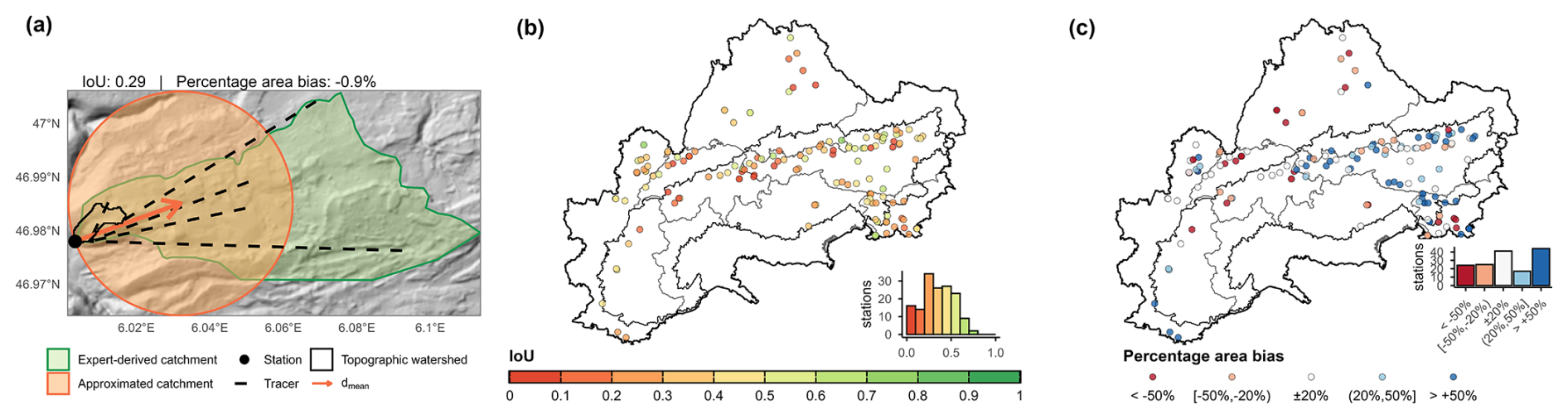
Figure A1Example and validation of catchment approximations. (a) Spatial overview for the Source du Verneau showing the topographic catchment, measuring station, positive tracer connections (DREAL Bourgogne Franche-Comté, 2020), expert-derived catchment (Charlier et al., 2014; Tissot and Tresse, 1978), shift direction , and the resulting catchment approximation. (b) Spatial distribution of Intersection over Union (IoU) between the approximations and known catchments for all sites. (c) Spatial overview of over- or underestimation of catchment area by the approximations relative to the known catchments. Administrative borders: © 2018–2025 GADM. Alpine Convention perimeter: (Eurac Research and Permanent Secretariat of the Alpine Convention, 2025).
The approach applied in the ALPAKAS dataset differs slightly from that described by Thinius et al. (2026), as tracer-test data were incorporated alongside topographic information whenever available. This additional information was considered because tracer tests are widely regarded as one of the most reliable methods for catchment delineation in karst regions (Goldscheider et al., 2008). Tracer tests were identified through literature review for 123 of the 243 stations in the dataset. For 77 of these stations, ALPAKAS also includes an expert-based catchment delineation. For the remaining 46 stations, positive tracer detections at the spring were reported, but no corresponding expert-based catchment delineation could be included in ALPAKAS. Given that tracer tests are commonly used to investigate and constrain catchment boundaries, this apparent discrepancy highlights that the expert-based catchment delineations available in ALPAKAS may not be exhaustive, as some delineations may not have been identified during the literature review or could not be included due to data-access or licensing restrictions.
For each of the N injection points with positive detection at the spring, the vector points from the station to the tracer injection location. The distance-weighted mean direction is then computed as
where and are unit vectors representing the topographic and tracer-derived directions, respectively. The corresponding weights are defined as
with denoting the distance from the spring to the nth injection point. Including the topographic watershed centroid as a pseudo-injection point ensures that both the topographic reference and the directions toward tracer injection points contribute proportionally, with longer distances receiving higher weighting. For the final catchment estimate, the circular buffer centered on the spring station is shifted along the normalized mean direction until the spring lies on the circle boundary, thereby representing the catchment outlet.
The approach was validated using the Intersection over Union (IoU) between the circular catchment approximation and the reference catchments, which was calculated for 151 measuring stations with known basins (Fig. A1b). An IoU of 1 means perfect agreement whereas 0 indicates no overlap at all. The median IoU is 0.34, reflecting the inability of a geometrically idealized circular approximation to reproduce the irregular shapes of natural catchments (e.g. the Source du Verneau; Fig. A1a). The incorporation of tracer-test data improved agreement with expert-based delineations in the dataset, increasing the median IoU from 0.30 to 0.34, particularly in regions where groundwater flow systems are only weakly controlled by surface topography. Since tracer data were available for approximately 51 % of stations in both the validation subset and the full dataset, this improvement in IoU observed in the validation subset may be considered broadly representative of the entire dataset. Area estimates derived from the simplified mass-balance approach exhibit a positive bias, particularly in the core Alpine region, and a negative bias in the European Foreland (Fig. A1c), with a median overestimation of 9 % across all stations. However, apparent over- or underestimation of recharge areas does not necessarily indicate true modelling errors, as the reference catchments themselves are subject to uncertainty and vary in both data quality and delineation methodology. Uncertainties associated with the method originate from ERA5-Land reanalysis input data and simplifying balance assumptions in step (i), as well as from the circular shape and the topography-based watershed delineation in step (ii). A detailed presentation and discussion of the catchment approximation method and its uncertainties can be found in Thinius et al. (2026).
Preprocessing steps were applied depending on the original temporal resolution class of the time series (Sect. 4.1) and are illustrated in the workflow presented in Fig. B1.
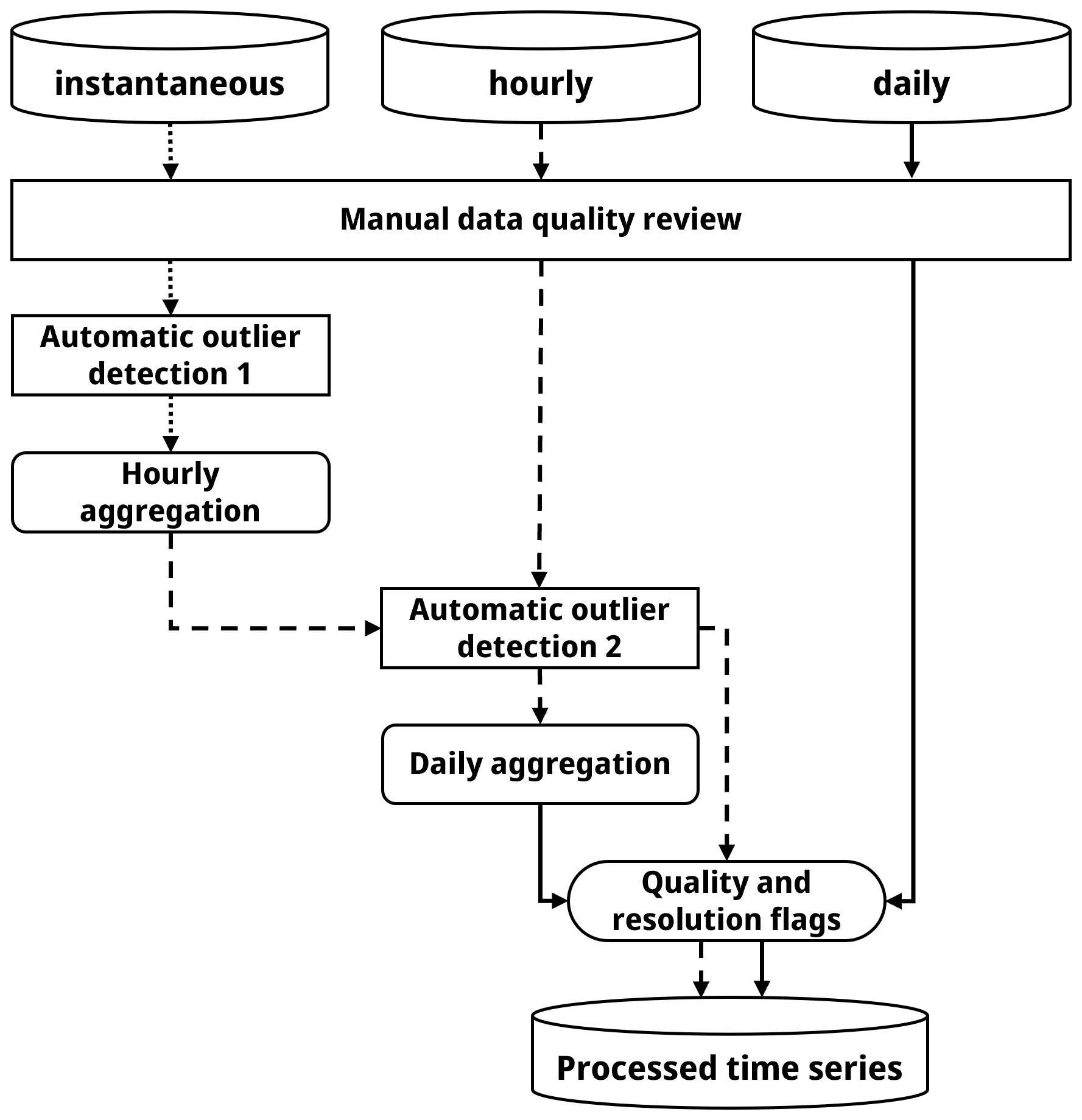
Figure B1Preprocessing workflow for discharge time series originally available at instantaneous, hourly, and daily temporal resolution classes.
B1 Manual data quality review
As an initial step of the preprocessing, a conservative manual screening of all discharge time series was performed to identify obvious outliers and artefacts based on expert judgement. Particular emphasis was placed on recession limbs, which were visually inspected and compared with similar recession events within the same time series to detect irregular behaviour. Identified artefacts primarily included plateaus caused by sensor cut-offs, abrupt step changes, extended segments indicative of linear interpolation, highly noisy periods, and other anomalous patterns. For stations with original data available at both hourly and daily resolution, dates in the daily time series corresponding to outliers or artefacts identified in the hourly data were also flagged.
B2 Automatic outlier detection
Subsequently, a novel automatic outlier detection approach was applied to specifically identify sharp dips and sharp spikes in the discharge time series, typically caused by sensor anomalies. The method is based on relative change rates within a percentile-based framework, whereby each observation is compared with mean change rates calculated separately for positive and negative changes within each decile of the time series. This allows the algorithm to account for variations in typical change rates depending on a data point's position within the hydrograph (e.g., along the recession limb). Sharp dips and sharp spikes are defined as sudden, localized reversals in the time series. Sharp dips correspond to pronounced decreases followed by abrupt increases, whereas sharp spikes represent pronounced increases followed by abrupt decreases. A sharp dip is flagged when the decrease relative to the preceding value falls below a negative threshold and the subsequent increase exceeds a corresponding positive threshold. Conversely, a sharp spike is identified when an initial increase exceeds the positive threshold and is followed by a decrease below the negative threshold. Thresholds are defined as a change rate factor multiplied by the mean positive or negative change rate within the respective decile. The respective conditions for sharp dips and sharp spikes were thus defined as
where rinc,i and rdec,i denote positive and negative relative change rates at observation i, respectively, and are the mean positive and negative change rates within the decile containing observation i, respectively, and Fdip and Fspike are the corresponding change rate factors. Change rate factors of Fdip = 10 and Fspike = 20 were empirically determined, with the more conservative factor for spikes chosen to avoid misclassifying genuine high-flow peaks as outliers. The reliability of the method was confirmed through ex post manual verification.
Automatic outlier detection was applied exclusively to hourly and instantaneous time series comprising at least 1000 observations after excluding segments with temporal resolutions lower than hourly. Multiple iterations were performed until the detection process converged, and no additional outliers were detected. The prior manual screening of outliers and artefacts was essential to prevent distortion of the data distribution. All identified outliers were flagged and retained in the dataset.
B3 Data aggregation
After removing identified outliers and artefacts, instantaneous time series were resampled to hourly values. Hourly values were calculated using time-weighted aggregation based on trapezoidal integration, equivalent to assuming linear change between consecutive observations, with each time interval contributing in proportion to its duration. A maximum gap length of one hour was allowed, ensuring that each hourly value contained at least one observed value. For hours with incomplete data coverage, integration was performed only over the available segments. Time stamps refer to the beginning of the aggregation interval.
For daily aggregation, missing hourly values were first linearly interpolated between consecutive observations separated by no more than 24 h. Daily values were then calculated as the arithmetic mean of all available observed and interpolated hourly values within each day. Under this interpolation criterion, each daily value contained at least one observed hourly value, while gaps of more than 23 consecutive missing hourly values were not interpolated. This procedure was also applied to time series containing one hourly observation per day recorded at a fixed time of day (e.g., at 04:00), rather than treating these observations directly as daily values. Because this recording time occasionally varied within individual time series, directly assigning these hourly observations as daily values could introduce temporal inconsistencies. Interpolation to an hourly time grid followed by aggregation over fixed calendar-day intervals ensured a consistent temporal reference between discharge and corresponding drivers such as meteorological inputs.
B4 Data quality and temporal resolution flags
To enable flexible and efficient data subsetting, additional flags describing data quality and temporal resolution were assigned to both the daily and hourly preprocessed time series. For each data point, the minimum temporal distance to the preceding or subsequent observation is provided and classified into temporal interval classes (hourly; ≤ daily; ≤ weekly; > weekly), thereby enabling the identification and removal of isolated observations. To facilitate the exclusion of periods with lower or heterogeneous measurement resolution, dominant temporal resolution classes were manually identified for extended periods and flagged accordingly (hourly; daily; subweekly; weekly; biweekly; monthly). Notably, changes in measurement frequency may reflect modifications in measurement methods or infrastructure. In addition, quality flags were manually assigned to periods characterized by reduced effective measurement resolution or increased noise. This quality assessment was based exclusively on internal characteristics and deviations within individual time series.
Finally, changepoint detection was applied to the daily (aggregated) time series using the Pruned Exact Linear Time (PELT) algorithm, as implemented in the changepoint package in R (Killick and Eckley, 2014). Changes in both the mean and variance of the time series were considered simultaneously by fitting segment-wise parametric models and identifying changepoints where the improvement in model fit exceeded the applied penalty. Prior to analysis, identified outliers and artefacts, as well as time series segments with a dominant temporal resolution coarser than daily were excluded. As PELT requires complete time series, short data gaps of up to four weeks were linearly interpolated, whereas longer gaps were excluded entirely to avoid detecting changepoints driven by interpolation-induced trends. The exclusion of extended gaps was not considered problematic, as the analysis aimed to identify sustained shifts in mean or variance rather than short-term fluctuations. To balance sensitivity and overfitting, the penalty parameter was manually calibrated following Killick and Eckley (2014) by multiplying a penalty factor with the logarithm of the number of daily values. After extensive testing, a penalty factor of 250 was found to provide the most robust results. This relatively high penalty was required to account for the potentially highly dynamic behaviour of karst systems and to restrict detection only on distinct changepoints. While the method effectively identified genuine changepoints across the time series, a small number of additional changepoints were detected during extended periods of low or absent discharge, as commonly observed for intermittent overflow springs. Manual post-validation was therefore performed to distinguish genuine structural changes from changepoints triggered by prolonged low-flow conditions. To enable flexible data selection, each observation was assigned a numerical segment flag, with an additional flag indicating the segment considered most reliable based on expert judgement. The final segmentation was subsequently transferred to the corresponding hourly time series to ensure consistency across temporal resolutions.
Water-quality observations are increasingly incorporated into large-sample hydrological datasets, as demonstrated by CAMELS-Chem (Sterle et al., 2024), CAMELS-CH-Chem (Do Nascimento et al., 2025), QUADICA v2 (Ebeling et al., 2026) and Caravan-Qual (Jones et al., 2026). Although water-quality observations are not included in ALPAKAS, complementary data are available from various monitoring networks. Water temperature and electrical conductivity are commonly monitored automatically alongside discharge at spring stations, providing continuous time series. Such records are available from several providers that supplied discharge data for ALPAKAS, including ARSO (2020), BAFU (2025a, b), BMLUK (2025), LfU (2025), Savoie (2025), and SNO KARST (2025a), while turbidity records are also available at selected stations.
The availability and temporal coverage of other water-quality parameters, including major ions, nutrients, organic carbon, trace elements, and pollutants such as pesticides, vary considerably among data providers and sites. These parameters are typically measured through periodic sampling, with more extensive monitoring often conducted at springs used for drinking-water supply due to additional water-quality requirements.
The SNO KARST dataset (Cinkus et al., 2026) combines spring discharge time series with physicochemical observations for 13 French karst springs, while the recently published ARETA dataset (Donnini et al., 2026) compiles physicochemical, chemical, and isotopic observations from more than 3000 Alpine spring-water analyses. However, the availability of these observations for individual ALPAKAS springs has not been systematically assessed. A future extension of ALPAKAS to include commonly monitored physicochemical time series, particularly water temperature and electrical conductivity, could be a first step towards improving our understanding of hydrological and hydrochemical processes in karst systems and supporting water-quality research on karst springs, which are often vulnerable to contamination.
Table D1Hydrometeorological time series available at daily and hourly resolution in ALPAKAS, including data quality and temporal resolution flags associated with the discharge hydrographs (Sect. 4.1).
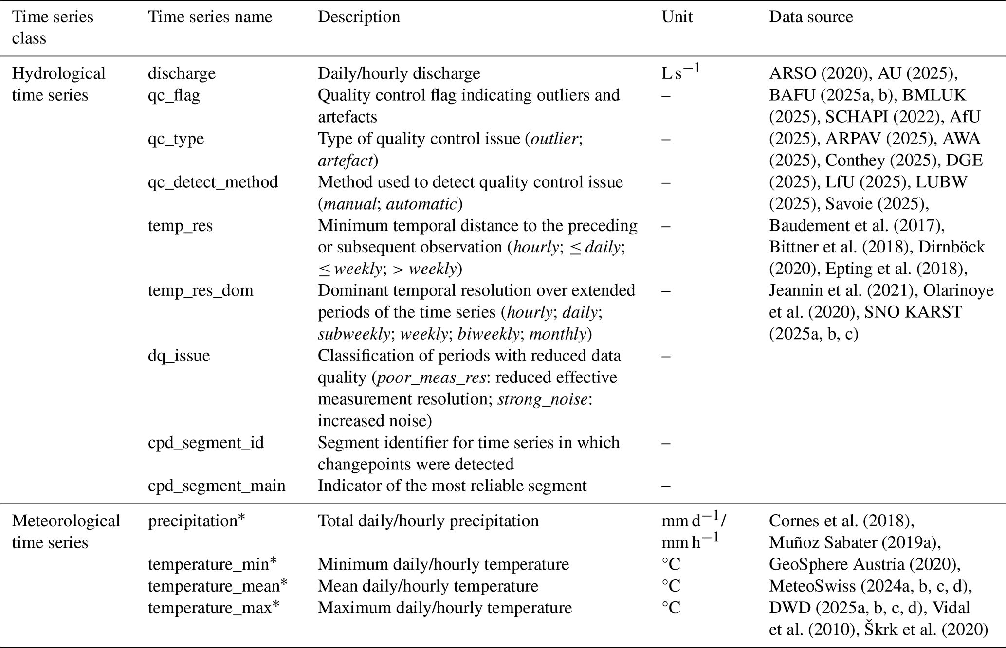
* Variables are provided separately for meteorological products: E-OBS (*_eobs), ERA5-Land (*_era5land) and national datasets (*_nat).
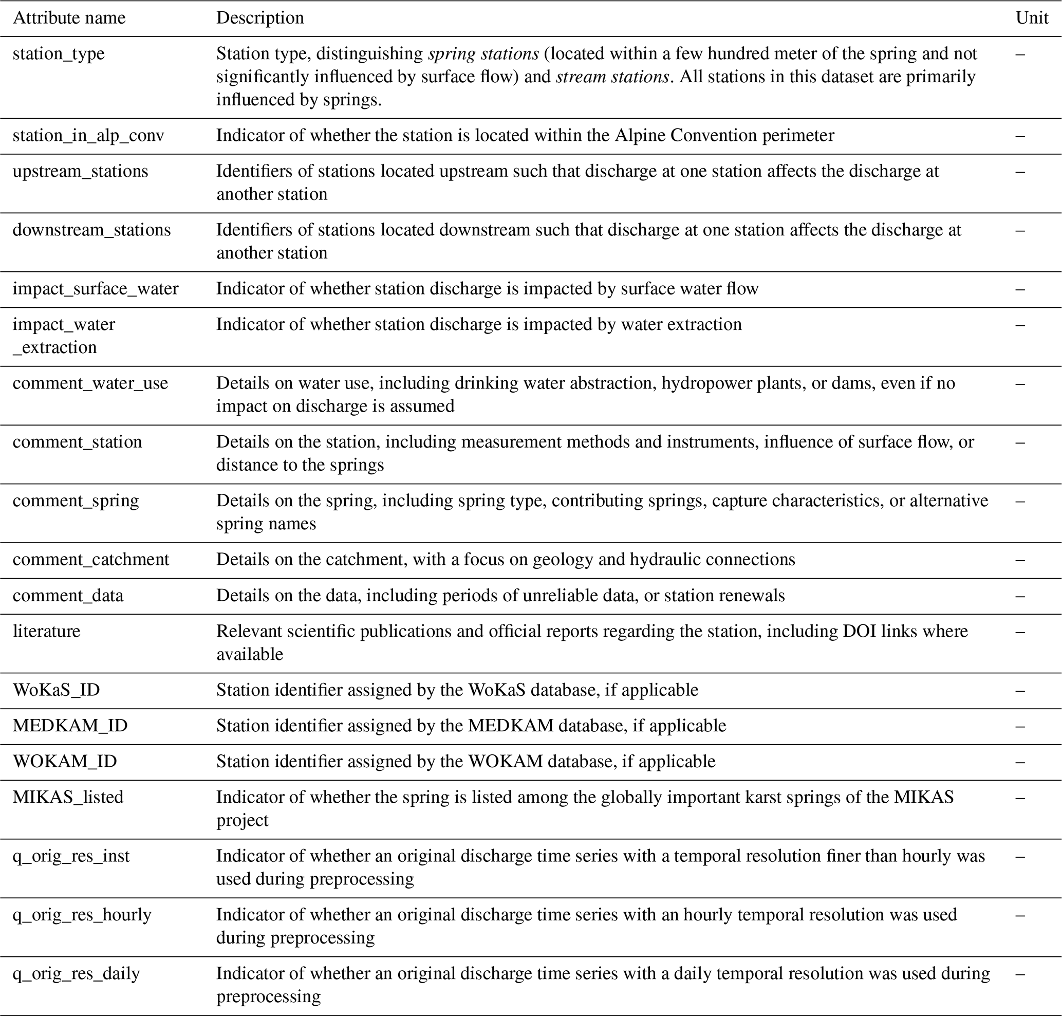
Table E2Static catchment attributes available in ALPAKAS related to topography and geographic positioning. [1–2] refer to Strahler stream orders 1 and 2, respectively.
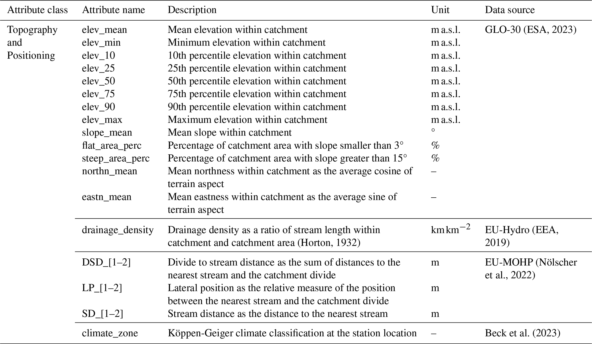
Table E3Static catchment attributes available in ALPAKAS related to meteorology and hydrology. Meteorological indicators are derived from daily time series of area-weighted catchment means, as described in Sect. 4.2.
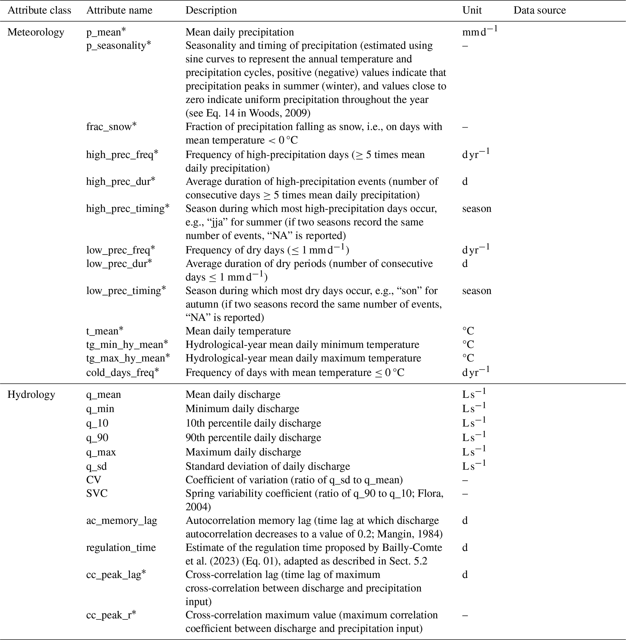
*Variables are provided separately for meteorological products: E-OBS (*_eobs), ERA5-Land (*_era5land) and national datasets (*_nat).
Table E4Static catchment attributes available in ALPAKAS related to land cover and glacier.
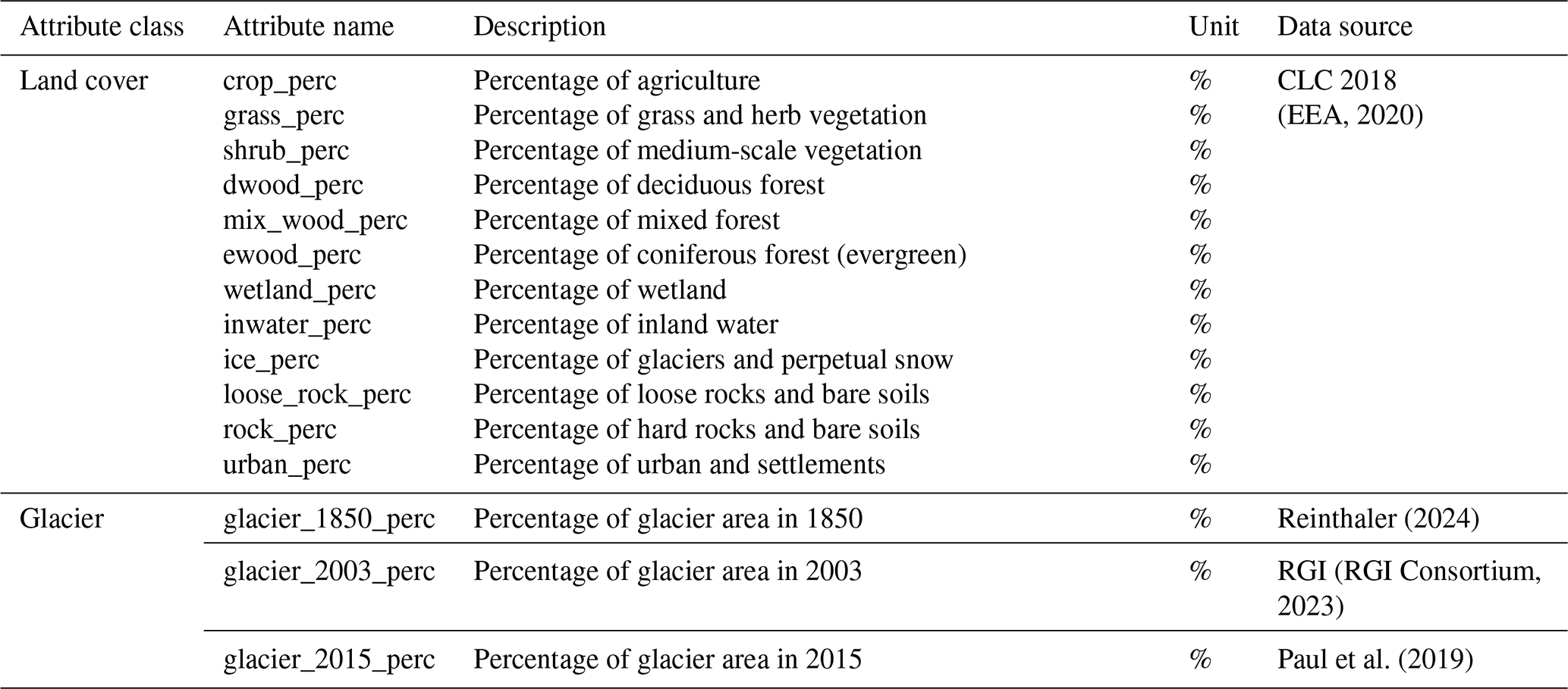
Table E5Static catchment attributes available in ALPAKAS related to soil.
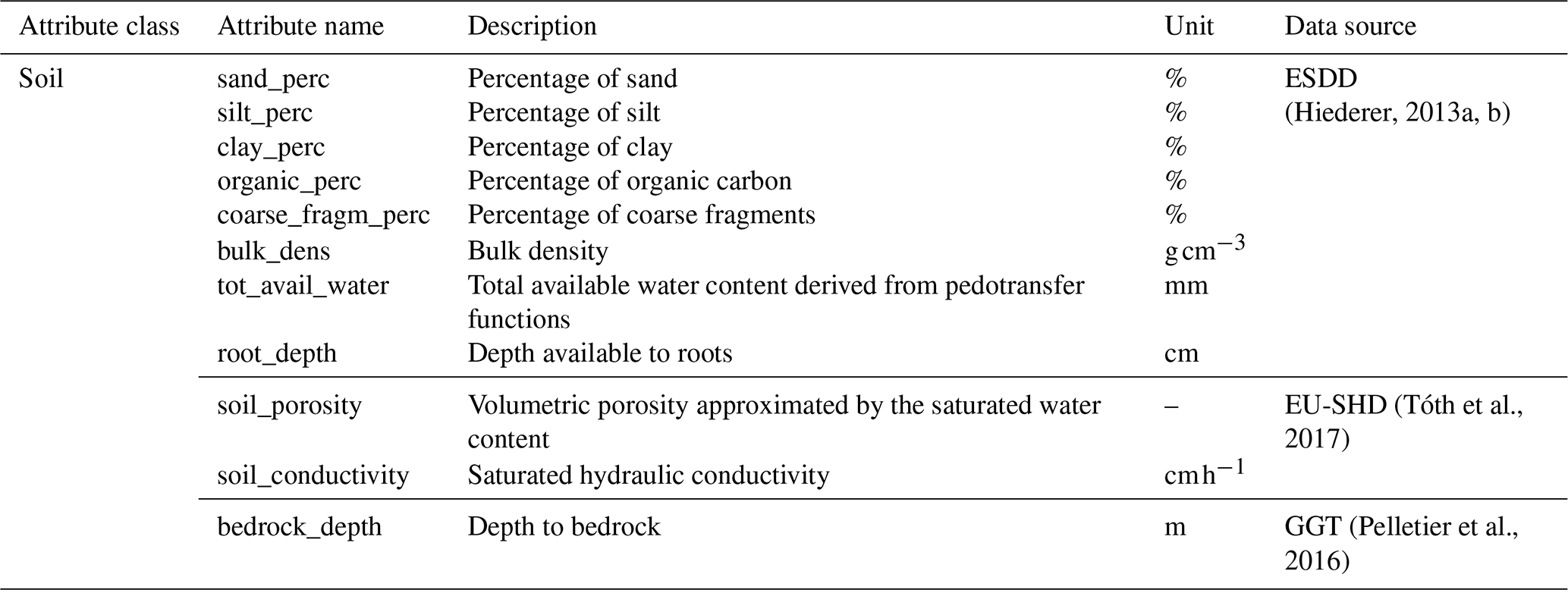
Table E6Static catchment attributes available in ALPAKAS related to hydrogeology. L1 and L4 indicate that the attribute is derived from the lithological levels 1 and 4 of the IHME1500 dataset, respectively.
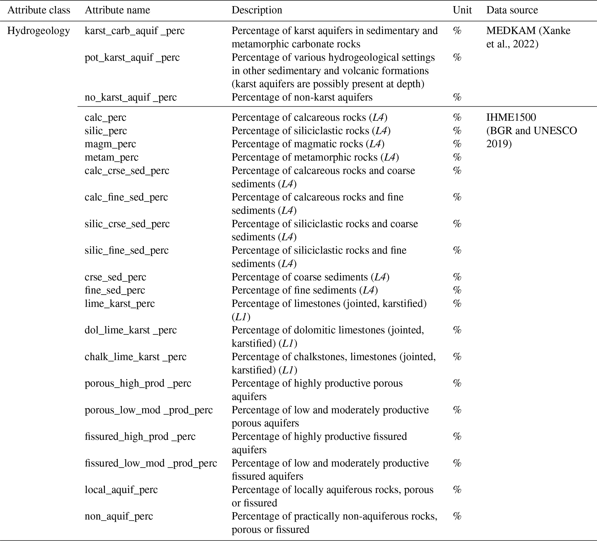
FJ requested the data with support from SB, PT, and NG. FJ performed the data preparation and processing under the supervision of SB and ZC and with support from PT. FJ wrote the manuscript, prepared the figures and tables, and maintained the code repository, with contributions from PT on the circular catchment approximations. All authors contributed to the methodological framework and to the review and editing of the manuscript.
The contact author has declared that none of the authors has any competing interests.
Publisher's note: Copernicus Publications remains neutral with regard to jurisdictional claims made in the text, published maps, institutional affiliations, or any other geographical representation in this paper. The authors bear the ultimate responsibility for providing appropriate place names. Views expressed in the text are those of the authors and do not necessarily reflect the views of the publisher.
The authors thank all data-providing institutions and individual researchers contributing to the ALPAKAS dataset. We extend our thanks to Nataša Ravbar for her expertise and support regarding Slovenian karst springs. We acknowledge the KARST observatory network initiated by INSU/CNRS for providing spring discharge data used in this study. We further thank Gerfried Winkler, Martin Masten, Magdalena Seelig and Simon Seelig for providing detailed catchments delineations for Austrian karst springs developed within the ECOSPRING project. Finally, we acknowledge the E-OBS dataset from the EU-FP6 project UERRA and the Copernicus Climate Change Service, and the data providers in the ECA&D project.
This work was funded by the German Research Foundation (DFG; grant number 529209885) and the Austrian Science Fund (FWF; grant number I 6688-N).
This paper was edited by Attila Demény and reviewed by Pierre-Yves Jeannin and Klaus Hinsby.
Addor, N., Newman, A. J., Mizukami, N., and Clark, M. P.: The CAMELS data set: catchment attributes and meteorology for large-sample studies, Hydrol. Earth Syst. Sci., 21, 5293–5313, https://doi.org/10.5194/hess-21-5293-2017, 2017. a, b, c, d
AfU (Amt für Umwelt): Canton of Solothurn, Switzerland, discharge data received: 25 March 2025, 2025. a, b
Amatulli, G., Domisch, S., Tuanmu, M.-N., Parmentier, B., Ranipeta, A., Malczyk, J., and Jetz, W.: A suite of global, cross-scale topographic variables for environmental and biodiversity modeling, Sci. Data, 5, 180040, https://doi.org/10.1038/sdata.2018.40, 2018. a
ARPAV (Agenzia Regionale per la Prevenzione e Protezione Ambiental del Veneto): Italy, discharge data received: 12 August 2025, 2025. a, b
ARSO: Arhivski hidrološki podatki, Agencija Republike Slovenije za okolje (ARSO) [data set], https://www.arso.gov.si/vode/podatki/ (last access: 27 March 2025), 2020. a, b, c
AU (Amt für Umwelt): Fürstentum Liechtenstein, discharge data received: 10 June 2025, 2025. a, b
AWA (Amt für Wasser und Abfall): Canton of Bern, Switzerland, discharge data received: 2 April 2025, 2025. a, b
BAFU: Nationale Grundwasserbeobachtung NAQUA, Bundesamt für Umwelt (BAFU) – Abteilung Hydrologie, discharge data received: 28 January 2025, 2025a. a, b, c
BAFU: Basismessnetz Oberflächengewässer, Bundesamt für Umwelt (BAFU) – Abteilung Hydrologie, discharge data received: 30 January 2025, 2025b. a, b, c
Bailly-Comte, V., Ladouche, B., Charlier, J. B., Hakoun, V., and Maréchal, J. C.: XLKarst, an Excel tool for time series analysis, spring recession curve analysis and classification of karst aquifers, Hydrogeol. J., 31, 2401–2415, https://doi.org/10.1007/s10040-023-02710-w, 2023. a, b
Barthel, R., Haaf, E., Nygren, M., and Giese, M.: Systematic visual analysis of groundwater hydrographs: potential benefits and challenges, Hydrogeol. J., 30, 359–378, https://doi.org/10.1007/s10040-021-02433-w, 2022. a
Baston, D.: exactextractr: Fast Extraction from Raster Datasets using Polygons, version 0.10.1, CRAN [code], https://doi.org/10.32614/CRAN.package.exactextractr, 2025. a
Baudement, C., Arfib, B., Mazzilli, N., Jouves, J., Lamarque, T., and Guglielmi, Y.: Groundwater management of a highly dynamic karst by assessing baseflow and quickflow with a rainfall-discharge model (Dardennes springs, SE France), B. Soc. Géol. Fr., 188, 40, https://doi.org/10.1051/bsgf/2017203, 2017. a, b
Beck, H. E., McVicar, T. R., Vergopolan, N., Berg, A., Lutsko, N. J., Dufour, A., Zeng, Z., Jiang, X., Van Dijk, A. I. J. M., and Miralles, D. G.: High-resolution (1 km) Köppen-Geiger maps for 1901–2099 based on constrained CMIP6 projections, Sci. Data, 10, 724, https://doi.org/10.1038/s41597-023-02549-6, 2023. a, b
Beniston, M., Farinotti, D., Stoffel, M., Andreassen, L. M., Coppola, E., Eckert, N., Fantini, A., Giacona, F., Hauck, C., Huss, M., Huwald, H., Lehning, M., López-Moreno, J.-I., Magnusson, J., Marty, C., Morán-Tejéda, E., Morin, S., Naaim, M., Provenzale, A., Rabatel, A., Six, D., Stötter, J., Strasser, U., Terzago, S., and Vincent, C.: The European mountain cryosphere: a review of its current state, trends, and future challenges, The Cryosphere, 12, 759–794, https://doi.org/10.5194/tc-12-759-2018, 2018. a
BGR and UNESCO: International Hydrogeological Map of Europe 1 : 1,500,000 – version 1.2, Bundesanstalt für Geowissenschaften und Rohstoffe (BGR) and UNESCO [data set], https://metadata.europe-geology.eu/record/basic/341255A9-180F-4BF9-B96F-D085339EA86D (last access: 16 November 2026), 2019. a, b, c
Bittner, D., Narany, T. S., Kohl, B., Disse, M., and Chiogna, G.: Modeling the hydrological impact of land use change in a dolomite-dominated karst system, J. Hydrol., 567, 267–279, https://doi.org/10.1016/j.jhydrol.2018.10.017, 2018. a, b
BMLUK (Bundesministerium für Land- und Forstwirtschaft, Klima- und Umweltschutz, Regionen und Wasserwirtschaft) – Abteilung Wasserhaushalt: discharge data received: December 2025, 2025. a, b, c
Bongiovanni, G., Matiu, M., Crespi, A., Napoli, A., Majone, B., and Zardi, D.: EEAR-Clim: a high-density observational dataset of daily precipitation and air temperature for the Extended European Alpine Region, Earth Syst. Sci. Data, 17, 1367–1391, https://doi.org/10.5194/essd-17-1367-2025, 2025. a, b, c
Çallı, S. S., Özdemir Çallı, K., Akdim, B., Arfib, B., Benderev, A., Beranger, S., Burg, A., Can, O., Charlier, J.-B., Çelik, M., Çetin, A. M., Chemseddine, F., Deliyska, M., Di Matteo, L., Dionigi, M., Eftimi, R., Eybl, J., Fronzi, D., Goldscheider, N., Gökkaya, E., Jodar, J., Jourde, H., Kaminsky, E., Katsanou, K., Kavousi, A., Kaya, M., Labat, D., Liesch, T., Malik, P., Massari, C., Mayaud, C., Mazzilli, N., Pracny, P., Ravbar, N., Rispal, N., Seelig, S., Sivelle, V., Steinmann, M., Valigi, D., Winkler, G., Yahşi, A. K., and Hartmann, A.: High-Resolution Karst Spring Discharge Datasets of the Euro-Mediterranean Mountain Regions, Earth Syst. Sci. Data Discuss. [preprint], https://doi.org/10.5194/essd-2026-281, in review, 2026. a
Charlier, J.-B., Desprats, J.-F., and Ladouche, B.: Appui au SCHAPI 2014 – Module 1: Rôle et contribution des eaux souterraines d'origine karstique dans les crues de la Loue à Chenecey-Buillon, Tech. Rep. BRGM/RP-63844-FR, BRGM, https://orisk-bfc.fr/telechargement/fichier/5173 (last access: 16 November 2026), 2014. a
Chen, Z., Auler, A. S., Bakalowicz, M., Drew, D., Griger, F., Hartmann, J., Jiang, G., Moosdorf, N., Richts, A., Stevanovic, Z., Veni, G., and Goldscheider, N.: The World Karst Aquifer Mapping project: concept, mapping procedure and map of Europe, Hydrogeol. J., 25, 771–785, https://doi.org/10.1007/s10040-016-1519-3, 2017. a, b
Chen, Z., Hartmann, A., Wagener, T., and Goldscheider, N.: Dynamics of water fluxes and storages in an Alpine karst catchment under current and potential future climate conditions, Hydrol. Earth Syst. Sci., 22, 3807–3823, https://doi.org/10.5194/hess-22-3807-2018, 2018. a
Cinkus, G., Mazzilli, N., and Jourde, H.: KarstID: an R Shiny application for the analysis of karst spring discharge time series and the classification of karst system hydrological functioning, Environ. Earth Sci., 82, 136, https://doi.org/10.1007/s12665-023-10830-5, 2023. a, b
Cinkus, G., Bondu, R., Aliouache, M., Jourde, H., Mazzilli, N., Arfib, B., Bailly-Comte, V., Batiot-Guilhe, C., Celle, H., Delbart, C., Fournier, M., Labat, D., Peyraube, N., Steinmann, M., Valdès-Lao, D., Baudement, C., Béranger, S., Binet, S., Boetsch, A., Brunet, P., Carrière, S. D., Chalikakis, K., Charlier, J.-B., Cousquer, Y., Défarge, C., Ducasse, J., Emblanch, C., Fabre, J., Fleury, P., Garin, T., Huon, J., Jardani, A., Johannet, A., Jouves, J., Jozja, N., Justy, L., Ladouche, B., Lamarque, T., Lastennet, R., Léonardi, V., Lobry, O., Lorette, G., Loup, C., Marchand, P., Manière, L., Maréchal, J.-C., Martin, L., Muller, R., Massei, N., Naessens, F., Ollivier, C., Probst, A., Seidel, J.-L., Serene, L., Sivelle, V., and Zappelli, A.: Comprehensive dataset of continuously monitored hydrodynamic and physico-chemical parameters in various karst systems, France, Sci. Data, https://doi.org/10.1038/s41597-026-07561-0, 2026. a
Clerc-Schwarzenbach, F., Selleri, G., Neri, M., Toth, E., van Meerveld, I., and Seibert, J.: Large-sample hydrology – a few camels or a whole caravan?, Hydrol. Earth Syst. Sci., 28, 4219–4237, https://doi.org/10.5194/hess-28-4219-2024, 2024. a
Conthey: Commune de Conthey, Canton of Valais, Switzerland, discharge data received: 27 January 2025, 2025. a, b
Cornes, R. C., Van Der Schrier, G., Van Den Besselaar, E. J. M., and Jones, P. D.: An Ensemble Version of the E-OBS Temperature and Precipitation Data Sets, J. Geophys. Res.-Atmos., 123, 9391–9409, https://doi.org/10.1029/2017JD028200, 2018. a, b, c, d
Coxon, G., Addor, N., Bloomfield, J. P., Freer, J., Fry, M., Hannaford, J., Howden, N. J. K., Lane, R., Lewis, M., Robinson, E. L., Wagener, T., and Woods, R.: CAMELS-GB: hydrometeorological time series and landscape attributes for 671 catchments in Great Britain, Earth Syst. Sci. Data, 12, 2459–2483, https://doi.org/10.5194/essd-12-2459-2020, 2020. a
Delaigue, O., Guimarães, G. M., Brigode, P., Génot, B., Perrin, C., Soubeyroux, J.-M., Janet, B., Addor, N., and Andréassian, V.: CAMELS-FR dataset: a large-sample hydroclimatic dataset for France to explore hydrological diversity and support model benchmarking, Earth Syst. Sci. Data, 17, 1461–1479, https://doi.org/10.5194/essd-17-1461-2025, 2025. a
DGE: Veille Hydro-météorologique du Canton de Vaud, Direction générale de l'environnement (DGE), Canton of Vaud, Switzerland, https://www.vhv.ch/xt_vh_718536/index.php?ck3_page_reloaded=1 (last access: 3 December 2025), 2025. a, b
Dirnböck, T.: LTER Zöbelboden, Austria, Runoff Catchment 2000–2019 – version 3, EUDAT B2SHARE [data set], https://doi.org/10.23728/B2SHARE.7F0E7167653449BC809739C7027B354A, 2020. a, b
Do Nascimento, T. V. M., Höge, M., Schönenberger, U., Pool, S., Siber, R., Kauzlaric, M., Staudinger, M., Horton, P., Floriancic, M. G., Storck, F. R., Rinta, P., Seibert, J., and Fenicia, F.: Swiss data quality: augmenting CAMELS-CH with isotopes, water quality, agricultural and atmospheric data, Sci. Data, 12, 1283, https://doi.org/10.1038/s41597-025-05625-1, 2025. a
Donnini, M., Melelli, L., Vetuschi Zuccolini, M., Fiorucci, F., Cardellini, C., and Frondini, F.: ARETA (Alpine caRbon cyclE daTAset): a dataset on physical, chemical and isotopic data of Alpine groundwaters, Sci. Data, 13, 734, https://doi.org/10.1038/s41597-025-06541-0, 2026. a
DREAL Bourgogne Franche-Comté: Traçages des eaux souterraines en Bourgogne-Franche-Comté: circulation identifiée, https://www.data.gouv.fr/datasets/tracages-des-eaux-souterraines-en-bourgogne-franche-comte-circulation-identifiee (last access: 2 January 2026), 2020. a
DWD: Raster data set of daily precipitation sums in mm for Germany – HYRAS-DE-PR, Version v6.0, Deutscher Wetterdienst (DWD) [data set], https://opendata.dwd.de/climate_environment/CDC/grids_germany/daily/hyras_de/precipitation/ (last access: 11 July 2025), 2025a. a, b, c
DWD: Raster data set of daily mean temperature in °C for Germany – HYRAS-DE-TAS, Version v6.0, Deutscher Wetterdienst (DWD) [data set], https://opendata.dwd.de/climate_environment/CDC/grids_germany/daily/hyras_de/air_temperature_mean/ (last access: 11 July 2025), 2025b. a, b, c
DWD: Raster data set of daily maximum temperature in °C for Germany – HYRAS-DE-TASMAX, Version v6.0, Deutscher Wetterdienst (DWD) [data set], https://opendata.dwd.de/climate_environment/CDC/grids_germany/daily/hyras_de/air_temperature_max/ (last access: 11 July 2025), 2025c. a, b, c
DWD: Raster data set of daily minimum temperature in °C for Germany – HYRAS-DE-TASMIN, Version v6.0, Deutscher Wetterdienst (DWD) [data set], https://opendata.dwd.de/climate_environment/CDC/grids_germany/daily/hyras_de/air_temperature_min/ (last access: 11 July 2025), 2025d. a, b, c
Ebeling, P., Hubig, A., Wachholz, A., Scharfenberger, U., Haug, S., Nguyen, T., Sarrazin, F., Batool, M., Musolff, A., and Kumar, R.: QUADICA v2: extending the large-sample data set for water QUAlity, DIscharge and Catchment Attributes in Germany, Earth Syst. Sci. Data, 18, 691–712, https://doi.org/10.5194/essd-18-691-2026, 2026. a
EEA: EU-Hydro River Network Database 2006–2012 (vector), Europe – version 1.3, Nov. 2020, European Environment Agency (EEA) [data set], https://doi.org/10.2909/393359A7-7EBD-4A52-80AC-1A18D5F3DB9C, 2019. a, b
EEA: CORINE Land Cover 2018 (vector) – version 2020_20u1, European Environment Agency (EEA) [data set], https://doi.org/10.2909/71C95A07-E296-44FC-B22B-415F42ACFDF0, 2020. a, b
Epting, J., Page, R. M., Auckenthaler, A., and Huggenberger, P.: Process-based monitoring and modeling of Karst springs – Linking intrinsic to specific vulnerability, Sci. Total Environ., 625, 403–415, https://doi.org/10.1016/j.scitotenv.2017.12.272, 2018. a, b
ESA: Copernicus GLO-30 DEM – version 2023_1, European Space Agency (ESA) [data set], https://doi.org/10.5270/ESA-c5d3d65, 2023. a, b, c, d
Eurac Research and Permanent Secretariat of the Alpine Convention: Alpine Convention perimeter, Permanent Secretariat of the Alpine Convention [data set], https://doi.org/10.48784/VK93-8P54, 2025. a, b, c, d
Flora, S. P.: Hydrogeological characterization and discharge variability of springs in the Middle Verde River watershed, Central Arizona, Master's thesis, Northern Arizona University, https://in.nau.edu/wp-content/uploads/sites/55/2018/09/Flora_Thesis_2004-ek.pdf (last access: 16 November 2026), 2004. a, b
Ford, D. and Williams, P.: Analysis of Karst Drainage Systems, in: Karst Hydrogeology and Geomorphology, 145–208, John Wiley & Sons, Ltd, ISBN 978-1-118-68498-6, https://doi.org/10.1002/9781118684986.ch6, 2007. a
GeoSphere Austria: SPARTACUS v2.1 Tagesdaten, GeoSphere Austria [data set], https://doi.org/10.60669/M6W8-S545, 2020. a, b, c
Goldscheider, N. and Drew, D. (Eds.): Methods in karst hydrogeology, vol. 26 of International contributions to hydrogeology, Taylor and Francis, ISBN 978-0-415-42873-6, https://doi.org/10.1201/9781482266023, 2007. a
Goldscheider, N., Meiman, J., Pronk, M., and Smart, C.: Tracer tests in karst hydrogeology and speleology, Int. J. Speleol., 37, 27–40, https://doi.org/10.5038/1827-806X.37.1.3, 2008. a
Goldscheider, N., Chen, Z., Auler, A. S., Bakalowicz, M., Broda, S., Drew, D., Hartmann, J., Jiang, G., Moosdorf, N., Stevanovic, Z., and Veni, G.: Global distribution of carbonate rocks and karst water resources, Hydrogeol. J., 28, 1661–1677, https://doi.org/10.1007/s10040-020-02139-5, 2020. a
Goldscheider, N., Xanke, J., and Liesch, T.: Verbreitung von Carbonatgesteinen und Karstwasserressourcen im Alpenraum, Grundwasser, 30, 211–226, https://doi.org/10.1007/s00767-025-00596-x, 2025. a, b
Hengl, T., Mendes De Jesus, J., Heuvelink, G. B. M., Ruiperez Gonzalez, M., Kilibarda, M., Blagotić, A., Shangguan, W., Wright, M. N., Geng, X., Bauer-Marschallinger, B., Guevara, M. A., Vargas, R., MacMillan, R. A., Batjes, N. H., Leenaars, J. G. B., Ribeiro, E., Wheeler, I., Mantel, S., and Kempen, B.: SoilGrids250m: Global gridded soil information based on machine learning, PLOS ONE, 12, e0169748, https://doi.org/10.1371/journal.pone.0169748, 2017. a
Hiederer, R.: Mapping soil properties for Europe: spatial representation of soil database attributes, no. EUR26082EN in Scientific and Technical Research Series, Publications Office of the European Union, Luxembourg, ISBN 978-92-79-32516-8, https://doi.org/10.2788/94128, 2013a. a, b
Hiederer, R.: Mapping soil typologies: spatial decision support applied to the European Soil Database, no. EUR25932EN in Scientific and Technical Research Series, Publications Office of the European Union, Luxembourg, https://doi.org/10.2788/87286, 2013b. a, b
Höge, M., Kauzlaric, M., Siber, R., Schönenberger, U., Horton, P., Schwanbeck, J., Floriancic, M. G., Viviroli, D., Wilhelm, S., Sikorska-Senoner, A. E., Addor, N., Brunner, M., Pool, S., Zappa, M., and Fenicia, F.: CAMELS-CH: hydro-meteorological time series and landscape attributes for 331 catchments in hydrologic Switzerland, Earth Syst. Sci. Data, 15, 5755–5784, https://doi.org/10.5194/essd-15-5755-2023, 2023. a, b, c
Horton, R. E.: Drainage‐basin characteristics, EOS T. Am. Geophys. Un., 13, 350–361, https://doi.org/10.1029/TR013i001p00350, 1932. a, b
Jeannin, P.-Y., Artigue, G., Butscher, C., Chang, Y., Charlier, J.-B., Duran, L., Gill, L., Hartmann, A., Johannet, A., Jourde, H., Kavousi, A., Liesch, T., Liu, Y., Lüthi, M., Malard, A., Mazzilli, N., Pardo-Igúzquiza, E., Thiéry, D., Reimann, T., Schuler, P., Wöhling, T., and Wunsch, A.: Karst modelling challenge 1: Results of hydrological modelling, J. Hydrol., 600, 126508, https://doi.org/10.1016/j.jhydrol.2021.126508, 2021. a, b
Jeannin, P.-Y., Malard, A., and Sinreich, M.: Advanced Approach to Assess Groundwater Storage and Water Availability in Karst Aquifers at Regional Scale, Hydrology, 13, 226, https://doi.org/10.3390/hydrology13090226, 2026. a, b, c
Joger, F. and Thinius, P.: FelixJoger/ALPAKAS: ALPAKAS Code Release v1.0, Zenodo [code], https://doi.org/10.5281/zenodo.24159191, 2026. a
Joger, F., Thinius, P., Chen, Z., Hartmann, A., Goldscheider, N., Liesch, T., Schubert, G., and Broda, S.: ALPAKAS: ALPine hydrographs and catchment Attributes for KArst Springs, Zenodo [data set], https://doi.org/10.5281/zenodo.23592639, 2026. a, b
Jones, E. R., Kratzert, F., and Van Vliet, M. T. H.: Caravan-Qual: A global scale integration of stream water quality observations into a large-sample hydrology dataset, Sci. Data, 13, 1015, https://doi.org/10.1038/s41597-026-07352-7, 2026. a
Killick, R. and Eckley, I. A.: changepoint: An R Package for Changepoint Analysis, J. Stat. Softw., 58, 1–27, https://doi.org/10.18637/jss.v058.i03, 2014. a, b
Klingler, C., Schulz, K., and Herrnegger, M.: LamaH-CE: LArge-SaMple DAta for Hydrology and Environmental Sciences for Central Europe, Earth Syst. Sci. Data, 13, 4529–4565, https://doi.org/10.5194/essd-13-4529-2021, 2021. a
Kotlarski, S., Gobiet, A., Morin, S., Olefs, M., Rajczak, J., and Samacoïts, R.: 21st Century alpine climate change, Clim. Dynam., 60, 65–86, https://doi.org/10.1007/s00382-022-06303-3, 2023. a
Kratzert, F., Klotz, D., Shalev, G., Klambauer, G., Hochreiter, S., and Nearing, G.: Towards learning universal, regional, and local hydrological behaviors via machine learning applied to large-sample datasets, Hydrol. Earth Syst. Sci., 23, 5089–5110, https://doi.org/10.5194/hess-23-5089-2019, 2019. a
Kratzert, F., Nearing, G., Addor, N., Erickson, T., Gauch, M., Gilon, O., Gudmundsson, L., Hassidim, A., Klotz, D., Nevo, S., Shalev, G., and Matias, Y.: Caravan – A global community dataset for large-sample hydrology, Sci. Data, 10, 61, https://doi.org/10.1038/s41597-023-01975-w, 2023. a
LfU (Bayerisches Landesamt für Umwelt): Gewässerkundlicher Dienst, discharge data received: 27 March 2025, 2025. a, b, c
Lindsay, J. B.: Whitebox GAT: A case study in geomorphometric analysis, Comput. Geosci., 95, 75–84, https://doi.org/10.1016/j.cageo.2016.07.003, 2016. a
Linsbauer, A., Huss, M., Hodel, E., Bauder, A., Fischer, M., Weidmann, Y., Bärtschi, H., and Schmassmann, E.: The New Swiss Glacier Inventory SGI2016: From a Topographical to a Glaciological Dataset, Front. Earth Sci., 9, 704189, https://doi.org/10.3389/feart.2021.704189, 2021. a
Loritz, R., Dolich, A., Acuña Espinoza, E., Ebeling, P., Guse, B., Götte, J., Hassler, S. K., Hauffe, C., Heidbüchel, I., Kiesel, J., Mälicke, M., Müller-Thomy, H., Stölzle, M., and Tarasova, L.: CAMELS-DE: hydro-meteorological time series and attributes for 1582 catchments in Germany, Earth Syst. Sci. Data, 16, 5625–5642, https://doi.org/10.5194/essd-16-5625-2024, 2024. a
LUBW (Landesanstalt für Umwelt Baden-Württemberg): Gewässerkundlicher Dienst, discharge data received: 16 June 2025, 2025. a, b
Mangin, A.: Pour une meilleure connaissance des systèmes hydrologiques à partir des analyses corrélatoire et spectrale, J. Hydrol., 67, 25–43, https://doi.org/10.1016/0022-1694(84)90230-0, 1984. a, b
MeteoSwiss: RhiresD: Daily precipitation (final analysis), Federal Office of Meteorology and Climatology [data set], https://opendatadocs.meteoswiss.ch/c-climate-data/c3-ground-based-climate-data (last access: 5 November 2025), 2024a. a, b, c
MeteoSwiss: TabsD: Daily mean temperature, Federal Office of Meteorology and Climatology [data set], https://opendatadocs.meteoswiss.ch/c-climate-data/c3-ground-based-climate-data (last access: 5 November 2025), 2024b. a, b, c
MeteoSwiss: TmaxD: Daily maximum temperature, Federal Office of Meteorology and Climatology [data set], https://opendatadocs.meteoswiss.ch/c-climate-data/c3-ground-based-climate-data (last access: 5 November 2025), 2024c. a, b, c
MeteoSwiss: TminD: Daily minimum temperature, Federal Office of Meteorology and Climatology [data set], https://opendatadocs.meteoswiss.ch/c-climate-data/c3-ground-based-climate-data (last access: 5 November 2025), 2024d. a, b, c
Moraga, J. S., Peleg, N., Fatichi, S., Molnar, P., and Burlando, P.: Revealing the impacts of climate change on mountainous catchments through high-resolution modelling, J. Hydrol., 603, 126806, https://doi.org/10.1016/j.jhydrol.2021.126806, 2021. a
Muñoz Sabater, J.: ERA5-Land hourly data from 1950 to present, Copernicus Climate Change Service (C3S) Climate Data Store (CDS) [data set], https://doi.org/10.24381/CDS.E2161BAC, 2019a. a, b, c
Muñoz Sabater, J.: ERA5-Land monthly averaged data from 1950 to present, Copernicus Climate Change Service (C3S) Climate Data Store (CDS) [data set], https://doi.org/10.24381/cds.68d2bb30, 2019b. a
Nearing, G., Cohen, D., Dube, V., Gauch, M., Gilon, O., Harrigan, S., Hassidim, A., Klotz, D., Kratzert, F., Metzger, A., Nevo, S., Pappenberger, F., Prudhomme, C., Shalev, G., Shenzis, S., Tekalign, T. Y., Weitzner, D., and Matias, Y.: Global prediction of extreme floods in ungauged watersheds, Nature, 627, 559–563, https://doi.org/10.1038/s41586-024-07145-1, 2024. a
Newman, A. J., Clark, M. P., Sampson, K., Wood, A., Hay, L. E., Bock, A., Viger, R. J., Blodgett, D., Brekke, L., Arnold, J. R., Hopson, T., and Duan, Q.: Development of a large-sample watershed-scale hydrometeorological data set for the contiguous USA: data set characteristics and assessment of regional variability in hydrologic model performance, Hydrol. Earth Syst. Sci., 19, 209–223, https://doi.org/10.5194/hess-19-209-2015, 2015. a
Nölscher, M., Mutz, M., and Broda, S.: EU-MOHP v013.1.1 Dataset, HydroShare [data set], https://doi.org/10.4211/HS.0D6999591FB048CAB5AB71FCB690EADB, 2022. a, b
Ohmer, M., Liesch, T., Habbel, B., Heudorfer, B., Gomez, M., Clos, P., Nölscher, M., and Broda, S.: GEMS-GER: a machine learning benchmark dataset of long-term groundwater levels in Germany with meteorological forcings and site-specific environmental features, Earth Syst. Sci. Data, 18, 77–95, https://doi.org/10.5194/essd-18-77-2026, 2026. a
Olarinoye, T., Gleeson, T., Marx, V., Seeger, S., Adinehvand, R., Allocca, V., Andreo, B., Apaéstegui, J., Apolit, C., Arfib, B., Auler, A., Bailly-Comte, V., Barberá, J. A., Batiot-Guilhe, C., Bechtel, T., Binet, S., Bittner, D., Blatnik, M., Bolger, T., Brunet, P., Charlier, J.-B., Chen, Z., Chiogna, G., Coxon, G., De Vita, P., Doummar, J., Epting, J., Fleury, P., Fournier, M., Goldscheider, N., Gunn, J., Guo, F., Guyot, J. L., Howden, N., Huggenberger, P., Hunt, B., Jeannin, P.-Y., Jiang, G., Jones, G., Jourde, H., Karmann, I., Koit, O., Kordilla, J., Labat, D., Ladouche, B., Liso, I. S., Liu, Z., Maréchal, J.-C., Massei, N., Mazzilli, N., Mudarra, M., Parise, M., Pu, J., Ravbar, N., Sanchez, L. H., Santo, A., Sauter, M., Seidel, J.-L., Sivelle, V., Skoglund, R. Ø., Stevanovic, Z., Wood, C., Worthington, S., and Hartmann, A.: Global karst springs hydrograph dataset for research and management of the world's fastest-flowing groundwater, Sci. Data, 7, 59, https://doi.org/10.1038/s41597-019-0346-5, 2020. a, b, c
Paul, F., Frey, H., and Le Bris, R.: A new glacier inventory for the European Alps from Landsat TM scenes of 2003: challenges and results, Ann. Glaciol., 52, 144–152, https://doi.org/10.3189/172756411799096295, 2011. a
Paul, F., Rastner, P., Azzoni, R. S., Diolaiuti, G., Fugazza, D., Le Bris, R., Nemec, J., Rabatel, A., Ramusovic, M., Schwaizer, G., and Smiraglia, C.: Glacier inventory of the Alps from Sentinel-2, shape files, PANGAEA [data set], https://doi.org/10.1594/PANGAEA.909133, 2019. a, b
Paul, F., Rastner, P., Azzoni, R. S., Diolaiuti, G., Fugazza, D., Le Bris, R., Nemec, J., Rabatel, A., Ramusovic, M., Schwaizer, G., and Smiraglia, C.: Glacier shrinkage in the Alps continues unabated as revealed by a new glacier inventory from Sentinel-2, Earth Syst. Sci. Data, 12, 1805–1821, https://doi.org/10.5194/essd-12-1805-2020, 2020. a
Pelletier, J., Broxton, P., Hazenberg, P., Zeng, X., Troch, P., Niu, G., Williams, Z., Brunke, M., and Gochis, D.: Global 1-km Gridded Thickness of Soil, Regolith, and Sedimentary Deposit Layers, ORNL Distributed Active Archive Center [data set], https://doi.org/10.3334/ORNLDAAC/1304, 2016. a, b
Pfiffner, O. A.: Geologie der Alpen, 1st edn., UTB, Haupt, Bern, Stuttgart, Wien, ISBN 978-3-8252-8416-9, 2009. a, b, c, d
Reinthaler, J.: Reconstructed glacier area and volume changes in the European Alps since the Little Ice Age, Zenodo [data set], https://doi.org/10.5281/zenodo.14336827, 2024. a, b
RGI Consortium: Randolph Glacier Inventory – A Dataset of Global Glacier Outlines – version 7, National Snow and Ice Data Center [data set], https://doi.org/10.5067/F6JMOVY5NAVZ, 2023. a, b
Rubel, F., Brugger, K., Haslinger, K., and Auer, I.: The climate of the European Alps: Shift of very high resolution Köppen-Geiger climate zones 1800–2100, Meteorol. Z., 26, 115–125, https://doi.org/10.1127/metz/2016/0816, 2017. a
Rumpf, S. B., Gravey, M., Brönnimann, O., Luoto, M., Cianfrani, C., Mariethoz, G., and Guisan, A.: From white to green: Snow cover loss and increased vegetation productivity in the European Alps, Science, 376, 1119–1122, https://doi.org/10.1126/science.abn6697, 2022. a
Savoie: Direction de l'Environnement, Departément de la Savoie, France, discharge data received: 8 August 2025, 2025. a, b, c
SCHAPI: Hydroportail – Site de référence d'accès aux données hydrométriques et hydrologiques en France, Service central d'hydrométéorologie et d'appui à la prévision des inondations (SCHAPI) [data set], https://www.hydro.eaufrance.fr/ (last access: 31 March 2025), 2022. a, b
Škrk, N., Luis, M. D., Čufar, K., Zalika Črepinšek, Lučka Kajfež Bogataj, and Serrano-Notivoli, R.: SLOCLIM: A high-resolution daily gridded precipitation and temperature dataset for Slovenia, Zenodo [data set], https://doi.org/10.5281/zenodo.4108543, 2020. a, b, c, d
SNO KARST: Time series of type hydrology-hydrogeology in Aire d'alimentation de l'hydrosystème d'Arcier basin – JURASSIC KARST observatory – KARST observatory network – OZCAR Critical Zone network Research Infrastructure, Service National d'Observation du KARST (SNO KARST) [data set], https://doi.org/10.15148/792C2468-D839-4AD3-8EF0-B928A6656E8C, 2025a. a, b, c
SNO KARST: Time series of type hydrology-hydrogeology in Loue-Lison basin – JURASSIC KARST observatory – KARST observatory network – OZCAR Critical Zone network Research Infrastructure, Service National d’Observation du KARST (SNO KARST) [data set], https://doi.org/10.15148/A2CA20F9-CD78-4260-84D4-CEB4B1426666, 2025b. a, b
SNO KARST: Time series of type hydrology-hydrogeology in Le Doubs basin – JURASSIC KARST observatory – KARST observatory network – OZCAR Critical Zone network Research Infrastructure, Service National d'Observation du KARST (SNO KARST) [data set], https://doi.org/10.15148/3B65D490-0AEB-4B30-84A5-C5D46CFA855B, 2025c. a, b
Somers, L. and McKenzie, J.: A review of groundwater in high mountain environments, WIREs Water, 7, https://doi.org/10.1002/wat2.1475, 2020. a
Sterle, G., Perdrial, J., Kincaid, D. W., Underwood, K. L., Rizzo, D. M., Haq, I. U., Li, L., Lee, B. S., Adler, T., Wen, H., Middleton, H., and Harpold, A. A.: CAMELS-Chem: augmenting CAMELS (Catchment Attributes and Meteorology for Large-sample Studies) with atmospheric and stream water chemistry data, Hydrol. Earth Syst. Sci., 28, 611–630, https://doi.org/10.5194/hess-28-611-2024, 2024. a
Stevanović, Z.: Initiative to Select, Label and Protect the World's Most Important Karst Springs, in: EuroKarst 2022, Málaga, edited by: Andreo, B., Barberá, J. A., Durán-Valsero, J. J., Gil-Márquez, J. M., and Mudarra, M., Advances in Karst Science, 3–7, Springer International Publishing, Cham, https://doi.org/10.1007/978-3-031-16879-6_1, 2023. a
Strohmenger, L., Sauquet, E., Bernard, C., Bonneau, J., Branger, F., Bresson, A., Brigode, P., Buzier, R., Delaigue, O., Devers, A., Evin, G., Fournier, M., Hsu, S.-C., Lanini, S., de Lavenne, A., Lemaitre-Basset, T., Magand, C., Mendoza Guimarães, G., Mentha, M., Munier, S., Perrin, C., Podechard, T., Rouchy, L., Sadki, M., Soutif-Bellenger, M., Tilmant, F., Tramblay, Y., Véron, A.-L., Vidal, J.-P., and Thirel, G.: On the visual detection of non-natural records in streamflow time series: challenges and impacts, Hydrol. Earth Syst. Sci., 27, 3375–3391, https://doi.org/10.5194/hess-27-3375-2023, 2023. a
Thinius, P., Joger, F., Liesch, T., and Goldscheider, N.: Automated karst spring catchment approximation for discharge modelling, EGUsphere [preprint], https://doi.org/10.5194/egusphere-2026-5402, 2026. a, b, c, d, e
Tissot, G. and Tresse, P.: Étude des systèmes karstiques du Lison et du Verneau, région de Nans-sous-Sainte-Anne (Doubs), PhD thesis, Université de Franche-Comté, Besançon, France, https://orisk-bfc.fr/document_karst/detail/93456 (last access: 16 November 2026), 1978. a
Tóth, B., Weynants, M., Pásztor, L., and Hengl, T.: 3D soil hydraulic database of Europe at 250 m resolution, Hydrol. Process., 31, 2662–2666, https://doi.org/10.1002/hyp.11203, 2017. a, b
Ushey, K. and Wickham, H.: renv: Project Environments, version 1.2.2, CRAN [code], https://doi.org/10.32614/CRAN.package.renv, 2026. a
van Tiel, M., Aubry-Wake, C., Somers, L., Andermann, C., Avanzi, F., Baraer, M., Chiogna, G., Daigre, C., Das, S., Drenkhan, F., Farinotti, D., Fyffe, C. L., de Graaf, I., Hanus, S., Immerzeel, W., Koch, F., McKenzie, J. M., Müller, T., Popp, A. L., Saidaliyeva, Z., Schaefli, B., Schilling, O. S., Teagai, K., Thornton, J. M., and Yapiyev, V.: Cryosphere–groundwater connectivity is a missing link in the mountain water cycle, Nature Water, 2, 624–637, https://doi.org/10.1038/s44221-024-00277-8, 2024. a
Vidal, J., Martin, E., Franchistéguy, L., Baillon, M., and Soubeyroux, J.: A 50‐year high‐resolution atmospheric reanalysis over France with the Safran system, Int. J. Climatol., 30, 1627–1644, https://doi.org/10.1002/joc.2003, 2010. a, b, c
Viviroli, D., Dürr, H. H., Messerli, B., Meybeck, M., and Weingartner, R.: Mountains of the world, water towers for humanity: Typology, mapping, and global significance, Water Resour. Res., 43, https://doi.org/10.1029/2006WR005653, 2007. a
Vremec, M., Seelig, M., Seelig, S., Collenteur, R., Haslinger, K., Wagner, T., Eybl, J., and Winkler, G.: Trend analysis of Alpine spring discharge: Interplay between climate and discharge characteristics, Sci. Total Environ., 993, 179875, https://doi.org/10.1016/j.scitotenv.2025.179875, 2025. a
Wagner, T., Themeßl, M., Schüppel, A., Gobiet, A., Stigler, H., and Birk, S.: Impacts of climate change on stream flow and hydro power generation in the Alpine region, Environ. Earth Sci., 76, 4, https://doi.org/10.1007/s12665-016-6318-6, 2017. a, b
Westerberg, I. K., Sikorska-Senoner, A. E., Viviroli, D., Vis, M., and Seibert, J.: Hydrological model calibration with uncertain discharge data, Hydrolog. Sci. J., 67, 2441–2456, https://doi.org/10.1080/02626667.2020.1735638, 2022. a
Wilby, R. L., Clifford, N. J., De Luca, P., Harrigan, S., Hillier, J. K., Hodgkins, R., Johnson, M. F., Matthews, T. K., Murphy, C., Noone, S. J., Parry, S., Prudhomme, C., Rice, S. P., Slater, L. J., Smith, K. A., and Wood, P. J.: The “dirty dozen” of freshwater science: detecting then reconciling hydrological data biases and errors, WIREs Water, 4, e1209, https://doi.org/10.1002/wat2.1209, 2017. a
Wilkinson, M. D., Dumontier, M., Aalbersberg, I. J., Appleton, G., Axton, M., Baak, A., Blomberg, N., Boiten, J.-W., Da Silva Santos, L. B., Bourne, P. E., Bouwman, J., Brookes, A. J., Clark, T., Crosas, M., Dillo, I., Dumon, O., Edmunds, S., Evelo, C. T., Finkers, R., Gonzalez-Beltran, A., Gray, A. J., Groth, P., Goble, C., Grethe, J. S., Heringa, J., 'T Hoen, P. A., Hooft, R., Kuhn, T., Kok, R., Kok, J., Lusher, S. J., Martone, M. E., Mons, A., Packer, A. L., Persson, B., Rocca-Serra, P., Roos, M., Van Schaik, R., Sansone, S.-A., Schultes, E., Sengstag, T., Slater, T., Strawn, G., Swertz, M. A., Thompson, M., Van Der Lei, J., Van Mulligen, E., Velterop, J., Waagmeester, A., Wittenburg, P., Wolstencroft, K., Zhao, J., and Mons, B.: The FAIR Guiding Principles for scientific data management and stewardship, Sci. Data, 3, 160018, https://doi.org/10.1038/sdata.2016.18, 2016. a, b
Wood, R. R., Janzing, J., van Hamel, A., Götte, J., Schumacher, D. L., and Brunner, M. I.: Comparison of high-resolution climate reanalysis datasets for hydro-climatic impact studies, Hydrol. Earth Syst. Sci., 29, 4153–4178, https://doi.org/10.5194/hess-29-4153-2025, 2025. a, b
Woods, R. A.: Analytical model of seasonal climate impacts on snow hydrology: Continuous snowpacks, Adv. Water Resour., 32, 1465–1481, https://doi.org/10.1016/j.advwatres.2009.06.011, 2009. a
Wu, Q. and Brown, A.: whitebox: “WhiteboxTools” R Frontend, version 2.4.3, CRAN [code], https://doi.org/10.32614/CRAN.package.whitebox, 2025. a
Xanke, J., Goldscheider, N., Michel, B., Barberá, J. A., Broda, S., Chen, Z., Ghanmi, M., Andreas, G., Hartmann, A., Jourde, H., Liesch, T., Matías, M., Petitta, M., Ravbar, N., and Stevanovic, Z.: Mediterranean Karst Aquifer Map 1 : 5,000,000 (MEDKAM), BGR, KIT, UNESCO [data set], https://doi.org/10.25928/MEDKAM.1, 2022. a, b, c, d, e
Zeileis, A. and Grothendieck, G.: zoo: S3 Infrastructure for Regular and Irregular Time Series, J. Stat. Softw., 14, 1–27, https://doi.org/10.18637/jss.v014.i06, 2005. a
- Abstract
- Introduction
- Spatial coverage
- Catchment representations
- Hydrometeorological time series
- Catchment attributes
- Uncertainties and limitations
- Code and data availability
- Conclusions
- Appendix A: Circular catchment approximations
- Appendix B: Preprocessing of discharge time series
- Appendix C: Availability of complementary water-quality data
- Appendix D: Hydrometeorological time series available in ALPAKAS
- Appendix E: Static attributes available in ALPAKAS
- Author contributions
- Competing interests
- Disclaimer
- Acknowledgements
- Financial support
- Review statement
- References
- Abstract
- Introduction
- Spatial coverage
- Catchment representations
- Hydrometeorological time series
- Catchment attributes
- Uncertainties and limitations
- Code and data availability
- Conclusions
- Appendix A: Circular catchment approximations
- Appendix B: Preprocessing of discharge time series
- Appendix C: Availability of complementary water-quality data
- Appendix D: Hydrometeorological time series available in ALPAKAS
- Appendix E: Static attributes available in ALPAKAS
- Author contributions
- Competing interests
- Disclaimer
- Acknowledgements
- Financial support
- Review statement
- References