BOWTIE: ship-based measurements of atmosphere and ocean within the moist tropical Atlantic

As part of BOWTIE (German: Beobachtung von Ozean und Wolken – Das Trans ITCZ Experiment), the German research vessel FS Meteor navigated the moist tropics of the Atlantic Ocean for 40 d in summer 2024, with an east-west trajectory. The journey started in the port of Mindelo, Cape Verde, on 16 August, and finished in the port of Bridgetown, Barbados, on 24 September. The objective was to measure properties of the atmosphere, upper ocean, and air-sea interface within the Intertropical Convergence Zone (ITCZ), under a variety of wind, convection, and sea surface temperature regimes. Using a set of 29 instruments/platforms, BOWTIE sampled the near-surface conditions of the atmosphere and ocean with high temporal resolution. This included continuous measurements of: the 2D wind field within the lowest 2 km of the atmosphere, near-surface ocean currents, cloud and precipitation properties. Profiles of the ocean state and atmospheric thermodynamics and kinematics were obtained both continuously and at discrete intervals. Furthermore, biochemical properties of the upper ocean were sampled during dedicated stations. Complementing BOWTIE observations, FS Meteor hosted further dedicated field campaigns for 3D cloud and precipitation properties, as well as intensive measurements of the atmospheric boundary layer. This manuscript provides an overview of the extensive instrumentation and data collected during BOWTIE. In addition, it addresses two key aspects based on these observations. First, it examines the range and uncertainties of selected quantities measured by multiple instruments, including column-integrated water vapor, rain detection, surface ocean currents, and sea surface temperature. Second, it illustrates the diversity of sampled weather regimes through two representative cases: calm doldrum conditions and a gusty, precipitating convective state. The links and DOIs of the data sets presented in this study are listed in the code and data availability section.

1 Introduction

In 1974, the “Global Atmospheric Research Program's Atlantic Tropical Experiment” (GATE) marked a milestone by using 39 ships within three observational phases to collect atmospheric and surface measurements in the tropical Atlantic to understand the role of tropical weather systems in the large-scale flow (Mason, 1975; Greenfield and Fein, 1979). GATE was also one of the first programs to collect measurements of the atmospheric boundary layer (Wylie and Ropelewski, 1980) and the upper ocean (Philander and Düing, 1980) in different wind and convection regimes, from stormy to calm-wind conditions. 50 years after GATE, the “Beobachtung von Ozean und Wolken – Das Trans ITCZ Experiment” (BOWTIE; Klocke et al., 2026c) aims at understanding the mechanisms involved in the development of atmospheric convection within the Atlantic Intertropical Convergence Zone (ITCZ), and its impact on the atmosphere and upper-ocean state, including marine biology. To accomplish its objective, BOWTIE used the German research vessel FS Meteor to travel across the moist region in the tropical Atlantic, mapping the inner region and edges of the ITCZ. BOWTIE measured the full depth of the troposphere and the upper 2 km of the ocean simultaneously. Aside from traditional instrumentation (e.g., radiosondes, ocean Conductivity-Temperature-Depth-Oxygen sensor), BOWTIE used a variety of state-of-the-art remote sensing techniques to continuously measure thermodynamic and dynamic properties of the free troposphere (humidity, temperature, wind), the 3D cloud and precipitation field, and aerosols. BOWTIE also intensively measured the 2D wind field continuously at different levels in the first two kilometers above the ocean, and near-surface properties of the atmosphere and ocean, such as near-surface ocean currents. In this sense, BOWTIE sampled the high-frequency variability (seconds to hours) in processes at play in the free troposphere, the atmospheric boundary layer, and the upper ocean. This is meant to be used in studies analysing the meso- (2–2000 km) and micro-scale (< 1 km) processes in the atmosphere and the sub-mesoscale (1–10 km) and microscale (< 1 km) processes in the upper ocean. As part of the “ORganized Convection and EarthCARE Studies over the TRopical Atlantic” (ORCESTRA; Stevens et al., 2026), BOWTIE contributes to answering a broader question: What is the role of small-scale processes within the ITCZ on the energetics and water budget on the large-scale circulation? The interest in the ITCZ is sparked by its role in the water and energy budget of the tropics (Simpson, 1992). While current computational resources allow for explicit simulation of deep convection and meso-scale circulation, several processes remain unresolved, such as atmospheric turbulence, cloud-radiation interaction, and the continuous exchange of momentum and energy at the air-sea interface. These unresolved processes have uncertain influences on the representation of the ITCZ in global km-scale models (Takasuka et al., 2024; Segura et al., 2025). One way to constrain such uncertainties is the use of observational datasets measuring the high-frequency variability of microscale processes that such models cannot capture, but such observations are scarce over oceans. This is addressed by the measurements taken during BOWTIE. The continuous high-temporal-resolution measurements of the marine atmospheric boundary layer and the upper ocean permit quantification of the components of air-sea coupling (winds, ocean currents, surface properties), and their variability in energy exchange. These measurements provide data critical for answering questions regarding the role of calm winds (< 3–4 m s⁻¹) events in the equatorial regions, a.k.a. the doldrums, in the formation of clouds and precipitation. Doldrums were highlighted in early wind atlases (Maury, 1864) and re-emphasized in recent studies (Klocke et al., 2017; Windmiller, 2024), and there are still unknowns in their impact on convection, momentum, and heat transfer across the air-sea interface. The route of the BOWTIE cruise was designed to perform sampling in different wind and cloud conditions within the ITCZ. During its 40 d journey, FS Meteor encountered doldrums, regions populated by shallow cumulus, cumulus congestus, and cumulonimbus. This provides adequate sampling to analyze the different stages of atmospheric convection and their interaction with the marine boundary layer and the upper troposphere.

The purpose of this manuscript is to present the data collected during BOWTIE and provide an overview of the different instruments and measured variables. We also discuss whether differences in the measurement of similar variables by different instruments are related to the instrumentation itself (remote sensing, bulk properties, in-situ observations) or to physical explanations. Moreover, two case studies are presented to illustrate potential uses of BOWTIE data.

The structure of the manuscript is as follows. Section 2 describes the track of FS Meteor during BOWTIE, and briefly summarizes the coordination between BOWTIE and other ORCETRA's sub-campaigns. The technical details of the instruments installed on board FS Meteor and used during BOWTIE are described in Sect. 3. The comparison of measurements of column-integrated water vapor, rain detection, ocean surface currents, and sea surface temperature measurements obtained by different instruments is in Sect. 4. Section 5 shows the two cases of contrasting weather regimes: the calm doldrums and the gusty precipitation convection state.

2 FS Meteor cruise track and stations

The FS Meteor is a German research vessel used for scientific purposes in different research fields, such as marine meteorology, marine biology, and physical oceanography, among others. It was built in 1986 and can accommodate 28 scientists, allowing cruises with a maximum duration of 50 d¹. The BOWTIE campaign officially started on 10 August 2024; however, due to global logistics issues, FS Meteor departed the port of Mindelo (16.8896° N and 24.9993° W) on 16 August 2024, at 06:00 local time (Fig. 1a). Measurements commenced shortly after leaving port. The final destination was the port of Bridgetown in Barbados (13.106° N and 59.632° W), where FS Meteor arrived on 24 September 2024, at 08:00 local time (Fig. 1b). Measurements were terminated the evening prior to arrival.

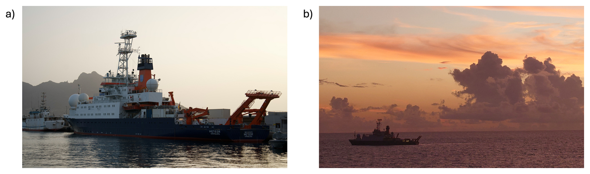
Figure 1 FS Meteor in the port of Mindelo (a; Credit: Philipp Henning), and near the coast of Barbados (b; Credit: Yuting Wu).

2.1 Track

As FS Meteor traveled westward from Cape Verde to Barbados, it also performed north-south excursions to sample near the northern and southern edges of the ITCZ, as shown in Figs. 2 and 3. In Fig. 3, FS Meteor's track shows meridional excursions, which can be divided into three stages in which the longitudinal movement is small compared to the latitudinal one. During the first stage from 16 August to 1 September, FS Meteor deployed two gliders, a WireWalker, and a drift buoy on 18 August near a mooring at 11.5° N and 23° W of the Prediction and Research Moored Array in the Tropical Atlantic (PIRATA; Servain et al., 1998). This deployment is the first process study area (Figs. 2c, 3b). FS Meteor navigated southward until 23 August, then steamed northward until 28 August, when additional instruments and personnel were collected in Praia, Cape Verde. FS Meteor then again headed south and recovered the oceanographic instruments after their 11 d deployment on 29–30 August. FS Meteor continued heading south until 1 September and then turned to travel west along a latitude of 8.5° N.

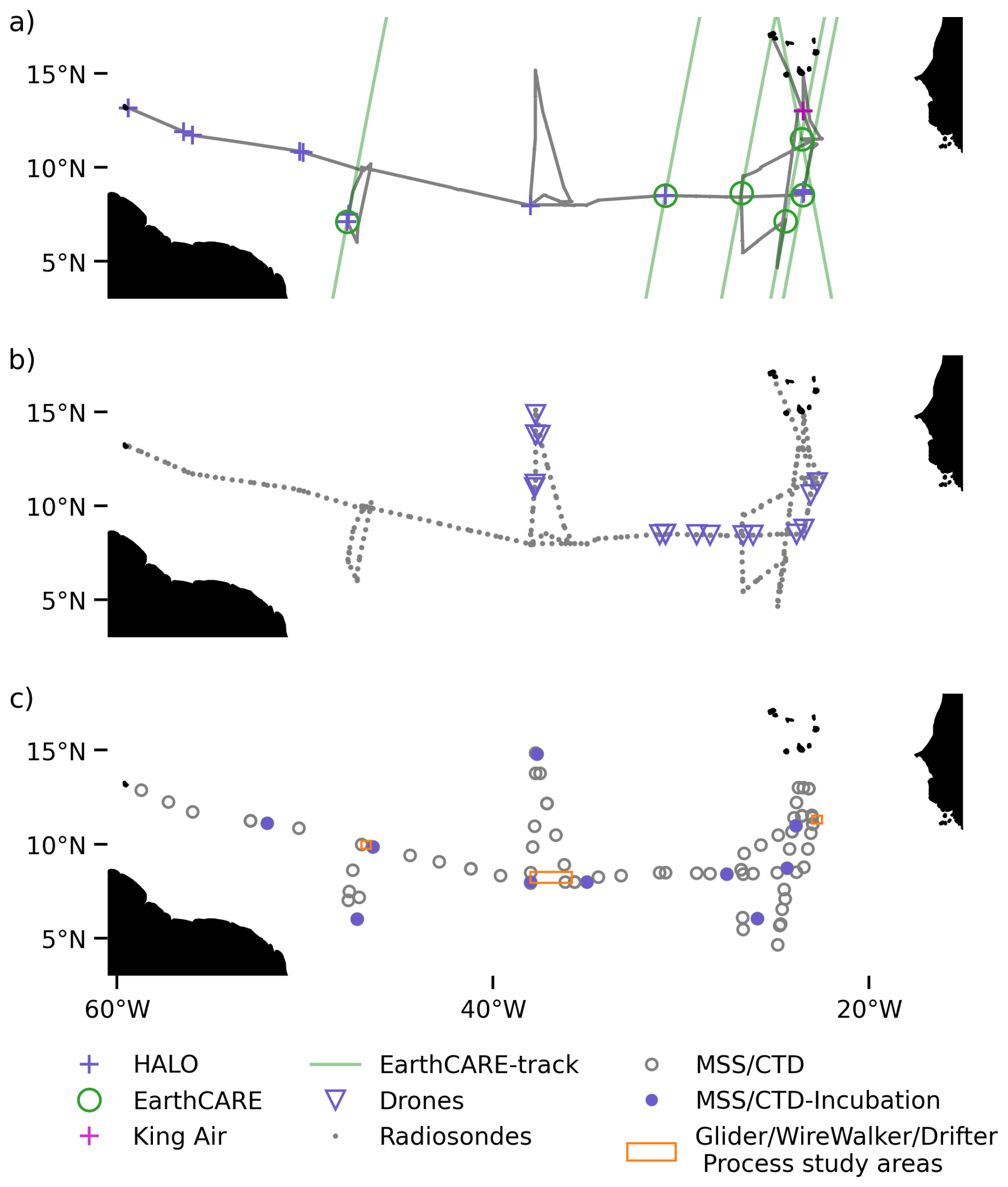
Figure 2 (a) FS Meteor's trajectory during the BOWTIE campaign (gray solid line) and intersection with HALO (blue crosses) and King Air (magenta crosses) flights. EarthCARE tracks (green line) overpassing FS Meteor's trajectory are shown with green circles. (b) Radiosonde launch locations are shown with gray dots, and locations where unmanned aerial vehicles (aerial drones) were deployed are shown with blue triangles. (c) Conductivity-temperature-depth-oxygen (CTDO) measurement locations are shown with gray unfilled circles, and CTDO measurements that included biology samples are shown with blue-filled circles. The areas that gliders, WireWalkers, and drifters sampled are enclosed by orange rectangles, and they are referred to as process study areas.

After continuing a westward trajectory for several days, the second stage of north-south excursion occurred near a longitude of 38° W between 6 and 11 September. After deploying three gliders in the second process study area, the WireWalker, and a drift buoy (Figs. 2c, 3e) near a PIRATA mooring at 8° N and 38° W on 6 September, FS Meteor navigated northward until 9 September. After 9 September, FS Meteor returned southeastward, arriving at 8° N and 36° W on 11 September. The 2° of longitudinal difference between the initial and the end of the second stage (Fig. 2c) occurred because the deployed oceanographic instruments were displaced eastward by the North Equatorial Countercurrent. FS Meteor then headed northwest on 12 September.

The third and final stage of north-south excursion occurred near a longitude of 47° W from 15 to 18 September. On 15 September, two gliders, the WireWalker, and a drift buoy were deployed in the third and final process study area at 10° N and 47° W (Figs. 2c, 3g). FS Meteor then followed a southward trajectory until 6° N, where it arrived on 17 September. FS Meteor then returned northward to recover the oceanographic instruments on 18 September (Fig. 2c) at 10° N and 46.5° W. This was the last meridional excursion for FS Meteor. After this point, FS Meteor headed northwest until it reached Barbados on 23 September.

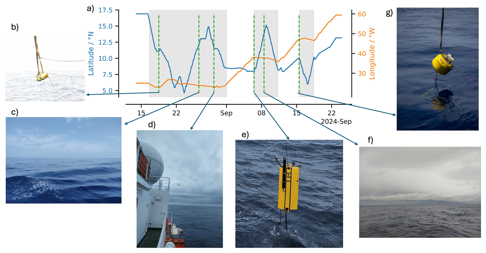
Figure 3 (a) FS Meteor's trajectory in the BOWTIE campaign. Grey areas show periods in which FS Meteor mostly traveled in a north-south direction. (b) Glider being launched on 18 August (Credit: Philipp Henning). (c) Photo taken on 26 August, during a doldrum event, (d) Photo taken on 29 August, during a strong wind regime. (e) Launch of the WireWalker on 6 September. (f) Photo taken on 8 September, the day that a precipitation gust-front occurred. (g) WireWalker being launched on 15 September.

2.2 Stations

Stations are defined as time periods during which a specialized instrument was deployed to perform measurements. The term may also refer to the specific time at which an instrument was launched. Instrument stations indicate that these instruments did not operate continuously through the campaign. For atmospheric measurements, this applies to radiosondes, microtops, and aerial drones. The launch times of radiosondes and the deployment times of aerial drones are recorded, and their locations are shown in Fig. 2b. For ocean measurements, the conductivity-temperature-depth-oxygen sensor (CTDOs), microstructure profiling system (MSS), the gliders, the drift buoy, the WireWalker, the plankton bottle nets, the UVP camera, and nutrient measurements are classified as station-based observations. CTDO measurements required the ship to remain stationary. At selected CTDO stations, additional instruments – such as those for nutrient measurements, the UVP camera, and plankton bottle nets – were also deployed (Fig. 2c). In contrast, the MSS measurements required the ship to move slowly with a small displacement. The location of the MSS measurements are shown in Fig. 2c. Gliders, drift buoys, and the WireWalker are autonomous instruments that were deployed for extended periods and subsequently recovered. During BOWTIE, these platforms were deployed at three distinct locations, referred to as process study areas (Figs. 2c, 3b, e, g).

During CTDO stations, aerial drones were also deployed. Moreover, some of the radiosonde deployments also coincided with CTDO and MSS stations. To take advantage of simultaneous measurements, the BOWTIE collection includes records of the time that CTDO, MSS, radiosondes, and aerial drones were deployed and the time the measurements finished (https://doi.org/10.82246/bafybeianebwhw4uzkqnaekl5 kyoau7hubxaens7azrftgqtz2mccciejle, Segura and Wing, 2026). The information on the time when CTDO and MSS were conducted, as well as the time when aerial drones were deployed, is included in YAML files (https://doi.org/10.82246/bafybeiekpjsfkslf2drgqtigah 7a2y33zuzv6tjlrwgsxqv6plwebbnr5m, Segura, 2026b). This allows the user to easily select data from other simultaneous measurements, e.g., radiosondes.

2.3 BOWTIE and ORCESTRA's sub-campaigns

BOWTIE was closely coordinated with four other sub-campaigns of ORCESTRA, both through measurements conducted from the same platform and through coordinated observations across multiple platforms. PICCOLO (Process Investigation of Clouds and Convective Organization over the Atlantic Ocean) and STRINQS (Soundings and TuRbulent eddy measurements in the ITCZ with a Network of QuadcopterS; Stevens et al., 2026) operated alongside BOWTIE aboard FS Meteor, complementing the ship-based observing system with additional radar and aerial drone measurements. PERCUSION (Persistent EarthCARE Underflight Studies of the ITCZ and Organized Convection) and CELLO (Cloud and EarthCARE caL/vaL Observations) operated from independent airborne platforms, with their observations coordinated with FS Meteor and EarthCARE overpasses. These two forms of collaboration are described separately below.

2.3.1 PICCOLO and STRINQS

As part of the ORCESTRA campaign, BOWTIE coordinated efforts on board FS Meteor with two other sub-campaigns, PICCOLO and STRINQS. PICCOLO installed the Colorado State University Sea-Pol radar (Rutledge et al., 2019) on FS Meteor to measure precipitation and hydrometeor properties of convective storms. Sea-Pol operated continuously during the trajectory of FS Meteor. STRINQS used unmanned aerial vehicles to sample the thermodynamics and dynamics in the lowest 1.5 km of the atmosphere with fine temporal and vertical resolution. The primary objective of STRINQS was to demonstrate the employability of aerial drones from a research vessel to characterize the state of the atmospheric boundary layer in high-resolution. Aerial drones were deployed at 17 dedicated stations during the FS Meteor's trajectory as shown in Fig. 2b. Due to technical problems, the aerial drones were not deployed after 9 September.

2.3.2 PERCUSION and CELLO

BOWTIE coordinated measurements with the PERCUSION and CELLO sub-campaigns of ORCESTRA (Stevens et al., 2026) and EarthCARE satellite overpasses, as illustrated in Fig. 2a. In total, six overpasses by the EarthCARE satellite were coordinated during BOWTIE. For more details, refer to Klocke et al. (2026c).

The PERCUSION campaign employed the German research aircraft HALO to conduct measurements in and across the ITCZ. In addition to in situ observations of thermodynamic variables and wind, HALO was equipped with an extensive suite of passive and active remote sensing instruments, including a 35 GHz radar and a high-spectral-resolution water vapor DIAL lidar. The campaign featured circular flight patterns with extensive dropsonde deployments to characterize mesoscale vertical motion. HALO operated from Sal (Cape Verde) in the eastern tropical Atlantic during the first phase and from Barbados in the western tropical Atlantic during the second phase of the PERCUSION campaign. In total, 17 overpasses and 7 additional close approaches to FS Meteor were achieved in coordination with BOWTIE in 10 d between 16 August and 23 September. Beyond its scientific objectives, PERCUSION emphasized a comprehensive validation of the EarthCARE mission (Groß et al., 2026).

The CELLO campaign focused primarily on the validation of EarthCARE retrievals. Led by a Norwegian initiative, it utilized the Romanian INCAS King Air aircraft operating from Praia (Cape Verde) to perform in situ measurements of aerosols, clouds, and precipitation. Flights were conducted along the EarthCARE ground track. Three coordinated overpasses of FS Meteor were conducted. For more information about the coordination between BOWTIE and both PERCUSION and CELLO, refer to Klocke et al. (2026c).

To facilitate the selection of data acquired during coordinated measurements with PERCUSION and CELLO, a YAML file was created to document the timing of these events. Overpasses above FS Meteor were coordinated with EarthCARE, King Air aircraft, and HALO aircraft. In addition, certain coordinated flight patterns positioned FS Meteor within circular flight tracks executed by HALO. All coordination events and their corresponding metadata are also compiled in a CSV file (https://doi.org10.82246/bafybeianebwhw4uzkqnaekl5 kyoau7hubxaens7azrftgqtz2mccciejle, Segura and Wing, 2026).

3 Instrumentation and processing

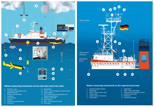
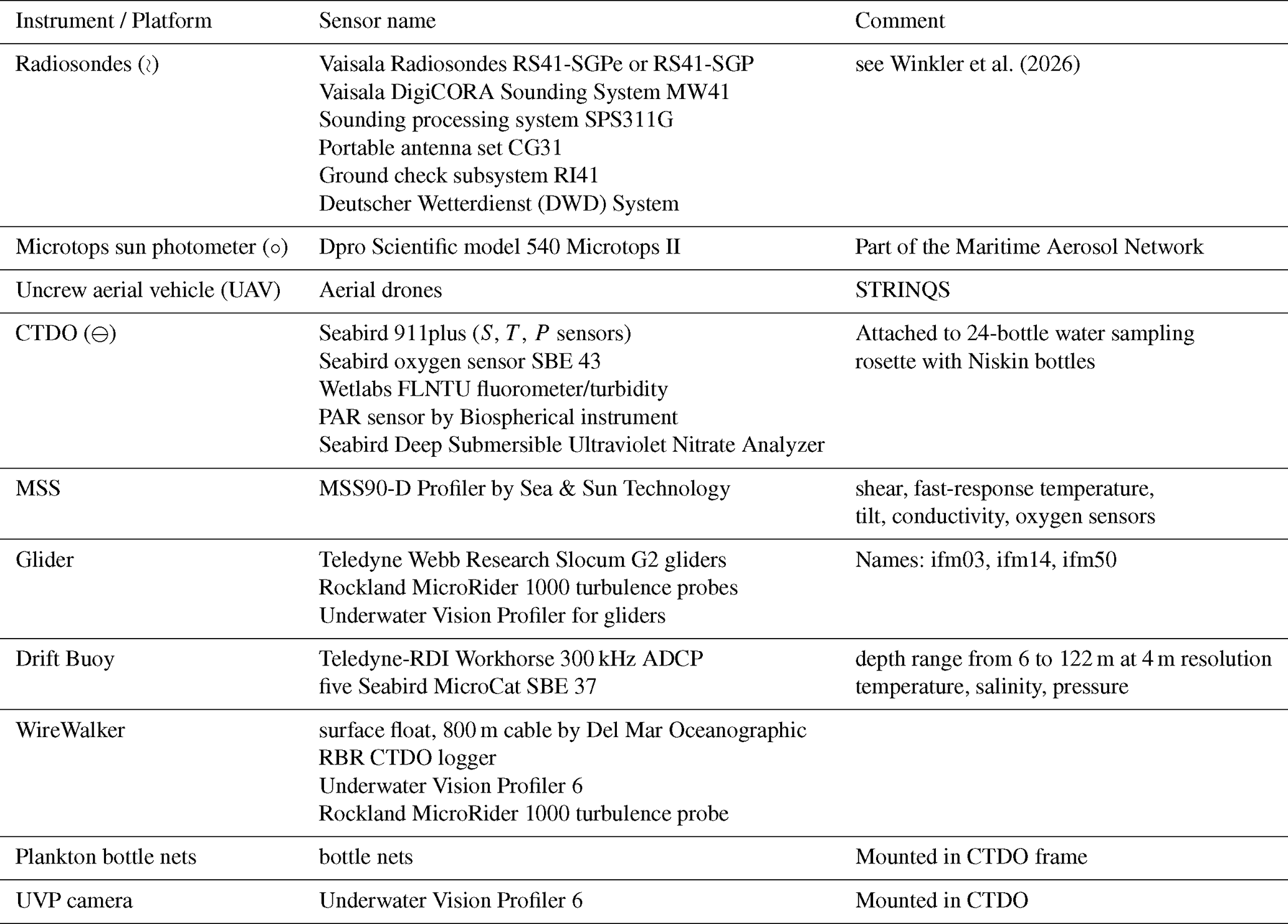
To accomplish BOWTIE's objective, continuous measurements of the atmosphere and ocean were made using 29 instruments (Tables 1, 2 and  3), of which 23 were a BOWTIE contribution, 4 are permanent instruments onboard FS Meteor, and one each were contributed by PICCOLO and STRINQS. Figure 4 shows a schematic of the instruments used in BOWTIE and their location on the ship. Many instruments operated continuously, but discrete measurements of both the ocean and atmosphere were also taken by 11 instruments during stations, detailed in Fig. 2b, c, and described in Sect. 2.2.

Figure 4 Schematic of the instrumentation used in BOWTIE and its placement on the ship.

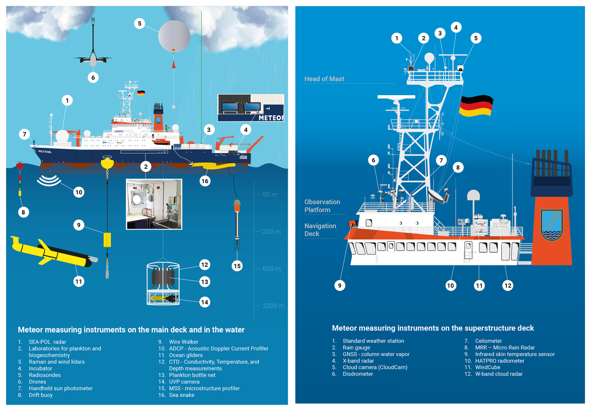
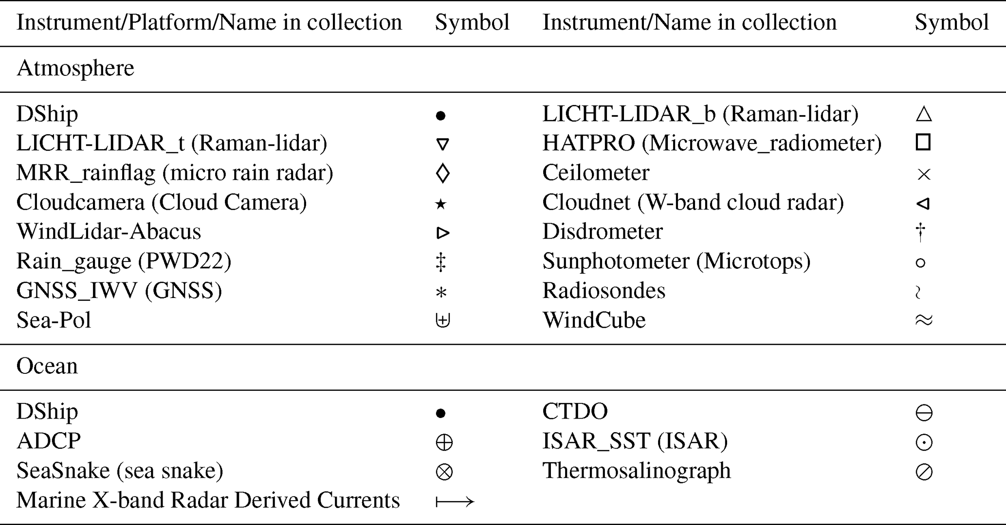
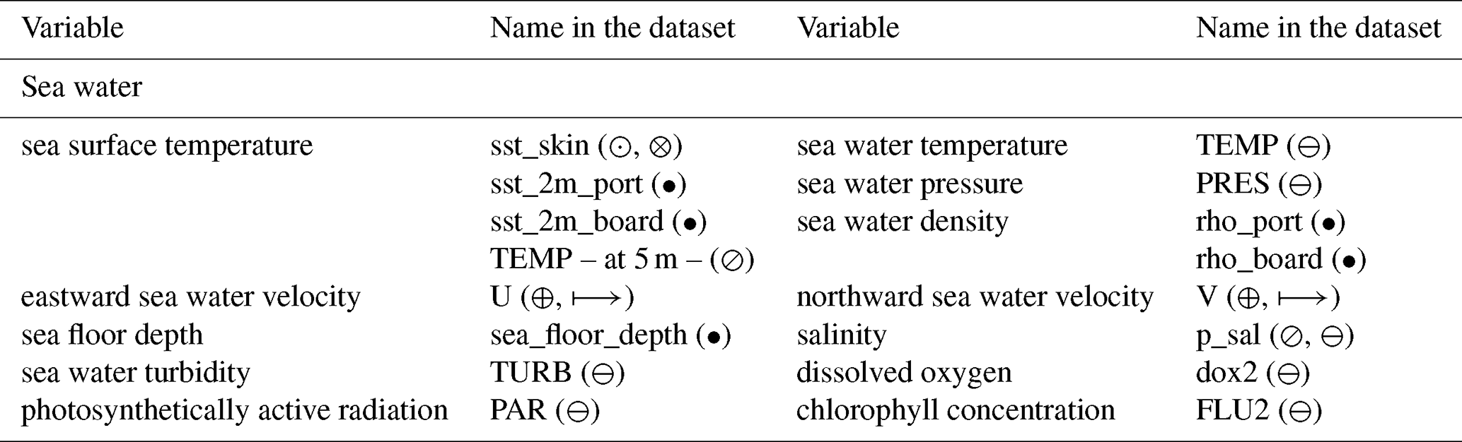
In the final BOWTIE dataset (https://latest-orcestra--campaign-org.ipns.dweb.link/products/METEOR/, last access: 24 April 2026), datasets are generally named after the corresponding instrument, with a few exceptions as noted in Table 1. For clarity, each instrument is assigned a specific marker in this table. Table 2 shows instruments taking continuous measurements, while Table 3 shows instruments deployed in selected stations (Sect. 2.2). Tables 2 and 3 also display specific details of sensors and specific comments. The variables are organized as follows: time and position variables are listed in Table 4, ship orientation variables in Table 5, atmospheric variables in Table 6, and oceanic variables in Table 7. The variables shown in Table 6 and Table 7 represent only a subset of the complete dataset. For a comprehensive overview of all available variables, please refer to the ORCESTRA data browser (https://browser.orcestra-campaign.org, last access: 24 June 2026). In the following, we briefly describe the instruments.

Table 1 Name of the data set in the catalog https://latest-orcestra--campaign-org.ipns.dweb.link/products/METEOR/ (last access: 24 April 2026) and the associated symbol. The name also represents the instrument or platform used during the campaign. If not, the name of the instrument or platform is indicated in parentheses. The exception is DShip, which represents a collection of instruments (see Sect. 3).

3.1 Permanent instruments – Davis Ship System

The Davis Ship System (DShip) includes data from standard meteorological instruments as well as the ship's position, heading, roll, pitch, and heave, referred to as ship orientation. Data was extracted from the ship server using the Python package shipspy (Köhler, 2024). The extracted DShip data has a temporal resolution of 1 min.

3.1.1 Meteorological data

The Ship's Meteorological Office is a permanent institution on the FS Meteor and is operated by the German Weather Service. One of its countless tasks is the continuous measurement of meteorological parameters. An extensive number of measuring instruments are available for this purpose (see Table 1 with symbol •). The weather station provides measurements of wind direction and speed with a resolution of 0.1°; 0.1 m s⁻¹ (2D Ultrasonic Anemometer), respectively; air temperature with a resolution of 0.1 K (EE33); relative humidity with a resolution of 0.1 %; air pressure with a resolution of 0.1 hPa (PTB220), and precipitation (SRM450, Thies, and PWD22). Shortwave (Pyranometer CM11) and longwave radiation (Pyrgeometer CG4) are measured, as well as water temperature (Pt 100 type 2020).

The meteorological measurement data are processed on the meteorological computer located in the ship's meteorological office. The collection, analysis, quality control, and storage of measurements are conducted on this system, which is then fed into the DShip on-board data network.

3.1.2 Ship orientation

The navigation data is the record of two fiber-optic gyrocompasses (Navigat X MK1 and Navigat 2100) and the integrated system Seapath 320+ (see Table 1 with symbol •). Those instruments comprise the navigation system. The two gyrocompasses measure the ship's pitch, roll, and heading. The Navigat 2100 is the principal sensor, and in case of failure, the Navigat X MK1 is used. The Seapath 320+ additionally uses the motion unit MRU 5 and two GPSs antennas to provide highly accurate pitch, roll, heading, and heave of the ship. The MRU 5 sensor is installed at the center of gravity of the ship.

3.1.3 Pure Sea-water system

A thermosalinograph (TSG) is an automated sea near-surface temperature and salinity measurement system using a water intake (see Table 1 with symbol ⊘). Two TSG systems are permanently installed on FS Meteor and are operated in parallel. System 1 draws water from the port side while system 2 draws water from the starboard side of the vessel. Both water intakes are located 5 m below the water line, approximately 4 m behind the bow of the vessel on each respective side of the hull. Each system consists of a conductivity cell with an internal temperature sensor, an external temperature sensor, and a debubbler that removes air bubbles from the input water stream. The external temperature sensors are mounted on the water inlets. Data are logged every ten seconds.

During the cruise, both systems showed acceptable flow speeds between 48.5–56 L min⁻¹. In post-processing, the temperature and salinity data from the TSG were calibrated against CTDO profile data taken during the cruise and salinity measurements from daily water samples drawn from the TSG flow and analyzed with a Guildline Autosal salinometer on board. Quality control, post-processing, and data publication were carried out by the Deutsche Allianz Meeresforschung Underway data project. For data availability and a detailed data processing report, the reader is referred to Schlundt et al. (2025). The final thermosalinograph data is not part of the DShip data, being a separate data set.

3.2 Specialized instrumentation for BOWTIE

In addition to the instruments permanently installed on FS Meteor, the ship was equipped with specialized instrumentation to target BOWTIE's scientific questions. These were installed in Mindelo before departure and removed from the ship after the cruise. We distinguish between instruments measuring in the atmosphere or the ocean, continuously measuring instruments, instruments measuring at discrete intervals during stations, or autonomous instruments deployed for several days before retrieval.

3.2.1 Continuous measurements of the atmosphere

• Raman lidar (▿, △): Manufacturer/developer: Max Planck Institute for Meteorology (MPI-M); type/model: Raman lidar; measured quantities: aerosol backscatter and extinction, depolarization, temperature, water vapor, and cloud-base height; wavelengths: 355, 532, and 1064 nm; measurement range: up to 29 km a.s.l. under clear-sky conditions.

  The MPI-M Raman lidar provides continuous vertical profiles of atmospheric properties. Elastic backscatter measurements at 355, 532, and 1064 nm provide information on cloud-base height and the vertical distribution of aerosols, while depolarization measurements provide information on non-spherical particles such as ice crystals and mineral dust. The backscatter in off-wavelength Raman frequencies near the 355 and 532 nm channels are used to retrieve quantitative profiles of aerosol extinction, temperature, and water vapor. Under clear-sky conditions or thin clouds, profiles can extend to approximately 29 km above sea level; in the presence of optically thick clouds, reliable measurements are generally limited to below the cloud base. Measurements were stopped during rain. Temperature and water-vapor measurements were calibrated against radiosondes during the cruise, while backscatter was calibrated after the cruise using clear-sky periods. Depolarization measurements were not calibrated.

• Microwave radiometer (LIMHAT; □): Manufacturer: Radiometer Physics GmbH (RPG); type/model: RPG-HATPRO Generation 5; measured quantities: microwave brightness temperature and retrieved temperature and humidity profiles, integrated water vapor (IWV), and liquid water path (LWP); frequency ranges: 22.23–31.4 GHz (water vapor absorption lines) and 51.26–58.0 GHz (oxygen absorption lines), with seven channels in each band; installation height: 15.8 m above sea level.

  The microwave radiometer, named LIMHAT, is a passive remote-sensing instrument that measures atmospheric microwave emission in 14 channels around the water-vapor and oxygen absorption lines. A retrieval developed using ERA5 data over the tropical and subtropical Atlantic provides profiles of humidity and temperature as well as IWV and LWP. Reliable retrievals are limited to non-rainy conditions.

  During BOWTIE, LIMHAT was installed on the starboard side of the navigation deck to minimize sea-spray contamination. The instrument operated predominantly in zenith-pointing mode. Every 15 min, a two-minute atmospheric boundary-layer scan was performed at elevation angles of 90, 30, 19.2, 14.4, 11.4, 8.4, 6.6, 5.4, 4.8, and 4.2°. These off-zenith observations (<90°) improved the accuracy of temperature retrievals within the lowest approximately 1.5 km. The same instrument was operated aboard FS Meteor during EUREC⁴A (Schnitt et al., 2024). LIMHAT was calibrated before the cruise according to the manufacturer's guidelines.

• W-band cloud radar (LIMRAD94; ⊲): Manufacturer: Radiometer Physics GmbH (RPG); type/model: RPG-FMCW-94-DP; measured quantities: radar reflectivity, Doppler velocity, Doppler spectrum width and skewness, and cloud boundaries; temporal resolution: 2 s; range resolution: 14–55 m; frequency: 94 GHz (radar) and 89 GHz (passive radiometer); measurement range: approximately 0.1–12 km; installation height: 15.8 m a.s.l.

  LIMRAD94 is a bistatic frequency-modulated continuous-wave (FMCW) Doppler cloud radar (Küchler et al., 2017). Its 3.2 mm wavelength is sensitive to cloud droplets, ice particles, drizzle, and raindrops. Different chirp programs were used during BOWTIE to obtain vertical profiles between approximately 100 m and 12 km. Radar reflectivity, mean Doppler velocity, spectral width, and skewness are derived from the measured Doppler spectra. Under non-rainy conditions, or during light precipitation and moderate IWV, the radar can generally penetrate the full cloud layer. Heavy precipitation and high IWV can strongly attenuate the signal and limit observations of higher cloud layers.

  The radar was installed on the starboard side of the navigation deck in a two-axis cardanic stabilization platform to minimize contamination of Doppler velocities by ship motion (Kalesse-Los et al., 2023). The platform allows free motion of up to ±20° in two directions and uses 150 kg of ballast to limit oscillations. Radar attitude was measured by the internal accelerometer at approximately 0.2 Hz with an accuracy of 0.02° built into the radar itself and by an additional motion sensor combining accelerometer, gyroscope, and magnetometer measurements at 20 Hz (Madgwick, 2010). The performance of the stabilization was evaluated by periodically fixing the radar during the cruise. Misalignment angles of the radar from vertical were compared with misalignment angles from vertical measured in the center of rotation of the ship. It was found that the motion-stabilization platform nearly doubled the fraction of misalignment angles below 0.5° from zenith-pointing to 41 % frequency of occurrence. Radar misalignment from zenith below 1° was reached during 74 % of the time.

  Heave-induced Doppler shifts were corrected during post-processing following the approach of Kalesse-Los et al. (2023) and Acquistapace et al. (2022), applied directly to the unaveraged Doppler spectra. Additional cloud radar processing included filtering of clutter and ghost echoes and unfolding of Doppler spectra before Cloudnet processing (described in Sect. 3.3). The radar was calibrated before the cruise according to the manufacturer's instructions.

• Micro Rain Radar (MRR; ◊): Manufacturer: METEK Meteorologische Messtechnik GmbH; type/model: MRR-PRO; measured quantity used during BOWTIE: near-surface precipitation occurrence; temporal resolution: 10 s; range resolution: 10 m; frequency: 24 GHz; measurement range: 126 m–1.4 km; installation height: 20.66 m a.s.l.

  The MRR-PRO is a compact FMCW Doppler radar designed to measure precipitation profiles (Peters et al., 2005). On a stationary or stabilized platform, Doppler spectra can be used to retrieve quantities such as rain rate and drop-size distributions. During BOWTIE, however, the MRR was neither motion-stabilized nor vertically pointing because an obstruction required the instrument to be tilted by 7°. Consequently, ship-motion effects could not be adequately corrected, and quantitative profile retrievals were not used. Instead, the MRR data were used to provide a near-surface rain flag based on reflectivities exceeding 3.1 dBZ in the fourth range gate at 156 m. This type of measurement is not affected by the MRR tilting or by not having a stabilizing platform. The lowest three range gates were discarded because of artifacts. The MRR was not calibrated.

• Ceilometer (×): Manufacturer: Lufft; type/model: CHM 15k; measured quantities: cloud-base height, atmospheric boundary-layer height, penetration depth, and vertical visibility; temporal resolution: 10 s; wavelength: 1064 nm; measurement range: up to 15 km; installation height: 20.66 m a.s.l.

  The CHM 15k ceilometer is an optical remote-sensing instrument based on a YAG solid-state laser. It detects up to three cloud layers and can observe high-level and cirrus clouds within its approximately 15 km operating range. The ceilometer was installed on the observation deck and was not calibrated during BOWTIE.

• All-sky cloud camera (⋆): Manufacturer/developer: custom-built system; type/model: Mobotix S15D camera with B016 fisheye lens; measured quantity: full-sky imagery; temporal resolution: 10 s; image resolution: 1280×960 pixels; field of view: 180° fisheye.

  The all-sky camera consists of a Mobotix S15D camera equipped with a B016 fisheye lens and mounted in an outdoor housing. Full-sky images were recorded in JPEG format every 10 s and transferred to a network-connected computer, where they were archived in daily files for subsequent processing. The cloud camera was not calibrated.

• Sea-Going Polarimetric Radar (Sea-Pol; ⊎): Manufacturer/developer: Colorado State University (CSU); type/model: Sea-Pol scanning polarimetric C-band radar; measured quantities: radar reflectivity, differential reflectivity, differential phase, correlation coefficient, and Doppler velocity; sampling: scanning strategy comprising multi-elevation Plan-Position-Indicator (PPI), Range-Height-Indicator (RHI), surveillance, and quasi-vertical scans; frequency: 5.65 GHz; wavelength: approximately 5 cm; beam width: 1°; measurement range: 120 km at high resolution and up to 245 km at lower resolution.

  Sea-Pol is a scanning polarimetric radar designed to observe the kinematic and microphysical structure of precipitation (Rutledge et al., 2019). Its 4.3 m antenna and C-band transmitter provide high-resolution polarimetric measurements of precipitation. The measured radar variables are used to characterize hydrometeors, convective structure, and atmospheric flow and to derive products including precipitation rate and hydrometeor classification. An inertial navigation unit measures ship motion and continuously commands the antenna positioner to stabilize the radar scanning plane. The deployment of Sea-Pol on the FS Meteor was supported by the US National Science Foundation (NSF) through the PICCOLO campaign.

  During PICCOLO as part of the BOWTIE cruise, the scanning strategy combined fixed and user-selected scans. Fixed scans included a 245 km surveillance scan at 0.5° elevation, PPI scans providing volumetric coverage to 120 km, and a quasi-vertical profile at 45° elevation. User-selected scans included RHI scans at selected azimuths and additional volume scans to coordinate observations with other platforms. More details on the scanning strategy, processing techniques, and data products can be found at https://seapol.colostate.edu/data/PICCOLO/qc_data/level4/PICCOLO_Sea-Pol_readme.pdf, (last access: 24 April 2026).

  During 16–28 August, Sea-Pol was restricted to single-polarization measurements because of a failed component. Following its replacement on 28 August, dual-polarization observations were obtained for the remaining 28 d of the cruise. Calibration after installation aboard FS Meteor included transmitter-power measurements, internal receiver calibration, alignment of the inertial navigation unit with the ship heading, and solar-pointing verification of antenna offsets. An azimuth pointing offset introduced after the solar verification was corrected during post-processing.

• Disdrometers (†): Manufacturer: OTT Hydromet GmbH; type/model: PARSIVEL (PARticle SIze and VELocity) optical disdrometer; measured quantities: drop-size distribution, particle fall velocity, and precipitation rate; temporal resolution: 1 min; installation height: 20.66 m a.s.l.

  Two PARSIVEL optical disdrometers (Löffler-Mang and Joss, 2000) were installed on the observation deck with their optical sampling paths oriented perpendicular to each other. Disdrometers are labeled DSD_METEOR1 and DSD_METEOR2 in the BOWTIE dataset. The sampling path of DSD_METEOR1 has a bow-stern direction, and the sampling path of DSD_METEOR2 has a port-starboard direction. This alignment of the two disdrometers follows the recommendations of the Marine ARM GPCI Investigations of Clouds (Kollias and Bartholomew, 2016). Measurements of rainfall intensities, particle size distribution, and particle velocities can be affected by wind direction, wind speed, and ship motion (Yuter and Parker, 2001). This is because of turbulence generated by the ship structure (Yuter and Parker, 2001) and instrument (Friedrich et al., 2013a) structure in the wind field.

  Quality control was performed separately for each instrument using a procedure adapted from the 2022 Prediction of Rainfall Extremes Campaign in the Pacific (PRECIP; details of PRECIP can be found at http://precip.org/, last access: 24 April 2026). Drop-size distributions were flagged when observed fall velocities were outside 0.5–1.5 times the expected velocity–diameter relationship of Brandes et al. (2002), thereby identifying contamination by unusually large drops and strong winds (Friedrich et al., 2013b, c). A merged precipitation-rate product was constructed after quality control by selecting the maximum rain rate measured by the two instruments at each time step. Disdrometers were new, and no calibration was conducted.

• Wind lidar Abacus (⊳): Manufacturer: Abacus Laser; type/model: Litra S/S+ Module; measured quantity: line-of-sight wind velocity; sampling: adjustable pulse repetition frequency of 8–50 kHz; wavelength: 1550 nm; measurement range: approximately 8–14 km, depending on aerosol loading.

  The Abacus wind lidar was integrated into the Raman lidar system for BOWTIE. Its transmitter–receiver unit was mounted on an angularly stabilized platform to maintain an approximately vertical pointing direction during ship motion to retrieve vertical wind. The achievable measurement range depends on atmospheric aerosol abundance. The Abacus wind lidar was calibrated before the campaign.

• WindCube (≈): Manufacturer: Vaisala; type/model: WindCube 200S; stabilization platform: OS4000 Offshore Gyro Stabilization Mount, provided by École Centrale de Nantes; measured quantities: vertical wind profiles and spatial variability of radial wind velocity; sampling: alternating Doppler Beam Swinging (DBS), PPI, and RHI scans on a 10 min cycle; vertical resolution: 25 m in DBS mode; range resolution: 50 m in PPI and RHI modes; installation height: 18.3 m a.s.l.

  The WindCube 200S is a long-range scanning Doppler lidar capable of mapping the three-dimensional wind field. Its nominal range extends to approximately 10 km but depends on aerosol abundance and cloud conditions. During BOWTIE, zenith-pointing measurements typically provided good signal-to-noise ratios to 1–1.2 km, while horizontal scans extended to 6–10 km from the ship.

  The lidar alternated between DBS, PPI, and RHI scans. DBS measurements used four azimuths (0, 90, 180, and 270°) at an elevation of 80°, followed by a vertical beam. Groups of six DBS scans (∼ 75 s) were performed every 10 min, yielding wind profiles with ∼ 15 s temporal and 25 m vertical resolution from 68.4 m a.s.l. upward.

  During the remainder of each 10 min cycle, PPI scans covered an azimuth sector of 10–110° at seven elevation angles between −0.5 and 4°. Three RHI scans were additionally performed at azimuths of 20, 60, and 100°, spanning elevations from −0.5 to 11.5°. The stabilization platform reduced typical pitch and roll from approximately 4 to 0.4° and was thus critical for the PPI scans. During the final part of the cruise, the platform malfunctioned and was disabled; these periods are identified by data-quality flags. The motion-stabilization platform is not critical for DBS wind profiles when averaged over 10 min. However, it's recommended to take into account that unrealistic values could arise. Prior to the cruise and after installation of the Windcube into the stabilization platform, a hard-target calibration is performed to determine the scanner's azimuth/elevation alignment and verify the range calibration.

• Global Navigation Satellite System (GNSS; ∗): Manufacturer: C-Nav/NovAtel; type/model: C-Nav3050 GNSS receiver with NovAtel NAVAN2004T antenna; measured quantity: raw GNSS code and carrier-phase observations, used to retrieve integrated water vapor (IWV); temporal resolution: 30 s.

  Raw GNSS observations from the vessel navigation system were used to retrieve IWV from tropospheric signal-propagation delays. Processing followed the methodology of Bosser et al. (2021, 2022) and used precise point positioning with ambiguity resolution implemented in GipsyX version 2.2 (Bertiger et al., 2020). JPL orbit, clock, phase-bias, and wide-lane products were used for the GPS constellation to estimate receiver position and zenith total delay (ZTD) at 30 s resolution.

  ZTD was estimated using Vienna Mapping Functions 1 (VMF1) and VMF3 a priori delays (Re3data.Org, 2016), with temporal variations constrained by a random walk of 25 mm² h⁻¹. Following outlier screening, ZTD was converted to IWV using the approach of Bevis et al. (1992), ERA5 surface pressure (Hersbach et al., 2020), and weighted mean atmospheric temperature provided by TU Wien (Re3data.Org, 2016).

3.2.2 Station measurements of the atmosphere

• Radiosondes (≀): Manufacturer: Vaisala; type/model: RS41-SGPe (BOWTIE and DWD) and RS41-SGP (PICCOLO); measured quantities: temperature, relative humidity, pressure, position, and derived wind; sampling: eight regular launches per day (3-hourly), supplemented by coordinated launches; ground station: Vaisala MW41 Sounding System with CG31 Portable Antenna Set (BOWTIE).

  A total of 327 radiosondes were launched during BOWTIE, providing 327 ascent and 318 descent trajectories. Of these, 253 launches were contributed by BOWTIE, 35 by PICCOLO, and 39 by the German Weather Service (DWD). Because of the delayed departure from port, the first three radiosondes were launched irregularly while FS Meteor was still in Mindelo harbor and are included in the dataset. Regular 3-hourly launches began on 16 August at 10:50 UTC and continued until the final launch on 24 September at 01:50 UTC. An additional 17 radiosondes were launched in coordination with EarthCARE, HALO, and King Air overpasses.

  Two ground stations, one operated by DWD and one installed by BOWTIE, enabled the 3-hourly launch schedule. Launches were timed approximately 1 h 20 min before the target observation times of 00:00, 03:00, 06:00, 09:00, 12:00, 15:00, 18:00, and 21:00 UTC, such that the balloons reached the upper troposphere near these times, following the DWD protocol. Soundings targeting 00:00, 06:00, 12:00, and 18:00 UTC were performed using the DWD ground station and transmitted to the Global Telecommunication System (GTS) for operational weather forecasting and data assimilation. One of the eight routine daily launches was performed by DWD personnel.

  The BOWTIE ground station consisted of a Vaisala MW41 Sounding System connected to a CG31 Portable Antenna Set and an automatic weather station measuring pressure and temperature. Wind speed, wind direction, and seawater temperature were obtained from the ship's DShip data stream. DShip meteorological data were also used for launches performed with the DWD ground station. Raw radiosonde data were post-processed using the Python package pysonde (Schulz et al., 2024). Radiosondes were new, and no calibration was conducted.

  No specific quality control was performed on the first 50 m of the measurements. In the Level-2 data, temperature frequently decreases by more than the dry adiabatic lapse rate between 10 and 20 m before increasing over the subsequent one to three levels (not shown). The cause is not fully understood but may involve effects of the ship's structure (Yoneyama et al., 2002). We therefore recommend excluding radiosonde measurements below 30 m in the Level-2 data and the first three height levels in the Level-1 data. Further information on quality control, five cases of oscillating balloons, and transmission to the GTS is provided by Winkler et al. (2026).

• Microtops sun photometers (∘): operators/contributors: MPI-M/NASA and IOPAN; measured quantities: column-integrated aerosol and water-vapor properties; sampling: manual measurements under unobscured-sun conditions.

  Handheld sun-photometer measurements were performed manually when the solar disk was not obscured by clouds, allowing observations under both clear and partly cloudy conditions. The measurements provide atmospheric column properties of aerosols and water vapor. Data were submitted to the Maritime Aerosol Network (MAN) of AERONET (http://aeronet.gsfc.nasa.gov/new_web/maritime_aerosol_network.html, last access: 24 April 2026), where measurements and derived products, including aerosol fine-mode fraction, are made available. The sun photometer is calibrated at the NASA Goddard Space Flight Center (GSFC) calibration facility via a transfer calibration procedure between the Microtops and the master Cimel sun photometer at GSFC. The calibration was conducted before the cruise. More information is detailed in Smirnov et al. (2009).

• Aerial drones: type/model: four meteorological quadcopters [please specify model]; measured quantities: temperature, relative humidity, pressure, and three-dimensional wind; sampling: coordinated horizontal and vertical flight patterns during stations; horizontal range: approximately 3 km from the ship; maximum altitude: approximately 1.5 km.

  Four quadcopter drones contributed by STRINQS were deployed for meteorological measurements. Each drone carried sensors for relative humidity, temperature, and pressure, including two independent sets of pressure sensors, as well as a sonic anemometer for three-dimensional wind measurements. The sonic anemometer was mounted on a vertical mast more than 1 m from the propellers to minimize flow disturbance.

  Flight strategies varied among stations depending on the number of drones operating simultaneously and included both horizontal and vertical sampling patterns. Measurements were restricted to periods when FS Meteor was stationary and were generally conducted within approximately 3 km of the ship and up to 1.5 km altitude. Drone operations were most often coordinated with CTDO measurements.

3.2.3 Continuous measurements of the ocean

• Infrared Sea Surface Temperature Autonomous Radiometer (ISAR; ⊙): Manufacturer/developer: ISAR project (https://www.isar.org.uk/, last access: 12 September 2026); type/model: ISAR with Heitronics KT15.85D infrared radiometer; measured quantity: sea-surface skin temperature; accuracy: 0.1 K.

  ISAR is an autonomous infrared radiometer for measuring sea-surface skin temperature. The system uses two reference blackbody cavities to maintain the radiometric calibration of the Heitronics KT15.85D radiometer. It consists of fore-optics, detector and blackbody calibration subsystems, an internal control and data-acquisition computer, an environmental protection system with a storm shutter, and an external RS485 interface for additional atmospheric and oceanographic sensors. The storm shutter prevents measurements during rainy conditions. A detailed description of ISAR is provided by Donlon et al. (2008).

• Sea snake (⊗): Manufacturer/developer: NOAA Physical Sciences Laboratory; type/model: floating near-surface temperature sensor with slow-response thermistor; measured quantity: near-surface (subskin) seawater temperature; sampling: 1 s averages; nominal measurement depth: 0.05 m.

  During BOWTIE, the sea snake was towed from the port side of the midship deck using an outrigger boom, approximately 3 m from the ship's hull. The sensor consists of an exposed slow-response thermistor attached near the end of a floating, air-filled rubber tube, with approximately 30 cm of tubing extending beyond the sensor to keep it submerged. The deployment minimizes contamination by warm water discharged from the ship and heating associated with the hull and engines. Although the installation differs from that described by Fairall et al. (1997), the measurement principle is the same. The thermistor is intentionally deployed within the ship's wake, where mixing around the hull allows the nominally 5 cm-deep sensor to approximate the temperature of the subskin layer beneath the interfacially cooled skin (Fairall et al., 1996, 1997). Its relatively slow response reduces sensitivity to transient air bubbles and brief exposure to air as waves pass the sensor. At night, in the absence of diurnal warm layers, sea snake temperatures are expected to agree with the ship's underway thermosalinograph (TSG) measurements (Gentemann et al., 2009). During BOWTIE, nighttime sea snake measurements agreed with the TSG within 0.002 K; therefore, no correction or calibration was applied.

• Hereon Marine X-band Radar (↦): Manufacturer/developer: Helmholtz-Zentrum Hereon; type/model: Hereon marine X-band radar V3; measured quantities: ocean-surface radar backscatter (amplitude and phase); sampling: continuous acquisition at 40 MHz while the antenna rotates through 360°;

  The Hereon marine radar system (Horstmann et al., 2021) is a high-resolution X-band radar designed for detailed observation of ocean surface physical properties. Operating at 9.4 GHz, it captures both backscatter intensity and phase information, enabling advanced analysis of sea surface dynamics. The radar uses short 50 ns pulses to achieve a spatial resolution of approximately 7.5 m and supports pulse repetition frequencies up to 2 kHz with Vertical-Vertical polarization and a rotating antenna capable of 360° scans at 30 rpm. The data products include surface currents (Lund et al., 2018), significant wave height (Carrasco et al., 2024), wave energy dissipation (Streßer et al., 2022), air-sea interaction (Streßer et al., 2026), as well as individual wave tracking and short-term wave forecasts (Carrasco et al., 2025).

  During BOWTIE, the Hereon marine radar system was configured to generate geolocated backscatter intensity maps, which serve as the basis for deriving relative surface roughness and two-dimensional surface current fields. The surface current retrieval method is based on the linear wave dispersion relation by examining the temporal and spatial evolution of the wave field. Local currents induce Doppler-shifted wave frequencies, which are analyzed to infer surface current velocities, achieving a root-mean-square error of 0.04 m s⁻¹ (Lund et al., 2018).

  The X-band radar systems require the calibration of two key parameters after the installation: the range offset and the azimuth offset. The range offset, or the delay range, accounts for systematic delays introduced by the radar electronics and signal processing chain. This needs to be calibrated to correct the measured range and to get the true position between the target and the radar. The azimuth offset represents the angular difference between the radar reference heading and the vessel heading and is corrected to ensure the proper orientation of the resulting two-dimensional radar images within the geographic coordinate system. Accurate determination of these offsets is essential for the precise retrieval of surface currents. Further details on the radar calibration procedure can be found in McCann and Bell (2018).

• Upper-ocean velocities (ADCP; ⊕): Manufacturer: Teledyne RD Instruments; type/models: 75 and 38 kHz Ocean Surveyor vmADCPs; measured quantity: upper-ocean current velocity; vertical resolution: 8 m (75 kHz) and 32 m (38 kHz); measurement range: 17–750 m (75 kHz) and 53 to > 1600 m (38 kHz).

  Upper-ocean currents were measured continuously throughout the cruise using two vessel-mounted ADCPs. Both instruments were mounted in the vessel's hull approximately 5 m below the waterline. The 75 kHz Ocean Surveyor provided higher vertical resolution, whereas the 38 kHz system achieved greater depth coverage at coarser resolution. To reduce acoustic interference, the 75 kHz transducer was installed at 45° relative to the ship's axis, while the 38 kHz transducer was aligned with the ship.

  Both systems were operated in narrow-band mode to increase depth coverage at the expense of some measurement accuracy (Fischer et al., 2003). High-quality ship position, heading, pitch, and roll data from the vessel's navigation system (Sect. 3.1) were used during processing. Water-track calibrations performed during post-processing yielded temporally stable misalignment angles and gain factors with low standard deviations for both instruments, indicating high data quality (Kopte et al., 2024a, b). Quality control, post-processing, and data publication were carried out within the underway research data project of the German Marine Research Alliance (DAM). Detailed processing information is provided by Kopte et al. (2024c, d).

(Bosser et al., 2021, 2022)Horstmann et al. (2021)

Table 2 Instruments taking continuous measurements in the atmosphere and the upper ocean. The symbols indicate the associated name of the data set as shown in Table 1.

Winkler et al. (2026)

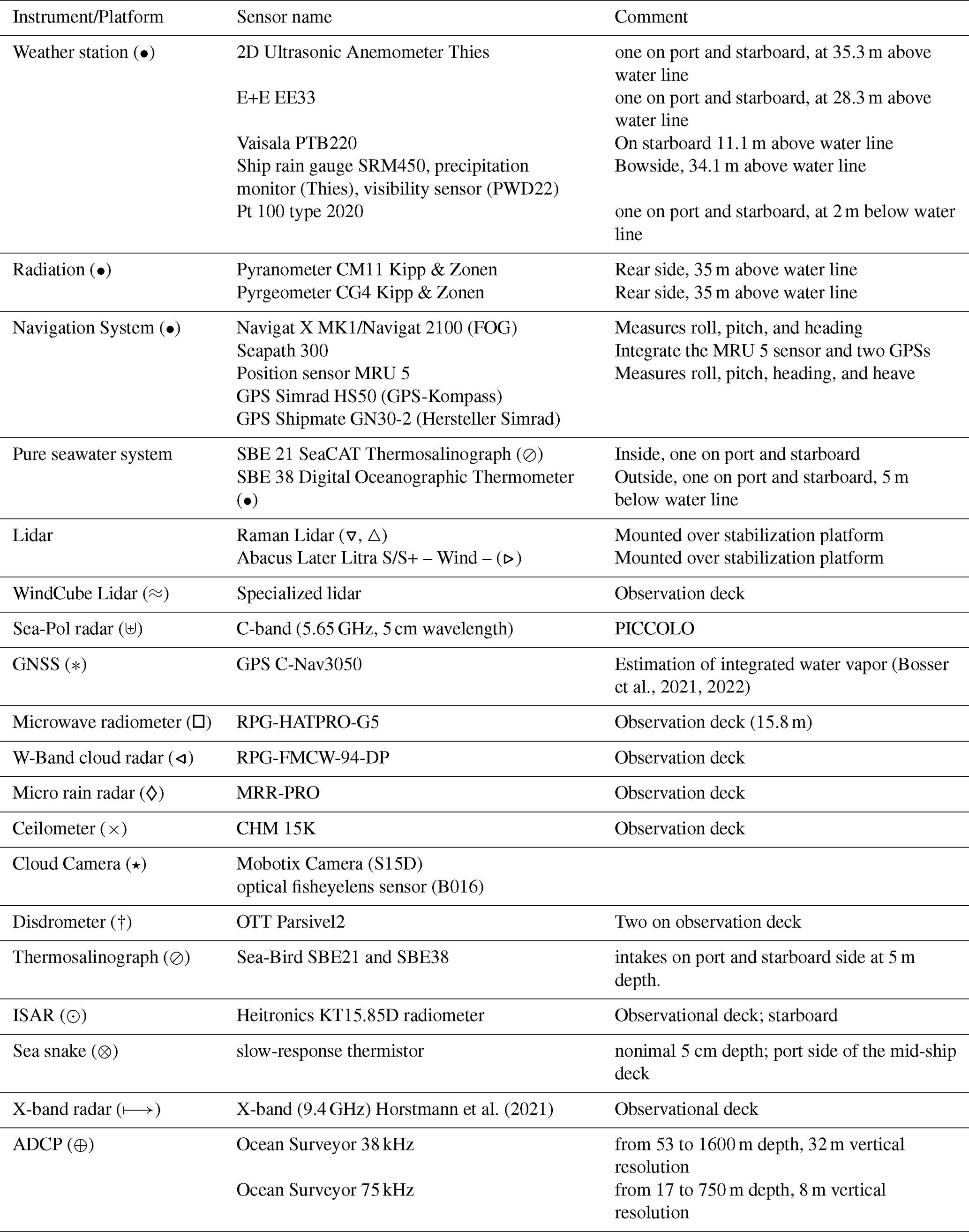
Table 3 Instruments used in stations for taking measurements in the atmosphere and the ocean in specific locations. The symbols indicate the associated name of the data set as shown in Table 1.

3.2.4 Station measurements of the ocean

• Conductivity–Temperature–Depth–Oxygen (CTDO) measurements (⊖): Manufacturer: Sea-Bird Scientific; type/model: SBE 911plus with dual temperature, conductivity, and oxygen sensors; measured quantities: temperature, conductivity, pressure, and dissolved oxygen; processed vertical resolution: 1 dbar.

  The CTDO system was mounted on a 24-bottle rosette equipped with 10 L Niskin bottles; at stations where bottle nets were installed, the number of Niskin bottles was reduced. Water sampling, processing, and calibration followed GO-SHIP recommendations (Swift, 2010; Mctaggart et al., 2010; Uchida et al., 2010). Processing included data conversion, sensor time alignment, creation of bottle files, outlier removal, pressure filtering, conductivity-cell thermal-mass correction, ship-roll and deck-offset corrections, and calculation of derived properties. Conductivity and oxygen measurements were calibrated against salinometry and Winkler titration measurements, respectively. The final downcast data were averaged into 1 dbar intervals.

  Additional sensors mounted on the rosette included a Wetlabs FLNTU fluorometer for chlorophyll a fluorescence and turbidity, a Photosynthetically Active Radiation (PAR) sensor (Biospherical Instruments), and a Submersible Ultraviolet Nitrate Analyzer (SUNA; Sea-Bird/Satlantic). SUNA data were processed following Sakamoto et al. (2009, 2017) and calibrated against nitrate concentrations from discrete water samples. Manufacturer calibrations were applied to the chlorophyll a, turbidity, and PAR measurements.

• Vessel-based ocean turbulence observations: Manufacturer: Sea & Sun Technology; type/model: MSS90-D, S/N 73; measured quantities: turbulent shear, fast-response temperature, hydrography, turbidity, and dissolved oxygen; sampling: [please specify sensor sampling frequencies]; profiling speed: 0.5–0.6 m s⁻¹; typical profiling depth: 150–200 m.

  Vessel-based microstructure profiles were collected before or after CTDO stations to quantify the dissipation rate of turbulent kinetic energy and infer turbulent mixing rates. The loosely tethered MSS consisted of the profiler, a winch with approximately 800 m of cable, and a data interface. The profiler carried three microstructure shear sensors, a fast-response temperature sensor, an accelerometer, two tilt sensors, and lower-response conductivity and temperature (Sea & Sun Technology), pressure (Keller), turbidity (Seapoint), and optical oxygen (Sea & Sun Technology) sensors.

  In total, 243 microstructure profiles were collected. Typically, three profiles extending from the surface to 150–200 m were obtained at each MSS station. During a 15 h station at 13° N, 23°45^′ W on 26–27 August, 54 profiles were collected. The profiler was operated without a protection cage to minimize vibrations during descent. Standard post-processing algorithms (Lueck et al., 2024; Fer et al., 2024) were used to estimate the dissipation rate of turbulent kinetic energy. The sensitivity of the shear sensors were lab-calibrated after the cruise.

• Ocean Gliders: Manufacturer: Teledyne Webb Research; type/model: Slocum gliders (ifm09, ifm14, and ifm50); measured quantities: temperature, conductivity, pressure, oxygen, chlorophyll, turbidity, and ocean microstructure; sampling: profiling missions lasting 3–11 d; maximum profiling depth: 200–700 m, depending on mission.

  Two or three Slocum gliders were deployed in each of the three process-study regions (Fig. 2c) to sample hydrographic, biogeochemical, and turbulent variability at high spatial resolution within the ITCZ. All gliders carried temperature, conductivity, pressure, oxygen, chlorophyll, and turbidity sensors as well as MicroRider microstructure probes (Rockland Scientific). Glider ifm14 additionally carried an optical nitrate sensor (SUNA, Satlantic), while glider ifm50 carried an Underwater Vision Profiler (UVP-6; see below).

  Glider ifm50 sampled the upper 200 m while circling PIRATA buoys at 23° W (first process study area) and 38° W (second process study area) or attempting to maintain position at 10° N, 48° W (third process study area). Glider ifm09 or ifm14 followed the drifting buoy during the process studies, providing turbulence measurements complementary to the buoy velocity observations during the three process study areas. Maximum profiling depths for these missions ranged from 350 to 700 m. A third glider deployed during the second process study followed the WireWalker to provide reference turbulence measurements. The MicroRider probes carried two microstructure shear sensors, two microstructure temperature sensors, a fast-response accelerometer, and a tilt sensor. In total, the gliders collected 2102 hydrographic and 1658 turbulence profiles.

  Temperature, conductivity, and oxygen sensors were calibrated against CTDO profiles collected at the deployment and, if available, recovery position. Additionally, the glider optodes measuring oxygen were lab-calibrated for 0 % and 100 % saturation. Sensitivity of the shear sensors attached to the microstructure probe was lab-calibrated after the cruise.

• Drift Buoy: type/model: drifting buoy with downward-looking 300 kHz ADCP and seven Sea-Bird Microcat sensors; measured quantities: near-surface current velocity, temperature, salinity, and buoy position; measurement depths: ADCP at 3 m; temperature and salinity at 3, 13, 18, 23, 33, 43, and 53 m.

  The drifting buoy was deployed during the three process studies (Figs. 2c, 3b, e, g) to obtain time series of velocity and hydrography within and below the surface mixed layer. These observations targeted processes including near-inertial and internal waves and complemented measurements from the gliders and WireWalker. The seven Microcat sensors were attached to a wire terminating in a 50 kg weight. A GPS receiver recorded the buoy position every second, allowing absolute velocities to be derived from the drifting ADCP measurements. A second GPS receiver with automated Iridium-SBD transmission was used for real-time tracking of the buoy.

  Calibration of temperature and conductivity sensors of the loggers was performed against CTDO data. The loggers were attached to the CTDO rosette prior to the deployment. During these CTDO calibration casts, five 10 min stops in the upper ocean were done at different depths during the upcast to allow the sensors to adjust to ambient water temperature.

• WireWalker: type/model: wave-powered vertically profiling platform; measured quantities: hydrography, ocean microstructure, particles, and plankton; maximum system depth: 1000 m; maximum sampled depth during BOWTIE: approximately 750 m.

  The WireWalker is a freely drifting, wave-powered platform that repeatedly profiles the water column (Pinkel et al., 2011). The system consists of a surface buoy, a weighted steel cable, and the profiling unit. A one-way clamping mechanism causes the profiler to move downward along the wire as waves displace the surface buoy. At the lower end of the cable, a turn-around bumper releases the clamps, allowing the positively buoyant profiler to ascend freely. Measurements are generally collected during the smoother and more uniform upward transit.

  During BOWTIE, the WireWalker was deployed in all three process studies and carried a UVP-6 plankton camera, a microstructure probe, and a conductivity–temperature–depth (CTD) sensor. A fluorescence sensor and an oxygen sensor were additionally installed during the first deployment. All three deployments successfully collected profiles from near the surface to approximately 750 m depth. Calibration was not performed on the CTD installed in the WirWalker because analysis will be based on relative changes rather than absolute values.

• Plankton Bottle Nets: type/model: bottle-mounted plankton net with 20 µm mesh; measured quantity: microplankton abundance and community composition; sampling: one integrated sample per depth interval and deployment; sampling intervals: 0–100, 100–200, 200–300, and 300–600 m.

  Four bottle nets were mounted on the CTDO rosette, with each net replacing two Niskin bottles. Each device consists of a PVC and stainless-steel frame containing a 20 µm plankton net. Sampling was performed exclusively during the CTDO upcast. At the target depth, each bottle net was opened to filter seawater and collect organisms and was subsequently closed to prevent further sampling during ascent.

  Samples were retrieved on board, preserved with Lugol's solution, and prepared for subsequent analysis. Individual casts were conducted entirely during either daytime or nighttime to minimize the influence of diel vertical migration. The samples are used for taxonomic identification and characterization of microplankton diversity, to investigate plankton community composition and its role in the active carbon pump.

• Underwater Vision Profiler (UVP-6): type/model: UVP-6, low-power and high-frequency versions; measured quantities: particles and zooplankton >100 µm; sampling: 1.3 images s⁻¹ (low-power) or approximately 20 images s⁻¹ (high-frequency); camera: 5-MP monochrome camera.

  The UVP-6 is an underwater imaging system for characterizing large particles and zooplankton. The sampling volume is illuminated by a red laser, and images are acquired with a 5-MP monochrome camera. Regions of interest are identified and retained directly by the instrument, reducing onboard storage requirements.

  During BOWTIE, a high-frequency UVP-6 was deployed on the WireWalker, a low-power version on one ocean glider, and an additional high-frequency UVP-6 on the CTDO rosette. Processed UVP-6 data provide particle properties, including size, shape, and solidity, as well as plankton taxonomy and abundance. The UVP-6 cameras were new, and no calibration was performed.

• CPICS: type/model: CPICS underwater imaging system; measured quantities: particles and zooplankton; sampling: approximately 6 images s⁻¹; camera: 12.3-MP color camera; optics: telecentric lens with 0.9× magnification.

  CPICS provides higher-resolution color imagery than the UVP-6, although over a considerably smaller imaged volume. The greater spatial resolution enables more detailed characterization of individual particles and zooplankton. During BOWTIE, CPICS was mounted on the CTDO rosette. A small leak developed after the first few days of operation, preventing further deployments.

• Discrete Water Sampling for Nutrient and Microbial Analyses: Sampling system: Niskin bottles mounted on the CTDO rosette; measured quantities: inorganic and organic nitrogen and phosphorus compounds, primary productivity, nitrogen fixation, phosphonate utilization, microbial community composition, and cell-specific activity; analysis methods: stable-isotope incubations, metagenomic and transcriptomic sequencing, and nanoSIMS.

  Water samples collected with the CTDO rosette were used to determine concentrations of inorganic and organic nitrogen and phosphorus compounds. Incubation experiments with stable isotopes, with and without nutrient supplementation, were used to quantify primary productivity, nitrogen fixation, and phosphonate utilization. Microbial communities were characterized using metagenomic and transcriptomic sequencing, while nanoSIMS measurements were used to determine cell-specific activity of key microbial groups.

3.3 Cloudnet processing

The microwave radiometer and W-band cloud radar were operated by Leipzig University. In combination with data from the Lufft CHM 15K ceilometer operated by MPI-M, the microwave radiometer data and cloud radar data were processed using the Cloudnet processing scheme (Illingworth et al., 2007; Tukiainen et al., 2020) to obtain atmospheric properties in the vertical column above FS Meteor. The Cloudnet processing was done on the Cloudnet data portal (https://cloudnet.fmi.fi, last access: 24 April 2026), where auxiliary information on profiles of atmospheric temperature and pressure from ECMWF-IFS model is available along the ship track. Cloud radar observations were corrected for atmospheric attenuation by water vapor. Cloudnet products include a profile-based target classification separated into pixels containing ice, liquid, aerosol, and precipitation. The temporal resolution of Cloudnet products is 30 s and the vertical resolution is the same as the cloud radar resolution (on the order of a few tens of meters). Cloudnet also provides retrievals of microphysical cloud properties such as liquid water content, ice water content, and effective radius of droplets and ice particles. During the two-minute-long atmospheric boundary layer scans of the microwave radiometer (termed “MWR multiple pointing” times in Cloudnet), Cloudnet does not use the microwave radiometer data and thus labels the liquid water path as “Invalid LWP”, which in turn prohibits the determination of liquid water content (LWC) during the MWR scan times. Using the quality-controlled and heave-corrected radar data (level 1 data), Cloudnet creates a rain detection flag for the W-band cloud radar dataset. Subsequent data analysis revealed that the rain flag is true when the reflectivity in the fourth range gate (at 165 m) exceeds 3.1 dBZ and the Mean Doppler Velocity (MDV) is negative. The dataset resulting from the Cloudnet processing gives a level 2 product. Adding a flag for ghost echoes and strong radar signal attenuation manually results in level 2a data. An additional variable of radar beam misalignment angle from zenith will be added in the level 2b product for a better assessment of the bias induced to MDV observations by horizontal wind speeds.

Table 4 The names of the variables used to indicate time and position, and their respective nomenclature in the data set. All data sets have time, longitude, and latitude as variables. For the other variables, the symbol or symbols next to the name in the data set and between parentheses indicate which data set is used. The symbols are according to Table 1.

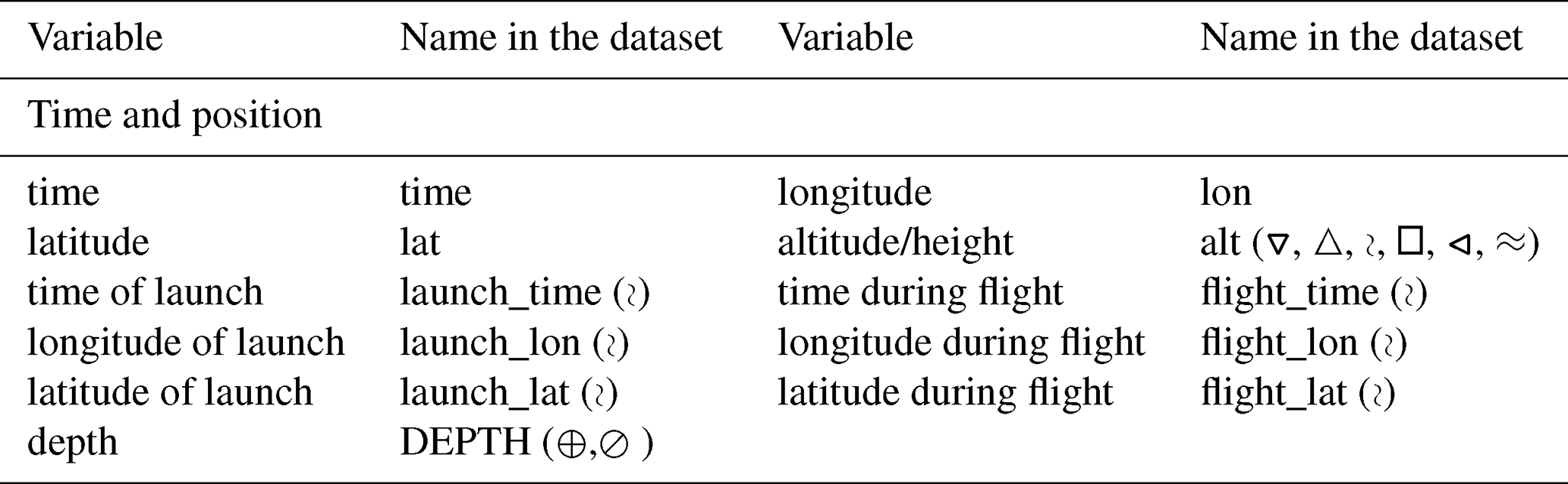
Table 5 The names of the variables used to indicate the ship orientation, and their respective nomenclature in the data set. The symbol or symbols next to the name in the data set and between parentheses indicate which data set is used. The symbols are according to Table 1.

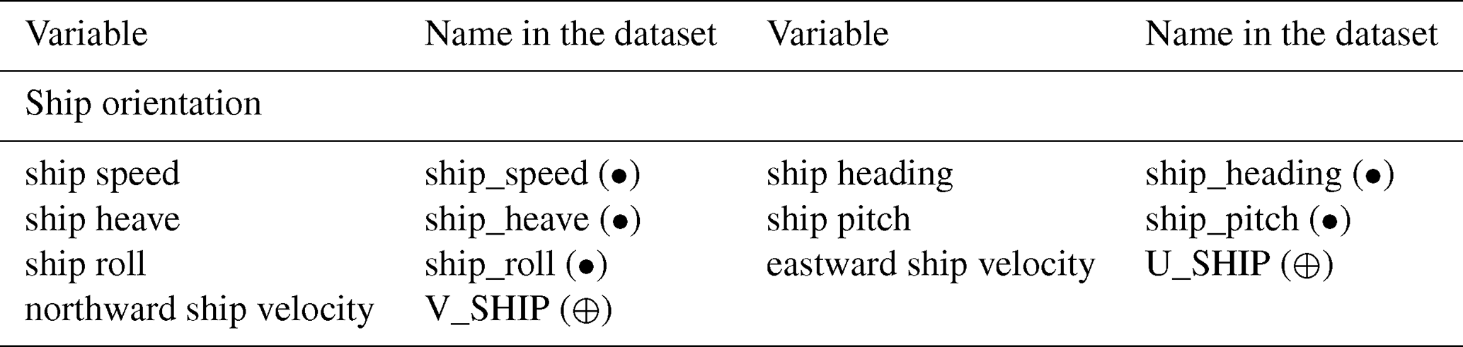
Table 6 The names of the measured atmospheric variables and their respective nomenclature in the data set. The symbol or symbols next to the name in the data set and between parentheses indicate which data set is used. The symbols are according to Table 1.

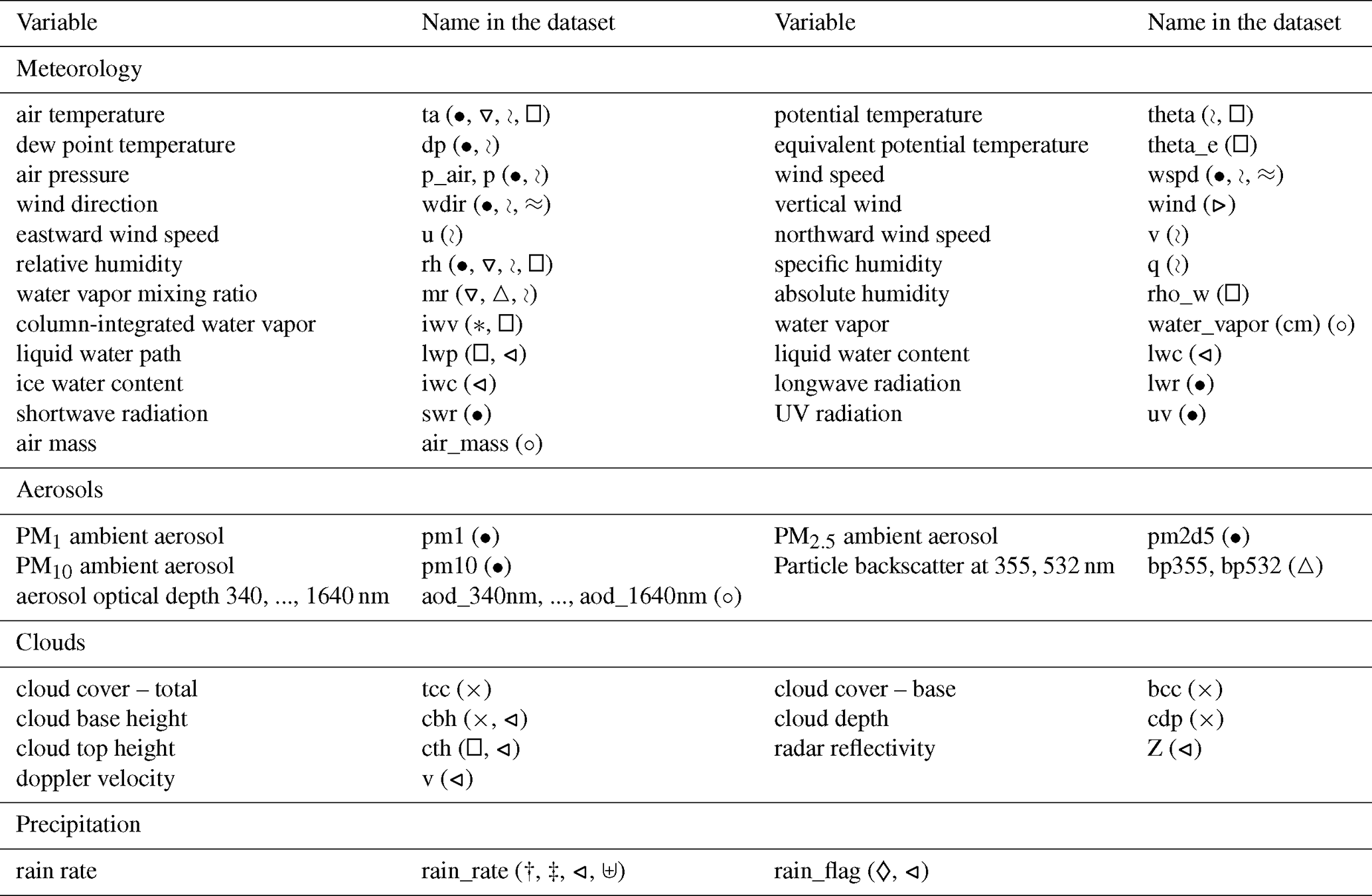
Table 7 The names of the measured oceanic variables, and their respective nomenclature in the data set. The symbol or symbols next to the name in the data set and between parentheses indicate in which data set is used. The symbols are according to Table 1.

4 Insights from instrumentation

As described above, BOWTIE included multiple instruments that measured similar variables. This redundancy was intentional, to allow for identifying and mitigating systematic errors, provide backups in case of instrument failure, and ensure the robustness of results. Here, we explore complementary measurements of four quantities – column-integrated water vapor, rain detection, surface current, and sea surface temperature – as an example of how different instruments can be combined to assess data reliability.

4.1 Integrated Water Vapor

IWV is an important variable for characterizing the local environment, as it is intimately coupled to tropical rainfall (Bretherton et al., 2004). It is, therefore, a variable of special emphasis in this campaign for analysis of the convective environment. IWV is derived from four different instruments: radiosondes, microwave radiometers, microtops, and GNSS (Fig. 5).

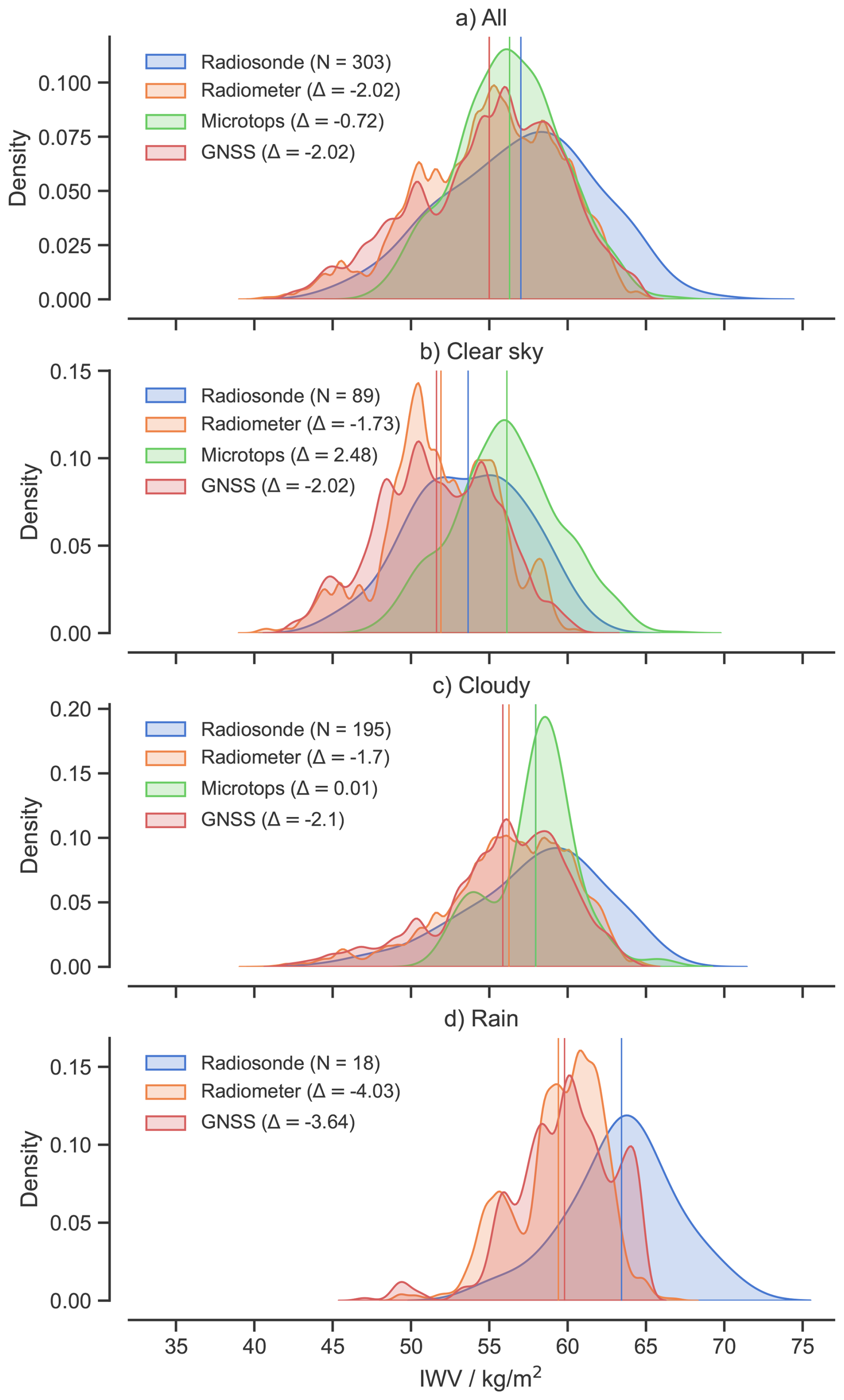
Figure 5 Kernel density estimate (KDE) plots of IWV estimated from multiple datasets (see legend), with means indicated by vertical lines and deviations (Δ) from that of the radiosondes indicated in the legend. The complete dataset (a) is separated into clear-sky (b), cloudy (c), and rain conditions (d). The sample size for the radiosondes (N) in each category is indicated in the legends.

Multiple approaches were tested for calculating integrated water vapor from radiosondes (not shown), using the following equation

$$\begin{array}{}\text{(1)}& \text{IWV}=\underset{z_{\mathrm{base}}}{\overset{z_t}{\int }}q\mathit{\rho }\mathrm{d}z,\end{array}$$

where q is specific humidity (mass of water vapor per mass of total air) and ρ is air density, calculated accounting for moisture effects consistent with Schulz and Stevens (2018). While z_base is generally taken to be the lowest available measurement, for this comparison we take z_base=30 m to match the elevation of the radiometer. The change from 0–30 m amounts to a mean decrease of 0.37 kg m⁻² for the radiosonde dataset, bringing it closer to that of the radiometer.

For all conditions (Fig. 5a), the instruments with the most regular sampling – radiosondes, radiometers, and GNSS – differ by approximately 2 kg m⁻², with radiosondes being moister. IWV retrieved from GNSS and microwave radiometer is similar. Microtops is closer to radiosondes, differing by only −0.72 kg m⁻², but this measurement was taken irregularly throughout the campaign. This irregularity could lead to biased sampling.

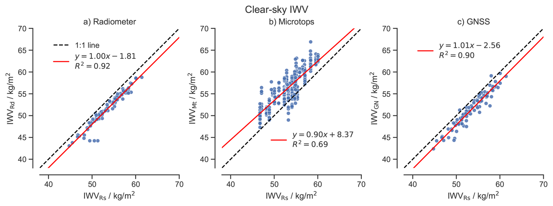
Figure 6 Radiosonde IWV (IWV_Rd; kg m⁻²) plotted against IWV from the (a) radiometer (IWV_Ra), (b) microtops (IWV_Mt), and (c) GNSS (IWV_GN) in clear-sky conditions, with measurements temporally matched between datasets using a nearest-neighbor approach. One-to-one and linear regression lines are depicted.

The additional panels of Fig. 5 separate the comparison into clear-sky, cloudy, and raining conditions, identified through a combination of rain gauge, ceilometer, and cloud radar data. Measurements using microtops were pointing directly at the sun when the line of sight between the microtops and the sun was free of clouds. This means that, under partly cloudy conditions, measurements were taken only if no clouds were in the line of sight to the sun. This explains microtop measurements in the cloudy category. Figure 5b–d depict IWV increase from clear-sky to raining conditions, as expected, with mean IWV from radiosondes increasing from about 54–64 kg m⁻². Values of IWV from GNSS and microwave radiometer are about 2 kg m⁻² lower than radiosonde-derived values in clear-sky and cloudy conditions. IWV derived from microtops is substantially greater than radiosondes in clear-sky conditions (Δ≈2.5 kg m⁻²), but the discrepancy is near 0 kg m⁻² in cloudy conditions. Thus, microtops is the instrument retrieving greater values of IWV compared to the other three sensors in clear-sky conditions.

Discrepancies in IVW between radiosonde measurements and microtops are different between clear-sky and cloudy conditions, which is not the case between radiosondes and both the GNSS and microwave radiometer. Because of this discrepancy between microtops and radiosondes, we assess the relationship between radiosondes and the other measurements in clear-sky conditions in Fig. 6. With clear-sky conditions isolated, the discrepancy between radiosondes and the radiometer is found to be constant with IWV, with the slope of the best-fit line being 1. Moreover, the discrepancies between the integrated water vapor measured by the radiosondes and the microwave radar are independent of daytime and nighttime (not shown). This indicates no dry bias in radiosondes during daytime.

IWV derived from microtops is substantially greater than that of radiosondes at low values of IWV, with the discrepancy decreasing at a rate of 0.1 kg m⁻² per unit IWV. Consistent with Fig. 5, GNSS exhibits a very consistent discrepancy from radiosondes that is nearly invariant with IWV.

It remains unclear what explains the discrepancy of ∼ 2 kg m⁻² between radiosondes and the other measurements. The RS41 radiosondes used here are considered a highly accurate benchmark in situ measurement to which other instruments are compared and often calibrated (Sun et al., 2021). Data users should bear these discrepancies in mind, and future work should investigate their possible causes.

4.2 Rain detection

The exact quantification of the occurrence and amount of surface rain is very difficult, especially on a moving platform like a ship. Spatial variability, especially on small scales, as well as the method to quantify precipitation, can lead to different results in measured rain amount (Yuter and Parker, 2001). These factors could also impact the timing at which instruments effectively measure precipitation. The latter could be translated into the following question: How different is the occurrence of rain detected among the instruments during BOWTIE? This has implications for whether it is enough to use the rain flag from a single instrument or not. Here, rain observations from the micro rain radar, the cloud radar, two disdrometers, and the rain gauge station are compared for the period between 18 August, 06:00 UTC, and 21 September, 23:59 UTC. This analysis aims to indicate to the reader whether it is appropriate to choose one or more instruments when flagging rain.

For the rain gauge and the two disdrometers, which have a time step of 1 min, the time series of rain rate is used to construct the rain detection flag. Three different time windows are chosen: 1, 5, and 10 min. In each window, the rain detection flag is 1 when the rain rate is larger than 0 mm h⁻¹ at least once. The rain detection flag is 0 when the rain rate is 0 in the entire window.

One of the variables derived from the micro rain radar (manually) and the cloud radar (within the Cloudnet processing) is a rain detection flag, which is set to 0 for no rain and 1 for rain (see Sect. 3.2.1). The micro rain radar has a temporal resolution of 1 s, whereas the Cloudnet-processed cloud radar data has a temporal resolution of 30 s. To homogenize our analysis to the rain gauge station and the disdrometers, three time windows are used: 1, 5, and 10 min. In each window, the rain detection flag is 1 if rain is detected at least once in the window; otherwise, the rain detection flag is 0.

Based on the 1, 5, and 10 min rain detection time series, the total number of times that five, four, three, and two instruments detected rain simultaneously is computed. Likewise, the total number of times that a single instrument detected rain is calculated. The frequency is shown in Fig. 7. The total number of times that rain was detected (referred to as events) during 1, 5, and 10 min periods is 6681, 1641, and 939, respectively. The percentage of events detected by a different number of instruments is similar regardless of the time step used. Nearly 33 % of the events were detected simultaneously by the five different instruments. About 18 % of the time, rain was observed by 4 instruments, while around 13 % of the time, it was observed by 3 or 2 instruments only. The percentage of events detected by only one instrument is 23 %.

Events detected by only one instrument are not homogeneously partitioned among all the instruments, as shown in Fig. 7d–f. In this category, the micro rain radar is the instrument with the highest detection rate of rain, independent of the time resolution. Considering the 1 min time step, the micro rain radar accounts for 80 % of the events in which only one instrument detected rain, followed by the rain gauge, with 16 %. The two disdrometers and the cloud radar are the only instruments to detect rain in less than 3 % of the one-instrument-only events. From the two disdrometers, DSD_METEOR1, whose sampling path is in a bow-stern direction, did not detect rain alone (0 %), while DSD_ METEOR2, which has a port-starboard direction sampling path, accounted for 2.5 % of the events. For the 5 and 10 min time steps, 70 % of the rain events are only detected by the micro rain radar, and 27 % are only detected by the rain gauge.

The differences in the detection of rain across the instruments can be explained by several factors. While rain gauges and disdrometers measure rain in situ near the surface at their respective installation point, the micro rain radar and the cloud radar are remote-sensing instruments from which rain detection is derived at an altitude of ∼ 160 m above the ship. This difference in the height of the precipitation measurement, combined with the facts that (i) rainfall can partially or fully evaporate in dry surface layers (Kalesse-Los et al., 2023) and (ii) ship steaming speed and horizontal wind velocity can induce turbulence effects around the in-situ rain sensors, can lead to notable differences in the rain detections. Full evaporation of precipitation in the lowest 160 m can occur during light rain/drizzle with small drop sizes and very dry subcloud layers.

The alignment of the disdrometers also seems to play a role in the detection of rain. DSD_METEOR1 recorded less occurrence of rain than DSD_METEOR2 98.4 % of the time. The differences in the frequency of rain detection between the disdrometers can be explained by the ship motion, the turbulence induced by the ship's structure (Yuter and Parker, 2001), and the turbulence induced by the instrument (Friedrich et al., 2013a). Induced turbulence by the ship's structure and instrument is tied to the changing nature of wind speed and direction, and ship motion. The difference in rain rate measured by the two disdrometers is related to the direction of the wind and their orientation with respect to the steaming direction of the vessel rather than the speed (not shown). In this sense, two disdrometers perpendicular to each other with respect to their sampling path are affected differently by rain from different wind directions and can differ in their rain detection measurements, in terms of the occurrence, as shown in this analysis.

The difference in rain detection between the micro rain radar and the cloud radar can be attributed to the similar reflectivity threshold used to state whether rainfall occurred or not. For both instruments, rain occurrence is set to true if the radar reflectivity at ∼ 160 m (fourth radar range gate) is greater than 3.1 dBZ. However, in rain, the radar reflectivity measured by the micro rain radar is greater than that of the cloud radar because for drops larger than about 1.2 mm, the Rayleigh assumption is no longer valid for the higher-frequency cloud radar. Instead, scattering of larger particles occurs in the Mie regime, in which the linear relation between scattering cross section and particle size is not true, leading to reduced reflectivities. Furthermore, the cloud radar suffers from stronger attenuation effects caused by high IWV values, as well as cloud droplets and rain itself, also leading to reduced observed reflectivities. Consequently, the micro rain radar detects rain onset earlier and rain end later. For example, on 21 August, rain onset by the micro rain radar was detected at 23:14 UTC, whereas the cloud radar only started to detect rain at 23:46 UTC (Fig. 8a) when the reflectivity threshold was reached (Fig. 8b). Before that time, the cloud radar observed falling drops in the lowest radar range gates (Fig. 8c), but the reflectivity values were too low to set the rain flag to true. Decreasing the reflectivity threshold value in the cloud radar would thus allow an earlier detection of rain, as indicated by the 0 dBZ reflectivity contour line in (Figure 8b).

Overall, this analysis provides an estimate of the rain detection uncertainty, which can arise due to the differences in each instrument's sensitivity, measurement principles, effective measurement volumes (smaller for in-situ sensors than for radars), and post-processing. The differences in rain amount between instruments installed on ships have been addressed in Yuter and Parker (2001). Dry near-surface layers can also explain differences between rainfall amounts of remote-sensing and in-situ instruments (Kalesse-Los et al., 2023). Our analysis shows that the rain occurrence between the instruments can also differ, even if measurements are averaged for 10 min. Among the instruments, the micro rain radar and the rain gauge are the ones with a higher frequency of rain occurrence on the ship. Thus, using rain flags from only one instrument is not enough for the BOWTIE campaign.

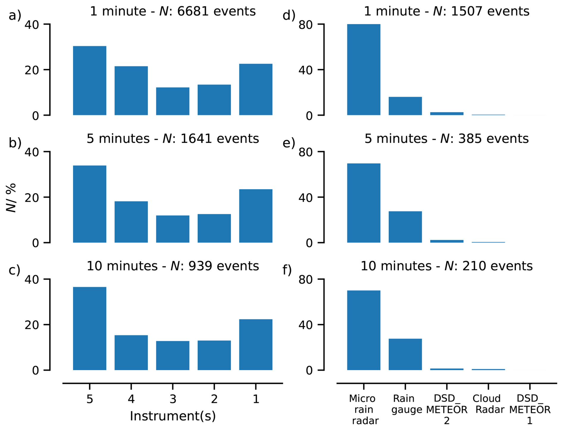
Figure 7 The relative frequency in percentage of times that rain was detected simultaneously by 5, 4, 3, 2, and only 1 instrument using time series of 1 min time step (a), 5 min time step (b), and 10 min time step (c). Relative frequency in percentage of times that rain was detected by only one instrument in a 1 min time step (d), 5 min time step (e), and 10 min time step (f). The instruments are the micro rain radar, the rain gauge station, two disdrometers (DSD_METEOR1 and DSD_METEOR2), and the cloud radar. The absolute number of times N that rain was detected is shown in the title of each panel.

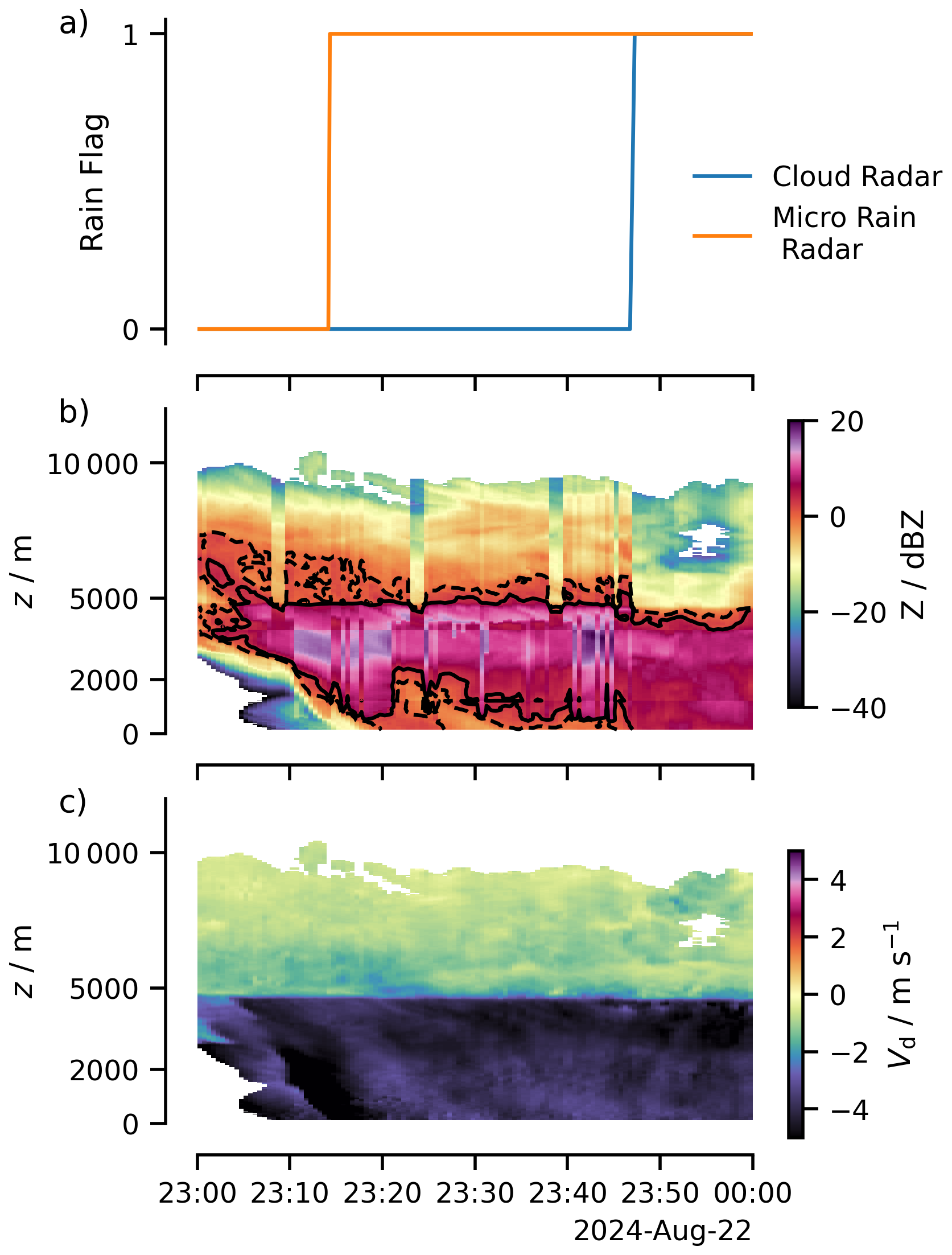
Figure 8 Precipitation event on 21 August 2024. (a) Rain detection flag for the micro rain radar (orange) and the cloud radar (blue). 0 refers to no rain detected, and 1 refers to rain detected. (b) Radar reflectivity time-height plot of the cloud radar (color shading). The 0 and 3.1 dBZ lines are shown in black dashed and solid lines, respectively. (c) Mean Doppler Velocity time-height plot of the cloud radar. Melting layer height is indicated by a strong increase in Mean Doppler Velocity at around 5000 m.

4.3 Ocean surface currents

During the BOWTIE experiment, ocean surface currents were measured using two systems: vessel-mounted ADCPs (vmADCPs) and an X-band marine radar (see Sect. 3.2.3). VmADCPs are subject to inherent limitations when resolving near-surface currents, as their installation below the ocean surface, combined with the instrument blanking distance, results in blind zones in the upper water column. These layers are further degraded by ship-induced bubble clouds and residual inaccuracies in motion compensation. Consequently, the shallowest reliable current estimate obtained from the 75 kHz vmADCP corresponds to a depth-averaged measurement spanning approximately 13 to 21 m.

Current measurements derived from X-band marine radar are inferred by analyzing the evolution of the wave field in the frequency–wavenumber domain and identifying the most probable current velocities consistent with the wave dispersion relation. The retrieved current, therefore, represents a depth-averaged flow weighted by the wave-induced orbital motion, rather than a direct measurement at a fixed depth. A key question associated with this approach is the effective sensing depth of the retrieved currents. According to Lund et al. (2015), this depth corresponds to approximately 7.8 % of the dominant wavelength for a linear vertical current profile, and 4.4 % of the wavelength for a logarithmic current profile. Assuming a logarithmic current profile and a typical dominant wavelength of 80 m, the effective depth of the retrieved current is approximately 3.5 m.

A direct comparison between the two sensors is inherently challenging because vmADCP measurements are collected directly at the vessel location, whereas radar observations cannot be acquired at the same position and time due to vessel-induced imaging disturbances. As a result, radar-derived currents at this location are available only before or after the vessel’s presence. To address this limitation, a workaround strategy is employed in which radar and ADCP measurements are aggregated into time windows sufficiently long to ensure that the vessel fully traverses the target location. In this study, the data are grouped into 15 min intervals, within which all available measurements are temporally averaged. The averaged radar and vmADCP currents are then directly compared.

Figure 9 illustrates the resulting comparison between both instruments. A systematic trend is observed, with radar-derived surface currents (representative of approximately 3.5 m depth) exceeding vmADCP currents measured at 17 m depth. This result is consistent with vertical shear induced by wind drag in the uppermost ocean layer. The greater bias metric is observed in the zonal currents than in the meridional currents. The root mean square error is also higher in the zonal currents than in the meridional direction. These results indicate a stronger impact of the wind drag in the zonal component than in the meridional one at 17 m depth. This is observed when classifying the data with respect to the ship velocity (not shown). The Pearson correlation indicates that the zonal and meridional currents between the first 3 m depth and 17 m depth show a similar 15 m variability. In the zonal direction, 88 % of the variability of the ADCP measurements can be explained with X-band measurements. In the meridional direction, the explained variability is 81 %.

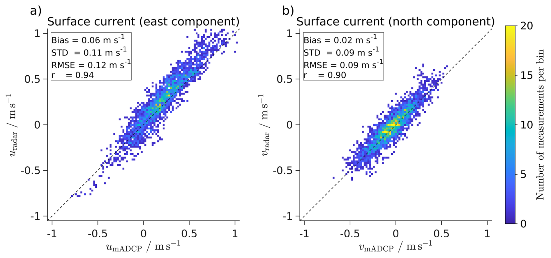
Figure 9 Comparison of quality-controlled vmADCP and X-band radar-derived ocean surface currents. VmADCP measurements at 17 m depth (x-axis) are compared with radar-derived currents representative of approximately 3.5 m depth (y-axis). (a) Eastward component. (b) Northward component. The color scale represents the number of observations per bin. The dashed black line marks the one-to-one correspondence, and the inset rectangles report bias, standard deviation, RMSE, and Pearson correlation coefficient. A quality-control criterion is applied to the vmADCP using a quality flag ranging from 0 to 9. Only measurements classified as good data (QC = 1) or probably good data (QC = 2) are retained for the analysis. Radar-derived currents are quality-controlled using the signal-to-noise ratio (SNR), where higher values indicate greater confidence. Only radar measurements with SNR > 5 are considered in the comparison.

4.4 Sea surface temperature measurements

The temperature of the sea surface is an important quantity because of its use in the calculation of the exchange of energy and moisture between the ocean surface and the lower troposphere. It is known that measurements of what is referred to as sea surface temperature (SST) can vary with depth (Saunders, 1967; Fairall et al., 1996), reflecting different processes in the first meters of the upper ocean. At the air-sea interface (skin), molecular heat conduction is the principal mechanism of heat transfer. Because it is thin, its heat capacity is low, making the skin tenths of a degree colder than a few centimeters (sub-skin) or even a few meters (bulk) below the skin (Saunders, 1967). Below the skin layer, turbulence efficiently distributes heat, allowing the vertical temperature gradient to be small; however, in the presence of light wind regimes and daytime conditions of net heat input, turbulence decreases, and heat is trapped in the first meters of the upper ocean. If insolation is strong, the temperature stratification is strong, developing a diurnal warm layer (Price et al., 1986; Fairall et al., 1996). This results in warmer temperatures in the sub-skin layer than in both the bulk measurements and the skin layer (Minnett, 2003). It is also possible for the skin layer to be warmer than the bulk measurements. Given this background, the measurements during BOWTIE are analyzed to identify (1) whether BOWTIE measurements are consistent with these expectations, and (2) possible errors in the measurements.

The three products used are from ISAR, the thermosalinograph, and the sea snake, all of which incorporate quality flags (see Sect. 3.2.3). ISAR measures the skin layer temperature (SST_skin), the sea snake measures the sub-skin layer temperature at 5 cm (SST_5 cm), and the thermosalinograph measures the bulk temperature at 5 m (SST_5 m) below the ocean surface. Figure 10a shows the time series of SST_skin, SST_5 cm, and SST_5 m during the BOWTIE campaign. At first glance, there is a good agreement between SST_5 cm and SST_5 m, except in certain periods related to light wind regimes, such as on 26 August (see Sect. 5.1). The skin layer is colder than the sub-skin layer or the bulk measurements most of the time. While this is expected, SST_skin can be more than 1 K colder than the sub-skin layer or the bulk measurements, which is much colder than previous observations (e.g., Robinson et al., 1984; Minnett, 2003; Fairall et al., 2026).

To further analyze how much colder the ISAR-measured skin layer is according to ISAR, we compute the difference between the skin layer and bulk measurements (SST_skin − SST_5 cm) at night (between 22:00 and 05:00 local time), as well as the difference between the sub-skin layer and the bulk measurements (SST_5 cm − SST_5 m). These hours were selected to avoid any influence of diurnal warm layers. Moreover, only time steps when all three instruments have measurements are taken into account. Figure 10b depicts the typical temperature structure of the upper ocean. As expected, the difference between the sub-skin layer and bulk measurements is small, with a mean difference of 0.008 K and a standard deviation of 0.09 K. The skin layer is tenths of a degree colder than the sub-skin layer most of the time, with a mean difference of −0.6 K and a standard deviation of 0.5 K. The large standard deviation in the difference between the skin and the sub-skin layer (cold layer) is due to measurements in which the skin layer was colder than the sub-skin layer by 1 K. Restricting to values of ΔSST${}_{\text{skin – 5\hspace{0.17em}cm}}>-\mathrm{1}$ K gives a standard deviation of 0.17 K and a mean of −0.43 K, which is in the range of expected values. Possible factors for a much colder skin layer (ΔSST${}_{\text{skin – 5\hspace{0.17em}cm}}<-\mathrm{1}$ K) than expected, such as changes in downwelling longwave radiation or in factors controlling surface heat fluxes (wind speed, relative humidity, and temperature), are not different from other nights where ΔSST${}_{\text{skin – 5\hspace{0.17em}cm}}\ge -\mathrm{1}$ K. The development of the too cold layer (ΔSST${}_{\text{skin – 5\hspace{0.17em}cm}}<-\mathrm{1}$ K) is observed for 4.7 % of the total measurements during night hours. Figure 10b shows that the occurrence of too cold skin layers is not explained by wind speed. While rain can cool the skin layer (Witte et al., 2023) or introduce noise in the measurements, there were no rain events over the ship when ΔSST${}_{\text{skin – 5\hspace{0.17em}cm}}<-\mathrm{1}$ K. To the knowledge of the authors, no previous campaigns have shown such a cold difference in ΔSST_{skin – 5 cm}. Therefore, we do not currently have an explanation for why the ISAR skin temperature measurements are sometimes unexpectedly cold.

To analyze the development of diurnal warm layers and how they are observed in BOWTIE, a similar analysis is conducted for daytime hours, from 10:00 to 18:00 local time (Fig. 10c). The difference between the sub-skin temperature and the bulk temperature (shading in Fig. 10c) is notably larger under conditions of light wind speed. The maximum difference was 2.43 K, on 26 August during light wind conditions. At the time of the maximum ΔSST_{5 cm – 5 m}, the skin layer was 0.44 K colder than the sub-skin layer. This means that the skin layer was 2 K warmer than the bulk measurements. The picture of SST_5 m< SST_skin< SST_5 cm is typical of diurnal warm layers. However, Figure 10c also shows that in certain periods, not always, the skin was warmer than the sub-skin layer (ΔSST_{skin – 5 cm}> 0 K). The maximum ΔSST_{skin – 5 m} ( 2.34 K ) on 26 August coincides with a skin layer 0.81 K warmer than the sub-skin layer. ΔSST_{skin – 5 cm}> 0 K has been observed in the mid-latitudes and is called a “warm skin event” (Jia and Minnett, 2023). The fact that the skin layer is warmer than the sub-skin layer indicates an input of energy into the ocean, and is associated with a reduction in surface heat fluxes or an increase in downwelling longwave radiation. The former is the most probable due to the light winds. Nevertheless, ΔSST_{skin – 5 cm} can be smaller than −1 K during the daytime (a too cold skin layer), and this accounts for 4 % of the measurements. Only one measurement of the too cold skin layers during daytime is related to a rainfall event; we lack an explanation for the other instances of these cold ISAR skin temperature measurements.

Overall, BOWTIE's measurements of near-surface ocean temperatures at different depths are consistent with expectations regarding a cold skin layer and the development of diurnal warm layers under light wind conditions. However, there are instances of too cold skin layers from the ISAR measurements (ΔSST${}_{\text{skin – 5\hspace{0.17em}cm}}<-\mathrm{1}$ K). Including all measurements, too cold layers account for 15 % of the measurements. Until a physical explanation is provided for such too cold skin-layers events, it is recommended to avoid the use of those events for scientific analysis.

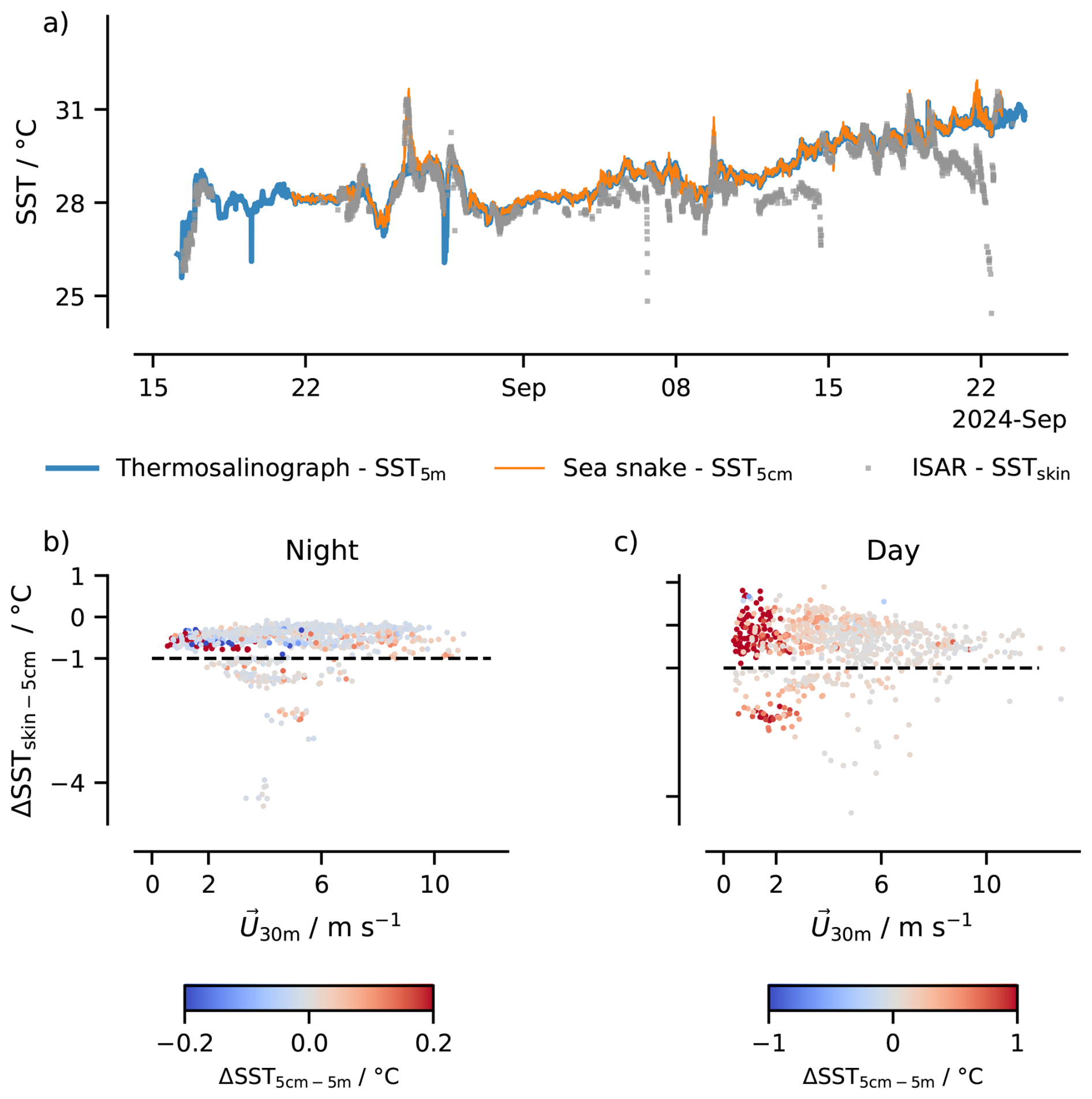
Figure 10 Ocean temperature measurements at the skin (SST_skin; ISAR), 5 cm (SST_5 cm; sea snake) and 5 m (SST_5 m; thermosalinograph) during BOWTIE. (a) Time series for the entire campaign of SST_skin (thick solid blue line), SST_5 m (Solid orange line), and SST_skin (gray thick dots). (b) Scatter plot of the difference between SST_skin and SST_5 cm (ΔSST_{skin – 5 m}) and wind speed measured at 30 m above water line (U_30 m) colored by ΔSST_{5 cm–5 m}. The analysis is done for nighttime hours, from 22:00 to 05:00 local hours. The dashed black line indicates a ΔSST_{skin – 5 m} of −1 K. (c) Same as (b) but for daytime hours, from 10:00 to 18:00 local hours. In (b), (c) only time steps in which the three instruments have valid measurements are taken into account. For ISAR, the quality levels chosen are “acceptable_quality” and “best_quality”, attributes of the “quality_level” class inside the ISAR dataset. The thermosalinograph and the sea snake share a similar class for the flag of quality level, “TEMP_QC”. Only measurements with a flag of “good_data” and “probably_good_data” are selected.

5 Case studies of the inner ITCZ

In this section, we present two scientific case studies that exemplify the use of the BOWTIE dataset and address key scientific motivations of the campaign. The first case study focuses on light-wind conditions, while the second examines a strong-wind regime. Both cases highlight the wealth of observations enabling the study of these atmospheric phenomena regarding processes in the atmospheric boundary layer, including near-surface variables in the atmosphere and SST in the case of the doldrums. While not studied here, the BOWTIE data set also allows the analysis of such atmospheric phenomena and their interaction with the upper ocean.

5.1 Doldrums

One atmospheric mesoscale phenomenon targeted by BOWTIE is the doldrums, characterized by weak surface winds. Their role in shaping local convection within the ITCZ remains an open question (Windmiller, 2024). Global storm-resolving simulations further suggest that the doldrums can influence tropical climate more broadly (Segura et al., 2025). The impact of doldrums on local convection and the large-scale circulation is challenging to determine, because of the limited information on the scales controlling the air-sea energy and momentum transfer when winds slacken. This calls for a comprehensive characterization of the structure of doldrums regarding their energetics and momentum, i.e., the evolution of the atmospheric boundary layer and upper ocean. Two questions arise here: Were doldrums observed during BOWTIE? And what are the thermodynamic and dynamic structures of doldrums?

Using the DShip data, we identified instances in which the 10 min running mean of the wind speed measured at 30 m was below 3 m s⁻¹ continuously for at least 10 min. There were 90 such instances of these light wind events. Prior studies have used various definitions of doldrums, which typically require the light wind events to be present for a sufficiently long period of time (hours) to indicate a persistent event that is also likely widespread spatially. During BOWTIE, we observed 28 light wind events that lasted for at least an hour, 18 for at least 2 h, 10 for at least 3 h, 8 for at least 4 h, 6 for at least 5 h, and 2 that lasted at least 6 h. Thus, taking one hour as the threshold, 28 doldrums were observed. The longest-duration doldrum event was observed from 26 August at 11:10 UTC to 27 August at 02:25 UTC, having a duration of 15 h and 15 min. This is the event whose evolution is examined in Fig. 11.

Figure 11 shows that leading up to and during the doldrum event on 26 August, the sky conditions were mostly clear until late afternoon, as the ceilometer detected cloud bases only for a few short periods of time. The weak wind and mostly clear-sky conditions resulted in a diurnal warm layer, in which the sub-skin ocean temperature measured by the sea snake was up to 2.34 K warmer than the bulk temperature measured by the thermosalinograph. This was the strongest diurnal warm layer measured during the campaign, as discussed above in Sect. 4.4.

Measurements using radiosondes make it possible to characterize the vertical structure of the atmosphere when doldrums occur. Figure 12 shows the temporal evolution of wind speed, specific humidity, and potential temperature of the first kilometer measured by the radiosondes from 10:46 UTC (08:00 LT) to 22:50 UTC (20:50 LT) on 26 August. Light winds occurred throughout the first kilometer of the atmosphere, and it is sustained throughout the event. This means that doldrums are not just wind events occurring at the surface but also in the whole boundary layer. The homogeneous structure of winds along the boundary layer is also observed in the structure of humidity and temperature. This means that despite the fact that winds are light, at least this doldrums event shows a homogeneous structure of the dynamics and thermodynamics in the boundary layer. Thus, one could ask which type of scales are driving this homogenization of the structure of the boundary layer and what the implications are for the surface heat fluxes during doldrums.

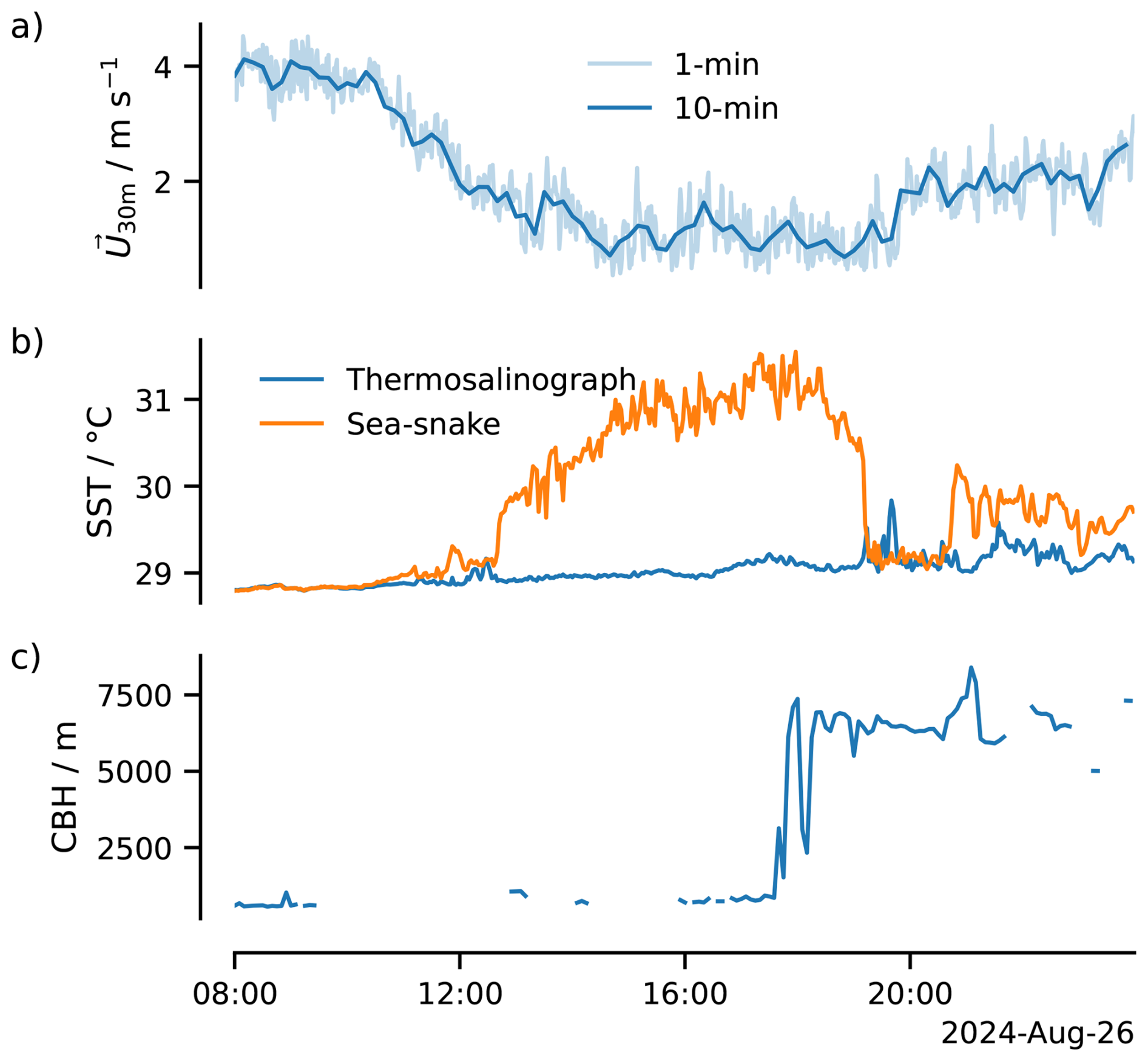
Figure 11 Doldrums event on 26 August 2024: Time series of (a) wind speed (U_30 m) with 1 min time step (light blue) and 10 min mean (dark blue), (b) sea surface temperature (SST) from the thermosalinograph (blue line) and sea snake (orange line), and (c) cloud base height from ceilometer (CBH; blue line). Wind speed and SST from the thermosalinograph are part of the DShip data.

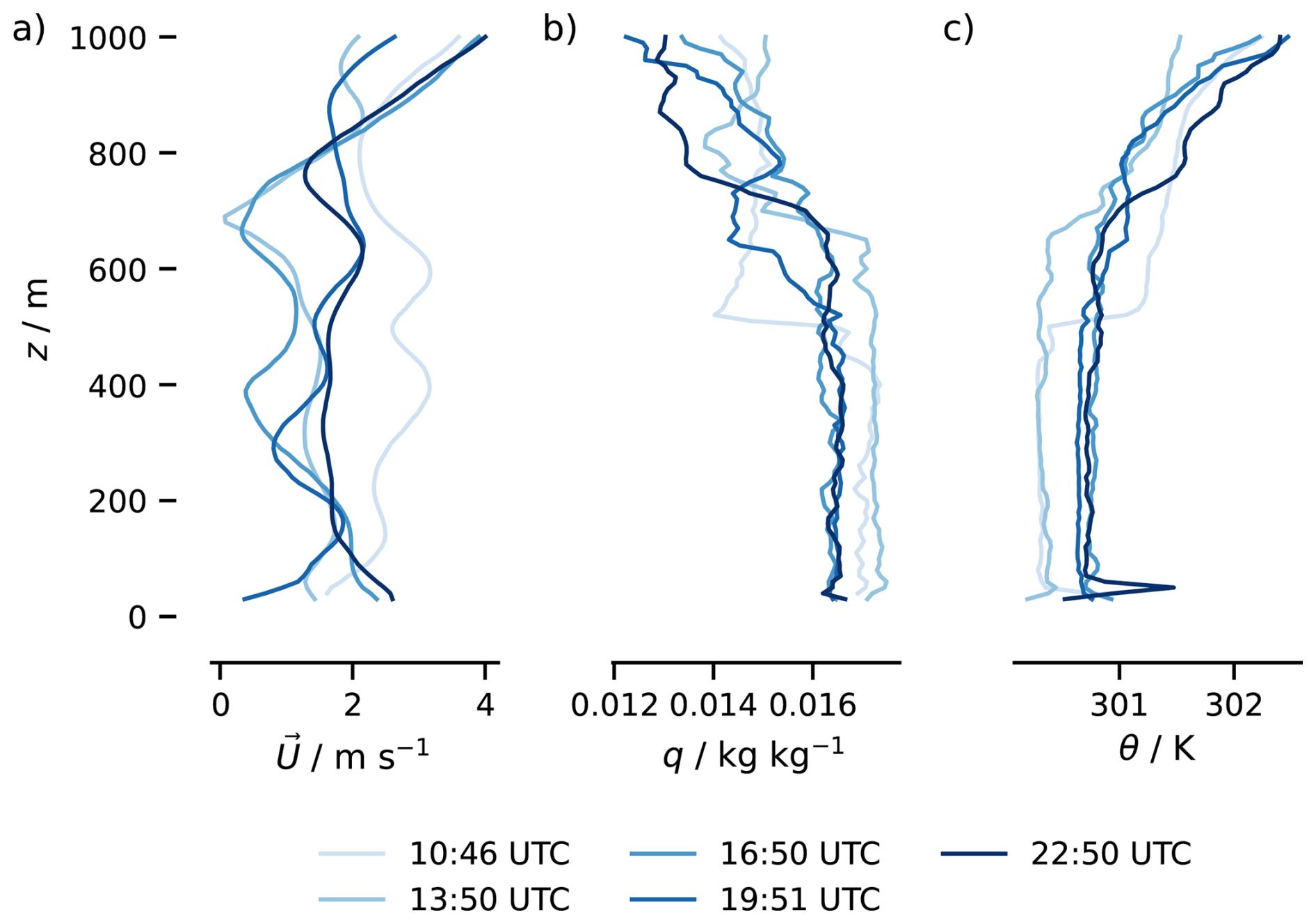
Figure 12 Doldrums event on 26 August 2024: temporal evolution of (a) wind speed (U), (b) specific humidity (q), and (c) potential temperature (θ) from radiosondes. Only data above 30 m height are shown. Colors indicate the time in UTC when the radiosonde was launched.

5.2 Precipitation and gust front

Convective precipitation results from interactions across scales, from cloud microphysics to the large-scale circulation, coupling thermodynamic, dynamic, and radiative processes. Characterizing convective systems therefore requires observations of their energetics and momentum, a key objective of BOWTIE, PICCOLO, and STRINQS. During BOWTIE, precipitation exceeding 1 mm was recorded by the rain gauge station on 21 d. On 8 September, ∼ 8 mm of rain was measured. This amount of rain is due to a squall line crossing the ship. A gust front ahead of the squall line was also observed.

On 8 September, around 12:00 UTC, the disdrometer detected precipitation rates greater than 5 mm h⁻¹, indicating the presence of intense precipitation (Fig. 13a). This is confirmed by Sea-Pol, in which the quasi-vertical scan revealed that high precipitation intensities occurred below 5 km altitude (Fig. 13b). The Cloudnet retrieval also indicated substantial liquid water content in the lowest few km (Fig. 13c). Sea-Pol's scanning capabilities provide information on the 3D structure of precipitation (Fig. 14). RHI scans of the squall line indicate that it consisted primarily of congestus (echo tops of 5–7 km), though some deeper convection is found further from the ship (Fig. 14c). Dual-polarimetric measurements reveal microphysical characteristics of the precipitation; for example, higher differential reflectivity (ZDR) values (Fig. 14d) indicate a larger average size of the raindrops. An increase in both reflectivity and ZDR towards the surface indicates collision-coalescence processes. The areas where ZDR is higher, and reflectivity is lower near the surface, are likely due to size sorting, where the bigger drops fall faster than the smaller ones, though faster evaporation of smaller drops could also contribute.

During that precipitation event, the anemometer on the ship measured a sharp increase in wind speed of about 10 m s⁻¹ (Fig. 13d), indicating that this precipitation event was associated with a gust front. This may be caused by evaporation of precipitation before it reaches the surface, cooling the air and leading to a downdraft that spreads horizontally as a gust front when it hits the surface. Following the passage of the leading edge of the gust front and the occurrence of precipitation, the boundary layer cooled significantly, as shown by a drop of 4 K in air temperature measured by the thermometer on the ship (Fig. 13e).

The characterization in this study is only a first step towards a deeper analysis regarding the interaction between cloud particles and radiation, turbulence in the boundary layer, and the impact of convective systems in the air-sea exchange of momentum and energy. This can be done by combining measurements from the Sea-Pol and cloud radars, aerial drones, radiosondes, and radiation measurements on the ship.

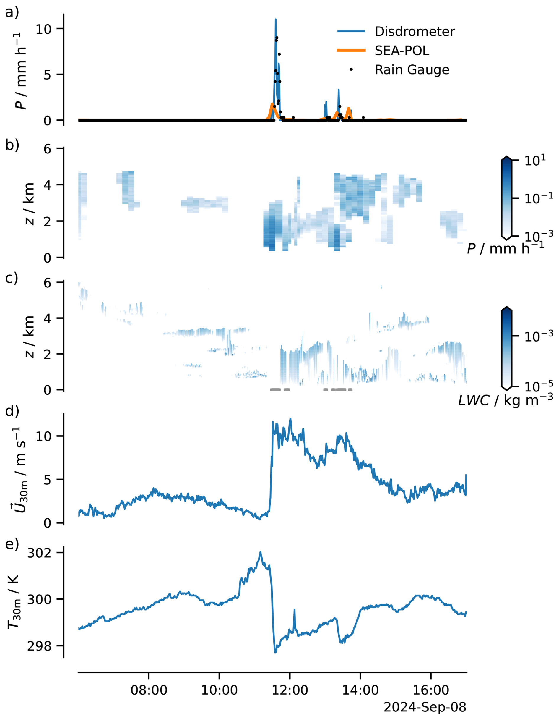
Figure 13 8 September case study. (a) Precipitation intensity (P) from the disdrometer (blue line), rain gauge (black dots), and average within 1 km of the ship from the Sea-Pol low-level scan (orange line). Temporal evolution of (b) the vertical structure of precipitation from the Sea-Pol quasi-vertical profile and (c) the vertical structure of liquid water content (LWC) from the Cloudnet retrieval. The gray dots in the third row indicate when the LWC retrieval is not possible due to rain detection. Time series of (d) wind speed (U_30 m) and (e) temperature (T_30 m) from DShip data.

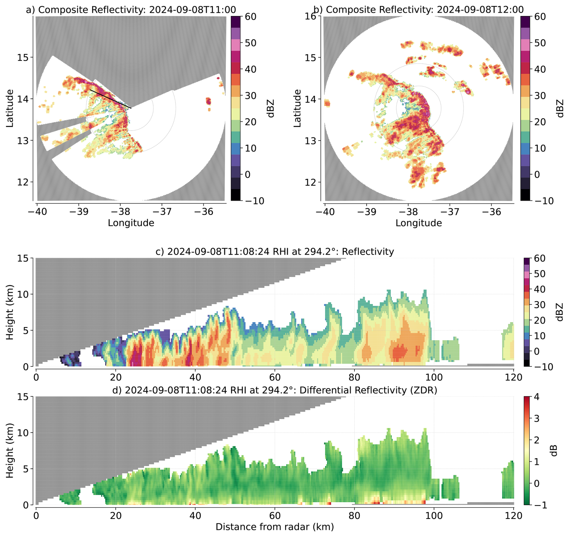
Figure 14 September 8 case study. Spatial distribution of convection (a) before (11:00 UTC; panel a) and (b) after (merged scans from 12:00–12:20 UTC) passage of gust front as depicted by Sea-Pol composite reflectivity. Range rings are shown at 60 and 120 km. Bottom two rows are range-height indicator plots (RHI) showing vertical structure of the squall line at 11:08 UTC, at an azimuth of 294.2° (black line in a) based on reflectivity (c; dBZ) and differential reflectivity (d; dB).

6 Code and data availability

The BOWTIE data is shared using the InterPlanetary File System (IPFS), which allows addressing, routing, and transferring data on the web. Every data set, as well as each version of a given dataset, has a unique identifier in IPFS. This allows tracking of the data that is used. The latest version of the data can always be accessed via https://latest-orcestra--campaign-org.ipns.dweb.link/ (last access: 24 June 2024). A global view of the data can be found in the ORCESTRA data browser (https://browser.orcestra-campaign.org, last access: 24 April 2026). Moreover, BOWTIE's data sets follow the Climate and Forecast (CF) data conventions.

Specific datasets used in this paper are listed in Table 8, along with their IPFS content identifiers.

Segura (2026a)Winkler et al. (2026)Foth (2026a)Colón-Burgos (2026a)Colón-Burgos (2026b)Colón-Burgos (2026c)Dengler (2026a)Bosser (2026)Lind et al. (2026)UoS (2026)Stelzner and Klocke (2026)Klocke et al. (2026a)Klocke et al. (2026b)Bell et al. (2026a)Bell et al. (2026b)Bell et al. (2026c)Bell et al. (2026d)Jansen (2026)Dengler (2026b)Foth (2026b)Foth (2026c)Serikov (2026a)Serikov (2026b)Boedewadt et al. (2026)Nuijens (2026)Serikov (2026c)Serikov (2026d)Serikov (2026e)Foth (2026d)Schlundt (2026)Segura and Wing (2026)Segura (2026b)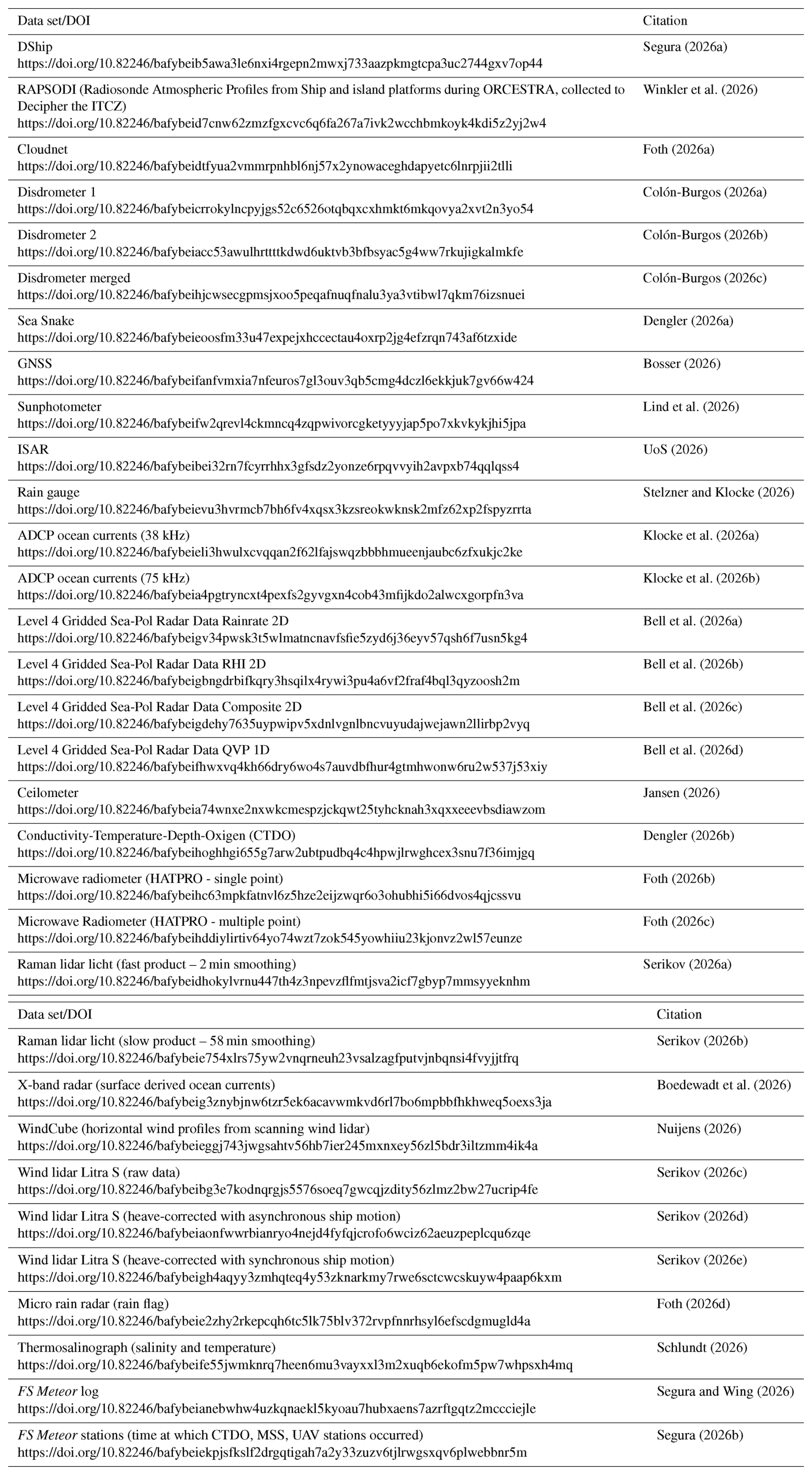

Table 8 Data set: DOI and citation.

The scripts used to produce the figures in this manuscript are available at https://doi.org/10.17617/3.FZYXYF (Segura et al., 2026).

7 Summary

During the Beobachtung von Ozean und Wolken – Das Trans ITCZ Experiment (BOWTIE) campaign, the FS Meteor navigated in the moistest region of the tropical Atlantic for 40 d (Klocke et al., 2026c). FS Meteor departed from the port on Mindelo on 16 August 2024 at 06:00 local time and arrived at the port of Bridgetown in Barbados on 24 September 2024 at 08:00 local time. BOWTIE utilized 29 instruments to measure different properties of the atmosphere, upper ocean, and air-sea interface. Radiosondes were launched every 3 h and provided profiles of the atmosphere up to 30 km. Standard meteorological instruments and thermosalinographs on board provided observations of near-surface variables in the atmosphere and upper ocean with high temporal resolution. Profiles of ocean properties down to 2 km depth were obtained during dedicated CTDO stations, and autonomous oceanographic platforms (gliders, a WireWalker, and a drift buoy) were deployed three times in specific study areas. Instruments using remote sensing techniques provided high temporal resolution profiles of thermodynamic and dynamic properties of the troposphere. Cloud, hydrometeor, and aerosol properties were also sampled. The 2D wind field within the first two km above the surface and 2D currents near the ocean surface were also measured by remote sensing techniques, as well as profiles of ocean currents down to 1.6 km depth. The close collaboration with the PICCOLO campaign permitted measurements of precipitation and hydrometeor properties not only over FS Meteor but within the surrounding area, as far away as 245 km from the ship, by using the Sea-Pol radar. Aerial drones deployed by the STRINQS campaign in dedicated stations mapped profiles of the first 1.5 km of the atmosphere. Most of the data is available in a common repository (https://latest-orcestra--campaign-org.ipns.dweb.link/, last access: 24 April 2026). In this manuscript, only a small fraction of the data has been used in case studies and example analyses. A global view of the data can be found in the ORCESTRA data browser (https://browser.orcestra-campaign.org/, last access: 24 June 2024).

The large number of instruments in BOWTIE and the fact that some of the instruments measured similar or related variables allow us to characterize uncertainties in the measurements. Four examples were selected: (1) column-integrated water vapor, (2) rain detection, (3) ocean surface currents, and (4) sea surface temperature measurements. The comparison of IWV shows that the four relevant instruments – radiosondes, microwave radiometer, microtops, and the GNSS – differ in their measurements by up to 2 kg m⁻². The difference varies depending on the environment (clear-sky, cloudy, and rainy), as environmental conditions affect the accuracy of the instruments using remote sensing techniques. The rain detection analysis indicates that the micro rain radar tends to detect rain more frequently than surface-based instruments for rainfall measurement (rain gauge station and disdrometers). This could be related to possible rain evaporation, strong winds, and ship movements, which could reduce the detection of rain in the rain gauge station and disdrometers. Post-processing procedures can also contribute to differences between remote sensing instruments.

The difference in the ocean current measured by the X-band radar (near-surface) and the ADCP (17 m depth) agrees with expectations. The X-band radar measured stronger currents than the ADCP, and it is independent of the velocity of the ship. It is observed that the difference in the zonal component of the current between X-band and the ADCP is bigger than in the meridional component.

The measurements of ocean temperature at different depths, skin (ISAR), sub-skin (5 cm depth; sea snake), and bulk 5 m depth (thermosalinograph), show the expected cold skin and the development of diurnal warm layers. The latter occurs during light wind regimes. However, there are times when the skin layer is unexpectedly colder than the sub-skin layer by more than 1 K. At the moment, we lack a physical explanation for this behavior, and it is recommended to avoid the use of skin temperature data in events when the skin layer is 1 K colder than the sub-skin layer.

To illustrate the different wind/convection/sea surface temperature regimes that can be encountered within the ITCZ, two case studies are shown: a doldrum event and a precipitation event associated with a gust front. These case studies provide an example of how multiple instruments from BOWTIE can be leveraged to provide a comprehensive characterization of such events. This manuscript serves as a reference for the data collected in BOWTIE and documents the suite of instruments and measured variables. The extensive measurements of the atmosphere, ocean, and air-sea interface across different environments may be leveraged by future studies to investigate questions about atmospheric convection and its interaction with the upper ocean.