A new global dataset of photosynthesis parameters

Photosynthesis-irradiance and photosynthesis-depth experiments are two standard ways of experimentally quantifying primary production. These measurements have historically formed the backbone for the formulation of mathematical models of primary production and to this day remain an invaluable resource for model development and refinement. From such experiments information on photosynthesis parameters can be extracted, which allows for the quantification of the photosynthesis light dependence, essential in the calculation of primary production. To this day, such experiments remain the primary source of photosynthesis parameters, making such data invaluable for primary production modelling. In the literature, there have been several efforts to form global datasets of photosynthesis parameters, collected at various sites across the world oceans and seas. Here, we use a publicly available global dataset of in situ primary production profiles and construct a new database of photosynthesis parameters. We use an inverse modelling approach that is described in great details, along with the data requirements. For a forward model, we employ a fully solvable analytical model of the production profile, and we use the inverse model to compare it with the measured production profile, while constraining it with measured daily watercolumn production. Using this approach, we successfully recovered 3776 photosynthesis-irradiance parameters from the global oceans, which enabled a model versus data comparison for watercolumn production. The spatio-temporal distribution of the new dataset is presented and compared to existing datasets. Finally, the new photosynthesis parameters dataset is provided publicly, along with metadata needed for the implementation in primary production models. The dataset can be accessed via the Zenodo repository at https://doi.org/10.5281/zenodo.17973417 (Kovač et al., 2025).

1 Introduction

Estimation of global marine primary production is an ongoing pursuit of biophysical oceanography (Brewin et al., 2023) and over time a number of models and algorithms have been developed to tackle this problem (Platt and Sathyendranath, 1988; Balch et al., 1992; Antoine et al., 1996; Campbell et al., 2002; Buitenhuis et al., 2013). Modern global state of the art models of marine primary production require four essential sources of information as a minimum: surface photosynthetically active radiation, attenuation coefficients for downwelling radiance, chlorophyll a concentration and photosynthesis parameters (Kulk et al., 2020, 2021; Westberry et al., 2023). Photosynthetically active radiation is readily available as data products on a global scale, or is easily measurable in situ via radiometers. The same would hold for the attenuation coefficient. Depending on the complexity of the models, namely being spectrally resolved or not and on whether the model admits vertical structure in phytoplankton or not (Sathyendranath and Platt, 1989a; Kyewalyanga et al., 1992), data requirements on surface photosynthetically active radiation and attenuation coefficients vary significantly (Platt et al., 2017). Global scale chlorophyll a concentration for the surface ocean is typically estimated by using remotely sensed radiance data, since the time of the seminal paper by Gordon et al. (1983), whereas locally it can be estimated by a variety of observational methods. The final requirements for model implementation are values of photosynthesis parameters, information on which is only available, to this date, via direct measurements of the photosynthesis irradiance curve (Platt and Jassby, 1976), or via inverse modelling based on measured production profiles (Kovač et al., 2017b). Estimation of these parameters via remote sensing still eludes us (but see Topliss and Platt, 1986) and that is why such datasets (Bouman et al., 2018; Kulk et al., 2020, 2021) are an invaluable resource for primary production models. They also help constrain the magnitude of global primary production (Richardson et al., 2016), an important flux in the global carbon budget (Friedlingstein et al., 2025).

In all classes of models, surface irradiance is used as the energy source to drive photosynthesis (Platt and Sathyendranath, 1993; Behrenfeld and Falkowski, 1997b). A light penetration model is used to calculate the underwater light field, in combination with a model for the prescription of the chlorophyll a profile (Platt and Sathyendranath, 1991). Depending on the complexity of the model, the effect of chlorophyll a on the underwater light field may be included in the model (Sathyendranath and Platt, 1989b). However, knowing the chlorophyll a concentration at a given depth, along with the available light, is not enough to calculate the carbon uptake through photosynthesis. The final step is achieved by using photosynthesis-irradiance functions (Platt et al., 1977; Jones et al., 2014), which themselves link chlorophyll a, a state variable, with primary production, a flux, for a given irradiance level (Amirian et al., 2025). By integrating the flux of carbon through photosynthesis over time, typically one day, and over depth, the models arrive at an estimate of primary production per unit ocean surface (Platt et al., 1991). By subsequently integrating over the ocean surface the models arrive at a global estimate of primary production, and further integration over the course of one year yields an annual estimate of primary production (Longhurst et al., 1995; Buitenhuis et al., 2013).

To make the models precise, information on the rate of primary production as a function of light is essential. This is provided by the photosynthesis-irradiance functions, the exact value of which is determined by the values of photosynthesis parameters (Gallegos and Platt, 1981). Direct estimation of photosynthesis parameters is based on costly and scarce field measurements of carbon assimilation by phytoplankton in labelled carbon experiments carried out in vitro, under controlled light conditions (Platt and Jassby, 1976; Bouman et al., 2018). A relatively novel method applies inverse modelling techniques to data from in situ incubations under natural light conditions (Kovač et al., 2016a). The in situ experiments are typically even more expensive and time consuming than direct photosynthesis-irradiance experiments, and the inverse modelling technique serves to extract additional information from them, and to fill gaps in the direct measurements of photosynthesis-irradiance experiments.

The photosynthesis-irradiance experiments provide information on the rate of carbon assimilation as a function of irradiance, and parameter estimation is carried out by first selecting a photosynthesis irradiance function, followed by fitting it to the data (Jassby and Platt, 1976). The results yield best estimates of photosynthesis parameters. The controlled nature of the experiments, and the availability of a large parameter dataset was highly valuable, in that it provided the backbone for the formulation of primary production models based on first principles (Platt et al., 1988, 1990). The latest published archive of photosynthesis parameters estimated in such a way holds 5711 estimated values of photosynthesis parameters from around the global ocean (Bouman et al., 2018). These parameters (or earlier subsets of the data) are routinely used in global models of primary production (Longhurst et al., 1995; Kulk et al., 2020, 2021).

The other set of measurements routinely performed at sea is the in situ implementation of the carbon assimilation method (Strickland and Parsons, 1972; Peterson, 1980; Behrenfeld and Falkowski, 1997a). These measurements provide information on the vertical structure of primary production (often reported as daily rates), the so called production profile. Measured production profiles have not been used routinely to derive photosynthesis parameters, until suitable methods emerged (Kovač et al., 2016a). These methods use inverse modelling to find the optimal values of photosynthesis parameters based on measured production profiles and have been successfully tested at two time series stations: Hawaii Ocean Time Series (Kovač et al., 2016b) and Bermuda Atlantic Time Series Study (Kovač et al., 2018).

One major obstacle with using these datasets more to extract photosynthesis parameters might have been that they were dispersed over various data repositories, and not readily accessible. However, due to the recent work by Mattei and Scardi (2021a), a vast collection of in situ data with 6084 primary production profiles has been assembled under one umbrella. The dataset contains information on measured primary production profiles along with chlorophyll a profiles, surface photosynthetically active radiation and the attenuation coefficient for underwater irradiance. These are the essential variables needed to estimate photosynthesis parameters from in situ production profiles via inverse modelling (Kovač et al., 2017b). Therefore, having these data at hand implies there is a potential for the estimation of photosynthesis parameters from all these profiles, under the assumption that the inverse modelling procedure is successful in estimating the parameters from each measured production profile. Precisely this is explored in this paper.

We first describe the inverse modelling methodology used to estimate the photosynthesis parameters from in situ production profiles. Subsequently, we describe the dataset, from the point of view of data needed for photosynthesis parameters estimation. Limitations of both the inverse model and the dataset are discussed, with details on the forward and the inverse models provided in the Appendices. Goodness of fit statistics are calculated, with details on the model data comparisons also provided in the Appendix. Finally, the new global database of photosynthesis parameters is made freely available online, along with the codes for data access.

2 Inverse model

A canonical model for daily watercolumn primary production is based on an assumption of a functional dependence between available light and the rate of carbon assimilation by photosynthesis (Platt and Sathyendranath, 1991). Reference table describing the notation and units for all the variables that are used in the model is provided in Appendix A. This functional dependence is expressed mathematically with the photosynthesis-irradiance functions (Jassby and Platt, 1976), which state the rate of carbon assimilation P per unit biomass B as a function of irradiance I:

$$\begin{array}{}\text{(1)}& P^B=p^B\left(I\right),\end{array}$$

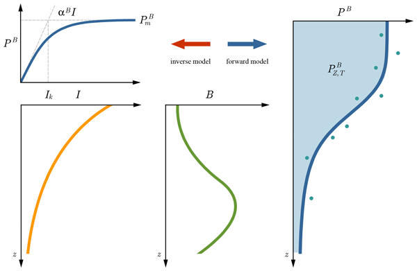
where P^B is the biomass normalised production and the notation p^B marks the photosynthesis irradiance function (Fig. 1). There are numerous such functions in oceanographic usage, with a rich history of applications (Zonneveld, 1998; Kovač et al., 2017b). All functions are expressible using two parameters: the initial slope α^B and the assimilation number $P_m^B$ (Platt et al., 1977; Frenette et al., 1993; Behrenfeld et al., 2004), which we write as:

$$\begin{array}{}\text{(2)}& P^B=p^B\left(I\right|{\mathit{\alpha }}^B,P_m^B).\end{array}$$

Here, the initial slope α^B describes the linear response of primary production at low light, whereas the assimilation number $P_m^B$ describes the rate of primary production at saturating light intensities (MacIntyre et al., 2002; Falkowski, 1981; Milligan et al., 2015). A third parameter, defined as a ratio of the assimilation number and the initial slope, is the photoadaptation parameter:

$$\begin{array}{}\text{(3)}& I_k={\displaystyle \frac{P_m^B}{{\mathit{\alpha }}^B}}.\end{array}$$

The photoadaptation parameter describes how phytoplankton adjust their light-harvesting capacity to ambient light conditions (Reynolds, 2006; Kirk, 2010). It represents the irradiance at which phytoplankton transition from light limited to light saturated photosynthesis (Jassby and Platt, 1976) and is also a measure of the light level to which phytoplankton have adapted (Zonneveld, 1997).

Figure 1 Graphical representation of the relation between the forward and inverse models. Both models are based on a functional relationship between normalized production and light, expressed using photosynthesis irradiance functions (top left). These functions require information on the photosynthesis parameters: the initial slope α^B and the assimilation number $P_m^B$, which are typically estimated from in vitro photosynthesis irradiance experiments. With information on the biomass profile (green curve, bottom middle) and underwater irradiance (orange curve, bottom left) a forward model calculates the daily production profile (blue curve on the right) and watercolumn production (blue surface on the right). An inverse model does the opposite. With an in situ measured production profile (green dots) an inverse model estimates the values of the photosynthesis parameters by minimizing the error between the model prediction (blue curve) and the measurements (green dots).

In the ocean, irradiance is a function of both depth z and time t and a light penetration model is required to calculate $I=I(z,t)$ (Kirk, 2010). Keeping in mind the limitations of the Mattei and Scardi (2021a) dataset, namely a single value for the attenuation coefficient K and a peak value at solar noon for irradiance $I_{\mathrm{0}}^m$, we employ a relatively simple light penetration model:

$$\begin{array}{}\text{(4)}& I(z,t)=I_{\mathrm{0}}^m\sin \left(\mathit{\pi }t/D\right)\exp (-Kz),\end{array}$$

where D is daylength (time from sunrise till sunset). Knowing the underwater irradiance (Eq. 4) and the response of primary production to it (Eq. 2), enables the calculation of primary production per unit biomass, for a given depth and time, as $P^B(z,t)=p^B\left(I\right(z,t\left)\right)$. To calculate primary production, additional information on biomass at depth is needed, which is specified as B(z), and typically taken as constant during one day (but see Kovač et al., 2017a). Multiplication of normalised production by biomass and integration over daylength yields the daily production profile P_T(z):

$$\begin{array}{}\text{(5)}& P_T\left(z\right)=B\left(z\right)\underset{\mathrm{0}}{\overset{D}{\int }}{p}^B\left(I\left(z,t\right)\right)\mathrm{d}t,\end{array}$$

which is the model analogue of the in situ measured production profile (Kovač et al., 2016b). By further integration over depth we obtain daily watercolumn production as:

$$\begin{array}{}\text{(6)}& P_{Z,T}=\underset{\mathrm{0}}{\overset{\mathrm{\infty }}{\int }}{P}_T\left(z\right)\mathrm{d}z.\end{array}$$

The two integrals are typically solved numerically, but for the Platt et al. (1980) photosynthesis irradiance function, both have been solved analytically. The exact solution for watercolumn production with uniform biomass is provided by Platt et al. (1990), whereas solutions for the case of non-uniform biomass profiles can be found in Kovač et al. (2017a). The analytical solution for the daily production profile is given in Kovač et al. (2016b), with a summary of other analytical solutions provided in Kovač et al. (2017b). In the context of parameter estimation both Eqs. (5) and (6) would be referred to as forward models, in the sense that for given parameter values the model calculates a primary production profile and watercolumn production (Fig. 1). The opposite procedure to this, namely estimation of parameters from a known production profile, is referred to as an inverse procedure, or an inverse model (Fig. 1). Details of the forward and inverse models used in this study are given in Appendices B and C, respectively.

To extract the values of photosynthesis parameters given a measured in situ production profile, we first normalize the production profile (Eq. 5) with biomass, to get at the normalised daily production profile (Kovač et al., 2016b), which we recognize is also a function of parameter values themselves, written in analogy with Eq. (2), as:

$$\begin{array}{}\text{(7)}& P_T^B\left(z\right)=P_T^B\left(z\right|{\mathit{\alpha }}^B,P_m^B).\end{array}$$

Now, for a given survey from the Mattei and Scardi (2021a) dataset we obtain by measurement the following variables: biomass profile $\stackrel{\mathrm{̃}}{B}\left(z_n\right)$ and daily production profile ${\stackrel{\mathrm{̃}}{P}}_T\left(z_n\right)$, both at a sequence of depths z_n, along with noon irradiance ${\stackrel{\mathrm{̃}}{I}}_{\mathrm{0}}^m$ and the attenuation coefficient $\stackrel{\mathrm{̃}}{K}$, complemented with daylength $\stackrel{\mathrm{̃}}{D}$. We use the tilde ∼ to indicate a measured variable, whereas without tilde, the variable refers to the model.

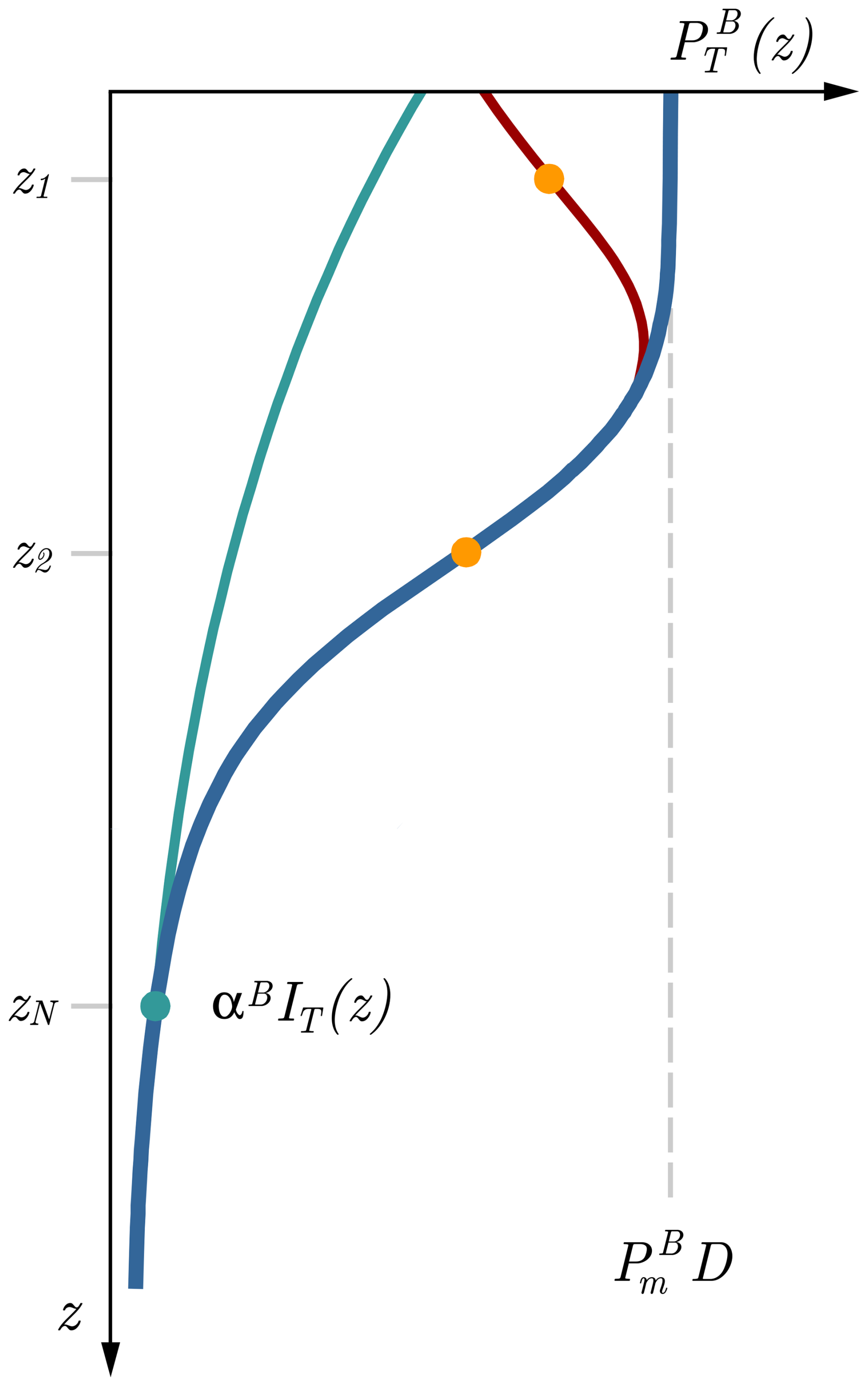
Figure 2 The starting estimate for the value of the assimilation number can be estimated from measured surface values of primary production by assuming saturation close to the surface (grey dashed line). The in situ production measurements carried out close to the ocean surface (orange dot at depth z₁) may experience photoinhibition due to exposure to high irradiance (irradiance profile given in green). This will cause a dip in the production profile (red curve) close to the surface from what would otherwise be a saturating profile (blue curve). Likewise, the starting estimate for the initial slope can be estimated from measurements at great depth where saturation of photosynthesis does not take place during the experiment (green dot).

To be more precise, from measurements we obtain, for a given survey, a sequence of pairs: $\stackrel{\mathrm{̃}}{B}\left(z_n\right)$ and ${\stackrel{\mathrm{̃}}{P}}_T\left(z_n\right)$, at depths z_n, with $n=\mathrm{1},\mathrm{2},\mathrm{\dots },N$, and N being the total number of measurement depths for a given survey. For each depth z_n, by dividing measured daily production ${\stackrel{\mathrm{̃}}{P}}_T\left(z_n\right)$ by the measured biomass, $\stackrel{\mathrm{̃}}{B}\left(z_n\right)$ we get the measured normalised daily production profile as:

$$\begin{array}{}\text{(8)}& {\stackrel{\mathrm{̃}}{P}}_T^B\left(z_n\right)={\stackrel{\mathrm{̃}}{P}}_T\left(z_n\right)/\stackrel{\mathrm{̃}}{B}\left(z_n\right).\end{array}$$

To estimate the values of photosynthesis parameters, the model normalised production profile (7) is compared with the measured normalised production profile (8). To help constrain the model we also compare the modelled and measured normalised watercolumn production. Model normalised watercolumn production is given as:

$$\begin{array}{}\text{(9)}& P_{Z,T}^B=\underset{\mathrm{0}}{\overset{\mathrm{\infty }}{\int }}{P}_T^B\left(z\right)\mathrm{d}z,\end{array}$$

and measured normalised watercolumn production as:

$$\begin{array}{}\text{(10)}& {\stackrel{\mathrm{̃}}{P}}_{Z,T}^B=\sum _{n=\mathrm{1}}^N{\stackrel{\mathrm{̃}}{P}}_T^B\left(z_z\right)\mathrm{\Delta }{z}_n,\end{array}$$

where Δz_n is the depth interval associated with each measurement depth (see Appendix C). Quantification of the model data mismatch is defined with the following optimal function as:

$$\begin{array}{}\text{(11)}& \begin{array}{rl}\mathcal{P}({\mathit{\alpha }}^B,P_m^B)& =\sum _{n=\mathrm{1}}^N{\left(P_T^B\left(z_n\mid {\mathit{\alpha }}^B,P_m^B\right)-{\stackrel{\mathrm{̃}}{P}}_T^B\left(z_n\right)\right)}^{\mathrm{2}}\\ & +{\left(P_{Z,T}^B\left({\mathit{\alpha }}^B,P_m^B\right)-{\stackrel{\mathrm{̃}}{P}}_{Z,T}^B\right)}^{\mathrm{2}},\end{array}\end{array}$$

which is a function of photosynthesis parameters. The first term takes into account the shape of the measured production profile (green dots on the right in Fig. 1), while the second term takes into account normalised watercolumn production (blue surface on the right in Fig. 1). Now, the problem of estimating photosynthesis parameters from measured production profiles is reduced to finding the minimum of this function (Kovač et al., 2016b, a). Optimization methods for achieving this, as well as the technical details of the forward and inverse model are provided in Appendices B and C. The inverse model is applied for each profile on its own, from which photosynthesis parameters are estimated. We label the estimated values of photosynthesis parameters as: ${\widehat{\mathit{\alpha }}}^B$ and ${\widehat{P}}_m^B$, where this notation is used specifically to denote estimated parameter values. This procedure is repeated over the entire Mattei and Scardi (2021a) dataset, which yields the new dataset of photosynthesis parameters. But prior to the application, we first describe the limitations of the approach, which stem from data and model limitations.

The first limitation stems from the optical data requirements, where the inverse method requires data on surface irradiance and the attenuation coefficient, in addition to the biomass and production profiles. Such data is not always readily available, but in the inverse model both parameters can, in principle, be estimated without independent information on irradiance or the attenuation coefficient (Kovač et al., 2016a). However, because of the model structure, the estimates of surface irradiance and the attenuation coefficient, which together describe the irradiance profile, would then not be independent of the estimate of the initial slope by the inverse model (Kovač et al., 2017b). Specifically, the initial slope and irradiance always occur as a product in the forward model (Appendix B). Consequently, accurate estimation of the initial slope requires reliable information on both surface irradiance and the attenuation coefficient. In contrast, the estimate of the assimilation number is largely unaffected by this dependency. This is because the assimilation number is predominantly constrained by incubations conducted near the surface, where photosynthesis is saturated with light for most of the day. The initial slope, on the other hand, is determined mainly from incubations conducted at greater depths, making its estimate more sensitive to the accuracy of the underwater irradiance profile.

The strongest limitation on the inverse approach comes from the assumption of vertical homogeneity in photosynthesis parameters. This implies that one value of the initial slope α^B and one value of the assimilation number $P_n^B$ is assigned to phytoplankton throughout the entire water column. In the ocean, photosynthesis parameters may, and likely do vary vertically, especially in case of strong stratification (Bouman et al., 2018). Also, temporally, phytoplankton are known to adjust values of photosynthesis parameters over the course of a few generations (Reynolds, 2006). However, the time scale of in situ incubations is of the order of one day, therefore it is unlikely that significant changes will occur within the duration of the experiment. In principle, if there were numerous measurements carried out in the vertical, such that the production and biomass profiles were resolved well vertically, a more complex model with vertically varying photosynthesis parameters could be used. The same reasoning would apply if numerous shorter incubations were carried out during the day.

A direct mathematical consequence of vertically uniform photosynthesis parameters is the constraints on the application range of the model. In the case of uniform photosynthesis parameters, the normalised daily production profile is a declining function of depth (Fig. 2):

$$\begin{array}{}\text{(12)}& {\displaystyle \frac{\partial P_T^B\left(z\right)}{\partial z}}<\mathrm{0}.\end{array}$$

Therefore, the model can only be expected to work well for in situ normalised production profiles which also decline with depth. This is easy to test by simply observing whether:

$$\begin{array}{}\text{(13)}& {\stackrel{\mathrm{̃}}{P}}_T^B\left(z_n\right)>{\stackrel{\mathrm{̃}}{P}}_T^B\left(z_{n+\mathrm{1}}\right).\end{array}$$

We should also stress that measurements near the surface, as shown in Fig. 2, may be prone to photoinhibition: a reduction of primary production at high irradiance (Marshall et al., 2000). The reduction of primary production due to photoinhibition is likely to occur if the incubations are carried out for prolonged periods of time under high irradiance (Ross et al., 2011b, a). In the ocean, phytoplankton are free floating and are continually being circulated in the mixed layer, whereas for in situ incubations the experiments are carried out at fixed depths. This implies mixing is prevented and phytoplankton which would otherwise be freely mixed, are now exposed to significantly higher irradiance, which may lead to light stress. Signs of photoinhibition are easily observed in the normalised production profile by testing whether normalised daily production at the first measurement depth is less than that measured at the subsequent depths (Fig. 2). Given that photoinhibition occurs close to the surface, its effect on watercolumn production is expected not to be pronounced (Platt et al., 1990; Ross et al., 2011b).

Further more, to enable faster and more accurate estimation of optimal photosynthesis parameters, initial values in the optimization procedure need to be specified (Kovač et al., 2016a). For the initial value of the assimilation number, we note first that saturation of photosynthesis is more likely close to the surface, but not at the first measurement depth, since that is where photoinhibition might occur. At the second measurement depth, it is more likely that photoinhibition will not be pronounced and we can assume that during most of the incubation's duration primary production at this depth will be close to saturation for most of the day, except when light levels drop towards zero at dawn and dusk (Fig. 2). Therefore, we can approximate daily normalised production at the second depth as:

$$\begin{array}{}\text{(14)}& {\stackrel{\mathrm{̃}}{P}}_T^B\left(z_{\mathrm{2}}\right)\approx P_m^{B}D.\end{array}$$

This assumption leads easily to the starting value for the assimilation number (Fig. 2), which we label as $(P_m^B{)}_{\mathrm{0}}$:

$$\begin{array}{}\text{(15)}& (P_m^B{)}_{\mathrm{0}}={\displaystyle \frac{{\stackrel{\mathrm{̃}}{P}}_T^B\left(z_{\mathrm{2}}\right)}{D}}.\end{array}$$

Likewise, the starting value of the initial slope can also be approximated from the production profile. At great depth, photosynthesis will likely remain unsaturated for the duration of the incubation and production will depend on irradiance linearly. This implies that we can approximate daily normalised production at the final depth z_N, provided it is optically deep enough, as:

$$\begin{array}{}\text{(16)}& P_T^B\left(z_N\right)\approx {\mathit{\alpha }}^B{I}_T{e}^{-K{z}_N},\end{array}$$

where I_T is the daily integral of surface irradiance (Fig. 2). From this we can express the starting value of the initial slope as:

$$\begin{array}{}\text{(17)}& ({\mathit{\alpha }}^B{)}_{\mathrm{0}}={\displaystyle \frac{P_T^B\left(z_N\right)}{I_T{e}^{-K{z}_N}}}.\end{array}$$

Having the starting values for both the assimilation number and the initial slope, helps speed up the search process for the optimal parameter values. It also aids in preventing the optimization algorithm from ending up in a local minima of the error function (11), instead of the global minima. With the inverse model described, we now proceed to describe the dataset.

Figure 3 Map of the in situ production profiles from the Mattei and Scardi (2021a) dataset (orange dots). In total there are 6084 biomass and production profiles in the dataset. Most of the data come from the Northern Hemisphere. The data were collected from 1958 till 2017, with the total of 37 722 individual measurements of biomass and primary production pairs. Also shown is the published archive of photosynthesis parameters by Bouman et al. (2018), which contains 5711 values of photosynthesis parameters globally in the time spam from 1977 to 2013 (green dots). The Mattei and Scardi (2021a) dataset complements the Bouman et al. (2018) dataset by covering areas in which no photosynthesis parameters were published, creating an incentive for photosynthesis parameters estimation from in situ production profiles.

3 Production profiles dataset

The Mattei and Scardi (2021a) dataset contains primary production profiles measured in situ and distributed throughout the global ocean as shown in Fig. 3. The authors have compiled the dataset by complementing the already existing dataset from the Oregon State University, which at the time consisted of 2214 production profiles. This dataset was used in the development of the Vertically Generalized Production Model (Behrenfeld and Falkowski, 1997b, a). It was then supplemented by Mattei and Scardi (2021a) with additional 3870 profiles from the world oceans.

The Mattei and Scardi (2021a) dataset contains 6084 individual production profiles measured from 1958 till 2017, with the total of 37722 individual pairs of measurements of primary production and biomass. The vast majority (5578) of the profiles are from the Northern Hemisphere (Fig. 3), whereas only 478 are located in the Southern Hemisphere and 28 are classified as Equator profiles. Over the seasonal cycle, the authors report: 1701 for winter, 1802 for spring, 1589 for summer and 992 for autumn, which is a relatively uniform annual coverage. The full dataset contained 3756 profiles with measured surface photosynthetically active radiation (PAR), whereas the missing PAR were filled with satellite estimates by Mattei and Scardi (2021a) (see second section in their paper for details on the gap filling approach). PAR was provided in units of E m⁻²d⁻¹ and the conversion to W m⁻² was done using Smith and Morel's procedure (Morel and Smith, 1974). Surface noon irradiance $I_{\mathrm{0}}^m$ was subsequently determined as ${\stackrel{\mathrm{̃}}{I}}_{\mathrm{0}}^m={\stackrel{\mathrm{̃}}{I}}_{\mathrm{T}}\mathit{\pi }/\mathrm{2}D$, where ${\stackrel{\mathrm{̃}}{I}}_{\mathrm{T}}$ is the total received irradiance during daylength. Note that this conversion assumes a sine function for the time-dependent variation of irradiance over the daylength, which is consistent with the model used here, namely Eq. (4) (see also Platt et al., 1990). For the profiles without measured PAR, Mattei and Scardi (2021a) have performed gap filling from 2003 onwards. The authors have also performed gap filling of missing biomass and production data with depth weighted averages of the closest measured values.

The essential variables needed to estimate photosynthesis parameters from in situ experiments are: biomass profile, primary production profile, surface photosynthetically active radiation and the diffuse attenuation coefficient for downwelling irradiance. These are all given in the dataset. To be more precise, the euphotic zone depth Z_e is given in the dataset, with the calculation of the attenuation coefficient done simply as $\stackrel{\mathrm{̃}}{K}=\ln \left(\mathrm{100}\right)/Z_{\mathrm{e}}$. The dataset also contains auxiliary variables for each experiment, such as: day, month, year, latitude and longitude, euphotic zone depth, mixed layer depth, bottom depth, distance from coastline, as well as many other variables. See the Supplement from the Mattei and Scardi (2021a) paper for details on the dataset. The full dataset is available on the PANGAEA repository via the following link: https://doi.org/10.1594/PANGAEA.932417 (Mattei and Scardi, 2021b).

The auxiliary variables enable us to ascertain the adequacy of the dataset for the inverse model. From the standpoint of photosynthesis parameter estimation, it is important to know the range of irradiance experienced by the phytoplankton during the incubations (Kovač et al., 2016a), which can be ascertained by expressing the measurement depth of each experiment as an optical depth ζ, as show in Fig. 4a. From the distribution of the measurement frequency as a function of optical depth we observe that most of the measurements are carried out at shallow optical depths. As the optical depth increases the number of measurements drops off. This is expected, given primary production measurements are typically performed within the euphotic zone (corresponding to ζ=4.6).

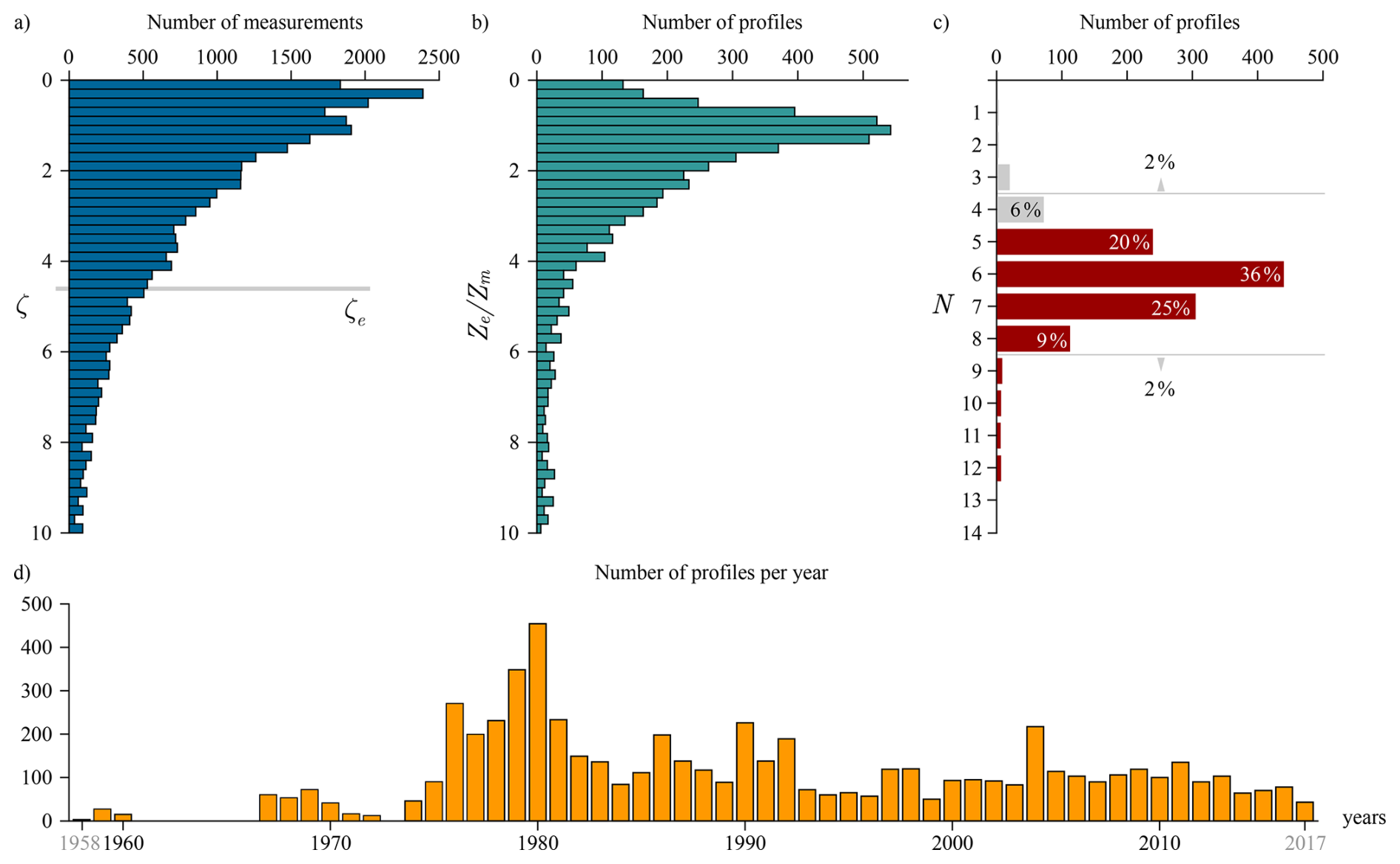
Figure 4 Plots of auxiliary variables. (a) Histogram of measurement depths expressed as optical depths. Each individual measurement is treated as one entry. Euphotic zone ζ_e is highlighted by the grey line. (b) Histogram of the ratio between the euphotic depth and the mixed layer depth. Here each profile is treated as one entry. (c) Histogram of profiles with a given number of measurement depths. The two grey arrows indicate that percentages refer to all the profiles below or above the grey line. (d) Time series of the number of measured production profiles per year globally.

In fact, after the estimation of optimal photosynthesis parameters, it is possible to partition the water column into depths for which I(z)>I_k, and depths for which I(z)<I_k. Nominally, for depths that meet the first criterion, production would be determined by $P_m^B$, and for the latter case, production would be determined by α^B (Kovač et al., 2016a). For the limited case of application to computation of watercolumn production (which is the case dealt with, here), the importance is to get $P_m^B$ right for depths that lie above the I(z)=I_k depth horizon, and to get α^B right for depths below that horizon. For this reason it is important that the incubations are carried out over a range of optical depths.

Another important indicator for inverse model applicability is the value of the mixed layer depth relative to euphotic depth for each station, shown in Fig. 4b. Here we observe that for most of the profiles mixed layer depth was of the same order of magnitude as the euphotic depth. This implies probable vertical homogeneity in photosynthesis parameters for the given incubations. The highest number of profiles has the mixed layer depth almost equal to the euphotic depth, which is also a good indicator for the justification of vertical homogeneity of photosynthesis parameters.

Finally, for the inverse model to be able to estimate the values of photosynthesis parameters, the measured production profile has to have a minimal number of depths to vertically resolve the shape of the normalised production profile. As demonstrated by Kovač et al. (2016a) the normalised production profile (Eq. 7) is uniquely determined by the photosynthesis parameters, whereas normalised daily watercolumn production (Eq. 9) is not. This is because the normalised watercolumn production is an integral of the normalised production profile (Fig. 1) and therefore loses the degrees of freedom that are present in the production profile, which enable the estimation of photosynthesis parameters. Therefore, a given pair of photosynthesis parameters may not be an exact match for the normalised production profile, but it may be a good match for watercolumn production.

We have analysed the distribution of profiles with respect to the number of measurement depths per profile, as shown in Fig. 4c. The highest number of profiles has 6 measurement depths, which is adequate for successful parameter estimation. The total number of profiles with 6 or more measurement depths accounts for 72 % of the measured profiles. Around 20 % of the profiles have 5 measurement depths, which is on the limit for successful parameter estimation. In order to use as much of the available data as possible, we have opted to use these profiles as well in parameter estimation. The remainder 8 % of profiles have less than 5 measurement depths. In other words, out of the 6084 profiles, 473. For these profiles, it is not feasible to estimate both parameters, and therefore we opted to exclude them. On the other end, some profiles have measurements from 9 to 14 depths (which is excellent), but these account for less than 2 % of all the profiles.

Looking at the temporal distribution of measurements, as shown in Fig. 4d, the observations start in 1958, but there is a gap from 1961 till 1966, with another gap year in 1973. After 1975, there is a surge in data collection, with the highest number of profiles being measured in 1980 and in the neighbouring years. Afterwards, the global number of measured profiles is of the order of 100 yr⁻¹. This is arguably very low, highlighting the value of such measurements, given the high demand for photosynthesis parameters in remote sensing applications and in ecosystem models. With this in mind, we now proceed to describe the application of the inverse model and the obtained results.

4 Results

As a first step in the application of the inverse model we have analysed primary production profiles for signs of vertical homogeneity in photosynthesis parameters, by testing whether they meet condition (Eq. 13), and if so for how many depths. Out of the total 5611 profiles with more than 4 measurement depths, 988 profiles do not violate this condition at all, 2407 profiles violate it at one depth, 1469 at two depths and 747 at three or more depths. We have at first applied the inverse model on all profiles only to find that those profiles which strongly violate the vertical homogeneity condition result in outlier values for photosynthesis parameters. Therefore, we focus on those profiles for which the vertical homogeneity condition is not violated, or violated at one or two depths. In total there are 4864 such profiles. This accounts for 80 % of the original 6084 profiles in the Mattei and Scardi (2021a) dataset.

Distributions of photosynthesis parameters obtained from these profiles are provided in Fig. 5. The obtained parameter values are within the expected ranges thus far reported in the literature (Kovač et al., 2017b; Bouman et al., 2018; Amirian et al., 2025). The estimated values of the initial slope α^B range from above zero to 0.60 mg C (mg Chl)⁻¹ (W m⁻²)⁻¹ h⁻¹, with only a handful parameter values above the upper limit. The majority of values of the assimilation number $P_m^B$ are found to be below 10.00 mg C (mg Chl)⁻¹ h⁻¹, with the bulk of the estimates being above zero and below 5.00 mg C (mg Chl)⁻¹ h⁻¹, consistent with conventional photosynthesis-irradiance experiments. Neither of these parameters are normally distributed, being positively skewed and exhibiting long tails. The mean and median of the inital slope α^B being 0.19 and 0.13 mg C (mg Chl)⁻¹ (W m⁻²)⁻¹ h⁻¹, respectively, with the mean and median of the assimilation number $P_m^B$ begin 4.32 and 2.74 mg C (mg Chl)⁻¹ h⁻¹, respectively. From the information on the values of the initial slope and the assimilation number it is straightforward to calculate the photoadaptation parameter (3). Distribution of the photoadaptation parameter is also given in Fig. 5. It is positively skewed with a long tail. The bulk of the photoadaptation parameter values are found below 50.00 W m⁻². The mean and the median of the photoadaptation parameter I_k are 20.86 and 11.62 W m⁻², respectively.

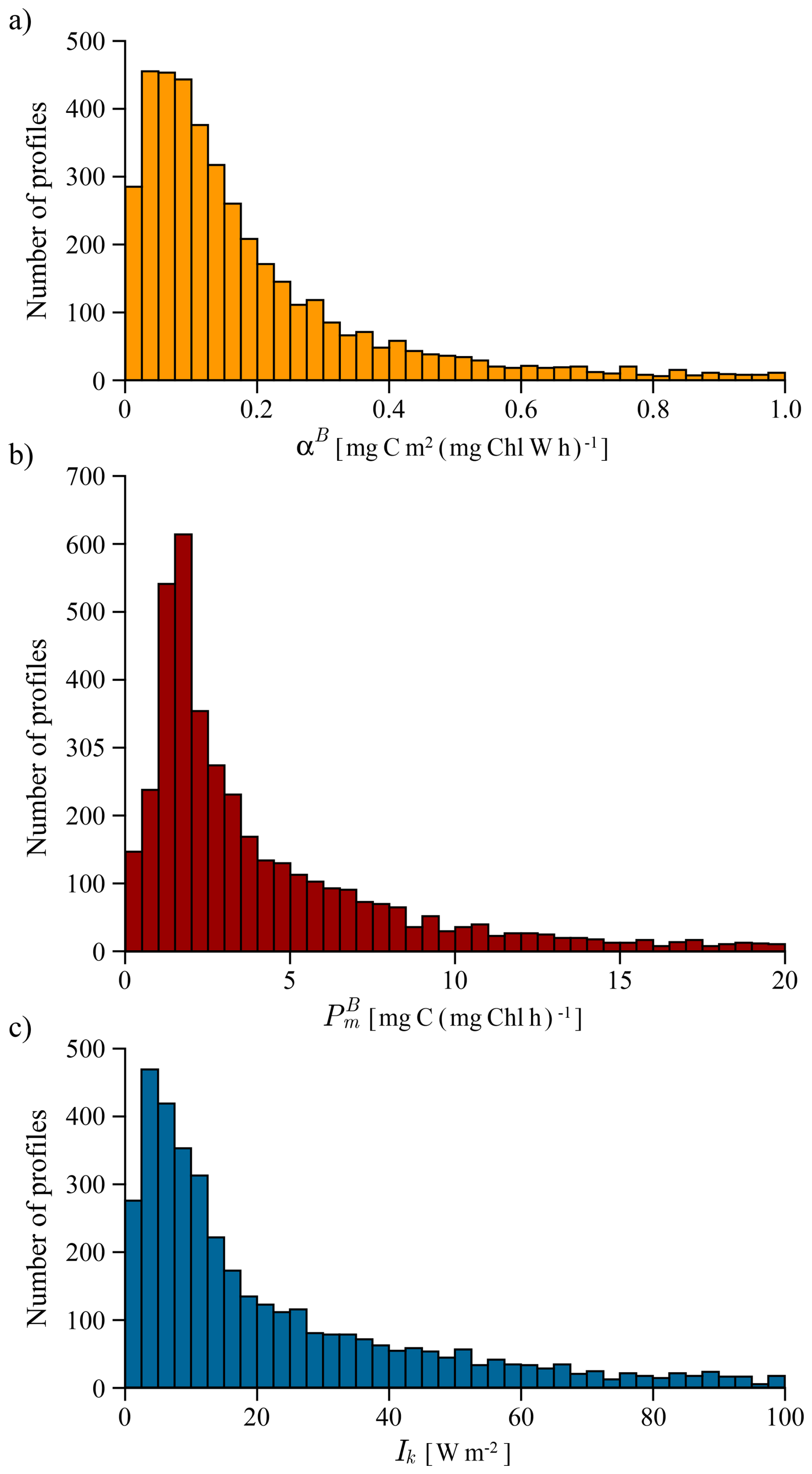
Figure 5 Histograms of the estimated photosynthesis parameters: (a) Distribution of the initial slope α^B, (b) Distribution of the assimilation number $P_m^B$, (c) Distribution of the photoadaptation parameter I_k. The horizontal axis shows parameter values, and the vertical axis indicates the number of profiles within each interval of those values.

We stress here that the objective of this study was not to provide an interpretation of this specific dataset, but rather to increase the number of photosynthesis parameters available for usage in primary production models. A comprehensive interpretation of the estimated parameter values would necessitate a detailed oceanographic analysis and knowledge of regional, or local biogeochemical processes, which falls outside the scope of the present work and is a potential course for future research. To facilitate this, we provide the obtained parameter values in a table published online at https://doi.org/10.5281/zenodo.17973417 (Kovač et al., 2025). Along with each estimated pair of photosynthesis parameters we provide the original profile number given by Mattei and Scardi (2021a) so that the parameter values can be traced back to the profiles from which they had been estimated. We also give the date of each profile, along with coordinates. To be more precise the data are comprised of the following: date (year, month, day), latitude, longitude, initial slope α^B, assimilation number $P_m^B$ and the original profile number from Mattei and Scardi (2021a), each given in a separate column. There are also instances where one parameter value is estimated, but the other is not, due to insufficient information in the measured primary production profiles to reliably estimate both parameters. Therefore, we only published parameter pairs in which values of both parameters were estimated successfully, in line with the limitations set by the experiment and the inverse procedure, described in detail in Kovač et al. (2016a). We also flag the values where the inverse procedure did not result in realistic values of photosynthesis parameters with 0, the ones where the initial slope is too high with 0.5 and the realistic values with 1.

In the provided table, parameter values for which the inverse model did not converge onto realistic values are flagged and given as NaN. In some of these cases the model did yield reasonable estimates for watercolumn production, but for unrealistic values of photosynthesis parameters. This occurs due to the fact that watercolumn production is not uniquely determined by the photosynthesis parameters, but the production profile is (Kovač et al., 2016a). Therefore, the method may converge on a combination of parameter values for which watercolumn production is estimated rather well, but the production profile is not. In short, for those cases, the model gives the correct answer for watercolumn production, but for the wrong reasons. Keeping in mind the parameter values are estimated from the shape of the production profile we consider the error in the profile to take precedence. Another reason for plausible divergence in the values of photosynthesis parameters is the potential lack of information in the shape of the production profile to estimate both parameters. Under certain irradiance conditions, and based on the optical depths at which the incubations have been carried out, there may only be sufficient information on one parameter to be estimated (Kovač et al., 2016a). If this is the case, the value of the other parameter is not uniquely determined by the measured production profile and the inverse model estimate of that parameter value can diverge. In such instances the parameter values were also flagged.

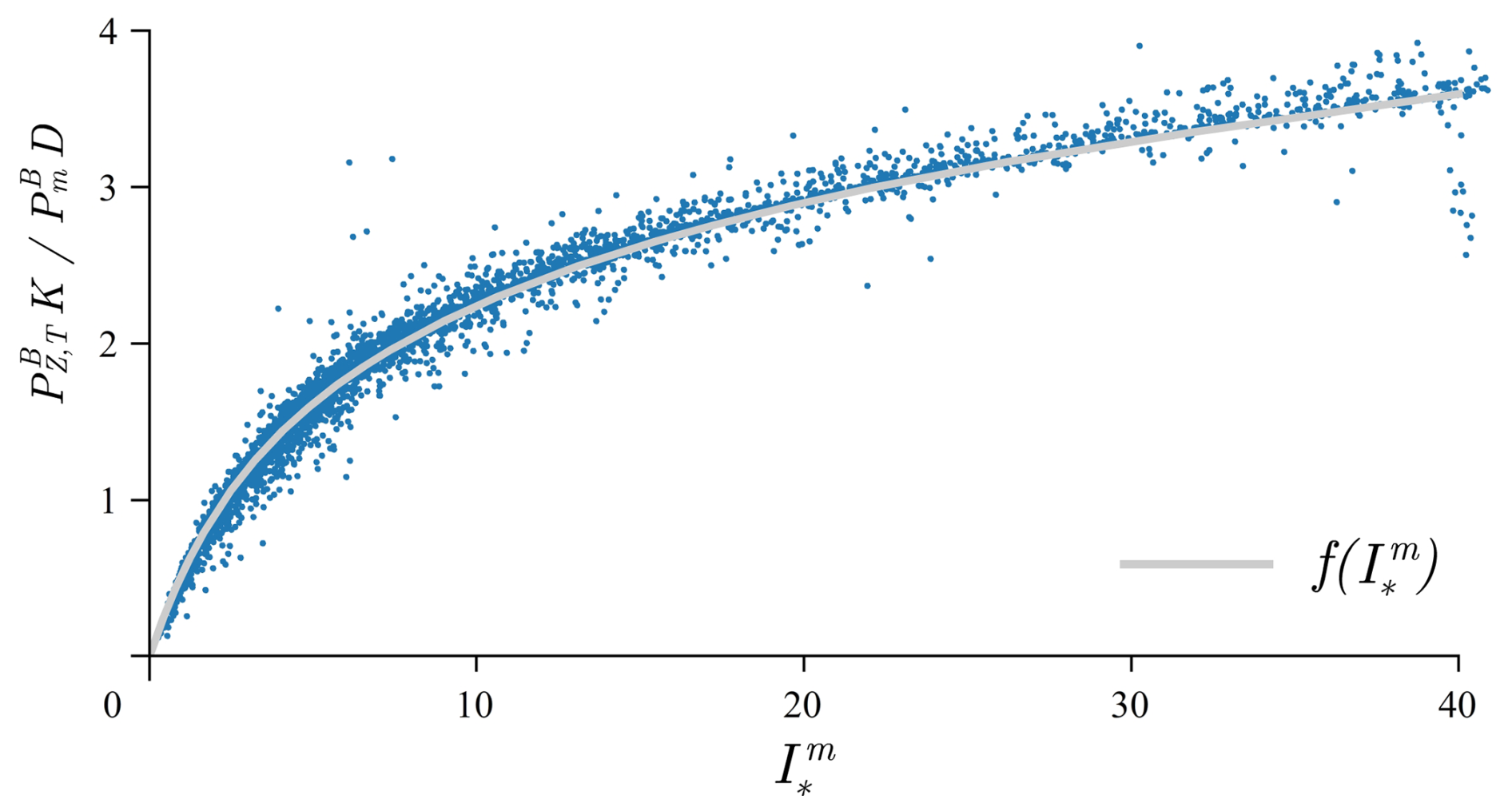
Figure 6 Comparison of measured normalised watercolumn production versus the analytical solution for normalised daily watercolumn production (Eq. 18) by Platt et al. (1990). The abscissa represents the dimensionless noon irradiance $I_{*}^m$ (Eq. 19) while the ordinate gives the normalised watercolumn production divided by $P_m^{B}D/K$. The solid curve corresponds to the $f\left(I_{*}^m\right)$ function. In total, there are X profiles plotted.

The estimated photosynthesis parameters allows us to further calculate goodness of fit, which to the best of our knowledge has not been done thus far on such a large in situ dataset. Goodness of fit can be tested on normalized watercolumn production as well as on watercolumn production. Of primary interest in remote sensing applications would be the latter, whereas for parameter estimation the former is of higher importance. Before presenting goodness of fit, we should highlight that similar analysis have been performed by Behrenfeld and Falkowski (1997a) on the Ocean productivity dataset, which at the time of publication in 1997 had 10 857 individual incubations (their Fig. 4). That dataset is now a subset of the Mattei and Scardi (2021a) dataset, which holds 37 722 individual incubations, whilst keeping most of the Behrenfeld and Falkowski (1997a) data within it. The details on which data from Behrenfeld and Falkowski (1997a) are included in the the Mattei and Scardi (2021a) dataset is provided in their paper.

To present the overall model goodness of fit in calculating watercolumn production, we use the estimated parameter values to normalize the data and compare it to the Platt et al. (1990) analytical solution for watercolumn production, following the procedure described in Kovač et al. (2016b). For the Platt et al. (1980) photosynthesis irradiance function, used in this work, exact analytical solution for normalised watercolumn production can be written as:

$$\begin{array}{}\text{(18)}& P_{Z,T}^B={\displaystyle \frac{P_m^{B}D}{K}}f\left(I_{*}^m\right),\end{array}$$

where:

$$\begin{array}{}\text{(19)}& I_{*}^m={\displaystyle \frac{{\mathit{\alpha }}^B{I}_{\mathrm{0}}^m}{P_m^B}},\end{array}$$

is the normalised noon irradiance and $f\left(I_{*}^m\right)$ a known function (see Appendix B). By rewriting the above expression as:

$$\begin{array}{}\text{(20)}& {\displaystyle \frac{K{P}_{Z,T}^B}{P_m^{B}D}}=f\left({\displaystyle \frac{{\mathit{\alpha }}^B{I}_{\mathrm{0}}^m}{P_m^B}}\right),\end{array}$$

and using the estimated parameter values ${\widehat{\mathit{\alpha }}}^B$ and ${\widehat{P}}_m^B$, along with noon irradiance ${\stackrel{\mathrm{̃}}{I}}_{\mathrm{0}}^m$, enables the calculation of $I_{*}^m$, which is the argument of the f function on the right hand side. On the left hand side, daylength D is known for each measured profile and the attenuation coefficient is measured $\stackrel{\mathrm{̃}}{K}$. From the measured normalised production profile ${\stackrel{\mathrm{̃}}{P}}_T^B\left(z_n\right)$ (Eq. 8), normalised watercolumn production is easily calculated using the trapezoidal rule. Therefore, the left hand side is known. This further enables the comparison of the $f\left(I_{*}^m\right)$ function with the entire dataset, by simply plotting the data as ordered pairs $({\widehat{\mathit{\alpha }}}^B{\stackrel{\mathrm{̃}}{I}}_{\mathrm{0}}^m/{\widehat{P}}_m^B,\stackrel{\mathrm{̃}}{K}{\stackrel{\mathrm{̃}}{P}}_{Z,T}^B/{\widehat{P}}_m^{B}D)$ on the same plot as $f\left(I_{*}^m\right)$. Details on this procedure are provided in Kovač et al. (2016b). The results are given in Fig. 6.

To further quantify model performance we have used additional statistical measures following Li et al. (2022). The mathematical expressions for these statistical measures are provided in Appendix D. We have calculated the coefficient of determination R², the root mean square difference RMSD, the unbiased absolute percentage difference UAPD and the logarithmic bias LB. We got the following results for our model in case of watercolumn production P_Z,T: R²=82.01 %, RMSD =0.208, UAPD =33.48 % and LB =10.40 %. Subsequently, we got the following results for our model in case of normalized watercolumn production $P_{Z,T}^B$: R²=70.05 %, RMSD =0.240, UAPD =35.49 % and LB =4.58 %.

In comparison to Kovač et al. (2016b) the optimal function used here (Eq. 11) has the additional constraint on normalised watercolumn production. This helps the inverse model to come close to the measured estimate of normalised watercolumn production, while simultaneously describing the production profile. Upon testing the inverse model we have found this to be advantageous, as it prevents it from diverging in numerous cases. It also aided in constraining the estimate of watercolumn production, by balancing the estimate of production at depth alongside watercolumn production. The benefit from simultaneously constraining watercolumn production and production at all measured depths was most pronounced with profiles having a small number of measurement depths.

5 Discussion

In contemporary oceanography, estimation of global primary production is carried out using remote sensing algorithms (Westberry et al., 2023) and biogeochemical models (Follows et al., 2007). In both, primary production is calculated using parameters that describe the response of phytoplankton photosynthesis to available light. This response is described mathematically using photosynthesis irradiance functions (Platt and Jassby, 1976; Jones et al., 2014). These functions are uniquely determined by two parameters: the initial slope and the assimilation number, together termed the photosynthesis parameters (Sakshaug et al., 1997). Unlike other essential parameters and variables that are used in primary production models, such as chlorophyll a, attenuation coefficient and photosynthetically available radiation, photosynthesis parameters are unfortunately not easily amenable to remote sensing, making photosynthesis parameter assignment a bottleneck in global primary production models. Given that global calculations of primary production are very sensitive to photosynthesis parameters (Platt et al., 1988; Kulk et al., 2020, 2021) and given we cannot regularly estimate them by remote sensing, the increase in spatio-temporal coverage in photosynthesis parameters becomes a priority. In line with this, active research on photosynthesis irradiance functions and novel methods for parameter estimation, with the aim of refining models and increasing the availability of photosynthesis parameters, is still ongoing (Amirian et al., 2025; Britten et al., 2025).

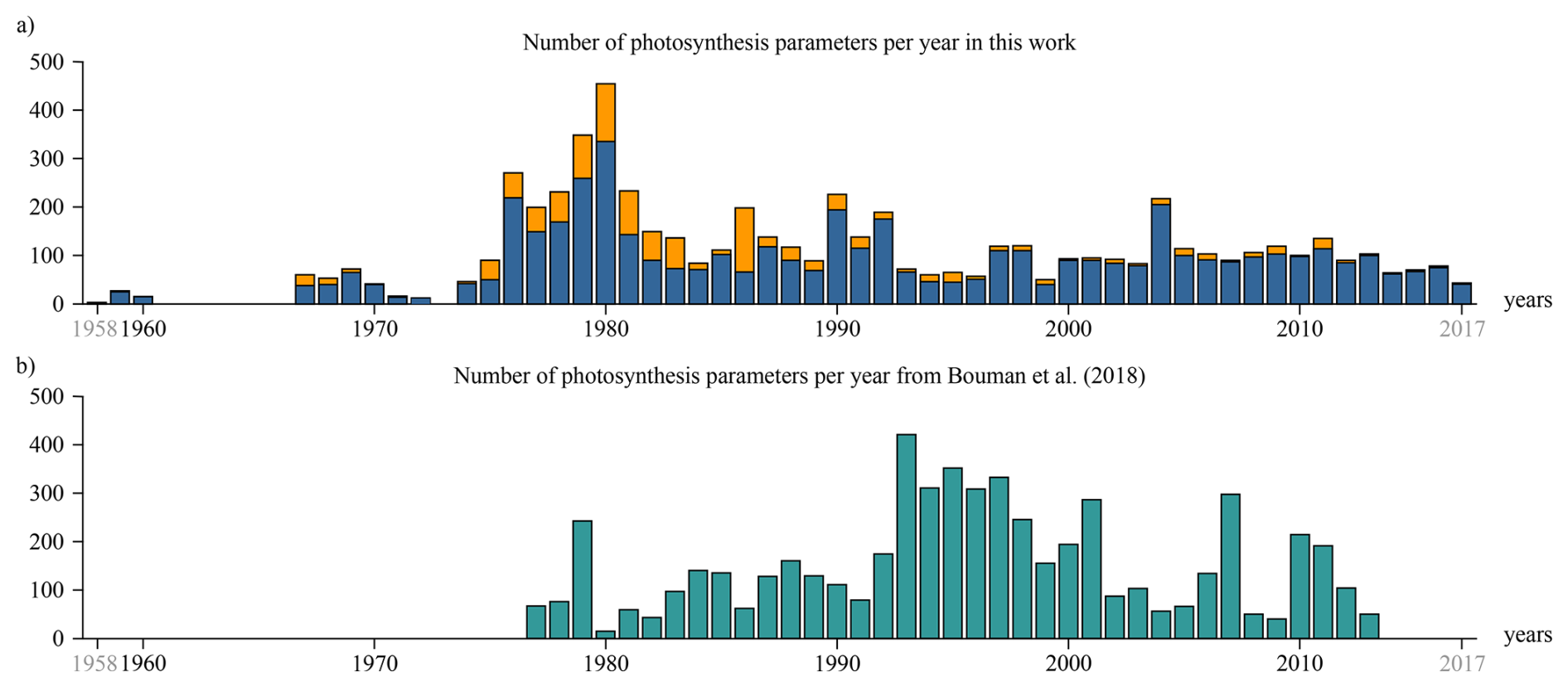
Figure 7 Time series of the global number of publicly available photosynthesis parameters. (a) Parameter values estimated from in situ production profiles under natural light conditions estimated in this work. In blue is the number of successfully estimated photosynthesis parameters, whereas in orange is the number of available production profiles (same as in Fig. 4d). (b) Parameter values estimated from in vitro experiments under controlled light conditions, published by Bouman et al. (2018), given in green.

One of the approaches to the assignment of parameters has been on the basis of ecological provinces, following the pioneering work of Longhurst et al. (1995). To implement, large amounts of field data were, and still are, required (Platt et al., 2008). These data typically include chlorophyll a, primary production, surface irradiance and the attenuation coefficient. Ideally, photosynthesis irradiance experiments are performed in as many locations and seasons as possible, and archived (Platt et al., 2017). Having photosynthesis parameters at our disposal then enables coupling of the in situ data to the remotely sensed data via various algorithmic approaches (Platt et al., 2008; Picart et al., 2014). This then makes possible the inverse, which is the assignment of photosynthesis parameters to a given region of the ocean (Platt and Sathyendranath, 1999; Devred et al., 2007).

Photosynthesis irradiance experiments have been carried out numerous times yielding parameters in various oceans and seas, with the most recent published global archive of photosynthesis parameters by Bouman et al. (2018) containing 5711 parameter values globally. Most of the Bouman et al. (2018) data are from the North Atlantic and the Arctic, with pockets of data in the Southern Ocean, Indian Ocean and in the South Atlantic, with scarcely any data in the Pacific ocean (Fig. 3), such that the global ocean is spatially undersampled with respect to photosynthesis parameters.

The photosynthesis parameters estimated from the Mattei and Scardi (2021a) dataset complement the direct estimates with respect to location (Fig. 3), filling gaps in many parts of the world ocean. The dataset contains 6084 measured production profiles from the global oceans. It is comprised of already published and freely available data, as well as some data which were less well known. By using the inverse model (Kovač et al., 2016b, a) we were able to estimate 3776 photosynthesis parameters pairs from this dataset and thereby we have created a new dataset containing photosynthesis parameters from the North Pacific Ocean, the Eastern Equatorial Pacific Ocean, close to both the east and west coasts of North America, the Indian Ocean and the northern high latitudes (Fig. 3). A large swath of the Eastern Pacific Ocean in the equatorial region is also covered. In comparison to the Bouman et al. (2018) dataset, also shown in Fig. 3, the new dataset complements and increases the spatial coverage of photosynthesis parameters in the global ocean. In both the Bouman et al. (2018) and the new dataset, there are also scattered pockets of data from various other regions of the ocean.

The two datasets are however not directly comparable given the differences in the experimental methods used to estimate primary production. The incubations in photosynthesis-irradiance experiments are typically shorter and on the order of hours, whereas the incubations in photosynthesis-depth experiments are typically longer and on the daily scale (Platt et al., 2017). Apart from the duration, the two experiments are distinct with respect to irradiance conditions: being controlled in photosynthesis-irradiance experiments, and being natural in photosynthesis-depth experiments. The estimate of the assimilation number is less affected by the quality of light (Kovač et al., 2016a), therefore the comparison of the assimilation number between the Bouman et al. (2018) dataset and this dataset is straightforward. Given the initial slope is estimated from low levels of irradiance in both experiments, and the spectral structure of irradiance changing with depth in the ocean, implies the initial slope estimated from production profiles is not directly comparable to the initial slope estimated from photosynthesis-irradiance experiments, since the spectral structure of irradiance might not be the same. Therefore, despite the parameters extracted by both methods being mathematically equivalent, given both are derived using the same mathematical model of primary production, care must be exercised with respect to the initial slope comparisons between the two methods.

From the temporal standpoint these datasets are not by any means homogenous in the number of parameters per year (Fig. 7). The number per year is low, both for the new dataset developed here, and for the Bouman et al. (2018) dataset. The Bouman et al. (2018) dataset begins in 1977 and ends in 2013, whereas the new one starts is 1960 and ends in 2017. Construction of a joint time series using both datasets would not be a trivial problem, because of the disparities in time and location. Nevertheless, construction of local time series of photosynthesis parameters would be plausible, given there are time series stations at which photosynthesis parameters have been estimated from in situ production profiles. For example, at the Hawaii Ocean Time Series and the Bermuda Atlantic Time Series, photosynthesis parameters have been estimated by Kovač et al. (2016b, 2018), respectively. Some of those data are also contained in the Mattei and Scardi (2021a) dataset. Primary production measurements are ongoing at those stations, though the latest values are not, naturally, included in the Mattei and Scardi (2021a) dataset. Measurements at Hawaii Ocean Time Series started in 1989 and at Bermuda Atlantic Time Series in 1988. In a recent work Kovač et al. (2026b) have constructed 30 years long time series at these stations. Therefore, there is a potential to construct time series of photosynthesis parameters that are at least 30 years long at these locations. The construction of such time series provides testing grounds for studying the effect of time dependent photosynthesis parameters on remote sensing algorithms and ecosystem models. This might improve the current estimates at these time series (Wu et al., 2024) and assist in future modelling efforts (Zheng et al., 2025).

Time series analysis of the photosynthesis parameters themselves would also help assess whether seasonal variability in photosynthesis parameters dominates over the interannual variability, or vice versa, and to study the rate of change of photosynthesis parameters. Information on the time scales of variability would help mold future developments in remote sensing algorithms and help in parameter assignment procedures more broadly, like in marine ecosystem models. Naturally, analysis of trends would be possible once such time series had been established. These are all potential applications of the dataset assembled here.

In this context, the importance of proper data storage and accessibility, cannot be exaggerated. This work would not have been possible without the publicly available dataset from Mattei and Scardi (2021a). From the historical standpoint, production profiles data are not distributed under a central data hub and subsequently are not easily accessible. From the standpoint of primary production models, this is unfortunate, as quality data are essential for model development and testing, arguably with a minimum standard for archiving data satisfied (Platt et al., 2017). When measuring primary production at sea, the essential variables that are typically archived are the chlorophyll a and primary production profiles. These should be complemented by archiving daily irradiance and the irradiance profile ideally, whenever available. Having such auxiliary information would allow the estimation of photosynthesis parameters, as demonstrated here. If, however, information on surface and underwater irradiance is not stored, statistical methods, such as Bayesian approaches or machine learning algorithms, could be used for estimating photosynthesis parameters. Such methods could also provide reliable uncertainty measures for photosynthesis parameters and potentially also for watercolumn production estimates. They might also be able to relax the requirement on the minimum number of vertical levels at which the production profiles have to be measured. Therefore, we recognize the application of Bayesian methods and machine learning algorithms are a potential course for future research.

A point that merits consideration is whether the parameters extracted from in situ primary production data subjected to inverse modelling techniques applied to a non-spectral model, as is done here, would be directly applicable to a spectral model of primary production. It has been demonstrated (Sathyendranath and Platt, 2007) that spectral models and non-spectral models of primary production are fundamentally different from each other in one major respect: spectral models are able to account for the spectral variability in underwater light fields, and for the covariance of spectrally-resolved light with the spectral variability in the action spectrum of photosynthesis. Here, action spectrum is the term used to describe the spectral variability in α^B. Direct measurements of action spectrum in the field are rare (but see Lewis et al., 1985; Schofield et al., 1991; Kyewalyanga et al., 1997); and so spectral models of primary production exploit the similarity in the shape of the action spectrum with that of phytoplankton absorption (Kyewalyanga et al., 1998), but allow the mean magnitude of the action spectrum to match the value of α^B measured under spectrally-neutral white light (Sathyendranath and Platt, 1989a). It is therefore important that the α^B values provided as inputs to spectral models are estimated under white light, or corrected for the spectral quality of light in the incubator. The α^B inferred from in situ primary-production profile, on the other hand, correspond to the spectral quality of the light that the phytoplankton experienced at the time of their incubations. Therefore, α^B inferred using a non-spectral model should not be used without appropriate correction to a spectral model.

Spectral quality of light becomes important when combining in situ experiments with simulated in situ incubations. In the latter, the samples are incubated on deck (rather than under water), and different filters are used to reduce the light level reaching the samples to simulate light levels reaching different depths of the water column. Often, these are neutral filters such that there is no attempt to simulate the spectral quality of light underwater. On the other hand, in some experiments, green or blue filters are used to represent better the spectral quality of light underwater. The Mattei and Scardi (2021) database contains data from in situ incubations and simulated in situ incubations. They have all been treated alike in the inverse model, and hence are subject to some unknown uncertainties associated with the spectral quality of light in the simulated in situ experiments.

In addition to this, most ocean colour models estimate primary production on a daily timescale, which aligns with both the approximate duration of phytoplankton cell division and the temporal resolution at which phytoplankton biomass can be observed using Earth-orbiting satellites (Marra, 2002). However, rate parameters derived from conventional short-term (2 to 3 h) photosynthesis irradiance incubations have been shown to exhibit diel periodicity (MacCaull and Platt, 1977; Prézelin et al., 1986; Harding et al., 1983; Bruyant et al., 2005). Such fluctuations in photosynthesis parameters are not accounted for in current primary production models, which typically assume that photosynthesis parameters remain constant throughout the day based on the assumption that diel variability is relativity minor compared to differences observed across biogeochemical provinces (Babin et al., 1996). It has also been argued that respiratory losses relative to carbon assimilation may also vary over the course of the day, which would also cause rates of carbon uptake to be dependent on the duration of the incubation (Marra, 2009). This new dataset will allow future comparisons of photosynthesis parameters derived from 24 h in situ incubations with those derived from short-term photo-physiological experiments (e.g. Bouman et al., 2018) and will allow us to assess whether the two approaches yield similar spatio-temporal patterns in photosynthetic response across a range of biogeochemical domains.

6 Data availability

The dataset of photosynthesis parameters created in this work is published in the Zenodo repository and is made publicly available (Kovač et al., 2025). It can be accessed at https://doi.org/10.5281/zenodo.17973417.

7 Code availability

The code for accessing and analysing the original Mattei and Scardi (2021a) dataset is published in the Zenodo repository and is made publicly available (Kovač et al., 2026a). It can be accessed at https://doi.org/10.5281/zenodo.22645060.

8 Conclusions

In this work we have derived a global set of photosynthesis parameters estimated from primary production profiles published by Mattei and Scardi (2021a). In the parameter estimation procedure we have used an analytically solvable model of the production profile by Kovač et al. (2016b) as the forward model (Fig. 1). For the inverse model we have used an optimization procedure with the Nelder and Mead (1965) search algorithm, constrained by the analytical solution for watercolumn production by Platt et al. (1990). We have discussed the advantages, as well as the limitations of the approach stemming from both the model and the data (Figs. 2 and 4). The overall model versus data comparison was performed on watercolumn production, as shown in Fig. 6, demonstrating good internal model reconstruction performance.

The new dataset of photosynthesis parameters that was constructed in this work is complementary to the prior dataset published by Bouman et al. (2018) and provides a comparable spatio-temporal coverage (Figs. 3 and 7). With this work the global archive of publicly available data on photosynthesis parameters has effectively doubled. A straightforward application of the new photosynthesis parameters dataset is in global primary production models, such as by Kulk et al. (2020, 2021), or in biogeochemical models, such as by Follows et al. (2007). The new dataset is publicly available at https://doi.org/10.5281/zenodo.17973417 (Kovač et al., 2025), along with metadata for referencing it to the original Mattei and Scardi (2021a) dataset.

Having the new dataset available opens the avenue for novel research directions, such as testing existing remote sensing models with the novel parameter values in regions of the ocean where non where known prior, constructing local or regional algorithms for photosynthesis parameters assignment, or constructing time series of photosynthesis parameters. Also, having demonstrated that the recovery of photosynthesis parameters from such a large global dataset is plausible, the application of other methods and models, might as well be a potential course for future research. From an operational standpoint, we conclude that creating a global hub for primary production data, be it production profiles, or photosynthesis irradiance experiments, is due.

Appendix A: Notation

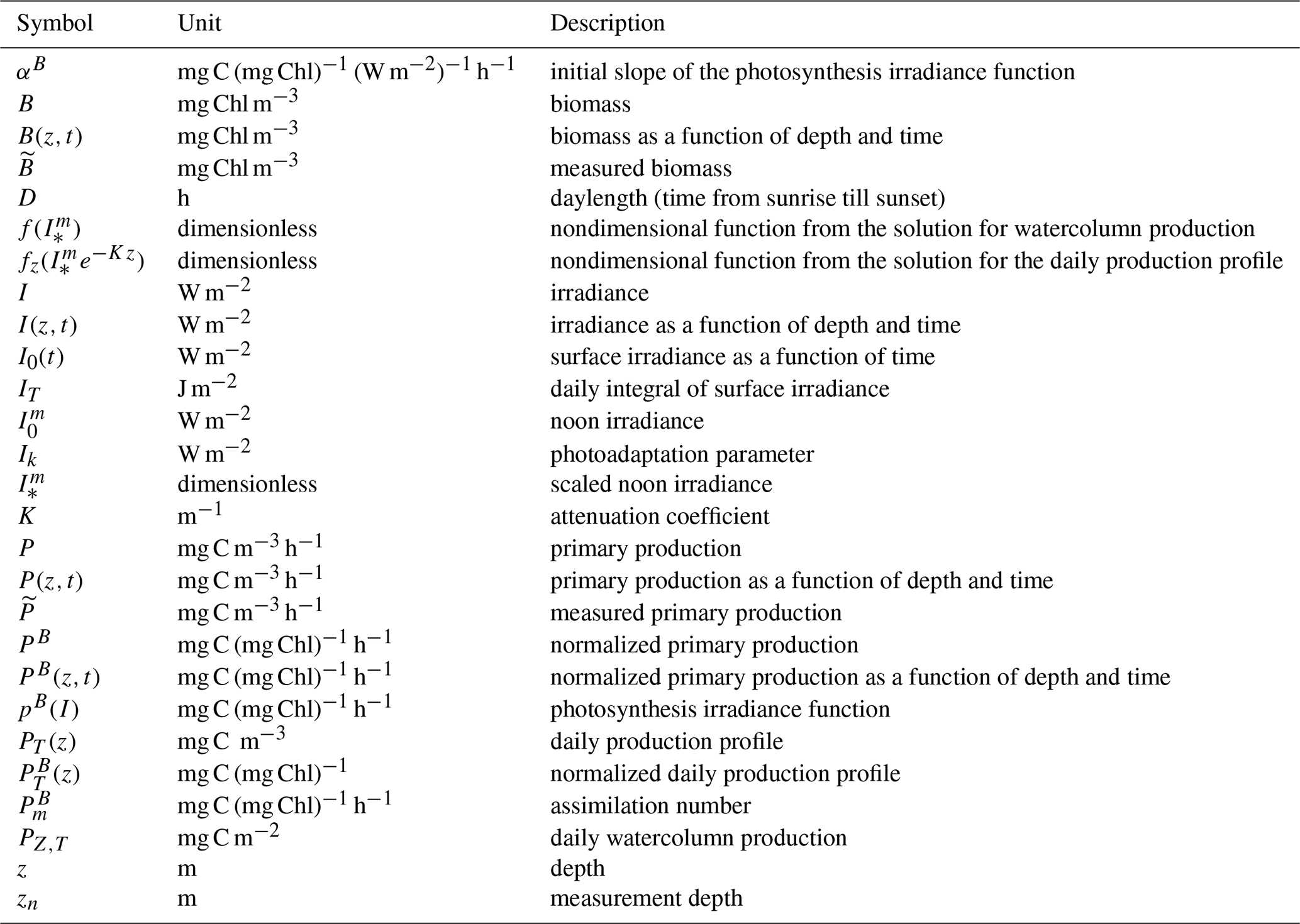
Table A1 List of mathematical symbols used in the manuscript along with their units and short descriptions.

Appendix B: Forward model

The primary production model used in this paper is based on the work of Platt et al. (1990) in which the exponential photosynthesis irradiance function from a previous paper, also by Platt et al. (1980), is used in Eq. (1):

$$\begin{array}{}\text{(B1)}& p^B\left(I\right)=P_m^B\left(\mathrm{1}-\exp \left(-{\mathit{\alpha }}^{B}I/P_m^B\right)\right).\end{array}$$

The underwater irradiance model is as stated in Eq. (4). Platt et al. (1990) have solved the watercolumn production integral (Eq. 6) exactly for the case of uniform time independent biomass $B(z,t)=B$. Their solution reads:

$$\begin{array}{}\text{(B2)}& P_{Z,T}={\displaystyle \frac{B{P}_m^{B}D}{K}}f\left(I_{*}^m\right),\end{array}$$

where the $f\left(I_{*}^m\right)$ function is given as:

$$\begin{array}{}\text{(B3)}& \begin{array}{rl}f\left(I_{*}^m{e}^{-Kz}\right)& =\sum _{n=\mathrm{1}}^{\mathrm{\infty }}{\displaystyle \frac{\mathrm{2}{\left(I_{*}^m{e}^{-Kz}\right)}^{\mathrm{2}n-\mathrm{1}}}{\mathit{\pi }\left(\mathrm{2}n-\mathrm{1}\right)\left(\mathrm{2}n-\mathrm{1}\right)\mathrm{!}}}{\displaystyle \frac{\left(\mathrm{2}n-\mathrm{2}\right)\mathrm{!}\mathrm{!}}{\left(\mathrm{2}n-\mathrm{1}\right)\mathrm{!}\mathrm{!}}}\\ & -\sum _{n=\mathrm{1}}^{\mathrm{\infty }}{\displaystyle \frac{{\left(I_{*}^m{e}^{-Kz}\right)}^{\mathrm{2}n}}{\mathrm{2}n\left(\mathrm{2}n\right)\mathrm{!}}}{\displaystyle \frac{\left(\mathrm{2}n-\mathrm{1}\right)\mathrm{!}\mathrm{!}}{\left(\mathrm{2}n\right)\mathrm{!}\mathrm{!}}}.\end{array}\end{array}$$

By rearranging expression (B2) the analytical solution for normalised watercolumn production Eq. (18) is obtained:

$$\begin{array}{}\text{(B4)}& P_{Z,T}^B={\displaystyle \frac{P_m^{B}D}{K}}f\left(I_{*}^m\right).\end{array}$$

Based on the solution (B4), in a paper by Kovač et al. (2016b), the analytical solution of the integral for the normalised daily production profile (5) was solved. It reads:

$$\begin{array}{}\text{(B5)}& P_T^B\left(z\right)=P_m^{B}D{f}_z\left(I_{*}^m{e}^{-Kz}\right),\end{array}$$

where now the $f_z\left(I_{*}^m{e}^{-Kz}\right)$ function is given as:

$$\begin{array}{}\text{(B6)}& \begin{array}{rl}{f}_z\left(I_{*}^m{e}^{-Kz}\right)& =\sum _{n=\mathrm{1}}^{\mathrm{\infty }}{\displaystyle \frac{\mathrm{2}{\left(I_{*}^m{e}^{-Kz}\right)}^{\mathrm{2}n-\mathrm{1}}}{\mathit{\pi }\left(\mathrm{2}n-\mathrm{1}\right)\mathrm{!}}}{\displaystyle \frac{\left(\mathrm{2}n-\mathrm{2}\right)\mathrm{!}\mathrm{!}}{\left(\mathrm{2}n-\mathrm{1}\right)\mathrm{!}\mathrm{!}}}\\ & -\sum _{n=\mathrm{1}}^{\mathrm{\infty }}{\displaystyle \frac{{\left(I_{*}^m{e}^{-Kz}\right)}^{\mathrm{2}n}}{\left(\mathrm{2}n\right)\mathrm{!}}}{\displaystyle \frac{\left(\mathrm{2}n-\mathrm{1}\right)\mathrm{!}\mathrm{!}}{\left(\mathrm{2}n\right)\mathrm{!}\mathrm{!}}}.\end{array}\end{array}$$

The two functions, Eqs. (B3) and (B6), are related by:

$$\begin{array}{}\text{(B7)}& f_z\left(I_{*}^m{e}^{-Kz}\right)=-{\displaystyle \frac{\mathrm{1}}{K}}{\displaystyle \frac{\mathrm{d}}{\mathrm{d}z}}f\left(I_{*}^m{e}^{-Kz}\right).\end{array}$$

From Eq. (B5) the daily production profile is simply calculated by multiplication with biomass:

$$\begin{array}{}\text{(B8)}& P_T=B\left(z\right)P_m^{B}D{f}_z\left(I_{*}^m{e}^{-Kz}\right),\end{array}$$

where B(z) is prescribed. The normalised daily production profile (B5) and the normalised daily watercolumn production are then used in the optimal function of the inverse model (11) to estimate photosynthesis parameters from a measured normalised daily production profile.

Appendix C: Inverse model

For an individual survey, we have at disposal the following set of measurements: noon irradiance ${\stackrel{\mathrm{̃}}{I}}_{\mathrm{0}}^m$, attenuation coefficient $\stackrel{\mathrm{̃}}{K}$, daylength $\stackrel{\mathrm{̃}}{D}$, production profile ${\stackrel{\mathrm{̃}}{P}}_T\left(z_n\right)$ and biomass profile $\stackrel{\mathrm{̃}}{B}\left(z_n\right)$, where $n=\mathrm{1},\mathrm{2},\mathrm{\dots },N$. By calculating the measured normalised production profile as:

$$\begin{array}{}\text{(C1)}& {\stackrel{\mathrm{̃}}{P}}_T^B\left(z_n\right)={\stackrel{\mathrm{̃}}{P}}_T\left(z_n\right)/\stackrel{\mathrm{̃}}{B}\left(z_n\right)\end{array}$$

we formulate the error of the forward model as:

$$\begin{array}{}\text{(C2)}& \begin{array}{rl}\mathcal{P}\left({\mathit{\alpha }}^B,P_m^B\right)& =\sum _{n=\mathrm{1}}^N\left(P_m^B\stackrel{\mathrm{̃}}{D}{f}_z\left({\mathit{\alpha }}^B{\stackrel{\mathrm{̃}}{I}}_{\mathrm{0}}^m{e}^{-\stackrel{\mathrm{̃}}{K}{z}_n}/P_m^B\right)\right.\\ & {\left.-{\stackrel{\mathrm{̃}}{P}}_T^B\left(z_n\right)\right)}^{\mathrm{2}}+\left({\displaystyle \frac{P_m^B\stackrel{\mathrm{̃}}{D}}{\stackrel{\mathrm{̃}}{K}}}f\right({\mathit{\alpha }}^B{\stackrel{\mathrm{̃}}{I}}_{\mathrm{0}}^m/P_m^B)\\ & -\sum _{n=\mathrm{1}}^N{\stackrel{\mathrm{̃}}{P}}_T^B\left(z_z\right)\mathrm{\Delta }{z}_n{)}^{\mathrm{2}},\end{array}\end{array}$$

This function is then used as the optimal function in the inverse model. The first sum in the optimal function goes over the measurement depths and compares the model prediction $P_T^B\left(z_n\mid {\mathit{\alpha }}^B,P_m^B\right)$ with the measured value at that depth ${\stackrel{\mathrm{̃}}{P}}_T^B\left(z_n\right)$ (green dots on the right in Fig. 1). The second term compares the model prediction of normalised watercolumn production $P_m^B\stackrel{\mathrm{̃}}{D}f({\mathit{\alpha }}^B{\stackrel{\mathrm{̃}}{I}}_{\mathrm{0}}^m/P_m^B)/\stackrel{\mathrm{̃}}{K}$ with the measured normalised daily watercolumn production ${\sum }_{n=\mathrm{1}}^N{\stackrel{\mathrm{̃}}{P}}_T^B\left(z_z\right)\mathrm{\Delta }{z}_n$ (blue surface on the right in Fig. 1). The photosynthesis parameter values at the minimum of $\mathcal{P}\left({\mathit{\alpha }}^B,P_m^B\right)$ are taken as the optimal values and are labelled as: ${\widehat{\mathit{\alpha }}}^B$ and ${\widehat{P}}_m^B$.

In the implementation stage of the inverse model we have opted to use the Nelder-Mead optimization algorithm (Nelder and Mead, 1965), a direct search algorith already tested on this type of problems by Kovač et al. (2016b, a). To reduce the search in the parameter space we have set the constraints on the photosynthesis parameters to be positive, namely α^B>0 and $P_m^B>\mathrm{0}$, given that by definition the parameters are positive. Also, the two analytical expressions used in the optimal function (C2), one for the normalised daily production profile and the other for the normalied daily watercolumn produciton, are both infinite sums. This implies that at implementation these sums have to be truncated and we have opted to truncate both at 50 elements in the sum.

Appendix D: Statistical measures

Here we list the statistical measures used for estimating model performance based on the work of Li et al. (2022). Variable $\stackrel{\mathrm{̃}}{x}$ stands for measurement and x for model. The notation 〈x〉 is used to denote the mean of x. Coefficient of determination is calculated as:

$$\begin{array}{}\text{(D1)}& R^{\mathrm{2}}=\mathrm{1}-{\displaystyle \frac{\sum _{i=\mathrm{1}}^N\left[\log \right(x_i)-\log ({\stackrel{\mathrm{̃}}{x}}_i){]}^{\mathrm{2}}}{\sum _{i=\mathrm{1}}^N\left[\log \right({\stackrel{\mathrm{̃}}{x}}_i)-\langle \log (\stackrel{\mathrm{̃}}{x}\left)\right]\rangle {]}^{\mathrm{2}}}},\end{array}$$

which is expressed as percentages. The root mean square difference is calculated as:

$$\begin{array}{}\text{(D2)}& \mathrm{RMSD}=\sqrt{{\displaystyle \frac{\mathrm{1}}{N}}\sum _{i=\mathrm{1}}^N\left[\log \right(x_i)-\log ({\stackrel{\mathrm{̃}}{x}}_i){]}^{\mathrm{2}}}.\end{array}$$

The unbiased absolute percentage difference is calculated as:

$$\begin{array}{}\text{(D3)}& \mathrm{UAPD}={\displaystyle \frac{\mathrm{1}}{N}}\sum _{i=\mathrm{1}}^N\left|{\displaystyle \frac{\mathrm{2}(x_i-{\stackrel{\mathrm{̃}}{x}}_i)}{x_i+{\stackrel{\mathrm{̃}}{x}}_i}}\right|,\end{array}$$

also expressed as percentages. The logarithmic bias is calculated as:

$$\begin{array}{}\text{(D4)}& \mathrm{LB}=\left({\mathrm{10}}^Z-\mathrm{1}\right),\end{array}$$

again expressed as percentages and where Z is given by:

$$\begin{array}{}\text{(D5)}& Z={\displaystyle \frac{\mathrm{1}}{N}}\sum _{i=\mathrm{1}}^N\left[\log \right(x_i)-\log ({\stackrel{\mathrm{̃}}{x}}_i\left)\right].\end{array}$$

More details on these measures can be found in Li et al. (2022).